On Self-Distilling Graph Neural Network

Abstract

Recently, the teacher-student knowledge distillation framework has demonstrated its potential in training Graph Neural Networks (GNNs). However, due to the difficulty of training over-parameterized GNN models, one may not easily obtain a satisfactory teacher model for distillation. Furthermore, the inefficient training process of teacher-student knowledge distillation also impedes its applications in GNN models. In this paper, we propose the first teacher-free knowledge distillation method for GNNs, termed GNN Self-Distillation (GNN-SD), that serves as a drop-in replacement of the standard training process. The method is built upon the proposed neighborhood discrepancy rate (NDR), which quantifies the non-smoothness of the embedded graph in an efficient way. Based on this metric, we propose the adaptive discrepancy retaining (ADR) regularizer to empower the transferability of knowledge that maintains high neighborhood discrepancy across GNN layers. We also summarize a generic GNN-SD framework that could be exploited to induce other distillation strategies. Experiments further prove the effectiveness and generalization of our approach, as it brings: 1) state-of-the-art GNN distillation performance with less training cost, 2) consistent and considerable performance enhancement for various popular backbones.

1 Introduction

Knowledge Distillation (KD) has demonstrated its effectiveness in boosting compact neural networks. Yet, most of the KD researches focus on Convolutional Neural Networks (CNNs) with regular data as input instances, while little attention has been devoted to Graph Neural Networks (GNNs) that are capable of processing irregular data. A significant discrepancy is that GNNs involve the topological information into the updating of feature embeddings across network layers, which is not taken into account in the existing KD schemes, restricting their potential extensions to GNNs.

A recent work, termed LSP Yang et al. (2020), proposed to combine KD with GNNs by transferring the local structure, which is modeled as the distribution of the similarity of connected node pairs, from a pre-trained teacher GNN to a light-weight student GNN. However, there exists a major concern on the selection of qualified teacher GNN models. On the one hand, it’s likely to cause performance degradation once improper teacher networks are selected Tian et al. (2019). On the another hand, the performance of GNNs is not always indicated by their model capacity due to the issues of over-smoothing Li et al. (2018) and over-fitting Rong et al. (2019), which have caused obstacles to train over-parameterized and powerful GNNs. As a result, every time encountering a new learning task, one may spend substantial efforts in searching for a qualified GNN architecture to work as a teacher model, and thus the generalization ability of this method remains a challenge. Another barrier of the adopted conventional teacher-student framework is the inefficiency in the training process. Such distillation pipeline usually requires two steps: first, pre-training a relatively heavy model, and second, transferring the forward predictions (or transformed features) of the teacher model to the student model. With the assistance of the teacher model, the training cost would tremendously increase more than twice than an ordinary training procedure.

In this work, we resort to cope with these issues via the self-distillation techniques (or termed teacher-free distillation), which perform knowledge extraction and transfer between layers of a single network without the assistance from auxiliary models Zhang et al. (2019); Hou et al. (2019). Our work provides the first dedicated self-distillation approach designed for generic GNNs, named GNN-SD. The core ingredient of GNN-SD is motivated by the mentioned challenge of over-smoothing, which occurs when GNNs go deeper and lead the node features to lose their discriminative power. Intuitively, one may avoid such dissatisfied cases by pushing node embeddings in deep layers to be distinguishable from their neighbors, which is exactly the property possessed by shallow GNN layers.

To this end, we first present the Neighborhood Discrepancy Rate (NDR) to serve as an approximate metric in quantifying the non-smoothness of the embedded graph at each GNN layer. Under such knowledge refined by NDR, we propose to perform knowledge self-distillation by an adaptive discrepancy retaining (ADR) regularizer. The ADR regularizer adaptively selects the target knowledge contained in shallow layers as the supervision signal and retains it to deeper layers. Furthermore, we summarize a generic GNN-SD framework that could be exploited to derive other distillation strategies. As an instance, we extend GNN-SD to involve another knowledge source of compact graph embedding for better matching the requirements of graph classification tasks. In a nutshell, our main contributions are:

• We present GNN-SD, to our knowledge, the first generic framework designed for distilling the graph neural networks with no assistance from extra teacher models. It serves as a drop-in replacement of the standard training process to improve the training dynamics.

• We introduce a simple yet efficient metric of NDR to refine the knowledge from each GNN layer. Based on it, the ADR regularizer is proposed to empower the adaptive knowledge transfer inside a single GNN model.

• We validate the effectiveness and generalization ability of our GNN-SD by conducting experiments on multiple popular GNN models, yielding the state-of-the-art distillation result and consistent performance improvement against baselines.

2 Related Work

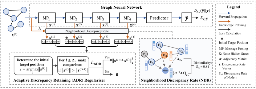
Figure 1: The schemata of the distillation strategy of adaptive discrepancy retaining. A four-layer GNN is adopted for the illustration.

Graph Neural Network

Recently, Graph Neural Networks (GNNs), which propose to perform message passing across nodes in the graph and updating their representation, has achieved great success on various tasks with irregular data, such as node classification, protein property prediction to name a few. Working as a crucial tool for graph representation learning, however, these models encounter the challenge of over-smoothing. It says that the representations of the nodes in GNNs would converge to a stationary point and become indistinguishable from each other when the number of layers in GNNs increases. This phenomenon limits the depth of the GNNs and thus hinders their representation power.

One solution to alleviate this problem is to design network architectures that can better memorize and utilize the initial node features. Representative papers includes GCN Kipf and Welling (2016), JKNet Xu et al. (2018b) DeeperGCN Li et al. (2020), GCNII Chen et al. (2020b), etc. On the other hand, methods like DropEdge Rong et al. (2019) and AdaEdge Chen et al. (2020a) have proposed solutions from the view of conducting data augmentation.

In this paper, we design a distillation approach tailored for GNNs, which also provides a feasible solution to this problem. Somewhat related, Chen et al. Chen et al. (2020a) proposed a regularizer to the training loss, which simply forces the nodes in the last GNN layer to obtain a large distance between remote nodes and their neighboring nodes. However, it can only obtain a slight performance improvement.

Teacher-Student Knowledge Distillation

Knowledge distillation Hinton et al. (2015), aims at transferring the knowledge hidden in the target network (i.e. teacher model) into the online network (i.e. student model) that is typically light-weight, so that the student achieves better performance compared with the one trained in an ordinary way. Generally, there exist two technical routes for KD. The first one is closely related to label smoothing Yuan et al. (2020), which utilizes the output distribution of the teacher model to serve as a smooth label for training the student. Another line of research is termed as feature distillation Romero et al. (2014); Zagoruyko and Komodakis (2016); Kim et al. (2018), which exploits the semantic information contained in the intermediate representations. As summarized in Heo et al. (2019), with different concerning knowledge to distill, these methods can be distinguished by the formulation of feature transformation and knowledge matching loss function.

Recently,  Yang et al. Yang et al. (2020) studied the teacher-student distillation methods in training GNNs. They extract the knowledge of local graph structure based on the similarity of connected node pairs from the teacher model and student model, then perform distillation by forcing the student model to match such knowledge. However, the performance improvement resulted from the teacher-student distillation framework does not come with a free price, as discussed in Section 1.

Self-Distillation

For addressing the issues of the teacher-student framework, a new research area termed teacher-free distillation, or self-distillation, attracts a surge of attention recently. Throughout this work, we refer this notion to the KD techniques that perform knowledge refining and transfer between network layers inside a single model. In this way, the distillation learning could be conducted with a single forward propagation in each training iteration. BYOT Zhang et al. (2019) proposed the first self-distillation method. They consider that the teacher and student are composed in the same networks since the deeper part of the networks can extract more semantic information than the shallow one. Naturally, they manage to distill feature representations as well as the smooth label from deeper layers into the shallow layers. Similarly, Hou et al. Hou et al. (2019) proposed to distill the attention feature maps from the deep layers to shallow ones for lane detection. However, these methods focus on the application of CNNs, neglecting the usage of graph topology information, and thus restricting their potential extension to GNNs.

3 GNN Self-Distillation

A straightforward solution to perform self-distillation for training GNNs is to supervise the hidden states of shallow layers by the ones of deep layers as the target, as the scheme proposed in BYOT Zhang et al. (2019). However, we empirically find that such a strategy leads to performance degradation. It’s on the one hand attributed to the neglection of the graph topological information. On the other hand, it’s too burdensome for shallow GNN layers to match their outputs to such unrefined knowledge and eventually leads to over-regularizing. Furthermore, such a simple solution requires fixed representation dimensionalities across network layers, which limits its applications to generic GNN models. In the following sections, we first introduce the key ingredient of our GNN Self-Distillation (GNN-SD). Then we summarize a unified GNN-SD framework that is well extendable to other distillation variants.

Notation

Throughout this work, a graph is represented as $\mathcal{G}=\{\mathcal{V},\mathcal{E},\mathbf{A}\}$, where $\mathcal{V}$ is vertex set that has $N$ nodes with $d$-dimension features of $\mathbf{X}\in\mathbb{R}^{N\times d}$, edge set $\mathcal{E}$ of size $M$ is encoded with edge features of $\mathbf{E}$, and $\mathbf{A}\in\mathbb{R}^{N\times N}$ is the adjacency matrix. The node degree matrix is given by $\mathbf{D}=\mathrm{diag}(\mathbf{A}\mathbf{1}_{N})$. Node hidden states of $l$-th GNN layer is denoted as $\mathbf{X}^{(l)}$, and the initial hidden states $\mathbf{X}^{(0)}$ is usually set as the node intrinsic features $\mathbf{X}$. Given a node $v$, its connected-neighbors are denoted as $\mathcal{N}_{v}$. For a matrix $\mathbf{X}$, $\mathbf{X}_{i\cdot}$ denotes its $i$-th row and $\mathbf{X}_{\cdot j}$ denotes its $j$-th column.

3.1 Adaptive Discrepancy Retaining

Since the well-known over-smoothing issue of GNNs occurs when the input graph data flows into deep layers, an inspired insight is that we can utilize the property of non-smoothness in shallow GNN layers, and distill such knowledge into deep ones. In this way, the model is self-guided to retain non-smoothness from the initial embedded graph to the final embedded output. The remained questions are: how to refine the desired knowledge from the fine-grained node embeddings? and what is a proper knowledge transfer strategy?

Neighborhood Discrepancy Rate

To answer the first question, we introduce the module of Neighborhood Discrepancy Rate (NDR), which is used to quantify the non-smoothness of each GNN layer.

It’s proved that nodes in a graph component converge to the same stationary point while iteratively updating the message passing process of GNNs, and hence the hidden states of connected-nodes become indistinguishable Li et al. (2018). It implies that, given a node $v$ in the graph,

$$\sum\nolimits_{c\in\mathcal{N}_{v}}\|\mathbf{X}_{v\cdot}^{(l)}-\mathbf{X}_{c\cdot}^{(l)}\|_{p}<\epsilon,\text{if}\;l\to\infty,\forall\epsilon>0.$$ (1)

As a result, it leads to the issue of over-smoothing and further hurts the accuracy of node classification. Centering around this conclusion, it is a natural choice to use the pair-wise metric (and the resulting distance matrix) to define the local non-smoothness of the embedded graph. However, such fine-grained knowledge might still cause over-regularization for GNNs trained under teacher-free distillation. By introducing the following proposition (details deferred to Appendix A), one can easily derive from formula (1) that, $\|\mathbf{X}_{v\cdot}^{(l)}-(\mathbf{D}^{-1}\mathbf{A}\mathbf{X})_{v\cdot}^{(l)}\|_{p}<\epsilon$ as layer $l$ goes to infinity.

Proposition 1. Suppose $d_{1}(\mathbf{X},\mathcal{G})$ calculates the $L_{p}$-norm of the difference of each central node and their aggregated neighbors in the graph $\mathcal{G}$, and the pair-wise distance metric $d_{2}(\mathbf{X},\mathcal{G})$, on the other hand, computes the difference at the level of node pairs. Then, the inequality holds: $d_{2}(\mathbf{X},\mathcal{G})\geq d_{1}(\mathbf{X},\mathcal{G})$.
We leverage this property to refine the knowledge from a higher level. Specifically, given a central node $v$ in layer $l$, we first obtain the aggregation of its adjacent nodes to work as the virtual node that indicates its overall neighborhood, $\mathbf{N}_{v}^{(l)}=(\mathbf{D}^{-1}\mathbf{A}\mathbf{X}^{(l)})_{v\cdot}$. For excluding the effect of embeddings’ magnitude, we use the cosine similarity between the embeddings of central node $\mathbf{X}^{(l)}_{v\cdot}$ and virtual node $\mathbf{N}^{(l)}_{v}$ to calculate their affinity, and transform it into a distance metric,

$$S_{v}^{(l)}=1-\frac{{\mathbf{X}^{(l)}_{v\cdot}}(\mathbf{A}\mathbf{X}^{(l)})_{v\cdot}^{\text{T}}}{||\mathbf{X}^{(l)}_{v\cdot}||_{2}\cdot||(\mathbf{A}\mathbf{X}^{(l)})_{v\cdot}||_{2}},v=1,...,N,$$ (2)

Note that it’s not needed to perform the inverse matrix multiplication of node degrees due to the normalization conducted by cosine similarity metric. The defined $S_{v}^{(l)}$ of all nodes compose the neighborhood discrepancy rate of layer $l$:

$$\mathbf{s}^{(l)}=(S_{1}^{(l)},...,S_{N}^{(l)}).$$ (3)

Compared with the pair-wise metric, the NDR extracts neighbor-wise non-smoothness, which is easier to transfer and prevents over-regularizing by self-distillation. Moreover, it can be easily implemented with two consecutive matrix multiplication operations, enjoying a significant computational advantage. The NDR also possesses better flexibility to model local non-smoothness of the graph, since pair-wise metrics can not be naturally applied together with layer-wise sampling techniques Chen et al. (2018); Huang et al. (2018).

Specially, for the task of node classification, there is another reasonable formulation of the virtual neighboring node. That is, taking node labels into account, $\mathbf{N}_{v}^{(l)}=(\mathbf{D}^{-1}\mathbf{A}^{{}^{\prime}}\mathbf{X}^{(l)})_{v\cdot}$, where $\mathbf{A}^{{}^{\prime}}=\mathbf{A}\odot\mathbf{Y}$ denotes the masked adjacency, $\mathbf{Y}\in\mathbb{R}^{N\times N}$ the binary matrix with entries $\mathbf{Y}_{i,j}$ equal to 1 if node $i$ and $j$ are adjacent and belong to different categories, and $\odot$ the element-wise multiplication operator. Then, the NDR would not count the discrepancy of nodes that are supposed to share high similarity. For unity and simplicity, we still use the former definition throughout this work.

Strategy for Retaining Neighborhood Discrepancy

Previous self-distillation methods usually treat the deep representations as the target supervision signals, since they are considered to contain more semantic information. However, we found that such a strategy is not optimal, sometimes even detrimental for training GNNs (refer to Appendix D for details). The rationale behind our design of distilling neighborhood discrepancy is to retain the non-smoothness, which is extracted as the knowledge by NDR, from shallow GNN layers to the deep ones. In details, we design the following guidelines (refer to Appendix F for more analysis) for the self-distillation learning, which formulate our adaptive discrepancy retaining (ADR) regularizer:

• The noise in shallow network layers might cause the calculated NDR of the first few embedded graphs to be inaccurate, thus the initial supervision target is adaptively determined by the magnitude of the calculated NDR.

• For facilitating the distillation learning, the knowledge transfer should be progressive. Hence, the ADR loss is computed by matching the NDR of deep layer (online layer) to the target one of its previous layer (target layer).

• Explicit and adaptive teacher selection is performed, i.e the ADR regularizes the GNN only when the magnitude of NDR of the target layer is larger than the online layer.

• Considering that the nodes in regions of different connected densities have different rates of becoming over-smoothing Li et al. (2018), the matching loss can be weighted by the normalized node degrees to emphasize such a difference.

As a result, the final ADR regularizer is defined as:

$$\mathcal{L}_{\mathrm{N}}=\sum_{l=l^{\star},...,L-1}\mathbbm{1}(\|\mathbf{s}^{(l)}\|\textgreater\|\mathbf{s}^{(l+1)}\|)d^{2}(\mathbf{s}^{(l+1)},\mathbf{s}^{(l)}),$$ (4)

where the indicator function $\mathbbm{1}(\cdot)$ performs the teacher selection, $l^{\star}=\mathrm{argmax}_{k}\{\|\mathbf{s}^{(k)}\||k\in\{1,...,L-1\}\}$ determine the position of initial supervision target, and $d^{2}(\mathbf{s}^{(l+1)},\mathbf{s}^{(l)})=\|\mathbf{D}(\mathbf{s}^{(l+1)}-\mathrm{SG}(\mathbf{s}^{(l)}))^{\text{T}}\|_{2}^{2}$ is the degree-weighted mean squared error function that calculates the knowledge matching loss. Here $\mathrm{SG}(\cdot)$ denotes the Stop Gradient operation, meaning that the gradient of the target NDR tensor is detached in the implementation, for serving as a supervision signal. The approach is depicted in Figure 1.

In addition, we analytically demonstrate that the proposed notion of discrepancy retaining can be comprehended from the perspective of information theory. This is analogous to the concept in Ahn et al. (2019). Specifically, the retaining of neighborhood discrepancy rate encourages the online layer to share high mutual information with the target layer, as illustrated in the following proposition ($I$ stands for mutual information and $H$ denotes the entropy, details are deferred to Appendix B).

Proposition 2. The optimization of the ADR loss increase the lower bound of the mutual information between the target NDR and the online one. That is, the inequality holds: $I(\mathbf{s}^{(l)},\mathbf{s}^{{(l+1)}})\geq H(\mathbf{s}^{(l)})-\mathbbm{E}_{\mathbf{s}^{(l)},\mathbf{s}^{(l+1)}}[\|\mathbf{D}(\mathbf{s}^{(l+1)}-\mathbf{s}^{(l)})^{\text{T}}\|_{2}^{2}]$.

3.2 Generic GNN-SD Framework

Generally, by refining and transferring compact and informative knowledge between layers, self-distillation on GNNs can be summarized as the learning of the additional mapping,

$$\mathcal{M}_{\mathrm{SD}}^{g,L}:\mathcal{T}_{s}(\mathcal{C}_{s}(\mathcal{G},P_{s}))\to\mathcal{T}_{t}(\mathcal{C}_{t}(\mathcal{G},P_{t})),$$ (5)

where $P\in\{1,...,L\}$ is the layer position to extract knowledge from the network, $\mathcal{C}$ denotes the granularity (or coarseness) of the embedded graph, $\mathcal{T}$ represents the specific transformation applied to the chosen embeddings, and the subscripts of $s$ and $t$ denote the identity of student (to simulate) and teacher (to transfer), respectively.

Naturally, the combinations of different granularities and transformation functions lead to various distilled knowledge. As an instance, we show here to involve another knowledge source of the full-graph embedding, and provide further discussions in Appendix E for completeness.

Considering the scenario of graph classification, where GNNs might focus more on obtaining meaningful embedding of the entire graph than individual nodes, the full-graph embedding could be the well-suited knowledge, since it provides a global view of the embedded graph (while the NDR captures the local property),

$$\mathcal{C(\mathcal{G},P)}:=\mathbf{G}^{(P)}=\mathrm{Readout}_{v\in\mathcal{G}}(\mathbf{X}^{(P)}_{v\cdot}),$$ (6)

where $\mathrm{Readout}$ is a permutation invariant operator that aggregates embedded nodes to a single embedding vector. In contrast to the fine-grained node features, the coarse-grained graph embedding is sufficiently compact so as we can simply use the identity function to preserve the transferred knowledge. Hence the target mapping is:

$$\mathcal{M}_{\mathrm{graph}}^{g,L}:\mathbf{\mathds{1}}(\mathbf{G}^{(l+1)})\to\mathbf{\mathds{1}}(\mathbf{G}^{(l)}).$$ (7)

It can be learned by optimizing the graph-level distilling loss:

$$L_{\mathrm{G}}=\sum\nolimits_{l=1,...,L-1}||\mathbf{G}^{(l+1)}-\mathrm{SG}(\mathbf{G}^{(l)})||_{2}^{2}.$$ (8)

In this way, GNN-SD extends the utilization of mixed knowledge sources over different granularities of the embedded graph.

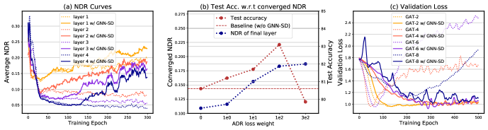
Figure 2: (a) Comparison of NDR between training w/ (solid line) and w/o (dotted line) imposing ADR regularizer. Smaller value means suffering from more over-smoothing. (b) The correlation between test accuracy and converged NDR of the final layer, controlled by the loss weights of ADR regularizer. (c) Comparison of validation loss curves. GAT-$n$ denotes GAT model with $n$ hidden layers.

Overall Loss

The total loss function is formulated as:

$$\mathcal{L}_{\mathrm{T}}=\mathrm{CE}(g(\mathbf{X}^{(L)}),y)+\alpha\mathcal{L}_{\mathrm{L}}+\beta\mathcal{L}_{\mathrm{N}}+\gamma\mathcal{L}_{\mathrm{G}}.$$ (9)

The first term calculates the basic cross entropy loss between the final predicted distribution and the ground-truth label $y$. The second term, borrowing from Zhang et al. (2019), regularizes the intermediate logits generated by intermediate layers to mimic the final predicted distribution for accelerating the training and improving the capacity of shallow layers. The remaining terms are defined in Eq.(4) and Eq.(8). $\alpha$, $\beta$, and $\gamma$ are the hyper-parameters that balance the supervision of the distilling objectives and target label.

4 Experiments

4.1 Exploring Analysis of Discrepancy Retaining

We first conduct exploring analysis to investigate how the ADR regularizer helps improve the training dynamics of GNNs. Hyper-parameters of $\alpha$ and $\gamma$ are fixed to $0$.

In Figure  2(a), we show the comparison of NDR curves of each layer in a $4$-layer GraphSage Hamilton et al. (2017). In line with the expectations, the neighborhood discrepancy in a GNN model drops when the layer grows, and the final layer (in dark blue, dotted line) approaches a close-to-zero value of NDR, which indicates that the output node embeddings become indistinguishable with their neighbors. Conversely, the GNN trained with GNN-SD preserves higher discrepancy over shallow to deep layers, and even reveals an increasing tendency as the training progresses. It might imply that the GNN gradually learns to pull the connected-node embeddings away if they’re not of the same class, for obtaining more generalized representations. This observation indicates ADR’s effect on alleviating the over-smoothing issue. We also provide related examples in Appendix F that motivate the development of ADR regularizer.

In Figure  2(b), we study the correlation of model performance and the converged NDR: as the ADR loss weight increases in a reasonable range (e.g. from $1e0$ to $1e2$), the NDR increases and the performance gain improves (from $0.6\%$ to $2.5\%$). The shown positive correlation between test accuracy and NDR verifies the rationality of the NDR metric and the distillation strategy as well. Notably, there also exists a trade-off in determining the optimal loss weight. If an over-estimated weight ($1e3$) was assigned, the knowledge transfer task would become too burdensome for the GNN model to learn the main classification task and hurt the performance.

Figure  2(c) depicts the validation loss on GAT Veličković et al. (2018) backbones with different depths. The validation loss curves are dramatically pulled down after applying GNN-SD. It explains that ADR regularizer also helps GNNs relieve the issue of over-fitting, which is known as another tough obstacle in training deep GNNs.

Table 1: Performance comparison with other distillation methods. The second column indicates the knowledge source, $\mathbf{X}$ is node features, $\mathbf{A}$ is the adjacency matrix, $T(\cdot)$ denotes the teacher model.

Method	Knowledge Source	F1 Score	Time
Teacher ($T$)	/	$97.6$	0.85s
Baseline	/	$95.7$	0.62s
AT	$T(\mathbf{X})$	$95.4$	1.75s
FitNet	$T(\mathbf{X})$	$95.6$	1.99s
LSP	$T(\mathbf{X})$,$T(\mathbf{A})$	$96.1$	1.90s
Baseline	/	$95.61_{\pm 0.20}$	0.62s
AT	$\mathbf{X}$	$95.88_{\pm 0.25}$	0.73s
FitNet	$\mathbf{X}$	$95.60_{\pm 0.17}$	0.95s
BYOT	$\mathbf{X}$	$95.81_{\pm 0.56}$	0.80s
GNN-SD	$\mathbf{X}$,$\mathbf{A}$	$\textbf{96.20}_{\pm 0.03}$	0.87s

4.2 Comparison with KD Methods

We compare our method with other distillation methods, including AT Zagoruyko and Komodakis (2016), FitNet Romero et al. (2014), BYOT Zhang et al. (2019) and LSP Yang et al. (2020). We follow Yang et al. (2020) to perform the comparisons on the baseline of a 5-layer GAT on the PPI dataset Zitnik and Leskovec (2017). For evaluating AT and FitNet in a teacher-free KD scheme, we follow their papers to perform transformations on node embeddings to get the attention maps and intermediate features, respectively. We also evaluate BYOT to see the effect of intermediate logits. The experiments are conducted for 4 runs, and those under teacher-student framework are cited from Yang et al. (2020). For our method, the hyper-parameters of $\alpha$ and $\beta$ are both set to $0.01$ and $\gamma$ is $0$. Training time (per epoch) of each model is measured on a NVIDIA 2080 Ti GPU. Results are summarized in Table 1. More details are deferred to Appendix G. Clearly, GNN-SD obtains significant performance promotion against other self-distillation methods by involving the topological information into the refined knowledge. GNN-SD also achieves a better performance gain (0.59) on the baseline compared with LSP (0.4), even when our method does not require the assistance from an extra teacher model. In this way, the training cost is greatly saved (40$\%$ training time increase against baseline for GNN-SD v.s. 190$\%$ increase for LSP). Besides, it avoids the process of selecting qualified teachers, bringing much better usability.

Table 2: Node classification on varying-depths models.

Dataset	Model	Layers
		2	4	8	16
Cora	GAT	83.2	80.1	76.9	74.8
	GAT w/ GNN-SD	83.7	81.2	80.1	77.6
	GraphSage	81.3	80.3	78.8	77.2
	GraphSage w/ GNN-SD	81.7	81.5	79.8	78.2
Citeseer	GAT	72.5	70.5	65.1	64.5
	GAT w/ GNN-SD	72.6	71.5	68.3	66.2
	GraphSage	72.3	70.7	61.7	59.2
	GraphSage w/ GNN-SD	72.7	71.0	64.5	61.8
Pubmed	GAT	79.2	78.5	76.6	75.6
	GAT w/ GNN-SD	79.5	79.4	78.5	76.6
	GraphSage	78.8	77.9	73.8	77.2
	GraphSage w/ GNN-SD	79.2	79.4	77.6	78.2

4.3 Overall Comparison Results

Node Classification

Table 2 summarizes the results of GNNs with various depths on the citation classification datasets, including Cora, Citeseer and PubMed Sen et al. (2008). We follow the setting of semi-supervised learning, using the fixed 20 nodes per class for training. The hyper-parameters of $\gamma$ is fixed to $0$ for node classification, and we determine $\alpha$ and $\beta$ via a simple grid search. Details are provided in Appendix H. It’s observed that GNN-SD consistently improves the test accuracy for all cases. Generally, GNN-SD yields larger improvement for deeper architecture, as it gains $0.5\%$ average improvement for a two-layer GAT on Cora while achieving $3.2\%$ increase for the 8-layer one.

Graph Classification

Table 3 summarizes the results of various popular GNNs on the graph kernel classification datasets, including ENZYMES, DD, and PROTEINS in TU dataset Kersting et al. (2016). Since there exist no default splittings, each experiment is conducted by 10-fold cross validation with the splits ratio at 8:1:1 for training, validating and testing. We choose five widely-used GNN models, including GCN, GAT, GraphSage, GIN Xu et al. (2018a) and GatedGCN Bresson and Laurent (2017), to work as the evaluation baselines. Hyper-parameter settings are deferred to Appendix I. Again, one can observe that GNN-SD achieves consistent and considerable performance enhancement against all the baselines. On classification of PROTEINS, for example, even the next to last model trained with GNN-SD (GraphSage, $76.71\%$) outperforms the best model (GAT, $76.36\%$) trained in the ordinary way. The results further validate the generalization ability of our self-distilling strategy.

Table 3: Graph classification on various GNN backbones. The top 2 models on each dataset are bolded.

Dataset	Model	Baseline	w/ GNN-SD	Gain
ENZYMES	GCN	$64.00_{\pm 5.63}$	$66.66_{\pm 3.94}$	$(+2.66)$
	GAT	$65.33_{\pm 5.90}$	$68.00_{\pm 2.66}$	$(+2.66)$
	GraphSage	$68.33_{\pm 6.41}$	$\mathbf{70.00}_{\pm 5.05}$	$(+1.66)$
	GIN	$66.00_{\pm 7.19}$	$\textbf{69.33}_{\pm 4.02}$	$(+3.33)$
	GatedGCN	$65.33_{\pm 4.52}$	$67.33_{\pm 1.33}$	$(+2.00)$
DD	GCN	$77.83_{\pm 1.02}$	$\mathbf{78.67}_{\pm 1.68}$	$(+0.84)$
	GAT	$76.65_{\pm 2.51}$	$77.50_{\pm 2.50}$	$(+0.85)$
	GraphSage	$76.14_{\pm 1.66}$	$77.49_{\pm 1.89}$	$(+1.35)$
	GIN	$73.00_{\pm 3.90}$	$74.77_{\pm 3.50}$	$(+1.77)$
	GatedGCN	$77.83_{\pm 1.67}$	$\textbf{78.20}_{\pm{1.98}}$	$(+0.37)$
PROTEINS	GCN	$75.55_{\pm 2.91}$	$76.81_{\pm 3.19}$	$(+1.26)$
	GAT	$76.36_{\pm 2.77}$	$\mathbf{77.53}_{\pm 3.38}$	$(+1.17)$
	GraphSage	$75.55_{\pm 4.02}$	$76.71_{\pm 3.81}$	$(+1.15)$
	GIN	$64.86_{\pm 3.03}$	$70.06_{\pm 4.89}$	$(+5.20)$
	GatedGCN	$76.36_{\pm 3.94}$	$\textbf{76.90}_{\pm 3.68}$	$(+0.54)$

Table 4: Compatibility study. Experiments are conducted under the full-supervised scheme, following DropEdge’s implementation.

Models	Layers
	8	16	32	50
Baseline	78.1±0.9	79.1±1.1	79.3±0.8	78.4±1.1
w/ DropEdge	79.4±0.7	79.3±0.9	79.4±1.2	78.7±0.9
w/ GNN-SD	79.1±0.8	79.9±0.5	79.7±1.1	79.2±0.8
w/ Both	80.1±0.6	79.6±0.8	80.2±0.8	79.6±0.5

Compatibility Evaluation

There exist other methods that aim at facilitating the training of GNNs. One influential work is DropEdge Rong et al. (2019), which randomly samples graph edges to introduce data augmentation. We conduct experiments on JKNet Xu et al. (2018b) and Citeseer dataset to evaluate the compatibility of these orthogonal training schemes. The edge sampling ratio in DropEdge is searched at the range of $\{0.1,...,0.9\}$, with results demonstrated in Table 4. It reads that while both GNN-SD and DropEdge are capable of improving the training, GNN-SD might perform better on deep backbones. Notably, employing them concurrently is likely to deliver further promising enhancement.

Table 5: Ablation study of different knowledge sources.

	GNN-B	GNN-L	GNN-N	GNN-G	GNN-M
$\mathcal{L}_{\mathrm{L}}$		$\surd$			$\surd$	$\surd$
$\mathcal{L}_{\mathrm{N}}$			$\surd$		$\surd$	$\surd$
$\mathcal{L}_{\mathrm{G}}$				$\surd$		$\surd$
Cora	$80.12$	$\pagecolor{lightgray}{79.83}$	$80.83$	/	81.16	/
Citeseer	$70.53$	$71.16$	$71.43$	/	71.52	/
Pubmed	$78.52$	$\pagecolor{lightgray}{78.53}$	79.44	/	$79.26$	/
ENZYMES	$66.00$	$66.66$	$67.66$	$67.66$	$66.66$	69.33
DD	$73.00$	$73.76$	74.77	$73.51$	$73.76$	$74.14$

4.4 Ablation Studies

We perform an ablation study to evaluate the knowledge sources and identify the effectiveness of our core technique, as shown in Table 5. We select GAT as the evaluation backbone for node classification and GIN for graph classification. We name the baseline as ‘GNN-B’, and model solely distilled by intermediate logits Zhang et al. (2019), neighborhood discrepancy, and compact graph embedding as ‘GNN-L’, ‘GNN-N’, ‘GNN-G’, respectively. The models distilled by mixed knowledge are represented as ‘GNN-M’. One observation from the results is that simply adopting the intermediate logits seems to fail in bring consistent improvement (highlighted in gray), while it may cooperate well with other sources since it promotes the updating of shallow features (highlighted in blue). In contrast, the discrepancy retaining plays the most important role in distillation training. For graph classifications, the involvement of compact graph embedding also contributes well while jointly works with the others.

5 Conclusion

We have presented an efficient yet generic GNN Self-Distillation (GNN-SD) framework tailored for boosting GNN performance. Experiments verify that it achieves state-of-the-art distillation performance. Meanwhile, serving as a drop-in replacement of the standard training process, it yields consistent and considerable enhancement on various GNN models.

Appendix

Appendix A Proof of Proposition 1

For simplicity, here we use the $L_{p}$-norm to measure the vector difference. Pair-wise distance metric $d_{2}(\mathbf{X},\mathcal{G})$ calculates the total sum of all node pairs dissimilarity, as follows:

$$d_{2}(\mathbf{X},\mathcal{G}) =\frac{1}{|\mathcal{E}|}\sum_{v\in\mathcal{V}}\sum_{c\in\mathcal{N}(v)}||\mathbf{X}_{v\cdot}-\mathbf{X}_{c\cdot}||_{p}$$

$$\geq\frac{1}{|\mathcal{E}|}\sum_{v\in\mathcal{V}}||\sum_{c\in\mathcal{N}(v)}(\mathbf{X}_{v\cdot}-\mathbf{X}_{c\cdot})||_{p}$$

$$=\frac{1}{|\mathcal{E}|}\sum_{v\in\mathcal{V}}||\mathbf{D}_{v,v}(\mathbf{X}_{v\cdot}-\frac{(\mathbf{A}\mathbf{X})_{v\cdot}}{\mathbf{D}_{v,v}})||_{p}$$

$$\geq\frac{1}{|\mathcal{E}|}\sum_{v\in\mathcal{V}}||\mathbf{X}_{v\cdot}-(\mathbf{D}^{-1}\mathbf{A}\mathbf{X})_{v\cdot}||_{p}$$ (10)

The RHS of the last inequality computes the sum of dissimilarity between nodes and their 1-hop aggregated neighbors, formulating the neighbor-wise distance $d_{1}(\mathbf{X},\mathcal{G})$. The proof is concluded.

Appendix B Proof of Proposition 2

The mutual information between the NDR of consecutive layers is defined as:

$$I(\mathbf{s}^{(l)},\mathbf{s}^{(l+1)}) =H(\mathbf{s}^{(l)})-H(\mathbf{s}^{(l)}|\mathbf{s}^{(l+1)})$$

$$=-\mathbbm{E}_{\mathbf{s}^{(l)}}[\mathrm{log}p(\mathbf{s}^{(l)})]+\mathbbm{E}_{\mathbf{s}^{(l)},\mathbf{s}^{(l+1)}}[\mathrm{log}p(\mathbf{s}^{(l)}|\mathbf{s}^{(l+1)})],$$ (11)

since the true conditional probability is not intractable, we resort to the help with the variational distribution of $q(\mathbf{s}^{(l)}|\mathbf{s}^{(l+1)})$ that approximates $p(\mathbf{s}^{(l)}|\mathbf{s}^{(l+1)})$, and study the lower bound of the mutual information. Continuing from formula (B),

$$I(\mathbf{s}^{(l)},\mathbf{s}^{(l+1)}) =H(\mathbf{s}^{(l)})+\mathbbm{E}_{\mathbf{s}^{(l)},\mathbf{s}^{(l+1)}}[\mathrm{log}p(\mathbf{s}^{(l)}|\mathbf{s}^{(l+1)})]$$

$$=H(\mathbf{s}^{(l)})+\mathbbm{E}_{\mathbf{s}^{(l)},\mathbf{s}^{(l+1)}}[\mathrm{log}q(\mathbf{s}^{(l)}|\mathbf{s}^{(l+1)})]+\mathbbm{E}_{\mathbf{s}^{(l)}}[\mathrm{D_{KL}}(p(\mathbf{s}^{(l)}|\mathbf{s}^{(l+1)})||q(\mathbf{s}^{(l)}|\mathbf{s}^{(l+1)}))]$$

$$\geq H(\mathbf{s}^{(l)})+\mathbbm{E}_{\mathbf{s}^{(l)},\mathbf{s}^{(l+1)}}[\mathrm{log}q(\mathbf{s}^{(l)}|\mathbf{s}^{(l+1)})],$$ (12)

here we can adopt the Gaussian distribution with heteroscedastic expectation $\mu=\mathbf{s}^{(l+1)}$ and variance $\sigma={\mathbf{1}_{N}}^{\text{T}}\mathbf{D}$ as the variational distribution. And it’s assumed with the property that NDR of nodes are conditionally independent given the ones of subsequent layer. That is, $q(\mathbf{s}^{(l)}|\mathbf{s}^{(l+1)})=\prod_{v}q(S_{v}^{(l)})|S_{v}^{(l+1)})=\prod_{v}\frac{1}{\mathbf{D}_{v,v}\sqrt{2\pi}}\mathrm{exp}(-\frac{(S_{v}^{(l)}-S_{v}^{(l+1)})^{2}}{2\mathbf{D}_{v,v}^{2}})$. Then, the logarithm of variational distribution is expressed as:

$$\mathrm{log}q(\mathbf{s}^{(l)}|\mathbf{s}^{(l+1)}) =\sum_{v=1,...,N}\mathrm{log}q(S^{(l)}_{v}|S_{v}^{(l+1)})$$

$$=\sum_{v=1,...,N}-\mathrm{log}\frac{1}{\mathbf{D}_{v,v}}-\frac{(S^{(l)}_{v}-S^{(l+1)}_{v})^{2}}{1/\mathbf{D}_{v,v}}+\text{constant}.$$ (13)

Since the node degree $\mathbf{D}_{v,v}$ is fixed and $-\mathrm{log}\frac{1}{\mathbf{D}_{v,v}}$ is greater than zero, then combining equation (B) and (B) leads to:

$$I(\mathbf{s}^{(l)},\mathbf{s}^{{(l+1)}})\geq H(\mathbf{s}^{(l)})-\mathbbm{E}_{\mathbf{s}^{(l)},\mathbf{s}^{(l+1)}}[\|\mathbf{D}(\mathbf{s}^{(l+1)}-\mathbf{s}^{(l)})^{\text{T}}\|_{2}^{2}].$$ (14)

The proof is concluded.

Appendix C Experimental Environments

Most experiments conducted in this paper are run on a NVIDIA 2080 Ti GPU with 11 GB memory, except for very-deep GNNs, which are conducted on a NVIDIA Tesla P40 with 24GB memory. Experiments are mainly implemented by PyTorch of version 1.3.1 and DGL Wang and et al. [2019] of version 0.4.2.

Appendix D Comparison on Two Supervision Schemes of Retaining NDR

Table 6 compares the results of two supervision schemes: Transferring the NDR of shallow layers to deep ones and the reverse strategy. Since the rationale of our design is to retain high neighborhood discrepancy from shallow layers to deep layers, the common strategy for CNN models that transfers knowledge from deep layers to shallow layers is not the desired scheme for conducting GNN-SD. One can see that performing neighborhood discrepancy retaining by serving the NDR of deep embeddings as supervision targets is not optimal, sometimes even detrimental for GNN models. These results verify our conjecture.

Table 6: Comparison of two schemes of NDR transferring, in accuracy gain ($\%$). Performing neighborhood discrepancy retaining by serving the NDR of embeddings in the shallow layer as supervision signals is denoted as ‘shallow2deep’, and the other one is ‘deep2shallow’. A 3-layer GAT is selected as the baseline.

GAT	Cora	Citeseer	Pubmed
shallow2deep	+0.66	+0.73	+0.80
deep2shallow	-0.52	-0.22	+0.17

Appendix E The Generic GNN Self-Distillation Framework

Recall the summarized self-distillation objective,

$$\mathcal{M}_{\mathrm{SD}}^{g,L}:\mathcal{T}_{s}(\mathcal{C}_{s}(\mathcal{G},P_{s}))\to\mathcal{T}_{t}(\mathcal{C}_{t}(\mathcal{G},P_{t})),$$

the various combination of granularity settings and transformation functions leave wide space for further exploration. Generally, the choices of granularities of a graph $\mathcal{C}(\mathcal{G},P)$ constitute the set of $\{\mathbf{X}^{(P)},\mathbf{E}^{(P)},\mathbf{SG}^{(P)},\mathbf{G}^{(P)}\}$, which is made up of: 1) fine-grained embeddings at node and edge levels, denoted as $\mathbf{X}$ and $\mathbf{E}$, 2) coarse-grained embeddings at full-graph and sub-graph levels, denoted as $\mathbf{G}\in{{\mathbb{R}}}^{1\times d}$ and $\mathbf{SG}\in\mathbb{R}^{s\times d}$ of:

$$\mathbf{G}=\mathrm{Readout}_{v\in\mathcal{G}}(\mathbf{X}_{v\cdot})$$

$$\mathbf{SG}_{i\cdot}=\mathrm{Readout}_{v\in\mathcal{SG}_{i}}(\mathbf{X}_{v\cdot}),\quad i=1,2,...,s$$ (15)

where $s$ represents the number of partitioned sub-graphs, $\mathcal{SG}_{i}=\{\mathcal{V}_{i},\mathcal{E}_{i},\mathbf{A}_{i}\}$ is the $i$th sub-graph that consists of the corresponding vertex and edge subsets and adjacency. The straightforward approach to generate sub-graph is to perform random sampling schemes on the original graph. It remains an interesting problem that how to sample representative nodes in cooperate with the distillation target.

In practice, the chosen granularity depends on the specific scenario and goal that wishes to obtain by self-distillation. The transformation should comprise between the properties of ‘easy to learn’ and ‘avoid information missing’. In the manuscript, we have adopted the fine-grained node embeddings $\mathbf{X}$ and coarse-grained full-graph embedding $\mathbf{G}$ to perform a mixed knowledge self-distillation for training GNNs. The core technique of discrepancy retaining performs distillation in a progressive manner, results in the objective instance of:

$$\mathcal{M}_{\mathrm{node}}^{g,L}:\mathrm{NDR}(\mathbf{X}^{(l+1)})\to\mathrm{NDR}(\mathbf{X}^{(l)}),$$ (16)

where $\mathrm{NDR}(\cdot)$ is formulated by Eq.(2) and Eq.(3). We have further involved knowledge sources of the full-graph embedding in our GNN-SD framework, as illustrated in formula (7).

In fact, the training objective of formula (7) can be naturally extended to sub-graph level by replacing $\mathbf{G}$ by $\mathbf{SG}$. For applying the GNN-SD to edge features $\mathbf{E}$, a simple two-step solution is to firstly transform the node-adjacency matrix $\mathbf{A}$ into edge-adjacency matrix of $\mathbf{A}^{e}$, where each element is:

$$[\mathbf{A}^{e}]_{i,j}=\begin{cases}1&i\cap j\neq\emptyset,\;\text{edge $i$, $j$ share a same node}\\ 0&\text{otherwise}\end{cases}$$ (17)

and then extend the NDR to edge-level by replacing Eq.(2) with:

$$S_{i}^{e}=1-\frac{{\mathbf{E}_{i\cdot}}^{\top}{(\mathbf{A}^{e}\mathbf{E})}_{i\cdot}}{||\mathbf{E}_{i\cdot}||_{2}\cdot||(\mathbf{A}^{e}\mathbf{E})_{i\cdot}||_{2}},i=1,...,M.$$ (18)

It’s worthy noting that the transformation $\mathcal{T}$ can not only be manually designed but learned during the training process. A linear layer or $\mathrm{MLP}$ is able to facilitate the student layers to match the target knowledge, which leads formula (16), for example, to the following variant:

$$\mathcal{M}_{\mathrm{node}}^{g,L}:\mathrm{NDR}(f(\mathbf{X}^{(P_{s})}))\to\mathrm{NDR}(\mathbf{X}^{(P_{t})}),$$ (19)

where $f$ denotes the learnable function. We empirically find that this technique is typically useful for distillation on large-scale datasets and very-deep GNNs.

Appendix F Additional NDR Curves Exemplars

Figure 3 shows the NDR Curves of the 8-layer GCN and GraphSage on OGB-arxiv dataset. It’s observed that the initial embedded graph (in light yellow) has low NDR value (in average), which might be caused by the fact that the first GNN layer takes much more noise. In GCN, the embedded graph of the second layer (in orange) possesses the highest NDR across the training stage, while in GraphSage it appears alternation that the third layers (in tomato) become more discriminated in the late training stage. The above observations motivate us to adaptively select the initial target supervision signal.

Furthermore, we find that the consecutive intermediate layers could show minor overlap in the average NDR, and it doesn’t make sense to perform knowledge retaining for the case that the target layer show lower neighborhood discrepancy than the online layer. Thus we introduce explicit teacher selection in the ADR regularizer.

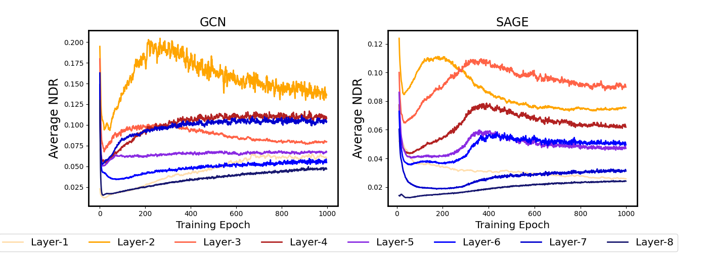
Figure 3: NDR curves of the two 8-layers GNNs. Smaller value meanssuffering from more over-smoothing.

We provide a comparison study to show the effect of the adaptive distillation strategy, with results in Table 7. Here, the ‘naive matching’ denotes that the distillation loss is defined as $\mathcal{L}_{\mathrm{N}}=\sum_{l=1,...,L-1}d^{2}(\mathbf{s}^{(l+1)},\mathbf{s}^{(l)})$.

Table 7: The effect of the adaptive self-distillation.

OGB-arxiv	GCN	GraphSage	Cora	GCN	GraphSage
baseline	71.84±0.18	71.12±0.38	baseline	80.67±1.14	79.28±1.91
naive matching	72.08±0.20	71.62±0.32	naive matching	82.70±0.97	79.97±1.81
adaptive matching	72.34±0.32	71.88±0.23	adaptive matching	82.92±0.89	80.31±2.35

Appendix G Details of the Comparison with Other Distillation Methods

For processing the PPI dataset, where possesss relative large scale graphs, we adopt a learnable linear layer in the knowledge transformation function to facilitate knowledge transfer between layers, and thus the resulting distillation object is the same as formula (19).

Table 8 describe the hyper-parameters of the teacher model used in those teacher-student KD methods, and the ones of baseline student model. One can notice that the teacher model is set in an fatter architecture with fewer layers compared with the student, which is not as usual in the conventional settings on CNNs. This confirms our concern about the difficulty of selecting a qualified teacher GNN model. In Table 9, we provide the detailed four runs results of the re-implemented baseline backbone used in LSP and our GNN-SD method.

Table 8: Settings of the baseline backbone used on the PPI dataset for comparing with LSP.

Model	Layers	Attention heads	Hidden features	#Params
Teacher ($T$)	3	4,4,6	256,256,121	3.64M
Baseline	5	2,2,2,2,2	68,68,68,68,121	0.16M

Table 9: Performance comparison on the PPI dataset. The second column records the experiment results reported in the paper of LSP. In the other columns, we report the overall running results of 4 runs of our experiments.

Method	F1 Score
	Report	our runnning results
		Avg.	(1st	2nd	3rd	4th )
Baseline	$95.7^{\star}$	95.6	(95.64	95.83	95.27	95.69)
GNN-SD	/	96.2	(96.14	96.24	96.22	96.20)

Appendix H Hyper-parameter Settings of the Node Classification Experiments, Table 2

Table 10 gives the description of the meaning of the hyper-parameters. We search the hyper-parameters for GNNs under varying depths to obtain the fair and strong baselines. For generating intermediate logits, we leverage a sharing-weights 2-layer $\mathrm{MLP}$ to take intermediate graph embeddings as input. Loss weight of $\alpha$ is searched at the range of $\{0,0.001,0.01,0.1,1\}$, $\beta$ in $\{0.001,0.01,0.1,1,10,100\}$. Table 11 summarizes the detail settings.

Table 10: Hyper-parameter Description

Hyperparameter	Description
lr	learning rate
weight-decay	L2 regularization weight
dropout	dropout rate
#layer	number of hidden layers
#hidden	hidden dimensionality
#head	number of attention heads
#epoch	number of training epochs
$\alpha$, $\beta$, $\gamma$	loss weight in Eq.(9)

Table 11: The hyper-parameters of each backbones under varying depths for citation datasets classificatoin, and the selected optimal loss weights.

Dataset	Backbone	Layers	Model Hyperparameters	Loss Hyperparameters
Cora	GAT	2	lr=1e-2, weight-decay=1e-3, dropout=0.5, #hidden=64, #head=4, #epoch=300	$\alpha=0.01,\beta=0.001$
		4	lr=1e-2, weight-decay=1e-2, dropout=0.5, #hidden=128, #head=4, #epoch=300	$\alpha=1.0,\beta=1.0$
		8	lr=1e-2, weight-decay=1e-3, dropout=0.1, #hidden=64, #head=4, #epoch=300	$\alpha=1.0,\beta=1.0$
		16	lr=1e-2, weight-decay=1e-2, dropout=0.1, #hidden=16, #head=4, #epoch=300	$\alpha=0.001,\beta=0.1$
	GraphSage	2	lr=1e-2, weight-decay=1e-3, dropout=0.5, #hidden=64, #epoch=300	$\alpha=0,\beta=0.001$
		4	lr=1e-2, weight-decay=1e-3, dropout=0.5, #hidden=64, #head=4, #epoch=300	$\alpha=0.01,\beta=1.0$
		8	lr=1e-2, weight-decay=1e-3, dropout=0.1, #hidden=64, #epoch=300	$\alpha=1.0,\beta=0.001$
		16	lr=1e-3, weight-decay=1e-2, dropout=0.1, #hidden=128, #epoch=300	$\alpha=0.001,\beta=0.001$
Citeseer	GAT	2	lr=1e-2, weight-decay=1e-3, dropout=0.8, #hidden=128, #head=4, #epoch=300	$\alpha=0,\beta=0.001$
		4	lr=1e-2, weight-decay=1e-2, dropout=0.6, #hidden=256, #head=4, #epoch=300	$\alpha=1.0,\beta=0.01$
		8	lr=1e-2, weight-decay=1e-2, dropout=0.1, #hidden=128, #head=4, #epoch=300	$\alpha=0.1,\beta=0.01$
		16	lr=1e-2, weight-decay=1e-4, dropout=0.1, #hidden=16, #head=4, #epoch=300	$\alpha=0,\beta=1.0$
	GraphSage	2	lr=1e-2, weight-decay=1e-2, dropout=0.6, #hidden=128, #epoch=300	$\alpha=0,\beta=10.0$
		4	lr=1e-2, weight-decay=1e-3, dropout=0.2, #hidden=128, #head=4, #epoch=300	$\alpha=0,\beta=0.01$
		8	lr=1e-2, weight-decay=1e-3, dropout=0.1, #hidden=128, #epoch=300	$\alpha=0.001,\beta=0.1$
		16	lr=1e-3, weight-decay=1e-2, dropout=0.1, #hidden=128, #epoch=300	$\alpha=0.01,\beta=0.001$
Pubmed	GAT	2	lr=1e-2, weight-decay=1e-3, dropout=0.1, #hidden=64, #head=4, #epoch=300	$\alpha=0.1,\beta=0.1$
		4	lr=1e-2, weight-decay=1e-2, dropout=0.1, #hidden=128, #head=4, #head=4, #epoch=300	$\alpha=0,\beta=10.0$
		8	lr=1e-2, weight-decay=1e-2, dropout=0.1, #hidden=64, #head=4, #epoch=300	$\alpha=0,\beta=0.1$
		16	lr=1e-3, weight-decay=1e-3, dropout=0.1, #hidden=128, #head=4, #epoch=300	$\alpha=1.0,\beta=100.0$
	GraphSage	2	lr=1e-2, weight-decay=1e-3, dropout=0.2, #hidden=128, #epoch=300	$\alpha=0.01,\beta=0.01$
		4	lr=1e-2, weight-decay=1e-2, dropout=0.1, #hidden=64, #head=4, #epoch=300	$\alpha=0.1,\beta=0.001$
		8	lr=1e-3, weight-decay=1e-2, dropout=0.3, #hidden=64, #epoch=300	$\alpha=0.1,\beta=10.0$
		16	lr=1e-3, weight-decay=1e-2, dropout=0.1, #hidden=128, #epoch=300	$\alpha=1.0,\beta=100.0$

Appendix I Hyper-parameter Settings of the Graph Classification Experiments, Table 3

We adopt the Adam optimizer Kingma and Ba [2014] for model training in this paper. For conducting 10-fold cross validation on graph kernel datasets, the random seed is fixed for reproducing the results. The hyper-parameters (e.g. the number of hidden dimensions) of the baseline models are set for matching the budget that each model contains around $100$k parameters. The $\mathrm{Readout}$ operator in Eq.(6) is set as the same as the one used in the baseline GNN backbone. For generating intermediate logits, we leverage a sharing-weights 2-layer $\mathrm{MLP}$ to take intermediate graph embeddings as input. Specially, GIN model which has already contained intermediate prediction layers to generate residual probability scores for the final output distribution, no extra $\mathrm{MLP}$ is introduced. For the choice of the hyper-parameters of $\alpha$, $\beta$ and $\gamma$ in Eq.(9), we carried out a simple grid search at the range of $\alpha\in\{0,0.1,1\}$, $\beta\in\{0,0.1,1\}$, $\gamma\in\{0,0.01,0.1,1\}$ for each controlled experiments. Then, the detailed hyper-parameters are summarized in Table 12.

Table 12: The hyper-parameters of each backbones on graph kernel datasets for matching the baseline budgets, and the selected optimal loss weights.

Dataset	Backbone	Model Hyperparameters	Loss Hyperparameters
ENZYMES	GCN	lr=7e-4, weight-decay=0, dropout=0, #layer=4, #hidden=128, #epoch=1000	$\alpha=0,\beta=0.1,\gamma=0$
	GAT	lr=1e-3, weight-decay=0, dropout=0, #layer=4, #hidden=16, #head=8, #epoch=1000	$\alpha=1,\beta=0.1,\gamma=0$
	GraphSage	lr=7e-4, weight-decay=0, dropout=0, #layer=4, #hidden=96, #epoch=1000	$\alpha=0,\beta=1,\gamma=0$
	GIN	lr=7e-3, weight-decay=0, dropout=0, #layer=4, #hidden=96, #epoch=1000	$\alpha=0.1,\beta=1,\gamma=1$
	GatedGCN	lr=7e-4, weight-decay=0, dropout=0, #layer=4, #hidden=64, #epoch=1000	$\alpha=1,\beta=0.1,\gamma=0$
DD	GCN	lr=1e-5, weight-decay=0, dropout=0, #layer=4, #hidden=128, #epoch=1000	$\alpha=0,\beta=0,\gamma=0.01$
	GAT	lr=5e-5, weight-decay=0, dropout=0, #layer=4, #hidden=16, #head=8, #epoch=1000	$\alpha=0,\beta=0.1,\gamma=0$
	GraphSage	lr=1e-5, weight-decay=0, dropout=0, #layer=4, #hidden=96, #epoch=1000	$\alpha=1,\beta=0,\gamma=0$
	GIN	lr=1e-3, weight-decay=0, dropout=0, #layer=4, #hidden=96, #epoch=1000	$\alpha=0,\beta=1,\gamma=0$
	GatedGCN	lr=1e-5, weight-decay=0, dropout=0, #layer=4, #hidden=64, #epoch=1000	$\alpha=0,\beta=0.1,\gamma=0.01$
PROTEINS	GCN	lr=7e-4, weight-decay=0, dropout=0, #layer=4, #hidden=128, #epoch=1000	$\alpha=0,\beta=1,\gamma=0$
	GAT	lr=1e-3, weight-decay=0, dropout=0, #layer=4, #hidden=16, #head=8, #epoch=1000	$\alpha=0,\beta=0,\gamma=0.01$
	GraphSage	lr=7e-5, weight-decay=0, dropout=0, #layer=4, #hidden=96, #epoch=1000	$\alpha=0,\beta=1,\gamma=1$
	GIN	lr=7e-3, weight-decay=0, dropout=0, #layer=4, #hidden=96, #epoch=1000	$\alpha=1,\beta=1,\gamma=1$
	GatedGCN	lr=1e-4, weight-decay=0, dropout=0, #layer=4, #hidden=64, #epoch=1000	$\alpha=0,\beta=1,\gamma=0$

References

- Ahn et al. [2019] Sungsoo Ahn, Shell Xu Hu, Andreas Damianou, Neil D Lawrence, and Zhenwen Dai. Variational information distillation for knowledge transfer. In CVPR, pages 9163–9171, 2019.
- Bresson and Laurent [2017] Xavier Bresson and Thomas Laurent. Residual gated graph convnets. arXiv preprint arXiv:1711.07553, 2017.
- Chen et al. [2018] Jie Chen, Tengfei Ma, and Cao Xiao. Fastgcn: Fast learning with graph convolutional networks via importance sampling. In ICLR, 2018.
- Chen et al. [2020a] Deli Chen, Yankai Lin, Wei Li, Peng Li, Jie Zhou, and Xu Sun. Measuring and relieving the over-smoothing problem for graph neural networks from the topological view. In AAAI, pages 3438–3445, 2020.
- Chen et al. [2020b] Ming Chen, Zhewei Wei, Zengfeng Huang, Bolin Ding, and Yaliang Li. Simple and deep graph convolutional networks. arXiv preprint arXiv:2007.02133, 2020.
- Hamilton et al. [2017] Will Hamilton, Zhitao Ying, and Jure Leskovec. Inductive representation learning on large graphs. In NIPS, pages 1024–1034, 2017.
- Heo et al. [2019] Byeongho Heo, Jeesoo Kim, Sangdoo Yun, Hyojin Park, Nojun Kwak, and Jin Young Choi. A comprehensive overhaul of feature distillation. arXiv preprint arXiv:1904.01866, 2019.
- Hinton et al. [2015] Geoffrey Hinton, Oriol Vinyals, and Jeff Dean. Distilling the knowledge in a neural network. arXiv preprint arXiv:1503.02531, 2015.
- Hou et al. [2019] Yuenan Hou, Zheng Ma, Chunxiao Liu, and Chen Change Loy. Learning lightweight lane detection cnns by self attention distillation. In IEEE ICCV, pages 1013–1021, 2019.
- Huang et al. [2018] Wenbing Huang, Tong Zhang, Yu Rong, and Junzhou Huang. Adaptive sampling towards fast graph representation learning. NIPS, 31:4558–4567, 2018.
- Kersting et al. [2016] Kristian Kersting, Nils M. Kriege, Christopher Morris, Petra Mutzel, and Marion Neumann. Benchmark data sets for graph kernels, 2016.
- Kim et al. [2018] Jangho Kim, SeongUk Park, and Nojun Kwak. Paraphrasing complex network: Network compression via factor transfer. In NeurIPS, 2018.
- Kingma and Ba [2014] Diederik P Kingma and Jimmy Ba. Adam: A method for stochastic optimization. arXiv preprint arXiv:1412.6980, 2014.
- Kipf and Welling [2016] Thomas N Kipf and Max Welling. Semi-supervised classification with graph convolutional networks. arXiv preprint arXiv:1609.02907, 2016.
- Li et al. [2018] Qimai Li, Zhichao Han, and Xiao-Ming Wu. Deeper insights into graph convolutional networks for semi-supervised learning. arXiv preprint arXiv:1801.07606, 2018.
- Li et al. [2020] Guohao Li, Chenxin Xiong, Ali Thabet, and Bernard Ghanem. Deepergcn: All you need to train deeper gcns. arXiv preprint arXiv:2006.07739, 2020.
- Romero et al. [2014] Adriana Romero, Nicolas Ballas, Samira Ebrahimi Kahou, Antoine Chassang, Carlo Gatta, and Yoshua Bengio. Fitnets: Hints for thin deep nets. arXiv preprint arXiv:1412.6550, 2014.
- Rong et al. [2019] Yu Rong, Wenbing Huang, Tingyang Xu, and Junzhou Huang. Dropedge: Towards deep graph convolutional networks on node classification. In ICLR, 2019.
- Sen et al. [2008] Prithviraj Sen, Galileo Namata, Mustafa Bilgic, Lise Getoor, Brian Galligher, and Tina Eliassi-Rad. Collective classification in network data. AI magazine, 29(3):93–93, 2008.
- Tian et al. [2019] Yonglong Tian, Dilip Krishnan, and Phillip Isola. Contrastive representation distillation. In ICLR, 2019.
- Veličković et al. [2018] Petar Veličković, Guillem Cucurull, Arantxa Casanova, Adriana Romero, Pietro Liò, and Yoshua Bengio. Graph attention networks. In ICLR, 2018.
- Wang and et al. [2019] Minjie Wang and et al. Deep graph library: Towards efficient and scalable deep learning on graphs. 2019.
- Xu et al. [2018a] Keyulu Xu, Weihua Hu, Jure Leskovec, and Stefanie Jegelka. How powerful are graph neural networks? In ICLR, 2018.
- Xu et al. [2018b] Keyulu Xu, Chengtao Li, Yonglong Tian, Tomohiro Sonobe, Ken-ichi Kawarabayashi, and Stefanie Jegelka. Representation learning on graphs with jumping knowledge networks. In ICML, 2018.
- Yang et al. [2020] Yiding Yang, Jiayan Qiu, Mingli Song, Dacheng Tao, and Xinchao Wang. Distilling knowledge from graph convolutional networks. In CVPR, pages 7074–7083, 2020.
- Yuan et al. [2020] Li Yuan, Francis EH Tay, Guilin Li, Tao Wang, and Jiashi Feng. Revisiting knowledge distillation via label smoothing regularization. In CVPR, pages 3903–3911, 2020.
- Zagoruyko and Komodakis [2016] Sergey Zagoruyko and Nikos Komodakis. Paying more attention to attention: Improving the performance of convolutional neural networks via attention transfer. arXiv preprint arXiv:1612.03928, 2016.
- Zhang et al. [2019] Linfeng Zhang, Jiebo Song, Anni Gao, Jingwei Chen, Chenglong Bao, and Kaisheng Ma. Be your own teacher: Improve the performance of convolutional neural networks via self distillation. In IEEE ICCV, pages 3713–3722, 2019.
- Zitnik and Leskovec [2017] Marinka Zitnik and Jure Leskovec. Predicting multicellular function through multi-layer tissue networks. Bioinformatics, 33(14):i190–i198, 2017.