The Forchheim Image Database for
Camera Identification in the Wild

Abstract

Image provenance can represent crucial knowledge in criminal investigation and journalistic fact checking. In the last two decades, numerous algorithms have been proposed for obtaining information on the source camera and distribution history of an image. For a fair ranking of these techniques, it is important to rigorously assess their performance on practically relevant test cases. To this end, a number of datasets have been proposed. However, we argue that there is a gap in existing databases: to our knowledge, there is currently no dataset that simultaneously satisfies two goals, namely a) to cleanly separate scene content and forensic traces, and b) to support realistic post-processing like social media recompression.

In this work, we propose the Forchheim Image Database (FODB) to close this gap. It consists of more than 23,000 images of 143 scenes by 27 smartphone cameras, and it allows to cleanly separate image content from forensic artifacts. Each image is provided in 6 different qualities: the original camera-native version, and five copies from social networks. We demonstrate the usefulness of FODB in an evaluation of methods for camera identification. We report three findings. First, the recently proposed general-purpose EfficientNet remarkably outperforms several dedicated forensic CNNs both on clean and compressed images. Second, classifiers obtain a performance boost even on unknown post-processing after augmentation by artificial degradations. Third, FODB’s clean separation of scene content and forensic traces imposes important, rigorous boundary conditions for algorithm benchmarking.

I Introduction

With the emergence of affordable smartphones, it became straightforward to record images and videos and to share them via social networks. However, this opportunity can also be abused for unlawful purposes. For instance, multimedia samples can depict illicit content like CSEM/CSAM, they may violate copyright, or may be intentionally aimed at deceiving the viewer. In such cases, authorship and authenticity of multimedia items can be a central question for criminal prosecution.

This motivated researchers to develop numerous image forensics algorithms over the last two decades. Initial methods mostly model imaging artifacts [1, 2, 3]. More recently, deep learning-based approaches [4, 5, 6, 7, 8, 9, 10, 11, 12] achieve state-of-the-art results. These techniques enable a forensic analyst to detect and localize manipulations [2, 5, 6, 7], and to identify the source device [3, 4, 1, 8, 9] or distribution history of images or videos [10, 11, 12]. In this work, we limit our focus on the latter two tasks on images.

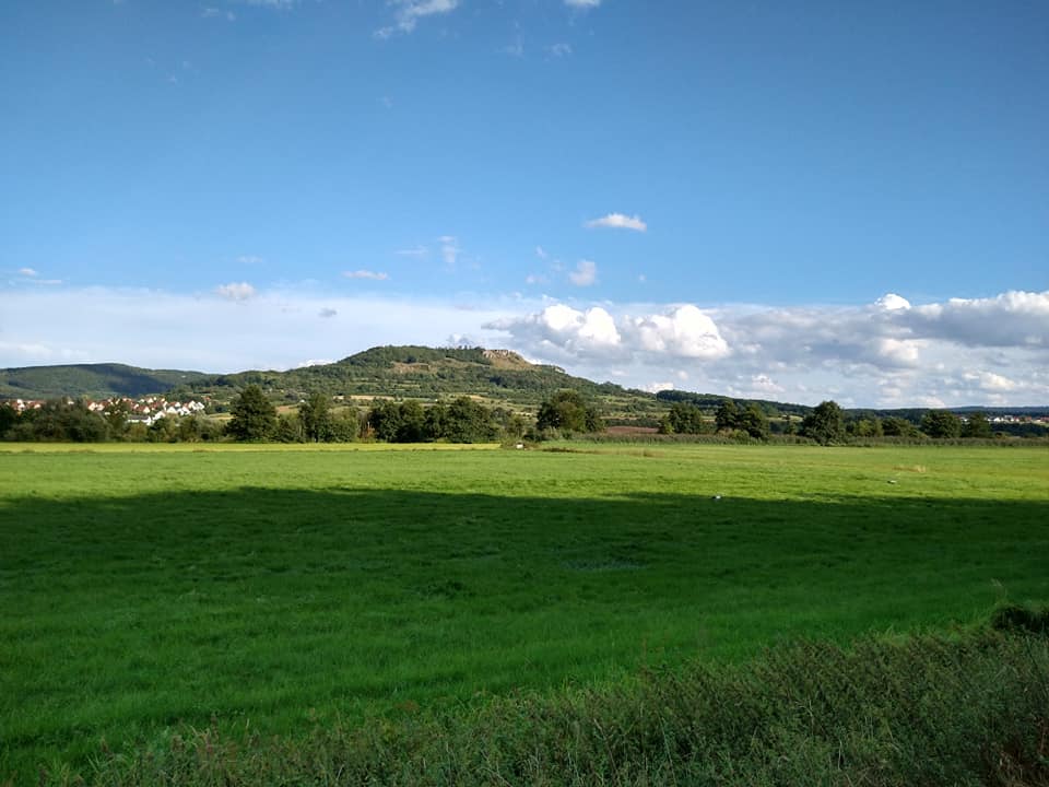
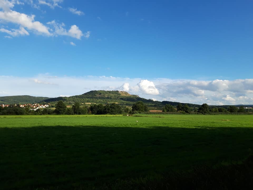
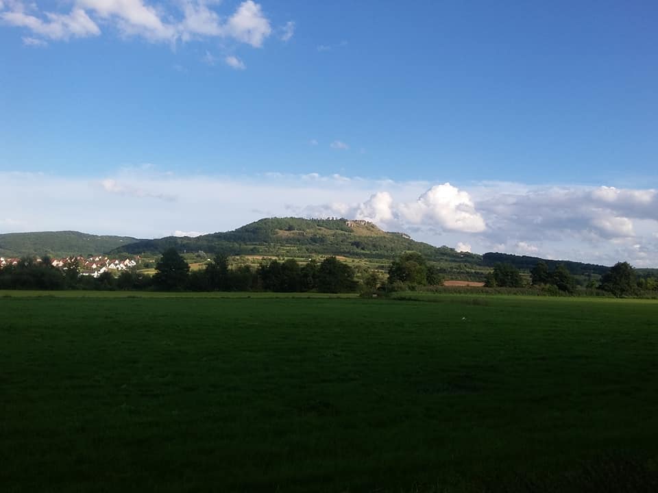
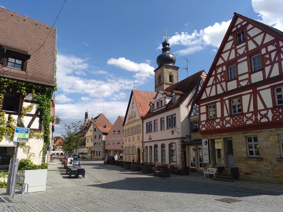
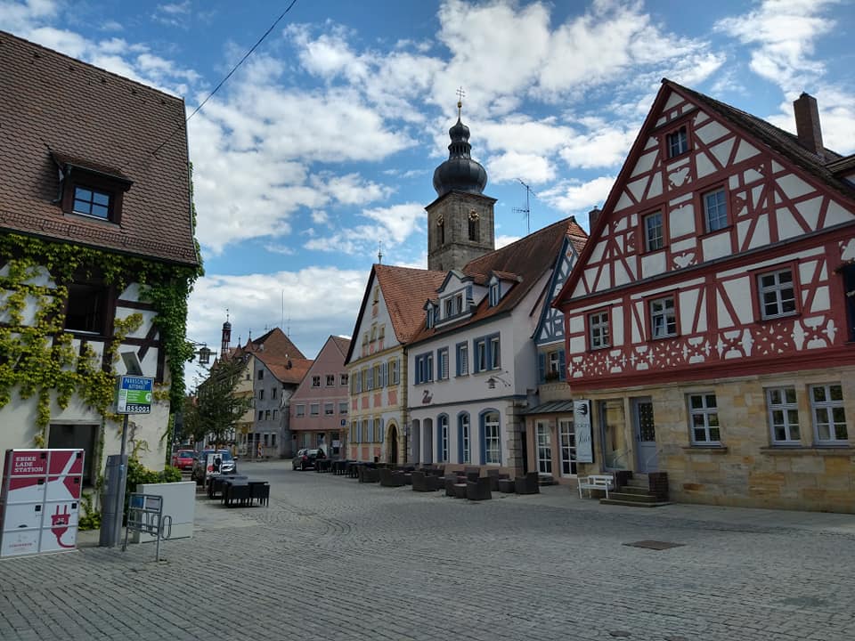
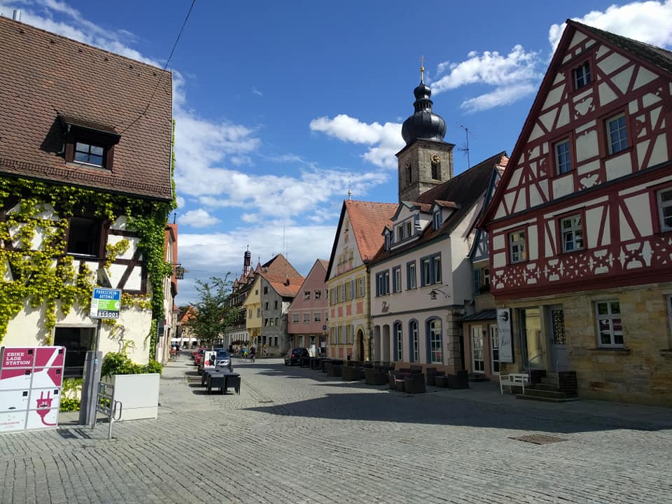
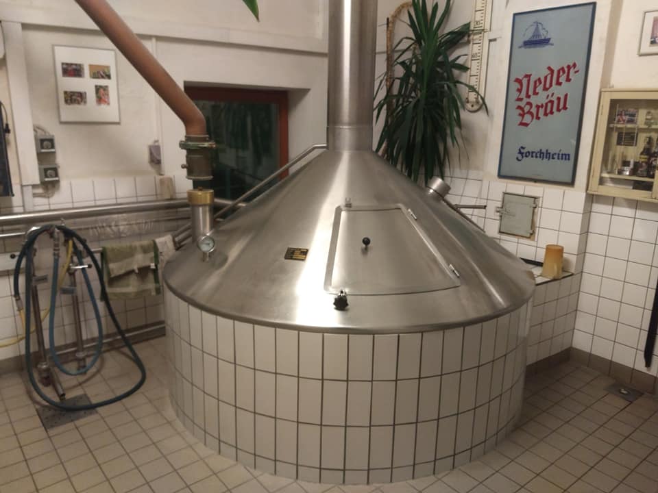
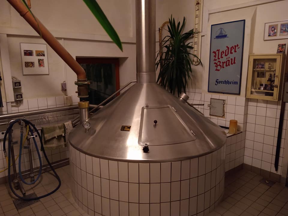
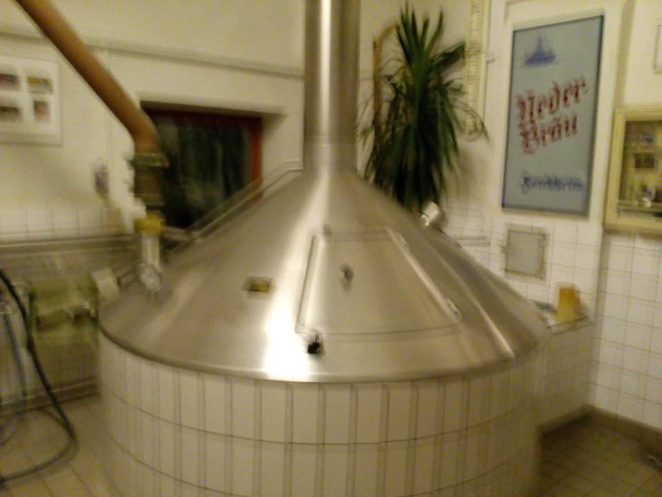
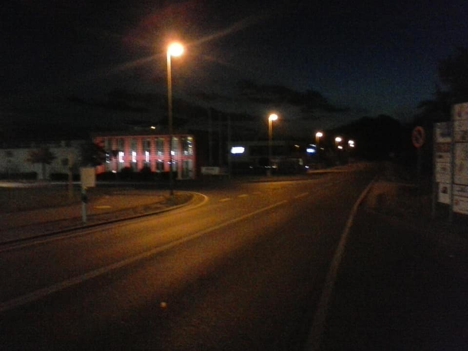
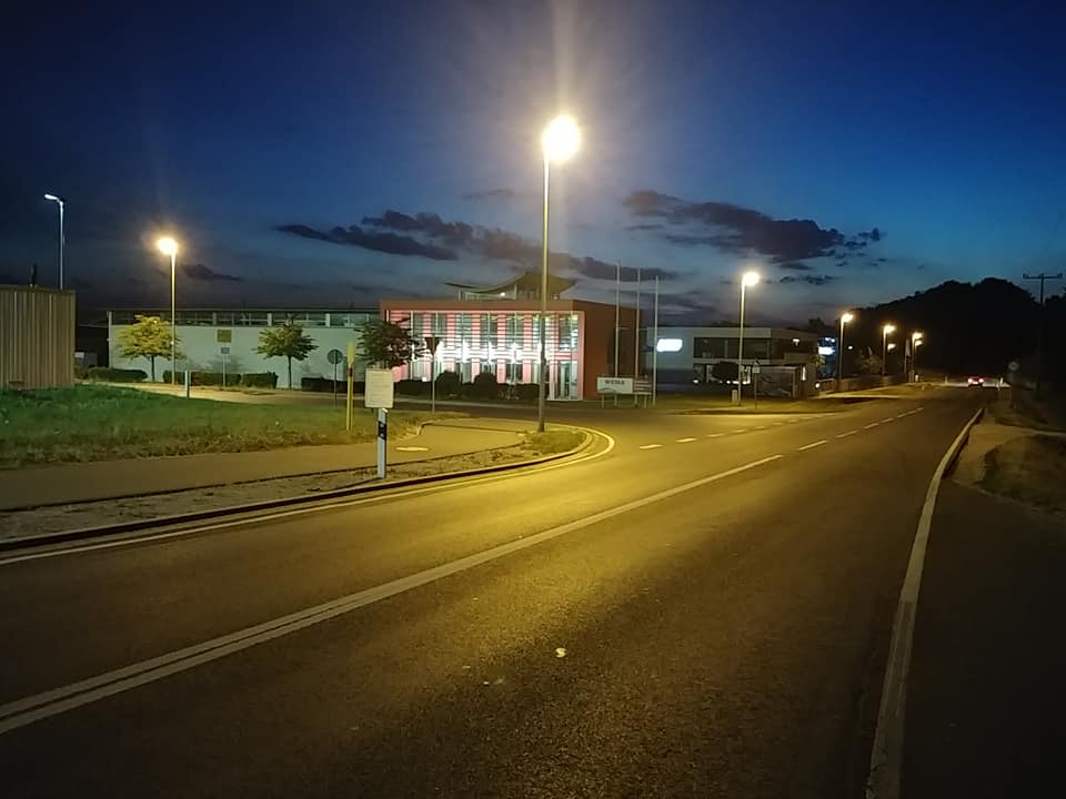
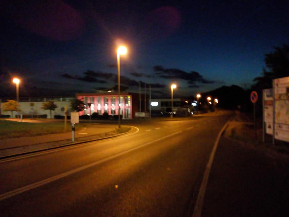
Figure 1: Example images from the Forchheim Image Database

The assessment of the real-world applicability of algorithms requires consistent evaluation protocols with standard benchmark datasets. In 2010, Gloe and Böhme proposed the Dresden Image Database (DIDB) [13], the first large-scale benchmark for camera identification algorithms. It consists of nearly 17,000 images of 73 devices depicting 83 scenes. All devices record the same scenes. This is particularly important for aligning training/test splits with the scene content. Doing so prevents the danger of opening a side channel through scene content, which may lead to overly optimistic results [3, 8].

The DIDB became in the past 10 years one of the most important benchmark datasets in the research community. However, it only consists of DSLR and compact cameras, whereas today most images are recorded with smartphones. Also postprocessed versions of the images from social network sharing are not part of this dataset.

More recently, Shullani et al. proposed VISION [14], an image and video database for benchmarking forensic algorithms. It contains over 34,000 images in total, from 35 smartphones and tablet cameras. A subset of the images has been shared through Facebook and Whatsapp. This enables to investigate the impact of realistic post-processing on forensic traces.

A limitation of VISION is that the images show arbitrary scenes. Thus, a training and evaluation split by scenes is not possible. Moreover, the scene content of images from the same camera are in some cases highly correlated. This may be no issue for methods that strictly operate on noise residuals (e.g., PRNU-based fingerprinting [1]). However, mixed scene content can open a side-channel for end-to-end Convolutional Neural Networks (CNNs), which potentially leads to overly optimistic evaluation results.

In this paper, we propose the Forchheim Image Database (FODB) as a new benchmark that combines the advantages of DIDB and VISION. It consists of 143 scenes, each captured with 27 smartphone cameras. Each image has been shared through the 5 social media apps by Facebook, Instagram, Telegram, Twitter, and Whatsapp. This yields a total of over 23,000 JPEG images. Examples from the database are shown in Fig. 1. FODB allows training/test splits without scene overlap, and simultaneously supports robustness evaluations under real-world post-processing. Hence, it allows rigorous camera association benchmarking on real-world post-processing. To demonstrate the use of the dataset, we perform a benchmark of CNN-based camera identification, which brings insights into relative CNN performances, generalization to unseen post-processing, and performance impacts of scene splitting. In summary, our main contributions are:

• We propose FODB, a new large-scale database for evaluating image forensics algorithms in the wild, which is available at https://faui1-files.cs.fau.de/public/mmsec/datasets/fodb/.

• We employ EfficientNet [15] for camera identification on FODB and show that it signficantly outperforms targeted forensic CNNs across almost all qualities.

• We show that degradation during training sigificantly boosts robustness even for unseen post-processing.

• We demonstrate the importance of scene splitting for learning-based camera identification

The remainder of the paper is organized as follows: We review image provenance benchmarks in Sec. II. The proposed database FODB is described in Sec. III. In Sec. IV, we describe our evaluation protocol for camera identification. The results of this evaluation are presented in Sec. V. Section VI concludes the paper.

II Related Work

In a number of existing datasets, different cameras replicate the same set of scenes. This allows to split the images into training and evaluation subsets such that scenes are disjoint.

The first large-scale forensic benchmark to support such a splitting policy is the Dresden Image Database [13], as stated in the previous section. Cheng et al. propose the NUS dataset [16], with 1,736 images of over 200 scenes, each recorded with 8 DSLR cameras. In another work [17], Cheng et al. recorded additional 944 indoor images. Also in this dataset, each scene is captured with each camera. Although the NUS dataset is presented as an illuminant estimation benchmark, it can directly be used for camera identification, and the acquisition protocols allow scene splitting similar to DIDB. Abdelhamed et al. propose the Smartphone Image Denoising Dataset (SIDD) [18] of about 30,000 images. It consists of 10 indoor scenes under different settings captured with 5 smartphone cameras. The dataset targets image denoising, but can also be used for benchmarking camera identification algorithms with proper scene splitting.

Nowadays, images are often distributed via social networks and by that undergo compression to save memory and bandwidth. Therefore, it is important to assess the performance of forensic algorithms in the presence of such post-processing. Unfortunately, social network sharing has not been relevant during conception of these three datasets. Hence, none of these three datasets comes with images that have already been passed through social networks. While a user of the dataset could in principle pass the images through social networks by herself (given permission by the creators of the datasets), it would still be a remarkably tedious procedure. For example, we estimate that it would require at least a month of work to upload and download the 17,000 images of DIDB through various social networks due to limitations on automated image uploading and downloading on most of their smartphone apps.

In 2018, the IEEE Signal Processing Society hosted a challenge for camera model identification [19], which amongst other aspects addressed algorithm performance under general post-processing. The training dataset consists of 2,750 images of arbitrary scenes from 10 cameras. The test dataset contains original images, as well as images that are recompressed with random JPEG quality, rescaling, or gamma correction. In the VISION database by Shullani et al., around 7,500 images of 35 smartphone cameras have been shared via Facebook in two qualities, and via Whatsapp [14]. It consists of about 30,000 images in 4 qualities levels that enable evaluations of the impact of post-processing. Guidice et al. propose a method for detecting the social network and software used to share an image [20]. To this end, they recorded images with 8 cameras of various types including 4 smartphones. Subsequently, they shared them via 10 social networks and two operating systems (OS) to obtain 2,720 images. Caldelli et al. also investigate social network provenance [10]. They used 1,000 TIFF images from UCID [21], an earlier image retrieval database. These images are compressed with different JPEG qualities and shared on 3 social networks, which results in 30,000 images. However, all images in UCID stem from a single camera, which does not allow for camera identification. Phan et al. investigate traces of instant messenging apps and the host OS. They used 350 images out of 35 devices from the VISION dataset and shared them either once or twice with three messengers and two OSs [11]. This leads to a total of 350 original images, 2,100 single-shared images and 6,300 double-shared images. In a subsequent work, Phan et al. consider up to three-fold sharing on social media platforms [22]. They build two datasets. The first dataset is based on the raw image database RAISE [23]. The images are compressed in JPEG format and shared up to three times on three social networks, which yields a total of 35,100 images. The second dataset is based one based on VISION. Here, 510 images are shared up to three times, to obtain about additional 20,000 images.

The above stated datasets [19, 14, 20, 10, 11, 22] allow benchmarking social network provenance algorithms. With the exception of the dataset by Caldelli et al. which consists of only one source camera [10], they are also suitable for evaluating camera identification algorithms and their robustness for simulated [19] and real-world [14, 20, 11, 22] post-processing. Two further large-scale camera identification benchmarks are SOCRatES [24] and the Daxing Smartphone Identification Dataset (DSID) [25]. SOCRatES contains 9,700 images by 103 smartphones of 60 models, and thus is currently the database with largest number of devices. DSID consists of 43,400 images from 90 devices of 22 models, which currently is to our knowledge the database with the largest number of images and devices per model.

Unfortunately, none of these benchmark datasets supports scene splitting, such that it is currently not possible to investigate social media-related artifacts on split scenes. However, we argue in line with previous works [3, 8] that scene splitting is important during evaluation. It removes by design the threat of leaking side-channel information from the scene content into the evaluation. Such leakage may lead to an overestimation of the performance, as we will show in Sec. V. The proposed Forchheim Image Database FODB closes this gap: it jointly allows a rigorous scene splitting policy, and enables to investigate the effect of social media post-processing on forensic algorithms.

III The Forchheim Image Database

This section describes in detail the cameras, the acquisition protocol, the post-processing and database structure of the proposed dataset. Table I lists the main features of the smartphones. We use a total of of 27 smartphone devices, consisting of 25 different models from 9 brands. It includes two models with more than one device, Samsung Galaxy A6 (devices 15 and 16) and Huawei P9 lite (devices 23 and 25). The smartphones run on Android or iOS and represent older and more recent models (column “Date”) with a wide range of retail prices (not listed). During image acquisition, we only use the main (i.e., rear) camera. All smartphones are configured to store images in JPEG format in the highest available resolution and the highest available JPEG quality. Focus, white-balance and High Dynamic Range (HDR) imaging is set to automatic mode, where applicable.

All 143 scenes are captured in or near the town of Forchheim, Germany; hence the name Forchheim Image Database. Each camera recorded one image per scene. 10 images are missing or excluded due to technical or privacy issues, resulting in a total of $3,861-10=3,851$ images. To assert diverse image content, we mix indoor and outdoor, day and night, close-up and distant, and natural and man-made scenes. Examples are shown in Fig. 1.

TABLE I: Main features of smartphones in FODB

ID	Brand	Model	OS	Version	Date
01	Motorola	E3	Android	6.0	09/2016
02	LG	Optimus L50	Android	4.4.2	06/2010
03	Wiko	Lenny 2	Android	5.1	09/2014
04	LG	G3	Android	5.0	07/2014
05	Apple	iPhone 6s	iOS	13.6	09/2015
06	LG	G6	Android	9	05/2017
07	Motorola	Z2 Play	Android	8.0.0	08/2017
08	Motorola	G8 Plus	Android	9	10/2019
09	Samsung	Galaxy S4 mini	Android	4.4.4	05/2013
10	Samsung	Galaxy J1	Android	4.4.4	01/2015
11	Samsung	Galaxy J3	Android	5.1.1	01/2016
12	Samsung	Galaxy Star 5280	Android	4.1.2	05/2013
13	Sony	Xperia E5	Android	6.0	11/2016
14	Apple	iPhone 3	iOS	7.1.2	06/2008
15	Samsung	Galaxy A6	Android	10	05/2018
16	Samsung	Galaxy A6	Android	10	05/2018
17	Apple	iPhone 7	iOS	12.3.1	09/2016
18	Samsung	Galaxy S4	Android	6.0.1	04/2013
19	Apple	iPhone 8 Plus	iOS	13.2	09/2017
20	Google	Pixel 3	Android	9	11/2018
21	Google	Nexus 5	Android	8.1.0	10/2015
22	BQ	Aquaris X	Android	8.1.0	05/2017
23	Huawei	P9 lite	Android	6.0	05/2016
24	Huawei	P8 lite	Android	5.0	04/2015
25	Huawei	P9 lite	Android	7.0	05/2016
26	Huawei	P20 lite	Android	8.0.0	04/2018
27	Google	Pixel XL	Android	10	10/2016

We refer to camera-native images as original (orig.). Additionally, we created five post-processed versions of each image. For this, we installed the apps Facebook, Instagram, Telegram, Twitter and Whatsapp on each device and manually shared all images. In the Facebook app, we uploaded the images of each device to a dedicated photo album in default quality. Then, we used the functionality to download entire albums in the browser version of Facebook. During upload on Instagram, a user must select a square crop from an image, and optionally a filter. We uploaded all images with default settings for cropping, resulting in a center crop, and disabled any filters. For download we used the open source tool “Instaloader” (Version 4.5.2). In the Twitter app, all images were uploaded without filter, and downloaded via the Firefox browser plugin “Twitter Media Downloader” (Version 0.1.4.16). For Telegram and Whatsapp, the images of each device were sent to device 6 (LG G6), except for the images of device 6 itself, which were sent to device 8 (Motorola G8 Plus). In this way, the database contains a total of $6\cdot(27\cdot 143-10)=$23\,106$$ JPEG images.

Social network and messenger sharing was executed one device after another, to avoid confounding images of different devices. During sharing, the social networks and messengers non-trivially modify the image filenames, and metadata is largely removed. For re-identifying the shown scene, we correlated the original and post-processed images for each device individually. The originals were first downscaled to match the size of the post-processed versions, and, in case of Instagram, center cropped prior to downscaling. Only very few cases were ambiguouos, which were manually labeled.

The database is hierarchically organized: at root level, images from each device are in one directory D$\langle$ID$\rangle$_$\langle$Brand$\rangle$_$\langle$Model$\rangle$_$\langle$i$\rangle$, where ID, Brand and Model are substituted according to Tab. I, and i $\in\{1,2\}$ enumerates the devices of a model. Each directory contains six provenance subdirectories orig, facebook, instagram, telegram, twitter and whatsapp. These directories contain the images of device ID, provenance prov and scene ID scene with the pattern D$\langle$ID$\rangle$_img_$\langle$prov$\rangle$_$\langle$scene$\rangle$.jpg, for example D06_img_twitter_0030.jpg.

IV Camera Identification: Dataset Split, Methods, and Training Augmentation

We demonstrate an application of FODB by studying the behavior of CNNs for camera identification. This section briefly describes the used methods and their training.

IV-A Dataset Splits

To create training, validation and test data, we split the set of 143 scenes $\mathcal{S}$ of FODB into three disjoint sets $\mathcal{S}^{\mathrm{train}}$, $\mathcal{S}^{\mathrm{val}}$ and $\mathcal{S}^{\mathrm{test}}$, and we set $\lvert\mathcal{S}^{\mathrm{train}}|=97$, $\lvert\mathcal{S}^{\mathrm{val}}|=18$, $\lvert\mathcal{S}^{\mathrm{test}}|=28$. For camera models with more than one device, we choose the device with the smallest ID, which yields $N_{\mathcal{K}}=25$ cameras, and hence $25$ classes. Thus we obtain $\lvert\mathcal{S}^{\mathrm{train}}\rvert\cdot N_{\mathcal{K}}=2425$ training, $\lvert\mathcal{S}^{\mathrm{val}}\rvert\cdot N_{\mathcal{K}}=450$ validation and $\lvert\mathcal{S}^{\mathrm{test}}\rvert\cdot N_{\mathcal{K}}=700$ test images per post-processing quality.

IV-B Compared Methods

We reimplemented three CNN-based forensic methods for source camera identification. First, the method by Bondi et al., which we subsequently refer to as “BondiNet” [8]. Second, MISLnet by Bayar et al. [26] in its improved version as the feature extractor in the work by Mayer et al. [27] by the same group. Third, RemNet by Rafi et al. [9], which has been presented at the IEEE Signal Processing Cup 2018. We additionally report results on EfficientNet-B5, a recently proposed general-purpose CNN from the field of computer vision [15]. All models are trained with crossentropy loss.

The input patch size of each CNN except MISLNet is set to $64\times 64$ pixels. The outputs of the CNNs are adapted to distinguish $N_{\mathcal{K}}=25$ classes. Note that the classes are balanced, and random guessing accuracy is $N_{\mathcal{K}}^{-1}$, i.e., $4\%$, on all experiments on FODB.

Initial experiments with BondiNet using the parameters of the paper [8] led to poor validation performance on FODB. Hence, we evaluate BondiNet for the following set of hyperparameters, which led to significantly better validation results: Adam optimizer with $\alpha=10^{-3}$, $\beta_{1}=0.9$ and $\beta_{2}=0.999$, no weight decay, additional batch normalization after each convolution, and direct classification using CNN outputs instead of using an SVM. For MISLnet, we reimplemented the improved version of the same group [27]. The patch input size is $256\times 256$ pixels, and hence somewhat larger than for the remaining networks. We address this in the patch clustering described below. For RemNet, we reimplemented the implementation as described in the paper.

For EfficientNet-B5, we use weights pretrained on ImageNet [28], and remove the final classification layer of the pretrained network. Then, we add global average pooling and a dense layer with $N_{\mathcal{K}}=25$ output units and softmax activation. The weights of the new classification layer are set with Glorot uniform initialization [29]. During all experiments, we use Adam optimization [30] with learning rate $\alpha=10^{-3}$ and moments $\beta_{1}=0.9$ and $\beta_{2}=0.999$. Whenever the validation loss stagnates for two consecutive epochs, the learning rate is halved, and we apply early stopping.

To accomodate for differences in the input resolution of the networks, we adopt the patch cluster strategy by Rafi et al. [9]. To this end, we consider an image area of $256\times 256$ pixels as a patch cluster. A patch cluster is considered to be non-informative if it mostly consists of homogeneous pixels, which is determined by a heuristic quality criterion used by Bondi et al. [31, Eqn. (1)] and Rafi et al. [9, Eqn. (7)],

$$Q(P)=\frac{1}{3}\sum\limits_{c\in\{R,G,B\}}\alpha\beta(\mathbf{\mu}_{c}-\mathbf{\mu}_{c}^{2})+(1-\alpha)(1-\exp(\gamma\sigma_{c}))\enspace,$$ (1)

where $\mathbf{\mu}_{c}$ and $\sigma_{c}$ denote the patch cluster mean and standard deviation in the red, green, and blue color channels $c$, and $\alpha=0.7$, $\beta=4$, $\gamma=\ln(0.01)$.

IV-C Matching the Network Input Resolutions

For evaluation, it is important to provide to each algorithm the same amount of information. Thus, for both training and testing, we subdivide the image into non-overlapping $256\times 256$ patch cluster candidates, and sort them by the quality criterion $Q(P)$. The top $100$ candidates are used as patch clusters for the image.

For training, each selected patch cluster is used once per training epoch. MISLnet obtains full patch clusters to match its $256\times 256$ pixel inputs. The remaining networks obtain a randomly selected $64\times 64$ pixels subwindow per cluster to match their input size. For validation, we use the same approach but with fixed random seed to achieve a consistent comparison throughout all epochs.

For testing, we also feed a full $256\times 256$ patch cluster to MISLnet. For the remaining networks, we subdivide a patch cluster into $16$ non-overlapping patches of $64\times 64$ pixels.

These results are used to report three metrics: camera identification accuracies on individual $64\times 64$ patches (excluding MISLnet), accuracies on patch clusters of $256\times 256$ pixels, and accuracies for the whole image. For the per-cluster accuracies, we directly calculate the accuracy for MISLnet’s $256\times 256$ prediction. For the remaining networks, the patch cluster prediction $\hat{k}$ is calculated via soft majority voting over all $64\times 64$ patch predictions,

$$\hat{k}=\operatorname*{argmax}\limits_{k}\sum\limits_{i\in\mathcal{I}}y_{i}^{k}\enspace,$$ (2)

where $y_{i}^{k}$ denotes the $k$-th component of the CNN output for the $i$-th patch in the cluster. The prediction for the whole image is analogously calculated via soft majority voting over all individual CNN outputs on that image.

IV-D Training Augmentation

Throughout all training runs, we randomly apply horizontal flipping, vertical flipping, and rotation by integer multiples of $90^{\circ}$, with equal probability for each case.

For a subset of the experiments, we additionally apply artificial degradations during training to increase the robustness of all CNNs against post-processing. Prior to flipping or rotation, we rescale a training patch cluster with probability $0.9$. The rescaling factor is randomly drawn from a discrete distribution over the interval $[0.25,\ldots,4]$. In order to make upsampling and downsampling equally likely, we rewrite the interval as $[0.25=2^{-2},\ldots,2^{j},\ldots,4=2^{2}]$ and subdivide the exponent $j$ in $50$ equally spaced samples. We draw from these exponents with uniform probability. After flipping or rotation, we extract a patch from the (rescaled or non-rescaled) cluster, and recompress it in JPEG format with probability $0.9$. The JPEG quality factor is uniformly chosen from $[100,90,\dots,10]$.

For the rather challenging experiments in Sec. V-C and Sec. V-D, we try to maximize the performance of RemNet and EfficientNet-B5 by pretraining on DIDB’s 18 cameras. To this end, we use the DIDB training/validation split by Bondi et al. [8]. Considering our four variants of RemNet and EfficientNet-B5 with and without artificial degradations, we investigate possible gains in validation performance when pre-training on DIDB. We apply artificial degradations on DIDB only if the subsequent training on FODB also uses artificial degradations, in order to have these degradations either throughout the whole training process or not at all. We then select for the experiments either the variant with DIDB-pretraining or without depending on the validation loss. The results are listed in Tab. II. Boldface shows validation loss and accuracy of the selected model. The column indicating validation on FODB is used in Sec. V-C, the column indicating validation on VISION in Sec. V-D.

TABLE II: Averaged overall validation performance for FODB and VISION, with and without pretraining on DIDB. Boldface shows the selected model variants based on validation loss.

			Validation Dataset
Training Parameters			FODB		VISION
Model	Degr.	Pretr.	Loss	Acc.	Loss	Acc.
RemNet	no	no	0.1870	92.72	0.1898	93.90
RemNet	no	yes	0.1885	92.86	0.1731	94.49
RemNet	yes	no	2.4268	31.06	1.9586	42.67
RemNet	yes	yes	2.5735	26.07	1.9295	43.47
EN-B5	no	no	0.1176	95.79	0.1465	95.91
EN-B5	no	yes	0.1178	95.62	0.1265	96.22
EN-B5	yes	no	1.6894	52.12	1.2410	63.68
EN-B5	yes	yes	1.6756	52.77	1.2179	64.35

(a)

(b)

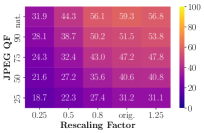
(c)

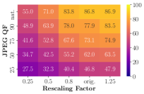
(d)

(e)

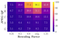
(f)

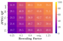
(g)

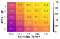
(h)

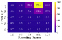
(i) RemNet, no degr.

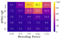
(j) EfficientNet-B5, no degr.

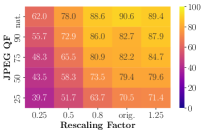
(k) RemNet, degr.

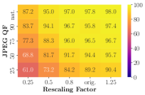
(l) EfficientNet-B5, degr.

Figure 2: Robustness against rescaling and JPEG recompression for predictions per patch (first row), cluster (second row) and image (third row). Columns (a) and (b) show RemNet and EfficientNet-B5 accuracies without augmentation of degradations during training. Columns (c) and (d) show RemNet and EfficientNet-B5 accuracies with augmentation of degradations during training.

V Results

V-A Performance Under Ideal Conditions

In this experiment, we benchmark CNNs for camera identification under ideal conditions without any post-processing. During training, we only augment with flipping and rotation, but not with resizing or JPEG recompression.

Table III shows the per-patch, per-cluster and per-image accuracies for the original (camera-native) test images of FODB. EfficientNet-B5 consistently outperforms the other CNNs for patches and clusters with accuracies of $96.3\%$ and $98.1\%$, respectively. For image-level classification, RemNet and EfficientNet-B5 are on par with an accuracy of $99.1\%$. Majority voting improves individual predictions across all CNNs, which indicates some degree of statistical independence of the prediction errors.

TABLE III: Accuracy (in percent) for closed-set camera identification on camera-native FODB test images.

CNN	Patch	Cluster	Image
BondiNet[8]	71.4	84.9	93.1
MISLnet [27]	-	93.5	96.8
RemNet [9]	93.8	96.6	99.1
EfficientNet-B5 [15]	96.3	98.1	99.1

V-B Robustness Against Known Post-Processing

In this experiment, we take a closer look at the two best performing CNNs on clean images, RemNet and EfficientNet-B5, and evaluate their robustness against post-processing. For this, we determine the test accuracy on FODB for all combinations of rescaling with factors $f_{\mathrm{test}}\in\{0.25,0.5,0.8,\mathrm{orig.},1.25\}$ and JPEG recompression with quality factors $\mathrm{QF}_{\mathrm{test}}\in\{\mathrm{nat.},90,75,50,25\}$. $\mathrm{orig.}$ (original), resp. $\mathrm{nat.}$ (native) indicates no rescaling and no JPEG recompression. Note that rescaling is applied to patch clusters prior to patch extraction, which quadratically scales the number of patches for majority voting on patch clusters and images with $f_{\mathrm{test}}$.

Figure 2i and Fig. 2j show the accuracies for RemNet and EfficientNet-B5. From top to bottom are accuracies on patch level, cluster level, and image level. Throughout all qualities, EfficientNet-B5 outperforms RemNet. In most cases, majority voting again increases the accuracy. While accuracies for both CNNs are almost perfect for camera-native images ($\mathrm{orig.}$, $\mathrm{nat.}$) with $99.1\%$, it rapidly decreases on post-processed images. This is not surprising, since only high quality images are used for training. The CNNs likely rely on fragile high-frequent traces, which are attenuated by postprocessing [32].

We retrain both CNNs with artificial degradations as described in Sec. IV-D to improve the robustness against post-processing. The results for these retrained CNNs are shown in Fig. 2k and Fig. 2l. Already at patch-level, the accuracies of both CNNs are much more stable compared to training without degradations. For example, at $f_{\mathrm{test}}=0.5$, $\mathrm{QF}_{\mathrm{test}}=75$, the test accuracies at patch-level amount to $32.4\%$ and $52.8\%$ for both CNNs, compared to $5.1\%$ and $7.6\%$ without these augmentations. Moreover, EfficientNet-B5 remarkably outperforms RemNet. For example, the patch-level performance on clean images, is $56.1\%$ for RemNet and $83.8\%$ for EfficientNet-B5. For both CNNs, majority voting further significantly improves the performance. For image-level decisions and camera-native images, the performance of EfficientNet-B5 trained with degradations ($97.0\%$) is close to testing without degradations ($99.1\%$). RemNet has difficulties to fully benefit from augmentation with degraded images, with accuracies dropping from $99.1\%$ without degradations to $88.6\%$ with degradations. We hypothesize that this difference can in part be attributed to the significantly larger capacity of EfficientNet-B5: while both CNNs perform comparably on the easier task of clean images, a CNN with larger capacity might be required for additionally learning the traces of degraded images. Still, also the superior EfficientNet-B5 shows an accuracy-robustness trade-off, a phenomenon that has been observed for adversarial training before [32, 33].

V-C Robustness Against Unknown Real-World Post-Processing

TABLE IV: Test accuracies on FODB for camera-native and post-processed images. Top: boldface shows the best accuracy per column for unknown post-processing. Bottom: blue shows the oracle performance for known post-processing at training.

			Test Dataset
Training Parameters			orig		FB		IG		TG		TW		WA
CNN	Dataset	Degr.	patch	image	patch	image	patch	image	patch	image	patch	image	patch	image
RemNet	orig	no	93.8	99.1	4.0	3.6	4.2	4.2	4.5	4.3	5.5	4.7	4.2	3.9
RemNet	orig	yes	59.3	90.6	18.4	36.0	22.9	48.9	26.2	52.8	37.3	74.2	24.2	50.8
EN-B5	orig	no	96.3	99.1	4.9	4.6	5.7	5.6	5.7	5.3	10.8	9.8	7.0	6.8
EN-B5	orig	yes	86.5	98.0	27.7	51.1	35.4	67.5	42.2	73.1	60.7	93.2	38.5	72.9
EN-B5	FB	no	13.8	23.6	38.4	71.4	29.1	51.1	28.5	44.2	23.8	38.3	30.8	54.7
EN-B5	IG	no	8.1	9.4	28.4	52.1	52.1	84.0	13.5	14.0	12.1	14.0	40.4	69.1
EN-B5	TG	no	16.7	23.3	21.1	32.4	25.5	37.6	57.2	86.2	35.4	55.0	32.8	51.5
EN-B5	TW	no	36.4	57.1	14.7	21.9	25.6	41.9	28.2	41.6	76.2	97.7	33.6	54.2
EN-B5	WA	no	17.3	27.3	28.8	52.4	41.5	69.2	31.0	45.3	28.4	38.3	60.0	90.4

TABLE V: Test accuracies on VISION for camera-native and post-processed images. Top: boldface shows the best accuracy per column for unknown post-processing. Bottom: blue shows the oracle performance for known post-processing at training. LQ and HQ denote low quality and high quality.

			Test Dataset
Training Parameters			orig		FB (LQ)		FB (HQ)		WA
Archit.	Dataset	Degr.	patch	image	patch	image	patch	image	patch	image
RemNet	orig	no	93.9	98.6	4.6	4.1	6.4	7.2	9.2	12.8
RemNet	orig	yes	64.7	86.7	34.8	64.0	41.5	73.9	45.7	75.9
EN-B5	orig	no	95.9	99.2	4.9	5.9	8.3	8.7	10.2	11.8
EN-B5	orig	yes	88.4	97.0	46.3	77.0	57.7	88.4	66.5	92.4
EN-B5	FB (LQ)	no	8.8	14.3	64.6	88.5	22.3	33.0	28.9	40.7
EN-B5	FB (HQ)	no	31.7	43.7	27.4	39.9	72.8	95.4	25.4	36.8
EN-B5	WA	no	21.6	32.9	30.5	47.5	18.3	27.8	77.3	96.3

TABLE VI: Test accuracies for splits on sorted images of VISION for camera-native and post-processed images. Top: boldface indicates the best accuracy per column for unknown post-processing. Bottom: blue indicates the oracle performance for known post-processing. LQ and HQ denote low quality and high quality.

			Test Dataset
Training Parameters			orig		FB (LQ)		FB (HQ)		WA
Archit.	Dataset	Degr.	patch	image	patch	image	patch	image	patch	image
RemNet	orig	no	87.5	93.2	3.7	4.8	4.7	5.5	5.5	7.4
RemNet	orig	yes	44.2	67.9	20.1	39.5	25.8	52.4	27.9	51.7
EN-B5	orig	no	87.8	93.9	3.6	4.5	7.0	7.4	6.9	8.6
EN-B5	orig	yes	76.8	88.5	28.2	54.1	40.9	70.5	44.7	72.4
EN-B5	FB (LQ)	no	7.3	10.8	42.3	67.6	16.8	26.3	20.7	29.1
EN-B5	FB (HQ)	no	26.3	39.0	18.0	26.0	55.2	83.7	16.1	21.6
EN-B5	WA	no	18.7	30.7	19.4	30.8	14.4	21.8	56.1	82.2

In this section, we evaluate the robustness of RemNet and EfficientNet-B5 against real-world post-processing by unknown algorithms and parameters, as it occurs during social network sharing. We again train both CNNs once without and once with degradations. The networks do not obtain examples of social media images for training.

We evaluate the selected models on original images and all five post-processed versions of the test images (Facebook: FB, Instagram: IG, Telegram: TG, Twitter: TW, Whatsapp: WA). The resulting accuracies are listed in Tab. IV. When training without degradations, the networks can only excell on original images, analogously to the previous experiments. Pretraining on DIDB slightly improves the performance of EfficientNet-B5 on clean images. Augmentation with artificial degradations significantly improves the performance of both CNNs on all social network data, eventhough social media data itself was not part of the training. Again, EfficientNet-B5 largely outperforms RemNet in all experiments.

We perform an additional experiment as a reference for the impact of prior knowledge on the data: we pretrained EfficientNet-B5 on DIDB with degradations. Additionally, we feed the social network images from the training set to EfficientNet-B5 as an oracle for the test set degradations. Table IV (bottom) shows that such strong prior knowledge yields at image level accuracy gains from $4.5~{}\mathrm{p.p.}$ for Twitter (with baseline already $93.2\%$) up to $20.3~{}\mathrm{p.p.}$ for Facebook.

V-D Impact of Scene Splitting

In this experiment, we analyze the influence of scene splitting on CNN-based camera identification on the VISION dataset. The scene content is not constrained in several datasets including VISION which prevents splitting by scenes. Some per-device image sets in VISION are highly correlated, such that randomized splitting makes it likely that training and test sets contain images of identical cameras with similar content. We conjecture that scene content may open a side-channel that CNNs are prone to exploit, which may lead to an overestimation of the CNN generalization. We show empirical evidence for this conjecture in two experiments.

First, we randomly split the VISION images in training, validation and test sets. We use the evaluation protocol by Marra et al. [34] and use the $29$ unique devices with random guessing accuracy of $29^{-1}=3.45\%$.

Second, we make an attempt to improve the splitting strategy, and to further separate image content between training and test set. To this end, we sort the images of each device by their acquisition time using DateTimeOriginal from the EXIF file header, and split the dataset along the timeline of the images. In this way, similar images recorded within a short period of time are likely to be either in the training or test set, but not in both. This significantly reduces overlap in image content between training and test set. Except of the splitting policy, all settings are identical between both experiments.

Results for the first and second experiment are shown in Tab. V and Tab. VI. Performances drop significantly when moving from completely random splits (Tab. V) to splits by timestamp (Tab. VI). For example, on clean images the accuracy of EfficientNet-B5 without degradation drops from $99.2\%$ to $93.9\%$. The performance of EfficientNet-B5 with degradation for Whatsapp-compressed test images drops even by $20~{}\mathrm{p.p.}$, from $92.4\%$ to $72.4\%$. This discrepancy suggests that scene content contributes to the results in Tab. V. Moreover, such a side-channel may prevent the CNN from learning more relevant traces. We hence believe that the results in Tab. VI are closer to the performance that can be expected in practice. These observations emphasize the importance of a rigorous scene splitting as supported by FODB.

VI Conclusion

This work proposes the Forchheim Image Database (FODB) as a new benchmark for image forensics algorithms under real-world post-processing. Our database consists of more than 23,000 images of 143 scenes by 27 smartphone devices of 25 models and 9 brands. FODB combines clean training/validation/test data splits by scene with a wide range of modern smartphone devices shared through a total of five social network sites, which allows rigorous evaluations of forensic algorithms on real-world image distortions. We demonstrate FODB’s usefulness in an evaluation on the task of camera identification. Our results provide three insights. First, the general-purpose network EfficientNet-B5 largely outperforms three specialized CNNs. Second, EfficientNet-B5’s large capacity also fully benefits from training data augmentation to generalize to unseen degradations. Third, clean data splits by scenes can help to better predict generalization performance.

References

- [1] J. Lukas, J. Fridrich, and M. Goljan, “Digital Camera Identification from Sensor Pattern Noise,” IEEE Transactions on Information Forensics and Security, pp. 205–214, 2006.
- [2] H. Farid, “A Survey of Image Forgery Detection,” IEEE Signal Processing Magazine, pp. 16–25, 2009.
- [3] M. Kirchner and T. Gloe, “Forensic Camera Model Identification,” in Handbook of Digital Forensics of Multimedia Data and Devices, 2015, pp. 329–374.
- [4] P. Yang, D. Baracchi, R. Ni, Y. Zhao, F. Argenti, and A. Piva, “A Survey of Deep Learning-Based Source Image Forensics,” Journal of Imaging, p. 9, 2020.
- [5] M. Huh, A. Liu, A. Owens, and A. A. Efros, “Fighting Fake News: Image Splice Detection Via Learned Self-Consistency,” in European Conference on Computer Vision, 2018, pp. 101–117.
- [6] P. Zhou, X. Han, V. I. Morariu, and L. S. Davis, “Learning Rich Features for Image Manipulation Detection,” in IEEE Conference on Computer Vision and Pattern Recognition, 2018, pp. 1053–1061.
- [7] D. Cozzolino and L. Verdoliva, “Noiseprint: A CNN-Based Camera Model Fingerprint,” IEEE Transactions on Information Forensics and Security, pp. 144–159, 2019.
- [8] L. Bondi, L. Baroffio, D. Guera, P. Bestagini, E. J. Delp, and S. Tubaro, “First Steps Toward Camera Model Identification With Convolutional Neural Networks,” IEEE Signal Process. Lett., pp. 259–263, 2017.
- [9] A. M. Rafi, T. I. Tonmoy, U. Kamal, Q. J. Wu, and M. K. Hasan, “RemNet: Remnant Convolutional Neural Network for Camera Model Identification,” Neural Computing and Applications, pp. 1–16, 2020.
- [10] R. Caldelli, R. Becarelli, and I. Amerini, “Image Origin Classification Based on Social Network Provenance,” IEEE Transactions on Information Forensics and Security, pp. 1299–1308, 2017.
- [11] Q.-T. Phan, C. Pasquini, G. Boato, and F. G. De Natale, “Identifying Image Provenance: An Analysis of Mobile Instant Messaging Apps,” in IEEE International Workshop on Multimedia Signal Processing, 2018, pp. 1–6.
- [12] D. Moreira, A. Bharati, J. Brogan, A. Pinto, M. Parowski, K. W. Bowyer, P. J. Flynn, A. Rocha, and W. J. Scheirer, “Image Provenance Analysis at Scale,” IEEE Transactions on Image Processing, pp. 6109–6123, 2018.
- [13] T. Gloe and R. Böhme, “The Dresden Image Database for Benchmarking Digital Image Forensics,” J. Digital Forensic Practice, pp. 150–159, 2010.
- [14] D. Shullani, M. Fontani, M. Iuliani, O. A. Shaya, and A. Piva, “VISION: A Video And Image Dataset for Source Identification,” EURASIP J. Inf. Secur., vol. 2017, p. 15, 2017.
- [15] M. Tan and Q. Le, “EfficientNet: Rethinking Model Scaling for Convolutional Neural Networks,” in International Conference on Machine Learning, 2019, pp. 6105–6114.
- [16] D. Cheng, D. K. Prasad, and M. S. Brown, “Illuminant Estimation for Color Constancy: Why Spatial-Domain Methods Work and the Role of the Color Distribution,” JOSA A, pp. 1049–1058, 2014.
- [17] D. Cheng, B. Price, S. Cohen, and M. S. Brown, “Beyond White: Ground Truth Colors for Color Constancy Correction,” in IEEE International Conference on Computer Vision, 2015, pp. 298–306.
- [18] A. Abdelhamed, S. Lin, and M. S. Brown, “A High-Quality Denoising Dataset for Smartphone Cameras,” in IEEE Conference on Computer Vision and Pattern Recognition, 2018, pp. 1692–1700.
- [19] “IEEE’s Signal Processing Society - Camera Model Identification,” https://www.kaggle.com/c/sp-society-camera-model-identification, 2018, online. Accessed: Sept. 26, 2020.
- [20] O. Giudice, A. Paratore, M. Moltisanti, and S. Battiato, “A Classification Engine for Image Ballistics of Social Data,” in International Conference on Image Analysis and Processing, 2017, pp. 625–636.
- [21] G. Schaefer and M. Stich, “UCID: An Uncompressed Color Image Database,” in Storage and Retrieval Methods and Applications for Multimedia, 2003, pp. 472–480.
- [22] Q.-T. Phan, G. Boato, R. Caldelli, and I. Amerini, “Tracking Multiple Image Sharing on Social Networks,” in IEEE International Conference on Acoustics, Speech and Signal Processing, 2019, pp. 8266–8270.
- [23] D.-T. Dang-Nguyen, C. Pasquini, V. Conotter, and G. Boato, “RAISE: A Raw Images Dataset for Digital Image Forensics,” in ACM Multimedia Systems Conference, 2015, pp. 219–224.
- [24] C. Galdi, F. Hartung, and J.-L. Dugelay, “SOCRatES: A Database of Realistic Data for SOurce Camera REcognition on Smartphones.” in ICPRAM, 2019, pp. 648–655.
- [25] H. Tian, Y. Xiao, G. Cao, Y. Zhang, Z. Xu, and Y. Zhao, “Daxing Smartphone Identification Dataset,” IEEE Access, pp. 101 046–101 053, 2019.
- [26] B. Bayar and M. C. Stamm, “Constrained Convolutional Neural Networks: A New Approach Towards General Purpose Image Manipulation Detection,” IEEE Transactions on Information Forensics and Security, pp. 2691–2706, 2018.
- [27] O. Mayer and M. C. Stamm, “Forensic Similarity for Digital Images,” IEEE Transactions on Information Forensics and Security, pp. 1331–1346, 2019.
- [28] J. Deng, W. Dong, R. Socher, L.-J. Li, K. Li, and L. Fei-Fei, “ImageNet: A Large-Scale Hierarchical Image Database,” in 2009 IEEE conference on computer vision and pattern recognition, 2009, pp. 248–255.
- [29] X. Glorot and Y. Bengio, “Understanding the Difficulty of Training Deep Feedforward Neural Networks,” in International Conference on Artificial Intelligence and Statistics, 2010, pp. 249–256.
- [30] D. P. Kingma and J. Ba, “Adam: A Method for Stochastic Optimization,” in International Conference on Learning Representations, 2015.
- [31] L. Bondi, D. Güera, L. Baroffio, P. Bestagini, E. J. Delp, and S. Tubaro, “A Preliminary Study on Convolutional Neural Networks for Camera Model Identification,” Electronic Imaging, pp. 67–76, 2017.
- [32] D. Tsipras, S. Santurkar, L. Engstrom, A. Turner, and A. Madry, “Robustness May Be at Odds with Accuracy,” arXiv preprint, 2018.
- [33] A. Raghunathan, S. M. Xie, F. Yang, J. C. Duchi, and P. Liang, “Adversarial Training Can Hurt Generalization,” arXiv preprint, 2019.
- [34] F. Marra, D. Gragnaniello, and L. Verdoliva, “On the Vulnerability of Deep Learning to Adversarial Attacks for Camera Model Identification,” Signal Process. Image Commun., pp. 240–248, 2018.