BCH short = BCH, long= Bose-Chaudhuri-Hocquenghem \DeclareAcronymBER short = BER, long= bit error rate \DeclareAcronymBLER short = BLER, long= block error rate \DeclareAcronymBP short = BP, long = belief propagation \DeclareAcronymCN short = CN, long = check node \DeclareAcronymNBPD short = NBP-D, long = neural belief propagation with decimation \DeclareAcronymLDPC short = LDPC, long = low-density parity-check \DeclareAcronymLLR short = LLR, long = log-likelihood ratio \DeclareAcronymMBBP short = MBBP, long = multiple-bases belief propagation \DeclareAcronymNBP short = NBP, long = neural belief propagation \DeclareAcronymNN short = NN, long = neural network \DeclareAcronymNOMS short = NOMS, long = neural offset min-sum \DeclareAcronymML short = ML, long = maximum-likelihood \DeclareAcronymrelu short = reLu, long = rectified linear unit \DeclareAcronymRM short = RM, long= Reed-Muller \DeclareAcronymRNN short = RNN, long= recurrent neural network \DeclareAcronymSTE short = STE, long = straight-through estimator \DeclareAcronymPBNBP short = PB-NBP, long = pruning-based neural belief propagation \DeclareAcronymPBNOMS short = PB-NOMS, long = pruning-based neural offset min-sum \DeclareAcronymVN short = VN, long = variable node
Learned Decimation for Neural Belief Propagation Decoders
Abstract
We introduce a two-stage decimation process to improve the performance of \acNBP, recently introduced by Nachmani et al., for short \acLDPC codes. In the first stage, we build a list by iterating between a conventional \acNBP decoder and guessing the least reliable bit. The second stage iterates between a conventional \acNBP decoder and learned decimation, where we use a neural network to decide the decimation value for each bit. For a (128,64) \acLDPC code, the proposed \acNBP with decimation outperforms \acNBP decoding by 0.75 dB and performs within 1 dB from \aclML decoding at a block error rate of .
1 Introduction
BP decoding can be formulated as a sparse deep \acNN where instead of iterating between \acpCN and \acpVN, the messages are passed through unrolled iterations in a feed-forward fashion [1, 2]. For short block codes, the weights associated with the edges may counteract the effect of short cycles in the graph by scaling the messages accordingly. This is commonly referred to as \acNBP and can be seen as a generalization of weighted \acBP decoding where all individual messages are scaled by a single coefficient [3]. For a given code, the performance of \AcBP and \acNBP can be improved by using redundant parity-check matrices at the cost of increased complexity [4, 5, 6, 7, 8, 9, 10]. A pruning-based \acNBP decoder was introduced in [10], which improves the performance of \acNBP at a lower decoding complexity.
It can be observed that the gain of \acNBP over \acBP for \acLDPC codes is mostly in reducing the number of decoding iterations—the performance of \acNBP and \acBP converges for a sufficiently large number of iterations and a fundamental gap between (N)BP and \acML decoding remains. Indeed, the error rate of (N)BP decoding of \acLDPC codes is dominated by absorbing sets from which the (N)BP decoder cannot recover. One way to improve performance is to run multiple decoders with different hard guesses for the least reliable bits[11, 12, 13]. Each guess naturally splits the decoding process into two parallel decoders, one for each guess [13]. Similarly, in problems where multiple codewords can have similar posterior probabilities, such as lossy compression, one may make hard decisions for the most reliable bits without splitting the decoder, helping the \acBP algorithm to converge to a codeword [14, 15, 16, 17]. We refer to both of these operations as decimation though that term is typically associated with the second case.
In this work, we propose the use of decimation for \acNBP decoding, thereby introducing a \acNBPD decoder. Our proposed decimation scheme consists of a list-based decimation stage and a learned decimation stage. We start with the list-based decimation stage and run a conventional \acNBP decoder for iterations. We identify the least reliable \acVN, i.e., the \acVN with the lowest absolute a posteriori \acLLR and decimate it to . Choosing the correct sign is essential as the correct sign will aid convergence whereas the incorrect sign will hinder it. As the correct sign is unknown, we proceed with two graphs—one where the \acVN is decimated to and one where the \acVN is decimated to . We iterate between decimating and decoding using the \acNBP decoder for the desired number of times and end up with a list of codeword candidates. After the list-based decimation stage is complete, we continue with a learned decimation stage. Similar to the list-based decimation stage, we run a conventional \acNBP decoder for iterations. For each \acVN, we then use an \acNN to decide to which value each \acVN is decimated to. The sign of the \acVN is not changed. We then iterate between the conventional \acNBP decoder and the learned decimation for a desired number of decimation steps. We apply our proposed \acNBPD decoder to an \acLDPC code from the CCSDS standard and demonstrate a performance within from \acML decoding.
2 Preliminaries
Consider a linear block code of length and dimension with parity-check matrix of size , . The Tanner graph corresponding to the parity-check matrix is denoted as , consisting of a set of \acpCN, a set of \acpVN, and a set of edges connecting \acpCN with \acpVN. For each \acVN we define its neighborhood , i.e., the set of all \acpCN connected to \acVN , and equivalently, the neighborhood of a \acCN is defined as . Let be the message passed from \acVN to \acCN and the message passed from \acCN to \acVN in the -th decoding iteration. For \acBP decoding, the \acVN and \acCN updates are
| (1) |
and
| (2) |
respectively, where is the channel message. For binary transmission over the additive white Gaussian noise channel
where is the channel output, is the transmitted bit, and is the noise variance. The a posteriori \acLLR in the -th iteration is
2.1 Neural Belief Propagation
For conventional \acBP, the decoder iterates between \acpVN and \acpCN by passing messages along the connecting edges. For a given maximum number of iterations , one can unroll the graph by stacking copies of the Tanner graph, and perform message passing over the unrolled graph. One way to counteract the effect of short cycles on the performance of \acBP decoding for short linear block codes is to introduce weights for each edge of the unrolled Tanner graph [1, 2]. The resulting unrolled weighted graph can be interpreted as a sparse \acNN and accordingly decoding over the unrolled graph is referred to as \acNBP. For \acNBP, the update rules (1) and (2) are modified to
| (3) |
and
| (4) |
where , , and , are the channel weights, the weights on the edges connecting \acpVN to \acpCN, and the weights on the edges connecting \acpCN to \acpVN, respectively. The a posteriori \acLLR in the -th iteration is
In (3) and (4) the weights are untied over all nodes as well as over all iterations, i.e., each edge has an individual weight. In order to reduce complexity and storage requirements for \acNBP, the weights can also be tied. In [2, 18], tying the weights temporally, i.e., over iterations, and spatially, i.e., all edges within a layer have the same weight, was explored.
For finding the edge weights, one may consider a binary classification task for each of the bits. As a loss function, the average bitwise cross-entropy between the transmitted bits and the output \acpLLR of the final \acVN layer can be used [1, 2]. The optimization behavior can be improved by using a multiloss function [1, 2], where the overall loss is the average bitwise cross-entropy between the transmitted bits and the output \acpLLR of each \acVN layer. Using the loss function, stochastic gradient descent (and variants thereof) can be used to optimize the weights.
3 Decimated Neural Belief Propagation Decoder
While \acNBP improves upon \acBP decoding for a fixed (relatively small) number of iterations, for \acLDPC codes \acNBP and \acBP appear to yield the same performance for large enough number of iterations, and a gap to the \acML performance remains. To overcome this limitation of \acNBP, here we propose a two-stage decimation process on top of \acNBP decoding consisting of a list-based decimation stage and a learned decimation stage. In both stages, we iterate between a decimation process and a conventional \acNBP decoder with iterations for which we consider the case where the weights are tied over iterations, i.e, , , and , and are optimized for a large number of iterations. We denote our proposed decoder as , where denotes the number of iterations of the conventional \acNBP decoder, is the number of decimations in the list-based decimation stage, and denotes the number of decimations in the learned decimation stage. In the following, we describe the two decimation stages in detail, provide the training procedure, and give a brief complexity discussion.
3.1 List-based Decimation Stage
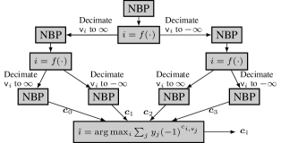
We start by running \acNBP for iterations. We then identify the \acVN with the lowest absolute a posteriori \acLLR , i.e., the least reliable \acLLR and decimate it to , i.e., set . Since the correct sign is unknown, we build a decoding tree: Each time we decimate a \acVN, we create two new graphs where in one the \acVN is decimated to and in the other the \acVN is decimated to . We then run the \acNBP decoder for each of the two graphs. We alternate between running \acNBP and decimation times. In Fig. 1, we depict the decoding tree for .
3.2 Learned Decimation Stage
While using the previously described list-based decimation allows to significantly boost the performance, it has the drawback that the complexity increases exponentially in the number of decimations. To reduce the size of the decoding tree, we propose an \acNN-based approach. More precisely, instead of continuing to unfold the decoding tree, we use an \acNN to decide to which value each \acVN should be decimated. The \acNN takes the incoming messages to the node and the channel \acLLR as input and outputs a value whose absolute value is then added to the channel message. The sign is kept according to the output \acLLR of the respective node. Hence, we decimate each \acVN according to
where denotes the \acNN and denotes all trainable parameters of the \acNN. The same \acNN is applied for all \acpVN and weights are shared between \acpVN and all decimation steps. We alternate learned decimation and running \acNBP times.
After the list-based decimations and learned decimations, we obtain codeword candidates and we choose the most likely codeword. The \acNBPD decoder is described in Algorithm 1.
3.3 Training
We perform training in two stages. We first consider a conventional \acNBP decoder with weights tied over the iterations. We train this decoder using the multiloss bitwise cross-entropy between the output \acpLLR of each \acVN layer and the correct codeword as the loss function and the Adam optimizer [2]. We then freeze the learned weights and unroll the \acNBPD() decoder. To reduce the complexity of the training procedure, we only consider the correct path through the decoding tree in the list-based decimation stage, i.e., we assume a genie that provides the correct sign of the decimated \acVN. This incurs no loss in \acBLER as, of the decoders, only the one with the correct decisions can return the correct codeword. We train the unrolled \acNBPD decoder using the multiloss bitwise cross-entropy between the output \acpLLR of each \acVN layer and the correct codeword as the loss function and the Adam optimizer.
3.4 Complexity Discussion
On a high level, by disregarding hardware implementation details, the \acCN update is the most complex operation due to the evaluation of the and inverse functions. A commonly used complexity measure is given by [19], where is the average \acCN degree and the number of \acpCN. The complexity of the \acNBPD decoder follows as
The memory requirement for the decoders is dominated by the number of weights that need to be stored. For the \acNBP decoder, this corresponds to the number of edges in the Tanner graph. In the case of \acNBPD, additionally the weights of the \acNN need to be taken into account. Note that the weights also entail additional multiplications.
4 Numerical Results
In this work, we consider an \acLDPC code of length and rate with average \acCN degree as defined by the CCSDS standard. Its parity-check matrix is of size . It is important to note that the presented concepts are not limited to a specific code and extend to any other sparse code.
For training the \acNBP and \acNBPD decoders, the batch size was set to , the learning rate to , and the Adam optimizer was used for gradient updates. The \acNN of the \acNBPD decoder consists of three layers where the first and second layer contain neurons and use the ReLU activation function, and the third layer consists of a single neuron with no activation function (i.e., a linear layer).
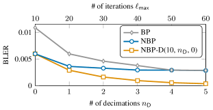
In Fig. 2, we plot the \acBLER as a function of the number of iterations for conventional \acBP, \acNBP, and \acNBPD for which , i.e., no learned decimation is employed. For a fixed number of iterations, \acNBP outperforms \acBP. For \acLDPC codes, the gain of \acNBP over \acBP appears to vanish with an increasing number of iterations, and at iterations \acBP and \acNBP have virtually the same performance. Importantly, increasing the number of iterations even further does not result in an improved performance. Considering the \acNBPD decoder, the decimation enables us to outperform (N)BP, even for a single decimation. It is important to note that while the complexity of (N)BP increases linearly in the number of iterations, the complexity of \acNBPD increases exponentially in the number of decimations .
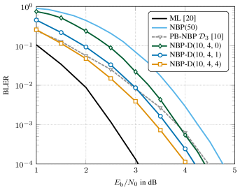
In Fig. 3, we show the \acBLER as a function of . \AcNBP with iterations () performs about from \acML. Increasing the number of iterations even further would not result in a better performance (see Fig. 2). improves by over and matches the performance of pruning-based NBP in [10]. Adding a single learned decimation () improves the performance by . Allowing four learned decimation steps (), the gap to \acML is further reduced to slightly less than . The choice of is a trade-off between performance and complexity. Increasing will eventually lead to \acML decoding. Relying solely on learned decimation () is not competitive as the correct choice of the sign for \acpVN of low reliability is never guaranteed. In Table 1, we compare the complexities for the decoders in Fig. 3. The numbers in parentheses indicate how much more complex a decoder is with reference to .
5 Conclusion
NBP,NBPD We proposed a \acNBPD decoder for \acLDPC codes. By combining a list-based decimation stage and a learned decimation stage where a neural network learns which \acpVN to decimate, we have shown that we can significantly improve the performance of \acBP and \acNBP, and achieve a performance within from \acML. The concept of \acNBPD can be applied to any other short block code. For sparse codes, similar performance improvements can be expected.
References
- [1] Eliya Nachmani, Yair Be’ery, and David Burshtein, “Learning to decode linear codes using deep learning,” in Proc. Annu. Allerton Conf. Commun., Control, Comput., Allerton, IL, USA, Sep. 2016, pp. 341–346.
- [2] Eliya Nachmani, Elad Marciano, Loren Lugosch, Warren J. Gross, David Burshtein, and Yair Be’ery, “Deep learning methods for improved decoding of linear codes,” IEEE J. Sel. Topics Signal Process., vol. 12, no. 1, pp. 119–131, Feb. 2018.
- [3] Jinghu Chen and Marc P. C. Fossorier, “Near optimum universal belief propagation based decoding of low-density parity check codes,” IEEE Trans. Commun., vol. 50, no. 3, pp. 406–414, Mar. 2002.
- [4] Martin Bossert and Ferdinand Hergert, “Hard- and soft-decision decoding beyond the half minimum distance—an algorithm for linear codes,” IEEE Trans. Inf. Theory, vol. 32, no. 5, pp. 709–714, Sep. 1986.
- [5] Aditi Kothiyal, Oscar Y. Takeshita, Wenyi Jin, and Marc Fossorier, “Iterative reliability-based decoding of linear block codes with adaptive belief propagation,” IEEE Commun. Lett., vol. 9, no. 12, pp. 1067–1069, Dec. 2005.
- [6] Jing Jiang and Krisha R. Narayanan, “Iterative soft-input soft-output decoding of Reed-Solomon codes by adapting the parity-check matrix,” IEEE Trans. Inf. Theory, vol. 52, no. 8, pp. 3746–3756, Aug. 2006.
- [7] Thomas R. Halford and Keith M. Chugg, “Random redundant soft-in soft-out decoding of linear block codes,” in Proc. IEEE Int. Symp. Inf. Theory (ISIT), Seattle, WA, USA, Jun. 2006, pp. 2230–2234.
- [8] Thorsten Hehn, Johannes Huber, Olgica Milenkovic, and Stefan Laendner, “Multiple-bases belief-propagation decoding of high-density cyclic codes,” IEEE Trans. Commun., vol. 58, no. 1, pp. 1–8, Jan. 2010.
- [9] Elia Santi, Christian Häger, and Henry D. Pfister, “Decoding Reed-Muller codes using minimum-weight parity checks,” in Proc. IEEE Int. Symp. Inf. Theory (ISIT), Vail, CO, USA, Jun. 2018, pp. 1296–1300.
- [10] Andreas Buchberger, Christian Häger, Henry Pfister, Laurent Schmalen, and Alexandre Graell i Amat, “Pruning neural belief propagation decoders,” in Proc. IEEE Int. Symp. Inf. Theory (ISIT), Los Angeles, CA, USA, Jun. 2020, pp. 338–342.
- [11] David Chase, “A class of algorithms for decoding block codes with channel measurement information,” IEEE Trans. Inf. Theory, vol. 18, no. 1, pp. 170–182, Jan. 1972.
- [12] H. Pishro-Nik and F. Fekri, “On decoding of low-density parity-check codes over the binary erasure channel,” IEEE Trans. Inf. Theory, vol. 50, no. 3, pp. 439–454, Mar. 2004.
- [13] Cyril Méasson, Andrea Montanari, and Rüdiger Urbanke, “Maxwell construction: The hidden bridge between iterative and maximum a posteriori decoding,” IEEE Trans. Inf. Theory, vol. 54, no. 12, pp. 5277–5307, Dec. 2008.
- [14] Tomáš Filler and Jessica Fridrich, “Binary quantization using belief propagation with decimation over factor graphs of LDGM codes,” in Proc. Annu. Allerton Conf. Commun., Control, Comput., Monticello, IL, USA, Sep. 2007.
- [15] Martin J. Wainwright, Elitza Maneva, and Emin Martinian, “Lossy source compression using low-density generator matrix codes: Analysis and algorithms,” IEEE Trans. Inf. Theory, vol. 56, no. 3, pp. 1351–1368, Mar. 2010.
- [16] Daniel Castanheira and Atilio Gameiro, “Lossy source coding using belief propagation and soft-decimation over LDGM codes,” in Proc.Int. Symp. Pers. Indoor Mobile Radio Commun. (PIMRC), Istanbul, Turkey, Sep. 2010, pp. 413–436.
- [17] Vahid Aref, Nicolas Macris, and Marc Vuffray, “Approaching the rate-distortion limit with spatial coupling, belief propagation, and decimation,” IEEE Trans. Inf. Theory, vol. 61, no. 7, pp. 3954–3979, Jul. 2015.
- [18] Mengke Lian, Fabrizio Carpi, Christian Häger, and Henry D. Pfister, “Learned belief-propagation decoding with simple scaling and SNR adaptation,” in Proc. IEEE Int. Symp. Inf. Theory (ISIT), Paris, France, Jul. 2019, pp. 161–165.
- [19] Benjamin Smith, Masoud Ardakani, Wei Yu, and Frank R. Kschischang, “Design of irregular LDPC codes with optimized performance-complexity tradeoff,” IEEE Trans. Commun., vol. 58, no. 2, pp. 489–499, Feb. 2010.
- [20] Michael Helmling, Stefan Scholl, Florian Gensheimer, Tobias Dietz, Kira Kraft, Stefan Ruzika, and Norbert Wehn, “Database of channel codes and ML simulation results,” www.uni-kl.de/channel-codes, 2019.