Capped norm linear discriminant analysis and its applications

Abstract

Classical linear discriminant analysis (LDA) is based on squared Frobenious norm and hence is sensitive to outliers and noise. To improve the robustness of LDA, in this paper, we introduce capped $l_{2,1}$-norm of a matrix, which employs non-squared $l_{2}$-norm and “capped” operation, and further propose a novel capped $l_{2,1}$-norm linear discriminant analysis, called CLDA. Due to the use of capped $l_{2,1}$-norm, CLDA can effectively remove extreme outliers and suppress the effect of noise data. In fact, CLDA can be also viewed as a weighted LDA. CLDA is solved through a series of generalized eigenvalue problems with theoretical convergency. The experimental results on an artificial data set, some UCI data sets and two image data sets demonstrate the effectiveness of CLDA.

I Introduction

The aim of dimensionality reduction is to embed high dimensional data into a low-dimensional space such that the most discriminative information is preserved. The projected data obtained by dimensionality reduction can be used in subsequent data mining tasks including classification, computer visualization, etc. In supervised learning, linear discriminant analysis (LDA) [1, 2] is one of the most useful and popular dimensionality reduction methods, and has been applied in many area, including multimodal dimensionality reduction [3], audiovisual speech recognition [4], image recognition [5, 6], clustering [7], and tensor extension [8, 9]. LDA aims to learn a set of optimal projections to extract useful discriminative information, through maximizing the between-class distance and simultaneously minimizing the within-class distance in the projected space.

However, the construction of LDA was based on squared Frobenious norm (F-norm), or squared $l_{2}$-norm in essence. When facing data with noise or outliers, LDA will be the sensitive to them, which may in turn lead the drifting of projections away from the desired directions. To alleviate this problem, many researchers tried to improve the robustness of LDA. For example, using subspace information [10, 11, 12, 13], considering robust counterparts of sample means and covariance matrices [14, 15, 16, 17], using data uncertainty and optimizing for the worst-case [18], incorporating data local information [19, 20, 21, 22]. As an effective robust replacement of squared $l_{2}$-norm, $l_{1}$-norm was usually used to resist outliers. By directly replacing $l_{2}$-norm with $l_{1}$-norm in LDA, several ratio form $l_{1}$-norm based LDA along with different solving algorithms and applications were studied [23, 24, 25, 26], for example, sum of $l_{1}$-norm based LDA [27], constraint $l_{1}$-norm based LDA [28, 29, 30], and error minimized $l_{1}$-norm based LDA [31, 32]. Some $l_{1}$-based methods were also extended to $l_{p}$-norm ones [33, 34, 35] or corresponding matrix input LDAs [36, 37, 38, 39].

Since $l_{1}$-norm was not rotational invariant [40], another robust and rotational invariant R₁-norm based LDA was studied in [41]. R₁-norm of a matrix was defined as an $l_{1}$-norm sum of vector $l_{2}$-norms. R₁-norm used the $l_{2}$-norm rather than squared $l_{2}$-norm as basic norm, and considered the $l_{1}$-norm sum, which largely reduced the importance of outliers, and therefore had robustness. R₁-norm was also known as $l_{2,1}$-norm in [42], and was generalized to $l_{p,q}$-norm for arbitrary $p,q>0$. $l_{2,1}$-norm based LDA was also studied [43]. However, though $l_{2,1}$-norm is robust, it still will suffer from the existence of odd points with extremely large norm. In this situation, even $l_{2,1}$-norm is not robust enough to reduce the effect of outliers. What if we can remove this influence or limit it within some boundary? In fact, this idea was employed in previous study to construct robust machine learning models, named capped norm. The central ideal of “capped” operation is to add an upper bound on common norms. For example, capped $l_{2}$-norm for robust feature learning [44], capped $l_{2,1}$-norm for regression and classification [45, 46], capped $l_{p}$-norm for classification [47], capped nuclear norm for matrix factorization or completion [48, 49], capped trace norm [50] for robust principal component analysis. We found that though most of the above methods seemed to use different capped norms, and were applied to different machine learning models, most of them were essentially of the form

$$\sum_{j=1}^{s}\min\{||\textbf{m}_{j}||_{2},\epsilon\},$$ (1)

where $\textbf{m}_{j}$, $j=1,2,\ldots,s$, was a series of column vectors and $\epsilon>0$. From (1), it can be seen that the capped operation can effectively remove outliers and noise beyond $\epsilon$ and benefit the input control. Therefore, $\epsilon$ is a thresholding parameter for picking out extreme data outliers. If we do not cap the data with extremely large norm, it will affect the recognition result dramatically.

In (1), if we deem $\textbf{m}_{j}$ as the $j$-th column of a matrix $\textbf{M}_{r\times s}$, $j=1,2,\ldots,s$, then we may define a “norm” for the matrix $\textbf{M}_{r\times s}$. This motivates us to give the definition of capped norm of a matrix. As shown above, the existing works either define a capped norm directly as a loss or apply the capped operation on elements or vectors. In fact, in [51], the authors defined a capped $l_{2,1}$-norm of a matrix. In this paper, we introduce a general capped norm of a matrix, named capped $l_{p,q}$-norm. In specific, given some $\epsilon>0$ and $p,q>0$, we formally define a capped $l_{p,q}$-norm of a matrix $\textbf{M}_{r\times s}$ as

$$\|\textbf{M}\|_{cap\,{p,q}}=\left(\sum_{j=1}^{s}\min\{||\textbf{m}_{j}||_{p}^{q},\epsilon\}\right)^{\frac{1}{q}},$$ (2)

where $p,q>0$. It should be noted that even we call them norms, capped $l_{2,1}$-norm and capped $l_{p,q}$-norm are not actual norms. In fact, as $T\ell_{1}$-norm [52], they do not satisfy homogeneity. However, when $p,q\geq 1$, it satisfies the positive scalability and triangle inequality. Clearly, $\|\textbf{M}\|_{cap\,{p,q}}\geq 0$ and it can be easily verified that

$$\|\textbf{A+B}\|_{cap\,{p,q}}\leq\|\textbf{A}\|_{cap\,{p,q}}+\|\textbf{B}\|_{cap\,{p,q}}.$$ (3)

However, as $Tl_{1}$-norm, it does not affect the robustness property, and we still call it a norm.

Considering the robustness of vector $l_{2}$-norm and $l_{1}$-norm, in this paper we only consider matrix capped $l_{2,1}$-norm, whose definition is based on vector $l_{2}$-norm and $l_{1}$-norm. Compared to Frobenius norm (F-norm) which is defined as $\|\textbf{M}\|_{F}=\sqrt{\sum_{j=1}^{s}\sum_{i=1}^{r}m_{ij}^{2}}=\sqrt{\sum_{j=1}^{s}||\textbf{m}_{j}||_{2}^{2}}$, squared F-norm, and $l_{2,1}$-norm which is defined as $\|\textbf{M}\|_{2,1}=\sum_{j=1}^{s}\sqrt{\sum_{i=1}^{r}m_{ij}^{2}}=\sum_{j=1}^{s}||\textbf{m}_{j}||_{2}$, capped $l_{2,1}$-norm can effectively suppress the effect of outliers and resist noise. The illustration of capped $l_{2,1}$-norm is demonstrated in Fig.1. In reality, while data outliers exist, feature noise can also exist. Suppose M is a data matrix with each column being a data sample. Since capped $l_{2,1}$-norm is summed over all “capped” data samples, it is robust to outliers. In addition, since capped $l_{2,1}$-norm adopts $l_{2}$-norm as a basic norm that acts on the $j$-th data sample $\textbf{m}_{j}$, it is also robust to feature noise.

Figure 1: Illustration of capped $l_{2,1}$-norm.

In this paper, based on the above defined capped $l_{2,1}$-norm, we propose a capped $l_{2,1}$-norm linear discriminant analysis (CLDA). Compared with classical LDA which utilized squared F-norm, the proposed CLDA is robust to outliers and noise. In specific, CLDA has following characteristics:

(i) A capped $l_{p,q}$-norm for arbitrary $p,q>0$ of a matrix is formally introduced, and a novel linear discriminant analysis based on capped $l_{2,1}$-norm named CLDA is proposed.

(ii) The capped $l_{2,1}$-norm used in CLDA makes it robust to data outliers and feature noise.

(iii) An effective algorithm is designed to solve the proposed non-smooth and non-convex optimization problem. The theoretical analysis of the proposed algorithm is also given.

(iv) Experimental results on an artificial data, some UCI data and two image data demonstrate the effectiveness of CLDA.

The paper is organized as follows. Section II briefly reviews LDA. Section III proposes CLDA and its corresponding analysis. Section IV makes comparisons of CLDA with its related approaches. Concluding remarks are given in Section V.

The notation of the paper is listed as follows. All vectors are column ones, and vectors and matrices are shown in bold. We consider the training data set $T=\{\textbf{x}_{1},\,\textbf{x}_{2},\ldots,\,\textbf{x}_{N}\}$ with associated class labels $y_{1},\,y_{2},\ldots,\,y_{N}$ belonging to $\{1,\,2,\,\ldots,c\}$, where $\textbf{x}_{l}\in\mathbb{R}^{n}$ for $l=1,\,2,\,\ldots,N$. Write $\textbf{X}=(\textbf{x}_{1},\,\textbf{x}_{2},\ldots,\,\textbf{x}_{N})\in\mathbb{R}^{n\times N}$ as the corresponding data matrix of $T$. Assume the $i$-th class contains $N_{i}$ samples, $i=1,2,\ldots,c$. Then $\sum\limits_{i=1}^{c}N_{i}=N$. Let $\overline{\textbf{x}}=\frac{1}{N}\sum\limits_{l=1}^{N}\textbf{x}_{l}$ be the mean of all samples and ${\overline{\textbf{x}}}_{i}=\frac{1}{N_{i}}\sum\limits_{j=1}^{N_{i}}\textbf{x}_{i}^{j}$ be the mean of samples in the $i$-th class, where $\textbf{x}_{i}^{j}$ is the $j$-th sample in the $i$-th class, $i=1,2,\ldots,c$, $j=1,2,\ldots,N_{i}$. For simplicity, we write $\|\cdot\|_{2}$ as $\|\cdot\|$.

II Linear discriminant analysis

LDA performs dimensionality reduction by seeking a linear transformation matrix $\textbf{W}\in\mathbb{R}^{n\times d}$, $d\leq n$ such that the between-class scatter distance is maximized and meanwhile the within-class scatter distance is minimized in the projected space. In specific, LDA formulates as

$$\begin{split}\underset{\textbf{W}}{\max}~{}~{}&\frac{\sum\limits_{i=1}^{c}N_{i}\|\textbf{W}^{T}(\overline{\textbf{x}}_{i}-\overline{\textbf{x}})\|^{2}}{\sum\limits_{i=1}^{c}\sum\limits_{j=1}^{N_{i}}\|\textbf{W}^{T}(\textbf{x}_{i}^{j}-\overline{\textbf{x}}_{i})\|^{2}}.\\ \end{split}$$ (4)

Write

$$\textbf{H}_{b}=(\sqrt{N_{1}}(\overline{\textbf{x}}_{1}-\overline{\textbf{x}}),\sqrt{N_{2}}(\overline{\textbf{x}}_{2}-\overline{\textbf{x}}),\cdots,\sqrt{N_{c}}(\overline{\textbf{x}}_{c}-\overline{\textbf{x}}))\in\mathbb{R}^{n\times c}$$ (5)

and

$$\textbf{H}_{w}=((\textbf{x}_{1}^{1}-\overline{\textbf{x}}_{1}),\cdots,(\textbf{x}_{1}^{N_{1}}-\overline{\textbf{x}}_{1}),\cdots,(\textbf{x}_{c}^{1}-\overline{\textbf{x}}_{c}),\cdots,(\textbf{x}_{c}^{N_{c}}-\overline{\textbf{x}}_{c}))\in\mathbb{R}^{n\times N},$$ (6)

then (4) is equivalent to

$$\underset{\textbf{W}}{\max}~{}~{}\frac{\|\textbf{W}^{T}\textbf{H}_{b}\|_{F}^{2}}{\|\textbf{W}^{T}\textbf{H}_{w}\|_{F}^{2}}.$$ (7)

The optimal solution $\textbf{W}=(\textbf{w}_{1},\ldots,\textbf{w}_{d})\in\mathbb{R}^{n\times d}$ of (4) can be obtained from a generalized problem $\textbf{S}_{b}\textbf{w}=\lambda\textbf{S}_{w}\textbf{w}$ with $\lambda\not=0$, where $\textbf{S}_{b}$ and $\textbf{S}_{w}$ are between-class scatter matrix and within-class scatter matrix defined by

$$\textbf{S}_{b}=\frac{1}{N}\textbf{H}_{b}\textbf{H}_{b}^{T}$$ (8)

and

$$\textbf{S}_{w}=\frac{1}{N}\textbf{H}_{w}\textbf{H}_{w}^{T}$$ (9)

respectively. If $\textbf{S}_{w}$ is nonsingular, then W is given by the first $d$ largest eigenvalues of $(\textbf{S}_{w})^{-1}\textbf{S}_{b}$.

III The proposed capped $l_{2,1}$-norm linear discriminant analysis

III-A Problem formulation

As we see, in LDA, the within-class distance and between-class distance are based on squared F-norm, which makes LDA sensitive to outliers and noise. The squared operation on $F$-norm or $l_{2}$-norm metric will enlarge the effect of outliers and noise. If we discard the square operation and consider just F-norm or $l_{2}$-norm, the robustness will be improved [53]. However, even F-norm or $l_{2}$-norm may lose control to some outliers with large norms. In this situation, it is necessary to set a bar to remove outliers. This motivates us to introduce the aforementioned capped $l_{2,1}$-norm into LDA and construct a novel capped $l_{2,1}$-norm based LDA (CLDA). In specific, the proposed CLDA has the following optimization problem

$$\underset{\textbf{W}}{\min}~{}~{}\frac{\|\textbf{W}^{T}\textbf{H}_{w}\|_{cap\,{2,1}}}{\|\textbf{W}^{T}\textbf{H}_{b}\|_{cap\,{2,1}}}=\frac{\sum\limits_{i=1}^{c}\sum\limits_{j=1}^{N_{i}}\min\left(\|\textbf{W}^{T}(\textbf{x}_{i}^{j}-\overline{\textbf{x}}_{i})\|,\epsilon\right)}{\sum\limits_{i=1}^{c}\min\left(\|\sqrt{N_{i}}\textbf{W}^{T}(\overline{\textbf{x}}_{i}-\overline{\textbf{x}})\|,\epsilon\right)},$$ (10)

where $\epsilon>0$ is a thresholding parameter. It can be seen that both the within-class distance and between-class distance are measured by capped $l_{2,1}$-norm. In these two capped $l_{2,1}$-norm terms, the application of $l_{2}$-norm on projected data $\textbf{W}^{T}(\textbf{x}_{i}^{j}-\overline{\textbf{x}}_{i})$ and $\sqrt{N_{i}}\textbf{W}^{T}(\overline{\textbf{x}}_{i}-\overline{\textbf{x}})$ reduces the negative influence of noise and outliers, and the $l_{1}$-norm sum over the “capped” projected data restricted by parameter $\epsilon$ removes the effect of extreme data outliers. To solve (10), we first recast it to an equivalent form

$$\begin{split}\underset{\textbf{W}}{\min}&~{}~{}{\sum\limits_{i=1}^{c}\sum\limits_{j=1}^{N_{i}}\min(\|\textbf{W}^{T}(\textbf{x}_{i}^{j}-\overline{\textbf{x}}_{i})\|,\epsilon)}\\ \hbox{s.t.\ }&{\sum\limits_{i=1}^{c}\min(\|\sqrt{N_{i}}\textbf{W}^{T}(\overline{\textbf{x}}_{i}-\overline{\textbf{x}})\|,\epsilon)}=1.\end{split}$$ (11)

The above formulation of CLDA in fact can be viewed as a formally generalized eigenvalue optimization problem. Define $F_{ij}=\|\textbf{W}^{T}(\textbf{x}_{i}^{j}-\overline{\textbf{x}}_{i})\|^{-1}\cdot Ind(\|\textbf{W}^{T}(\textbf{x}_{i}^{j}-\overline{\textbf{x}}_{i})\|\leq\epsilon)$, where $Ind(\cdot)$ is the indicator function satisfying $Ind(\|\textbf{W}^{T}(\textbf{x}_{i}^{j}-\overline{\textbf{x}}_{i})\|\leq\epsilon)=1$ if $\|\textbf{W}^{T}(\textbf{x}_{i}^{j}-\overline{\textbf{x}}_{i})\|\leq\epsilon$, and 0 otherwise, and define $\textbf{F}\in\mathbb{R}^{N\times N}$ as the diagonal matrix with its diagonal element $F_{ij}$, $i=1,2,\ldots,c,~{},j=1,2,\ldots,N_{i}$. Then

$$\begin{split}&\underset{\textbf{W}}{\min}~{}~{}\sum\limits_{i=1}^{c}\sum\limits_{j=1}^{N_{i}}\min(\|\textbf{W}^{T}(\textbf{x}_{i}^{j}-\overline{\textbf{x}}_{i})\|,\epsilon)\\ =~{}&\underset{\textbf{W}}{\min}~{}~{}\sum\limits_{i=1}^{c}\sum\limits_{j=1}^{N_{i}}F_{ij}\|\textbf{W}^{T}(\textbf{x}_{i}^{j}-\overline{\textbf{x}}_{i})\|^{2}\\ =~{}&\underset{\textbf{W}}{\min}~{}~{}\hbox{tr}(\textbf{W}^{T}\textbf{H}_{w}\textbf{F}\textbf{H}_{w}^{T}\textbf{W})\\ =~{}&\underset{\textbf{W}}{\min}~{}~{}\hbox{tr}(\textbf{W}^{T}\textbf{S}_{1}\textbf{W}),\end{split}$$ (12)

where $\textbf{S}_{1}=\textbf{H}_{w}\textbf{F}\textbf{H}_{w}^{T}$.

Similarly, denote $G_{i}=\|\sqrt{N_{i}}\textbf{W}^{T}(\overline{\textbf{x}}_{i}-\overline{\textbf{x}})\|^{-1}\cdot Ind(\sqrt{N_{i}}\|\textbf{W}^{T}(\overline{\textbf{x}}_{i}-\overline{\textbf{x}})\|\leq\epsilon)$ and $\textbf{G}\in\mathbb{R}^{c\times c}$ as the diagonal matrix with its $(i,i)$-th element $G_{i}$. Then the left side of constraint of (11) is equivalent to

$$\sum\limits_{i=1}^{c}G_{i}\|\sqrt{N_{i}}\textbf{W}^{T}(\overline{\textbf{x}}_{i}-\overline{\textbf{x}})\|^{2}=\hbox{tr}(\textbf{W}^{T}\textbf{S}_{2}\textbf{W}),$$ (13)

where $\textbf{S}_{2}=\textbf{H}_{b}\textbf{G}\textbf{H}_{b}^{T}$. Therefore, CLDA (11) can be recast as

$$\begin{split}\underset{\textbf{W}}{\min}~{}&\hbox{tr}(\textbf{W}^{T}\textbf{S}_{1}\textbf{W})\\ \hbox{s.t.~{}~{}}\hbox{tr}&(\textbf{W}^{T}\textbf{S}_{2}\textbf{W})=\Delta,\end{split}$$ (14)

where $\Delta$ is some constant. By observing (14), we may deem CLDA as a generalized eigenvalue optimization problem in form, since $\textbf{S}_{1}$ and $\textbf{S}_{2}$ are both related to W. We call $\textbf{S}_{1}$ as within-class scatter and $\textbf{S}_{2}$ as between-class scatter of CLDA.

It should be noted that the within-class scatter $\textbf{S}_{1}$ and between-class scatter $\textbf{S}_{2}$ in CLDA are in fact weighted $\textbf{S}_{w}$ and $\textbf{S}_{b}$ in LDA, and F and G are their corresponding weighting matrices. These weights make CLDA robust to outliers and noise. On one hand, non-squared $l_{2}$-norm brings robustness to feature noise. One the other hand, for projected data that have norm larger than $\epsilon$ will be ignored since the corresponding weight is 0, and these data are considered as outliers. For projected data having large norms but less than $\epsilon$, small weights are given to these data, and these data may be noise data. Therefore, CLDA is robust to outliers and noise.

III-B The solving algorithm of CLDA and convergence analysis

In the following, we solve (14). For fixed $\textbf{S}_{1}$ and $\textbf{S}_{2}$, (14) is a generalized eigenvalue problem. Clearly, $\textbf{S}_{1}$ and $\textbf{S}_{2}$ depend on F and G respectively, and hence depend on W. Therefore, to solve this problem, we employ an iterative technique. In specific, we first initialize $\textbf{W}^{(0)}$ as the first $d$ columns of the identity $\textbf{I}\in\mathbb{R}^{n\times n}$. Then in the $t$-th iteration, $\textbf{S}_{1}^{(t)}$ and $\textbf{S}_{2}^{(t)}$ are computed according to

$$\begin{split}\textbf{S}_{1}^{(t)}&=\textbf{H}_{w}\textbf{F}^{(t)}\textbf{H}_{w}^{T}\\ \textbf{S}_{2}^{(t)}&=\textbf{H}_{b}\textbf{G}^{(t)}\textbf{H}_{b}^{T},\end{split}$$ (15)

where the diagonal elements of $\textbf{F}^{(t)}$ and $\textbf{G}^{(t)}$ are given by

$$F_{ij}^{(t)}=\|(\textbf{W}^{(t)})^{T}(\textbf{x}_{i}^{j}-\overline{\textbf{x}}_{i})\|^{-1}\cdot Ind(\|(\textbf{W}^{(t)})^{T}(\textbf{x}_{i}^{j}-\overline{\textbf{x}}_{i})\|\leq\epsilon)$$

and

$$G_{i}^{(t)}=\|\sqrt{N_{i}}(\textbf{W}^{(t)})^{T}(\overline{\textbf{x}}_{i}-\overline{\textbf{x}})\|^{-1}\cdot Ind(\|\sqrt{N_{i}}(\textbf{W}^{(t)})^{T}(\overline{\textbf{x}}_{i}-\overline{\textbf{x}})\|\leq\epsilon).$$

After obtaining $\textbf{S}_{1}^{(t)}$ and $\textbf{S}_{2}^{(t)}$, the optimal solution $\textbf{W}^{(t+1)}$ of (14) is computed by solving the following problem

$$\begin{split}\textbf{W}^{(t+1)}&=\underset{\textbf{W}}{\arg\min}~{}~{}\hbox{tr}(\textbf{W}^{T}\textbf{S}_{1}^{(t)}\textbf{W})\\ &\hbox{s.t.\ }{\hbox{tr}(\textbf{W}^{T}\textbf{S}_{2}^{(t)}\textbf{W})}=\Delta.\end{split}$$ (16)

The optimal solution $\textbf{W}^{(t+1)}$ of (16) can be given by the first $d$ eigenvectors corresponding to first $d$ smallest nonzero eigenvalues of the generalized eigenvalue problem $\textbf{S}_{1}^{(t)}\textbf{w}=\lambda\textbf{S}_{2}^{(t)}\textbf{w}$, where $\lambda$ is its eigenvalue. After reaching maximum iteration number or convergence, the optimal $\textbf{W}^{*}$ is set to $\textbf{W}^{(t+1)}$. After obtaining $\textbf{W}^{*}$, for a new coming sample $\textbf{x}\in\mathbb{R}^{n}$, its representation in low dimension space is $\widehat{\textbf{x}}=(\textbf{W}^{*})^{T}\textbf{x}$.

The solving procedure is summarized in Algorithm 1.

$\mathbf{Algorithm~{}1.}$  CLDA solving Algorithm

Input: Training data set $T=\{\textbf{x}_{1},\,\textbf{x}_{2},\ldots,\,\textbf{x}_{N}\}$, reduced

dimension $d\leq n$, maximum iteration number $Itmax$, and

parameter $\epsilon>0$.

Process:

1. Initialize $\textbf{W}^{(0)}$ as the first $d$ columns of the identity

matrix $\textbf{I}\in\mathbb{R}^{n\times n}$;

2. For $t=0,1,2,\ldots$, repeat

Compute $\textbf{S}_{1}^{(t)}$ and $\textbf{S}_{2}^{(t)}$ by (15);

Compute $\textbf{W}^{(t+1)}$ by solving (16);

Set $t=t+1$;

Until reaching maximum iteration number $Itmax$ or

convergence.

Output: $\textbf{W}^{*}=\textbf{W}^{(t+1)}$ and $\widehat{\textbf{x}}=(\textbf{W}^{*})^{T}\textbf{x}$.

We have the following convergency result about Algorithm 1.

Proposition 1.

The procedures of CLDA shown in Algorithm 1 monotonically decrease the objective of (11) in each step and converge to a local optimum.

Proof: Let $K^{(t)}$ be the index set of $i=1,2,\ldots,c,~{}j=1,2,\ldots,N_{i}$ that satisfies $\|(\textbf{W}^{(t)})^{T}(\textbf{x}_{i}^{j}-\overline{\textbf{x}}_{i})\|\leq\epsilon$, that is $K^{(t)}=\{(i,j):\|(\textbf{W}^{(t)})^{T}(\textbf{x}_{i}^{j}-\overline{\textbf{x}}_{i})\|\leq\epsilon\}$, $t=0,1,2,\ldots$. Denote $|K^{(t)}|$ as the number of elements in $K^{(t)}$. Since $\textbf{W}^{(t+1)}$ minimizes (16),

$$\begin{split}&\sum\limits_{(i,j)\in K^{(t)}}F_{ij}^{(t)}\|(\textbf{W}^{(t+1)})^{T}(\textbf{x}_{i}^{j}-\overline{\textbf{x}}_{i})\|^{2}\\ \leq&\sum\limits_{(i,j)\in K^{(t)}}F_{ij}^{(t)}\|(\textbf{W}^{(t)})^{T}(\textbf{x}_{i}^{j}-\overline{\textbf{x}}_{i})\|^{2}.\end{split}$$ (17)

On one hand, note that when $(i,j)\in K^{(t)}$, $F_{ij}^{(t)}=\|\textbf{W}^{T}(\textbf{x}_{i}^{j}-\overline{\textbf{x}}_{i})\|^{-1}$, we have

$$\begin{split}&\sum\limits_{(i,j)\in K^{(t)}}\frac{\|(\textbf{W}^{(t+1)})^{T}(\textbf{x}_{i}^{j}-\overline{\textbf{x}}_{i})\|^{2}}{2\|(\textbf{W}^{(t)})^{T}(\textbf{x}_{i}^{j}-\overline{\textbf{x}}_{i})\|}\\ \leq&\sum\limits_{(i,j)\in K^{(t)}}\frac{\|(\textbf{W}^{(t)})^{T}(\textbf{x}_{i}^{j}-\overline{\textbf{x}}_{i})\|^{2}}{2\|(\textbf{W}^{(t)})^{T}(\textbf{x}_{i}^{j}-\overline{\textbf{x}}_{i})\|}.\end{split}$$ (18)

From the inequality $\sqrt{a}-\frac{a}{2\sqrt{b}}\leq\sqrt{b}-\frac{b}{2\sqrt{b}}$ for arbitrary $a,b>0$, we have

$$\begin{split}&\sum\limits_{(i,j)\in K^{(t)}}\left({\|(\textbf{W}^{(t+1)})^{T}(\textbf{x}_{i}^{j}-\overline{\textbf{x}}_{i})\|}-\frac{\|(\textbf{W}^{(t+1)})^{T}(\textbf{x}_{i}^{j}-\overline{\textbf{x}}_{i})\|^{2}}{2\|(\textbf{W}^{(t)})^{T}(\textbf{x}_{i}^{j}-\overline{\textbf{x}}_{i})\|}\right)\\ \leq&\sum\limits_{(i,j)\in K^{(t)}}\left({\|(\textbf{W}^{(t)})^{T}(\textbf{x}_{i}^{j}-\overline{\textbf{x}}_{i})\|}-\frac{\|(\textbf{W}^{(t)})^{T}(\textbf{x}_{i}^{j}-\overline{\textbf{x}}_{i})\|^{2}}{2\|(\textbf{W}^{(t)})^{T}(\textbf{x}_{i}^{j}-\overline{\textbf{x}}_{i})\|}\right)\\ \end{split}$$ (19)

By adding (18) and (19) together, we obtain

$$\begin{split}\sum\limits_{(i,j)\in K^{(t)}}{\|(\textbf{W}^{(t+1)})^{T}(\textbf{x}_{i}^{j}-\overline{\textbf{x}}_{i})\|}\leq\sum\limits_{(i,j)\in K^{(t)}}{\|(\textbf{W}^{(t)})^{T}(\textbf{x}_{i}^{j}-\overline{\textbf{x}}_{i})\|}.\end{split}$$ (20)

Now adding term $(N-|K^{(t)}|)\epsilon$ to both sides of the above inequality, it follows

$$\begin{split}&\sum\limits_{(i,j)\in K^{(t)}}{\|(\textbf{W}^{(t+1)})^{T}(\textbf{x}_{i}^{j}-\overline{\textbf{x}}_{i})\|}+(N-|K^{(t)}|)\epsilon\\ \leq&\sum\limits_{(i,j)\in K^{(t)}}{\|(\textbf{W}^{(t)})^{T}(\textbf{x}_{i}^{j}-\overline{\textbf{x}}_{i})\|}+(N-K^{(t)}|)\epsilon.\end{split}$$ (21)

On the other hand, since $K^{(t+1)}=\{(i,j):\|(\textbf{W}^{(t+1)})^{T}(\textbf{x}_{i}^{j}-\overline{\textbf{x}}_{i})\|\leq\epsilon\}$, it can be verified that

$$\begin{split}&\sum\limits_{(i,j)\in K^{(t+1)}}{\|(\textbf{W}^{(t+1)})^{T}(\textbf{x}_{i}^{j}-\overline{\textbf{x}}_{i})\|}+(N-|K^{(t+1)}|)\epsilon\\ \leq&\sum\limits_{(i,j)\in K^{(r)}}{\|(\textbf{W}^{(t+1)})^{T}(\textbf{x}_{i}^{j}-\overline{\textbf{x}}_{i})\|}+(N-|K^{(r)}|)\epsilon\end{split}$$ (22)

for arbitrary $r=1,2,\ldots,t$. In fact, if $K^{(r)}=\emptyset$, (22) is obvious true from the definition of $K^{(t+1)}$. If $K^{(r)}\not=\emptyset$, we first write $K^{(r)}=K^{(r^{\prime})}\bigcup(K^{(r)}\backslash K^{(r^{\prime})})$, where $K^{(r^{\prime})}\subseteq K^{(t+1)}$. Then for $(i,j)\in K^{(r)}\backslash K^{(r^{\prime})}$, $\|(\textbf{W}^{(t+1)})^{T}(\textbf{x}_{i}^{j}-\overline{\textbf{x}}_{i})\|\geq\epsilon$. Therefore,

$$\begin{split}&\sum\limits_{(i,j)\in K^{(r)}}{\|(\textbf{W}^{(t+1)})^{T}(\textbf{x}_{i}^{j}-\overline{\textbf{x}}_{i})\|}+(N-|K^{(r)}|)\epsilon\\ =&\sum\limits_{(i,j)\in K^{(r^{\prime})}}{\|(\textbf{W}^{(t+1)})^{T}(\textbf{x}_{i}^{j}-\overline{\textbf{x}}_{i})\|}\\ &+\sum\limits_{(i,j)\in K^{(r)}\backslash K^{(r^{\prime})}}{\|(\textbf{W}^{(t+1)})^{T}(\textbf{x}_{i}^{j}-\overline{\textbf{x}}_{i})\|}+(N-|K^{(r)}|)\epsilon\\ \geq&\sum\limits_{(i,j)\in K^{(r^{\prime})}}{\|(\textbf{W}^{(t+1)})^{T}(\textbf{x}_{i}^{j}-\overline{\textbf{x}}_{i})\|}+(|K^{(r)}|-|K^{(r)}\cap K^{(r^{\prime})}|)\epsilon\\ &+(N-|K^{(r)}|)\epsilon\\ \geq&\sum\limits_{(i,j)\in K^{(r^{\prime})}}{\|(\textbf{W}^{(t+1)})^{T}(\textbf{x}_{i}^{j}-\overline{\textbf{x}}_{i})\|}+(N-|K^{(r^{\prime})}|)\epsilon\\ \geq&\sum\limits_{(i,j)\in K^{(t+1)}}{\|(\textbf{W}^{(t+1)})^{T}(\textbf{x}_{i}^{j}-\overline{\textbf{x}}_{i})\|}+(N-|K^{(t+1)}|)\epsilon.\end{split}$$ (23)

The last inequality of (23) follows from the fact that

$$\begin{split}&\sum\limits_{(i,j)\in K^{(t+1)}}{\|(\textbf{W}^{(t+1)})^{T}(\textbf{x}_{i}^{j}-\overline{\textbf{x}}_{i})\|}+(N-|K^{(t+1)}|)\epsilon\\ =&\sum\limits_{(i,j)\in K^{(r^{\prime})}}{\|(\textbf{W}^{(r^{\prime})})^{T}(\textbf{x}_{i}^{j}-\overline{\textbf{x}}_{i})\|}\\ &+\sum\limits_{(i,j)\in{K^{(t+1)}}\backslash K^{(r^{\prime})}}{\|(\textbf{W}^{(t+1)})^{T}(\textbf{x}_{i}^{j}-\overline{\textbf{x}}_{i})\|}+(N-|K^{(t+1)}|)\epsilon\\ \leq&\sum\limits_{(i,j)\in K^{(r^{\prime})}}{\|(\textbf{W}^{(r^{\prime})})^{T}(\textbf{x}_{i}^{j}-\overline{\textbf{x}}_{i})\|}+(|K^{(t+1)}|-|K^{(r^{\prime})}|)\epsilon\\ &+(N-|K^{(t+1)}|)\epsilon\\ =&\sum\limits_{(i,j)\in K^{(r^{\prime})}}{\|(\textbf{W}^{(r^{\prime})})^{T}(\textbf{x}_{i}^{j}-\overline{\textbf{x}}_{i})\|}+(N-|K^{(r^{\prime})}|)\epsilon\end{split}$$ (24)

In addition, (23) is clearly true for $K^{(r^{\prime})}=\emptyset$ and $K^{(r^{\prime})}=K^{(r)}$. Therefore, (22) holds. Taking $r=t$ in (22), and combing (21), it follows

$$\begin{split}&\sum\limits_{(i,j)\in K^{(t+1)}}{\|(\textbf{W}^{(t+1)})^{T}(\textbf{x}_{i}^{j}-\overline{\textbf{x}}_{i})\|}+(N-|K^{(t+1)}|)\epsilon\\ \leq&\sum\limits_{(i,j)\in K^{(t)}}{\|(\textbf{W}^{(t)})^{T}(\textbf{x}_{i}^{j}-\overline{\textbf{x}}_{i})\|}+(N-K^{(t)}|)\epsilon,\end{split}$$ (25)

which is just

$$\begin{split}&\sum\limits_{i=1}^{c}\sum\limits_{j=1}^{N_{i}}\min(\|(\textbf{W}^{(t+1)})^{T}(\textbf{x}_{i}^{j}-\overline{\textbf{x}}_{i})\|,\epsilon)\\ \leq&\sum\limits_{i=1}^{c}\sum\limits_{j=1}^{N_{i}}\min(\|(\textbf{W}^{(t+1)})^{T}(\textbf{x}_{i}^{j}-\overline{\textbf{x}}_{i})\|,\epsilon).\end{split}$$ (26)

Therefore, Algorithm 1 monotonically decreases the objective of (11) in each step. Since the objective of (11) is obviously lower bounded by 0, this completes the proof. $\square$

IV Experiments

In this section, we evaluate the performance of the proposed CLDA compared with its related methods, including LDA [1, 2], RDA [15], RLDA [29], LDA-L1 [23, 24], and L2BLDA [32]. The regularization parameter for RDA is selected from the set $\{10^{-5},10^{-4},\ldots,10^{-1},1,10\}$, $\rho$ for RLDA is selected from $\{0.1,0.5,1,5,50,100,1000\}$, the learning rate parameter for LDA-L1 is chosen from $\{10^{-6},10^{-5},\ldots,10^{2}\}$. All methods are carried out on a laptop with Intel i5 processor (2.60 GHz) with 4 GB RAM memory using MATLAB 2017a. Experiments are conducted on an artificial data set, some benchmark UCI data sets and two image data sets. Test classification accuracy ($\%$) is used to compare performance, which is obtained by applying nearest neighbor classifier on the projected test data after training dimensionality reduction methods.

IV-A An artificial data set

We first consider a two-class two-dimensional artificial data set, and project it to a one-dimensional space. Class 1 of the data is generated from a uniform distribution that horizontally distributed with 120 samples, and Class 2 is generated from a uniform distribution that vertically distributed with 120 samples. 50% samples of each class are randomly selected for training, and the rest ones are used for testing. To test the robustness of the proposed method, we add three extra outliers for each class, as shown in Fig.2(a). Test data are shown in Fig.2(b).

(a) Training data and projection directions

(b) Test data and projection directions

Figure 2: Training and test artificial data and projection directions obtained by all methods.

We apply all methods to the above polluted training data, and use the obtained projection directions to project both training data and test data to one-dimensional space. The classification results on projected test data are shown in Table I, which demonstrates that L2BLDA and our CLDA can separate two classes well. To see the results more clearly, we also show the obtained projection directions. From the construction of the data, we see the ideal projection direction is parallel to $x$-axis. We plot the projection direction of each method in Fig.2. From the figure, we see the proposed CLDA obtains projection direction that is very close to the ideal one, while other methods have deviation more or less. By further observing the projection data obtained by each method in Fig.3, it can be seen that except L2BLDA and our CLDA, other methods will misclassify samples.

TABLE I: Classification results on artificial test data.

Method	LDA	RDA	RLDA	LDA-L1	L2BLDA	CLDA
Accuracy	95.00	95.00	95.00	95.83	100.00	100.00

(a) LDA

(b) RDA

(c) RLDA

(d) LDAL1

(e) L2BLDA

(f) CLDA

Figure 3: Training and test artificial data and projection directions obtained by all methods.

IV-B Benchmark UCI data sets

TABLE II: UCI data sets information.

Data set	Sample no.	Feature no.	Class no.
Australian	690	14	2
BUPA	345	6	2
Car	1782	6	4
Credit	690	15	2
Diabetics	768	8	2
Echo	131	10	2
WPBC	198	34	2
German	1000	20	2
Haberman	306	3	2
Waveform	5000	21	2
House$\_$votes	435	16	2
Iris	150	4	3
Monks3	432	6	2
Sonar	208	60	2
Spect	267	44	2
CMC	1473	9	2
Dermatology	366	34	6
Glass	214	9	6
Heartc	303	14	2
Ionosphere	351	34	2
Seeds	300	2	2

In this subsection, the proposed CLDA and its compared methods are applied on 21 benchmark data sets, whose information is listed in Table II. In our experiment, all data are normalized to $[0,1]$. 10-fold cross validation is used for searching optimal parameter, and 10-time average test classification accuracy is adopted. Classification accuracies along with standard deviations for all methods are listed in Table III. “Acc” is short for accuracy ($\%$), and “Std” is short for standard deviation. By observing the results in Table III, we see that the proposed CLDA outperforms other methods on most of the data sets. On other data sets, CLDA performs comparable to the one with highest accuracy for most cases. To clearly see the superiority of CLDA, we compute the rank of each methods, as shown in Table IV. It can be seen that on most data sets CLDA has the highest rank, and on most other data sets its rank is also on the front. This leads to its highest average rank over all data sets.

TABLE III: Classification results on original UCI data sets.

Data set	LDA	RDA	RLDA	LDA-L1	L2BLDA	CLDA
	Acc$\pm$Std	Acc$\pm$Std	Acc$\pm$Std	Acc$\pm$Std	Acc$\pm$Std	Acc$\pm$Std
Australian	82.14 $\pm$ 4.62	81.95 $\pm$ 4.85	83.74 $\pm$ 4.02	83.76 $\pm$ 3.31	83.76 $\pm$ 3.31	82.02 $\pm$ 5.46
BUPA	57.66 $\pm$ 4.53	56.21 $\pm$ 8.73	66.03 $\pm$ 7.30	67.39 $\pm$ 4.13	67.39 $\pm$ 4.13	69.13 $\pm$ 5.99
Car	84.21 $\pm$ 4.84	84.86 $\pm$ 4.28	85.91 $\pm$ 7.85	94.34 $\pm$ 6.14	95.43 $\pm$ 2.69	94.04 $\pm$ 4.17
Credit	81.46 $\pm$ 4.02	81.15 $\pm$ 4.94	83.44 $\pm$ 4.02	83.69 $\pm$ 4.84	83.69 $\pm$ 4.84	83.30 $\pm$ 4.03
Diabetics	67.35 $\pm$ 4.61	70.18 $\pm$ 4.15	73.38 $\pm$ 3.53	71.31 $\pm$ 4.30	76.67 $\pm$ 3.79	73.80 $\pm$ 5.64
Echo	89.34 $\pm$ 8.97	87.19 $\pm$ 10.56	87.56 $\pm$ 12.18	91.59 $\pm$ 8.47	91.59 $\pm$ 8.47	97.02 $\pm$ 3.86
WPBC	78.39 $\pm$ 8.17	76.53 $\pm$ 13.88	82.57 $\pm$ 8.09	80.95 $\pm$ 7.08	80.95 $\pm$ 7.08	81.55 $\pm$ 9.49
German	67.50 $\pm$ 3.69	68.60 $\pm$ 3.66	72.90 $\pm$ 2.60	73.80 $\pm$ 4.21	75.80 $\pm$ 2.66	75.40 $\pm$ 3.95
Haberman	63.87 $\pm$ 11.70	67.46 $\pm$ 9.16	62.18 $\pm$ 10.46	67.53 $\pm$ 5.03	67.53 $\pm$ 5.03	69.94 $\pm$ 6.75
Waveform	79.99 $\pm$ 1.45	80.23 $\pm$ 1.78	80.93 $\pm$ 2.19	87.12 $\pm$ 1.18	87.12 $\pm$ 1.18	83.94 $\pm$ 1.62
House$\_$votes	93.10 $\pm$ 1.87	93.60 $\pm$ 3.00	94.50 $\pm$ 3.62	95.38 $\pm$ 2.68	95.38 $\pm$ 2.68	95.19 $\pm$ 2.26
Iris	96.00 $\pm$ 3.44	96.00 $\pm$ 3.44	94.67 $\pm$ 6.89	96.67 $\pm$ 5.67	94.00 $\pm$ 4.92	96.67 $\pm$ 4.71
Monks3	69.21 $\pm$ 13.83	61.34 $\pm$ 10.95	68.88 $\pm$ 4.84	70.34 $\pm$ 8.82	70.34 $\pm$ 8.82	84.02 $\pm$ 12.53
Sonar	71.69 $\pm$ 12.08	73.63 $\pm$ 10.29	89.51 $\pm$ 8.36	89.54 $\pm$ 6.79	90.82 $\pm$ 5.64	91.90 $\pm$ 5.52
Spect	72.89 $\pm$ 9.25	69.32 $\pm$ 9.45	81.95 $\pm$ 6.45	84.84 $\pm$ 6.09	84.84 $\pm$ 6.09	88.01 $\pm$ 5.56
CMC	68.91 $\pm$ 3.66	72.85 $\pm$ 2.26	69.17 $\pm$ 3.43	70.60 $\pm$ 2.17	72.93 $\pm$ 2.00	74.51 $\pm$ 2.49
Dermatology	97.26 $\pm$ 2.60	96.99 $\pm$ 3.03	96.49 $\pm$ 2.84	97.51 $\pm$ 3.08	94.44 $\pm$ 4.14	97.83 $\pm$ 1.74
Glass	64.68 $\pm$ 11.64	71.84 $\pm$ 11.28	69.32 $\pm$ 10.14	69.69 $\pm$ 7.70	64.62 $\pm$ 11.40	82.56 $\pm$ 8.65
Heartc	96.32 $\pm$ 3.34	89.17 $\pm$ 7.41	88.66 $\pm$ 31.23	92.73 $\pm$ 5.41	88.50 $\pm$ 6.10	96.40 $\pm$ 2.90
Ionosphere	81.60 $\pm$ 8.63	94.02 $\pm$ 3.42	84.86 $\pm$ 30.03	91.20 $\pm$ 4.99	93.44 $\pm$ 2.72	94.06 $\pm$ 3.33
Seeds	96.19 $\pm$ 4.38	95.71 $\pm$ 2.70	97.14 $\pm$ 4.02	93.81 $\pm$ 5.04	92.86 $\pm$ 4.63	94.29 $\pm$ 5.41

TABLE IV: Classification ranks on original UCI data sets.

Data set	LDA	RDA	RLDA	LDA-L1	L2BLDA	CLDA
	Rank	Rank	Rank	Rank	Rank	Rank
Australian	4	6	3	1.5	1.5	5
BUPA	5	6	4	2.5	2.5	1
Car	6	5	4	2	1	3
Credit	5	6	3	1.5	1.5	4
Diabetics	6	5	3	4	1	2
Echo	4	6	5	2.5	2.5	1
WPBC	5	6	1	3.5	3.5	2
German	6	5	4	3	1	2
Haberman	5	4	6	2.5	2.5	1
Waveform	6	5	4	1.5	1.5	3
House$\_$votes	6	5	4	1.5	1.5	3
Iris	3.5	3.5	5	1.5	6	1.5
Monks3	4	6	5	2.5	2.5	1
Sonar	6	5	4	3	2	1
Spect	5	6	4	2.5	2.5	1
CMC	6	3	5	4	2	1
Dermatology	3	4	5	2	6	1
Glass	5	2	4	3	6	1
Heartc	2	4	5	3	6	1
Ionosphere	6	2	5	4	3	1
Seeds	2	3	1	5	6	4
Average rank	4.7857	4.6429	4.0000	2.6905	2.9524	1.9286

To test the robustness of the proposed CLDA, we consider noise polluted data. Specifically, random 30% features of random 10% percent samples are selected and added with random Gaussian noise of mean zero and variance 0.05, respectively. The classification results on noise data are listed in Table V. From the table, we have the following observations: (i) The performance for all methods degenerates on most data sets. (ii) Robustness designed methods generally perform better than L2-norm ones. In specific, RLDA, LDA-L1, L2BLDA and CLDA perform much better than LDA and RDA; (iii) The proposed CLDA is less affected by noise comparing to other methods. (iv) The rank results demonstrated in Table VI support the advantage of CLDA. In fact, the average rank of CLDA becomes higher on noise data comparing to its average rank on original data.

TABLE V: Classification results on noise UCI data sets.

Data set	LDA	RDA	RLDA	LDA-L1	L2BLDA	CLDA
	Acc $\pm$ Std	Acc $\pm$ Std	Acc $\pm$ Std	Acc $\pm$ Std	Acc $\pm$ Std	Acc $\pm$ Std
Australian	77.81 $\pm$ 6.40	81.46 $\pm$ 3.32	85.39 $\pm$ 4.20	82.66 $\pm$ 3.57	83.35 $\pm$ 4.54	80.86$\pm$ 5.66
BUPA	54.30 $\pm$ 9.69	55.45 $\pm$ 11.93	61.07 $\pm$ 6.10	63.24 $\pm$ 5.76	66.96 $\pm$ 5.00	67.25 $\pm$ 7.45
Car	83.96 $\pm$ 3.66	87.78 $\pm$ 4.29	84.49 $\pm$ 5.77	94.55 $\pm$ 1.22	88.34 $\pm$ 2.84	94.01 $\pm$ 1.81
Credit	83.08 $\pm$ 5.47	77.36 $\pm$ 5.21	83.71 $\pm$ 3.03	84.68 $\pm$ 4.52	85.63 $\pm$ 4.63	86.23 $\pm$ 2.10
Diabetics	64.55 $\pm$ 4.50	67.11 $\pm$ 4.49	69.63 $\pm$ 4.63	73.08 $\pm$ 4.19	68.84 $\pm$ 5.07	73.56 $\pm$ 5.32
Echo	86.25 $\pm$ 11.75	84.95 $\pm$ 8.13	88.85 $\pm$ 9.27	89.45 $\pm$ 7.69	86.29 $\pm$ 7.00	93.89 $\pm$ 5.91
WPBC	71.13 $\pm$ 6.91	69.94 $\pm$ 8.13	81.34 $\pm$ 6.17	83.03 $\pm$ 4.78	82.14 $\pm$ 6.89	81.68 $\pm$ 7.11
German	70.00 $\pm$ 4.59	69.00 $\pm$ 4.59	74.90 $\pm$ 2.33	72.20 $\pm$ 2.04	71.40 $\pm$ 3.17	75.10 $\pm$ 2.88
Haberman	62.82 $\pm$ 9.32	64.32 $\pm$ 7.61	67.20 $\pm$ 3.47	68.85 $\pm$ 3.58	68.61 $\pm$ 7.85	71.08 $\pm$ 4.60
Waveform	79.48 $\pm$ 1.54	80.32 $\pm$ 1.37	81.78 $\pm$ 1.62	87.28 $\pm$ 1.42	86.33 $\pm$ 1.00	83.94 $\pm$ 1.35
House$\_$votes	95.40 $\pm$ 3.06	93.52 $\pm$ 4.46	94.94 $\pm$ 3.41	95.63 $\pm$ 2.27	93.81 $\pm$ 2.15	95.65 $\pm$ 2.96
Iris	98.67 $\pm$ 2.81	98.00 $\pm$ 3.22	92.00 $\pm$ 8.20	94.67 $\pm$ 6.13	93.33 $\pm$ 6.29	98.67 $\pm$ 2.81
Monks3	61.60 $\pm$ 9.78	64.54 $\pm$ 15.80	80.63 $\pm$ 13.39	64.54 $\pm$ 13.39	76.48 $\pm$ 6.63	81.79 $\pm$ 7.23
Sonar	77.10 $\pm$ 8.70	69.12 $\pm$ 6.01	89.85 $\pm$ 4.05	88.64 $\pm$ 6.40	90.83 $\pm$ 4.10	91.83 $\pm$ 3.92
Spect	70.38 $\pm$ 6.88	73.81 $\pm$ 8.20	83.53 $\pm$ 7.77	86.48 $\pm$ 7.21	83.11 $\pm$ 6.40	86.88 $\pm$ 3.25
CMC	70.29 $\pm$ 2.53	69.95 $\pm$ 3.10	74.24 $\pm$ 1.99	72.89 $\pm$ 2.59	72.84 $\pm$ 2.44	74.13 $\pm$ 1.38
Dermatology	97.29 $\pm$ 2.88	97.31 $\pm$ 1.78	94.77 $\pm$ 2.71	98.04 $\pm$ 1.88	96.16 $\pm$ 3.22	97.51 $\pm$ 1.33
Glass	69.02 $\pm$ 12.17	68.81 $\pm$ 7.11	70.19 $\pm$ 6.97	70.83 $\pm$ 7.90	72.81 $\pm$ 12.04	74.88 $\pm$ 10.04
Heartc	96.41 $\pm$ 2.41	95.34 $\pm$ 3.94	95.08 $\pm$ 4.95	92.16 $\pm$ 3.76	88.38 $\pm$ 4.21	96.39 $\pm$ 2.74
Ionosphere	84.56 $\pm$ 5.86	82.66 $\pm$ 6.93	89.43 $\pm$ 5.30	94.30 $\pm$ 2.70	92.14 $\pm$ 3.63	91.52 $\pm$ 1.98
Seeds	94.29 $\pm$ 4.92	95.24 $\pm$ 3.89	94.29 $\pm$ 4.38	92.38 $\pm$ 5.59	64.54 $\pm$ 5.52	95.71 $\pm$ 3.51

TABLE VI: Classification ranks on noise UCI data sets.

Data set	LDA	RDA	RLDA	LDA-L1	L2BLDA	CLDA
	Rank	Rank	Rank	Rank	Rank	Rank
Australian	6	4	1	3	2	5
BUPA	6	5	4	3	2	1
Car	6	4	5	1	3	2
Credit	5	6	4	3	2	1
Diabetics	6	5	3	2	4	1
Echo	5	6	3	2	4	1
WPBC	5	6	4	1	2	3
German	5	6	2	3	4	1
Haberman	6	5	4	2	3	1
Waveform	6	5	4	1	2	3
House$\_$votes	3	6	4	2	5	1
Iris	1.5	3	6	4	5	1.5
Monks3	6	4.5	2	4.5	3	1
Sonar	5	6	3	4	2	1
Spect	6	5	3	2	4	1
CMC	5	6	1	3	4	2
Dermatology	4	3	6	1	5	2
Glass	5	6	4	3	2	1
Heartc	1	3	4	5	6	2
Ionosphere	5	6	4	1	2	3
Seeds	3.5	2	3.5	5	6	1
Average rank	4.8095	4.8810	3.5476	2.6429	3.4286	1.6905

IV-C Image data sets

IV-C1 Coil100 data set

In this subsection, the behaviors of various methods are investigated on two image data sets. The first one is the COIL100 data set that includes 100 image objects. For each object, its images were taken five degrees apart as the object was rotated on a turntable. All images are resized to 16$\times$16 pixel. In our experiments, 50% images are randomly chosen to form the training set, and the rest images form the test set. To test the robustness of each method, we not only perform experiments on original data, but also consider polluted training data. In specific, we add random Gaussian noise of mean zero and variance 0.05 that covers 30% and 40% rectangular area of each training image, and use the projection matrix obtained on polluted data for testing. Original sample training images and corresponding polluted ones are shown in Fig.4.

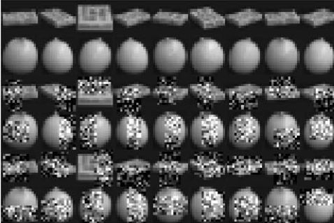
Figure 4: Original and noise sample images from Coil100 data set.

The recognition results of all methods on these data sets are listed in Table VII. From the table, we see on original data, the proposed CLDA has comparable performance to LDA-L1 and L2BLDA, and is better than LDA, RDA and RLDA. However, when noise is added, the performance of CLDA is barely affected, while performance of other methods is influenced by noise dramatically. The results show the robustness of CLDA, and it has better discriminant ability on noise data. We also list the ranks of various methods in Table VIII. The highest rank of CLDA on noise data supports its robustness.

To further investigate the behavior of CLDA under different reduced dimensions, Fig.5 describes the variation of accuracies of all methods along reduced dimensions. The figure shows that in general, as the number of dimensions varies, the accuracies for all methods in general arise. For LDA and RDA, due to their rank limit, their maximum number of reduced dimensions is restricted by $c-1$, where $c$ is the number of class. For Coil100 data set, the maximum number is 99. It should also be noted that for our CLDA, it may also encounter similar situation, since the number of reduced dimensions is decided by the rack of $\textbf{S}_{1}=\textbf{H}_{w}\textbf{F}\textbf{H}_{w}^{T}$ in (12). Then rank of $\textbf{S}_{1}$ is clearly related to $\textbf{H}_{w}$ and F, while F is changing during the solving procedure iteration. Therefore, the rank of $\textbf{S}_{1}$ is not deterministic. However, through experiments, we find out that CLDA can achieve high reduced dimensions. In fact, CLDA can extract the maximum number of reduced dimensions on original and 40% noise Coil100 data, and almost achieve maximum number on 30% noise Coil100 data, which is much lager than LDA and RDA. The results in Fig.5 show that reduced dimension has a great influence to the behavior of all methods, and it is necessary to choose an optimal one. Under optimal dimensions, the proposed CLDA behaves well.

TABLE VII: Classification results on Coil100 data.

Data set	LDA	RDA	RLDA	LDA-L1	L2BLDA	CLDA
Coil100ori	60.58	60.61	75.17	76.40	76.00	76.10
Coil100g30	57.84	57.34	70.82	73.66	71.88	77.38
Coil100g40	55.02	55.46	69.87	71.68	70.70	76.12

TABLE VIII: Classification ranks on Coil100 data.

Data set	LDA	RDA	RLDA	LDA-L1	L2BLDA	CLDA
	Rank	Rank	Rank	Rank	Rank	Rank
Coil100ori	6.0	5.0	4.0	1.0	3.0	2.0
Coil100g30	5.0	6.0	4.0	2.0	3.0	1.0
Coil100g40	6.0	5.0	4.0	2.0	3.0	1.0
Average rank	5.6667	5.3333	4.0000	1.6667	3.0000	1.3333

(a) Original data

(b) 30% noise data

(c) 40% noise data

Figure 5: The variation of accuracies along different dimensions on Coil100 data set.

IV-C2 USPS data set

We then consider USPS handwritten data set. USPS data set has 9298 digits images containing numbers 0-9, with each of them constituting a class. Each image is resized to 8$\times$8 pixel. Random 50% samples from each class are used for training, while the rest data are used for testing. To investigate the robustness of the proposed method, we further add ‘salt & pepper’ of noise density 0.05 on each training sample that covers 30% and 40% rectangular area of the image, as shown in Figure 6. We apply each dimensionality method on the above original and polluted training data, and obtain projection matrix. The classification results on test data are shown in Table IX, and the corresponding rank results are listed in Table X. From the tables, we see our CLDA outperforms other methods. To see the influence of reduced dimension to accuracy, we depict the variation of accuracies along dimensions in Fig.7. The highest accuracy on each data is also shown in the figure. From the figure, we see as the number of reduced dimensions increases, the accuracies of all methods have general upward trend. Also, selecting an optimal dimension is important to all methods. For all three cases, the proposed CLDA owns the highest accuracies under its optimal dimensions.

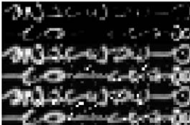
Figure 6: Original and noise sample images from USPS data set.

TABLE IX: Classification results on USPS data.

Data set	LDA	RDA	RLDA	LDA-L1	L2BLDA	CLDA
USPSori	90.60	91.56	84.79	94.22	93.81	94.62
USPSs30	90.97	90.66	88.52	94.13	93.68	94.49
USPSs40	91.78	90.69	88.88	93.12	93.59	94.37

TABLE X: Classification ranks on USPS data.

Data set	LDA	RDA	RLDA	LDA-L1	L2BLDA	CLDA
	Rank	Rank	Rank	Rank	Rank	Rank
USPSori	5.0	4.0	6.0	2.0	3.0	1.0
USPSs30	4.0	5.0	6.0	2.0	3.0	1.0
USPSs40	4.0	5.0	6.0	3.0	2.0	1.0
Average rank	4.3333	4.6667	6.0000	2.3333	2.6667	1.0000

(a) Original data

(b) 30% noise data

(c) 40% noise data

Figure 7: The variation of accuracies along different dimensions on USPS database.

V Conclusion

This paper introduced a capped $l_{p,q}$-norm for a matrix, where $p,q>0$, and proposed a novel linear discriminant analysis based on $l_{2,1}$-norm, named CLDA. Capped $l_{2,1}$-norm brought robustness to CLDA, and CLDA can be viewed as a weighted LDA. For a given $\epsilon$, the objective of CLDA was proved convergent. Experimental results showed that compared to related LDAs, CLDA can effectively remove extreme outliers and suppress the effect of noise data. How to determine an appropriate thresholding parameter in CLDA and investigate a more efficient algorithm are our future works. Extending CLDA to matrix and tensor data is also interesting. The corresponding Matlab code for CLDA can be downloaded from http://www.optimal-group.org/Resources/Code/CLDA.html.

References

- [1] Fisher R A. The use of multiple measurements in taxonomic problems. Annals of Eugenics, 1936, 7(2): 179-188.
- [2] Fukunaga K. Introduction to statistical pattern recognition, second edition. Academic Press, New York, 1991.
- [3] Zhang Z, Zhao M, Chow T W S. Constrained large margin local projection algorithms and extensions for multimodal dimensionality reduction. Pattern Recognition, 2012, 45(12): 4466-4493.
- [4] Zeiler S, Nicheli R, Ma N, et al. Robust audiovisual speech recognition using noise-adaptive linear discriminant analysis. IEEE International Conference on Acoustics, Speech and Signal Processing (ICASSP), 2016: 2797-2801.
- [5] Song X, Zheng Y, Wu X, et al. A complete fuzzy discriminant analysis approach for face recognition. Applied Soft Computing, 2010, 10(1): 208-214.
- [6] Raghavendra U, Acharya U R, Fujita H, et al. Application of Gabor wavelet and Locality Sensitive Discriminant Analysis for automated identification of breast cancer using digitized mammogram image. Applied Soft Computing, 2016, 46: 151-161.
- [7] Li C N, Shao Y H, Guo Y R, et al. Robust k-subspace discriminant clustering. Applied Soft Computing, 2019, 85: 105858.
- [8] Wang Z, Zhang G, Li D, et al. Locality sensitive discriminant matrixized learning machine. Knowledge-Based Systems, 2017, 116: 13-25.
- [9] Yin W, Ma Z. High order discriminant analysis based on Riemannian optimization. Knowledge-Based Systems, 2020: 105630.
- [10] Chen L F, Liao H Y M, Ko M T, et al. A new LDA-based face recognition system which can solve the small sample size problem. Pattern Recognition, 2000, 33(10): 1713-1726.
- [11] Yu H, Yang J. A direct LDA algorithm for high-dimensional data¡ªwith application to face recognition. Pattern Recognition, 2001, 34(10): 2067-2070.
- [12] Swets D L, Weng J J. Using discriminant eigenfeatures for image retrieval. IEEE Transactions on Pattern Analysis and Machine Intelligence, 1996, 18(8): 831-836.
- [13] Lai Z, Mo D, Wong W K, et al. Robust discriminant regression for feature extraction. IEEE Transactions on Cybernetics, 2018, 48(8): 2472-2484.
- [14] Randles R H, Broffitt J D, Ramberg J S, et al. Generalized linear and quadratic discriminant functions using robust estimates. Publications of the American Statistical Association, 1978, 73(363):564-568.
- [15] Guo Y, Hastie T, Tibshirani R. Regularized linear discriminant analysis and its application in microarrays. Biostatistics, 2006, 8(1): 86-100.
- [16] Hubert M, Van Driessen K. Fast and robust discriminant analysis. Computational Statistics & Data Analysis, 2004, 45(2): 301-320.
- [17] Yu S, Cao Z, Jiang X. Robust linear discriminant analysis with a Laplacian assumption on projection distribution. IEEE International Conference on Acoustics, Speech and Signal Processing (ICASSP), 2017: 2567-2571.
- [18] Kim S J, Magnani A, Boyd S. Robust Fisher discriminant analysis. Advances in Neural Information Processing Systems. 2005: 659-666.
- [19] Sugiyama M. Dimensionality reduction of multimodal labeled data by local Fisher discriminant analysis. Journal of Machine Learning Research, 2007, 8(1): 1027-1061.
- [20] Wang Z, Ruan Q, An G. Projection-optimal local Fisher discriminant analysis for feature extraction. Neural Computing and Applications, 2015, 26(3): 589-601.
- [21] Zhang Z, Chow T W S. Robust linearly optimized discriminant analysis. Neurocomputing, 2012, 79(3):140-157.
- [22] Okwonu F Z, Othman A R. Comparative performance of classical Fisher linear discriminant analysis and robust Fisher linear discriminant analysis. Matematika, 2013, 29: 213-220.
- [23] Zhong F, Zhang J. Linear discriminant analysis based on L1-norm maximization. IEEE Transactions on Image Processing, 2013, 22(8): 3018-3027.
- [24] Wang H, Lu X, Hu Z, et al. Fisher discriminant analysis with L1-norm. IEEE Transactions on Cybernetics, 2014, 44(6), 828-842.
- [25] Liu Y, Gao Q, Miao S, et al. A non-greedy algorithm for L1-norm LDA. IEEE Transactions on Image Processing, 2017, 26(2): 684-695.
- [26] Ye Q, Yang J, Liu F, et al. L1-norm distance linear discriminant analysis based on an effective iterative algorithm. IEEE Transactions on Circuits & Systems for Video Technology, 2018, 28(1): 114-129.
- [27] Chen X, Yang J, Jin Z. An improved linear discriminant analysis with L1-norm for robust feature extraction. The 22nd IEEE International Conference on Pattern Recognition, 2014: 1585-1590.
- [28] Li C N, Zheng Z R, Liu M Z, et al. Robust recursive absolute value inequalities discriminant analysis with sparseness. Neural Networks, 2017, 93: 205-218.
- [29] Li C N, Shao Y H, Yin W, etc. Robust and sparse linear discriminant analysis via an alternating direction method of multipliers. IEEE Transactions on Neural Networks and Learning Systems, 2020, 31(3): 915-926.
- [30] Zhang D, Sun Y, Ye Q, et al. Recursive discriminative subspace learning with L1-norm distance constraint. IEEE Transactions on Cybernetics, 2020, 50(5): 2138-2151.
- [31] Zheng W, Lin Z, Wang H. L1-norm kernel discriminant analysis via Bayes error bound optimization for robust feature extraction. IEEE Transactions on Neural Networks and Learning Systems, 2014, 25(4): 793-805.
- [32] Li C N, Shao Y H, Wang Z, et al. Robust Bhattacharyya bound linear discriminant analysis through an adaptive algorithm. Knowledge-Based Systems, 2019, 183: 104858.
- [33] Oh J H, Kwak N. Generalization of linear discriminant analysis using Lp-norm. Pattern Recognition Letters, 2013, 34(6): 679-685.
- [34] Ye Q, Fu L, Zhang Z, et al. Lp-and Ls-norm distance based robust linear discriminant analysis. Neural Networks, 2018, 105: 393-404.
- [35] Li C N, Shao Y H, Wang Z, et al. Robust bilateral Lp-norm two-dimensional linear discriminant analysis. Information Sciences, 2019, 500: 274-297.
- [36] Li C N, Shao Y H, Deng N Y. Robust L1-norm two-dimensional linear discriminant analysis. Neural Networks, 2015, 65: 92-104.
- [37] Chen S B, Chen D R, Luo B. L1-norm based two-dimensional linear discriminant analysis (In Chinese). Journal of Electronics and Information Technology, 2015, 37(6): 1372-1377.
- [38] Li M, Wang J, Wang Q, et al. Trace ratio 2DLDA with L1-norm optimization. Neurocomputing, 2017, 266(29): 216-225.
- [39] Li C N, Shang M Q, Shao Y H, et al. Sparse L1-norm two dimensional linear discriminant analysis via the generalized elastic net regularization[J]. Neurocomputing, 2019, 337: 80-96.
- [40] Ding C, Zhou D, He X, et al. R1-PCA: Rotational invariant L1-norm principal component analysis for robust subspace factorization. Proceedings of the 23rd International Conference on Machine Learning (ICML), June 2006.
- [41] Li X, Hu W, Wang H, et al. Linear discriminant analysis using rotational invariant L1 norm. Neurocomputing, 2010, 73(13-15): 2571-2579.
- [42] Nie F, Huang H, Cai X, et al. Efficient and robust feature selection via joint -norms minimization. Advances in Neural Information Processing Systems. 2010: 1813-1821.
- [43] Yang Z, Ye Q, Chen Q, et al. Robust discriminant feature selection via joint -norm distance minimization and maximization. Knowledge-Based Systems, 2020: 106090.
- [44] Lan G, Hou C, Yi D. Robust feature selection via simultaneous capped -norm and -norm minimization. 2016 IEEE International Conference on Big Data Analysis (ICBDA). IEEE, 2016: 1-5.
- [45] Ma X, Zhao M, Zhang Z, et al. Anchored projection based capped -norm regression for super-resolution. Pacific Rim International Conference on Artificial Intelligence. Springer, Cham, 2018: 10-18.
- [46] Zhao M, Zhang Z, Zhan C, et al. Graph based semi-supervised classification via capped -norm regularized dictionary learning. 2017 IEEE 15th International Conference on Industrial Informatics (INDIN). IEEE, 2017: 1019-1024.
- [47] Nie F, Wang X, Huang H. Multiclass capped -Norm SVM for robust classifications. Thirty-first AAAI Conference on Artificial Intelligence. 2017.
- [48] Gao H, Nie F, Cai W, et al. Robust capped norm nonnegative matrix factorization: Capped norm NMF. Proceedings of the 24th ACM International on Conference on Information and Knowledge Management. 2015: 871-880.
- [49] Zhang F, Yang Z, Chen Y, et al. Matrix completion via capped nuclear norm. IET Image Processing, 2018, 12(6): 959-966.
- [50] Sun Q, Xiang S, Ye J. Robust principal component analysis via capped norms. Proceedings of the 19th ACM SIGKDD International Conference on Knowledge Discovery and Data Mining. 2013: 311-319.
- [51] Sun W , Huang Y , Huang L , et al. -correlation and robust matching pursuit for sparse approximation. Digital Signal Processing, 2020, 104: 102761.
- [52] Yang X F, Shao Y H, Li C N, et al. Principal component analysis based on T-norm maximization. arXiv preprint arXiv:2005.12263, 2020.
- [53] Li T, Li M, Gao Q, et al. F-norm distance metric based robust 2DPCA and face recognition. Neural Networks, 2017, 94: 204-211.