Interpretable Representation Learning for Speech and Audio Signals Based on Relevance Weighting
Abstract
The learning of interpretable representations from raw data presents significant challenges for time series data like speech. In this work, we propose a relevance weighting scheme that allows the interpretation of the speech representations during the forward propagation of the model itself. The relevance weighting is achieved using a sub-network approach that performs the task of feature selection. A relevance sub-network, applied on the output of first layer of a convolutional neural network model operating on raw speech signals, acts as an acoustic filterbank (FB) layer with relevance weighting. A similar relevance sub-network applied on the second convolutional layer performs modulation filterbank learning with relevance weighting. The full acoustic model consisting of relevance sub-networks, convolutional layers and feed-forward layers is trained for a speech recognition task on noisy and reverberant speech in the Aurora-4, CHiME-3 and VOiCES datasets. The proposed representation learning framework is also applied for the task of sound classification in the UrbanSound8K dataset. A detailed analysis of the relevance weights learned by the model reveals that the relevance weights capture information regarding the underlying speech/audio content. In addition, speech recognition and sound classification experiments reveal that the incorporation of relevance weighting in the neural network architecture improves the performance significantly.
Index Terms:
Deep Representation Learning, Relevance Modeling, Raw Waveform Processing, Modulation Filtering, Acoustic-phonetics, Automatic Speech Recognition, Urban Sound Classification.I Introduction
Representation learning is the branch of machine learning that comprises of the methods that allow the learning of meaningful representations from raw data. With the growing interest in deep learning, representation learning using deep neural networks has been actively pursued [1]. The modalities like text and image have shown important successes for representation learning methods (for example, using word2vec models [2]). However, representation learning for speech data has been more challenging due to the temporal and intrinsic variabilities of the signals. Due to these challenges, the most common representation used in state-of-art speech recognition systems continues to be the mel spectrogram. In this paper, we explore representation learning for speech directly from the raw-waveform using a novel modeling approach.
The broad set of representation learning works in the speech domain can be categorized as supervised and unsupervised. In supervised setting, the main direction pursued has been the learning of the acoustic filterbank parameters from raw waveforms [3, 4, 5]. Compared to the acoustic models using the mel spectrogram features, these models are fed with raw speech signal and the first layer of the acoustic model performs a time-frequency decomposition of the signal. The supervised objective function is either a detection or a classification task [4, 6, 7]. In many of these cases, the initialization of the acoustic filter bank parameters are done using gammatone filters that closely approximate the hearing periphery [5, 7]. However, in spite of many of these efforts, the filter learning from raw waveform has not yielded performance improvements over the mel spectrogram features [7, 3].
For unsupervised learning of acoustic representations, Sailor et al. [8] investigated the use of restricted Boltzmann machines while Agrawal et al. [9] explored variational autoencoders. The wav2vec method proposed in [10] explored unsupervised pre-training for speech recognition by learning representations of raw audio. In our previous work, we had also explored modulation filter learning using an unsupervised objective function [11]. The approach of self-supervised learning (similar to the word2vec models for text) has also been pursued by Pascual et. al [12]. A comparison of several neural network architectures for modulation filter learning was also explored in [13].
In many of these previous approaches, the learned representations are assumed to capture distinctive speech features for phonetic discrimination. However, there has been limited attempts to explore the interpretability of the learned filterbanks. One exception is the SincNet filterbank [14] where the authors showed that the filter learning is resilient to the presence of band-limited noise. However, compared to vector representations of text which have shown to embed meaningful semantic properties, the interpretability of speech representations has been limited.
In this paper, we propose a relevance weighting mechanism that allows the interpretability of the learned representations in the forward propagation itself. The term “relevance weighting” comes from the text domain, where a static relevance weight is attached to each document, based on the relevance to the search term feature [15, 16]. A similar application of visual attention in the image domain uses spatial weighting to weight different parts of the image [17]. In this work, the term relevance weighting refers to the scheme of automatic weighting of the learned representations using a sub-network.
The proposed model consists of a two-step relevance weighting approach. The first step performs relevance weighting on the output of the first layer of convolutions. This convolutional layer learns a parametric acoustic filterbank from the raw waveform. The relevance weighted filterbank representation is used as input to the second convolutional layer which performs modulation filtering. This layer repeats the operations of the first layer in a 2-D fashion. The kernels of the second convolutional layer are 2-D spectro-temporal modulation filters and the filtered representations are weighted using another relevance sub-network. The rest of the neural network architecture performs the task of acoustic modeling for speech recognition. All the model parameters including the acoustic layer parameters, acoustic filterbank relevance sub-network, modulation filters and modulation relevance sub-network are learned in a supervised learning paradigm.
The subsequent analysis of the relevance sub-network reveals that the weights from the network contain information regarding the phonetic content of the label. The relevance weights are also adaptive to the presence of noise in the data. The automatic speech recognition (ASR) experiments are conducted on Aurora-4 (additive noise with channel artifact), CHiME-3 (additive noise with reverberation) and VOiCES (additive noise with reverberation) datasets. These experiments show that the learned representations from the proposed framework provide considerable improvements in ASR results over the baseline methods. The proposed representation learning framework is further extended to the task of urban sound classification (USC) on the Urbansound8K dataset where the goal is to classify short audio snippets into urban sound classes. In this task, the proposed approach shows improved classification performance and the weight analysis reveals distinctive audio characteristics that are captured by the relevance weighting scheme.
The rest of the paper is organized as follows. Section II details the motivation and related work. Section III describes the proposed two-step representation learning approach using relevance weighting. This is followed by interpretability analysis of the proposed representation learning in Section IV. Section V describes the ASR experiments with the various front-ends. The discussion of the model is given in Section VI. This is followed by a summary in Section VII.
II Motivation and Related work
One of the major motivation for the proposed modeling approach of relevance weighting is the evidence of gain enhancement mechanism in human sensory system. Both physiological and behavioral studies have suggested that stimulus-driven neural activity in the sensory pathways can be modulated in amplitude with attention [18]. The recordings of event-related brain potentials indicate that such sensory gain control or amplification processes play an important role in tasks that involve attention [19]. The combined event-related brain potential and neuroimaging experiments provide strong evidence that attentional gain control operates at an early stage of sensory processing [20]. These evidences support feature selection theories of attention and provide a basis for distinguishing between separate mechanisms of attentional suppression (of unattended inputs) and attentional facilitation (of attended inputs).
The second motivation comes from prior works on Mixture of Experts (MoE) models [21, 22]. For neural networks the work proposed by Shazeer et al. [23] explored multiple parallel neural networks followed by a gating network which performs a combination of the outputs from the networks. This MoE model showed significant promise for a language modeling task. The self attention module successfully inducted in transformer models [24] also incorporates information from multiple streams using a linear combination.
Inspired by these human and machine learning studies, the proposed relevance weighting attempts to model gain enhancement in a neural architecture. The frequency selectivity observed in auditory system can be modeled as relevance weighting in the acoustic filter bank layer while the cortical layer gain enhancement is attempted by modulating the relevance weights of the modulation filtering layer. While attention [24] and MoE models [23] attempt a combination of input streams that are fed to successive layers, the proposed relevance weighting merely performs a gain enhancement without a linear combination.
The learning of acoustic filterbank from raw waveform has been actively pursued in the last few years. The work reported by Palaz et al. proposed the use of convolutional neural networks on raw waveform to estimate phoneme class conditional probabilities [3]. Similarly, Sainath et al. [4] used power spectrum as input to convolutional neural network (CNN) to learn the filterbank features. For learning interpretable representations, the authors in [25] used Gaussian functions instead of mel-scale filterbanks with input being power spectra. The work proposed in [26] initializes the convolutional filters with Gabor wavelets before proceeding to learn the filter parameters. Ravanelli et al. [14] showed the use of sinc filters as parametric filters, with only the lower and higher cutoff frequencies learned from data. This work is extended in [12] to learn filterbank representations in a self-supervised framework.
The approach of modulation filter learning (modulation filters process the time-frequency representation as a 2-D image and perform filtering along time (rate) and frequency (scale) dimensions) using the linear discriminant analysis (LDA) has also been explored to learn the temporal modulation filters in a supervised manner [27, 28]. There have also been attempts to learn modulation filters in an unsupervised manner [29, 30, 31].
The performance of the learned representations from previous efforts has often been comparable to the mel-spectrogram features. However, most of the previous attempts do not allow the interpretation of the learned representations or their ability to capture relevant information.
III Relevance Weighting Based Representation Learning
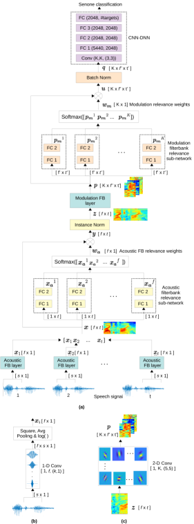
The block schematic of the proposed relevance weighting based representation learning is shown in Figure 1.
III-A Acoustic Filterbank Learning with Relevance Weighting
The first layer of the proposed model performs acoustic filtering from the raw waveforms using a convolutional layer. The input to the neural network are raw samples windowed into samples per frame. This frame of raw audio samples are processed with a 1-D convolution using kernels each of size . The kernels are modeled using a cosine-modulated Gaussian function [9],
| (1) |
where is the -th kernel (), is the center frequency (mean parameter) of the th kernel. The parametric approach to filterbank (FB) learning generates filters with a smooth frequency response. The Gaussian window has interesting properties of being smooth in time and frequency domain. In order to preserve the positive range of frequency values for , we choose the to be the sigmoid of a real number which is further scaled to half the sampling frequency of the signal. The mean parameters are updated in a supervised manner for each dataset. The convolution with the cosine-modulated Gaussian filters generates acoustic feature maps. These outputs are squared, average pooled within each frame and log transformed. This generates as dimensional features for each of the contextual frames, as shown in Figure 1. The matrix is interpreted as the “learned” time-frequency representation.
III-A1 Relevance weighting
The relevance weighting paradigm for acoustic FB layer is implemented using a relevance sub-network. This network is fed with the acoustic feature map of dimension for each of the Gaussian kernel (each row of the time-frequency representation ). A two layer deep neural network (DNN) with a dimensional input layer and a scalar output realizes the relevance sub-network. This operation is repeated for all the acoustic feature maps to generate as a dimensional vector with weights corresponding to each kernel. The relevance weights are generated using the softmax function as,
| (2) |
The weights are multiplied with each of the acoustic feature map (rows of ) to obtain the relevance weighted time-frequency representation . The relevance weights in the proposed framework are different from typical attention mechanism [32]. In the proposed framework, relevance weighting is applied over the representation as soft feature selection weights without a linear combination as done in attention models [32].
We also smooth the first stage outputs (weighted spectrogram of length time frames) using a normalization method inspired by instance norm principle [33, 34]. Let denote the relevance weighted time-frequency representation for frame () of kernel (). The soft weighted output is given as,
| (3) |
where is the sample mean of computed over and is the sample std. dev. of computed over . The constant acts as a relevance factor and is chosen as . The output of relevance weighting () is propagated to the subsequent layers for the acoustic modeling.
In our experiments, we use whose center frame is the senone target for the acoustic model. We also use kernels each of length . This value of corresponds to ms in time for a kHz sampled signal which has been found to be sufficient to capture temporal variations of a speech signal [35]. The value of is corresponding to ms window length and the frames are shifted every ms. The instance norm is not applied globally but rather applied on the given input patch of time frames (shown in Fig. 1). This corresponds to -second of length approximately. In our experiments, we also find that, after the normalization layer, the number of frames can be pruned to the center frames for the acoustic model training without loss in performance. This has significant computational benefits and the pruning is performed to keep only the frames around the center frame.
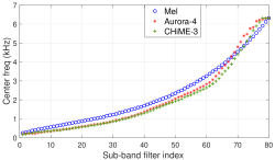
Figure 2 shows the center frequency ( values sorted in ascending order) of the acoustic filters obtained using multi-condition Aurora-4 (noisy) and CHiME-3 (noise and reverberations) datasets (details of the datasets are given in Section V) and this is compared with the center frequency of the conventional mel filterbank [36]. As can be observed, the proposed filterbank allocates more filters in lower frequencies compared to the mel filterbank. The CHiME-3 data contains reverberation artifacts which resulted in lower center frequencies compared to the noisy Aurora-4 data center frequency values.
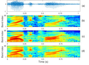
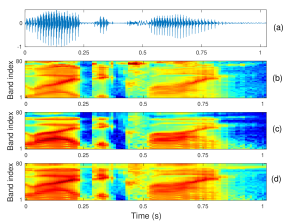
The soft relevance weighted time-frequency representation obtained from the proposed approach is shown in Figure 3(d) for an utterance with airport noise from Aurora-4 dataset (the waveform is plotted in Figure 3(a)). The corresponding mel spectrogram (without relevance weighting) is plotted in Figure 3(b). The time-frequency representation obtained through the learned filterbank (without relevance weighting) is plotted in Figure 3(c). It can be observed that, in the learned filterbank representations (Figure 3(c) and (d)), the formant frequencies are shifted upwards because of the increased number of filters in the lower frequency region. Also, the relevance weighting modifies the representations to preserve only the important details of the spectrogram.

III-B Modulation Filterbank Learning with Relevance Weighting
The representation from acoustic filterbank layer is fed to the second convolutional layer which is interpreted as modulation filtering layer (shown in Figure 1). Specifically, the modulation filter is characterized using the rate (temporal variations measured in Hz) and scale (spectral variations measured in cyc. per octave) dimensions.
The first layer (acoustic FB) generates time-frequency representations (2-D representations) as the output ( in Fig. 1). These 2-D representations are indexed by time-frame on x-direction and sub-band index in the y-direction. The sub-band indices are ordered in increasing value of center frequency which is required for modulation filtering in the second layer. The next stage of 2-D modulation filtering (rate-scale) is applied on 2-D time-frequency representation. The column of the time-frequency representation from the first layer constitutes a warped sampling of the spectrum from kHz with center frequencies shown in Figure 2. Hence, applying a filter along the y-direction of this 2-D time frequency representation constitutes scale filtering and the application of the filter along the x-direction constitutes rate filtering. Note that the sampling in the y-direction is non-linear in frequency.
In this work, we explore parametric and non-parametric approaches to modulation filter learning. In the parametric approach, the modulation filterbank (kernels of the modulation convolution layer) is designed as 2-D cosine-modulated Gaussian filters. Here, the ith 2-D filter with rate frequency and scale frequency is designed as:
| (4) |
with sampled at Hz (corresponding to ms hop in the time-frequency representation), sampled at cyc. per octave, and for modulation filters. The sign in the cosine term is used to incorporate upward and downward moving patterns in the input time-frequency representation. The cosine frequencies and are interpreted as rate and scale center frequencies in 2-D frequency response of the modulation filter. The means are the learnable parameters of the 2-D kernels and these are learned jointly with rest of the network parameters. We learn modulation feature maps using kernels of filter tap size.
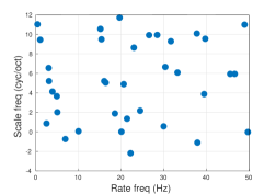
The learned center frequencies and (rate-scale) of the modulation filters are shown in Figure 4, from a model trained using Aurora-4 database. The rate frequency values span upto Hz, while the scale frequency can span from to cycles/octave. It can be observed from the plot that the learned filters span the rate-scale space with more density till around Hz rate frequency. The learned center frequencies span low scale regions with most of the filters in the cyc. per octave range. We begin with randomly spaced grid of rate-scale values (center frequency) as initialization and let the network update the center frequency values.

The modulation feature maps are pooled, leading to feature maps of size . These are weighted using a second relevance weighting sub-network (referred to as the modulation filter relevance sub-network in Figure 1). The input to the modulation relevance weighting sub-network is a modulation feature map of size and the model generates a scalar value for each of the feature maps. Let denote the dimensional vector from the output of modulation relevance sub-network. Similar to the acoustic relevance network, a softmax function is applied to generate modulation relevance weights ,
| (5) |
The weights are multiplied with the representation to obtain relevance weighted modulation feature maps . This weighting performs the adaptive selection of different modulation feature map representations (with different rate-scale characteristics). The resultant weighted representation is fed to the batch normalization layer [37]. The value of the normalization factor for batch norm is also chosen to be empirically. Following the acoustic filterbank layer and the modulation filtering layer (including the relevance sub-networks), the acoustic model consists of series of CNN and deep feed forward layers. The configuration details of different model parameters are given in Figure 1. The entire model is trained using the cross entropy loss with Adam optimizer [38].
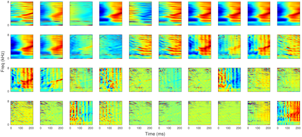
Figure 5 shows the obtained feature maps after the second stage of modulation filtering. The input to this layer is shown on left ( in Figure 1) and the obtained weighted feature maps ( in Figure 1) are plotted in the right. As can be observed, the modulation filtering layer filters the input patch using rate-scale filters with varying center frequencies.
The proposed two stage processing is loosely modeled based on our understanding of the human auditory system, where the cochlea performs acoustic frequency analysis while early cortical processing performs modulation filtering [39]. The relevance weighting mechanism attempts to model the feature selection/weighting inherently present in the auditory system (based on the relative importance of the representation for the downstream task).
IV Interpretability of the Representations
We analyze the representations and the relevance weights (outputs of acoustic relevance sub-network and modulation relevance sub-network) learned by the proposed model. The model architecture, shown in Figure 1, is trained using the Aurora-4 dataset. This model is tested using the TIMIT dataset (without any retraining). We use clean TIMIT as well as TIMIT dataset corrupted with noise [40]. The TIMIT dataset is hand labelled for phonemes, which allows the interpretation of the model representations based on the phoneme identity. For the analysis, the noisy TIMIT test set consisting of utterances is corrupted with different noise conditions, namely babble, exhall, restaurant and subway at different SNR levels, dB and dB SNR.
The phonemes are analyzed in two groups. A group of vowel phonemes {/ao/, /aa/, /ae/, /ey/, /iy/, /uw/} and a group of consonants from categories: plosives {/t/}, fricatives {/sh/, /zh/}, and nasals {/m/, /em/, /eng/}. The vowel sounds are also organized from back to front with regard to the place of articulation [41].

IV-A Mean Time-Frequency Representations
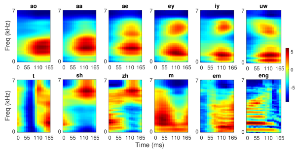
We analyze the learned time-frequency representation of each phoneme from the first layer (using the representation with previous and succeeding frames that cover ms duration). For example, the time-frequency representation of all /aa/ vowel exemplars (denoted as in Figure 1) are extracted from TIMIT utterances and are averaged to obtain one average time-frequency representation, as shown in Figure 6 (top row second column). For the computation of the average spectrogram for each phoneme, a contextual window of frames are chosen around the center frame (from every exemplar of that phoneme occurrence in the files) irrespective of the phone duration. Thus, all center frames belonging to a phoneme, except the two boundary frames on either side, are used in computing the average time-frequency representation of Figure 6.
The averaged time-frequency representation learned by the model reveals that mid/back vowels {/ao/, /aa/, /ae/} have relatively more concentrated activity at low to medium frequencies ( KHz), whereas front vowels {/ey/, /iy/} have two distinct peaks spaced over a larger frequency range around and kHz respectively. This is consistent with the known distribution of the three formants F1, F2, and F3 in these vowels [41]. On the other hand, while the plosive /t/, being a stop-consonant, has a time varying profile, the fricatives {/sh/, /zh/} have dominant energy at high frequencies and the nasal sounds {/m/, /em/} have energy at low to mid frequencies. Thus, the early representations learned by the model attempt to capture distinct phonetic properties. The purpose of this analysis is to relate the relevance weight plots that are analyzed in the following sections to the phonetic properties of the time-frequency representation.
IV-B Acoustic FB Relevance Weights
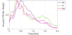
The acoustic filterbank relevance weights are analyzed to understand the weighting incorporated through the relevance sub-network. The relevance weights are averaged across the utterances for each phoneme and SNR level separately. Figure 7 shows the relevance weights for clean data and noisy data averaged over all the noise types.
As can be observed for clean and SNR of dB (low noise), for the front vowels {/ey/, /iy/, /uw/}, the filter indices that have the higher relevance weights lie in Hz range. For the mid/back vowels {/ao/, /aa/, /ae/}, more relevance is seen in the filter indices having center frequency above Hz. The filter indices with the highest relevance weights (peak marked with black star in Figure 7) tend to shift towards lower frequency as we move from the back vowel /ao/ to the front vowel /uw/. This is also very similar to the filter representations seen in the auditory system of ferrets and other mammals [41]. Also, in front/closed vowels {/iy/, /uw/}, the relevance weights show a second peak at the higher frequency index due to the presence of a higher formant frequency F3 (in the center frequency range of kHz). For the high noise condition (SNR dB), the relevance weights still preserve some of the phoneme specific selectivity although the weights tend to become more uniform across the frequency range. A more closer look at the relevance weights is given in Figure 8, where vowels are analyzed in clean conditions. As seen here, the peak activity moves from Hz to Hz as we move from back vowels to front vowels.
The acoustic filterbank (FB) relevance weights for consonants is shown in the second row of Figure 7. The plosive /t/ shows similar relevance weighting as observed in front vowels. The fricatives {/sh/, /zh/} show lesser sub-band selectivity compared to other phonemes (as these phonemes have significant high frequency activity as seen in Figure 6). The nasal sounds {/em/, /eng/} also elicit a large range of filter indices that have high relevance weights. Similar to the vowels, the decrease in SNR (higher noise case) reduces the selectivity of the representations as the relevance weights become more uniform. This is again similar to the human auditory processing where noise segregation happens to a very small degree in the peripheral time-frequency representation as compared to higher auditory cortical areas [42].
IV-C Modulation Filtering With Relevance Weighting
Figure 9 shows the bubble plot for modulation filter relevance weights for different phonemes (averaged over all respective exemplars of each phoneme). This plot is obtained by placing the relevance weight at the location of the center frequency (rate-scale) of the corresponding modulation filter. The size of the bubble is proportional to the magnitude of the corresponding relevance weight. The vowels and consonants are arranged in the same order as in acoustic FB relevance weight analysis. In order to highlight the contrast, we plot relevance weights for a given phoneme after subtracting the mean relevance weights over all the TIMIT phonemes.
The top row shows the weights for vowels under clean condition. It can be observed that almost all the vowels have higher contrast in relevance weight values for the rate frequency in Hz rate and to cyc./oct scale. Additionally, most of the back and mid vowels elicit higher contrast in weights for band-pass rate and low-pass scale frequencies. In the low SNR condition, for vowels (second row of Figure 9 with SNR dB), the relevance characteristics are much more intact compared to the acoustic FB layer relevance weights, with more contrast in lower rate regions. In case of consonants (third and fourth row of Figure 9), for the clean case, the plosive /t/ show similar trend as mid vowels while the fricative /sh/ show a low-pass rate + high-pass scale contrast profile. Additionally, most of the consonants have high contrast towards low-pass rate + high-pass scale and band-pass rate + low-pass scale region. On the other hand, the noisy consonants (SNR 0 dB) show low-pass rate profile scattered over different scale values.


V Experiments and results
The speech recognition system is trained using PyTorch toolkit [43] while the Kaldi toolkit [44] is used for decoding and language modeling. The models are discriminatively trained using the training data with cross entropy loss and Adam optimizer [38]. A hidden Markov model - Gaussian mixture model (HMM-GMM) system is used to generate the senone alignments for training the CNN-DNN based model. The ASR results are reported with a tri-gram language model and the best language model weight is obtained from the development set. The notation [A,M] refers to the model of learning acoustic and modulation filterbanks without relevance, [A-R,M] refers to the model that involves acoustic FB with relevance along with modulation FB without relevance, [A, M-R] refers to learning acoustic FB (with no relevance weighting), followed by modulation filter learning with relevance weighting, and [A-R,M-R] refers to the model with learning acoustic and modulation FB and having relevance weighting in both layers. The modulation filters are learnt in all baseline features as well as the first 2-D CNN layer.
For each dataset, we compare the ASR performance of the proposed approach with traditional mel filterbank energy (MFB) features, power normalized filterbank energy (PFB) features [45], RASTA features that perform modulation filtering (RAS) [46], and mean Hilbert envelope (MHE) features [47]. All the baseline features are processed with cepstral mean and variance normalization (CMVN) on a sec. running window. The baseline MFB features are directly fed to the 2-D modulation filtering layer (without the acoustic FB layer). The other baseline features like PFB, RAS and MHE also generate spectrogram like time-frequency representations which are used similar to the MFB features. For all these features, no relevance weighting is performed. The modulation filtering layer (M) is part of the baseline system and is present with all the other features like PFB, RAS, MHE (without explicit mention in all cases). An additional experiment, where relevance weighting is applied on the baseline MFB features (denoted as MFB-R) is also performed. For ASR experiments on the proposed model, we use a non-parametric approach in modulation filter learning. The non-parametric approach to modulation filtering involves learning 2-D kernels of the CNN layer that operates on the output of the acoustic FB layer. Empirically, the non-parametric modulation filters had a slight improvement over parametric modulation filters in ASR performance. The batch size of is chosen for all the model training using a learning rate of . The model training is performed for epochs after which the learning is found to saturate on the validation data.
| Cond | MFB,M | PFB,M | RAS,M | MHE,M | A-R,M-R |
|---|---|---|---|---|---|
| Aur-A : Clean with same Mic | |||||
| Clean | 4.2 | 4.0 | 5.3 | 3.8 | 3.6 |
| Aur-B : Noisy with same Mic | |||||
| Airport | 6.8 | 7.1 | 8.1 | 7.3 | 5.9 |
| Babble | 6.6 | 7.4 | 8.0 | 7.4 | 6.1 |
| Car | 4.0 | 4.5 | 4.8 | 4.3 | 3.9 |
| Rest. | 9.4 | 9.6 | 11.0 | 9.1 | 6.8 |
| Street | 8.1 | 8.1 | 9.4 | 7.6 | 6.9 |
| Train | 8.4 | 8.6 | 9.6 | 8.6 | 7.2 |
| \hdashlineAvg. | 7.2 | 7.5 | 8.5 | 7.4 | 6.1 |
| Aur-C : Clean with diff. Mic | |||||
| Clean | 7.2 | 7.3 | 9.0 | 7.3 | 6.0 |
| Aur-D : Noisy with diff. Mic | |||||
| Airport | 16.3 | 18.0 | 17.5 | 17.6 | 14.1 |
| Babble | 16.7 | 18.9 | 19.0 | 18.6 | 15.4 |
| Car | 8.6 | 11.2 | 10.5 | 9.6 | 7.7 |
| Rest. | 18.8 | 21.0 | 21.3 | 20.1 | 18.6 |
| Street | 17.3 | 19.5 | 18.5 | 18.8 | 16.8 |
| Train | 17.6 | 18.8 | 19.4 | 18.7 | 16.2 |
| \hdashlineAvg. | 15.9 | 17.9 | 17.7 | 17.3 | 14.8 |
| Avg. of all conditions | |||||
| Avg. | 10.7 | 11.7 | 12.2 | 11.4 | 9.6 |
V-A Aurora-4 ASR
Aurora-4 database consists of continuous read speech recordings of words corpus, recorded under clean and noisy conditions (street, train, car, babble, restaurant, and airport) at dB SNR. The training data has multi condition recordings ( speakers) with total hours of training data. The validation data has recordings for multi condition setup. The test data has recordings ( speakers) for each of the clean and noise conditions. The test data are classified into group Aur-A - clean data, Aur-B - noisy data, Aur-C - clean data with channel distortion, and Aur-D - noisy data with channel distortion.
The ASR performance on the Aurora-4 dataset is shown in Table I for each of the test conditions. As seen in the results, most of the noise robust front-ends do not improve over the baseline mel filterbank (MFB) performance. The proposed representation learning (two-stage relevance weighting) provides considerable improvements in ASR performance over the baseline system with average relative improvements of % over the baseline MFB features. Furthermore, the improvements in ASR performance are consistently seen across all the noisy test conditions.
V-A1 Statistical Significance
In order to compare how one system performs relative to the other in statistical sense, we use the bootstrap estimate for confidence interval [48]. This method computes a bootstrapping of word error rate (WER) values to extract the % confidence interval (CI), and also gives a probability of improvement (POI) for the system-in-test (system with the proposed representation learning) over the reference system (baseline system with MFB features). Table II shows the analysis for various test conditions in the Aurora-4 multi-condition training. The POI of the proposed system (A-R,M-R) system over the MFB is quite high for all the test conditions, with average POI being %.
| Test Cond. | Confidence Interval | POI (%) | |
|---|---|---|---|
| MFB,M | A-R,M-R | ||
| Aur-A | [4.1, 5.3 ] | [ 3.8, 5.0 ] | 95.1 |
| Aur-B | [ 7.3, 9.7 ] | [ 7.2, 9.4 ] | 86.8 |
| Aur-C | [ 7.7, 10.7 ] | [ 6.5, 9.1 ] | 99.0 |
| Aur-D | [ 17.4, 23.0 ] | [16.4, 21.8 ] | 95.3 |
| Avg | – | – | 94.0 |
| Cond. | MFB,M | PFB,M | RAS,M | MHE,M | A-R,M | A-R,M-R |
|---|---|---|---|---|---|---|
| Dev | ||||||
| Sim | 12.9 | 13.3 | 14.7 | 13.0 | 12.5 | 12.0 |
| Real | 9.9 | 10.7 | 11.4 | 10.2 | 9.9 | 9.6 |
| \hdashlineAvg. | 11.4 | 12.0 | 13.0 | 11.6 | 11.2 | 10.8 |
| Eval | ||||||
| Sim | 19.8 | 19.4 | 22.7 | 19.7 | 19.2 | 18.5 |
| Real | 18.3 | 19.2 | 20.5 | 18.5 | 17.3 | 16.6 |
| \hdashlineAvg. | 19.1 | 19.3 | 21.6 | 19.1 | 18.2 | 17.5 |
V-B CHiME-3 ASR
The CHiME-3 corpus for ASR contains multi-microphone tablet device recordings from everyday environments, released as a part of 3rd CHiME challenge [49]. Four varied environments are present - cafe (CAF), street junction (STR), public transport (BUS) and pedestrian area (PED). For each environment, two types of noisy speech data are present - real and simulated. The real data consists of -channel recordings of sentences from the WSJ corpus spoken in the environments listed above. The simulated data was constructed by artificially mixing clean utterances with environment noises. The training data has (real) noisy recordings and simulated noisy utterances, constituting a total of hours. We use the beamformed audio in our ASR training and testing. The development (dev) and evaluation (eval) data consists of and utterances respectively. For each set, the sentences are read by four different talkers in the four CHiME-3 environments. This results in () and () real development and evaluation utterances.
The results for the CHiME-3 dataset are reported in Table III. The approach of acoustic FB learning with relevance weighting alone (A-R) improves over the baseline system (MFB) as well as the other noise robust front-ends considered here. The proposed approach of 2-stage relevance weighting over learned acoustic representations and modulation representations (A-R,M-R) provides significant improvements over baseline features. On the average, the proposed approach provides relative improvements of % over MFB features in the eval set. The detailed results on different noises in CHiME-3 are reported in Table IV. For most of the noise conditions in CHiME-3 in simulated and real environments, the proposed approach provides consistent improvements over the baseline features.
| Dev Data | Eval Data | |||||||
| Cond. | MFB,M | A-R,M-R | MFB,M | A-R,M-R | ||||
| Sim | Real | Sim | Real | Sim | Real | Sim | Real | |
| BUS | 10.9 | 11.6 | 10.9 | 11.3 | 13.7 | 22.5 | 13.0 | 21.4 |
| CAF | 16.8 | 9.8 | 14.7 | 9.5 | 22.3 | 18.8 | 19.6 | 16.1 |
| PED | 10.4 | 8.0 | 9.6 | 7.5 | 20.8 | 17.7 | 18.7 | 15.4 |
| STR | 13.8 | 10.3 | 13.0 | 10.0 | 22.5 | 14.4 | 22.7 | 13.3 |
V-C VOiCES ASR
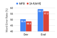
The Voices Obscured in Complex Environmental Settings (VOiCES) corpus is a creative commons speech dataset [50], being used as part of VOiCES Challenge [51]. The training data set of hours has utterances sampled at kHz from speakers, with each utterance having s segments of read speech from the Librispeech corpus. We performed a 1-fold reverberation and noise augmentation of the data using Kaldi [44]. The ASR development set consists of hours of distant recordings from the VOiCES dev speakers. It contains recordings from microphones. The evaluation set consists of hours of distant recordings from the VOiCES eval speakers and contains recordings from microphones from an unseen room. The ASR performance of VOiCES dataset with baseline MFB features and our proposed approach of 2-step relevance weighting is reported in Figure 10. These results suggest that the proposed model is also scalable to relatively larger ASR tasks with large vocabulary where consistent improvements are obtained with the proposed approach in addition to the interpretability of the representations learned.
| Features | ASR (WER in %) | ||||
|---|---|---|---|---|---|
| Aur-A | Aur-B | Aur-C | Aur-D | Avg. | |
| MFB,M | 4.2 | 7.2 | 7.2 | 15.9 | 10.7 |
| A,M (Acoustic FB) | 4.1 | 6.8 | 7.3 | 16.2 | 10.7 |
| MFB-R,M | 4.0 | 7.3 | 7.1 | 16.1 | 10.8 |
| A-R,M | 3.6 | 6.4 | 8.1 | 15.1 | 10.0 |
| A,M-R | 3.4 | 6.1 | 7.9 | 16.9 | 10.4 |
| MFB-R, G-R | 3.7 | 6.3 | 6.4 | 15.1 | 10.3 |
| A-R,M-R | 3.6 | 6.1 | 6.0 | 14.8 | 9.6 |
| [A-R,M-R] Learned on | ASR Trained and Tested on | ||
|---|---|---|---|
| Aurora-4 | CHiME-3 | VOiCES | |
| Aurora-4 | 9.6 (10.7) | 14.3 (15.3) | 57.6 (59.1) |
| CHiME-3 | 9.7 | 14.2 | 59.0 |
| VOiCES | 9.9 | 14.4 | 57.2 |
VI Discussion
VI-A Effect of relevance weighting on different stages
We compare the ASR performance of the proposed approach of 2-stage relevance weighting (A-R,M-R) with the learned acoustic FB representation (A) without any relevance weighting, relevance weighting on fixed mel filterbank features (MFB-R), acoustic FB relevance weighting without modulation FB relevance weighting (A-R), and modulation relevance weighting alone on learned time-frequency representation (A,M-R). We also report performance with handcrafted filterbanks at both the stages, denoted as [MFB-R, G-R]. The hand-crafted modulation filters (G) were chosen as 2-D cosine-modulated Gaussian filters with pre-determined rate-scale center frequencies. Based on prior studies, we use more filters in the band-pass rate and low pass scale regions.
The results are reported in Table V averaged for test conditions of Aurora-4 dataset. Since the modulation filtering layer (M) is part of the baseline system and is present with all the features, the notation ‘M’ alone is omitted in discussion. As can be observed, the acoustic FB features (A) performs similar to the MFB baseline features on average. The MFB-R features, which denote the application of the relevance weighting over mel filterbank features, does not provide improvements over baseline MFB features. The relevance weighted features A-R improves over the acoustic FB (A) features with average relative improvements of %. The features (A,M-R) having modulation relevance weighting alone improves over baseline in condition Aur-A and Aur-B, while there is degradation in Aur-C and Aur-D. The handcrafted features (MFB-R,G-R) also improves over the baseline. The proposed 2-stage relevance weighting (A-R,M-R) provides improvements in all test conditions over the baseline.
VI-B Representation transfer across tasks
In a subsequent analysis, we perform a cross-domain ASR experiment, i.e., we use the proposed representation learning (A-R,M-R) learned from one of the datasets (either Aurora-4, CHiME-3 or VOiCES challenge) to train/test ASR on the other dataset. All other layers in Figure 1 are learned using the in-domain ASR. The results of these cross-domain representation learning and ASR training experiments are reported in Table VI. The performance reported in this table are the average WER on each of the datasets. The results shown in Table VI illustrate that the representation learning process is relatively robust to the domain of the training data, which suggest that the proposed representation learning approach can be generalized for other “matched” tasks (especially between Aurora-4 and VOiCES tasks).
| Features without relevance weighting | ASR |
| MFB,M (mel filterbank) | 10.7 |
| A,M (our cosine modulated Gaussian filterbank) | 10.7 |
| Sinc,M (sinc filterbank from [14]) | 10.8 |
| Features with relevance weighting | ASR |
|---|---|
| MFB-R,M-R | 10.6 |
| A-R,M-R | 9.6 |
| Sinc-R,M-R | 10.0 |
| ANP-R,M-R | 11.6 |
| A-SelfAttn,M | 10.8 |
VI-C Comparison with other learnable front-end methods
To compare the proposed approach in this work with the SincNet method [14], we replace our cosine modulated Gaussian filterbank with the sinc filterbank as kernels in first convolutional layer. The baseline ASR system with sinc filterbank is trained jointly without any relevance weighting and the rest of the architecture is kept the same as shown in Fig. 1. The ASR system with sincFB and 2-stage relevance weighting is also trained. In addition, we also compare with acoustic FB learning in a non-parametric (ANP) manner (learning the 1-D CNN kernels directly from raw input without using a cosine modulated Gaussian function) [3, 5, 7].
The ASR performance is reported in Table VII for mel filterbank features (MFB), our proposed cosine modulated Gaussian filterbank without relevance weighting (R) and the sinc filterbank from [14] (Sinc). For the experiments without relevance weighting, it can be observed that the parametric sinc filterbank performs similar to our acoustic filterbank, and both perform similar to mel filterbank. The relevance weighting over sinc FB (Sinc-R,M-R) improves over the baseline with average relative improvement of around % over MFB, while the proposed [A-R,M-R] representation improves over the sinc FB approach. The proposed parametric approach to acoustic FB learning also improves over the non-parametric (ANP) approach.
In addition, to compare the relevance weighting approach with the self-attention approach, we train an ASR model with the acoustic FB relevance sub-network replaced with self-attention module (with self-attention weighting on sub-bands) for the acoustic filterbank layer. From the ASR performance for this system (A-SelfAttn,M), it can be observed that the relevance weighting proposed in this work is superior to channel weighting based on self-attention.
VI-D Unsupervised vs. Supervised representation learning
In our proposed approach, the parametric kernels of the acoustic FB layer can be initialized in different ways; (i) initialization using unsupervised training of CVAE [9], (ii) unsupervised initialization + supervised fine tuning in ASR, and (iii) random initialization + supervised fine tuning. Table VIII shows the effects of acoustic FB initialization on ASR. All the features are trained with the proposed relevance weighting based model. For the random initialization, we sample the center frequencies uniformly at random or use a sigmoidal mapping function on the uniform random variable. It can be observed that unsupervised initialization alone of acoustic FB parameters (and no fine tuning) does not improve over baseline. The random initialization of acoustic FB followed by supervised fine-tuning for ASR gives considerable improvement in ASR performance. The random initialization of acoustic FB means on sigmoidal frequency scale performs better than the uniform scale with no fine tuning. The approach of unsupervised initialization with supervised fine-tuning (approach followed in this paper) gives the best ASR performance among all choices considered here.
VI-E Choice of hyper-parameters
We experiment with various choices of hyper-parameters in acoustic FB learning. The effect of context length of the input patch () is analyzed through ASR performance with the proposed [A-R, M-R] approach. The Aurora-4 dataset is used with different context length of , , , and . From the results reported in Table IX, it can observed that the performance improves with increasing the context length, with the best performance for and .
We also observe the effect of acoustic filter length . While ms yields a frequency resolution of Hz, a ms long kernel has a frequency resolution of Hz and a ms long kernel has a frequency resolution of Hz. The baseline features like mel filter bank use windowing in the frequency domain with mel-spaced filters. The filters in the lower frequency range in the mel-scale have higher resolution (around Hz). From Table X, it can be observed that while the shorter filter length degrades the ASR performance, the increased filter length beyond ms does not improve the ASR performance.
| Type of acoustic FB learning | ASR |
|---|---|
| Random Initialization on uniform scale + No fine tuning | 11.9 |
| Random Initialization on sigmoidal frequency scale + No fine tuning | 11.2 |
| Unsupervised Initialization (& no fine tuning) | 10.9 |
| Unsupervised Initialization + supervised fine tuning | 9.6 |
| Random Initialization on sigmoidal scale + supervised fine tuning | 9.9 |
| Context length (value of ) | ASR (WER in %) |
|---|---|
| 21 | 10.2 |
| 51 | 10.1 |
| 81 | 10.0 |
| 101 | 9.6 |
| 131 | 9.6 |
| Filter length (value of ) | ASR (WER in %) |
|---|---|
| 64 (ms) | 10.6 |
| 128 (ms) | 9.6 |
| 256 (ms) | 9.7 |
VI-F Urban Sound Classification
The spectro-temporal characteristics of the different types of audio signals are different, and hence, the learned time-frequency representation should capture these distinctive properties for efficient sound classification. The proposed two stage approach of representation learning is explored for urban sound classification task. The same architecture used for speech (shown in Figure 1) is used for audio representation learning. The input to the network is a short audio snippet and the network is trained for classifying urban sound classes. Following the acoustic FB layer and the modulation filtering layer (with the two relevance weighting sub-networks), the model consists of a CNN-LSTM for the USC task (the LSTM backend provided an improved performance for the USC task but not for the ASR task).
| Rep. | Accuracy (%) | ||||||||||
|---|---|---|---|---|---|---|---|---|---|---|---|
| AI | CA | CH | DO | DR | EN | GU | JA | SI | ST | Avg | |
| MFB,M | 32 | 61 | 50 | 65 | 45 | 44 | 54 | 44 | 66 | 61 | 52 |
| A,M | 32 | 67 | 60 | 68 | 63 | 55 | 82 | 48 | 71 | 65 | 58 |
| A-R,M-R | 40 | 62 | 60 | 68 | 66 | 56 | 79 | 59 | 74 | 67 | 62 |
| M3[52] | - | - | - | - | - | - | - | - | - | - | 58 |

VI-F1 Dataset
The USC system is trained using PyTorch [43] using UrbanSound8K dataset [53]. It contains sound clips sampled at kHz, with duration up to s divided into sound classes: air conditioner (AI), car horn (CA), children playing (CH), dog bark (DO), drilling (DR), engine idling (EN), gun shot (GU), jackhammer (JA), siren (SI), and street music (ST). The best trained model is chosen through cross-validation loss. In our work, we use folds for training purpose, and the results are reported with average of -fold cross validation.
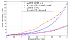
Fig. 11 shows the center frequency ( values sorted in ascending order) of the acoustic filters obtained for the USC task. A comparison with the mel filter center frequencies as well as learnt center frequency from Aurora-4 speech data is also provided for reference. The center frequency of learned filters in audio data deviate from the mel counterparts. In particular, the learned representations have more emphasis on higher frequencies compared to the mel spectrogram.
Table XI reports the average USC performance for baseline system and the proposed two-stage approach of representation learning. As seen in the results, the learnt acoustic FB features (A) alone (without any relevance weighting) performs considerably better than the fixed MFB features, with an absolute improvement of %. The 2-stage (A-R,M-R) approach further gives improvement in almost all the classes with absolute improvement of % on average over baseline MFB system. In addition, the results are better than the very deep CNN model (M3) with large number of kernels () on raw audio waveform reported in [52].
VI-F2 Analysis
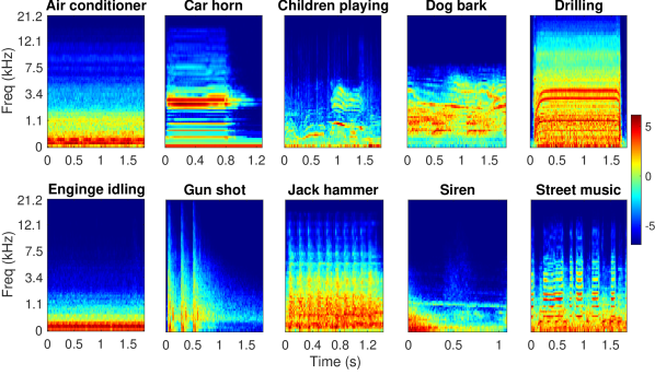
For the audio sounds in the Urbansound8K dataset, we analyze the learned time-frequency representation of each class in Fig. 13. As seen here, air conditioner, engine idling and siren sounds have mostly low frequency content. The car horn, drilling and street music sounds have multiple peaks at different frequencies. The drilling and jack hammer sounds have higher frequency range spanning till kHz.
The acoustic FB relevance weights for the audio signals are analyzed in Fig. 12. It can be observed that most of the sounds exhibit higher relevance weight for low to mid acoustic frequencies, with drilling and jackhammer sounds having significant weight values till the end of the spectral range. The air conditioner and engine idling are low frequency sounds with peak primarily in between Hz. The car horn, siren and street music sounds exhibit multiple frequencies and hence, have higher value for relevance weights till around kHz. The gun-shot sound weight profile exhibits an exclusive peak at around Hz.
VI-G Contributions Beyond Prior Works
The self-attention approach [54] applies a fixed neural layer on inputs (typically hidden layer activations indexed by time) to generate a single scalar value. A softmax operation applied on the scalar values over time provides the attention weights. The attention weights are used to generate a linear combination of the embeddings. In the proposed work, while a softmax operation on scalar relevance weight values are performed, we do not perform any linear combination of the inputs. Thus, the scalar values act as a relevance weights (gain) that modulate the information flow to the subsequent layers. A higher value of the weight signifies more relevance to the corresponding input stream (sub-band in acoustic FB layer or modulation filter in the modulation FB layer). In addition, self-attention in LSTM networks are typically performed at the end of the encoding layers (closer to the target layer) or as multiple modules of self-attention in transformer networks [24] which carry all the way upto the target layers. In the proposed framework, the relevance weighting is only performed in the initial layers which are closer to the input representations. Hence, the relevance weights offer interpretability in terms of speech/audio characteristics.
The gated neural network approach [23] explored multiple parallel “expert” networks followed by a gating network which performs a convex combination of the outputs from the networks. Again, similar to self-attention, the model only propagates the combined output.
The ASSERT network [55] for spoof detection proposes an attention filtering layer. This approach operates on speech spectrograms of the entire utterance (typically few seconds) and generates an attentional heat-map using a deep convolutional neural network with a U-net model containing multiple levels of dialation, downsampling and upsampling layers along with skip connections. The attentional heat-map is then element wise multiplied on the input utterance spectrogram and added with input spectrogram. The entire model is trained for spoof detection task. In the proposed approach, the model does not generate a heat-map on all components. It rather provides a scalar relevance weight for each sub-band (acoustic FB layer) or for each modulation filter (modulation FB layer). In addition, the proposed model does not add the weighted input again with the input but rather propagates the weighted feature stream directly to the subsequent layers. Further, the authors in ASSERT use the attention filtering only on the input log-magnitude spectrogram. The ASSERT attention filtering will be more cumbersome than the proposed approach when incorporated in modulation filtering layers as the attentional heat-map needed would be 3-D in nature.
VII Summary
In this paper, we have proposed a framework for relevance weighting based representation learning from raw waveform.
VII-A Key Contributions
The key contributions of the work can be summarized as follows:
-
•
Posing the representation learning problem in an interpretable filterbank learning framework using relevance weighting mechanism from raw waveform.
-
•
Using a two-step process for learning representations: first step to obtain time-frequency (spectrogram) representation from raw waveform; second step to perform modulation filtering on first step output. Both steps have separate relevance weighting sub-networks, which are differentiable and can be easily integrated in the backpropagation learning.
-
•
Implementing the acoustic filterbank in the first convolutional layer of the proposed model using a parametric cosine-modulated Gaussian filter bank whose parameters are learned. A relevance sub-network provides relevance weights to acoustic FB.
-
•
The second convolutional layer performs modulation filtering over the first layer output. Another relevance sub-network provides relevance weights to the modulation feature maps.
-
•
ASR experiments on a variety of speech datasets containing noise and reverberation showing the benefits of the proposed approach.
-
•
Analysis of the relevance weights reveal that the weights capture underlying phonetic content in speech.
-
•
The proposed 2-stage framework is extended to urban sound classification task where it shows improved performance. The weight analysis reveals that distinct audio characteristics are captured by the relevance weights. 111The implementation of the proposed approach is available at https://github.com/PurviAgrawal/Interpretable_rawWaveform_relevanceWeighted
VII-B Limitations
Some limitations of the proposed work include,
-
•
The proposed approach is empirical. The model is proposed and analyzed based on performance metrics.
-
•
The total number of parameters in the mel-scale baseline is around M while in the proposed approach the number of trainable parameters is M. In terms of total number of parameters involved, the proposed approach only increases the number of parameters by %. In terms of computational time, we performed an experiment with test files from the Aurora-4 corpus and measured the computation time for forward pass through the model for the baseline system as well as the proposed relevance weighted model. The computation time for the proposed model increased by % (sec. of computational time for the proposed method versus sec. for the baseline mel-spec system).
VII-C Future Work
The relevance weighting should also incorporate some level of feedback if the proposed model is to imitate biology in true sense. In addition, other gross statistics of the signal maybe potentially useful in deriving the relevance weights. Furthermore, extending the approach to representation learning for other machine learning tasks like speaker recognition and language modeling are part of future considerations.
References
- [1] Y. Bengio, A. Courville, and P. Vincent, “Representation learning: A review and new perspectives,” IEEE transactions on pattern analysis and machine intelligence, vol. 35, no. 8, pp. 1798–1828, 2013.
- [2] T. Mikolov, K. Chen, G. Corrado, and J. Dean, “Efficient estimation of word representations in vector space,” Proc. of International Conference on Learning Representations (ICLR), arXiv preprint arXiv:1301.3781, 2013.
- [3] D. Palaz, R. Collobert, and M. M. Doss, “Estimating phoneme class conditional probabilities from raw speech signal using convolutional neural networks,” Proceedings of Interspeech, pp. 1766–1770, 2013.
- [4] T. N. Sainath, B. Kingsbury, A. R. Mohamed, and B. Ramabhadran, “Learning filter banks within a deep neural network framework,” in IEEE Workshop on Automatic Speech Recognition and Understanding (ASRU), 2013, pp. 297–302.
- [5] Z. Tüske, P. Golik, R. Schlüter, and H. Ney, “Acoustic modeling with deep neural networks using raw time signal for LVCSR,” in Proc. of Interspeech, 2014, pp. 890–894.
- [6] Y. Hoshen, R. J. Weiss, and K. W. Wilson, “Speech acoustic modeling from raw multichannel waveforms,” in IEEE International Conference on Acoustics, Speech and Signal Processing (ICASSP), 2015, pp. 4624–4628.
- [7] T. N. Sainath, R. J. Weiss, A. Senior, K. W. Wilson, and O. Vinyals, “Learning the speech front-end with raw waveform CLDNNs,” in Proc. of Interspeech, 2015, pp. 1–5.
- [8] H. B. Sailor and H. A. Patil, “Filterbank learning using convolutional restricted boltzmann machine for speech recognition.” in IEEE International Conference on Acoustics, Speech and Signal Processing (ICASSP), 2016, pp. 5895–5899.
- [9] P. Agrawal and S. Ganapathy, “Unsupervised raw waveform representation learning for ASR,” Proc. of Interspeech 2019, pp. 3451–3455, 2019.
- [10] S. Schneider, A. Baevski, R. Collobert, and M. Auli, “wav2vec: Unsupervised pre-training for speech recognition,” Proc. of Interspeech, pp. 3465–3469, 2019.
- [11] P. Agrawal and S. Ganapathy, “Deep variational filter learning models for speech recognition,” in IEEE International Conference on Acoustics, Speech and Signal Processing (ICASSP), 2019, pp. 5731–5735.
- [12] S. Pascual, M. Ravanelli, J. Serrà, A. Bonafonte, and Y. Bengio, “Learning problem-agnostic speech representations from multiple self-supervised tasks,” arXiv preprint arXiv:1904.03416, 2019.
- [13] P. Agrawal and S. Ganapathy, “Comparison of unsupervised modulation filter learning methods for asr.” in INTERSPEECH, 2018, pp. 2908–2912.
- [14] M. Ravanelli and Y. Bengio, “Interpretable convolutional filters with SincNet,” in Proc. of Neural Information Processing Systems (NIPS), 2018.
- [15] S. E. Robertson and K. S. Jones, “Relevance weighting of search terms,” Journal of the American Society for Information science, vol. 27, no. 3, pp. 129–146, 1976.
- [16] S. E. Robertson and S. Walker, “On relevance weights with little relevance information,” in Proc. of the 20th annual international ACM SIGIR Conference on Research and development in information retrieval, 1997, pp. 16–24.
- [17] K. Xu, J. Ba, R. Kiros, K. Cho, A. Courville, R. Salakhudinov, R. Zemel, and Y. Bengio, “Show, attend and tell: Neural image caption generation with visual attention,” in International Conference on Machine Learning (ICML), 2015, pp. 2048–2057.
- [18] J. Kauramäki, I. P. Jääskeläinen, and M. Sams, “Selective attention increases both gain and feature selectivity of the human auditory cortex,” PLoS One, vol. 2, no. 9, p. e909, 2007.
- [19] J. de Boer and K. Krumbholz, “Auditory attention causes gain enhancement and frequency sharpening at successive stages of cortical processing—evidence from human electroencephalography,” Journal of cognitive neuroscience, vol. 30, no. 6, pp. 785–798, 2018.
- [20] S. A. Hillyard, E. K. Vogel, and S. J. Luck, “Sensory gain control (amplification) as a mechanism of selective attention: electrophysiological and neuroimaging evidence,” Philosophical Transactions of the Royal Society of London. Series B: Biological Sciences, vol. 353, no. 1373, pp. 1257–1270, 1998.
- [21] R. A. Jacobs, M. I. Jordan, S. J. Nowlan, and G. E. Hinton, “Adaptive mixtures of local experts,” Neural computation, vol. 3, no. 1, pp. 79–87, 1991.
- [22] M. I. Jordan and R. A. Jacobs, “Hierarchical mixtures of experts and the em algorithm,” Neural computation, vol. 6, no. 2, pp. 181–214, 1994.
- [23] N. Shazeer, A. Mirhoseini, K. Maziarz, A. Davis, Q. Le, G. Hinton, and J. Dean, “Outrageously large neural networks: The sparsely-gated mixture-of-experts layer,” ICLR, 2017. [Online]. Available: arXivpreprintarXiv:1701.06538
- [24] A. Vaswani, N. Shazeer, N. Parmar, J. Uszkoreit, L. Jones, A. N. Gomez, Ł. Kaiser, and I. Polosukhin, “Attention is all you need,” in Advances in neural information processing systems, 2017, pp. 5998–6008.
- [25] H. Seki, K. Yamamoto, and S. Nakagawa, “A deep neural network integrated with filterbank learning for speech recognition,” in IEEE International Conference on Acoustics, Speech and Signal Processing (ICASSP), 2017, pp. 5480–5484.
- [26] N. Zeghidour, N. Usunier, I. Kokkinos, T. Schaiz, G. Synnaeve, and E. Dupoux, “Learning filterbanks from raw speech for phone recognition,” in IEEE International Conference on Acoustics, Speech and Signal Processing (ICASSP), 2018, pp. 5509–5513.
- [27] S. Van Vuuren and H. Hermansky, “Data-driven design of RASTA-like filters.” in Eurospeech, vol. 1, 1997, pp. 1607–1610.
- [28] J.-W. Hung and L.-S. Lee, “Optimization of temporal filters for constructing robust features in speech recognition,” IEEE Transactions on Audio, Speech, and Language Processing, vol. 14, no. 3, pp. 808–832, 2006.
- [29] P. Agrawal and S. Ganapathy, “Modulation filter learning using deep variational networks for robust speech recognition,” IEEE Journal of Selected Topics in Signal Processing, vol. 13, no. 2, pp. 244–253, 2019.
- [30] H. B. Sailor and H. A. Patil, “Unsupervised learning of temporal receptive fields using convolutional RBM for ASR task,” in European Signal Processing Conference (EUSIPCO). IEEE, 2016, pp. 873–877.
- [31] P. Agrawal and S. Ganapathy, “Unsupervised modulation filter learning for noise-robust speech recognition,” Journal of the Acoustical Society of America, vol. 142, no. 3, pp. 1686–1692, 2017.
- [32] Y. Zhang, P. Zhang, and Y. Yan, “Attention-based LSTM with multi-task learning for distant speech recognition,” Proc. of Interspeech, pp. 3857–3861, 2017.
- [33] D. E. Rumelhart, G. E. Hinton, and R. J. Williams, “Learning representations by back-propagating errors,” Nature, vol. 323, no. 6088, p. 533, 1986.
- [34] D. Ulyanov, A. Vedaldi, and V. Lempitsky, “Instance normalization: The missing ingredient for fast stylization,” arXiv preprint arXiv:1607.08022, 2016.
- [35] M. S. Lewicki, “Efficient coding of natural sounds,” Nature neuroscience, vol. 5, no. 4, pp. 356–363, 2002.
- [36] S. Davis and P. Mermelstein, “Comparison of parametric representations for monosyllabic word recognition in continuously spoken sentences,” IEEE Transactions on Acoustics, Speech, and Signal Processing, vol. 28, no. 4, pp. 357–366, 1980.
- [37] S. Ioffe and C. Szegedy, “Batch normalization: Accelerating deep network training by reducing internal covariate shift,” Proc. of International Conference on Machine Learning (ICML), pp. 448–456, 2015.
- [38] D. P. Kingma and J. Ba, “Adam: A method for stochastic optimization,” Proc. of International Conference on Learning Representations (ICLR), arXiv preprint arXiv:1412.6980, 2015.
- [39] N. Mesgarani, M. Slaney, and S. A. Shamma, “Discrimination of speech from nonspeech based on multiscale spectro-temporal modulations,” IEEE Transactions on Audio, Speech, and Language Processing, vol. 14, no. 3, pp. 920–930, 2006.
- [40] J. S. Garofolo, L. F. Lamel, W. M. Fisher, J. G. Fiscus, and D. S. Pallett, “DARPA TIMIT acoustic-phonetic continous speech corpus,” NASA STI/Recon technical report, vol. 93, 1993.
- [41] N. Mesgarani, S. V. David, J. B. Fritz, and S. A. Shamma, “Phoneme representation and classification in primary auditory cortex,” The Journal of the Acoustical Society of America, vol. 123, no. 2, pp. 899–909, 2008.
- [42] S. Da Costa, W. van der Zwaag, L. M. Miller, S. Clarke, and M. Saenz, “Tuning in to sound: frequency-selective attentional filter in human primary auditory cortex,” Journal of Neuroscience, vol. 33, no. 5, pp. 1858–1863, 2013.
- [43] A. Paszke, S. Gross, S. Chintala, and G. Chanan, “PyTorch,” Computer software. Vers. 0.3, vol. 1, 2017.
- [44] D. Povey et al., “The KALDI speech recognition toolkit,” in IEEE ASRU, no. EPFL-CONF-192584. IEEE Signal Processing Society, 2011.
- [45] C. Kim and R. M. Stern, “Power-normalized cepstral coefficients (PNCC) for robust speech recognition,” in IEEE International Conference on Acoustics, Speech and Signal Processing (ICASSP), 2012, pp. 4101–4104.
- [46] H. Hermansky and N. Morgan, “RASTA processing of speech,” IEEE Transactions on Speech and Audio Processing, vol. 2, no. 4, pp. 578–589, 1994.
- [47] S. O. Sadjadi, T. Hasan, and J. H. Hansen, “Mean Hilbert envelope coefficients (MHEC) for robust speaker recognition,” in Proc. of Interspeech, 2012.
- [48] M. Bisani and H. Ney, “Bootstrap estimates for confidence intervals in asr performance evaluation,” in IEEE International Conference on Acoustics, Speech, and Signal Processing (ICASSP), 2004, pp. 409–412.
- [49] J. Barker, R. Marxer, E. Vincent, and S. Watanabe, “The third ‘CHiME’ speech separation and recognition challenge: Dataset, task and baselines,” in IEEE Workshop on Automatic Speech Recognition and Understanding (ASRU), 2015, pp. 504–511.
- [50] C. Richey, M. A. Barrios, Z. Armstrong, C. Bartels, H. Franco, M. Graciarena, A. Lawson, M. K. Nandwana, A. Stauffer, J. van Hout et al., “Voices obscured in complex environmental settings (VOiCES) corpus,” Proc. of Interspeech, pp. 1566–1570, 2018.
- [51] M. K. Nandwana, J. Van Hout, C. Richey, M. McLaren, M. A. Barrios, and A. Lawson, “The VOiCES from a distance challenge 2019,” Proc. of Interspeech, pp. 2438–2442, 2019.
- [52] W. Dai, C. Dai, S. Qu, J. Li, and S. Das, “Very deep convolutional neural networks for raw waveforms,” in IEEE International Conference on Acoustics, Speech and Signal Processing (ICASSP). IEEE, 2017, pp. 421–425.
- [53] J. Salamon, C. Jacoby, and J. P. Bello, “A dataset and taxonomy for urban sound research,” in Proceedings of the 22nd ACM international conference on Multimedia, 2014, pp. 1041–1044.
- [54] Z. Lin, M. Feng, C. N. d. Santos, M. Yu, B. Xiang, B. Zhou, and Y. Bengio, “A structured self-attentive sentence embedding,” arXiv preprint arXiv:1703.03130, 2017.
- [55] C.-I. Lai, N. Chen, J. Villalba, and N. Dehak, “Assert: Anti-spoofing with squeeze-excitation and residual networks,” arXiv preprint arXiv:1904.01120, 2019.
![[Uncaptioned image]](/html/2011.02136/assets/x21.jpg) |
Purvi Agrawal is a PhD scholar at Learning and Extraction of Acoustic Patterns (LEAP) lab, Electrical Engineering, Indian Institute of Science (IISc), Bangalore. Prior to joining IISc, she obtained her Master of Technology in Communications from DA-IICT, Gandhinagar in 2015. She obtained her Bachelor of Technology in Electronics and Communication from College of Technology and Engineering, Udaipur in 2013. She has also worked in Sony R & D Labs, Tokyo in 2017. Her research interests include machine learning for signal processing, unsupervised learning and applications, and robust speech recognition. She is a student member of IEEE. |
![[Uncaptioned image]](/html/2011.02136/assets/Sriram2.png) |
Sriram Ganapathy is a faculty member at the Electrical Engineering, Indian Institute of Science, Bangalore, where he heads the activities of the learning and extraction of acoustic patterns (LEAP) lab. Prior to joining the Indian Institute of Science, he was a research staff member at the IBM Watson Research Center, Yorktown Heights. He received his Doctor of Philosophy from the Center for Language and Speech Processing, Johns Hopkins University. He obtained his Bachelor of Technology from College of Engineering, Trivandrum, India and Master of Engineering from the Indian Institute of Science, Bangalore. He has also worked as a Research Assistant in Idiap Research Institute, Switzerland from 2006 to 2008. At the LEAP lab, his research interests include signal processing, machine learning methodologies for speech and speaker recognition and auditory neuro-science. He is a subject editor for the Speech Communications journal and a senior member of the IEEE. |