MBB: Model-Based Baseline for Global Guidance of Model-Free Reinforcement Learning via Lower-Dimensional Solutions

Abstract

One spectrum on which robotic control paradigms lie is the degree in which a model of the environment is involved, from methods that are completely model-free such as model-free RL, to methods that require a known model such as optimal control, with other methods such as model-based RL somewhere in the middle. On one end of the spectrum, model-free RL can learn control policies for high-dimensional (hi-dim), complex robotic tasks through trial-and-error without knowledge of a model of the environment, but tends to require a large amount of data. On the other end, “classical methods” such as optimal control generate solutions without collecting data, but assume that an accurate model of the system and environment is known and are mostly limited to problems with low-dimensional (lo-dim) state spaces. In this paper, we bring the two ends of the spectrum together. Although models of hi-dim systems and environments may not exist, lo-dim approximations of these systems and environments are widely available, especially in robotics. Therefore, we propose to solve hi-dim, complex robotic tasks in two stages. First, assuming a coarse model of the hi-dim system, we compute a lo-dim value function for the lo-dim version of the problem using classical methods (eg. value iteration and optimal control). Then, the lo-dim value function is used as a baseline function to warm-start the model-free RL process that learns hi-dim policies. The lo-dim value function provides global guidance for model-free RL, alleviating the data inefficiency of model-free RL. We demonstrate our approach on two robot learning tasks with hi-dim state spaces and observe significant improvement in policy performance and learning efficiency. We also give an empirical analysis of our method with a third task.

I Introduction

Methods for obtaining robot control policies can be considered to lie somewhere on a spectrum of the degree to which a model of the system and environment is needed or used. Model-free reinforcement learning (RL) [1] and classical methods with known models such as optimal control [2] stand at the two extremes of spectrum, with model-based RL being somewhere in the middle. In this paper, we aim to combine the two extremes to achieve benefits of both.

Model-free RL does not need a model and only relies on environment experience (that is, data collection) to learn a policy, and has gained popularity for solving high-dimensional, complex tasks [3, 4]. By mapping observations to actions via a neural network, model-free RL allows the control policies to be learned directly from high-dimensional (hi-dim) inputs [1, 5]. However, it is often data-inefficient, requiring an impractically large number of trials to learn desired behaviours, which can be costly and unrealistic in robotics.

“Classical methods”, on the other hand, derive a control policy without the need for data as long as a known, accurate model of the system is available. For example, optimal control is a classical method and has been widely used in various robotic applications [6, 7]. Accurate models are available for many robotic systems, and thus optimal control can provide optimal solutions to many tasks without collecting any data from the environment [8]. However, optimal control is often limited to low-dimensional (lo-dim) problems and lacks computational scalability to complex tasks with hi-dim state spaces, especially when one aims to derive a control policy from raw sensor input.

In this work, we study how lo-dim solutions obtained from classical methods can provide global guidance to model-free RL to learn hi-dim policies in a data-efficient way. Note that this is unlike model-based RL [9, 10] which aims to improve data efficiency by learning an model of environment dynamics, which can be difficult in hi-dim cases. Instead, we demonstrate that using solutions of lo-dim problems with known, lo-dim models can be simple yet effective in warm-starting model-free RL and can make model-free RL more data-efficient in hi-dim tasks than even model-based RL.

Specifically, we propose Model-Based Baseline (MBB), a novel approach that improves data efficiency of model-free RL on hi-dim problems by leveraging solutions from associated lo-dim problems. This is accomplished by first obtaining a lo-dim value function by solving a simplified, lo-dim version of the hi-dim problem using classical methods. The lo-dim value function is then used in the hi-dim problem to initialize the baseline function for model-free RL in a supervised fashion. We use value iteration and optimal control as two representative classical methods for obtaining lo-dim value functions.

Two practical advantages of MBB are as follows. First, many robotic system models [11, 12] are widely used in classical methods like control theory on lo-dim applications for many years, so a plethora of lo-dim models can be used. Second, solving lo-dim problems with classical methods are very “cheap” from a computational and data perspective. Therefore, lo-dim solutions can greatly improve data efficiency of model-free RL, even when the hi-dim environment dynamics is difficult to obtain or even learn [13, 14].

MBB complements existing methods that use policy priors from expert [15, 16] or classical control methods [17, 18] as guidance. By initializing the baseline function, we in a sense provide a prior on the value function. Even when no other warm-start, exploration, or reward shaping methods are used, our proposed method can enable successful training of complex control policies.

We evaluate our approach on two common mobile robotic tasks, and obtain significant improvements in both policy performance and learning efficiency. We offer an empirical analysis of our approach in terms of policy gradient estimation with a third task.

II Preliminaries

II-A RL Notations and Terminologies

Consider a Markov Decision Process (MDP) with an agent and environment state space $S$, a set of agent actions $A$, a probability of transition (at any time $t$) from a state $s$ in $S$ to another state $s^{\prime}$ in $S$ under action $a$ in $A$: $P_{a}(s,s^{\prime})=\mathrm{Pr}(s_{t+1}=s^{\prime}|s_{t}=s,a_{t}=a)$ and an immediate reward $r(s_{t},a_{t})$. In this paper, we simplify the reward function as $r(s_{t})$ so that it only depends on current state $s_{t}$. To match notations of the approximate system dynamics discussed in Sec. III, we introduce a slight abuse of notation $s_{t+1}\sim f(s_{t},a_{t})$ to denote that $s_{t+1}$ is drawn from the distribution $\mathrm{Pr}(s_{t+1}=s^{\prime}|s_{t}=s,a_{t}=a)$.

The policy $\pi(a|s)$ specifies the probability that the agent will choose action $a$ in state $s$. The trajectory $\tau$ is a sequence of states and actions $\tau=\left(s_{0},a_{0},s_{1},a_{1},\ldots\right)$ in the environment, and the discounted return $R(\tau)=\sum_{t=0}^{\infty}\gamma^{t}r(s_{t})$ describes the discounted sum of all rewards obtained by the agent, with discount factor $\gamma\in[0,1]$. We denote the on-policy value function as $V^{\pi}(s)$, which gives the expected return starting in state $s$ and always acting according to policy $\pi$. Given an MDP, we aim to find a policy $\pi$ to maximize the expected return $J(\pi)=\underset{\tau\sim\pi}{\mathrm{E}}[R(\tau)]$.

II-B Baseline in Policy Gradient Estimation

In this paper, we consider model-free RL with policy gradient optimization. More specifically, we consider actor-critic methods and assume a generic form of policy gradient given by Eq. (1) [19]

$$\small\nabla_{\theta}J\left(\pi_{\theta}\right)=\underset{\tau\sim\pi_{\theta}}{\mathrm{E}}\left[\sum_{t=0}^{T}\nabla_{\theta}\log\pi_{\theta}\left(a_{t}\mid s_{t}\right)\left(G_{t}^{\lambda}-b(s_{t})\right)\right],$$ (1)

where $G_{t}^{\lambda}$ is the TD$(\lambda)$ return [20] considering weighted average of $n$-step returns for $n=1,2,...\infty$ via parameter $\lambda$. In Eq. (1), $b(s_{t})$ is called baseline function and it potentially reduces the variance without changing the expectation of policy gradient estimation [21]. One common choice of $b(s_{t})$ in actor-critic RL is the on-policy value function $V^{\pi}(s_{t})$ that approximates the expected return, which provides the lowest variance [21]. In general, actor-critic RL initialize $V^{\pi}(s_{t})$ randomly and update it by solving a nonlinear regression problem $\small\operatorname{min}_{\phi}\sum_{t=1}^{T}\left\|V_{\phi}^{\pi}\left(s_{t}\right)-G^{\lambda}_{t}\right\|^{2}$, where $\phi$ are on-policy value function parameters. Empirically, the choice $b(s_{t})=V^{\pi}(s_{t})$ results in more stable policy learning compared to other choices. However, as we will demonstrate, this may not always be the best choice, especially when a large amount of initial exploration is needed.

II-C Value Iteration

The value function $V^{\pi}$ corresponding to any policy $\pi$ can be computed by iteratively applying Bellman backup [22] until convergence, as shown in Eq. (2) where $k$ is the iteration index. This procedure is a form of value iteration, a classical dynamic programming-based method that is often applied in lo-dim state spaces.

$$\small V_{k+1}^{\pi}(s)=\sum_{a\in A}\pi(a|s)(r(s,a)+\gamma\sum_{s^{\prime}\in S}{P(s^{\prime}|s,a)\cdot V_{k}^{\pi}(s^{\prime})})$$ (2)

The computational complexity of value iteration restricts its use on many complicated RL tasks despite the theoretical guarantee on convergence. However, our proposed method can take advantage of value iteration as a classical method to solve a lo-dim version of a hi-dim problem and uses the resulting value function to initialize the baseline of the hi-dim problem. The choice of $\pi$ in Eq. (2) is flexible and can be chosen to balance between RL exploration and exploitation. We use the Boltzmann policy [23] in this paper.

II-D Model Predictive Control

Model Predictive Control (MPC) is a classical control-theoretic method that uses a model of a system to predict the system’s future behaviours and optimizes a given cost function, possibly subject to input and state constraints [24, 25]. Typically, MPC is done in a receding horizon fashion, and involves repeatedly observing the current state at each time step $t$, then solving for the sequence of states and controls over a look-ahead horizon $H$ that satisfies a constrained planning problem, and executing the first element of the control sequence. In this paper we consider a MPC problem that addresses a collision avoidance task with smooth nonlinear constraints, as provided in [26].

In addition to value iteration, we take the MPC solutions of a simplified problem with a lo-dim system model, and use it to initialize a baseline function for a associated hi-dim RL problem. The use of MPC scales our approach to the problems in which even the simplified system models are too hi-dim to be tractably solved by value iteration or other dynamic programming-based methods.

III Model-Based Baseline (MBB)

In this paper, we propose a model-informed baseline function $b(\cdot)=V^{\mathrm{M}}(\cdot)$ that can substitute the on-policy value function $V^{\pi}(\cdot)$ as a novel baseline function to provide global guidance to model-free RL. The primary purpose of our baseline function is not to minimize variance of policy gradient estimation as $V^{\pi}(\cdot)$ does [21], but to give better policy update directions with fewer samples in certain challenging situations.

We first introduce notations and terminologies used in this section. We use the phrase “full MDP model” to refer to the state transition $f(s,a)$ used in the hi-dim target RL problem $\Omega$, $s$ as full state and observation and $a$ as action. For every $\Omega$, we denote its counterpart, a simplified, lo-dim problem as $\tilde{\Omega}$, which involves an approximate, lo-dim model $\tilde{f}(\mathrm{x,u})$, $\mathrm{x}$ as lo-dim state and $u$ as control. We denote baseline function for $\Omega$ as $V^{\mathrm{M}}(s)$, which is initialized by the value function $\tilde{V}^{\mathrm{M}}(\mathrm{x})$ of $\tilde{\Omega}$. We use the term “warm-start” to refer to the process of obtaining a value function $\tilde{V}^{\mathrm{M}}(\mathrm{x})$ from the lo-dim problem $\tilde{\Omega}$, and using it to initialize the baseline function $V^{\mathrm{M}}(s)$ of the hi-dim problem $\Omega$.

We now present our Model-Based Baseline (MBB) approach. Our algorithm starts with choosing a simplified, approximate system model $\tilde{f}(\cdot)$, which should be relatively lo-dim but captures the key system behaviors of the hi-dim target RL problem. Such a simple model is usually not difficult to obtain since they have been well developed for many classical control methods [27, 7]. Then, we employ either value iteration or optimal control (e.g. MPC) to solve the simplified problem $\tilde{\Omega}$ with system model $\tilde{f}(\cdot)$ to collect training data $\mathcal{D}:=\{(s_{i},\tilde{V}^{\mathrm{M}}(\mathrm{x}_{i})|i=0,1,2,...\}$. $\mathcal{D}$ contains the mapping between states in $\Omega$ and approximate values in $\tilde{\Omega}$, and is used to initialize the model-based baseline $V^{\mathrm{M}}_{\eta_{0}}(s)$. Starting with a randomly initialized policy $\pi_{\theta_{0}}$, we begin updating policy parameters $\theta_{0}$ with any actor-critic RL algorithms using our baseline $V^{\mathrm{M}}_{\eta_{0}}(s)$. At each iteration $k$, we use the policy gradient $\nabla_{\theta}J\left(\pi_{\theta}\right)$ obtained from online trajectories $\mathcal{T}_{k}$ to update policy parameters $\theta_{k}$, and optionally update the baseline parameter $\eta_{k}$ based on a novel criterion. Algorithm 1 summarizes our method.

Algorithm 1 MBB: Model-Based Baseline

1:  Select an approximate model $\tilde{f}(\cdot)$ for the target RL problem $\Omega$ and a corresponding simplified problem $\tilde{\Omega}$ modelled by $\tilde{f}(\cdot)$.

2:  Apply classical methods to solve $\tilde{\Omega}$ to collect dataset $\mathcal{D}:=\{(s_{i},\tilde{V}^{\mathrm{M}}(\mathrm{x}_{i})|i=0,1,2,...\}$.

3:  Initialize the model-based baseline $b(s)=V^{\mathrm{M}}_{\eta_{0}}(s)$ via supervised learning on $\mathcal{D}$. Initialize policy $\pi_{\theta_{0}}$ randomly.

4:  for $k=0,1,2,...$ do

5:     Collect trajectories $\mathcal{T}_{k}=\{\tau_{j}|j=0,1,2,...\}$ by running policy $\pi_{k}=\pi_{\theta_{k}}$ in the target hi-dim problem $\Omega$.

6:     Calculate TD$(\lambda)$ return $G_{t}^{\lambda}$ and the baseline $V^{\mathrm{M}}(s_{t})$ for every $s_{t}$ to estimate policy gradient $\nabla_{\theta}J\left(\pi_{\theta}\right)$ from Eq. (1).

7:     Update policy $\theta_{k+1}=\theta_{k}+\alpha_{k}\nabla_{\theta}J\left(\pi_{\theta}\right)$.

8:     Optionally update the baseline parameter $\eta_{k}$ based on the criterion defined in Eq. (9) and Eq. (10).

9:  end for

III-A Model Selection

“Model selection” refers to choosing an approximate, lo-dim system model for the target RL problem with hi-dim state space to efficiently compute value function based on it. In many complex RL problem where the state input is hi-dim, the full MDP model $f(\cdot)$ is often inaccessible or difficult to learn since it captures the evolution of hi-dim state inputs including both sensor data and robot internal state. However, an approximate system model ${\tilde{f}(\cdot)}$ is often known and accessible. This is especially true in robotics if knowledge of a robotic system’s approximate dynamics is available. The tilde implies it is not necessary for ${\tilde{f}(\cdot)}$ to perfectly reflect the real state transitions $f(\cdot)$. In fact, ${\tilde{f}(\cdot)}$ should typically be lo-dim to allow for efficient value computation, while still capturing key robot physical dynamics.

To better distinguish $f(\cdot)$ and $\tilde{f}(\cdot)$: $f(\cdot)$ is unknown but runs behind the target RL problem $\Omega$ as underlying transition model, e.g. the built-in simulator model; while $\tilde{f}(\cdot)$ is empirically selected as an approximate model to calculate the lo-dim $\tilde{V}^{\mathrm{M}}(\cdot)$ to warm-start the baseline function $V^{M}(\cdot)$. We emphasize that it is common to have a model of a robotic system. For example, car-like systems may be modeled using a Dubins car or extended Dubins car, as in Eq. (5) and Eq. (6). In addition, as we will show in Sec. IV, even a very simple, approximate model can provide a baseline function that greatly improves learning efficiency.

The connection between the full MDP and the approximate system model is formalized via the state, described by Eq. (3). We define surjective function $\mathcal{F}$ to establish an onto correspondence from $s$ to $\mathrm{x}$. Particularly, in this paper we consider $\mathcal{F}$ to be a selection matrix mapping denoted by $\mathbf{M}$, which can be chosen based on system knowledge to ensure that $\mathrm{x}$ captures the key aspects of robot physical dynamics. While a discussion involving more general forms of $\mathcal{F}$ can be interesting, we leave it as future work, and focus on the providing of global guidance of hi-dim RL using lo-dim value functions.

$$\mathrm{x}=\mathcal{F}(s)=\mathbf{M}s$$ (3)

The approximate system state $\mathrm{x}$ evolves according to a known, lo-dim model $\tilde{f}(\cdot)$, where $\tilde{f}(\cdot)$ can be in the form of ODE as in Eq. (4a), MDP as in Eq. (4b), or any other model as long as there is a method to efficiently solve the lo-dim problem.

$$\dot{\mathrm{x}}(t)=\tilde{f}(\mathrm{x}(t),u(t))$$ (4a)

$$\mathrm{P}_{u}(\mathrm{x}_{t},\mathrm{x}_{t+1})=\mathrm{Pr}(\mathrm{x}_{t+1}|\mathrm{x}_{t},u_{t})$$ (4b)

For example, in the simulated car example shown in Sec. IV-A, the full state $s=(x,y,\theta,d_{1},...,d_{8})$ includes the position $(x,y)$, heading $\theta$, as well as eight laser range measurements $d_{1},\ldots,d_{8}$ that provide distances from nearby obstacles. As one can imagine, the evolution of $s$ can be very difficult if $f(\cdot)$ is impossible to obtain, especially in a priori unknown environments. By following Eq. (3) and choosing the selection matrix $\mathbf{M}=\left[\begin{array}[]{ll}\mathbf{I}_{3\times 3}&\mathbf{0}_{3\times 10}\end{array}\right]$, the state of the approximate system $\mathrm{x}$ can be constructed to contain the robotic internal state $\mathrm{x}=(x,y,\theta)$, and evolves according to Eq. (4). In this case, we can choose the Dubins Car model, a very common kinematic model of cars and aircraft flying in the horizontal plane [6, 27], to be the approximate system dynamics, given in Eq. (5). As we will show, such simple dynamics are sufficient for improving data efficiency in model-free RL. We assume the access of necessary information of environment, e.g. the positions and sizes of obstacles, only when we solve the lo-dim problem.

$$\small\dot{\mathrm{x}}=\begin{bmatrix}\dot{x}\\ \dot{y}\\ \dot{\theta}\\ \end{bmatrix}=\begin{bmatrix}v\cos\theta\\ v\sin\theta\\ \omega\\ \end{bmatrix}$$ (5)

$$\small\dot{\mathrm{x}}=\begin{bmatrix}\dot{x}\\ \dot{y}\\ \dot{\theta}\\ \dot{v}\\ \dot{\omega}\\ \end{bmatrix}=\begin{bmatrix}v\cos\theta\\ v\sin\theta\\ \omega\\ \alpha_{v}\\ \alpha_{\omega}\end{bmatrix}$$ (6)

The choice of the approximate system model representing the real robot may be very flexible, depending on what behaviours one wishes to capture. In the 3D ODE model given in Eq. (5), the focus is on modelling how the change in the position of the car must be aligned with the heading $\theta$. However, if other variables – in this case linear and angular speed $v$, $\omega$ for example – are deemed crucial for the task under consideration, one may also choose a more complex 5D approximate system given in Eq. (6), where we have $\mathrm{x}=(x,y,\theta,v,\omega)$ In principle, a good choice of approximate model should be computationally tractable for the lo-dim value function computation, and should capture the system behaviours that are important for performing the desired task.

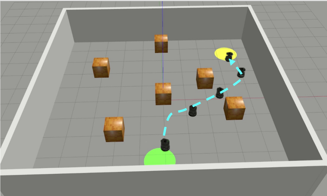
(a) VI-fixed

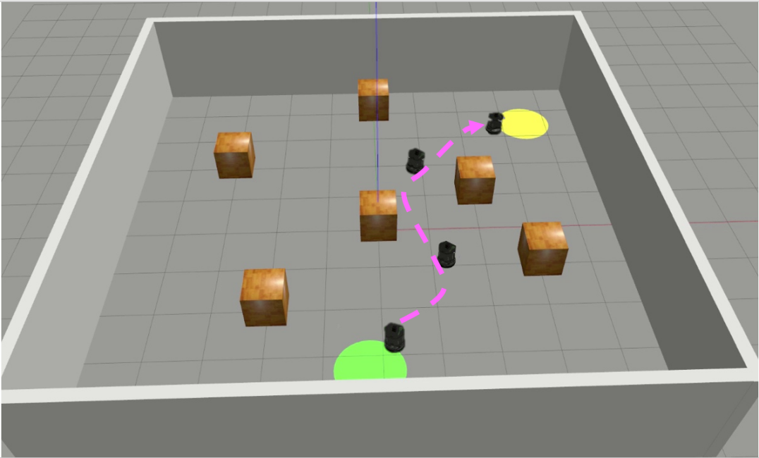
(b) MPC-fixed

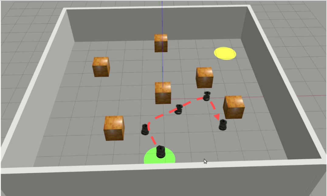
(c) Baseline Approach

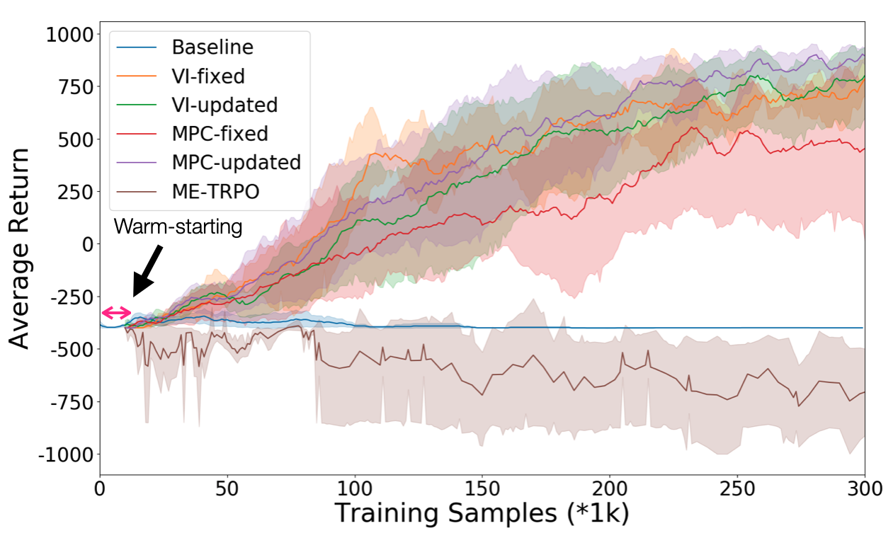
(d) Overall Performance

Figure 1: Simulated car trajectories from final policies using (a) VI-fixed (b) MPC-fixed and (c) Baseline approach. Both variants of MBB approach successfully learn a collision-free, goal-reaching policy while the baseline approach learns to conservatively move in free space while avoiding obstacles but never getting to the goal. (d) Overall performance comparison on the car example. The black arrow refers to MBB warm-starting period, which is approximately $\mathrm{10K}$ training samples. During this period the baseline approach starts RL process while MBB does not. Including this results in a fair comparison on learning efficiency between the baseline and MBB approach.

III-B Training Data Generation

We generate supervision data $\{s_{i},\tilde{V}^{\mathrm{M}}(\mathrm{x}_{i})\}$ to train a model-based baseline function $b(s)=V^{\mathrm{M}}(s)$ for the target RL problem $\Omega$ with a hi-dim state space. The state $s_{i}$ can be obtained by directly sampling from $\Omega$ while $\tilde{V}^{\mathrm{M}}(\mathrm{x}_{i})$ is obtained by plugging in $\mathrm{x}_{i}=\mathbf{M}s_{i}$ into $\tilde{V}^{\mathrm{M}}(\cdot)$, which can be computed using value iteration or MPC on a lo-dim problem $\tilde{\Omega}$ with a selected approximate system model $\tilde{f}(\cdot)$. We now outline two examples.

III-B1 Value Iteration Solution

We first consider a simple case, where the robotic system model $\tilde{f}(\cdot)$ is sufficiently lo-dim, typically no more than 4D. This is because as a dynamic programming-based method, the computational complexity of value iteration scales exponentially with system dimensionality.

For instance, a differential drive robot simulated in this work can be approximately modelled as a 3D system using Eq. (5). To apply value iteration on it, we discretize the state $\mathrm{x}=(x,y,\theta)$ and action $u=(v,\omega)$ space, derive a corresponding discrete time model using finite difference method like Forward Euler, and repeatedly calculate the value for each discrete state $\mathrm{x}$ following Eq. (2) until convergence. This results in a tabular value function. Then, we use linear interpolation on the tabular value function, and randomly sample a large number of ${s}_{i}$, and compute the corresponding $\tilde{V}^{\mathrm{M}}(\mathrm{x}_{i})$ to obtain the training dataset $\{s_{i},\tilde{V}^{\mathrm{M}}(\mathrm{x}_{i})\}$.

III-B2 MPC Solution

Many complex robotic systems cannot be represented as models with dimensionality low enough for tractable value iteration. A quadrotor is one example. Describing the dynamics of a planar quadrotor typically requires 6D nonlinear dynamics, which is quite difficult to solve using value iteration. In this case, we propose to use an MPC-aided, sampling-based approximation to estimate the value for the 6D state space. In our work, the MPC problem is defined by generating trajectories that start from a specified initial state and finish inside a desired goal region whilst avoiding obstacles and obeying the system dynamics. The full version MPC problem can be found in [28].

$$\small\dot{\mathrm{x}}=\begin{bmatrix}\dot{x}\\ \dot{v}_{x}\\ \dot{z}\\ \dot{v}_{z}\\ \dot{\psi}\\ \dot{\omega}\end{bmatrix}=\begin{bmatrix}v_{x}\\ -\frac{1}{m}C^{v}_{D}v_{x}+\frac{F_{1}}{m}\sin\psi+\frac{F_{2}}{m}\sin\psi\\ v_{z}\\ -\frac{1}{m}\left(mg+C^{v}_{D}v_{z}\right)+\frac{F_{1}}{m}\cos\psi+\frac{F_{2}}{m}\cos\psi\\ \omega\\ -\frac{1}{I_{yy}}C^{\psi}_{D}\omega+\frac{l}{I_{yy}}F_{1}-\frac{l}{I_{yy}}F_{2}\end{bmatrix}$$ (7)

A number of initial states are generated by uniformly sampling over the entire 6D state space $\mathrm{x}=(x,v_{x},z,v_{z},\theta,\omega)$, over which the 6D quadrotor system model [29] is defined in Eq. (7). Next, we utilize MPC to calculate the solutions of the lo-dim quadrotor problem given each of the initial states using the 6D approximate model. We follow the approach in [26] in order to include the obstacles as smooth, nonlinear constraints in the MPC optimization problem. The nonlinear solver we use is IPOPT [30]. This allows for collection of ample feasible and infeasible trajectories over the entire 6D state space. The set of such trajectories are denoted as $\{\tilde{\tau}_{j}|j=0,1,2,...,N\}$. For each trajectory $\tilde{\tau}_{j}$ with the horizon of length $H_{j}$, we take every state $\mathrm{x}_{m}^{j},m\in\{0,1,2,...,H_{j}-1\}$ and re-map it to $s_{m}^{j}$ by collecting data under full state observations within target hi-dim problem $\Omega$, and compute $\tilde{V}^{\mathrm{M}}(\mathrm{x}_{m}^{j})$ following Eq. (8), where $r(\cdot)$ is the reward function of the target RL problem $\Omega$.

$$\small\begin{array}[]{l}\tilde{V}^{\mathrm{M}}\left(\mathrm{x}_{m}^{j}\right)=\sum_{m=0}^{H_{j}}\gamma^{m}r(s_{m}^{j})\end{array}$$ (8)

The state and value function pairs are collected to obtain the training dataset $\{(s_{m}^{j},\tilde{V}^{\mathrm{M}}(\mathrm{x}_{m}^{j})\}$. To ensure consistency with the rest of the paper, we abuse the notation so that we can refer to the system state and approximate system state data by sub-index $i$ only. We do this by setting $i=H_{j}\times j+m$, $s_{i}=s_{m}^{j}$, and $\mathrm{x}_{i}=\mathrm{x}_{m}^{j}$.

III-C Model-Based Baseline for Actor-Critic RL

We establish a nonlinear approximator using neural network to represent the baseline $V^{\mathrm{M}}(s)$ and optimize its parameters via supervised learning given the data set $\mathcal{D}=\{(s_{i},\tilde{V}^{\mathrm{M}}(\mathrm{x}_{i}))\}$. We choose mean squared error (MSE) as loss function. Once $V^{\mathrm{M}}(s)$ is initialized using $\mathcal{D}$, we can treat it as a model-based baseline $b(s)=V^{\mathrm{M}}(s)$ and easily integrate it into most of actor-critic RL algorithms. This is in contrast to the commonly-used baseline $V^{\pi}(s)$ in Eq. (1), which is normally randomly initialized. Therefore, the RL optimization starts as usual, except with the key system information implicitly incorporated and used for global guidance.

The TD($\lambda$) return $G^{\lambda}_{t}$ in Eq. (1) needs to be estimated based on a batch of collected trajectories. In our main results in Sec. IV, we take $\lambda=1$ to use TD(1) (a.k.a. Monte-Carlo) return as an unbiased estimation. For the general choices of $\lambda\in[0,1)$, bias can be introduced to the return estimation since we need to employ a on-policy value function $V^{\pi}(s)$ to calculate $G^{\lambda}_{t}$. However, as we will show in [28], we still observe similar benefits of learning efficiency as when we use Monte-Carlo return despite such bias.

We propose a criterion for optionally updating $V^{\mathrm{M}}(s)$ using Eq. (9). At each training iteration, we use Eq. (9a) to calculate the averaged Monte-Carlo return $\overline{G^{1}}$ and Eq. (9b) to calculate the averaged baseline $\overline{G^{V^{\mathrm{M}}}}$ provided by our baseline $V^{\mathrm{M}}(s)$ over a batch of trajectories $\mathcal{T}$. $|\mathcal{T}|$ is the number of trajectories and $s_{0}$ in Eq. (9b) refers to the starting state of each trajectory. Then we update the baseline $V^{\mathrm{M}}(s)$ using Eq. (10) only if $\overline{G^{1}}\geq\overline{G^{V^{\mathrm{M}}}}$.

$$\overline{G^{1}}=\frac{1}{\left|\mathcal{T}\right|}\sum_{\tau\in\mathcal{T}}\sum_{t=0}^{T}\gamma^{t}r\left(s_{t}\right)$$ (9a)

$$\overline{G^{V^{\mathrm{M}}}}=\frac{1}{\left|\mathcal{T}\right|}\sum_{\tau\in\mathcal{T}}V^{\mathrm{M}}\left(s_{0}\right)$$ (9b)

Such a criterion considers our model-based baseline $b(s)=V^{\mathrm{M}}(s)$ as a special critic to evaluate current policy $\pi$. It guarantees that the critic will get updated only if the roll-outs indicate more favourable performance compared to what the initialized critic suggests. Such a critic $V^{\mathrm{M}}(s)$ will behave more robustly compared to $V^{\pi}(s)$ even when the initial policy performs very poorly.

$$\small\eta_{k+1}=\arg\min_{\eta_{k}}\frac{1}{\left|\mathcal{T}_{k}\right|T}\sum_{\tau\in\mathcal{T}_{k}}\sum_{t=0}^{T}\left(V^{\mathrm{M}}_{\eta_{k}}\left(s_{t}\right)-G^{1}_{t}\right)^{2}$$ (10)

IV Experimental Results

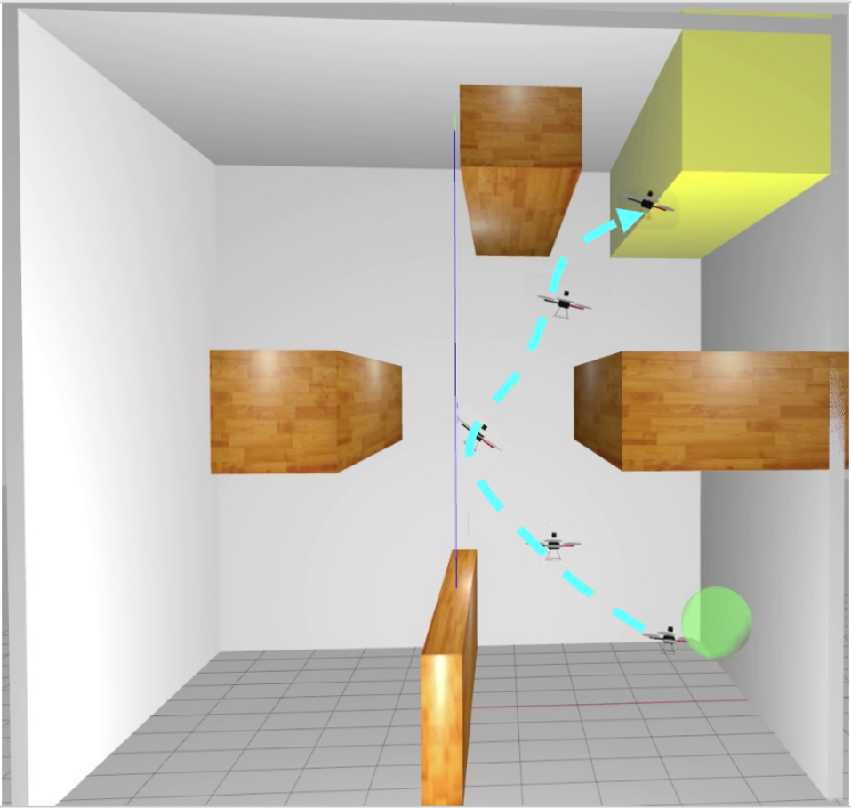
(a) VI-fixed

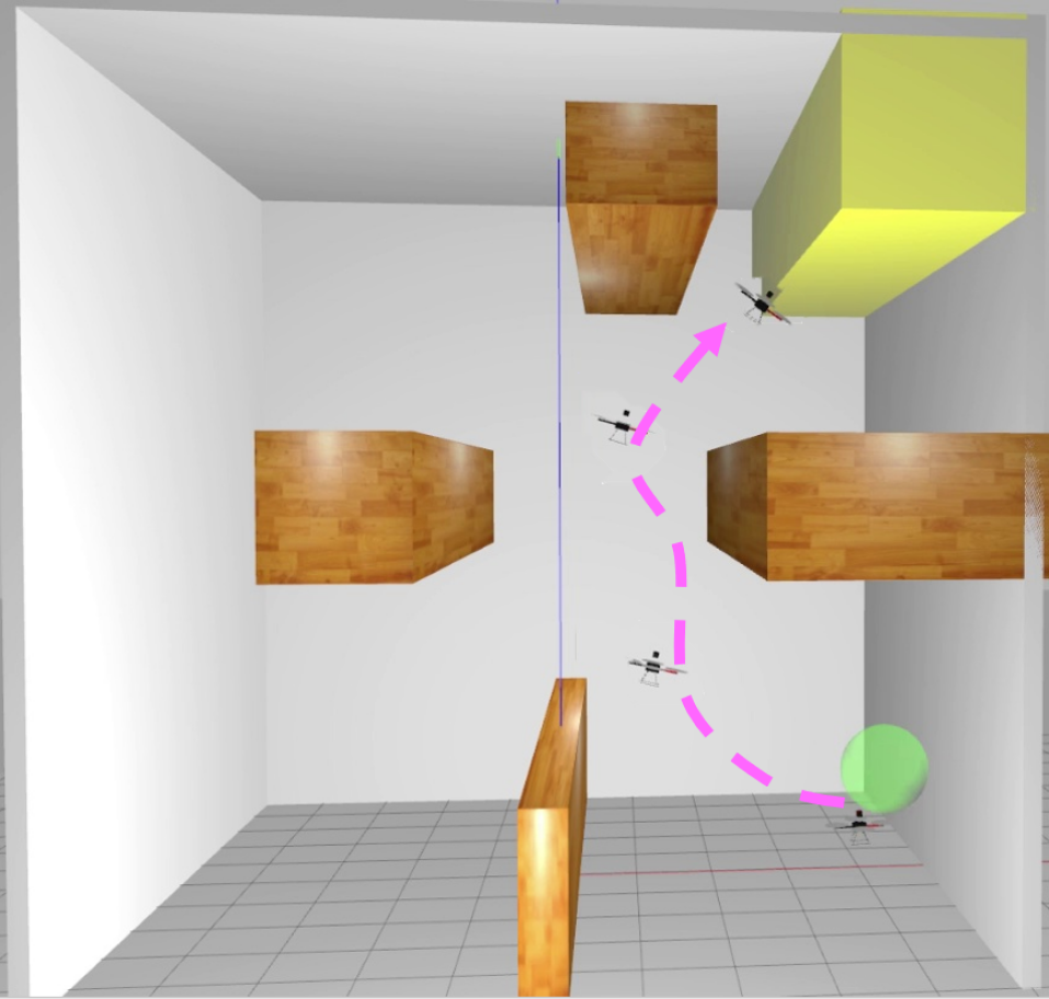
(b) MPC-fixed

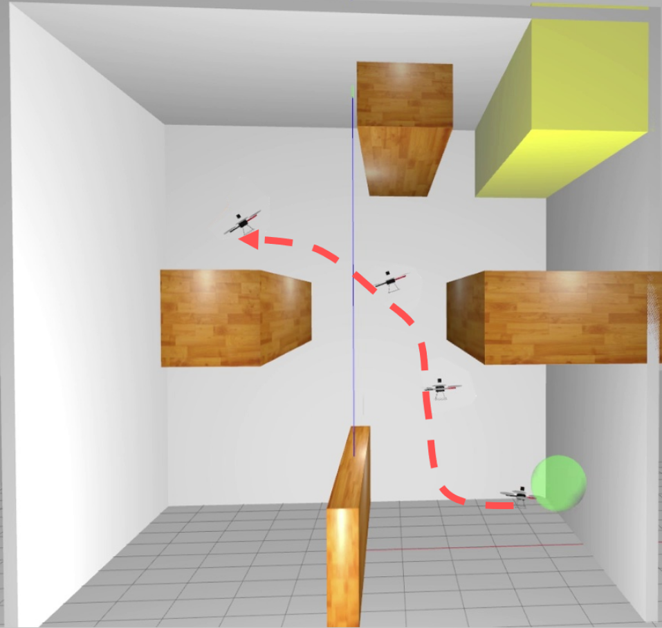
(c) Baseline Approach

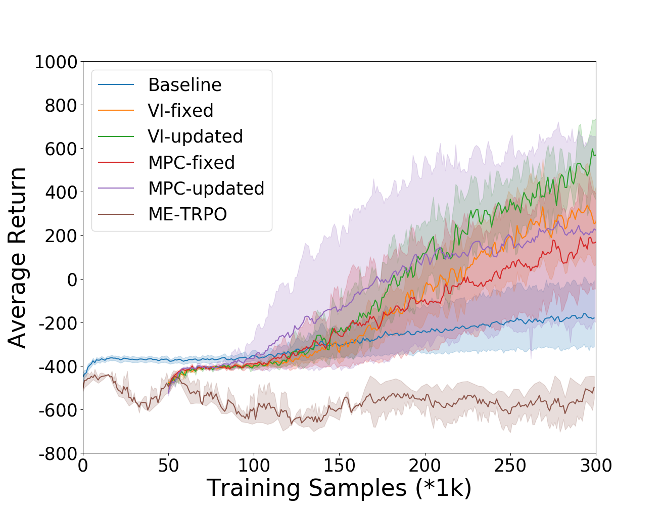
(d) Overall Performance

Figure 2: Simulated quadrotor trajectories from final policies using (a) VI-fixed (b) MPC-fixed and (c) Baseline approach. Our approach learns to fly to the goal yet the baseline approach keeps failing in a undesired (upper-left) area and never recovers. (d) Overall performance comparison on the quadrotor example, with the sample cost at approximately $\mathrm{50K}$ of MBB warm-starting stage included. For both examples, we stop the training at 300K samples as the baseline approach keep failing without any visible progress while MBB approach can reach a success rate over 85% which is sufficient to prove the sample efficiency of our method.

In this section, we show that the MBB approach can be a good alternative to the baseline approach to achieve significant improvement on the RL data efficiency and peak performance, especially under sparse reward.

The baseline approach refers to the model-free PPO update with randomly initialized on-policy value function as baseline $b(s)=V^{\pi}(s)$ and employing regular value update rule, as discussed in Sec. II-B; while the MBB approach refers to the use of same PPO algorithm but with the model-based baseline $b(s)=V^{\mathrm{M}}(s)$ initialized from the value solutions of a simplified, lo-dim problem with an approximate system model, as described in Sec. III. MBB has four variants: VI-fixed, VI-updated, MPC-fixed and MPC-updated, depending on the use of value iteration or MPC. Moreover, “fixed” refers to the baseline function remains unchanged once initialized while “updated” means the baseline function will be updated based on Eq. (9) and Eq. (10). We also include a well-known model-based algorithm ME-TRPO [10], which use an ensemble of models to directly learn a global, hi-dim system model, to show that hi-dim model is often hard to learn and can sometimes reduce performance.

We use Gazebo simulator [31] to build the robotic system and environment for our hi-dim target RL problem that includes sensory input. We include sensory input as part of the state not only to detect obstacles, but to emphasize the MBB approach is characterized to utilize lo-dim solutions to facilitate the learning of hi-dim policy in a model-free way.

We use Eq. (11) as the (sparse) reward function for the two examples in Section IV, where $\mathbf{G}$ refers to the set of goal states, $\mathbf{C}$ the set of collision states and $\mathbf{I}$ the set of other states which involves neither collision nor goal. Note that here $s$ is the full MDP state, which includes both robotic internal states and sensor readings for the target RL problem $\Omega$. Eq. (12) is used in Section V for the Trap-Goal environment. Here, $\mathbf{Tr}$ represents the states in the trap area.

$$\scriptsize r(s)=\begin{cases}0&\;s\in\mathbf{I}\\ +1000&\;s\in\mathbf{G}\\ -400&\;s\in\mathbf{C}\end{cases}$$ (11)

$$\scriptsize r(s)=\begin{cases}0&\;s\in\mathbf{I}\\ +1000&\;s\in\mathbf{G}\\ +100&\;s\in\mathbf{Tr}\\ -400&\;s\in\mathbf{C}\end{cases}$$ (12)

IV-A Differential Drive Car

We first evaluate our approach on a simulated TurtleBot, which resembles a differential drive car [32, 33] navigating in an environment with multiple static obstacles, as shown in Fig. 1. Note that the robot is not aware of the environment in advance, but needs to learn to correspond hi-dim sensory and internal states to proper actions purely from trial and error. The car aims to learn a collision-free control policy to move from a starting area (green area in Fig. 1) to a specific goal area (yellow area in Fig. 1). The state and observation of this example are discussed in Sec. III-A. The car moves by controlling the speed and turn rate. To warm-start the hi-dim RL process using our MBB approach, we select Eq. (5) as a lo-dim, approximate car system in which only considers $(x,y,\theta)$ as state, linear and angular velocity $(v,\omega)$ as control. It is used to generate lo-dim value data via classical methods to initialize model-based baseline function.

Fig. 1(d) shows the learning progresses for different approaches. We take the averaged training return versus iterations as performance measurement. Results are summarized across 10 different trials. The curves show the mean return and the shaded area represents the standard deviation of 10 trials. As evident from Fig. 1(d), baseline approach is struggling in making progress potentially due to insufficient reward feedback. Similarly, ME-TRPO fails to make progress on learning a goal-reaching policy. This is because the transition model of sensory input like Lidar is too difficult to represent even using a set of neural network-based approximators. However, with a simple replacement of baseline function, MBB approach (all variants) can elevate the learning performance significantly and also avoid fitting a hi-dim model, despite sparse-feedback environment.

As the typical final policy behaviours shown in Fig. 1(a), 1(b) and 1(c), our approach can successfully learn collision-free paths despite the collisions in the earlier stage while the baseline approach only learns highly conservative behaviours such as staying around the same area after many failures.

Fig. 1(d) takes the warm-starting stage required by MBB approach into account for a fair comparison of learning efficiency in terms of sample and computational cost. As summarized in Table. I, the car example only requires $\mathrm{10K}$ samples and $5.5\%$ computational time for MBB warm-starting, which is insignificant compared to that of entire RL process, indicating the efficiency of MBB over the baseline approach. The data in Table. I is measured on the hardware: Intel(R) Core(TM) i7-8700K CPU@3.70GHz; RAM 32GB.

In this example, value iteration is shown to be a better technique compared to MPC for MBB approach. This makes sense as value iteration exhausts all possible state combinations of the lo-dim system while MPC produces a finite set of locally optimal trajectories. With both value iteration and MPC, allowing baseline update further improves performance. This is especially true with MPC and indicates the necessity of introducing an appropriate update criterion. Intuitively, keeping a well-initialized baseline function fixed would be advantageous in preventing policy getting stuck in the early stage; however, eventually such fixed baseline may become somewhat detrimental and can prevent further policy improvement. On the other hand, the significance of improvement also depends on the training quality of the baseline. For example, in Fig. 1(d), VI-updated not bringing much performance improvement over VI-fixed is potentially because the baseline function can be ideally trained on data covering the whole lo-dim state space thus it does not experience substantial changes.

Examples	Types	Cost
		Sample	Computation($\%$)
Car	Value Iteration	$\hfil\mathrm{10K}$	5.5
Quadrotor	MPC	$\mathrm{50K}$	29.2

TABLE I: Cost of warm-starting period of the MBB approach on differential car and planar quadrotor examples. Sample cost is measured by the number of timesteps that the agent interacts with the environment during the amount of time needed for warm-starting. Computational cost is represented by the wall time percentage that warm-starting occupies compared to that of total RL training process, under equivalent computing configuration.

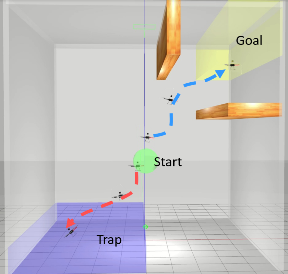
(a) Trap-Goal Environment

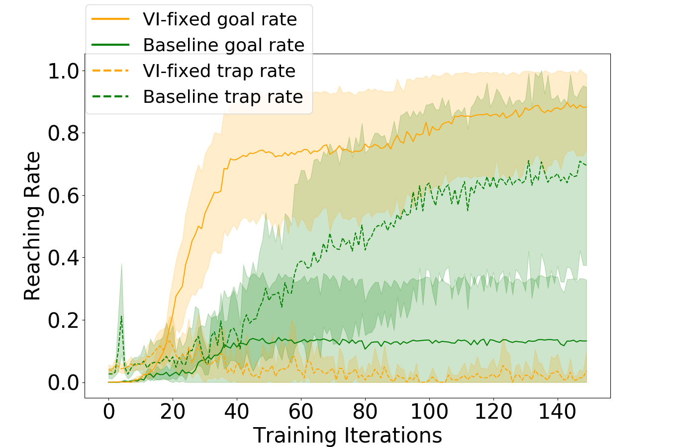
(b) Trap/Goal Reaching Rate

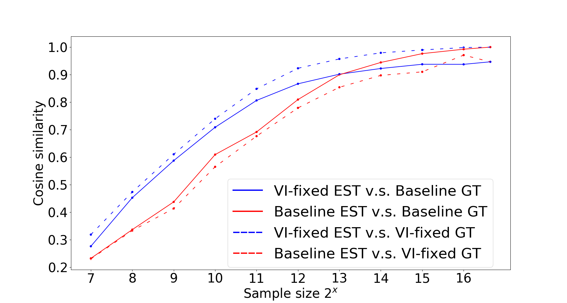
(c) Policy Gradient Correctness

Figure 3: (a) Quadrotor trajectories in the Trap-Goal environment using MBB (blue dashed line) and the baseline approach (red dashed line). (b) The training performance of MBB and the baseline approach in terms of goal and trap reaching rate. (c) The comparison of policy gradient estimation correctness between using MBB and the baseline approach.

IV-B Planar Quadrotor

In the second example, we simulate a planar quadrotor [12, 34] as a more complicated system to test our approach. The control of a quadrotor is usually considered challenging due to its under-actuated nature. Therefore, the goal of this experiment is to validate that our MBB approach still works well even on a highly dynamic and unstable system. “Planar” means the quadrotor is restricted to move in the vertical ($x$-$z$) plane by changing the pitch without affecting the roll and yaw. The simulated setup is shown in Fig. 2, with starting region (green area) and goal region (yellow area).

To use our approach, we choose a 6D system model in Eq. (7) to approximately resemble a planar quadrotor and generate the lo-dim value data for MBB initialization. The internal state is defined as $\mathbf{x}=(x,v_{x},z,v_{z},\psi,\omega)$, where $x,z,\psi$ denote the planar positional coordinates and pitch angle, and $v_{x},v_{z},\omega$ denote their time derivatives respectively. The quadrotor receives full state $s=(x,v_{x},z,v_{z},\psi,\omega,d_{1},...,d_{8})$, which contains eight sensor readings extracted from the laser rangefinder for obstacle detection, in addition to the internal state $x$. The quadrotor intends to learn a policy mapping from states and observations to its two thrusts $F_{1}$ and $F_{2}$ to reach the goal.

Fig. 2(d) depicts the evaluation of the MBB, the baseline as well as the model-based RL approach on the planar quadrotor, in a similar way as the car example. Despite the computational complexity, we still apply value iteration on the 6D approximate state space to fully test our approach on complex systems. The average returns from the four variants of our approach start outperforming the baseline approach at 150 iteration. In contrast with MPC-based technique, value iteration ends up with the best performance and much lower variance, indicating its notable advantage in giving accurate, robust value supervision. However, it is worth noting that the MPC based technique retains more scalability to relatively complex systems without losing too much learning performance. Moreover, although MPC-based warm-starting on the quadrotor requires higher sample and computational cost than the car as shown in Table. I, the overall learning efficiency is still significantly improved.

In terms of ME-TRPO, it struggles in improving the policy due to the difficulty of modelling hi-dim sensory evolution, as shown in Fig. 2(d). As a result, the policy learning gets affected due to the unreliable training data produced by the neural network models. This also reflects the advantage of using our MBB approach in that we do not need to directly learn a hi-dim model.

The trajectories plots also highlight the efficiency of our approach. As evident in Fig. 2(c), the baseline approach fails to find the correct path and gets stuck in an undesirable region. This is potentially because the baseline approach forces its baseline (on-policy value function $V^{\pi}(\cdot)$) to be constantly updated towards policy return, and this can result in near-zero advantage estimation [19] and restrain further policy exploration, which is especially unfavourable to an initially poorly performing policy. In contrast, the variants of our approach can avoid such issue by leveraging approximate model priors to construct model-based baseline $V^{\mathrm{M}}(\cdot)$ and applying proper baseline update criterion. Therefore, our approach tractably and reliably learns a policy that smoothly and successfully reaches the goal.

V Discussion: Policy Gradient Correctness

In this section, we investigate the correctness of policy gradient estimation to gain insight on why our approach is able to improve learning efficiency. More analysis on the policy advantage and gradient variance can be found in [28]. We take VI-fixed as a typical variant of our MBB approach.

To highlight the importance of correct gradient estimation in RL tasks, we purposely design a “Trap-Goal” example shown in Fig. 3(a), which contains a goal (yellow area) and trap (purple area) that give positive but various rewards ($+1000$ for goal, $+100$ for trap) such that the correct policy gradient should drive the policy towards reaching the goal despite possible misleading gradients caused by the trap.

Fig. 3(a) depicts trajectories by executing policies learned from MBB and the baseline approach. Under same exploration strategy, the baseline approach leads to a trap-reaching policy (red dashed line) while MBB approach learns the desired goal-reaching policy (blue dashed line). This result is also reflected in Fig. 3(b) where MBB approach has an increasing goal-reaching rate as learning progresses while the baseline approach has an increasing trap-reaching rate. Combining the results in Fig. 3(a) and Fig. 3(b), we demonstrate that the way the MBB approach helps is by providing global guidance to exploration in model-free RL. In this “Trap-Goal” example, although the “Trap” provides positive reward which should be a good incentive for RL, the lo-dim solutions perceive that the “Goal” region provides even better reward, so that the the policy is optimized towards a globally-optimal direction.

Fig. 3(c) intends to show that the MBB approach provides more favourable policy gradient estimation than baseline approach, by quantifying the closeness between the estimated and true policy gradients which computed by the MBB and the baseline approach respectively. We denote baseline GT and VI-fixed GT as two types of true policy gradients that are obtained by calculating Eq. (1) (using $V^{\pi}$ or $V^{M}$) over infinite samples collected from an initial policy $\pi_{0}$. Correspondingly, with $\mathrm{N}(\mathrm{N}\leq\mathrm{N}_{\max})$ samples, we obtain two types of gradient estimation named baseline EST and VI-fixed EST. By selecting different sample size $\mathrm{N}$ and computing the cosine similarity for four EST/GT combination, we plot the results in Fig. 3(c). The results are averaged over 100 random selections of $\mathrm{N}$ samples. With higher cosine similarity, our MBB approach (blue solid and dashed lines) leads to more accurate gradient estimation than the baseline approach in terms of gradient direction, regardless of sample size or ground truth type, especially at relatively low $\mathrm{N}$.

VI Conclusion and future work

We propose Model-Based Baseline, a novel approach to alleviate the data inefficiency of model-free RL in hi-dim applications by implicitly leveraging model priors from a associated lo-dim problems. This is achieved by first solving a simplified, lo-dim version of the RL problem which allows the use of known, approximate system models to calculate a lo-dim value function using classical methods. The lo-dim value function are then used to warm-start a baseline function, which can act as a useful value priors to provide “global guidance” for the hi-dim model-free RL process. The results show that by providing more accurate policy gradient estimation, our approach can significantly accelerate hi-dim model-free RL.

Our findings open exciting directions for future work. One direct idea is to explore the possibilities of novel warm-starting strategies for both policy and value functions of a hi-dim RL problem from solutions of a lo-dim problem. We are also planning to deploy our approach on a real robot to further validate its robustness and feasibility on real world RL problem.

Appendix

A Data Generation using MPC

A1 General MPC Formulation

The goal of MPC for both examples is to generate trajectories from certain initial states to a desired goal region whilst avoiding obstacles. Using the point-mass optimization-based collision avoidance approach, the obstacle avoidance condition is:

$$\text{dist}(p,\mathbb{O})>d_{min},$$ (13)

where $\text{dist}(p,\mathbb{O}):=\min_{t}\left\{||t||_{2}:(p+t)\cap\mathbb{O}\neq\emptyset\right\}$. Then, $p$ is the position of the point-mass, $d_{min}\geq 0$ is a desired safety margin with the size of real robot taken into account, and $\mathbb{O}$ denotes a polyhedral obstacle which is a convex compact set with non-empty relative interior, represented as

$$\mathbb{O}=\{p\in\mathbb{R}^{n}:Ap\leq b\},$$ (14)

where $A\in\mathbb{R}^{l\times n}$, $b\in\mathbb{R}^{l}$, $l$ is the number of sides of the obstacle (in our example, all obstacles are shaped as cubes) and $n$ is the dimensionality of positional states. Since (13) is non-differentiable, we reformulate the condition into an equivalent differentiable condition: $\text{dist}(p,\mathbb{O})>d_{min}\iff\exists\lambda\geq 0:(Ap-b)^{\top}\lambda>d_{min},\ ||A^{\top}\lambda||_{2}\leq 1,$ where $\lambda$ is the dual variable. We now formulate the general MPC optimization problem as follows:

$$\min_{\bm{\tilde{s}},\bm{\tilde{a}},\bm{\lambda}} \sum_{k=0}^{H-1}\left((p_{k}-p_{ref})^{\top}\gamma^{k+1}Q(p_{k}-p_{ref})+\tilde{a}_{k}^{\top}R\tilde{a}_{k}\right)$$ (15)

$$+(p_{H}-p_{ref})^{\top}\gamma^{H+1}Q(p_{H}-p_{ref})$$

s.t. $$\tilde{s}_{0}=\tilde{s}_{initial}$$

$$\tilde{s}_{k+1}=\tilde{s}_{k}+T_{s}\tilde{f}(\tilde{s}_{k},\tilde{a}_{k}),\quad\tilde{a}_{k}\in\Delta,\quad\forall k\in\left\{0,\ldots,H-1\right\}$$

$$\tilde{s}_{k}\in\tilde{S},\quad\forall k\in\{0,\ldots,H\}$$

$$\tilde{s}_{H}\in\Gamma_{3}$$

$$\lambda_{k}^{(m)}\geq 0,\quad\left(A^{(m)}p_{k}-b^{(m)}\right)^{\top}\lambda_{k}^{(m)}>d_{min},\quad||A^{(m)^{\top}}\lambda_{k}^{(m)}||_{2}\leq 1,$$

$$\forall m\in\{1,\ldots,M\},\quad\forall k\in\{0,\ldots,H\}$$

To match the notations in the main paper, here we employ $\tilde{s}$ and $\tilde{a}$ as the state and action of a low-dimensional model (as in Eq. (7)) used in MPC. Tilde indicates it is an approximate model $\tilde{f}$ in contrast to the full MDP model $f$ of the target RL problem. Specifically, $H$ is the horizon length, $\bm{\tilde{s}}=[\tilde{s}_{0},\ldots,\tilde{s}_{H}]$ is all the states over the horizon, $\bm{\tilde{a}}=[\tilde{a}_{0},\ldots,\tilde{a}_{H-1}]$ is the actions over the horizon, $\bm{\lambda}=[\lambda_{0}^{(1)},\ldots,\lambda_{0}^{(M)},\lambda_{1}^{(1)},\ldots,\lambda_{H}^{(M)}]$ is the dual variables associated with obstacles $\mathbb{O}^{(1)}\ldots\mathbb{O}^{(M)}$ over the horizon, $M$ is the number of obstacles, $\tilde{s}_{k}$ is the states at time $k$, $p_{k}$ is the positional states at time $k$, $p_{ref}$ is the reference position, $\tilde{a}_{k}$ is the control inputs at time step $k$, $\gamma$ is the scaling factor for the position error, $Q$ is the weight matrix for the position error, $R$ is the weight matrix for the control effort, $\tilde{s}_{initial}$ is the initial state, $T_{s}$ is the sampling period, $\tilde{f}$ is the continuous-time system dynamics, $\Delta$ is the collection of possible control inputs, $\tilde{S}$ is the state constraints, $\Gamma_{3}$ is the collection of goal states, and $A^{(m)}\in\mathbb{R}^{l\times n}$ and $b^{(m)}\in\mathbb{R}^{l}$ define the obstacle $\mathbb{O}^{(m)}$ based on (14).

A2 Car Example MPC Formulation

In the car scenario, the continuous-time system dynamics $\tilde{f}$ is:

$$\dot{\tilde{s}}=\tilde{f}(\tilde{s},\tilde{a})=\begin{bmatrix}\dot{x}\\ \dot{y}\\ \dot{\theta}\end{bmatrix}=\begin{bmatrix}v\cos{(\theta)}\\ v\sin{(\theta)}\\ \omega\end{bmatrix}$$ (16)

where $\tilde{s}=[x,y,\theta]^{\top}$ and $\tilde{a}=[v,\omega]^{\top}$. In the optimization problem we have:

$$H=80;\gamma=1.1;T_{s}=0.05;d_{min}=0.277;M=6$$

$$p=[x,y]^{\top};p_{ref}=[3.5,3.5]^{\top}$$

$$Q=\text{diag}([10,10]^{\top});R=\text{diag}([1,1]^{\top})$$

$$\Delta=\{[v,\omega]^{\top}:-2\leq v\leq 2,\ -2\leq\omega\leq 2\}$$

$$\tilde{S}=\{[x,y,\theta]^{\top}:|x|\leq 4.723,|y|\leq 4.723,-\infty\leq\theta\leq\infty\}$$

$$\Gamma_{3}=\{[x,y,\theta]^{\top}:||[x,y]^{\top}-[3.5,3.5]^{\top}||_{2}\leq 1,\cos{(\theta-0.75)}\leq 0.3\}$$

The matrices for specifying obstacles $\mathbb{O}^{(1)}\ldots\mathbb{O}^{(6)}$ are:

$$\small A^{(m)}=\begin{bmatrix}-1&0\\ 1&0\\ 0&-1\\ 0&1\end{bmatrix},\quad\forall m\in\{1,\ldots,M\}$$ (17)

$$\small\begin{split}b^{(1)}=\begin{bmatrix}0.35\\ 0.35\\ 0.35\\ 0.35\end{bmatrix},b^{(2)}&=\begin{bmatrix}-2.65\\ 3.35\\ 1.35\\ -0.65\end{bmatrix},b^{(3)}=\begin{bmatrix}-1.65\\ 2.35\\ -0.65\\ 1.35\end{bmatrix},\\ b^{(4)}=\begin{bmatrix}2.35\\ -1.65\\ 2.35\\ -1.65\end{bmatrix},b^{(5)}&=\begin{bmatrix}0.35\\ 0.35\\ -3.65\\ 4.35\end{bmatrix},b^{(6)}=\begin{bmatrix}3.35\\ -2.65\\ -1.65\\ 2.35\end{bmatrix}.\end{split}$$ (18)

A3 Quadrotor Example MPC Formulation

In the quadrotor scenario, the continuous-time system dynamics $\tilde{f}$ is denoted as Eq. (7). In the optimization problem we have:

$$H=140;\gamma=1.1;T_{s}=0.05;d_{min}=0.1;M=4$$

$$p=[x,z]^{\top};p_{ref}=[4,9]^{\top}$$

$$Q=\text{diag}([10000,10000]^{\top});R=\text{diag}([1,1]^{\top})$$

$$\Delta=\{[M_{1},M_{2}]^{\top}:5\leq M_{1}\leq 11,\ 5\leq M_{2}\leq 11\}$$

$$\tilde{S}=\{[x,v_{x},z,v_{z},\phi,\omega]^{\top}:|x|\leq 4.75,0.25\leq z\leq 9.75,|\phi|\leq\pi/2\}$$

$$\Gamma_{3}=\{[x,z,\phi]:3\leq x\leq 5,8\leq z\leq 10,-\pi/3\leq\phi\leq\pi/3\}$$

In the quadrotor scenario, $A^{(m)}$ is the same as the car scenario in (17). However, $b^{(1)},\ldots,b^{(4)}$ are:

$$\small\begin{split}b^{(1)}&=\begin{bmatrix}3.25\\ -0.75\\ -3.75\\ 6.25\end{bmatrix},\quad b^{(2)}=\begin{bmatrix}1.25\\ 1.25\\ -7.5\\ 9.5\end{bmatrix},\\ b^{(3)}&=\begin{bmatrix}-1.75\\ 5.75\\ -3.75\\ 6.25\end{bmatrix},\quad b^{(4)}=\begin{bmatrix}0.75\\ 0.75\\ 0.5\\ 2.5\end{bmatrix}\text{.}\end{split}$$ (19)

B More results using TD$(\lambda)$ return

As discussed in Sec. III-C, the TD$(\lambda)$ estimation of $G^{\lambda}_{t}$ can include an on-policy value function $V^{\pi}(s_{t})$ if $\lambda\in[0,1)$. However, we demonstrate that our model-based baseline function $V^{\mathrm{M}}(s_{t})$ can not only act as a choice of the baseline function $b(s_{t})$, but also a special, model-based value function for more general TD$(\lambda)$ return to replace $V^{\pi}(s_{t})$. Without the loss of generality, we test the cases where $\lambda=0.95,0.85$.

Fig. 4 illustrates the learning performance on the car and quadrotor examples respectively using our MBB approach with TD$(\lambda)$ return, where $V^{\pi}(\cdot)$ is replaced by $V^{\mathrm{M}}(\cdot)$. We observe similar data efficiency improvements as using Monte-Carlo return in Sec. IV, which indicates the benefits of MBB approach under general TD$(\lambda)$ return despite the potential bias. We also note that as $\lambda$ deceases, the averaged policy performance decreases correspondingly in certain extent. This is potentially a possible negative effect of using $V^{\mathrm{M}}(s_{t})$ for TD$(\lambda)$ estimation. Since $V^{\mathrm{M}}(s_{t})$ is calculated and approximated from a lower-dimensional problem, it introduces more bias than $V^{\pi}$ in $G^{\lambda}$ estimation. As $\lambda$ deceases, such bias becomes more significant and can be more harmful to the learning process as the value function occupies larger proportion in the TD$(\lambda)$ return.

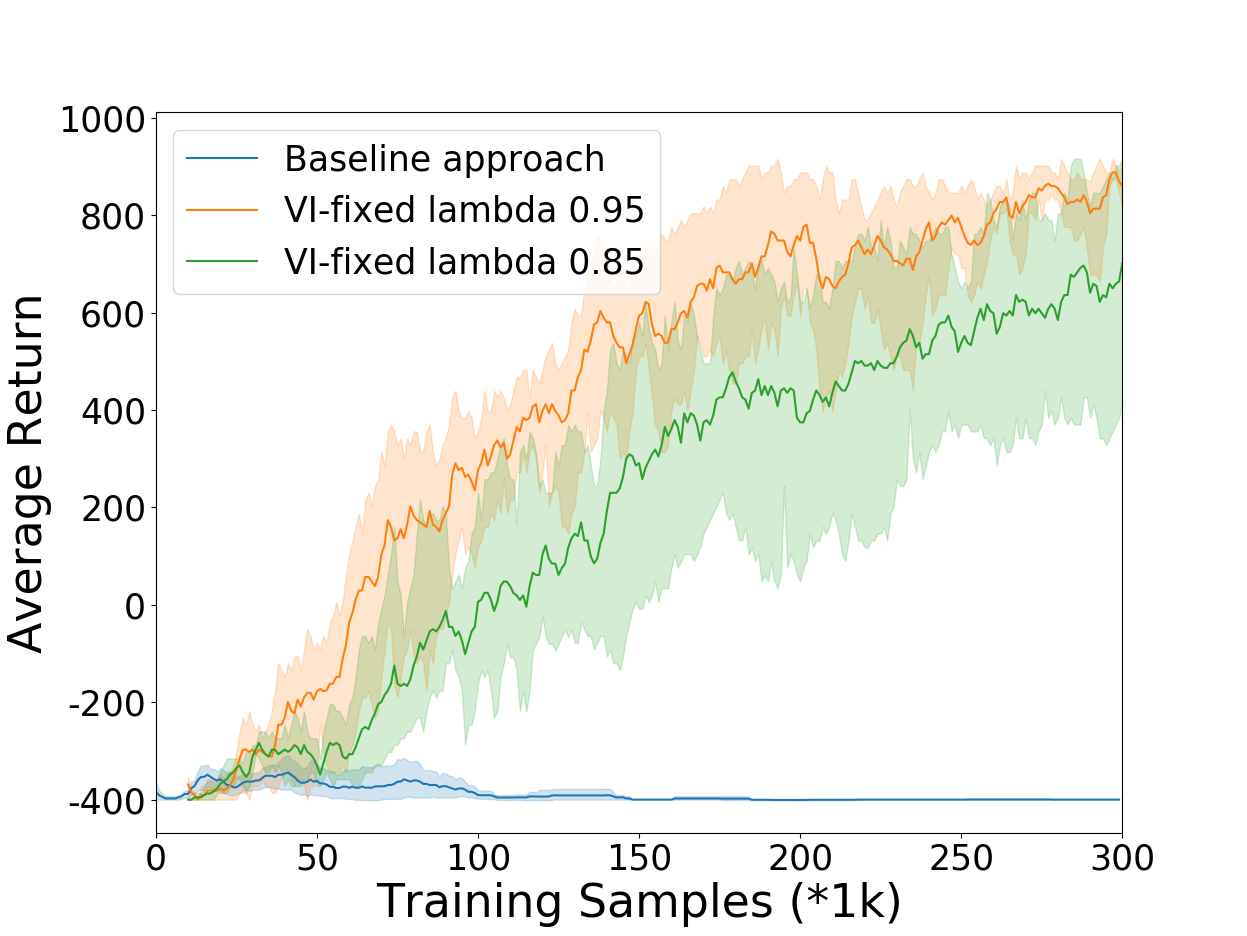
(a) Car example

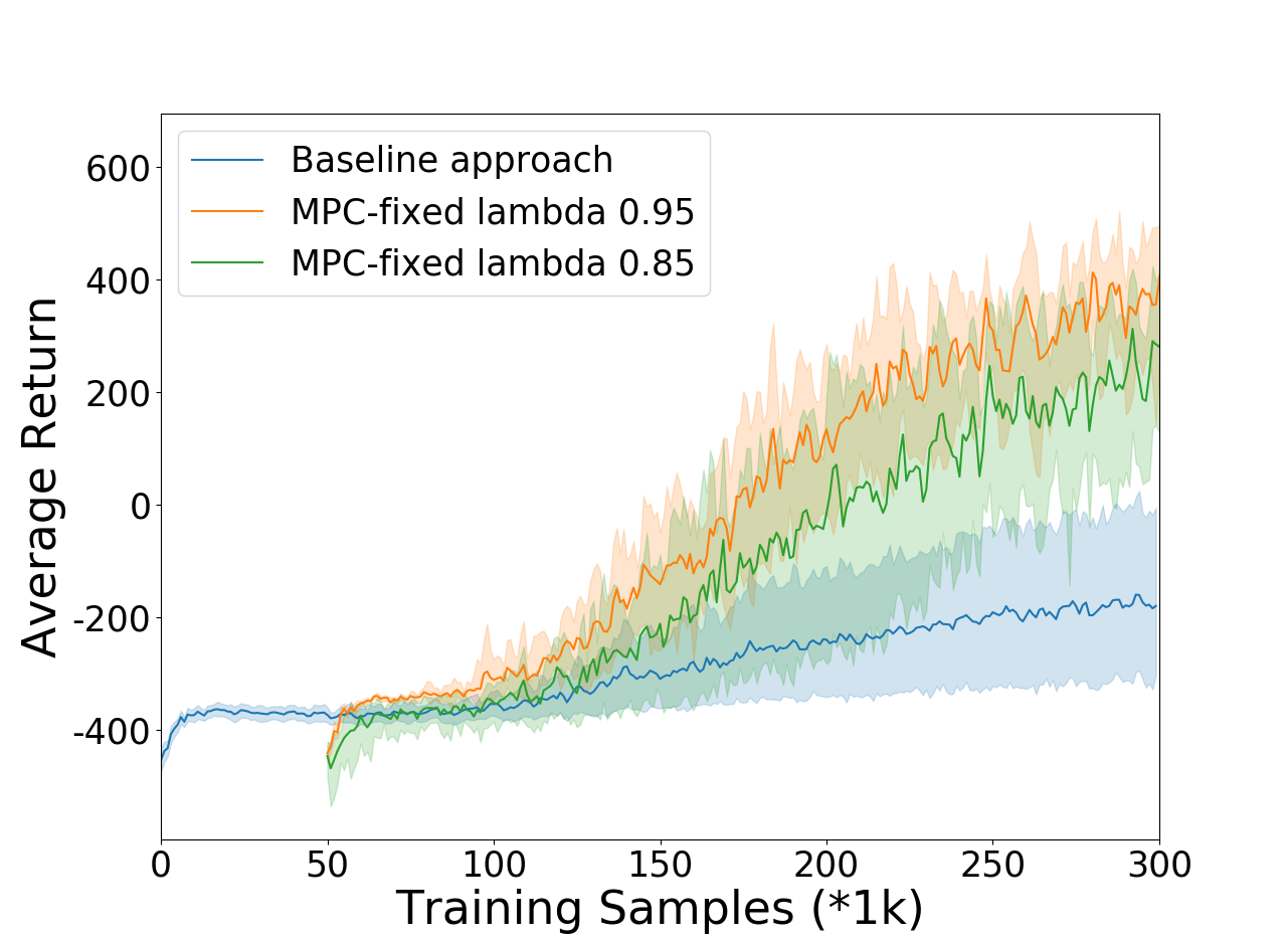
(b) Quadrotor example

Figure 4: Performance comparison between MBB and the baseline approach, where MBB approach uses TD$(\lambda)$ return ($\lambda=0.95,0.85$) for policy gradient calculation.

C More Discussions

C1 Correctness of Policy Gradient Estimation

Following the procedure in Section V, we now further investigate the correctness of gradient estimation in the Trap-Goal environment. We take policies at certain iterations in the earlier learning stage and employ these policies to collect sample transitions from the Trap-Goal environment. Particularly, we denote $\pi_{\small\text{G}}^{20}$, $\pi_{\small\text{G}}^{40}$,$\pi_{\small\text{G}}^{60}$ as polices belong to the goal-reaching trials at iteration 20, 40, 60; $\pi_{\small\text{Tr}}^{20}$, $\pi_{\small\text{Tr}}^{40}$,$\pi_{\small\text{Tr}}^{60}$ as polices belong to the trap-reaching trials at iteration 20, 40, 60.

We first take Fig. 5(a), 5(b) and 5(c) as a group to analyze the results since they are all using trap-reaching polices. In the three sub-figures, MBB approach always provide completely distinct gradient estimation from the baseline approach regardless of sample size or ground truth type (comparing blue, solid line to red, solid line, or blue, dashed line to red, dashed line). This suggests that MBB is capable of distinguishing the wrong policy optimization direction for the Trap-Goal task.

On the other hand, Fig. 5(d), 5(e) and 5(f) show the cosine similarity for different sample sizes with the samples collected from goal-reaching policies. In this case, MBB and the baseline approach have consistent tendencies on gradient estimation. However, even in this case, our MBB approach still provides more accurate gradient estimation than the baseline approach (blue solid and dashed lines are mostly above red solid and dashed lines respectively), especially at relatively lower sample sizes.

(a) $\pi_{\small\text{Tr}}^{20}$

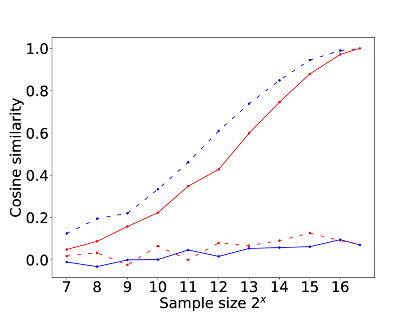
(b) $\pi_{\small\text{Tr}}^{40}$

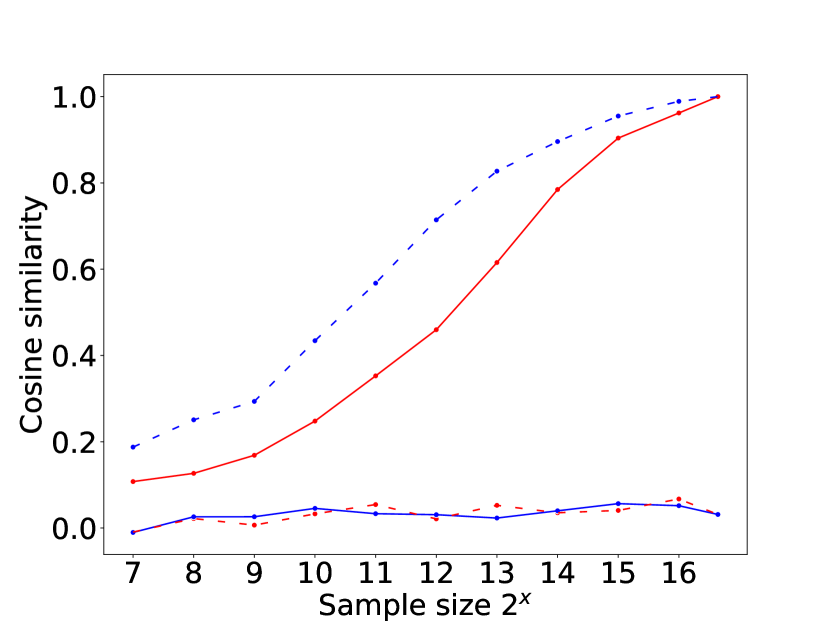
(c) $\pi_{\small\text{Tr}}^{60}$

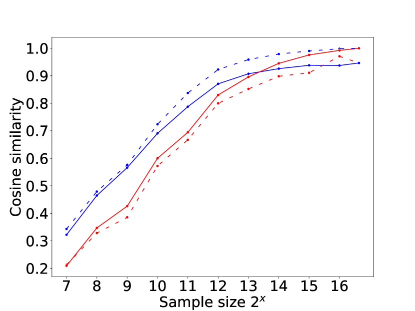
(d) $\pi_{\small\text{G}}^{20}$

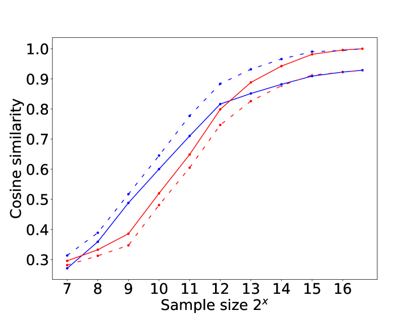
(e) $\pi_{\small\text{G}}^{40}$

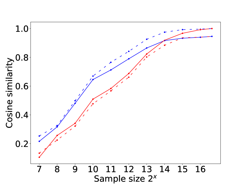
(f) $\pi_{\small\text{G}}^{60}$

Figure 5: The comparison on the correctness of policy gradient estimation between MBB and the baseline approach under varied sampling policies. We take (a), (b), (c) as a group, and (d), (e), (f) as another group to analyze. In each sub-figure, blue lines (solid or dashed) represent MBB-based gradient estimation with regard to different types of ground truths while red lines (solid or dashed) represent that of the baseline approach. A good comparison group would be “blue solid v.s. red solid” or “blue dashed v.s. red dashed”.

C2 Advantage Estimation

We also investigate the advantage estimation to empirically show the efficacy of MBB algorithm. The advantage function $A^{\pi}(s,a)$ measures how much better an action $a$ is than others on average, and has been extensively used in policy gradient algorithms to drive the policy update [19]. In this paper, we assume the advantage is defined by $A^{\pi}(s,a)=G_{t}^{\lambda}-b(s_{t})$ as shown in Eq. (1) where $b(s_{t})$ can be the on-policy value function $V^{\pi}(s_{t})$ or our model-based baseline function $V^{\mathrm{M}}(s_{t})$.

Fig. 6(a) shows the advantage estimation comparison between MBB and the baseline approach. The total number of training iterations are 150 and we take an average of advantage estimation every 10 iterations. It is clearly observed that MBB approach maintains a relatively larger range of advantage estimation over the entire learning process. In contrast, the advantage estimation of the baseline approach gradually shrink to a very narrow range around zero. This may indicate that MBB involves more exploration thus more likely to escape local optima. On the other hand, as we already observed in the Fig. 1(c), the baseline approach can often drive the robot get stuck in an undesired area for a long time due to the negligible advantage estimation.

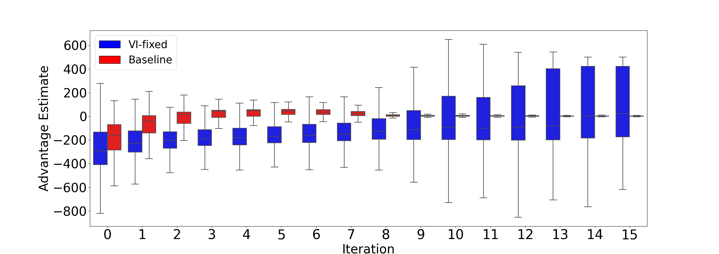
(a) Advantage Estimation

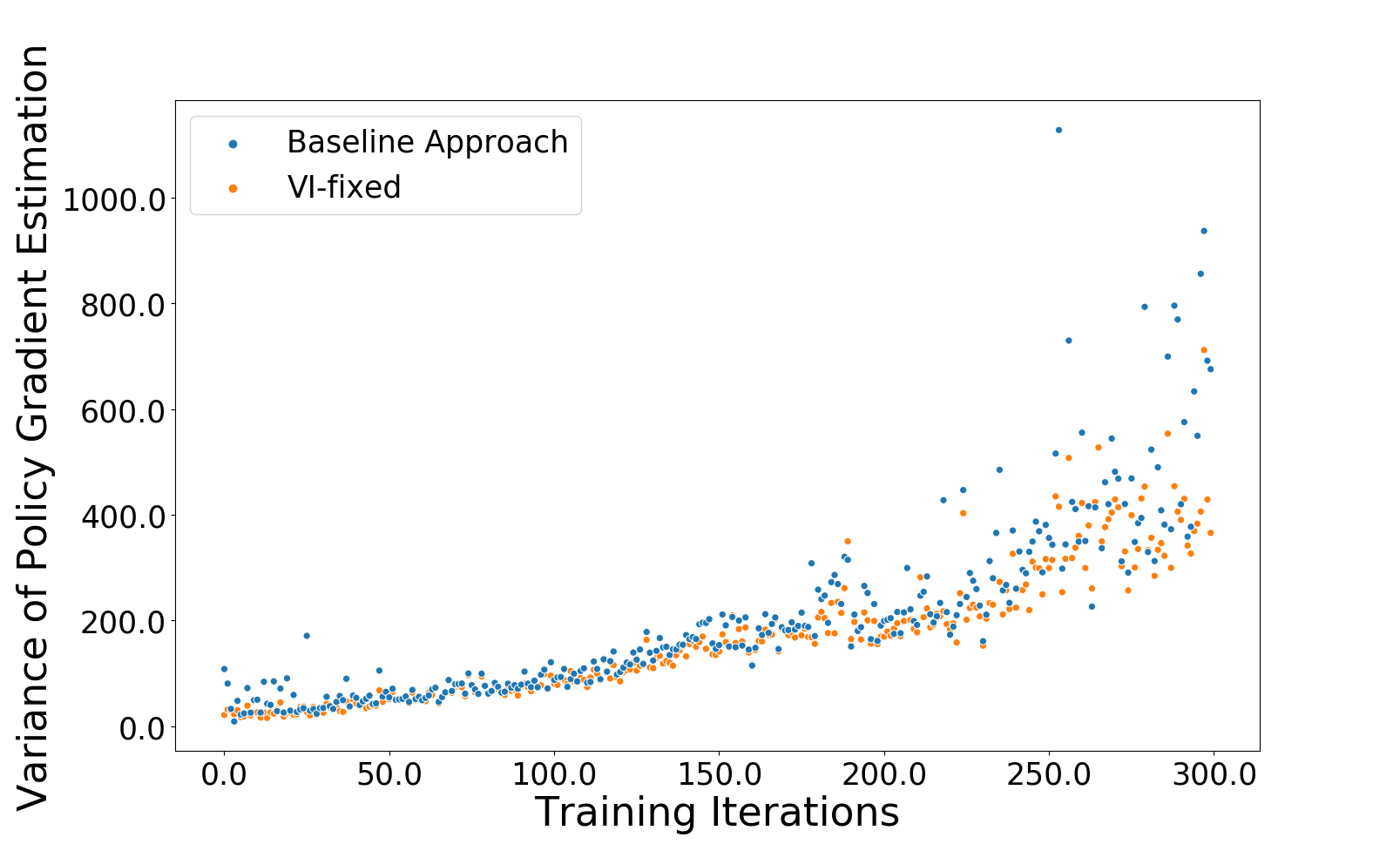
(b) Variance of Policy Gradient Estimation

Figure 6: (a) Advantage estimation versus training iterations using MBB and the baseline approach. Larger colored box refers to wider range of advantage estimation. (b) Policy gradient variance computed via MBB and the baseline approach. Each dot corresponds to the magnitude of variance at certain iteration.

C3 Variance of Policy Gradient Estimation

We also conduct empirical analysis on the variance of gradient estimation. More specifically, at each training iteration, we collect $K$ samples with each of them denoted as $D_{i}=(s_{i},a_{i},r_{i},s_{i+1});i\in\{0,1,2,...,K\}$ using MBB and the baseline approach respectively and calculate $K$ policy gradients $\nabla_{\theta}J(\theta|D_{i})$ based on each sample. Then we compute the largest singular value of co-variance matrix of each set of gradients $\{\nabla_{\theta}J(\theta|D_{i})\;|\;i\in\{0,1,...,K-1\}\}$.

Fig. 6(b) shows the gradient variance magnitude versus training iterations. MBB (orange dots) and the baseline (blue dots) approach share comparable variance of gradient estimation over the entire training process. This fully shows the benefits of our MBB approach since our model-based baseline are facilitating the learning performance by providing necessary exploration and better gradient direction whilst not introducing too much variance.

D Results on Q-learning based Algorithm

In contrast to direct policy gradient based methods (like PPO), Q-learning based methods are another important type of model-free RL algorithms. Deep Deterministic Policy Gradient (DDPG) algorithm is a well-known example. Unlike PPO which directly executes policy gradient optimization, DDPG first learns an on-policy $Q$ function $Q^{\pi}(s,a)$ and then derives a policy based on $Q^{\pi}(s,a)$ [35].

We test our MBB approach on a refined DDPG algorithm (known as TD3 [36]) to demonstrate its compatibility and efficacy on different types of model-free RL algorithms.

D1 Important Procedure of DDPG Algorithm

In DDPG, the $Q$ function $Q^{\pi}(s,a)$ is often represented by a nonlinear function approximator (e.g. neural network) with parameters $\phi$, denoted as $Q^{\pi}_{\phi}(s,a)$. Here we simplify $Q^{\pi}_{\phi}(s,a)$ to $Q_{\phi}(s,a)$ for conciseness. In addition, a $Q$ target function $Q_{\phi_{\operatorname{targ}}}(s,a)$ is introduced in order to alleviate the optimization instability [35]. At each iteration, the $Q$ target function $Q_{\phi_{\operatorname{targ}}}(s,a)$ is also responsible for providing the $Q$ function approximation target $y\left(r,s^{\prime},d\right)$:

$$y\left(r,s^{\prime},d\right)=r(s)+\gamma(1-d)Q_{\phi_{\text{targ}}}\left(s^{\prime},\mu_{\theta_{\text{targ}}}\left(s^{\prime}\right)\right)$$ (20)

where $\mu_{\theta_{\operatorname{targ}}}$ is the parameterized target policy. Then $Q$ function $Q_{\phi}(s,a)$ is updated towards $y\left(r,s^{\prime},d\right)$ by one-step gradient descent using Eq. (21) where $\mathcal{B}$ is a batch of transition data sampled from original RL problem $\Omega$:

$$\phi\leftarrow\phi-\alpha\nabla_{\phi}\frac{1}{|\mathcal{B}|}\sum_{\left(s,a,r,s^{\prime},d\right)\in\mathcal{B}}\left(Q_{\phi}(s,a)-y\left(r,s^{\prime},d\right)\right)^{2}$$ (21)

The policy $\mu_{\theta}$ is updated subsequently via one-step gradient ascent towards $Q_{\phi}(s,a)$ via:

$$\theta\leftarrow\theta+\beta\nabla_{\theta}\frac{1}{|\mathcal{B}|}\sum_{s\in\mathcal{B}}Q_{\phi}\left(s,\mu_{\theta}(s)\right)$$ (22)

$\alpha$ and $\beta$ are step sizes. The $Q$ target $Q_{\phi_{\operatorname{targ}}}(s,a)$ and policy target $\mu_{\theta_{\operatorname{targ}}}$ then need to be updated in certain way such as polyak averaging:

$$\begin{array}[]{l}\phi_{\text{targ }}\leftarrow\rho\phi_{\text{targ }}+(1-\rho)\phi\\ \theta_{\text{targ }}\leftarrow\rho\theta_{\text{targ }}+(1-\rho)\theta\end{array}$$ (23)

D2 MBB-based DDPG Algorithm

We take “VI-fixed” as the representative variant of our MBB algorithm and integrate it into DDPG via the following two steps:

1. Our model-based baseline function $V^{\mathrm{M}}(\cdot)$ can be considered as a special value function which contains the model information from a simplified, low-dimensional problem. Therefore, we can use $V^{\mathrm{M}}(\cdot)$ and one-step simulation to replace $Q_{\phi_{\operatorname{targ}}}(s,a)$ in Eq. (20), where the one-step simulation is shown as Eq. (24) assuming a deterministic full MDP model.

   $$Q_{\phi_{\operatorname{targ}}}(s,a)=r(s)+\gamma V^{\mathrm{M}}(s^{\prime})$$ (24)

2. The variant “VI-fixed” does not enable the subsequent update of $V^{\mathrm{M}}(\cdot)$. Correspondingly, we can disable the update of $Q_{\phi_{\operatorname{targ}}}(s,a)$ in Eq. (23).

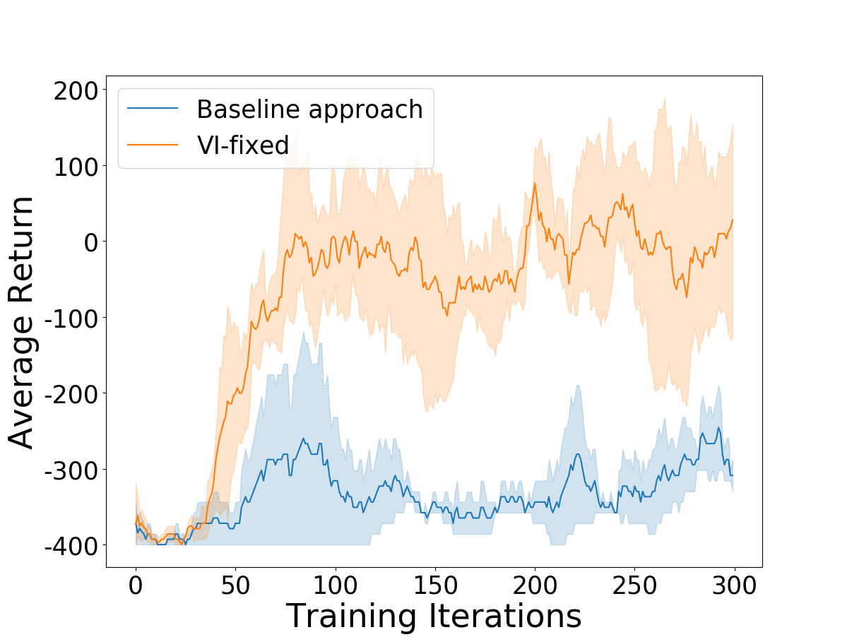
(a) Car Example

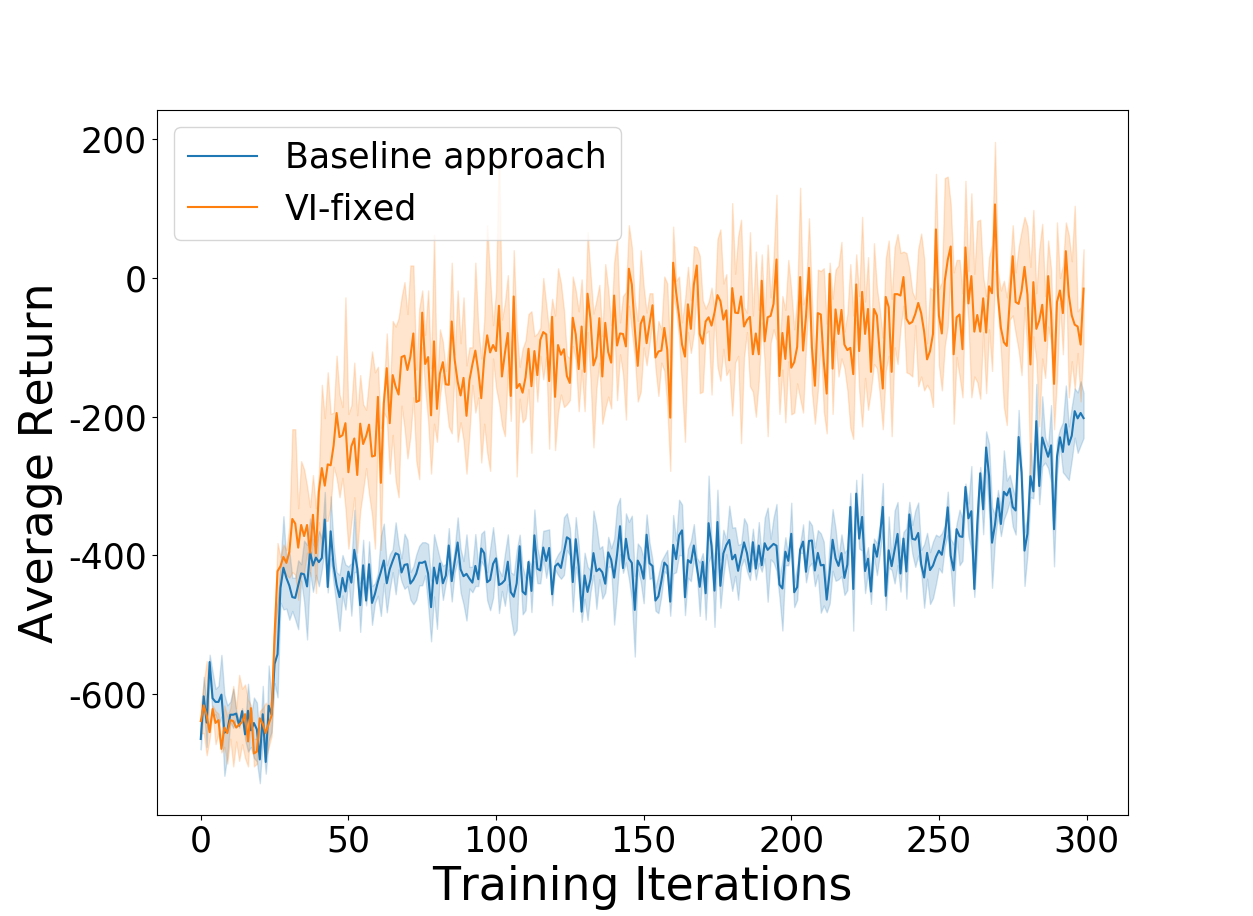
(b) Quadrotor Example

Figure 7: Overall learning performance comparison using MBB-based and the original TD3 algorithms on two robotic examples. We take the averaged training return versus training iterations as performance measurement. Results are summarized across 5 different trials. The curves show the mean return and the shaded area represents the standard deviation of 5 trials.

Particularly in TD3 algorithm, there are two $Q$ target functions: $Q_{\phi_{\operatorname{targ,1}}}(s,a)$ and $Q_{\phi_{\operatorname{targ,2}}}(s,a)$, and $y\left(r,s^{\prime},d\right)$ is computed by:

$$y\left(r,s^{\prime},d\right)=r(s)+\gamma(1-d)\min_{i=1,2}Q_{\phi_{\text{targ },i}}\left(s^{\prime},a^{\prime}\left(s^{\prime}\right)\right)$$ (25)

Therefore, with MBB, we simply use $V^{\mathrm{M}}(\cdot)$ and Eq. (24) to replace both $Q$ target functions $Q_{\phi_{\operatorname{targ,1}}}(s,a)$ and $Q_{\phi_{\operatorname{targ,2}}}(s,a)$ and disable the update of them.

Fig. 7 illustrates how the learning progresses with MBB-based and the original TD3 algorithm (noted as the baseline approach) on two robotic problems in Section IV. Note that the baseline approach uses random initialized $Q$ target function and regular $Q$ target update following Eq. (23). MBB approach refers to a new TD3 algorithm that involves the refinement described in this section. As evident from Fig. 7, MBB approach continues to improve the policy with tolerable variance, and outperforms the baseline approach at around 50 iterations on both examples. For the quadrotor case, even though the baseline approach eventually improves at around 280 iteration, it largely lags behind MBB approach and shows poor data efficiency.

E Code base and hyper-parameters of neural networks

For the PPO algorithm, we follow the implementations from OpenAI Baselines [37]. For the TD3 algorithm, we follow the original implementations from the author. Table. II summarizes the neural network structure as well as the main hyper-parameters of PPO and TD3 algorithm.

	PPO	TD3
Type of layers	FC	FC
Structure of layers	(64,64)	(256,256)
Total timesteps	300K	300K
Policy clipping	0.2	$\times$
Learning rate	$3e^{-4}$	$1e^{-3}$
SGD Optimizer	Adam	Adam
Discount $\gamma$	0.998	0.99
$\lambda$ for TD$(\lambda)$ return	[1, 0.95, 0.85]	$\times$
Gradient clipping	0.5	$\times$
Policy noise	$\times$	0.2
Policy update frequency	$\times$	2
Target network update rate	$\times$	0.005

TABLE II: Main hyper-parameters and neural network structures for PPO and TD3 algorithm.

References

- [1] R. S. Sutton, D. A. McAllester, S. P. Singh, and Y. Mansour, “Policy gradient methods for reinforcement learning with function approximation,” in Advances in neural information processing systems, 2000, pp. 1057–1063.
- [2] A. Bemporad, M. Morari, V. Dua, and E. N. Pistikopoulos, “The explicit linear quadratic regulator for constrained systems,” Automatica, vol. 38, no. 1, pp. 3–20, 2002.
- [3] V. Mnih, K. Kavukcuoglu, D. Silver, A. Graves, I. Antonoglou, D. Wierstra, and M. Riedmiller, “Playing atari with deep reinforcement learning,” arXiv preprint arXiv:1312.5602, 2013.
- [4] N. O. Lambert, D. S. Drew, J. Yaconelli, S. Levine, R. Calandra, and K. S. Pister, “Low-level control of a quadrotor with deep model-based reinforcement learning,” IEEE Robotics and Automation Letters, vol. 4, no. 4, pp. 4224–4230, 2019.
- [5] J. Schulman, S. Levine, P. Abbeel, M. Jordan, and P. Moritz, “Trust region policy optimization,” in International conference on machine learning, 2015, pp. 1889–1897.
- [6] M. Chen and C. J. Tomlin, “Hamilton–jacobi reachability: Some recent theoretical advances and applications in unmanned airspace management,” Annual Review of Control, Robotics, and Autonomous Systems, vol. 1, pp. 333–358, 2018.
- [7] M. Chen, J. F. Fisac, S. Sastry, and C. J. Tomlin, “Safe sequential path planning of multi-vehicle systems via double-obstacle hamilton-jacobi-isaacs variational inequality,” in 2015 European Control Conference (ECC). IEEE, 2015, pp. 3304–3309.
- [8] M. Chen, J. C. Shih, and C. J. Tomlin, “Multi-vehicle collision avoidance via hamilton-jacobi reachability and mixed integer programming,” in 2016 IEEE 55th Conference on Decision and Control (CDC). IEEE, 2016, pp. 1695–1700.
- [9] A. Nagabandi, G. Kahn, R. S. Fearing, and S. Levine, “Neural network dynamics for model-based deep reinforcement learning with model-free fine-tuning,” 2018 IEEE International Conference on Robotics and Automation (ICRA), pp. 7559–7566, 2018.
- [10] T. Kurutach, I. Clavera, Y. Duan, A. Tamar, and P. Abbeel, “Model-ensemble trust-region policy optimization,” in International Conference on Learning Representations, 2018. [Online]. Available: https://openreview.net/forum?id=SJJinbWRZ
- [11] A. Balluchi, A. Bicchi, A. Balestrino, and G. Casalino, “Path tracking control for dubin’s cars,” in Proceedings of IEEE International Conference on Robotics and Automation, vol. 4. IEEE, 1996, pp. 3123–3128.
- [12] G. Wu and K. Sreenath, “Safety-critical control of a planar quadrotor,” in 2016 American Control Conference (ACC). IEEE, 2016, pp. 2252–2258.
- [13] M. P. Deisenroth and C. E. Rasmussen, “Reducing model bias in reinforcement learning,” 2010.
- [14] E. Langlois, S. Zhang, G. Zhang, P. Abbeel, and J. Ba, “Benchmarking model-based reinforcement learning,” arXiv preprint arXiv:1907.02057, 2019.
- [15] J. Chemali and A. Lazaric, “Direct policy iteration with demonstrations,” in Twenty-Fourth International Joint Conference on Artificial Intelligence, 2015.
- [16] J. Kober, K. Mülling, O. Krömer, C. H. Lampert, B. Schölkopf, and J. Peters, “Movement templates for learning of hitting and batting,” in 2010 IEEE International Conference on Robotics and Automation. IEEE, 2010, pp. 853–858.
- [17] S. Levine and V. Koltun, “Guided policy search,” in International conference on machine learning. PMLR, 2013, pp. 1–9.
- [18] T. Zhang, G. Kahn, S. Levine, and P. Abbeel, “Learning deep control policies for autonomous aerial vehicles with mpc-guided policy search,” in 2016 IEEE international conference on robotics and automation (ICRA). IEEE, 2016, pp. 528–535.
- [19] J. Schulman, P. Moritz, S. Levine, M. I. Jordan, and P. Abbeel, “High-dimensional continuous control using generalized advantage estimation,” CoRR, vol. abs/1506.02438, 2016.
- [20] R. S. Sutton, “Learning to predict by the methods of temporal differences,” Machine learning, vol. 3, no. 1, pp. 9–44, 1988.
- [21] E. Greensmith, P. L. Bartlett, and J. Baxter, “Variance reduction techniques for gradient estimates in reinforcement learning,” Journal of Machine Learning Research, vol. 5, no. Nov, pp. 1471–1530, 2004.
- [22] R. Bellman, “Dynamic programming and stochastic control processes,” Information and control, vol. 1, no. 3, pp. 228–239, 1958.
- [23] N. Cesa-Bianchi, C. Gentile, G. Lugosi, and G. Neu, “Boltzmann exploration done right,” in Proceedings of the 31st International Conference on Neural Information Processing Systems, ser. NIPS’17. Red Hook, NY, USA: Curran Associates Inc., 2017, p. 6287–6296.
- [24] Y. Pu, M. N. Zeilinger, and C. N. Jones, “Inexact fast alternating minimization algorithm for distributed model predictive control,” in 53rd IEEE Conference on Decision and Control, 2014, pp. 5915–5921.
- [25] H. Hu, Y. Pu, M. Chen, and C. J. Tomlin, “Plug and play distributed model predictive control for heavy duty vehicle platooning and interaction with passenger vehicles,” in 2018 IEEE Conference on Decision and Control (CDC), 2018, pp. 2803–2809.
- [26] X. Zhang, A. Liniger, and F. Borrelli, “Optimization-based collision avoidance,” IEEE Transactions on Control Systems Technology, 2020.
- [27] M. Chen, S. L. Herbert, H. Hu, Y. Pu, J. F. Fisac, S. Bansal, S. Han, and C. J. Tomlin, “Fastrack: a modular framework for real-time motion planning and guaranteed safe tracking,” 2021.
- [28] X. Lyu, S. Li, S. Siriya, M. Chen, and Y. Pu, “Appendix of mbb: Model-based baseline for global guidance of model-free reinforcement learning via lower-dimensional solutions.” [Online]. Available: https://github.com/SFU-MARS/mbb/blob/master/xlv_MBB_appendix.pdf
- [29] B. Ivanovic, J. Harrison, A. Sharma, M. Chen, and M. Pavone, “Barc: Backward reachability curriculum for robotic reinforcement learning,” in Proc. IEEE Int. Conf. Robotics and Automation, 2019.
- [30] A. Wächter and L. T. Biegler, “On the implementation of an interior-point filter line-search algorithm for large-scale nonlinear programming,” Mathematical Programming, vol. 106, no. 1, pp. 25–57, apr 2005. [Online]. Available: https://doi.org/10.1007%2Fs10107-004-0559-y
- [31] N. Koenig and A. Howard, “Design and use paradigms for gazebo, an open-source multi-robot simulator,” in IEEE/RSJ International Conference on Intelligent Robots and Systems, Sendai, Japan, Sep 2004, pp. 2149–2154.
- [32] S. Bhattacharya, R. Murrieta-Cid, and S. Hutchinson, “Optimal paths for landmark-based navigation by differential-drive vehicles with field-of-view constraints,” IEEE Transactions on Robotics, vol. 23, no. 1, pp. 47–59, 2007.
- [33] M. Al-Sagban and R. Dhaouadi, “Neural-based navigation of a differential-drive mobile robot,” in 2012 12th International Conference on Control Automation Robotics & Vision (ICARCV). IEEE, 2012, pp. 353–358.
- [34] T. Tomić, M. Maier, and S. Haddadin, “Learning quadrotor maneuvers from optimal control and generalizing in real-time,” in 2014 IEEE International Conference on Robotics and Automation (ICRA). IEEE, 2014, pp. 1747–1754.
- [35] T. P. Lillicrap, J. J. Hunt, A. Pritzel, N. M. O. Heess, T. Erez, Y. Tassa, D. Silver, and D. Wierstra, “Continuous control with deep reinforcement learning,” CoRR, vol. abs/1509.02971, 2016.
- [36] S. Fujimoto, H. Van Hoof, and D. Meger, “Addressing function approximation error in actor-critic methods,” arXiv preprint arXiv:1802.09477, 2018.
- [37] P. Dhariwal, C. Hesse, O. Klimov, A. Nichol, M. Plappert, A. Radford, J. Schulman, S. Sidor, Y. Wu, and P. Zhokhov, “Openai baselines: high-quality implementations of reinforcement learning algorithms,” 2019.