Ice stream formation

Abstract

Ice streams are bands of fast-flowing ice in ice sheets. We investigate their formation as an example of spontaneous pattern formation, based on positive feedbacks between dissipation and basal sliding. Our focus is on temperature-dependent subtemperate sliding, where faster sliding leads to enhanced dissipation and hence warmer temperatures, weakening the bed further, although we also treat a hydromechanical feedback mechanism that operates on fully molten beds. We develop a novel thermomechanical model capturing ice-thickness scale physics in the lateral direction while assuming the the flow is shallow in the main downstream direction. Using that model, we show that formation of a steady-in-time pattern can occur by the amplification in the downstream direction of noisy basal conditions, and often leads to the establishment of a clearly-defined ice stream separated from slowly-flowing, cold-based ice ridges by narrow shear margins, with the ice stream widening in the downstream direction. We are able to show that downward advection of cold ice is the primary stabilizing mechanism, and give an approximate, analytical criterion for pattern formation.

1 Introduction

Ice streams are narrow bands of fast flow within otherwise more slowly-flowing ice sheets, often forming near the margin or grounding line of the ice sheet as outlets that can carry the majority of the ice discharged [1]. Some ice streams are confined to topographic lows that channelize flow [2], but not all, and those that are not controlled by topography may occur in parallel arrays of roughly similar ice streams. Where bed topography is not the primary control, several positive feedback mechanisms have been suggested for the formation of an alternating pattern of fast and slow flow.

The viscosity of ice is temperature-dependent, and as a result there is a natural positive feedback between dissipation, reduced viscosity, and faster flow, studied in detail in [3] and likely the cause of often pathological pattern formation in early thermomechanical ice sheet simulations (in the sense of grid-dependent results with no evidence of a short-wavelength cut-off, see [4]). An alternative view holds that ice streams form as the result of high water pressure (or more precisely, lower effective pressure, the difference between normal stress and water pressure) at the ice sheet bed. This can cause pattern formation through a hydromechanical positive feedback in which a reduced effective pressure leads to faster sliding and more water production, which in turn requires effective pressure to be decreased further in order to open basal drainage conduits to evacuate that water [5, 6, 7].

Situated somewhere between these two extremes is the possibility that sliding can occur at the ice sheet bed before the melting point has been reached, and there is no liquid water. Friction generated by this type of subtemperate sliding can be expected to be temperature-dependent [8, 9], leading to a potential positive feedback between raised temperature, faster flow, and enhanced dissipation of heat. This has been studied previously by [10], though using a simplified model and ostensibly as a way of emulating the dissipation-viscosity feedback described above.

Motivated by recent work [11] that demonstrates that subtemperate sliding must happen somewhere in the transition between a cold-based ice sheet that essentially does not slide, and a warm-based ice sheet sliding over a bed at the melting point, we revisit the pattern formation due to subtemperate sliding here. That said, our model turns out to be equally applicable to the hydromechanical patterning process described above.

The paper is organized as follows: first, we develop a novel model that combines thin-film balances in the main along-flow direction with the full mechanics and thermal physics relevant to lateral length scales comparable to ice thickness (§2). This turns out to be key to capturing negative feedbacks that stabilize short wavelengths during pattern formation, and to allowing fully formed ice streams to emerge with a sharp lateral margin (henceforth, ‘margin’) between the ice stream and the surrounding, slowly flowing ice ridge. In that sense, the model is the minimal model that allows these features to form self-consistently.

In order to isolate the basal dissipation feedback, we make ice viscosity independent of temperature. In fact, we use a constant viscosity model. Incorporating a temperature- and strain-rate-dependent viscosity like Glen’s law [12] into the model in future is straightforward in principle. Next, we look for steady state solutions of the model (§33.1), whose form allows unique solutions to be found by simple forward integration from a central ice divide [13, 14]. We show numerically that small perturbations of basal properties can become amplified in the downstream direction, but that this need not happen, and that it can occur in two flavours: the dissipation-temperature feedback in the region of subtemperate sliding, and, in the absence of the former, the hydromechanical feedback for temperate beds (§§33.3–3.5).

Next, we determine analytically a criterion for steady-state patterning to occur during subtemperate sliding (§4), with additional results regarding hydromechanical patterning confined to the supplementary material. We conclude by putting our results in the context of the existing literature (§5) and identifying pressing areas for future research (§6). For a broader overview of the literature on ice stream modelling in the context of ice sheet simulations, we refer the interested reader to the introduction to [11].

2 Model Formulation

We use a dimensionless curvilinear coordinate system $(x,y,z)$ in which the $z$-axis is oriented vertically, $x$ is oriented in the mean flow direction and $y$ is transverse to the mean flow direction. For any fixed $x$, $z=0$ corresponds to the elevation of the bed, which we assume to be a given function of the downstream coordinate $x$ only (a model extension to beds with lateral variation is possible but not useful as a first step). The implied curvature of the coordinate system will turn out not to matter since the radius of curvature is comparable with the length of the ice sheet and curvature terms therefore scale as the ice sheet aspect ratio $\varepsilon$. The coordinates $(y,z)$ describing position the in plane transverse to the main flow direction are scaled with a typical ice thickness scale, and (despite the curvilinear nature of the coordinate system), the $(y,z)$-coordinate system is Cartesian for fixed $x$. The along-flow coordinate is scaled with the length of the ice sheet.

Let $\nabla_{\perp}=({\partial}/{\partial y},{\partial}/{\partial z})$ be the gradient operator in the $(y,z)$-plane. Correspondingly, define $\mbox{\boldmath$v$}_{\perp}=(v,w)$ as a transverse velocity field, scaled by the usual shearing velocity scale [15] multiplied by the ice sheet aspect ratio $\varepsilon$, while $u$ is the component of velocity in the main flow direction, scaled with the shearing velocity scale. In other words, the ‘axial’ velocity $u$ is physically much larger than the secondary transverse flow velocity $\mbox{\boldmath$v$}_{\perp}$. Note also that we choose the horizontal component $v$ of transverse velocity to be parallel to the $y$-axis, but take $w$ to be the velocity component in the direction that is locally normal to the bed, rather than necessarily in the vertical direction. This slightly unorthodox choice simplifies the boundary conditions on the flow problem in transverse plane. A full derivation of the leading order model from first principles is given in the supplementary material (§§S1–S2); here we proceed simply to state the model.

At leading order, surface elevation $s$ above a fixed datum is a function of $(x,t)$ only, where $t$ is time scaled with the advective time scale for the ice sheet. The secondary flow velocity $\mbox{\boldmath$v$}_{\perp}$ acts to smooth out any leading-order lateral surface elevation variations extremely quickly, so we treat $s$ as independent of $y$. Let $b(x)$ be bed elevation, and $h(x,t)=s(x,t)-b(x)$ be ice thickness. Assuming the domain is periodic in $y$ with period $W$, $h$ satisfies

$$\frac{\partial h}{\partial t}+\frac{\partial Q}{\partial x}= \bar{a}$$ (1)

$$Q= W^{-1}\int_{0}^{W}\int_{0}^{h}u\mathrm{d}z\mathrm{d}y,$$ (2)

$$\bar{a}= W^{-1}\int_{0}^{W}a\mathrm{d}y,$$ (3)

where $a$ is specific surface mass balance.

The main along-flow velocity determining the ice flux $Q$ satisfies the antiplane version of Stokes’ equations, with the flow driven by a gradient in cryostatic pressure. With a constant viscosity, $u$ satisfies

$$\nabla_{\perp}^{2}u=\frac{\partial(b+h)}{\partial x}$$ (4a)

The boundary conditions on $$u u h$$ ultimately couple the problem of finding and to the transverse flow. At the surface, vanishing stress dictates that

$$\frac{\partial u}{\partial z}=0$$ (4b)

at $$z=h z=0$$. At the bed , we assume a general friction law that incorporates dependence on temperature and effective pressure,

$$\frac{\partial u}{\partial z}=f(T,N,|u|)u/|u|$$ (4c)

where $T$ is temperature scaled with the difference between melting point and a representative surface temperature, and $N$ is effective pressure (the difference between normal stress at the bed and water pressure), scaled to result in an $O(1)$ permeability in the drainage model that we will describe shortly.

The function $f(T,N,u)$ decreases with increasing $T$ and increases or remains constant with increasing $N$ and $|u|$. $f$ must also be non-negative, and with $Q$ positive, it can be shown that $u$ will likewise be positive [16], so the modulus signs in (4c) are strictly speaking redundant. For temperatures below the melting point, $T<0$, we assume a linear friction law in sliding speed $u$, with a temperature-dependent friction coefficient:

$$f(T,N,u)=\gamma(T)u,$$ (5)

where the function $\gamma$ takes an $O(1)$ value $\gamma(0)=\gamma_{0}$ at $T=0$, and increases for decreasing $T$. We define an associated temperature scale $\delta$ over which significant changes in friction coefficient occur as $\delta=-\gamma(0)/\gamma_{T}(0)$. The subscript $T$ here denotes differentiation with respect to temperature. We will later use

$$\gamma(T)=\gamma_{0}\exp(-T/\delta)$$

as a concrete example [9]. Physically, a law of the form (5) can be justified for instance by shearing of a pre-melted water film at the interface between ice and bed, with the thickness of that film increasing as the melting point is approached [17]. Form drag [18] eventually replaces shearing across the premelted film as the main source of friction near the melting point, leading to a smooth friction law with friction increasing with sliding velocity and decreasing with temperature.

Note that previous work on subtemperate sliding in [11] explicitly considered the limit $\delta\ll 1$, which is however fraught with instabilities [19]. Here, we retain $\delta$ as a nominally $O(1)$ parameter, although we will be concerned primarily with the case of small $\delta$ eventually: as we will show, taking the limit $\delta\ll 1$ in the confines of our already reduced model will be valid provided $\varepsilon\ll\delta^{2}$, where $\varepsilon$ is the ice sheet aspect ratio.

Effective pressure does not enter into the friction law for $T<0$, while at $T=0$, we can identify $f(0,N,u)$ as a temperate, effective-pressure dependent friction law. In the limit of large effective pressure $N$, the temperate friction law should agree with the subtemperate version $\gamma(T)u$ as $T$ approaches the melting point,

$$\lim_{N\rightarrow\infty}f(0,N,u)=\lim_{T\rightarrow T^{-}}\gamma(T)u.$$ (6)

Some of the choices we consider later are the following: a simple linear law [20, 21, 22] serves as a control case in which dissipation of energy couples back to the flow of ice only through basal temperature, but not through production of water (or latent heat)

$$f(0,N,u)=\gamma_{0}u.$$ (7)

Feedbacks between water production and ice flow require an $N$-dependent law. We use a modified version of the commonly used power law $f(0,N,u)=CuN$ [23], of the form

$$f(0,N,u)=\frac{\gamma_{0}uN}{N_{s}+N}.$$ (8)

Division by $(N_{s}+N)$ ensures that the condition (6) is met, and finite sliding velocities are possible even at infinite effective pressure. $N_{s}$ is a scale for the change from a friction law that is independent of $N$ when $N\gg N_{s}$ to one that is sensitive to $N$ for $N\lesssim N_{s}$. In addition, we consider a regularized Coulomb friction law [24]

$$f(0,N,u)=\frac{\mu_{0}\gamma_{0}uN}{\gamma_{0}u+\mu_{0}N},$$ (9)

where $\mu_{0}$ is a friction coefficient such that $f(0,N,u)\sim\mu_{0}N$ when $\gamma_{0}u\gg\mu_{0}N$. Another closely related choice would be the continuation of a linear, $N$-independent law up to a yield stress as considered in [25, 26, 27],

$$f(0,N,u)=\left\{\begin{array}[]{l l}\gamma_{0}u&\mbox{when }\gamma_{0}u\leq\mu_{0}N,\\ \mu_{0}N&\mbox{when }\gamma_{0}u>\mu_{0}N.\end{array}\right.$$ (10)

This is however qualitatively very close to (9) while having the disadvantage of not being smooth.

Temperature $T$ in turn depends on the secondary transverse flow: even though the transverse velocity is much smaller than the along-flow velocity, advection happens over much shorter distances, and the along-flow and transverse advection terms both appear at the same order. The heat equation becomes

$$\mathit{Pe}\,\left(\frac{\partial T}{\partial t}+\mbox{\boldmath$v$}_{\perp}\cdot\nabla_{\perp}T+u\frac{\partial T}{\partial x}\right)-\nabla_{\perp}^{2}T=\alpha|\nabla_{\perp}u|^{2}$$ (11)

for $0<z<h$, where the right-hand side is the appropriate leading-order shear heating term for a constant viscosity. $\mathit{Pe}\,$ is the Péclet number appropriate for advection along the length of the ice sheet, and $\alpha$ is a dimensionless shear heating rate, or Brinkmann number. We treat $\mathit{Pe}\,$ and $\alpha$ as $O(1)$ constants, as is appropriate for typical ice sheets. We do not incorporate a model for temperate ice formation here [28, 29]; this will be the subject of a separate publication, but we note that none of the numerical solutions in §33.2 predict spurious positive temperatures that would indicate the production of temperate ice. The heat equation has a counterpart in the ice sheet bed,

$$\mathit{Pe}\,\frac{\partial T}{\partial t}-\nabla_{\perp}^{2}T=0$$ (12)

for $z<0$.

The transverse velocity satisfies a ‘two-and-a-half-dimensional’ version of Stokes’ equations.

$$\nabla_{\perp}^{2}\mbox{\boldmath$v$}_{\perp}-\nabla_{\perp}p=\mbox{\boldmath$0$},\qquad\nabla_{\perp}\cdot\mbox{\boldmath$v$}_{\perp}=-\frac{\partial u}{\partial x},$$ (13)

where the usual incompressibility condition is augmented by an apparent source (or more likely, loss) term due to accelerating flow in the $x$-direction.

Boundary conditions on $\mbox{\boldmath$v$}_{\perp}$ at the surface $z=h$ are given by vanishing shear stress and the local kinematic boundary condition,

$$-\frac{\partial h}{\partial x}\frac{\partial u}{\partial y}+\frac{\partial v}{\partial z}+\frac{\partial w}{\partial y}= 0,$$ (14)

$$w= u\frac{\partial h}{\partial x}-\frac{\partial Q}{\partial x}-(a-\bar{a}).$$ (15)

The second of these two arises from the width-integrated mass conservation equation (1) and the local kinematic condition, ${\partial h}/{\partial t}+u{\partial h}/{\partial x}=w+a,$ eliminating ${\partial h}/{\partial t}-a$ between the two. In general, we will assume that $a$ does not vary significantly in the transverse direction, so $(a-\bar{a})=0$. Its retention may however be relevant as a source of spatial ‘noise’ in the forcing of the problem, and contribute to pattern formation.

The condition requiring normal stress to vanish at the surface turns into a diagnostic equation that determines the correction $\varepsilon^{2}s_{1}(x,y,t)$ to the mean surface elevation $s(x,t)$: the corresponding lateral surface elevation gradient turns out to be necessary to drive the transverse flow $\mbox{\boldmath$v$}_{\perp}$, but need not be computed to determine that velocity field. We have

$$s_{1}=p-\frac{\partial w}{\partial z},$$ (16)

where the right-hand side can be evaluated once velocity and pressure have been determined.

At the base of the ice sheet $z=0$, we have the same temperature-dependent friction law governing shear stress as for the antiplane flow problem (4), and a condition of vanishing normal velocity

$$\frac{\partial v}{\partial z}+\frac{\partial w}{\partial y}= f(T,N,|u|)\frac{v}{|u|},$$ (17)

$$w= 0.$$ (18)

Note that $|u|$ appears as the argument in the friction law $f$ because sliding speed is dominated by the axial flow in the $x$-direction.

The boundary conditions on the heat equation meanwhile take the form of a prescribed surface temperature

$$T=T_{s}$$ (19)

at $z=h$, where a uniform surface temperature would permit us to impose a constant $T_{s}=-1$. Far below the bed, a prescribed heat flux is imposed,

$$-\frac{\partial T}{\partial z}\rightarrow G$$ (20)

as $z\rightarrow-\infty$. At the bed $z=0$, we have continuity of temperature and conservation of energy

$$[T]_{-}^{+}= 0$$ (21)

$$\frac{\partial e}{\partial t}+\frac{\partial q_{x}}{\partial x}+\frac{\partial q_{y}}{\partial y}+\left[-\frac{\partial T}{\partial z}\right]_{-}^{+}= f(T,N,|u|)|u|$$ (22)

where $[\cdot]_{-}^{+}$ denotes the difference between the limits of the bracketed quantities taken from above and below $z=0$, $e$ is the latent heat content or enthalpy of the bed per unit area, and $q_{x}$ and $q_{y}$ are the components of latent heat flux along the bed. We also enforce that temperature cannot become positive,

$$T\leq 0\qquad\mbox{at }z=0.$$ (23)

Latent heat takes the form of liquid water, so $e$ is water content per unit area of the bed, while $q_{x}$ and $q_{y}$ are components of water flux. We choose a macroporous drainage parameterization [5, 30] in which flux is linear in the hydraulic gradient, but with a permeability that depends on temperature and effective pressure:

$$e=\left\{\begin{array}[]{l }0,\\ \Phi(N),\end{array}\right.\qquad q_{x}=\left\{\begin{array}[]{l}0,\\ -\kappa(N)\frac{\partial(h+r^{-1}b)}{\partial x},\end{array}\right.\qquad q_{y}=\left\{\begin{array}[]{l l}0&\mbox{if }T<0,\\ -\kappa(N)\frac{\partial(\sigma_{nn}-\beta N)}{\partial y}&\mbox{if }T=0,\end{array}\right.$$ (24)

$$\sigma_{nn}=\left.\left(p-2\frac{\partial w}{\partial z}\right)\right|_{z=0}$$

where $\kappa$ and $\Phi$ are positive, decreasing functions of the effective pressure variable $N$. $\beta$ is the ratio the effective pressure scale to the deviatoric stress scale, and we have defined effective pressure as the difference between normal stress at the bed and water pressure in the bed. $r=\rho_{i}/\rho_{w}$ is the ice-to-water density ratio.

Note that the definition of $e$ together with the constraint (23) ensures a Dirchlet condition on temperature

$$T=0\qquad\mbox{where }e>0.$$ (25)

It is important to stress that the hydrology model above is a free boundary problem, with a free boundary $\Gamma_{m}$ separating the temperate subdomains at the bed (sets of points $(x,y)$ at which $T(x,y,0)=0$) from subtemperate subdomains (points at which $T(x,y,0)<0$, see also [31, 32, 33]). (22) holds everywhere, but the effective pressure $N$ is only strictly speaking defined on the temperate subdomain, where it controls the flux $(q_{x},q_{y})$ and bed water content $\Phi$.

At the free boundary $\Gamma_{m}$, we distinguish between a growing temperate region and a shrinking one. Consider a part of the free boundary at $y_{m}(x,t)$, and suppose without loss of generality that the cold subdomain lies to the left of the boundary $y=y_{m}$. For a growing temperate region, we have $V={\partial y_{m}}/{\partial t}<0$, we assume that migration occurs only when heat flux is non-singular at $y=y_{m}$ (so there is no singular freezing rate $[-{\partial T}/{\partial z}]_{-}^{+}$) as previously studied in [11, 31, 32, 33]:

$$\lim_{y\rightarrow y_{m}^{+}}\left(|y_{m}-y|^{1/2}\left[\frac{\partial T}{\partial z}\right]_{-}^{+}\right)\geq 0\qquad\mbox{ if }V<0.$$ (26)

Note that the local analysis around the transition point $y=y_{m}$ in [33] is applicable here, which shows that we may not be able to prevent freezing near the margin, but we can insist that freezing rates not be singular (in which case the left-hand side of (26) is zero). The condition (26) is mathematically analogous to prescribing a vanishing fracture toughness in crack propagation problems [34], although applied to the thermal rather than the mechanical problem. The condition must be stated explicitly as part of the model since one could otherwise construct a solution purely mathematically in which heat is siphoned out of the temperate region adjacent to the free boundary while the temperate region is widening: in other words, a locally infinite rate of basal freezing occurs in these solutions adjacent to the edge of a widening region of temperate bed, with the frozen-on water supplied by the basal drainage system (see supplementary material §S2). Effectively, in these solutions, water flows into areas that were frozen and forcibly warms them up in a similar way to magma being injected into a dyke [35], instead of dissipation due to sliding or viscous deformation of ice causing the previously frozen bed to thaw. Such water flow however seems unphysicial to us unless driven by overpressurization and hydrofracturing.

As shown in [31, 32, 33], the thermal problem alone then furnishes the migration rate $V$, and the relevant boundary condition on the hydrology problem (22) inside the temperate region arises simply from the weak form of (22) as

$$\lim_{y\rightarrow y_{m}^{+}}\left(Ve-q_{y}+\frac{\partial y_{m}}{\partial x}q_{x}\right)=0,$$ (27)

ensuring conservation of energy at the boundary. For a shrinking temperate domain, a singular heat flux is possible and the local form of the temperature field is not constrained at the boundary (see appendix B of [31]), and demand instead that bed water content reach zero

$$e=0\qquad\mbox{at }y=y_{m}\mbox{ if }V>0$$ (28)

in addition to (27). It is worth stressing these constraints as some other hydrology models for partially temperate beds [36] to the contrary assume implicitly that water flux can penetrate into the portions of the bed, effectively by imposing (27) combined with (28) in cases where the temperate domain is expanding.

There is one remaining technical difficulty we need to address. Note that the direction (that is, the sign) of the downstream flux $q_{x}$ is controlled purely by ice and bed geometry, and we assume that the flux $q_{x}$ and velocity $u$ are always oriented in the positive $x$-direction. From (4a), the latter implies the surface slope ${\partial(h+b)}/{\partial x}$ is negative, and provided $(r^{-1}-1){\partial b}/{\partial x}<-{\partial(h+b)}/{\partial x}$, so is the gradient of the hydraulic potential in the $x$-direction in (24)₂. All this means is that we exclude retrograde slopes ${\partial b}/{\partial x}$ that are steep enough to pond water permanently.

Where the bed first becomes temperate as we move along the $x$-axis, the boundary of the temperate domain is locally perpendicular to the $x$-axis, and (27) becomes instead

$$V_{x}e+q_{x}=0$$ (29)

where $V_{x}$ is the rate at which the transition point moves along the $x$-axis. If $V_{x}\leq 0$ (a transition point that is static or moving upstream) then requires that $q_{x}=0$ since $e\geq 0$ and $q_{x}$ cannot be negative. With a positive hydraulic gradient that is independent of $N$, a vanishing flux is however only possible if the permeability $\kappa(N)=0$. For simplicity, we assume that $\kappa\rightarrow 0$ and $e\rightarrow 0$ as $N\rightarrow\infty$: vanishing downstream flux occurs at infinite effective pressure. This is of course a mathematical idealization: effective pressure does not really become infinite at the cold-temperate boundary, merely much larger than it is in the remainder of the temperate region (see the supplementary material §S1.2 for further detail). As we assume that $e=\Phi(N)$ goes to zero as $N\rightarrow\infty$, note also that equation (28) corresponds to $N\rightarrow\infty$ at an inward-migrating margin.

The singular behaviour associated with letting $\kappa(N)\rightarrow 0$ however makes it challenging to use $N$ as the dependent variable computationally: consider for example a power law permeability $\kappa\sim N^{-k}$ for some $k>1$. When dealing with the fluxes $q_{x}$ and $q_{y}$ near a cold-temperate boundary, we may have to deal with the product of a very large gradient ${\partial N}/{\partial y}$ with a very small permeability $\kappa(N)$. To avoid these issues, we transform to an auxiliary hydrological variable as described in appendix B.

3 Steady state solutions

3.1 Method of solution

Section 2 is the minimal version of a systematically reduced model capable of capturing the thermally-controlled onset of sliding, if we treat all model parameters (other than the ice sheet aspect ratio $\varepsilon$, in which we have retained only leading order terms) formally as being $O(1)$. The model remains rather complicated and may appear to have few advantages over a standard ice sheet model using Stokes’ equations for ice flow, for which there are established numerical methods. The primary reason for using our alternative model is the relatively easy computation of steady state solutions by a simple forward integration in $x$ from an ice divide.

This initial value problem in $x$ is structurally analogous to the solution of a two-dimensional ice sheet with subtemperate sliding in the limit of a small temperature activation scale $\delta$ in [11], and to earlier work in [5, 14, 13]. By contrast, for a fully configured ‘standard’ ice sheet model, we would have to rely on computationally costly forward integration in time until a steady state is reached, and the necessary spatial resolution could prove prohibitive for a Stokes flow solver.

Before we proceed, two technical points: First, the specification of margin migration physics in (26)–(28) provides conditions that must hold at the free boundary $\Gamma_{m}$ depending on whether it is migrating into the cold or temperate bed portions, but does not uniquely specify how a static margin should behave. Here we make the following assumption, based on the time-like nature of $x$: where the margin moves into the cold bed moving downstream (rahter than forward in time), we assume that (26)–(27) holds, while at locations where the margin moves into the temperate region on going downstream, (27)–(28) holds (with $V=0$ in both cases).

Second, we have chosen to omit the normal stress term $\sigma_{nn}$ from (24)₃ purely for numerical reasons, since incorporation of this term requires higher smoothness of the Stokes flow solver used. Omission of $\sigma_{nn}$ is equivalent to the widely-made, but in our case inaccurate, assumption of a cryostatic normal stress at the bed, and its implications are discussed further in supplementary material §§S3.3 and S5.7.

Superficially, it is useful to think of the steady state problem as akin to a reaction-diffusion problem, with $x$ acting as a time-like variable in the heat equation (11), and basal dissipation acting as the reaction term. To understand in more detail how the problem can be solved as an initial value problem in $x$, observe the following: given current (at prescribed $x$) basal conditions specified by $T$ and $N$ and current thickness $h$, (2) and (4) define $u$ and $\mathrm{d}h/\mathrm{d}x$ given a known flux $Q=\int_{0}^{z}\bar{a}(x^{\prime})\mathrm{d}x^{\prime}$, $\mathrm{d}h/\mathrm{d}x$, with $\mathrm{d}h/\mathrm{d}x$ independent of $y$ or $z$. To evolve $T$, (2) and (4) have to be solved in concert with (11)–(12) (omitting the time derivative), and boundary conditions (19), (20), (21) and either (22) where $T<0$ or (25) when $e>0$. Where $e>0$, we simultaneously need to solve (22) with the time derivative omitted as an evolution equation for $N$, with constitutive relations (24) and boundary condition (27).

If $h$, $T$ and $N$ are given, then $u$ can be computed and all forcing terms in (11), (22) and their boundary conditions are known, bar the secondary flow velocity $\mbox{\boldmath$v$}_{\perp}$. The latter is determined by (13) for $\mbox{\boldmath$v$}_{\perp}$ and $p$ combined with boundary conditions (14)–(15) (with $-{\partial Q}/{\partial x}-(a-\bar{a})$ replaced by $-a$ in the latter for a steady-state solution), and (17)–(18). These need to be solved simultaneously with the heat equation and the basal hydrology problem to evolve $T$ and $N$. Again, almost all forcing terms in the secondary flow problem for $\mbox{\boldmath$v$}_{\perp}$ and $p$ are known given the current $T$ and $N$, except ${\partial u}/{\partial x}$: while we have a recipe for computing $u$, we do not yet have a means of computing its derivative in the time-like direction.

To see how this is no bar to forward integration, note that by differentiating both (2) and (4) with respect to $x$, we obtain a problem relating ${\partial u}/{\partial x}$ and $\mathrm{d}^{2}h/\mathrm{d}x^{2}$, of linear elliptic type in ${\partial u}/{\partial x}$, to the unknown derivatives of basal conditions ${\partial N}/{\partial x}$, ${\partial T}/{\partial x}$ and the known derivative $\mathrm{d}Q/\mathrm{d}x=W^{-1}\int_{0}^{W}a\mathrm{d}y$ (as well as the current state variables $T$ and $N$ and the current solution $u$ that can be computed from them):

$$\nabla_{\perp}^{2}\frac{\partial u}{\partial x}=-\frac{\textrm{d}{{}^{2}(h+b)}}{\textrm{d}{x^{2}}},\quad\mbox{on }0<z<h,\qquad\frac{\partial}{\partial z}\left(\frac{\partial u}{\partial x}\right)=0\quad\mbox{at }z=h$$

$$\frac{\partial}{\partial z}\left(\frac{\partial u}{\partial x}\right)=f_{T}(T,N,u)\frac{\partial T}{\partial x}+f_{N}(T,N,u)\frac{\partial N}{\partial x}+f_{u}(T,N,u)\frac{\partial u}{\partial x}\mbox{at }z=0,$$

$$\frac{\textrm{d}{Q}}{\textrm{d}{x}}=W^{-1}\int_{0}^{W}\int_{0}^{h}u_{x}\mathrm{d}z\mathrm{d}y$$ (30)

where we have made use of the assumption that $Q>0$ and hence $u>0$ to simplify matters, and we have used subscripts to indicate differentiation of $f$ with respect to the subscripted variable.. In other words, we can solve for ${\partial u}/{\partial x}$ and $\mathrm{d}^{2}h/\mathrm{d}x^{2}$ at the same time as finding ${\partial T}/{\partial x}$, ${\partial N}/{\partial x}$ and $\mbox{\boldmath$v$}_{\perp}$.

Key to the procedure is that $h$ and therefore its derivatives are functions of $x$ only and can therefore be solved for using the constraint of a known flux $Q$. This is ultimately what allows an initial value solver to be used: if we relax our geometry, then a two-dimensional boundary value problem of arises for $h(x,y)$ (or $s_{1}$, see §5 and the supplementary material §S5.9–5.10), and the efficient numerical method proposed here no longer applies.

In practice, we semi-discretize the steady state model in $x$ using upwinded finite differences, equivalent to a backward Euler step in $x$, having made the change of variables for $N$ described in appendix B. We use an operator splitting to keep track of the parts of the bed $z=0$ that are at or below the melting point (see also [28]). Each of the resulting partial differential equations is elliptic in one of the dependent variables. The supplementary material §S3 details the full system of coupled partial differential equations, where we use $y$ and a stretched vertical coordinate $\zeta=z/h$ as independent variables. We discretize fully using finite volumes in $(y,\zeta)$, and solve at each step using Newton’s method to handle nonlinearities. The necessary divergence-form formulation for the heat equation in terms of $\zeta$ is given in appendix A because it may be of independent interest in ice sheet modelling [37, 38, 39]. Similarly, we use a formulation of the compressible Stokes flow problem (13) in terms of a stream function as described in the supplementary material, §S3.

Note that the forward integration in $x$ requires upstream boundary conditions, which we assume to be given by an ice divide. The construction of an ice divide solution without lateral structure, but taking account of subtemperate sliding, is described in appendix C (see also [38]). These initial conditions require ice thickness $h(0)$ to be prescribed at the ice divide. $h(0)$ is ultimately constrained by the need to satisfy boundary conditions at a downstream ice margin [13, 14, 11]. For a marine-terminating ice sheet margin location $x_{g}$ and divide thickness $h(0)$ are determined by two conditions at the downstream margin, which we can then equate with a grounding line (as was also done in [11]): flotation $h(x_{g})=-r^{-1}b(x_{g})$, and a flux condition $Q(x_{g})=Q_{g}(h(x_{g}))$, where the function $Q_{g}$ computed from a boundary layer theory for marine ice sheets [40, 41, 31, 42]. Our primary interest here is not in conditions at the margin. In order to avoid an unnecessarily costly shooting solution for $h(0)$, we therefore use the following construction: given $h(0)$, the solution for $h$ is invariant under a shift of bed elevation $b\mapsto b+b_{0}$ for constant $b_{0}$. If we simply prescribe $h(0)$, then we can use the constraint $Q(x_{g})=Q_{g}(h(x_{g}))$ to determine the location $x_{g}$, and subsequently compute the bed elevation shift required to satisfy the flotation condition at that location as $b_{0}=rh(x_{g})-b(x_{g})$.

3.2 Two dimensions

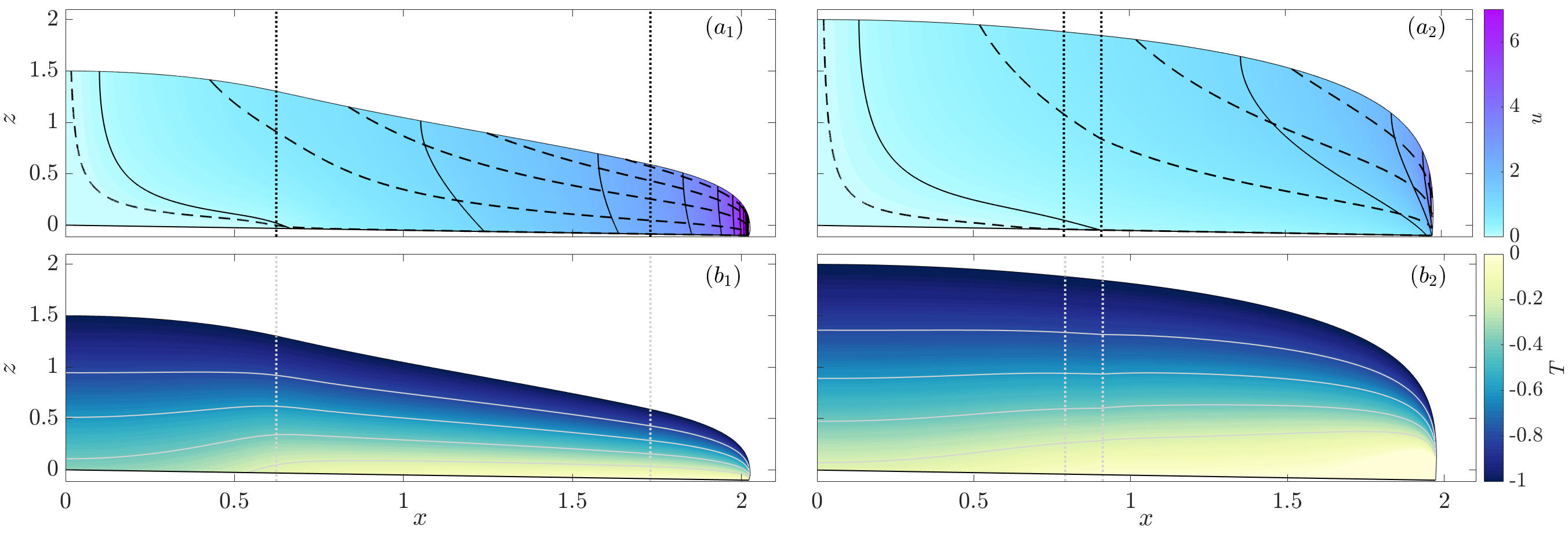
Figure 1: Two-dimensional reference solutions. Panels a₁, b₁ show velocity profiles ($u$ given by solid contours, contour interval 1, background shading) and streamlines (dashed lines) for two different, two-dimensional steady state solutions. Vertical dotted lines demarcate the region in which there is significant sliding at subtemperate basal temperatures. Panels a₂, b₂ show the corresponding temperature profiles (white contours, background shading, contour interval of 0.2). Both examples use $Pe=a=1$, $G=0.5$, $T_{s}=-1$, $\mathrm{d}b/\mathrm{d}x=0.05$, $\delta=0.03$. $\gamma_{0}=0.1$, $h(0)=1.5$ (column a, referred to in the text as reference case 1) and $\gamma_{0}=3$, $h(0)=2$ (column b, reference case 2). Both examples use the temperate friction law (7).

Figure 1 shows two examples of two-dimensional solutions with no lateral structure, obtained by requiring all dependent variables as well as the forcing term $a$ to be independent of $y$. These solutions are a generalization of the results in figure 6 of [11], where solutions are computed for the formal asymptotic limit $\delta\ll 1$ of highly temperature-sensitive sliding. In that case, a sharply defined subtemperate region separates a cold-bedded region upstream from a temperately-bedded region downstream. Within the subtemperate region, bed temperature is (to leading order in $\delta$) equal to the melting point, but sliding occurs at a rate that is slower than for fully temperate bed conditions: sliding velocity is instead controlled by the need to maintain energy balance. This is distinct from the temperate bed, which generally has a net positive energy balance, leading to melting.

Figure 1 shows that, for small but finite $\delta$, we obtain a similar thermal and velocity structure to those computed in [11]. A more systematic demonstration of convergence to the limiting form of [11] as $\delta\rightarrow 0$ is given in the supplementary material §S3. For small but finite $\delta$, we again find an extensive region of significant sliding upstream of the transition to a fully temperate bed, indicated by the dashed vertical lines, with bed temperatures close to but below the melting point.

We use two different parameter combinations in figure 1 as reference cases: column a shows an ice sheet in which sliding is relatively fast (with smaller $\gamma_{0}$), while column b shows an ice sheet in which sliding at the onset of the temperate bed is still slow (with a larger $\gamma_{0}$). The corresponding subtemperate regions are of very different extents, with a longer subtemperate region required to reach temperate conditions for the ice sheet that is able to slide faster. We refer to these two reference cases as ‘1’ and ‘2’, prespectively. In both, we use the simple linear friction law (7).

3.3 Three dimensions: pattern formation

Next, we use the same parameter values but solve for the steady ice sheet in three dimensions, introducing a small amount of stochastic noise to the basal sliding coefficient in the subtemperate region, so that $\gamma=\gamma_{0}(1+\epsilon(x,y))\exp(-T/\delta)$, where $\epsilon(x,t)$ is a small white noise term.

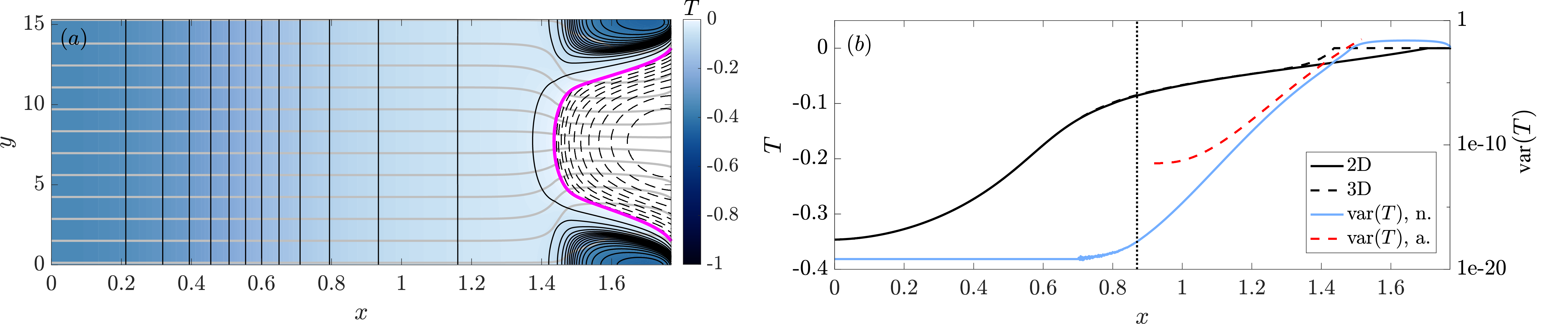
Figure 2: A three-dimensional solution, same parameter choices as figure 1a. Panel a: contours of temperature $T$ (solid lines, also background shading) and $\Pi$ (dashed lines) defined by (51) with $k_{0}=4/3$ and $\Pi_{0}=0.1$, $\beta=1$. Contour levels are 0.025 for $T$, 0.05 for $\Pi$, the subtemperate-temperate boundary is marked in pink. Solid grey lines are streamlines of velocity at the bed. Recall that the length-to-width ratio of the plot is not meaningful: $y$ is measured relative to an ice thickness scale length, $x$ relative to an ice sheet scale length: the evident ice stream pattern is highly elongated in reality. Panel b: Basal temperature against $x$ for the solution in figure 1a (solid black) and in panel a here (dashed black), and the variance in basal temperature with respect $y$ against $x$ (see equation (44); note the logarithmic vertical scale on the right-hand axes). The red dashed curve shows an analytical prediction of the same quantity, see equation (45), with the black dotted vertical line marking the location where $\Lambda$ defined in (42).

An along-flow profile as in figure 1 no longer universally captures the structure that emerges. Figure 2a shows a map of basal temperature against $(x,y)$, obtained for case 1 with stochastic noise applied to $\gamma$. There remains an extended subtemperate region from $x\approx 0.6$ to $x\approx 1.35$, with basal temperatures slowly increasing as we move away from the ice divide. Instead of the transition to a simple temperate bed at $x\approx 1.75$ in figure 1a, a laterally-differentiated pattern rapidly emerges around $x\approx 1.4$ in the three-dimensional calculation, upstream of the subtemperate-temperate transition for the two-dimensional solution. Note that the emergence of this pattern may appear abrupt, but figure 2b reveals that lateral variations in bed temperature actually start to grow a significant distance upstream of the location where see them.

A finger-like region of temperate bed forms in figure 2b, flanked by regions of basal temperatures that decrease with distance downstream, and are much colder than anywhere else under the ice sheet. The streamlines for flow at the ice sheet bed also indicate that the flow of ice rapidly converges into the temperate finger at the onset: this pattern is clearly an ice stream surrounded by ice ridges. Note that here, as in all other calculations in this paper showing formation of a pattern, we find a single temperate ‘finger’ per domain width. That is no accident, as we will show in §4 and discuss further in §5.

The formation of a region of the finger of temperate bed is superficially simple to understand as being the result of a positive feedback between faster sliding at warmer temperatures and greater dissipation of heat at the bed (see §4 below). The pattern formation process is broadly speaking the same as in [10], who however uses the limit of fast sliding throughout the ice sheet. This leads to less sharply defined margins, and also alters the effect of potential negative feedbacks suppressing pattern formation. We discuss these differences further in §5 and the supplementary material §S5.6.

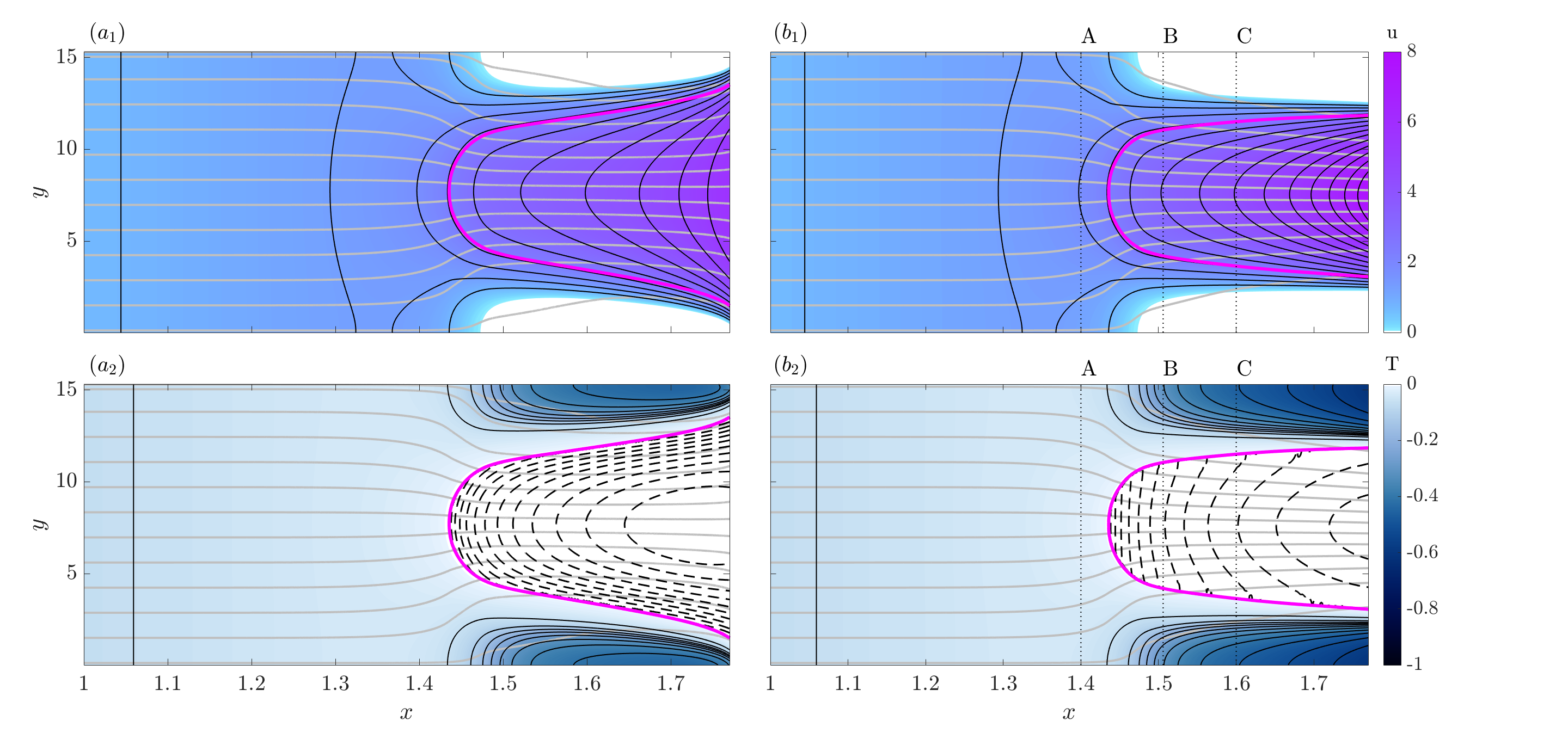
Figure 3: Three-dimensional solutions with different sliding laws: column a) is the same as figure 2, column b) uses the regularized Coulomb friction law with $\mu_{0}=0.005$, $\beta=10$, all other parameter values are identical. Row 2 uses the same plotting scheme as figure 2a with contour intervals of 0.05 for $T$ and $\Pi$, row 1 shows contours of axial velocity $u$ at the bed (as well as background shading), with contour interval 0.5. The pink curve is still the subtemperate-temperate boundary, grey streamlines show velocity at the bed.

Figure 3 shows a close-up of the ice-stream-ice-ridge structure for two cases, the case 1 calculation also shown in figure 2, and a second calculation with the same parameter choices, but the sliding law switched to a regularized Coulomb friction law in the temperate region. Since the solution is obtained by a forward integration in $x$, the plots are identical up to the point where the bed becomes temperate. In addition to basal temperature, each column now also shows basal velocity, confirming that sliding velocities are elevated in the ice stream and continue to increase in the downstream direction.

Importantly, elevated velocities prevail in the region outside of the temperate bed demarcated by the pink lines: in the margins of the ice stream, there is a portion of bed with singificant subtemperate sliding (see also [33]). Sliding is only significantly suppressed where a sharp lateral temperature gradient is evident at the lateral edge of the ice ridge (the edge of the dark blue areas in the second row of figure 3).

The two solutions, for the linear temperate friction law (7) on the left (column a) and for the regularized Coulomb friction law on the right (column b), differ in perhaps unexpected ways. The margins of the ice stream widen more significantly in the downstream direction for the linear friction law, in which the meltwater produced due to dissipation in the ice stream does not feed back into the motion of the ice stream, while for the effective-pressure-sensitive Coulomb law, ice velocity increases much more significantly along the ice stream trunk, but the margins widen only by a small amount. It is likely that the downstream acceleration of the ice stream is responsible, drawing in more ice from the surrounding ice ridges as it lowers the ice surface in the stream, and the attendant lateral heat transport prevents the margins from migrating outwards (see also [32, 33]).

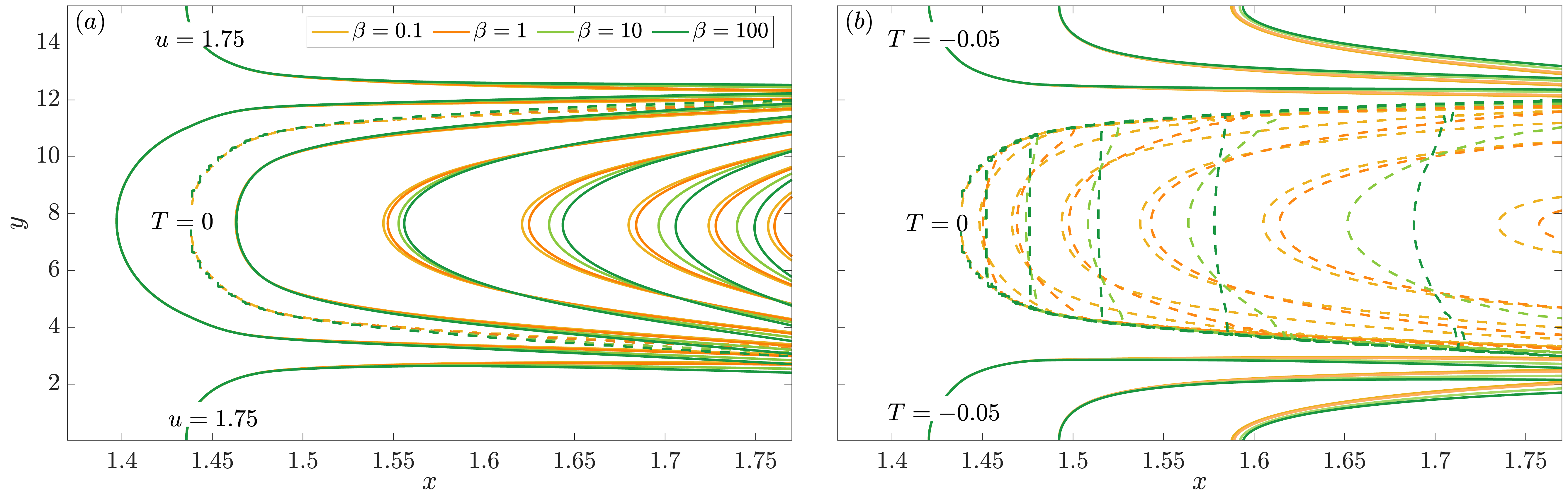
Figure 4: The effect of basal hydrology: solutions of the same problem as column b) in figure 3, but with different values of lateral diffusivities $\beta$ as indicated in the figure legend. Panel a: contours of axial velocity as solid lines, contour inteval 1, dashed line is the subtemperate-temperate boundary. Panel b) contours of temperature as solid lines with contour interval 0,2, $\Pi$ as dashed lines with contour interval 0.1. Contour lines are colour-coded as indicated in the legend in panel a.

In addition to the choice of sliding law, the hydrology model also affects the fully evolved ice stream, although to a much lesser extent. Figure 4 shows solutions for the regularized Coulomb friction law in figure 3b), but with different choices of the diffusion parameter $\beta$ that controls how lateral effective pressure gradients drive the flow of water. As in figures 2 and 3, dashed lines in panel b) show contours of the proxy variable $\Pi\sim N^{-(k_{0}-1)}$ defined in appendix B for a permeability function $\kappa(N)=N^{-k_{0}}$; plotting $\Pi$ rather than $N$ has the advantage that $\Pi$ remains bounded and contours do not become tightly bunched. Key here is to remember that large $\Pi$ corresponds to small $N$ and vice versa. The dashed line in panel a) is the $T=0$ contour.

The effect of $\beta$ on hydrology is obvious in panel b): for a widening ice stream, the proxy $\Pi$ for effective pressure does not typically go to zero near the edge of the temperate region, though $\Pi$ is small there for small diffusivities $\beta$, implying that large effective pressures $N$ are reached. In that case, there are significant lateral gradients in $\Pi$ (or $N$) across the width of the ice stream. For large diffusivities, $\Pi$ (and therefore $N$) becomes nearly constant across the width of the ice stream: lateral drainage is highly effective then, and ensures insignificant variations in basal effective pressure.

As a corollary, we also see that $\Pi$ becomes noticeably larger in the centre of the ice stream for small $\beta$, corresponding to smaller effective pressure $N$, with correspondingly larger sliding velocities (panel a) there for beds with poor lateral drainage, although the velocity difference is quite muted due to the role of lateral shearing in the force balance of the ice stream. By contrast, ice streams with larger $\beta$ and effective lateral drainage widen more rapidly in the downstream direction, although again the effect is muted. This probably occurs because more efficient drainage reduces basal friction towards the edges of the ice stream and thereby concentrates dissipation in the margins themselves, facilitating outward migration [31, 32, 33]

3.4 Cross-sections

We can gain greater insight into the nonlinear pattern forming process by looking at the patterns of axial flow and englacial dissipation as well as of the transverse secondary flow. Figure 5 illustrates these for the ice stream in figure 3b, for which we plot cross-sections across the domain at the locations marked by letters A,B,C in column b) of figure 3.

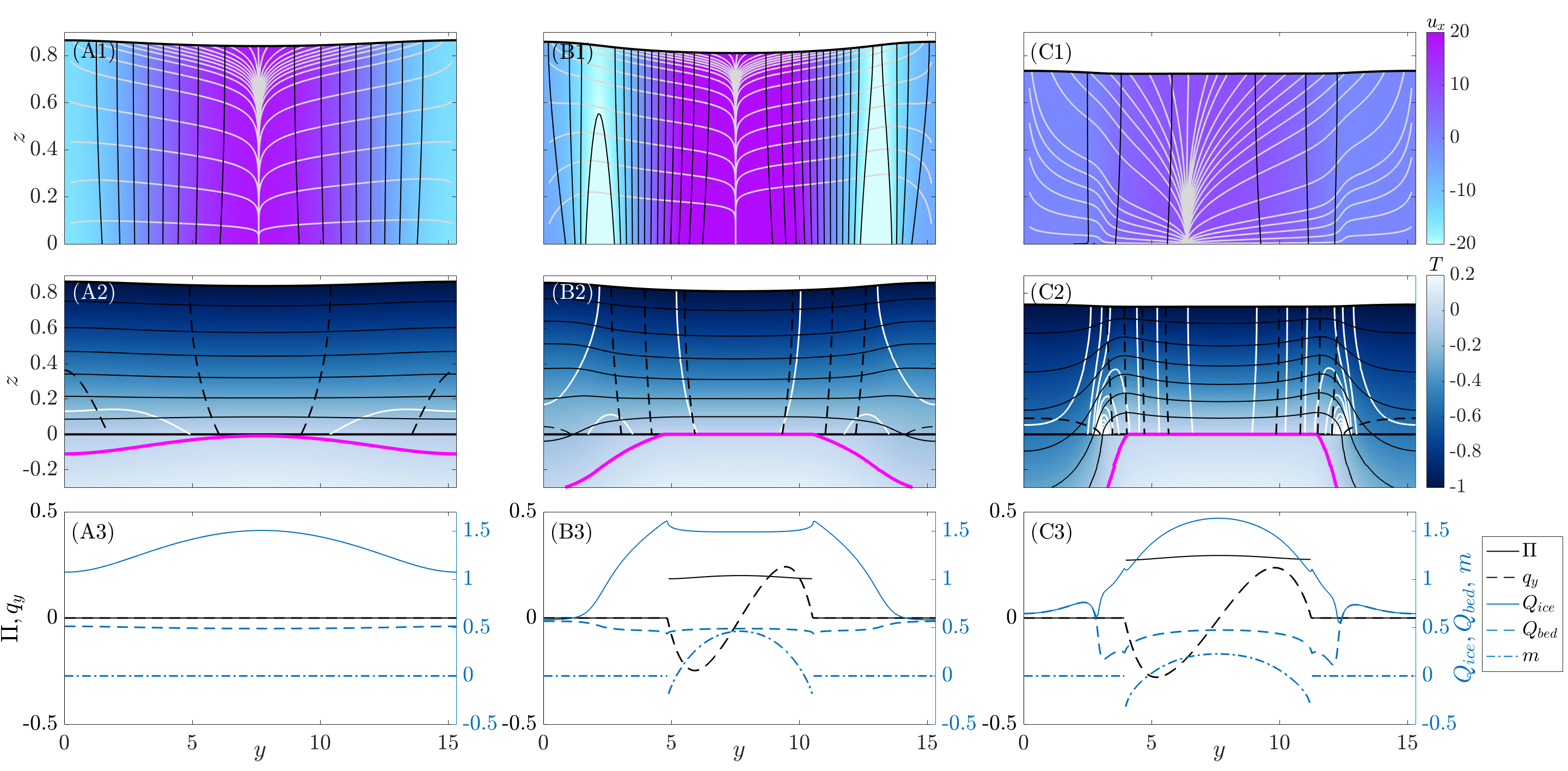
Figure 5: Patterns of flow, dissipation and temperature in the ice, and fluxes at the bed. Each column corresponds to a cross-section indicated by the corresponding letter label in figure 3b. Row 1 (top): contours of ${\partial u}/{\partial x}$ (black, contour interval 4, and background shading), streamlines of $\mbox{\boldmath$v$}_{\perp}$, Row 2 (middle): contours of temperature $T$ (black, contour interval 0.15, and background shading), contours of $u$ (dashed black, contour interval 1) and $\alpha|\nabla_{\perp}u|^{2}$ (white, contour interval 0.5), pink is the $T=0$ contour. Note that part of the bedrock domain is shown. Row 3 (bottom): basal heat flux $Q_{ice}-\lim_{z\rightarrow 0^{+}}{\partial T}/{\partial z}+$ in the ice (solid blue) and $Q_{bed}=-\lim_{z\rightarrow 0^{+}}{\partial T}/{\partial z}$ in the bed (dashed blue), melt rate $m=Q_{bed}-Q_{ice}+\alpha f(T,N,u)|u|$ (dot-dashed blue), effective pressure proxy $\Pi$ (solid black), lateral $q_{y}$ (dashed black).

Each column of figure 5 corresponds to one of these cross-sections, identified by the corresponding letter label. The top row displays isolines of the axial strain rate $u_{x}={\partial u}/{\partial x}$, also indicated by the background colour shading, while the solid white curves are streamlines of the transverse velocity field $\mbox{\boldmath$v$}_{\perp}$. The middle row shows isolines of temperature in black, also indicated by the background colour shading. The pink contour indicates the melting point $T=0$. Dashed contours are velocity isolines, while white contours indicate strain heating rate $\alpha|\nabla_{\perp}u|^{2}$. In all cases, contour intervals are consistent between columns A, B, and C, and in order to illustrate the surface correction $s_{1}$ defined in equation (16), we use $(1+\varepsilon^{2}s_{1}(x,y))z$ as the vertical coordinate for plotting purposes, arbitrarily using a fairly large value $\varepsilon=0.015$ for clarity.

The bottom panel shows aspects of the energy balance of the bed: blue solid and dashed lines are heat fluxes $-{\partial T}/{\partial z}$ at $z=0$, computed in the ice and the bed, repsectively, while the dot-dashed blue line is the net melt rate $m=[{\partial T}/{\partial z}]^{+}_{-}+\alpha f(T,N,u)|u|$. The solid black line is the effective pressure proxy $\Pi$, the dashed black line the later water flux $q_{y}$.

Near the onset of the ice stream (column A), the patterns of englacial flow and dissipation are simple, with a patch of slightly warmer bed in the middle of the domain leading to faster flow (panel A2) and enhanced dissipation (panel A3), where conductive flux $Q_{bed}$ (solid blue line) is elevated at the centre of the domain to balance the additional heat generated at the bed). The faster flow also drawing somewhat colder ice inwards and downwards through a convergent secondary flow (panel A1). Note that there is nothing inconsistent in the streamlines of $\mbox{\boldmath$v$}_{\perp}$ converging (panel A1) despite the flow being incompressible: these streamlines are not actual particle trajectories, as they ignore the simultaneous axial motion of the ice. Note that englacial dissipation also begins to be shifted towards the edges of the region of fast flow.

Somewhat further downstream, the bed has become fully temperate at the centre of the incipient ice stream (panel B2). This coincides with the formation of the very cold-based ice ridges, and the margin of the region of fast flow migrates inwards (even as the margin of the temperate bed migrates outwards, see figure 3b). As a result, the axial strain rate in the incipient ice ridges is locally substantially negative, especially around $y=2.5$ and $y=12.5$ in figure 5B1. The transverse streamlines are therefore locally warped upwards. This contrasts with the usual expectation of ice being drawn downwards as it traverses an ice stream margin [32, 33], but is potentially consistent with specific field observations of englacial radar reflectors near the margins at the upstream end of the Northeast Greenland Ice Stream similarly being warped upwards [43]. It is unclear however whether direct comparisons with field data are a good test of theory, since it is unclear whether the field data in [43] or elsewhere reflect steady state conditions, or indeed whether spatial anomalies in $G$ that are not considered here play a significant role in individual locations (see also [7]).

In column B, significant subtemperate sliding occurs over a region substantially larger than the temperate bed patch at the centre of the domain, as is reflected by the elevated basal heat flux $Q_{bed}$ in panel B3. Inside the temperate bed region, an active drainage system is established. The effective pressure proxy $\Pi$ has a slight gradient, and does not go to zero at the edge of the temperate region. Consequently, the bed retains a finite water content there, and basal shear stress is discontinuous across the subtemperate-temperate boundary. Water flows from the centre of the ice stream, where melt rates $m$ are positive, towards the margins, where there is a small but finite freezing rate (panel B3). This freezing rate is mathematically unavoidable in a margin where basal shear stress is discontinuous and subtemperate sliding occurs (see [33] and §S2 of the supplementary material).

By the time cross-section C is reached, there is a fully-established pattern of an ice ridge in which there is a simple transverse ‘shallow-ice’ type shearing flow towards the margin, a clearly defined margin, and a lateral-shear-dominated ice stream as described by [32]. In fact, for a wide domain, it can be shown that the model we use here is equivalent to the parameter regime described in appendix B of [44]; the advantage of our model over that in [32] is that we are able to capture the onset of the ice stream in addition to the fully evolved form.

The axial strain rate ${\partial u}/{\partial x}$ is now significantly smaller than in the region of rapid flow reorganization around cross-sections A and B, and shows a noticeable asymmetry (panel C1): the ice stream does not initiate perfectly symmetrically, and as a result its margins do not migrate outwards symmetrically, giving the now much weaker secondary flow a corresponding asymmetry, with convergence not centered on the middle of the stream. As a result of the weaker secondary flow, the surface correction $s_{1}$ is now also less pronounced than in the onset region, and has the familiar pattern of a convex surface over the ice ridges, and a flat surface over the ice stream.

The margins exhibit the strongly concentrated englacial dissipation (panel C2) familiar from previous studies [45, 46, 47, 31, 48, 32, 49, 33, 50], and advection due to the secondary flow is angled sharply downward through the margins (panel C1). The competition between these two and the effect of basal dissipation due to subtemperate sliding ultimately control margin migration [33], although here in the sense of ice stream widening in the downstream direction, rather than in time.

Two observations may be significant: first, the strong concentration of shear does not occur at the transition from a temperate to a subtemperate bed. Instead, it coincides with a sharp lateral temperature gradient between small negative temperatures near the edge of the ice stream, accompanied by fast subtemperate sliding, and the much lower basal temperatures of the ice ridge. Secondly, no temperate ice is formed at this location, with englacial temperatures remaining firmly below the melting point. Both observations are consistent with previous work on subtemperate sliding in shear margins [33], though it is conceivable that the absence of temperate ice is the result of the moderate width of the modelled ice stream [51, 50, 52]

The temperate bed portion of the ice stream exhibits a similar though slightly more complicated pattern to cross-section B. Basal dissipation is concentrated at the centre of the ice stream, where net melt occurs, and a relatively weak later gradient in $\Pi$ suffices to drive water towards the margins, where there is a small but finite rate of melting, and $\Pi$ remains finite. at the cold-temperate transition.

3.5 Other forms of patterning, or no pattern at all

All ‘patterned’ three-dimensional solutions that we have described so far are based on the two-dimensional reference case 1 of figure 1a. Even if we apply a stochastic perturbation to $\gamma$ in reference case 2 of figure 1b, no pattern emerges in three dimensions in the much shorter subtemperate area, in which sliding velocities are also much slower. If we continue the calculation as in figure 1b with a linear friction law (7), no pattern emerges at all even downstream of the cold-temperate transition, and we simply recover the solution in figure 1b with a small amount of noise.

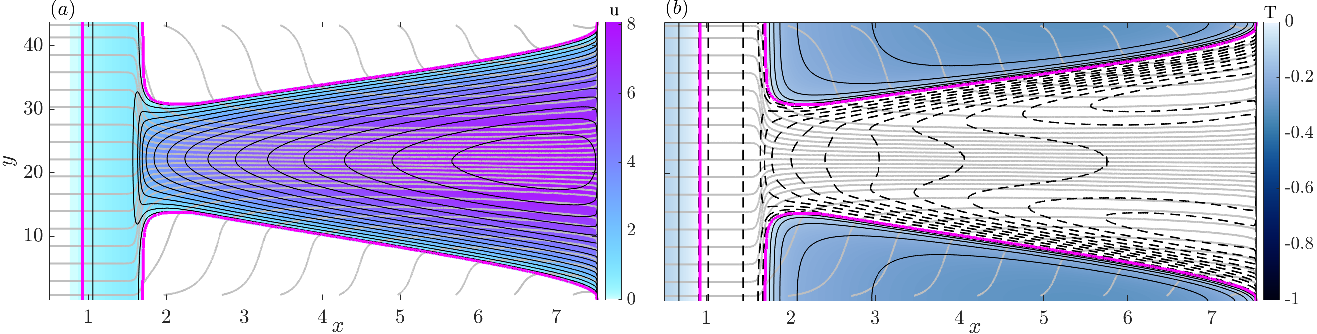
Figure 6: Hydromechanical instability: same parameters as figure 1b but using the double power law (8) and $N$ and $\tilde{\kappa}$ defined through (51) with $\Pi_{0}=0.1$, $N_{s}=0.1$, $k_{0}=4/3$, $\beta=0.1$. Same plotting scheme as figure 3, contour interval of 1 for $u$, 0.15 for $T$, 0.1 for $\Pi$

A pattern can still emerge from within the temperate area if we use an effective-pressure-dependent sliding law: figure 6 is analogous to figure 3 but for reference case 2 with a power-law friction (8). The entire bed becomes temperate around $x\approx 0.9$, with no apparent patterning as described above. Around $x\approx 1.7$ a pattern then rapidly emerges, with a patch of low effective pressure $N$ (large $\Pi$) facilitating enhanced sliding and drawing in ice through the secondary transverse flow. The ice flow surrounding the patch of low effective pressure slows (as it must, with total ice flux being prescribed), dissipation there is reduced and the bed actually refreezes.

Once again, an ice-stream-ice-ridge pattern forms, with very low bed temperatures in the ice ridges. One notable feature of the solution is the formation of a double-peaked, off-centre maximum in the effective pressure proxy $\Pi$ in the fully evolved ice stream, corresponding to a double minimum in $N$. This is partly the result of the low diffusivity $\beta$ not smoothing basal effective pressure, but primarily results from englacial dissipation: strong shearing near the margins of the ice stream (which is substantially wider than in figure 3) warms the ice (though never to the melting point). Advection carries this warmer ice towards the centre of the ice stream, and the reduced conductive heat flux at the bed causes additional melting at an intermediate position between margin and ice stream centre, leading to the observed effective pressure distribution. As in the case of the pattern emerging from subtemperate sliding, we can look at cross-sectional patterns of flow, dissipation and temperature in the ice to understand this pattern better, see supplementary material §S3.

The formation of the ice-steam-ice-ridge pattern in this case is closely related to the mechanisms in [5, 6, 7], as discussed further in §5. Patterning in this instance is driven by a hydromechanical positive feedback between dissipation, increased discharge of additional meltwater requiring reduced effective pressure, and reduced effective pressure leading to faster sliding and increased dissipation. This feedback does not, however, unconditionally lead to the formation of a recognizable ice stream pattern: in the supplementary material §S3, we showcase an example in which a slight lateral perturbation in effective pressure and velocity grows over a limited stretch of the ice sheet, only to disappear again further downstream, without ever forming a distinct ice stream margin.

In fact, for many plausible parameter choices, we have found no pattern formation due to the the hydromechanical feedback at all. Overall, the question of negative feedbacks that act to suppress pattern formation remains open. We address this next.

4 Stability analysis

The numerical solutions in the previous section raise the question of why (and where) patterning appears in some of the steady state solutions, but not others. Here, we show that patterning can be understood as a ‘spatial’ instability. Rather than asking whether perturbations to a laterally uniform steady state grow in time, we use the time-like nature of $x$ to identify conditions under which perturbations in upstream conditions (at the divide) or in forcing (such as the stochastic perturbations to $\gamma_{0}$ that we have used numerically) are amplified as we move downstream. Similar notions of spatial stability have previously been used to study the growth of basal channel along the base of an ice shelf [53] as well as ice stream formation using a simpler model than ours [5].

We conduct our linear stability analysis in the limit of small $\delta$, and confine ourselves to the case of patterning in the subtemperate region. We will show that patterns can grow in the downstream direction if sliding velocities in the subtemperate region exceed a certain threshold. The hydraulically-controlled onset of patterning during temperate sliding is studied in more detail in the supplementary material (§S5.7), as is the onset of patterning during subtemperate flow for the more general case $\delta=O(1)$ (§§S5.1–S5.4).

Recall that $\delta\ll 1$ is the bed temperature scale over which the ice sheet transitions from insignificant to fully temperate sliding. We can identify a similarly short thermal boundary layer length scale $z\sim\delta$ over which those temperature variations occur naturally near the bed, and a corresponding along-flow distance scale $x\sim\delta^{2}$ such that advection and diffusion balance in the basal thermal boundary layer for $Pe\sim O(1)$ (see also [19]). This turns out to be (formally) the length scale over which the onset of patterning takes place in figure 2. We can capture the dominant processes involved by rescaling

$$Z=\delta^{-1}z,\qquad X=\delta^{-2}x,$$ (31)

and putting $\Theta(X,y,Z)=\delta^{-1}T(x,z)$. $X$ is a local along-flow coordinate, while $Z$ is distance above the bed in the thermal boundary layer; $z$ will continue to describe distance above the bed in the ‘outer’ region that occupies most of the ice thickness. Implicit here is that $\delta^{2}\gg\varepsilon$ where $\varepsilon$ is the ice sheet aspect ratio, so that the local variable $X$ still describes displacements that are much larger than the ice thickness scale, and the shallow-in-$x$ model of §2 continues to apply.

A rapid onset also alters the scale for the secondary ice flow, as faster transverse velocities are required to balance the potentially large velocity gradient ${\partial u}/{\partial x}\sim O(\delta^{-2})$. We put $U_{o}(X,y,z)=u(x,y,z)$, $V_{o}(X,y,z)=\delta^{2}v(x,y,z)$, $W_{o}(X,y,z)=\delta^{2}w(x,y,z)$, $P_{o}=\delta^{2}p(x,y,z)$ in the outer region, distant from the bed, and put $U_{b}(X,y,Z)=U_{o}(X,y,z)$, $V_{b}(X,y,Z)=V_{o}(X,y,z)$, $W_{b}(X,y,Z)=\delta^{-1}W_{o}(X,y,z)$ in the thermal boundary layer, the latter to account for the fact that vertical velocity vanishes at the bed. A rescaling of the mechanical problem to the thermal boundary layer variable $Z$ and matching with its outer version shows that $U_{b}=U_{o}(x,y,0)$, $V_{b}=V_{o}(x,y,0)$ and $W_{b}=W_{bZ}Z$, where $W_{bZ}={\partial W_{b}}/{\partial Z}=\lim_{z\rightarrow 0}{\partial W_{o}}/{\partial z}$, and $U_{b}$, $V_{b}$, $W_{bZ}$ are all independent of $Z$ at leading order.

Ice thickness remains constant at leading order over the scale associated with the variable $X$, which really describes an internal layer with respect to the outer coordinate $x$ inside the ice sheet, but the surface slope may change by $O(1)$. Formally, this can be accounted for by putting $H(X)=h(x)$ and expanding $H(X)=\bar{H}+\delta^{2}H_{1}(X)$, so that $\mathrm{d}h/\mathrm{d}x=\mathrm{d}H_{1}/\mathrm{d}X$ while ice thickness remains constant at $\bar{H}$. In full, the mechanical problem consisting of (4), (5), (13), (14)–(15) and (17)–(18) becomes

$$\nabla_{\perp}^{2}U_{o}=-\frac{\partial b}{\partial x}-\frac{\partial H_{1}}{\partial X}\quad\mbox{on }0<z<\bar{H},\quad\frac{\partial U_{o}}{\partial z}=\Gamma(\Theta(0))U_{o}\quad\mbox{on }z=0,\qquad\frac{\partial U_{o}}{\partial z}=0\quad\mbox{on }z=\bar{H},$$ (32a)

where $${\partial b}/{\partial x} X \Gamma(\Theta)=\gamma(T) \mathrm{d}\Gamma/\mathrm{d}\Theta\sim O(1)$$ is constant at the inner horizontal scale associated with and , and the rescaling ensures that . In addition

$$\nabla_{\perp}^{2}(V_{o},W_{o})-\nabla_{\perp}P_{o}=0,\quad\frac{\partial V_{o}}{\partial y}+\frac{\partial W_{o}}{\partial z}=-\frac{\partial U_{o}}{\partial X}$$ (32b)

on $$0<z<\bar{H}$$, subject to

$$W_{o}=0,\quad\frac{\partial V_{o}}{\partial z}+\frac{\partial W_{o}}{\partial y}=\Gamma(\Theta(0))V_{o}/U_{o}\quad\mbox{at }z=0,\quad W_{o}=\frac{\partial V_{o}}{\partial z}=0\quad\mbox{at }z=\bar{H}$$ (32c)

while the surface perturbation $$H_{1}(X) (y,z) Q=\int_{0}^{W}\int_{0}^{\bar{H}}U\mathrm{d}z\mathrm{d}y=$$ is independent of and determined by the constraint constant.

At leading order, we obtain a thermal boundary layer problem of the form

$$Pe\left(U_{b}\frac{\partial\Theta}{\partial X}+V_{b}\frac{\partial\Theta}{\partial Y}+W_{bZ}Z\frac{\partial\Theta}{\partial Z}\right)-\frac{\partial^{2}\Theta}{\partial Z^{2}}= 0 \mbox{for }Z>0$$ (33a)

$$-\frac{\partial^{2}\Theta}{\partial Z^{2}}= 0 \mbox{for }Z<0$$ (33b)

$$\left[-\frac{\partial\Theta}{\partial Z}\right]_{-}^{+}= \Gamma(\Theta(0))U_{b}^{2},\qquad[\Theta]_{-}^{+}=0 \mbox{at }Z=0,$$ (33c)

The outer thermal problem is advection-dominated in the ice and diffusion-dominated in the bed. At leading order, matching of (33) with the far field therefore requires that

$$U_{b}\frac{\partial\Theta}{\partial X}+V_{b}\frac{\partial\Theta}{\partial Y}+W_{bZ}Z\frac{\partial\Theta}{\partial Z}\sim 0\qquad\mbox{and}\qquad-\frac{\partial\Theta}{\partial Z}\sim-\lim_{z\rightarrow 0^{-}}\frac{\partial\Theta}{\partial z}=G$$ (34)

as $Z\rightarrow+\infty$ and $Z\rightarrow-\infty$, respectively.

The solutions without lateral structure computed in §33.2 are functions of $x$ and $z$, and consequently are constant in the rescaled variable $X$ at leading order. If we take those two-dimensional solutions as a base state and consider their stability to pattern formation in three dimensions with $X$ as the time-like variable, we can therefore linearize and treat the base state as uniform. Denoting the base state by overbars and putting $\theta=-(h+b)_{x}$, evaluated locally, we have $\bar{V}_{b}=\bar{W}_{bz}=0$ and $\bar{\Gamma}\bar{U}_{b}=h\theta$, where $\bar{\Gamma}=\Gamma(\bar{\Theta}(0))$, as well as $\bar{\Theta}=\bar{\Theta}(0)-GZ$ for $Z<0$ and $\bar{\Theta}=\bar{\Theta}(0)-(G+\bar{\Gamma}\bar{U}_{b}^{2})Z$ for $Z>0$. We perturb the base state as

$$U_{b}=\bar{U}_{b}+U_{b}^{\prime}\exp(\Lambda X+iky),\qquad V_{b}=V_{b}^{\prime}\exp(\Lambda X+iky),\qquad W_{z0}=\bar{W}_{z0}+W_{z0}^{\prime}Z\exp(\Lambda X+iky),$$

$$\Theta=\bar{\Theta}(Z)+\Theta^{\prime}(Z)\exp(\Lambda X+iky),$$ (35)

and linearize in the perturbations, where we assume that $k\neq 0$; since the ice thicness variation term $H_{1}$ is independent of $y$, there is then no need at first order to incorporate $H_{1}$ in the linearization.

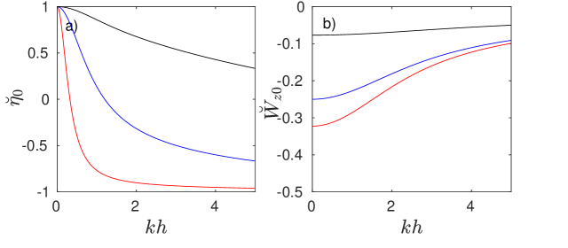
Figure 7: Plots of $\breve{\eta}_{0}=\eta_{0}/(-\alpha\bar{\Gamma}_{\Theta}\bar{U}_{b}^{2})$ (panel a) and $\breve{W}_{z0}=W_{z0}/(-\bar{\Gamma}_{\theta}\bar{U}_{b}h)$ (panel b) as functions of $kh$ for $\bar{\Gamma}h$ = 0.1 (red), $\bar{\Gamma}h$ = 1 (blue) and $\bar{\Gamma}h=10$ (black). Note that $\breve{\eta}_{0}$ and $\breve{W}_{z0}$ thus defined are functions of $\bar{\Gamma}h$ and $kh$ only. As $\bar{\Gamma}_{\Theta}<0$, $\breve{\eta}_{0}$ and $\breve{W}_{z0}$ also have the same sign as $\eta_{0}$ and $W_{z0}$, respectively. Physically $\eta_{0}$ represents the feedback between bed temperature and basal dissipation for a given wavenumber, while $W_{z0}$ represents the effect of basal temperature on vertical advection near the bed.

In the usual fashion, a positive growth rate $\Re(\Lambda)$ indicates the growth of perturbations, albeit in the downstream direction rather than in time. Solving the appropriate linearized version of (32), we find that the perturbations in vertical velocity gradient and in basal dissipation can be expressed in terms of $\Theta^{\prime}(0)$ as

$$W_{bZ}=W_{z0}\Theta^{\prime}(0),\qquad 2\bar{\Gamma}\bar{U}_{b}U_{b}^{\prime}+\Gamma^{\prime}\bar{U}_{b}^{2}=\eta_{0}\Theta^{\prime}(0),$$ (36)

where $\Gamma^{\prime}=\Gamma_{\Theta}\Theta^{\prime}(0)$ is the perturbation in $\Gamma$, and

$$W_{z0}= \bar{\Gamma}_{\Theta}\bar{U}_{b}h\frac{\sinh(kh)\cosh(kh)-kh}{2kh\sinh^{2}(kh)+\bar{\Gamma}h[\sinh(kh)\cosh(kh)-kh]},$$ (37)

$$\eta_{0}= -\alpha\bar{\Gamma}_{\Theta}\bar{U}_{b}^{2}\frac{\bar{\Gamma}h\cosh(kh)-kh\sinh(kh)}{\bar{\Gamma}h\cosh(kh)+kh\sinh(kh)}.$$ (38)

Here and below, we use the shorthand $\bar{\Gamma}_{\Theta}=\mathrm{d}\Gamma/\mathrm{d}\Theta|_{\Theta=\bar{\Theta}(0)}$. The functions $W_{z0}$ and $\eta_{0}$ are plotted in figure 7.

Since basal friction decreases with increasing temperature, we have $\bar{\Gamma}_{\Theta}<0$. Defining the unperturbed basal heat flux above the bed as $Q_{0}=-\lim_{Z\rightarrow 0^{+}}\mathrm{d}{\bar{\Theta}}/\mathrm{d}{Z}=G+\bar{\Gamma}\bar{U}_{b}^{2}$, equal to the sum of geothermal heat flux and the unperturbed basal dissipation rate, the linearized heat equation in the basal boundary layer (33a) becomes

$$\Lambda\left(Pe\,\bar{U}_{b}\Theta^{\prime}(Z)-Pe\,W_{z0}Q_{0}Z\Theta^{\prime}(0)\right)-\frac{\textrm{d}{{}^{2}\Theta^{\prime}}}{\textrm{d}{Z^{2}}}=0$$ (39a)

for $$Z>0 \mathrm{d}\Theta^{\prime}/\mathrm{d}Z=0 Z<0$$, while the heat equation (33b) in the bed trivially yields for . The boundary and matching conditions (33c)–(34) become

$$\frac{\textrm{d}{\Theta^{\prime}}}{\textrm{d}{Z}}+\eta_{0}\Theta^{\prime}=0\qquad\mbox{at }Z=0,\qquad\frac{\textrm{d}{\Theta^{\prime}}}{\textrm{d}{Z}}\sim W_{z0}Q_{0}/\bar{U}_{b}\qquad\mbox{as }Z\rightarrow\infty.$$ (39b)

The eigenvalue problem (39) can also be derived as a parametric limit for $\delta\ll 1$ from a more general spatial stability problem for a parallel-sided slab of ice subject to subtemperate sliding at its base, as described in the supplementary material §S5.5. (39) has solution

$$\Theta(Z)=\Theta(0)\left[\exp\left(-\sqrt{\Lambda Pe\,\bar{U}_{b}}Z\right)+\frac{W_{z0}Q_{0}Z}{\bar{U}_{b}}\right],$$ (40)

where the eigenvalue $\Lambda$ satisfies $\sqrt{\Lambda Pe\,\bar{U}_{b}}=\eta_{0}+W_{z0}Q_{0}/\bar{U}_{b}$, and $\sqrt{\Lambda Pe\,\bar{U}_{b}}$ must have positive real part (and therefore must be real and positive) in order to satisfy the matching condition (39b)₂. Hence we require

$$\eta_{0}+\frac{Q_{0}W_{z0}}{\bar{U}_{b}}>0,$$ (41)

for a solution of this form to exist.

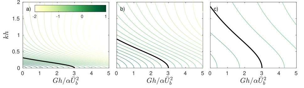
Figure 8: Contours of $\breve{\eta}_{0}+(\bar{\gamma}h+Gh/(\alpha\bar{U}_{b})^{2})\breve{W}_{z0}=(\alpha\bar{\Gamma}_{\Theta}\bar{U}_{b}^{2})^{-1}(\eta_{0}+Q_{0}W_{z0}/\bar{U}_{b})$ against $kh$ and $Gh/(\alpha\bar{U}_{b}^{2})$ for $\bar{\gamma}h=0.1$ (panel a), $\bar{\gamma}h=1$ (panel b) and $\bar{\gamma}h=10$ (panel a). See figure 7 for the definitions of $\breve{\eta}_{0}$ and $\breve{Q}_{z0}$. The solid black is the zero contour. A viable solution of the form (40) exists if the contoured quantity is positive (below the solid black line), in which case the growth rate is proportional to the square of the contoured quantity, see equation (42), and the solution is automatically unstable.

When (41) is satisfied, the eigenvalue is positive and instability results:

$$\Lambda=\frac{1}{Pe\,\bar{U}_{b}}\left(\eta_{0}+\frac{W_{z0}Q_{0}}{\bar{U}_{b}}\right)^{2}.$$ (42)

Note that $\eta_{0}$ is positive for small $k$ but changes sign at some finite $k$, while $W_{z0}$ is always negative (figure 7). Consequently, we have stabilization of small wavelengths, since (41) is violated for large enough $k$. Recall that $\eta_{0}$ represents the feedback between raised basal temperature $\Theta^{\prime}(0)$ and dissipation at the bed (see equation (36)). That feedback consists of two competing components: raising $\Theta^{\prime}(0)$ has the direct effect of reducing the basal friction coefficient, and therefore of reducing basal dissipation (the second term on the left-hand side of (36)₂). It also has the indirect effect of allowing faster sliding, which increases dissipation (the first term on the right-hand side). At short transverse wavelengths, or large $k$, basal velocity variations are suppressed by lateral shear stress is in the ice [54, 55], and the negative feedback dominates. At larger transverse wavelengths, these basal velocity variations invariably become large enough to dominate the feedback mechanism.

The stability criterion (41) shows that we must have a positive feedback with $\eta_{0}>0$ in order for instability to occur as described, but that is insufficient; $\eta_{0}$ must in fact exceed a positive threshold $-W_{z0}Q_{0}/\bar{U}_{b}$, which represents the stabilizing effect of downward advection of cold ice as the downstream velocity $\bar{U}_{b}$ increases.

Next, we extract from (41) an explicit criterion for instability in terms of model parameters. The dispersion relation (42) demonstrates that there is no wavelength selection at long wavelengths: if there is an unstable mode for a given set of parameters, the fastest growing wavenumber is always the limit $k\rightarrow 0$ (or $kh\rightarrow 0$, see figure 8). This is consistent with only a single ice stream forming in the domain in the numerical solutions (see also §5 and supplementary material §S5.9–S5.10. In the limit $k\rightarrow 0$, we have $\eta_{0}\sim-\alpha\bar{\Gamma}_{\Theta}\bar{U}_{b}^{2}$, $W_{z0}\sim\bar{\Gamma}_{\Theta}\bar{U}_{b}h/(\bar{\Gamma}h+3)$, as well as $Q_{0}=\alpha\bar{\Gamma}\bar{U}_{b}^{2}+G$, so that (42) gives $\sqrt{Pe\,\bar{U}_{b}\Lambda}\sim-\alpha\bar{\Gamma}_{\Theta}\bar{U}_{b}^{2}\left[3/(\Gamma h)-G/(\alpha\bar{\Gamma}\bar{U}_{b}^{2})\right]/\left[1+3/(\bar{\Gamma}h)\right]$ and we see that the criterion for instability (the right-hand side of the equation is positive) is that $Gh/(\alpha\bar{U}_{b}^{2})<3$, or

$$\bar{U}_{b}^{2}>\frac{Gh}{3\alpha}.$$ (43)

This is the criterion we seek: for a given geothermal flux $G$, Brinkmann number $\alpha$ and ice thickness $h$, the subtemperate sliding velocity $\bar{U}_{b}$ needs to exceed a threshold value before the spatial pattering instability first occurs in the manner predicted above.

Note that the instability criterion is based on the ‘viability’ of the thermal boundary layer solution, through requiring that the eigenfunction solution (40) can match with an advection-dominated outer region, with the exponential part of the solution decaying in $Z$. If there is no viable solution of the form (40), this does not mean that we cannot formulate a stability problem, or even that there is necessarily no instability. It does mean that any growing mode is no longer of a boundary-layer type, and does not grow at rapidly with $\Lambda\sim\delta^{-2}$: instead, we obtain slowly growing solutions that satisfy $T^{\prime}=0$ at $z=0$ at leading order. These can in fact have eigenvalues with real parts. However, the corresponding e-folding lengths are then comparable with ice sheet length, contrasting with e-folding lengths of $\delta^{2}$ times ice sheet length for the boundary layer solution (40): in that case, an initial perturbation might grow by a multiple of itself over the full length of the subtemperate region, but is unlikely to lead to a fully formed ice stream. The supplementary material provides further detail in §S4.

The instability criterion (41) explains why there is an extended region of slower subtemperate sliding upstream of the rapid transition to patterned flow in figure 2: patterning does not occur as soon as appreciable sliding appears. Recall however that figure 2a is misleading, since the point at which we perceive the pattern is a fairly large number of spatial $e$-folding lengths from the location at which pattern growth is initiated, depending on the level of noise in the system. This is illustrated in figure 2b, which shows the lateral variance of basal temperature,

$$\mathrm{var}(T)(x)=W^{-1}\int_{0}^{W}\left[T(x,y,0)-W^{-1}\int T(x,y^{\prime},0)\mathrm{d}y^{\prime}\right]^{2}\mathrm{d}y,$$ (44)

as a function of $x$. We see that $\mathrm{var}(T)$ begins to grow at $x\approx 0.7$, while the pattern does not reach an $O(1)$ amplitude, with the bed becoming partly temperate, until $x\approx 1.4$.

In fact, the dispersion relation (42) predicts that pattern growth should start at a location further downstream ($x\approx 0.9$) than the location where $\mathrm{var}(T)$ actually starts to exhibit approximately exponential growth at comparable rates to those predicted by (42). The red curve in 2a₃ shows a plot of

$$\mathrm{var}_{\infty}(T)(x)=c\exp\left(2\delta^{-2}\int_{x_{0}}^{x}\Lambda(x^{\prime})\mathrm{d}x^{\prime}\right)$$ (45)

against $x$, the constant $c$ chosen to make the plot visible and $x_{0}$ being the first location at which a viable solution (42) to the eigenvalue problem appears, having linearized locally around the two-dimensional reference solution in figure 1a and chosen $k=2\pi/W$ as the smallest non-zero to fit into the domain. The formula (45) is the form of the variance in $T$ one would expect from our linearized problem if we account for the fact that parameters in the linearization change slowly with $x$.

Clearly, the red curve in 2b misses part of the original growth in the variance shown in blue. The most likely explanation for why equation (42) underpredicts pattern growth is that the asymptotic solution relies on separation into an inner region in which diffusion appears at leading order, and an outer region in which the temperature problem is advection-dominated: (39b) arises from a purely advective temperature field in the outer region, justified at leading order because $\delta^{-2}Pe\gg 1$ is the effective Péclet number in the outer region. In advection-diffusion problems, the effects of diffusion can be significant even at relatively large Péclet numbers (see, e.g., [33] for a glaciological example). We demonstrate in the supplementary material (§S5.5) that this is also the case here, by comparing the asymptotic solution presented above with a stability analysis that resolves the full depth of the ice. .

Nonetheless, the effectively conditional nature of the spatial instability explains why, in some cases, there is no pattern formation at all in the subtemperate region: subtemperate sliding speeds may never get large enough to exceed the threshold value for initiating pattering, as is the case for reference case 2 in figure 1b. In fact, even if that threshold is passed, unstable growth of the pattern may not need to lead to a fully formed ice stream if the region of subtemperate sliding is too short and therefore comprises too few e-folding length scales before the boundary with the temperate bed is reached.

5 Discussion

We have modelled the formation of ice streams through positive feedbacks between sliding and dissipation at the bed, using a novel thermomechanical model that combines ‘shallow ice’ balances in the along-flow direction with the ability to resolve fully lateral shear stress and the secondary transverse flow required by mass conservation. The model is the natural generalization of early work on thermomechanical ice sheet flow by Hutter et al. [13] and Yakowitz et al. [14]. Our focus has been on sliding that occurs at temperatures below the melting point, when basal friction is temperature-dependent.

In that case, the feedback is simple: locally warmer temperatures reduce friction, and will lead to faster sliding. How much faster depends on the length scales involved: for warmer temperatures confined to a narrow region (or a periodic temperature perturbation with a short wavelength, comparable to ice thickness or smaller for a subtemperate flow with significant vertical shearing), the acceleration in flow will be suppressed by lateral shear stresses. Local warming of the bed results in a net increase in basal dissipation and therefore further heating if basal temperatures are elevated over a sufficiently large span of the bed (i.e., if the basal temperature perturbation has a sufficiently long lateral wavelengths): the reduction in friction in isolation has the effect of reducing dissipation. Faster sliding, not affected excessively by lateral shear stresses, is key to increased dissipation.

In a steady state setting, the positive feedback can lead to ice flow accelerating with distance in the downstream direction to form a ‘finger’ of faster-flowing ice surrounded by slower-moving ice: an incipient ice stream. In doing so, the accelerating flow will draw in colder ice from above and the sides, generating a negative cooling feedback that must be overcome. That is the basis of the pattern-forming instability criterion (41). Where this is satisfied, our model predicts a length for the size of the onset region as $\delta^{2}$ times ice sheet length, where in dimensional terms $\delta^{-1}=\gamma_{T}(T_{s}-T_{m})/\gamma$, $\gamma_{T}$ being the (dimensional) temperature derivative of the basal friction coefficent $\gamma$ at the melting point $T_{m}$, and $T_{s}$ being surface temperature. When pattering occurs over a sufficiently short distance downstream, a fully evolved ice stream-ice ridge pattern forms downstream, with sharply defined margins that slowly move apart in the downstream direction (§§33.3–3.4).

Being able to resolve the margins helps reveal the significant (typically $\sim$ one ice thickness wide) region of subtemperate bed that lies inside the ice stream as defined by the velocity pattern (figures 3 and 5). Such a zone of rapid subtemperate sliding at the edge of an ice stream was previously predicted by [33]. Resolving the margins and the processes that cause their position to shift allows us to explore the effect of different parameterizations of basal friction and hydraulics on ice stream geometry: for instance, we find that drainage systems with more efficient lateral transport tend to generate ice streams that widen more significantly in the downstream direction, but have higher effective pressures and lower velocities in the ice stream center (figure 4).

The clearest precursor to our work is due to Hindmarsh [10]. While he motivates his model by appealing to concentrated, temperature-dependent shear near the bed, Hindmarsh’s mathematical formulation is a plug flow, implying fast sliding, with friction a relatively slowly varying function of temperature. These two constraints correspond to the limit of $\delta\sim O(1)$ and $\gamma_{0}\ll 1$ in our model.

While our model can be solved and analyzed for Hindmarsh’s parameter regime, our analysis has focused on the alternative regime of a shearing flow in which friction is highly sensitive to basal sliding ($\delta\ll 1$, $\gamma_{0}\sim O(1)$). The latter choice of parameter regime conforms to the expectation that basal sliding is significant only at temperatures close to the melting point [56, 57, 11, 19]. There are some graphically obvious differences between the solutions, with our model allowing the formation of narrow margins and incorporating a hydrological component (which the model description in [10] does not mention), the two limits used here and in Hindmarsh’s prior work have less obvious but still important differences.

The most significant is the role of downward advection of cold ice in potentially preventing steady state patterns from forming in our analysis in §4. That downward advection is closely associated with a vertical ice column being able to accommodate at least some shearing. For a pure plug flow, an acceleration in the downstream direction is still balanced purely by a commensurate acceleration in the secondary, transverse flow, which is however then also a plug flow and has no significant vertical component (see supplementary material §S5.6). As a result, the case of rapid subtemperate sliding is potentially more prone to pattern formation.

Where no pattern emerges in the region of subtemperate sliding, the hydrological component of our model also captures the alternative, hydromechanical feedback mechanism for ice stream formation due to [5] and [6, 7] within a unified framework. Here, bed temperature is fixed at the melting point. Instead, a region of depressed effective pressure will, for a typical basal friction law, lead to reduced friction, faster flow and, for a sufficiently wide such region, to greater basal dissipation in much the same way as the temperature-dissipation feedback. With a hydraulic model in which the additional melt that results must be evacuated through an enlarged set of basal conduits at a reduced effective pressure, a positive feedback results. This can likewise lead to the formation of an ice-stream-ice-ridge pattern.

One of the advantages of our work over previous models of hydromechanical pattern formation [5, 6, 7] is in fact our ability to capture the refreezing of the bed that occurs in the ice ridges, and the thermomechanics of the margins: one notable difference between our results and those in [6, 7] is that our ice stream widens in the downstream direction, while theirs narrows, which may be the result of our model incorporating englacial heating and a more careful treatment of heat transport: the thermal model in Fowler and Johnson [5] and Kyrke-Smith et al. [6, 7] is based on a similarity solution for a two-dimensional thermal boundary layer due to [58], without lateral heat transport. The validity of that thermal model, especially in the presence of a frozen bed under the ice ridges, and of narrow shear margins, is questionable, while their ice flow model is also not strictly suitable for narrow shear margins (see also [32]). In comparing our results to those of Kyrke-Smith et al.[6, 7], note however also that our hydrological models differ somewhat.

A major disadvantage of our model is that it will spontaneously produce only a single ice stream per periodic domain width unless forced strongly with a shorter wavelength. This feature is shared with the model in [5] but not with [6, 7, 10], and can most likely be traced to the ease with which the transverse, secondary flow is able to maintain a laterally flat upper surface of height $h(x)$ at leading order in our model: because we operate at lateral length scales comparable with ice thickness, the surface correction $s_{1}$ that drives the lateral pressure gradient driving the secondary flow (visualized in figure 5) never gets large enough to affect the downstream velocity $u$. The thickened ice in the ice ridges, now matter how wide these are in the model, therefore never has any propensity to accelerate that downstream flow and create a new region of faster flow through enhanced dissipation. This, and a possible fix (albeit one that is computationally costly), is discussed in greater detail in the supplementary material (§§S5.9–S5.10). There we argue that the appropriate lateral length scale at which pattern growth should be suppressed is the same as the along-flow length scale for ice stream onset, $\sim\delta^{2}$ times ice sheet length. If confirmed (which is beyond the scope of this paper), that would imply that the width of ice streams at their onset is determined by how temperature sensitive basal friction is.

The inclusion of lateral shear stresses and the Stokes flow model describing the transverse, secondary flow by considering lateral length scales comparable with ice thickness is key in two regards: first, it ensures that growth of short wavelengths is suppressed through lateral shear stresses (§4). Second, it ensures the ability to capture heat production in, and heat transport through, the narrow margins that form once the ice stream is fully established (figure 5). Note however that the model is does not include extensional stresses in the along-flow direction, by contrast with what are now standard formulations for ice stream flow [10, 59, 60].

Although we have no proof, the steady state version of our model appears well-posed as an initial value problem that can be integrated efficiently, and uniquely, from an ice divide (§33.1 and supplementary material §S3). Hanging over our results is however the spectre of temporal instabilities, and in fact, even the question of well-posedness as a time-dependent problem. A myriad of such instabilities was catalogued in [19] for ice flow with subtemperate sliding. Although they formally operate in a different parametric limit ($\delta^{2}\sim\varepsilon$ instead of our $\delta^{2}\gg\varepsilon$), the instability mechanism in §3 of [19] is likely to be relevant to our model in only slightly modified form. In abstract terms, the mechanism is one of amplification of travelling temperature waves in the ice through a phase lag between heat flux and basal temperature introduced by vertical diffusion of heat in the bed. That phase lag leads to a small horizontal and therefore vertical strain rate in ice near the bed that ends up amplifying the basal temperature gradient through advection. The basic physical ingredients for the same instability to occur are contained in our model, and the physical balances involved suggest that it should appear at wavelengths $\sim\delta^{2}$ times the ice sheet length, if the subtemperate bed is nearly spatially uniform at that scale.

The fact that our patterned solutions involve largely featureless areas of significant subtemperate sliding upstream of ice steam onset therefore suggsts that we should expect to see a similar temporal instability play out there; this clearly calls for further study. In fact, careful analysis of the instability (§S4 of the supplementary material to [19]) suggests that the instability is suppressed at short wavelengths because the horizontal strain rates involved require extensional stresses that cannot be sustained at short along-flow wavelengths. The model developed in the present paper, being of ‘shallow ice’ type in $x$, omits these extensional stresses, and may therefore not include a key stabilizing mechanism required to control temporal instabilities at short wavelengths. This suggests that the full set of Stokes equations may be necessary to model time-dependent ice stream onset due to subtemperate sliding feedbacks.

As already discussed in [11], the plug flow model of [10] does not appear to suffer from the same instability, since Hindmarsh’s patterns are computed by forward integration in time and yet are steady, without any wave-like or oscillatory features. It is likely that this is again the result of not including vertical shearing in his model: it is relatively easy to show that the extensional strain rates required in §3 of [19] cannot be generated in a pure plug flow since the depth-integrated flux must remain divergence-free. This does however also serve as a note of caution when treating concentrated basal shearing as a form of sliding with the ice acting as a pure plug flow, since the shear layer could be susceptible to temporal instability that a pure plug flow model may not capture.

There are two other ice sheet models that have reported ice stream flow that appears to converge robustly under grid refinement [61, 62]. These are more difficult to compare with our work, primarily because they retain a temperature-dependent viscosity combined with vertical shearing in the ice. As a result, pattern formation in their results may be driven by the dissipation-viscosity feedback. Their sliding formulations also differ from ours: Brinkerhoff and Johnson[62] uses a piecewise constant friction law of the form (7), with different values of $\gamma_{0}$ for $T<0$ and $T=0$. In the confines of our model, it is difficult to see how such a friction law alone would lead to a feedback that generates patterns.

The model due to Bueler and Brown [61] poses some thornier problems. Instead of regularizing the transition from no slip to temperate sliding using a subtemperate sliding law (see also [56, 63]), Bueler and Brown ‘blend’ solutions of two thin-film models across an abrupt change in basal boundary conditions. As with a subtemperate law, the purpose is to avoid the sharp vertical advection that causes the immediate refereezing for a hard switch between no slip to fully temperate sliding.. In our view, it is the (somewhat ad hoc) choice of the blending function $f$ (their equation (22)) that solves the refreezing problem, rather than the retention of extensional stresses in one of their thin-film flow models: [11] show that the retention of such stresses does not generally solve the problem of refreezing in flow across an hard switch from no slip to fully temperate sliding. Further work is required to determine how the ice streams in [61] relate to those in other models relying on more directly physics-based descriptions such as [10].

6 Conclusions

We have shown that temperature-dependent, subtemperate sliding can lead to pattern formation in ice sheets, with clearly defined ice streams emerging. This behaviour is not universal, and if sliding velocities in the region of subtemperate sliding remain too slow, the onset of fully temperate sliding can remain laterally uniform. The model we have developed is also able to capture the formation of ice streams through hydromechanical feedbacks in temperate sliding within the same framework.

Numerous questions remain to be resolved. Chief among these is the question of temporal stability: our model can be solved straightforwardly in steady-state form, and we have not addressed temporal instabilities here, though prior work in [19] suggest that they should be an issue. In fact, it is possible that a more sophisticated model may be necessary for time-dependent calculations, solving a fully three-dimensional Stokes flow model at least near the onset of ice stream flow to capture the full zoology of instabilities in [19].

In turn, that poses the question of the form of a tractable model that can capture ice stream onset in the context of continental-scale ice sheet simulations: solving the Stokes equations at sub-ice-thickness resolution as required here is not feasible for such simultations at present. Adaptive meshing around ice stream onset regions may be one approach, or alternatively it may be possible to treat the onset region as an internal layer within a model that relies on thin-film formulations for ice flow, in a form similar to internal layer models for ice stream shear margins that have been developed recently [32, 33].

Appendix A Stretched vertical coordinate system

In the numerical solution of the model of §2 we apply a vertical coordinate stretching in order to be able to use finite volumes with regularly-shaped volumes. We define the standard vertical coordinate transformation $\zeta=z/h$, $X=x$, $Y=y$, $\tau=t$ [37], leading to the differentiation rules

$$\frac{\partial}{\partial x}=\frac{\partial}{\partial X}-\frac{\zeta}{h}\frac{\partial h}{\partial X}\frac{\partial}{\partial\zeta},\qquad\frac{\partial}{\partial y}=\frac{\partial}{\partial Y},\qquad\frac{\partial}{\partial z}=\frac{1}{h}\frac{\partial}{\partial\zeta},\qquad\frac{\partial}{\partial t}=\frac{\partial}{\partial\tau}-\frac{\zeta}{h}\frac{\partial h}{\partial\tau}\frac{\partial}{\partial\zeta}.$$

For the majority of the equations in the model, the transformation leads only to trivial changes, as the equations do not contain derivatives with respect to $x$, or contain $x$-derivatives of quantities that do not depend on $z$ or $\zeta$, namely $h$ and $\Pi$. The only exceptions are (1) and (11). The use of finite volumes requires that we keep the transformed versions of these equations in divergence form, which can be shown to be

$$Pe\left[\frac{\partial(hT)}{\partial\tau}+\frac{\partial(uhT))}{\partial X}+\frac{\partial(hvT)}{\partial Y}+\frac{\partial(w_{eff}T)}{\partial\zeta}\right]$$

$$+\left[\frac{\partial}{\partial y}\left(h\frac{\partial T}{\partial y}\right)+\frac{\partial}{\partial\zeta}\left(\frac{1}{h}\frac{\partial T}{\partial\zeta}\right)\right]= \alpha h\left[\left(\frac{\partial u}{\partial y}\right)^{2}+\frac{1}{h^{2}}\left(\frac{\partial u}{\partial\zeta}\right)^{2}\right],$$ (46)

$$\frac{\partial(uh)}{\partial X}+\frac{\partial(hv)}{\partial y}+\frac{\partial w_{eff}}{\partial\zeta}= 0,$$ (47)

where

$$w_{eff}=w-\zeta\left(u\frac{\partial h}{\partial X}+\frac{\partial h}{\partial\tau}\right).$$ (48)

Further detail about the numerical implementation can be found in the supplementary material.

Appendix B Transformation of the basal hydrology model

In order to handle the difficulties of a vanishing bed permeability that requires infinite effective pressures, we use a transformation to a new pressure-like variable $\Pi$, $N=\mathcal{N}(\Pi)$ with a suitably chosen function $\mathcal{N}$. The basal hydrology problem (24)₁ then becomes

$$e=\tilde{\Phi}(\Pi),\qquad q_{x}=-\tilde{\kappa}(\Pi)\frac{\partial(h+r^{-1}b)}{\partial x}$$ (49a)

$$q_{y}=-\tilde{\kappa}(\Pi)\frac{\partial\sigma_{nn}}{\partial y}+\beta\tilde{\kappa}(\Pi)\frac{\partial\mathcal{N}}{\partial\Pi}\frac{\partial\Pi}{\partial y},\qquad\sigma_{nn}=\left.\left(p-2\frac{\partial w}{\partial z}\right)\right|_{z=0}$$ (49b)

where $$\tilde{\Phi}(\Pi)=\Phi(\mathcal{N}(\Pi)) \tilde{\kappa}(\Pi)=-\kappa(\mathcal{N}(\Pi)) \kappa \mathcal{N}$$, . Assuming is monotonically decreasing, can be chosen to satisfy the differential equation

$$-\kappa(\mathcal{N}(\Pi))\frac{\textrm{d}{\mathcal{N}}}{\textrm{d}{\Pi}}=\kappa_{2}$$ (49c)

for a constant, positive $$\kappa_{2} \tilde{\kappa}(\Pi)=\kappa(\mathcal{N}(\Pi)) q_{y}$$. Defining , this allows us to re-write in the general form

$$q_{y}=-\tilde{\kappa}(\Pi)\frac{\partial\sigma_{nn}}{\partial y}-\beta\kappa_{2}\frac{\partial\Pi}{\partial y}$$ (49d)

This transformation makes sense if $\mathcal{N}$ is strictly monotone (and therefore invertible), maps $N=\infty$ to $\Pi=0$ (which implies that ${\partial\mathcal{N}}/{\partial\Pi}<0$), and if $\tilde{\kappa}$ is an increasing function of $\Pi$ that has a finite limit as $\Pi\rightarrow 0$. We assume that all of these are the case. As a concrete example, consider a power law $\kappa(N)=N^{-k_{0}}$ with $k_{0}>1$, in which case

$$\mathcal{N}(\Pi)=\Pi^{-1/(k_{0}-1)},\qquad\tilde{\kappa}=\Pi^{k_{0}/(k_{0}-1)},\qquad\kappa_{2}=\frac{1}{k_{0}-1}.$$ (50)

Computationally, we regularize (50) to remain differentiable at $\Pi$ as

$$\mathcal{N}(\Pi)=(\Pi^{2}+\Pi_{0}^{2})^{-k_{0}/[2(k_{0}-1)]}\Pi,\qquad\tilde{\kappa}(\Pi)=(\Pi^{2}+\Pi_{0}^{2})^{1/[2(k_{0}-1)]}\Pi,$$ (51)

With these assumptions, the hydrology model in isolation turns into a nonlinear diffusion problem for $\Pi$ with $x$ as the time-like direction and $y$ remaining space-like, provided we maintain a positive geometric potential gradient ($-{\partial(h+r^{-1}b)}/{\partial x}>0$) and permeability decreases with increasing effective pressure (${\partial\tilde{\kappa}}/{\partial\Pi}>0$). Note also that the assumption that water storage $\Phi$ in (24)₁ goes to zero as $N\rightarrow\infty$ now also translates into $e=\Phi\rightarrow 0$ as $\Pi\rightarrow 0^{+}$. Consequently, the boundary condition (28) at an inward-migrating margin translates into prescribing $\Pi=0$ there. Likewise, the Dirichlet condition (25) becomes $T=0$ at $z=0$ where $\Pi>0$.

One of the corollaries is that we cannot handle permeabilities $\kappa(N)$ that increase with effective pressure, as is characteristic of channel-like drainage conduits [64, 65, 66, 67, 50]. That should however not be surprising, as the spontaneous localization of channelized drainage onto single conduits is at odds with the distributed drainage assumed by a macroporous drainage model of the form (24).

Appendix C An ice divide solution

At an ice divide $x=0$, we assume symmetry in $x$ and hence $u=0$, ${\partial h}/{\partial x}={\partial b}/{\partial x}=0$. Assume also there is no lateral structure, so $u=u(z)$, $w=w(z)$ while $v=0$, $a=\bar{a}$ and $T_{s}$ is also independent of $y$. Below, we show how a steady-state solution for velocity and temperature can be found for a given ice divide thickness $h(0)$. Instead of solving (4) for $u$, we differentiate with respect to $x$, so

$$\frac{\partial^{2}}{\partial z^{2}}\frac{\partial u}{\partial x}=\frac{\partial^{2}(h+b)}{\partial x^{2}}$$

on $0<z<h$ subject to ${\partial^{2}u}/{\partial z\partial x}=0$ at $z=h$, ${\partial^{2}u}/{\partial z\partial x}=\gamma(T_{b}){\partial u}/{\partial x}$ at $z=0$, where $T_{b}=T|_{x=0,z=0}$ assuming subtemperate basal conditions. This effectively (30)_1-3, and has solution

$$\frac{\partial u}{\partial x}=-\left[\frac{z(2h-z)}{2}+\gamma(T_{b})^{-1}\right]\frac{\partial^{2}(h+b)}{\partial x^{2}}$$

Equation (1) in steady state therefore becomes, on differentating $Q$ explicitly

$$\bar{a}=\frac{\partial Q}{\partial x}=\int_{0}^{h}\frac{\partial u}{\partial x}\mathrm{d}z=-\left[\frac{h^{3}}{3}+\gamma(T_{b})^{-1}h^{2}\right]\frac{\partial^{2}(h+b)}{\partial x^{2}},$$ (52)

which therefore determines ${\partial^{2}(h+b)}/{\partial x^{2}}$ and hence ${\partial u}/{\partial x}$ for a given basal $T_{b}=T(0,y,0)$ and $h$; the latter is given, but we still need to solve for the former. The steady state heat equation (11) becomes

$$Pew\frac{\partial T}{\partial z}-\frac{\partial^{2}T}{\partial z^{2}}=0$$ (53)

subject to $T=T_{s}|_{x=0}$ at $z=h$ and $-{\partial T}/{\partial z}=G$ at $z=0$. The vertical velocity can be computed from ${\partial u}/{\partial x}$ as

$$w(z)=\int_{0}^{z}\frac{\partial u}{\partial x}\mathrm{d}z^{\prime}=-\left[\frac{3hz^{2}-z^{3}}{6}+\gamma(T_{b})^{-1}z\right]\frac{\partial^{2}(h+b)}{\partial x^{2}}$$

and (53) can be reduced to (see also [38])

$$T(z)=T_{b}-Gz+\int_{0}^{z}\exp\left(-Pe\int_{0}^{z^{\prime}}w(z^{\prime\prime})\mathrm{d}z^{\prime\prime}\right)\mathrm{d}z^{\prime}$$

by separation of variables. To complete the solution of the divide problem, we need to solve the rootfinding problem for $T_{b}$ that results from putting $T(h)=T_{s}$. This can in general only be done numerically, but once $T_{b}$ is known, the complete solution can be reconstructed.

CS acknowledges NSERC Discovery Grant RGPIN-2018-04665. Computing resources were provided by Compute Canada. EM is supported by award NA18OAR4320123 from the National Oceanic and Atmospheric Administration, U.S. Department of Commerce. The statements, findings, conclusions, and recommendations are those of the author(s) and do not necessarily reflect the views of the National Oceanic and Atmospheric Administration, or the U.S. Department of Commerce. CS would like to thank the Department of Geology at the University of Otago for their hospitality during part of this work. EM acknowledges a visiting scholar position at the Department of Geophysics at Stanford University.

References

- Alley and Bindschadler [2001] R.B. Alley and R.A. Bindschadler, editors. The West Antarctic Ice Sheet: Behaviour and Environment, Washington, D.C., 2001. American Geophysical Union.
- Truffer and Echelmeyer [2003] M. Truffer and K.A. Echelmeyer. Of isbrae and ice streams. Ann. Glaciol., 36:66–72, 2003.
- Hindmarsh [2004] R.C.A. Hindmarsh. Thermoviscous stability of ice-sheet flows. J. Fluid Mech., 502:17–40, 2004.
- Payne et al. [2000] A. Payne, P. Huybrechts, A. Abe-Ouchi, R. Calov, J. L. Fastook, R. Greve, S. J. Marshall, L. Marsiat, C. Ritz, L. Tarasov, and M. P. A. Thomassen. Results from the EISMINT model intercomparison: the effects of thermomechanical coupling. J. Glaciol., 46:227–238, 2000.
- Fowler and Johnson [1996] A.C. Fowler and C. Johnson. Ice-sheet surging and ice-stream formation. Ann. Glaciol., 23:68–73, 1996.
- Kyrke-Smith et al. [2014] T.M. Kyrke-Smith, R.M. Katz, and A.C. Fowler. Subglacial hydrology and the formation of ice streams. Proc. R. Soc. Lond. A, 470:20130494, 2014.
- Kyrke-Smith et al. [2015] T.M. Kyrke-Smith, R.F. Katz, and A.C. Fowler. Subglacial hydrology as a control on emergence, scale, and spacing of ice streams. J. Geophys. Res. Earth Surf., 120:1501–1514, 2015. doi: 10.1002/2015JF003505.
- Barnes et al. [1971] P. Barnes, D. Tabor, and J.C.F. Walker. The friction and creep of polycrystalline ice. Proc. R. Soc. London. A, 324(1557):127–155, 1971.
- Fowler [1986a] A.C. Fowler. Subtemperate basal sliding. J. Glaciol., 32(110):3–5, 1986a.
- Hindmarsh [2009] R.C.A. Hindmarsh. Consistent Generation of Ice-Streams via Thermo-Viscous Instabilities Modulated by Membrane Stresses. Geophys. Res. Lett.,, 36, 2009. doi: doi:10.1029/2008GL036877.
- Mantelli et al. [2019] E. Mantelli, M. Haseloff, and C. Schoof. Ice sheet flow with thermally activated sliding. Part 1: the role of advection. Proc. R. Soc. Lond. A., 475:20190410, 2019. doi: http://dx.doi.org/10.1098/rspa.2019.0410.
- Cuffey and Paterson [2010] K.M. Cuffey and W.S.B. Paterson. The Physics of Glaciers. Elsevier, Oxford, 4th edition, 2010.
- Hutter et al. [1986] K. Hutter, S. Yakowitz, and F. Szidarowsky. A numerical study of plane ice-sheet flow. J. Glaciol., 32(111):139–160, 1986.
- Yakowitz et al. [1986] S. Yakowitz, K. Hutter, and F. Szidarovsky. Elements of a computational theory for glaciers. J. Comp. Phys., 66:132–150, 1986.
- Fowler and Larson [1978] A.C. Fowler and D.A. Larson. On the flow of polythermal glaciers. I. Model and preliminary analysis. Proc. R. Soc. Lond. A., 363:217–242, 1978.
- Schoof [2006] C. Schoof. Variational methods for glacier flow over plastic till. J. Fluid Mech., 555:299–320, 2006.
- Dash et al. [1995] J.G. Dash, H. Fu, and J.S. Wettlaufer. The premelting of ice and its environmental consequences. Rep. Prog. Phys., 58:115–167, 1995.
- Fowler [1981] A.C. Fowler. A theoretical treatment of the sliding of glaciers in the absence of cavitation. Phil. Trans. R. Soc. Lond., 298(1445):637–685, 1981.
- Mantelli and Schoof [2019] E. Mantelli and C. Schoof. Ice sheet flow with thermally activated sliding. Part 2: the stability of subtemperate regions. Proc. R. Soc. Lond. A., 475:20190411, 2019. doi: http://dx.doi.org/10.1098/rspa.2019.0411.
- Weertman [1957] J. Weertman. On the sliding of glaciers. J. Glaciol., 3(21):33–38, 1957.
- Nye [1969] J.F. Nye. A calculation of the sliding of ice over a wavy surface using a Newtonian viscous approximation. Proc. R. Soc. Lond. A, 311:445–467, 1969.
- Kamb [1970] B. Kamb. Sliding motion of glaciers: Theory and observation. Rev. Geophys., 8(4):673–728, 1970.
- Budd et al. [1979] W.F. Budd, P.L. Keage, and N.A. Blundy. Empirical studies of ice sliding. J. Glaciol., 23(89):157–170, 1979.
- Schoof [2005] C. Schoof. The effect of cavitation on glacier sliding. Proc. R. Soc. Lond. A, 461:609–627, doi:10.1098/rspa.2004.1350, 2005.
- Schoof [2010a] C. Schoof. Coulomb friction and other sliding laws in a higher-order glacier flow model. M3AS, 20(1):157–189, 2010a.
- Tsai et al. [2015] V.C. Tsai, A.L. Stewart, and A.F. Thompson. Marine ice-sheet profiles and stability under Coulomb basal conditions. J. Glaciol., 61:205–215, 2015.
- Zoet and Iverson [2020] L.K. Zoet and N.R Iverson. A slip law for glaciers on deformable beds. Science, 368:76–78, 2020.
- Schoof and Hewitt [2016] C. Schoof and I. Hewitt. A model for polythermal ice incorporating gravity-driven moisture transport. J. Fluid Mech, 797:504–535, 2016.
- Hewitt and Schoof [2017] I. Hewitt and C. Schoof. Models for polythermal glaciers and ice sheets. The Cryosphere, 11:541–551, 2017.
- Flowers and Clarke [2002] G.E. Flowers and G.K.C. Clarke. A multi-component model of glacier hydrology. J. Geophys. Res, 107:2287, 2002. doi: doi:10.1029/2001JB001122.
- Schoof [2012] C. Schoof. Thermally-driven migration of ice stream shear margins. J. Fluid Mech., 712:552–578, 2012.
- Haseloff et al. [2015] M. Haseloff, C. Schoof, and O. Gagliardini. A boundary layer model for ice stream shear margins. J. Fluid Mech., 781:353–387, 2015. doi: doi:10.1017/jfm.2015.503.
- Haseloff et al. [2018] M. Haseloff, C. Schoof, and O. Gagliardini. The role of subtemperate slip in ice stream margin migration. The Cryosphere, 12:2545–2568, 2018. doi: https://doi.org/10.5194/tc-12-2545-2018.
- Zehnder [2012] A.T. Zehnder. Fracture Mechanics . Springer, 2012.
- Lister and Kerr [1991] J.R. Lister and R.C. Kerr. Fluid-mechanical models of crack propagation and their application to magma transport in dykes. J. Geophys. Res., 96(B6):10049–10077, 1991.
- Wolovick et al. [2014] M.J. Wolovick, T.T. Creyts, W.R. Buck, and Bell R.E. Traveling slippery patches produce thickness-scale folds in ice sheets. Geophys. Res. Lett., 41:8895–8901, 2014.
- Hindmarsh and Hutter [1988] R.C.A. Hindmarsh and K. Hutter. Numerical fixed domain mapping solution of free surface flows coupled with an evolving interior field. Int. J. Num. Anal. Meth. Geomech., 12:437–459, 1988.
- Hindmarsh [1999] R.C.A. Hindmarsh. On the numerical computation of temperature in an ice sheet. J. Glaciol., 45(151):568–574, 1999.
- Greve and Blatter [2009] R. Greve and H. Blatter. Dynamics of glaciers and ice sheets. Advances in Geophysical and Environmental Mechanics and Mathematics. Springer-Verlag, Berlin, 2009.
- Chugunov and Wilchinsky [1996] V.A. Chugunov and A.V. Wilchinsky. Modelling of marine glacier and ice-sheet-ice-shelf transition zone based on asymptotic analysis. Ann. Glaciol., 23:59–67, 1996.
- Nowicki and Wingham [2008] S.M.J. Nowicki and D.J. Wingham. Conditions for a steady ice sheet - ice shelf junction. Earth and Planetary Science Letters, 265:246–255, doi:10.1016/j.epsl.2007.10.018, 2008.
- Schoof et al. [2017] C. Schoof, A.D. Davis, and T.V. Popa. Boundary layer models for calving marine outlet glaciers. The Cryosphere, 11:2283–2303, 2017.
- Holschuh et al. [2019] N. Holschuh, D. Lilien, and K. Christianson. Thermal weakening, convergent flow, and vertical heat transport in the Northeast Greenland Ice Stream shear margins. Geophys. Res. Lett., 46:8184–8193, 2019. doi: https://doi.org/10.1029/2019GL083436.
- Haseloff [2015] M.. Haseloff. Modelling the migration of ice streams. PhD thesis, The University of British Columbia, 2015.
- Raymond [1996] C. Raymond. Shear margins in glaciers and ice sheets. J. Glaciol., 42(140):90–102, 1996.
- Jacobson and Raymond [1998] H.P. Jacobson and C.F. Raymond. Thermal effects on the location of ice stream margins. J. Geophys. Res., 103(B6):12111–12122, 1998.
- Schoof [2004] C. Schoof. On the mechanics of ice stream shear margins. J. Glaciol., 50(169):208–218, 2004.
- Suckale et al. [2014] J. Suckale, J.D. Platt, T. Perol, and J.R. Rice. Deformation-induced melting in the margins of the West Antarctic ice streams. J. Geophys. Res. Earth Surf., 119:1004–1025, 2014. doi: doi:10.1002/2013JF003008.
- Ellsworth and Suckale [2016] C.W. Ellsworth and J. Suckale. Rapid ice flow rearrangement iduced by subglacial drainage in West Antarctica. Geophys. Res. Lett., 43:11697–11707, 2016. doi: doi:10.1002/2016GL070430.
- Meyer et al. [2018] C.R. Meyer, A. Yehya, B. Minchew, and J.R. Rice. A model for the downstream evoluyion of temperate ice and subglacial hydrology along ice stream shear margins. J. Geophys. Res. Earth Surf., 123:1682–1698, 2018. doi: https://doi.org/10.1029/2018JF004669.
- Haseloff et al. [2019] M. Haseloff, I.J. Hewitt, and R.F. Katz. Englacial pore water localizes shear in temperate ice stream shear margins. J. Geophys. Res. Earth Surf., 124:1682–1698, 2019.
- Meyer and Minchew [2018] C.R. Meyer and B. Minchew. Temperate ice in the shear margins of the Antarctic Ice Sheet: controlling processes and preliminary locations. Earth Planetary Sci. Lett., 498:17–26, 2018.
- Dallaston et al. [2015] M.C. Dallaston, I.J. Hewitt, and A.J. Wells. Channelization of plumes beneath ice shelves. J. Fluid Mech., 785:109–134, 2015.
- Hindmarsh [2006] R.C.A. Hindmarsh. The role of membrane-like stresses in determining the stability and sensitivity of the Antarctic ice-sheets: back-pressure and grounding-line motion. Phil. Trans. R. Soc. Lond. A, 364(1844):1733–1767, doi:10.1098/rsta.2006.1797, 2006.
- Schoof and Hewitt [2013] C. Schoof and I. Hewitt. Ice-Sheet Dynamics. Ann. Rev. Fluid Mech, 45:217–239, 2013.
- Fowler and Larson [1980] A.C. Fowler and D.A. Larson. The uniqueness of steady state flows in glaciers and ice sheets. Geophys. J. R. Astr. Soc., 63:347–359, 1980.
- Fowler [1986b] A.C. Fowler. A sliding law for glaciers of constant viscosity in the presence of subglacial cavitation. Proc. R. Soc. Lond. A, 407:147–170, 1986b.
- Fowler [1992] A.C. Fowler. Modelling ice sheet dynamics. Geophys. Astrophys. Fluid Dyn., 63(1):29–65, 1992.
- Schoof and Hindmarsh [2010] C. Schoof and R.C.A. Hindmarsh. Thin-film flows with wall slip: an asymptotic analysis of higher order glacier flow models. Quart. J. Mech. Appl. Math., 67(1):73–114, doi:10.1093/qjmam/hbp025, 2010.
- Kyrke-Smith et al. [2013] T.M. Kyrke-Smith, R.F. Katz, and A.C. Fowler. Stress balances of ice streams in a vertically-integrated, higher-order formulation. J. Glaciol., 59(215):449–466, 2013.
- Bueler and Brown [2009] E. Bueler and J. Brown. Shallow shelf approximation as a “sliding law” in a thermomechanically coupled ice sheet model. J. Geophys. Res., 114:F03008, doi:10.1029/2008JF001179, 2009.
- Brinkerhoff and Johnson [2015] D.J. Brinkerhoff and J.V. Johnson. Dynamics of thermally induced ice streams simulated with a higher-order model. J. Geophys. Res. Earth Surf., 120:1743–1770, 2015. doi: doi:10.1002/2015JF003499.
- Fowler [2001] A.C. Fowler. Modelling the Flow of Glaciers and Ice Sheets. In B. Straughan, R. Greve, H. Ehrentraut, and Y. Wang, editors, Continuum Mechanics and Applications in Geophysics and the Environment, pages 276–304. Springer-Verlag, Berlin, 2001.
- Röthlisberger [1972] H. Röthlisberger. Water pressure in intra- and subglacial channels. J. Glaciol., 11(62):177–203, 1972.
- Schoof [2010b] C. Schoof. Ice-sheet acceleration driven by melt supply variability. Nature, 468:803–806, 2010b.
- Perol et al. [2015] T. Perol, J.R. Rice, J.D. Platt, and J. Suckale. Subglacial hydrology and ice stream margin locations. J. Geophys. Res. Earth Surf., 120:1352–1368, 2015.
- Platt et al. [2016] J.D. Platt, T. Perol, J. Suckale, and J.R. Rice. Determining conditions that allow a shear margin to coincide with a Röthlisberger channel. J. Geophys. Res. Earth Surf., 121:1273–1294, 2016. doi: doi:10.1002/2015JF003707.