The $P_{cs}(4459)$ pentaquark from a combined effective field theory and phenomenological perspective

Abstract

The observation of the $P_{cs}(4459)$ by the LHCb collaboration adds a new member to the set of known hidden-charm pentaquarks, which includes the $P_{c}(4312)$, $P_{c}(4440)$ and $P_{c}(4457)$. The $P_{cs}(4459)$ is expected to have the light-quark content of a $\Lambda$ baryon ($I=0$, $S=-1$), but its spin is unknown. Its closeness to the $\bar{D}^{*}\Xi_{c}$ threshold — $4478\,{\rm MeV}$ in the isospin-symmetric limit — suggests the molecular hypothesis as a plausible explanation for the $P_{cs}(4459)$. While in the absence of coupled-channel dynamics heavy-quark spin symmetry predicts the two spin-states of the $\bar{D}^{*}\Xi_{c}$ to be degenerate, power counting arguments indicate that the coupling with the nearby $\bar{D}\Xi_{c}^{\prime}$ and $\bar{D}\Xi_{c}^{*}$ channels might be a leading order effect. This generates a hyperfine splitting in which the $J=\tfrac{3}{2}$ $\bar{D}^{*}\Xi_{c}$ pentaquark will be lighter than the $J=\tfrac{1}{2}$ configuration, which we estimate to be of the order of $5-15\,{\rm MeV}$. We also point out an accidental symmetry between the $P_{cs}(4459)$ and $P_{c}(4440/4457)$ potentials. Finally, we argue that the spectroscopy and the $J/\psi\Lambda$ decays of the $P_{cs}(4459)$ might suggest a marginal preference for $J=\tfrac{3}{2}$ over $J=\tfrac{1}{2}$.

1 Introduction

The discovery by the LHCb collaboration of three hidden-charm pentaquarks Aaij et al. (2019) — the $P_{c}(4312)$, $P_{c}(4440)$ and $P_{c}(4457)$ — has triggered intense theoretical efforts to decode their nature, in particular whether they are molecular Chen et al. (2019a, b); He (2019); Liu et al. (2019); Shimizu et al. (2019); Guo and Oller (2019); Xiao et al. (2019a); Fernández-Ramírez et al. (2019); Wu and Chen (2019); Pavon Valderrama (2019) or not Eides et al. (2020); Wang (2020); Cheng and Liu (2019); Ferretti and Santopinto (2020); Stancu (2020). Recently a new hidden-charm pentaquark has been found Aaij et al. (2020) — the $P_{cs}(4459)^{0}$ — which we will simply denote as $P_{cs}$ in this work. This pentaquark has been observed in the $J/\psi\Lambda$ channel, from which it can be deduced that its quark content is $c\bar{c}sqq$ with $q=u,d$. Its mass and width are

$$M_{P_{cs}}=4458.8\pm 2.9{}^{+4.7}_{-1.1}\,{\rm MeV}\,,\,\Gamma_{P_{cs}}=17.3\pm 6.5{}^{+8.0}_{-5.7}\,{\rm MeV}\,,$$

but the statistical significance of the signal is merely $3.1\,\sigma$. Besides, its spin and parity have not been determined yet. It is also worth noticing that predictions of $P_{c}$ and $P_{cs}$ pentaquarks Wu et al. (2010, 2011); Yang et al. (2012) have been there long before their eventual observation.

The $P_{cs}$ pentaquark lies a few MeV below the $\bar{D}^{*}\Xi_{c}$ threshold — $4478.0\,{\rm MeV}$ in the isospin symmetric limit — suggesting a strong molecular component Chen et al. (2021); Liu et al. (2021a); Dong et al. (2021). However there are at least other two nearby thresholds: the $\bar{D}\Xi_{c}^{\prime}$ and $\bar{D}\Xi_{c}^{*}$ ones at $4446.0$ and $4513.2\,{\rm MeV}$, respectively (i.e. $32.0$ and $35.2\,{\rm MeV}$ away from the $\bar{D}^{*}\Xi_{c}$ threshold). If the spin of the $P_{cs}$ pentaquark is $J=\tfrac{1}{2}$ ($\tfrac{3}{2}$), it will mix with the $\bar{D}\Xi_{c}^{\prime}$ ($\bar{D}\Xi_{c}^{*}$) channel, which will result into a molecular picture more complex than that of the $P_{c}$ pentaquarks (i.e. that of a single channel $\bar{D}\Sigma_{c}$ or $\bar{D}^{*}\Sigma_{c}$ molecule). Here we will consider how the aforementioned coupled channel dynamics affects the spectrum of a molecular $P_{cs}$. If we consider the possible isoscalar $\bar{D}\Xi_{c}^{\prime}$ and $\bar{D}\Xi_{c}^{*}$ molecular states, one quickly realizes that owing to SU(3)-flavor and heavy quark spin symmetry (HQSS) it is possible to make predictions Peng et al. (2019). For the $\bar{D}^{*}\Xi$ system this is not the case though and we will have to resort to phenomenology to relate its interaction with the already known non-strange molecular pentaquarks. If this is done, the molecular description of the $P_{c}(4312/4440/4457)$ and $P_{cs}(4459)$ pentaquarks turns out to be coherent, as we will explain in the following lines.

The manuscript is organized as follows: in Sect. 2 we briefly explain the non-relativistic effective field theory we will use to describe the molecular pentaquarks. In Sect. 3 we discuss the symmetry constraints of the pentaquarks. Sect. 4 is devoted to the power counting of the coupled channels affecting the $P_{cs}$. In Sect. 5 we explain how to estimate the low energy constants of the effective field theory from meson-exchange saturation. In Sect. 6 we will show an accidental symmetry between the potentials of the $P_{c}(4440/4457)$ and $P_{cs}$ pentaquarks. In Sect. 7 we discuss the size of the hyperfine splitting between the $J=\tfrac{1}{2}$, $\tfrac{3}{2}$ $P_{cs}$ pentaquarks. In Sect. 8 we consider the decay of the $P_{cs}$ pentaquark into $J/\psi\Lambda$ depending on its spin. Finally, we summarize our conclusions in Sect. 9 and explain a few technicalities in Appendices A and B.

2 Effective field theory description

Before explaining how symmetries inform the pentaquark spectrum, first we will briefly explain the effective field theory (EFT) formalism we follow. We will describe interactions among heavy hadrons with a non-relativistic contact-range potential of the type

$$\langle p^{\prime}|V|p\rangle=C\,,$$ (2)

with $C$ an unknown coupling constant, where this coupling can be further decomposed into a sum of irreducible components $C=\sum_{R}\lambda_{R}C^{R}$, with $R$ denoting some quantum-number / representation, $\lambda_{R}$ some coefficient / operator and $C^{R}$ the particular coupling that applies in each case. This type of contact-range potential often appears in lowest- (or leading-) order EFT descriptions of hadron-hadron interactions (concrete examples with full derivations can be found in Refs. AlFiky et al. (2006); Mehen and Powell (2011); Nieves and Valderrama (2012); Hidalgo-Duque et al. (2013) for antimeson-meson molecules and in Ref. Liu et al. (2018) for pentaquarks). Of course this is true provided that the one-pion-exchange potential, which is the longest range piece of the hadron-hadron interaction, is weak and thus subleading Valderrama (2012); Lu et al. (2019) (otherwise it should be included at lowest-order). The previous contact-range potential is singular though and has to be regularized, which we do by introducing a regulator function $f(x)$ and a cutoff $\Lambda$, i.e.

$$\langle p^{\prime}|V|p\rangle=C(\Lambda)\,f(\frac{p^{\prime}}{\Lambda})\,f(\frac{p}{\Lambda})\,,$$ (3)

where the coupling now depends on the cutoff $C=C(\Lambda)$. For the regulator we will choose a Gaussian, $f(x)=e^{-x^{2}}$, and for the cutoff we will use the range $\Lambda=0.5-1.0\,{\rm GeV}$. Finally this potential is included in a dynamical equation, such as Schrödinger or Lippmann-Schwinger, for obtaining predictions. If we choose Lippmann-Schwinger and are interested in poles of the scattering amplitude, i.e. bound/virtual states or resonances, we can simply solve

$$\phi(k)+\int\frac{d^{3}p}{(2\pi)^{3}}\,\langle k|V|p\rangle\,\frac{\phi(p)}{M_{\rm th}+p^{2}/(2\mu)-M_{\rm mol}}=0,$$

(4)

where $\phi$ is the vertex function, which is defined as the the wave function $\Psi$ times the propagator ($\phi(p)=[M_{\rm th}+p^{2}/(2\mu)-M_{\rm mol}]\,\Psi(p)$), $V$ the potential, $M_{\rm th}$ the mass of the threshold (i.e. the sum of the masses of the two hadrons comprising a molecular candidate), $\mu$ their reduced mass and $M_{\rm mol}$ the mass of the hadronic molecule we want to predict.

3 Light-flavor and heavy-quark symmetries

Symmetry constrains the potential binding the molecular pentaquarks. If we begin by considering the three known $P_{c}$ pentaquarks, in the molecular picture they are thought to be $\bar{D}\Sigma_{c}$ and $\bar{D}^{*}\Sigma_{c}$ bound states. From the SU(3)-flavor perspective the $P_{c}$’s are composed of a triplet charmed antimeson and a sextet charmed baryon, which together can couple into the octet and decuplet representations of SU(3), i.e. $3\otimes 6=8\oplus 10$. The flavor structure of the potential is thus

$$V(\bar{H}_{c}S_{c})=\lambda^{O}C^{O}+\lambda^{D}C^{D}\,,$$ (5)

with $H_{c}=D,D^{*}$ or $D_{s},D_{s}^{*}$ and $S_{c}=\Sigma_{c},\Sigma_{c}^{*}$, $\Xi_{c}^{\prime},\Xi_{c}^{*}$ or $\Omega_{c},\Omega_{c}^{*}$ representing an arbitrary charmed meson or baryon, $C^{O}$ and $C^{D}$ the octet and decuplet couplings and $\lambda^{O}$ and $\lambda^{D}$ a coefficient that depends on the particular antimeson-baryon configuration considered (they are explained in detail in Ref Peng et al. (2019)).

From the HQSS perspective the potential between two heavy hadrons can only depend on the spin of the light quarks inside them. For the triplet charmed meson and sextet charmed baryon the light-spins are $S_{L}=\tfrac{1}{2}$ and $S_{L}=1$, respectively, which couple to $\tfrac{1}{2}\otimes 1=\tfrac{1}{2}\oplus\tfrac{3}{2}$. However it is more compact to express the light-quark spin structure of the potential in terms of light-spin operators:

$$V(\bar{H}_{c}S_{c})=C_{a}+C_{b}\,\vec{\sigma}_{L}\cdot\vec{S}_{L}\,,$$ (6)

with $C_{a}$ and $C_{b}$ couplings that represent the spin-independent and spin-dependent pieces of the potential, respectively, and $\vec{\sigma}_{L}$ and $\vec{S}_{L}$ the spin-operators for the light-spin degrees of freedom within the charmed meson and baryon (for the notation in terms of light-spin check for instance Ref. Pavon Valderrama (2020), while the channel-by-channel potential can be found in Ref. Liu et al. (2018)).

From the SU(3)-flavor and HQSS structure we have just explained it is already possible to derive the existence of $\bar{D}\Xi_{c}^{\prime}$ and $\bar{D}\Xi_{c}^{*}$ molecular states Peng et al. (2019). First we notice that the standard molecular interpretation of the $P_{c}(4312)$ pentaquark is that it is a $I=\tfrac{1}{2}$ $\bar{D}\Sigma_{c}$ bound state. Thus the decomposition of the $P_{c}(4312)$ potential is

$$V(\bar{D}\Sigma_{c},I=\frac{1}{2})=C^{O}_{a}\,,$$ (7)

i.e. the octet SU(3)-representation and the HQSS part of the potential that is independent of the spin of the light-quarks. Any other molecular pentaquark with the same decomposition will have the same potential as the $P_{c}(4312)$ and consequently, will be likely to have a similar binding energy. Among these pentaquarks we have the $I=0$ $\bar{D}\Xi_{c}^{\prime}$ and $\bar{D}\Xi_{c}^{*}$ systems, for which the potential reads

$$V(\bar{D}\Xi_{c}^{\prime},I=0)=V(\bar{D}\Xi_{c}^{*},I=0)=C^{O}_{a}\,,$$ (8)

where again only the octet, spin-independent piece of the contact-range potential ($C^{O}_{a}$) is involved. From now on we will simply write $C_{a}=C_{a}^{O}$, as the octet configuration is the only one we are considering in this work.

If we determine this coupling from the $P_{c}(4312)$, we can predict the masses of the $\bar{D}\Xi_{c}^{\prime}$ and $\bar{D}\Xi_{c}^{*}$ molecules, i.e. the $P_{cs}^{\prime}$ and $P_{cs}^{*}$ pentaquarks, with the formalism we already described. The result happens to be

$$M(P_{cs}^{\prime}) = 4436.7\,(4436.1)\,{\rm MeV}\,,$$ (9)

$$M(P_{cs}^{*}) = 4503.6\,(4502.7)\,{\rm MeV}\,,$$ (10)

for $\Lambda=0.5(1.0)\,{\rm GeV}$, where similar predictions can be found in Refs. Peng et al. (2019); Xiao et al. (2019b).

If we now consider the $P_{cs}$, its most natural molecular interpretation is $\bar{D}^{*}\Xi_{c}$. This two-body system is not connected to $\bar{D}\Xi_{c}^{\prime}$, $\bar{D}\Xi_{c}^{*}$ and $\bar{D}\Sigma_{c}$ neither by SU(3)-flavor nor HQSS symmetries. From SU(3)-flavor symmetry, the $P_{cs}$ pentaquark contains a triplet charmed antimeson and antitriplet charmed baryon and is a combination of a singlet and an octet, i.e. $3\otimes\bar{3}=1\oplus 8$. The concrete flavor structure of the potential is unessential though, as we are only considering the $I=0$, $S=-1$ sector (i.e. $\bar{D}^{*}\Xi_{c}$). Regarding HQSS, the antitriplet charmed baryon contains a diquark with $S_{L}=0$, from which we expect a trivial light-spin structure owing to $\tfrac{1}{2}\otimes 0=\tfrac{1}{2}$. The potential reads

$$V(\bar{H}_{c}T_{c})=D_{a}\,,$$ (11)

with no spin dependence whatsoever and $T_{c}=\Lambda_{c},\Xi_{c}$ representing a generic antitriplet charmed baryon. In addition to this, the $\bar{H}_{c}T_{c}$ and $\bar{H}_{c}S_{c}$ systems can couple by means of a transition potential of the type

$$V(\bar{H}_{c}T_{c}-\bar{H_{c}}S_{c})=E_{b}\,\vec{\sigma}_{L}\cdot\vec{\epsilon}_{L}\,,$$ (12)

with $E_{b}$ a coupling, $\vec{\sigma}_{L}$ the spin-operator for the light-quark within the charmed meson and $\vec{\epsilon}_{L}$ the polarization vector of the light-diquark in the sextet charmed baryon. The couplings $D_{a}$ and $E_{b}$ can be further decomposed in isospin and flavor representations, but this is not necessary for the set of molecules we are considering. Putting the pieces together for the $\bar{D}^{*}\Xi_{c}$, if we consider the coupled channel bases $\mathcal{B}(J={\frac{1}{2}})=\{\bar{D}\Xi_{c}^{\prime},\bar{D}^{*}\Xi_{c}\}$ and $\mathcal{B}(J={\frac{3}{2}})=\{\bar{D}^{*}\Xi_{c},\bar{D}\Xi_{c}^{*}\}$ we will have the following potentials:

$$V(P_{cs},J=\frac{1}{2}) = \begin{pmatrix}C_{a}&{E_{b}}\\ {E_{b}}&D_{a}\end{pmatrix}\,,$$ (13)

$$V(P_{cs},J=\frac{3}{2}) = \begin{pmatrix}D_{a}&E_{b}\\ E_{b}&C_{a}\end{pmatrix}\,.$$ (14)

By including these potentials in a bound state equation such as the coupled-channel extension of Eq. (4) we can calculate the mass of the $P_{cs}$.

4 Power counting and coupled channel dynamics

EFTs are expected to be power series in terms of the expansion parameter $(Q/M)$, where $Q$ and $M$ represent the characteristic low and high energy scales of the system, respectively. For molecular pentaquarks $Q$ is of the order of the pion mass ($m_{\pi}\simeq 140\,{\rm MeV}$) or the wave number of the bound state (i.e. $\gamma=\sqrt{2\mu B_{2}}\sim 206\,{\rm MeV}$ for the $P_{cs}$ as a $\bar{D}^{*}\Xi_{c}$ molecule), while $M$ will be of the order of the vector meson mass ($m_{\rho}\simeq 770\,{\rm MeV}$). This suggests the expansion parameter

$$\frac{Q}{M}\sim\frac{\sqrt{2\mu B_{2}}}{m_{\rho}}\sim 0.27\,,$$ (15)

where we have identified the wave number $\gamma$ with the light scale $Q$. We will now compare this number with the expected size of coupled channel effects.

If we are interested in the mass difference between the $J=\tfrac{1}{2}$ and $\tfrac{3}{2}$ $\bar{D}^{*}\Xi_{c}$ bound states, i.e. the hyperfine splitting, the relevant coupled channels are of the $\bar{H}_{c}T_{c}$-$\bar{H}_{c}S_{c}$ type, i.e. Eq. (12), which can break the spin degeneracy. There are $\bar{H}_{c}T_{c}$-$\bar{H}_{c}T_{c}$ coupled channel effects too (e.g. $\bar{D}_{s}^{*}\Lambda_{c}$-$\bar{D}^{*}\Xi_{c}$), but they do not generate a dependence on the light spin. For the coupled channel dynamics relevant to the $\bar{D}^{*}\Xi_{c}$ system (independently of whether they generate spin dependence), their expected size with respect to the diagonal interaction is Valderrama (2012); Lu et al. (2019)

$${\left(\frac{Q}{\Lambda_{CC}}\right)}^{2}\sim\frac{B_{2}}{\Delta_{CC}}\sim 0.60\,,\,0.54\,,\,0.24\,,\,0.14\,,\,0.11\,,$$

$$\qquad\qquad\quad\mbox{for}\,\,\bar{D}\Xi_{c}^{\prime}\,,\,\bar{D}\Xi_{c}^{*}\,,\,\bar{D}^{*}_{s}\Lambda_{c}\,,\,\bar{D}\Xi_{c}\,,\,\bar{D}^{*}\Xi_{c}^{*}\,,$$

respectively, where $B_{2}=19.2\,{\rm MeV}$ is the binding energy of a molecular $P_{cs}$ and $\Delta_{CC}$ the mass gap of the listed coupled channels. This indicates that only the $\bar{D}\Xi_{c}^{\prime}$ and $\bar{D}\Xi_{c}^{*}$ channels are expected to be larger than the size of subleading corrections. The next channel in importance, $\bar{D}^{*}_{s}\Lambda_{c}$, does not break spin degeneracy, as previously mentioned, and in addition its size is subleading. Finally, though the $\bar{D}^{*}\Xi^{*}$ channel will indeed contribute to the hyperfine splitting, its size is strongly suppressed with respect to $\bar{D}\Xi_{c}^{\prime}$ and $\bar{D}\Xi_{c}^{*}$ and thus we will not take it into account.

For analyzing the possible impact of the coupled channel dynamics, we will do the following calculation

• Consider the $P_{cs}$ pentaquark to be a $J=\tfrac{1}{2}$ or $\tfrac{3}{2}$ molecule, which in analogy with Ref. Liu et al. (2019) we will call scenarios A and B, respectively.

• Consider different $E_{b}/D_{a}$ coupling ratios: with this ratio fixed, the $D_{a}$ coupling can be determined from the $P_{cs}$ pentaquark (and the $C_{a}$ from the $P_{c}(4312)$ one). Then we check how the hyperfine splitting changes with this ratio.

The result of these calculations is shown in Fig. 1 for scenarios A and B and a cutoff $\Lambda=0.5-1.0\,{\rm GeV}$. The hyperfine splitting grows quickly with the $E_{b}/D_{a}$ ratio and it is sizable even for small ratios. This can be understood from the power counting of contact-range theories van Kolck (1999), in which a coupling generating a bound state near threshold is fine-tuned, thus explaining how the effect of a comparatively small $E_{b}$ is amplified by the fact that $D_{a}$ can generate a molecular $P_{cs}$. We also notice that the for the same $E_{b}/D_{a}$ ratio the hyperfine splitting will be considerably larger in scenario $A$, which has to do with the fact that $D_{a}$ is also larger in this scenario: coupled-channel dynamics require $M(J=\tfrac{1}{2})>M(J=\tfrac{3}{2})$, which in turn forces $D_{a}$ to be larger in scenario A if $E_{b}\neq 0$.

However, without being able to estimate the $E_{b}/D_{a}$ coupling it will be not possible to know the hyperfine splitting. From power counting arguments the size of each of these couplings will be van Kolck (1999)

$$|D_{a}^{(R)}|\propto\frac{2\pi}{\mu\sqrt{2\mu B_{2}}}\quad\mbox{and}\quad|E_{b}^{(R)}|\propto\frac{2\pi}{\mu M}\,,$$ (17)

where the superscript ^(R) refers to a renormalized coupling (we elaborate below): $D_{a}^{(R)}$ is said to be enhanced (i.e. its size is larger than expected owing to the existence of a bound state close to threshold), while $E_{b}^{(R)}$ is natural (i.e. its size can be determined from standard or naive dimensional analysis arguments). The renormalized couplings $D_{a}^{(R)}$ and $E_{b}^{(R)}$ (which is the type of couplings for which the arguments of Ref. van Kolck (1999) were originally developed) refer loosely speaking to the parts of the couplings that do not depend on the cutoff. But here we are working instead with the bare (or running) couplings $D_{a}=D_{a}(\Lambda)$ and $E_{b}=E_{b}(\Lambda)$, which explicitly depend on the cutoff. Nonetheless the previous power counting estimates apply to the bare couplings for specific cutoff ranges: (i) for couplings of natural size (e.g. $E_{b}$), this will be the case irrespectively of whether the cutoff is soft ($\Lambda\sim Q$) or hard ($\Lambda\sim M$), while (ii) for couplings of unnatural size (e.g. $D_{a}$) the enhancement ideally requires a soft cutoff $\Lambda\sim Q$, with the size of the coupling reverting to its natural size as the cutoff becomes harder Valderrama (2016); Epelbaum et al. (2017). However, in the molecular pentaquarks the separation of scales is far from perfect: as explained in Appendix A for the $P_{cs}$ pentaquark and the Gaussian regulator we use here, $D_{a}(\Lambda)$ coincides with its power counting estimation for $\Lambda\sim 0.9\,{\rm GeV}$ (i.e. within the cutoff range we use). We thus expect that in a first approximation the previous relations will hold in the $\Lambda=(0.5-1.0)\,{\rm GeV}$ range, i.e.

$$\frac{E_{b}(\Lambda)}{D_{a}(\Lambda)}\simeq\frac{E_{b}^{(R)}}{D_{a}^{(R)}}\,,$$ (18)

from which we get $E_{b}/D_{a}\sim Q/M\sim 0.27$, yielding an estimated hyperfine splitting of $\Delta M^{A}\sim 12-35$ and $\Delta M^{B}\sim 7-15\,{\rm MeV}$ in scenarios $A$ and $B$, respectively, where there is still a noticeable cutoff dependence. It is nonetheless possible to improve over the previous picture by including a renormalization factor to better connect the bare and running couplings:

$$\frac{E_{b}(\Lambda)}{D_{a}(\Lambda)}\simeq\mathcal{F}(\frac{Q}{\Lambda})\,\frac{E_{b}^{(R)}}{D_{a}^{(R)}}\,,$$ (19)

where we discuss the derivation of the factor $\mathcal{F}$ in Appendix A. Concrete calculations show that $\mathcal{F}=(1.47-0.91)$ in the $\Lambda=0.5-1.0\,{\rm GeV}$ cutoff window used in this work, leading to the hyperfine splittings $\Delta M^{A}\sim 27-40$ and $\Delta M^{B}\sim 12-13\,{\rm MeV}$ in scenarios $A$ and $B$, respectively, which happen to display less cutoff dependence (though they are still of the same order as our original estimation). It is worth noticing that the reason behind these elaborations is that we are applying power counting arguments to non-observable quantities (which are allowed to have a strong dependence on the cutoff).

Actually, besides the standard $P_{cs}(4459)$ single peak found in the $J/\psi\Lambda$ invariant mass distribution, the LHCb collaboration also reports a second possible two-peak solution Aaij et al. (2020) involving two $P_{cs}$ pentaquarks with masses

$$M(P_{cs1}) = 4454.9\pm 2.7\,{\rm MeV}\,,$$ (20)

$$M(P_{cs2}) = 4467.8\pm 3.7\,{\rm MeV}\,,$$ (21)

which, if they are both to be interpreted primarily as $\bar{D}^{*}\Xi_{c}$ bound states, will result in the hyperfine splitting $\Delta M=12.9\pm 4.6\,{\rm MeV}$. In principle this is compatible with scenario $B$. But both scenarios $A$ and $B$ use the standard single peak solution as the reference input. Had we determined the $D_{a}$ and $E_{b}$ couplings from the two-peak solution instead, then the $E_{b}/D_{a}$ ratio would have been

$$\frac{E_{b}}{D_{a}}=(0.37-0.22)\,,$$ (22)

for the cutoff range $\Lambda=0.5-1.0\,{\rm GeV}$. This ratio is in fact compatible with the power counting estimation of $Q/M\sim 0.27$. In the following lines we will resort to phenomenological information for further elucidating the $E_{b}/D_{a}$ ratio.

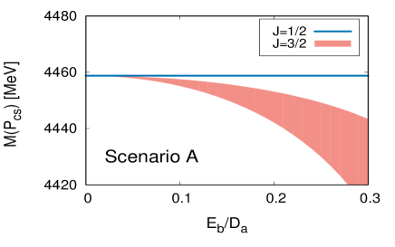
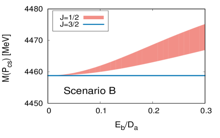
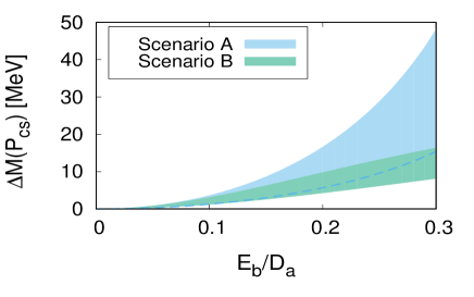
Figure 1: Masses and hyperfine splitting of the $J=\tfrac{1}{2}$ and $\tfrac{3}{2}$ molecular $P_{cs}$ pentaquarks. For $J=\tfrac{1}{2}$ ($\tfrac{3}{2}$) we include the coupled channel dynamics $\bar{D}\Xi_{c}^{\prime}$-$\bar{D}^{*}\Xi_{c}$ ($\bar{D}^{*}\Xi_{c}$-$\bar{D}\Xi_{c}^{*}$), which are expected to be ${\rm LO}$ effects in the EFT description. This description contains three independent couplings $C_{a}$, $D_{a}$, $E_{b}$, where the first one ($C_{a}$) is determined from the $P_{c}(4312)$ pentaquark and SU(3)-flavor symmetry. For the other two couplings we do as follows: scenario $A$ ($B$) assumes that the observed $P_{cs}$ pentaquark is the $J=\tfrac{1}{2}$ ($\tfrac{3}{2}$) configuration; then for a given $E_{b}/D_{a}$ ratio we determine $D_{a}$ from the $P_{cs}$ mass. Finally, we show the hyperfine splitting $\Delta M(P_{cs})=M(P_{cs},J=\tfrac{1}{2})-M(P_{cs},J=\tfrac{3}{2})$ in both scenarios.

5 Meson exchange saturation

The problem we have is that there are three couplings ($C_{a}$, $D_{a}$, $E_{b}$) of which we can only determine two ($C_{a}$ from the $P_{c}(4312)$ and $D_{a}$ or $E_{b}$ from the $P_{cs}(4459)$). Yet, if we use phenomenology it might be possible to find relations among these couplings and thus determine the three of them. In particular we will focus on light-meson saturation, i.e. the idea that the contact-range couplings of a given EFT are saturated by the exchange of light mesons Ecker et al. (1989); Epelbaum et al. (2002). Here we choose the novel saturation procedure of Ref. Peng et al. (2020), which we explain below.

Standard saturation maps the finite-range S-wave potential generated by the exchange of a light-meson, $V_{M}({\vec{q}\,}^{2})$ (with $\vec{q}=\vec{p}\,^{\prime}-\vec{p}$ the exchanged momentum, where for S-wave we can express the potential as a function of ${\vec{q}\,}^{2}$), into a contact-range coupling $C^{\rm sat}$ by taking the limit

$$C^{\rm sat\,(standard)}(\Lambda\sim m)\propto\lim_{\vec{q}^{2}\to 0}V_{M}(\vec{q}^{2})\,,$$ (23)

which is expected to work for $\Lambda$ close to the mass $m$ of the exchanged meson. However, if the potential vanishes in this limit, we will obtain $C^{\rm sat}=0$. For instance, the potentials

$$V_{M}=-g_{Y}^{2}\,\frac{1}{m^{2}+\vec{q}^{2}}\quad\mbox{and}\quad V_{M}^{\prime}=+g_{Y}^{2}\,\frac{\vec{q}^{2}}{m^{2}}\frac{1}{m^{2}+\vec{q}^{2}}\,,$$ (24)

generate exactly the same finite-range potential in r-space, namely the Yukawa potential

$$V_{M}^{(^{\prime})}(r)=-g_{Y}^{2}\frac{e^{-mr}}{4\pi r}\quad\mbox{for $r\neq 0$}\,,$$ (25)

where the difference between the two is a distribution

$$V_{M}^{\prime}(r)-V_{M}(r)=g_{Y}^{2}\,m\,\delta^{(3)}(m\,\vec{r})\,.$$ (26)

Of course, at this point we have to discuss the impact of form-factors, which modify the light-meson exchange potentials as follows

$$V_{M}^{(^{\prime})}(\vec{q};\Lambda_{M})=V_{M}^{(^{\prime})}(\vec{q})F_{M}^{2}(\vec{q},\Lambda_{M})\,,$$ (27)

where $F_{M}$ is the aforementioned form-factor (with the most used parametrizations being of the multipolar type) while $\Lambda_{M}$ is the form-factor cutoff, which should not be confused with the EFT cutoff $\Lambda$. For a local form-factor the resulting r-space potentials will be also local, and the Dirac-delta will acquire a finite-size:

$$\delta^{(3)}(m\,\vec{r})\to\delta_{F}^{(3)}(m\,\vec{r};\frac{m}{\Lambda_{M}})\,,$$ (28)

where $\delta_{F}^{(3)}$ represents a Dirac-delta that has been already smeared out by the form-factor. Yet, the characteristic scale $\Lambda_{M}$ of these finite-range effects is expected to be larger than the mass of the exchanged meson, i.e. $\Lambda_{M}>m$ (otherwise the effect of said exchanged light-meson will be washed out by the form factors). For instance, for the Bonn-B potential Machleidt et al. (1987) $\Lambda_{\sigma}=1.9-2.0\,{\rm GeV}$ and $\Lambda_{\rho/\omega}=1.85\,{\rm GeV}$ for the $M=\sigma$ and $\rho$/$\omega$ mesons, respectively, while for the CD-Bonn potential Machleidt (2001) we have $\Lambda_{\sigma}=2.5\,{\rm GeV}$, $\Lambda_{\rho}=1.31\,{\rm GeV}$ and $\Lambda_{\omega}=1.5\,{\rm GeV}$.

Thus for the range of cutoffs in which saturation is expected to work we have $(\Lambda\sim m)<\Lambda_{F}$, which implies that the previous Dirac-delta is unimportant: independently of whether the potential is derived from derivative interactions ($V_{M}^{\prime}$) or not ($V_{M}$), the potentials at $mr\sim 1$ will be similar and thus the saturation of the couplings should follow suit. That is, if the renormalization scale is similar to the exchanged meson mass, the potentials $V_{M}$ and $V_{M}^{\prime}$ are expected to lead to approximately the same saturated coupling. This is achieved with the convention

$$C^{\rm sat\,(new)}(\Lambda\sim m)\propto\frac{1}{m^{2}}\,\underset{{\vec{q}^{2}\to-m^{2}}}{\rm Res}V_{M}^{(^{\prime})}(\vec{q}^{2})\,,$$ (29)

i.e. by extracting the residue of the potential at $\vec{q}^{2}=-m^{2}$, which effectively recovers the expectations from the $mr\sim 1$ behavior of the potential. Ref. Peng et al. (2020) explicitly checked this method with the one-pion-exchange potential (with an arbitrary coupling strength) as a specific example. In Appendix B we include a detailed comparison between the standard saturation procedure of Ref. Epelbaum et al. (2002) and the one presented here for the particular case of the nucleon-nucleon system, which indicates that both saturation methods yield comparable results.

Now, if we consider the scalar meson $\sigma$, in the non-relativistic limit it generates a spin-independent potential which can contribute to the saturation of $C_{a}$ and $D_{a}$ (but not $C_{b}$ or $E_{b}$):

$$V_{S}(\vec{q}) = -\frac{g_{\sigma i}g_{\sigma j}}{m_{S}^{2}+{\vec{q}\,}^{2}}\,,$$ (30)

where $m_{S}$ the mass of the sigma meson and $g_{\sigma i}$ its coupling, and the indices $i,j=1,2,3$ referring to the $\bar{D}^{(*)}$, $\Xi_{c}^{(^{\prime}/*)}$ and $\Xi_{c}$, respectively. Independently of the saturation method we will obtain

$$F_{a}^{\rm sat(S)}(\Lambda\sim m_{S}) \propto -\frac{g_{\sigma i}g_{\sigma j}}{m_{S}^{2}}\,,$$ (31)

with $F_{a}=C_{a},D_{a}$ the generic name for the spin-independent couplings. The proportionality constant is in principle unknown, but we will assume it to be similar for all the couplings. We remind that saturation is expected to work for cutoffs close to the mass of the meson being exchanged, $\Lambda\sim m_{S}$ in this case.

The vector mesons ($\rho$ and $\omega$) generate a more complex potential which can be expanded in a multipole expansion similar to the one we have for electromagnetic interactions. There are electric- and magnetic-type components (indicated by the subscripts $a$ and $b$)

$$V_{V} = V_{Va}+V_{Vb}\,,$$ (32)

with

$$V_{Va} = +(1+\vec{\tau}_{1}\cdot\vec{\tau}_{2})\,\frac{g_{Vi}g_{Vj}}{m_{V}^{2}+{\vec{q}\,}^{2}}\,,$$ (33)

$$V_{Vb} = -(1+\vec{\tau}_{1}\cdot\vec{\tau}_{2})\,\frac{f_{Vi}f_{Vj}}{6M^{2}}\,\mathcal{O}_{L12}\,\frac{{\vec{q}\,}^{2}}{m_{V}^{2}+{\vec{q}\,}^{2}}+\dots\,,$$ (34)

and $O_{L12}=0$, $\vec{\sigma}_{L}\cdot\vec{\epsilon}_{L}$ or $\vec{\sigma}_{L}\cdot\vec{S}_{L}$ for $\bar{H}_{c}T$, $\bar{H}_{c}T_{c}$-$\bar{H}_{c}S_{c}$ and $\bar{H}_{c}S_{c}$, respectively, where the dots represent S-to-D-wave components (we assume they will not appreciably contribute to the saturation of the EFT couplings). In the vector-exchange potential the $i,j$ indices refer to the different hadrons involved, $g_{Vi}$ to the electric-type couplings, $f_{Vi}$ to the magnetic-like ones, $m_{V}$ to the vector meson mass and $M$ a typical hadronic mass scale. The $V_{Va}$ component contribute to the $C_{a}$ and $D_{a}$ couplings as

$$F_{a}^{\rm sat(V)}(\Lambda\sim m_{V}) \propto (1+\vec{\tau}_{1}\cdot\vec{\tau}_{2})\,\frac{g_{Vi}g_{Vj}}{m_{V}^{2}}\,,$$ (35)

where $F_{a}=C_{a}$, $D_{a}$, with no difference between the standard and modified saturation procedures, i.e. Eqs. (23) and  (29). For the $V_{Vb}$ component to contribute to the $C_{b}$ and $E_{b}$ couplings in a non-trivial way we have to use the modified saturation procedure of Ref. Peng et al. (2020) (i.e. Eq. (29)) in which case we obtain

$$F_{b}^{\rm sat(V)}(\Lambda\sim m_{V}) \propto (1+\vec{\tau}_{1}\cdot\vec{\tau}_{2})\,\frac{f_{Vi}f_{Vj}}{6M^{2}}\,,$$ (36)

where $F_{b}=C_{b},E_{b}$. Here we notice that with the standard saturation method we would have arrived to $C_{b}=E_{b}=0$. This is what happens for instance in Refs. Xiao et al. (2019a, b), which in principle consider the complete set of ${\rm LO}$ interactions we have here, i.e. Eqs. (6), (11) and (12), but set the $F_{b}$-type couplings to zero leading to pentaquark predictions without sizable hyperfine splittings. Yet, as we will see, from the point of view of phenomenology the choice of Refs. Xiao et al. (2019a, b) is completely justified: the size of the $F_{b}$-type of coupling is expected to be considerably smaller than the $F_{a}$-type, which prompts the approximation $F_{b}=0$. In contrast from the EFT point of view the inclusion of the $F_{b}$ couplings is justified in terms of power counting.

The only thing left is to determine the couplings: for the $\sigma$ we will use the linear-sigma model Gell-Mann and Levy (1960) and the quark model (as used in Ref. Riska and Brown (2001)), from which we get that the coupling of the sigma to the nucleon is $g_{\sigma NN}=\sqrt{2}M_{N}/f_{\pi}\sim 10.2$ (for the $f_{\pi}\simeq 132\,{\rm MeV}$ normalization). For the charmed mesons with only one light-quark we end up with $g_{\sigma 1}=g_{\sigma NN}/3\simeq 3.4$, while for the charmed baryons with two light-quarks we have $g_{\sigma 2}=g_{\sigma 3}=2\,g_{\sigma NN}/3\simeq 6.8$. We note that here we have assumed the same coupling of the sigma with the $q=u,d,s$ quarks, as happens for instance in the quark model of Ref. Vijande and Valcarce (2009), where we notice that this pattern can either arise from a singlet sigma (not necessarily a realistic assumption) or alternatively from a negligible coupling of the octet component of the sigma to the light quarks, see for instance Ref. Yan et al. (2021) for a more detailed discussion. In either case, this runs counter to the standard expectation that the strange and non-strange components of light mesons would decouple (owing to the OZI rule), leading in the case of the sigma to a vanishing coupling to the strange quark. However it has been argued that the OZI rule does not work so well in the $0^{++}$ sector Geiger and Isgur (1993); Lipkin and Zou (1996); Isgur and Thacker (2001); Meissner and Oller (2001), i.e. a non-singlet sigma might potentially have a non-negligible coupling with the strange quark. Besides, the singlet and octet mixing angle of the sigma might very well be far away from the angle decoupling strange and non-strange components Oller (2003). Yet, even though the sigma coupling to the strange quark might not be necessarily suppressed, it might not be as strong as with the light-quarks. This can generate SU(3)-flavor breaking effects which we will discuss later, where the naive expectation will be that the contribution of the sigma to the contact-range couplings will be weaker in the $\bar{D}\Xi_{c}^{{}^{\prime}}$ and $\bar{D}^{*}\Xi_{c}$ molecules than in the $\bar{D}\Sigma_{c}$ one. For further details we refer to the discussion around Eq. 73, where we notice that the previous expectation seems to be challenged by the experimental information currently available .

For the vector mesons, we have electric- and magnetic-like couplings, for which we will resort to Sakurai’s universality and vector meson dominance Sakurai (1960); Kawarabayashi and Suzuki (1966); Riazuddin and Fayyazuddin (1966), i.e. the mixing of the neutral vector mesons with the electromagnetic current, which can be encapsulated in the substitution rules Liu et al. (2021b); Peng et al. (2021)

$$\rho^{3}_{\mu}\to\frac{1}{\beta}\,\frac{e}{2g}\,A_{\mu}\quad\mbox{and}\quad\omega_{\mu}\to\frac{1}{\beta}\,\frac{e}{6g}\,A_{\mu}\,,$$ (37)

where $e$ is the proton charge, $g=m_{V}/2f_{\pi}\simeq 2.9$ the universal rho coupling constant (with $m_{V}$ the vector meson mass and $f_{\pi}\simeq 132\,{\rm MeV}$ the pion weak decay constant), $A_{\mu}$ the photon field, $\rho^{3}_{\mu}$ the neutral rho field (the superscript refers to the isospin index, $a=3$ for the neutral component), $\omega_{\mu}$ the omega field and $\mu$ a Lorentz index. The parameter $\beta$ indicates the degree of vector meson dominance: if the electromagnetic couplings of the heavy hadrons were to be completely dominated by the vector mesons, we will have $\beta=1$. Otherwise it will be $\beta<1$. Usually $\beta\simeq 0.9$ is estimated Isola et al. (2003); Liu and Oka (2012); Dong et al. (2020) (which can be traced back to the ratio of the couplings required for the $\rho\to\gamma\gamma$ and $\rho\to\pi\pi$ processes, i.e. $\sqrt{2}f_{\pi}/f_{\rho}\sim 0.9$). By applying these substitution rules to the interaction of the heavy hadrons with the vector mesons, we will get the electromagnetic interaction for the light quarks within the heavy hadrons and from this, we can determine the $g_{Vi}$ and $f_{Vi}$ couplings. In practical terms this means that $g_{Vi}$ and $f_{Vi}$ are proportional to the light-quark contribution of the electric charge and magnetic moments of the heavy hadrons, respectively. For the E0 couplings we get $g_{V1}=g_{V2}=g_{V3}=\beta g$. For the M1 couplings, we will first make the decomposition $f_{V}=\kappa_{V}g_{V}$ and use the choice $M=m_{N}$ for the mass scale with $m_{N}\simeq 940\,{\rm MeV}$ the nucleon mass. From this $\kappa_{V}=\frac{3}{2}(\mu_{u}/\mu_{\rm n.m.})$, with $\mu_{u}/\mu_{\rm n.m.}$ the magnetic moment of the u-quark within light-diquark pair inside the $\Xi_{c}^{+}$/$\Xi_{c}^{(^{\prime}/*)+}$ charmed baryon expressed in units of the nuclear magneton ($\mu_{\rm n.m.}$). If we make use of the quark model a second time, we obtain $\kappa_{V1}=\kappa_{V2}=\frac{3}{2}\mu_{u}/\mu_{\rm n.m.}\simeq 2.9$ for the charmed antimeson and sextet strange charmed baryon. For the antitriplet charmed baryon we have instead $\kappa_{V3}=0$, which is a consequence of the two light-quarks within the $\Xi_{c}$ baryon being in a spin-0 configuration. The $E_{b}$ coupling involves a M1 antitriplet to sextet transition for which $\kappa_{V}(\bar{3}\to 6)=\frac{3}{2}\,\mu(\bar{3}\to 6)/\mu_{\rm n.m.}=\frac{3}{2}(\mu_{u}/\mu_{\rm n.m.})\simeq 2.9$, where $\mu(\bar{3}\to 6)$ refers to the u-quark magnetic moment in the $\bar{3}\to 6$ light-diquark transition  within $\Xi_{c}^{+}\to\Xi_{c}^{(^{\prime},*)+}$.

With the previous couplings and setting $m_{S}\simeq 550\,{\rm MeV}$ and $m_{V}=(m_{\rho}+m_{m_{\omega}})/2\simeq 775\,{\rm MeV}$, we arrive to the ratios:

$$\frac{C_{b}^{\rm sat}}{C_{a}^{\rm sat}}{\Big{|}}_{\Lambda\sim(m_{S}-m_{V})} \sim 0.20\,,$$ (38)

$$\frac{D_{a}^{\rm sat}}{C_{a}^{\rm sat}}{\Big{|}}_{\Lambda\sim(m_{S}-m_{V})} \sim 1.00\,,$$ (39)

$$\frac{E_{b}^{\rm sat}}{D_{a}^{\rm sat}}{\Big{|}}_{\Lambda\sim(m_{S}-m_{V})} \sim 0.20\,.$$ (40)

The first one of these ratios was checked in Ref. Liu et al. (2021b), where it was respected at the $30\%$ level. If we determine $C_{a}$ and $C_{b}$ as in Ref. Liu et al. (2019), we obtain $|C_{b}/C_{a}|=0.16$ for $\Lambda=0.75\,{\rm GeV}$, which reproduces the absolute magnitude of Eq. (38) at the $25\%$ level. However we note that in Ref. Liu et al. (2019) the sign of $C_{b}$ depends on which are the spin of the $P_{c}(4440)$ and $P_{c}(4457)$ pentaquarks: the sign is correctly reproduced if the $P_{c}(4457)$ is $J=\tfrac{1}{2}$. The second one ($C_{a}=D_{a}$) appears for instance in Ref. Wu et al. (2010), which predicted the $P_{cs}$, and Refs. Wu et al. (2011); Xiao et al. (2019b); Shen et al. (2019) as a consequence of the universality of the vector meson coupling. The recent work of Ref. Wang et al. (2020) uses the chiral quark model to guess the contact-range couplings, leading to $C_{a}\simeq D_{a}$ too. The third relation has not been previously used, as $E_{b}$ is usually set to zero (e.g. Ref. Xiao et al. (2019b), where their $E_{b}$ equivalent is called $\hat{\mu}_{24}$). Finally it is worth noticing the following

$$\frac{C_{b}^{\rm sat}}{C_{a}^{\rm sat}}\sim\frac{E_{b}^{\rm sat}}{D_{a}^{\rm sat}}\,,$$ (41)

where this relation actually does not depend so much on saturation being correct or accurate, but rather on the fact that the light-meson exchange potentials are identical under the approximations we have made. In the following lines we will explore the consequences of this relation.

6 Accidental symmetry in the pentaquark potential

Light-meson exchange actually suggests a very interesting relation between the $P_{c}(4440)$, $P_{c}(4457)$ and the two spin states of $\bar{D}^{*}\Xi_{c}$. The S-wave light-meson exchange potential in the $\bar{H}_{c}S_{c}$ system is

$$V_{\rm OBE}(\bar{H}_{c}S_{c})=V_{a}+V_{b}\,\vec{\sigma}_{L}\cdot\vec{S}_{L}\,,$$ (42)

which for the $J=\tfrac{1}{2}$, $\tfrac{3}{2}$ $\bar{D}^{*}\Sigma_{c}$ systems reads

$$V_{\rm OBE}(\bar{D}^{*}\Sigma_{c},\tfrac{1}{2}) = V_{a}-\frac{4}{3}V_{b}\,,$$ (43)

$$V_{\rm OBE}(\bar{D}^{*}\Sigma_{c},\tfrac{3}{2}) = V_{a}+\frac{2}{3}V_{b}\,,$$ (44)

from which we expect the hyperfine splitting to be proportional to

$$M(\bar{D}^{*}\Sigma_{c},\tfrac{3}{2})-M(\bar{D}^{*}\Sigma_{c},\tfrac{1}{2})\propto 2V_{b}\,.$$ (45)

In comparison for the coupled $\bar{H}_{c}T_{c}$-$\bar{H}_{c}S_{c}$ system, the corresponding potential reads

$$V_{\rm OBE}(\bar{H}_{c}T_{c},\bar{H}_{c}S_{c})=\begin{pmatrix}W_{a}&W_{b}\,\vec{\sigma}_{L}\cdot\vec{\epsilon}_{L}\\ W_{b}\,\vec{\sigma}_{L}\cdot\vec{\epsilon}_{L}&V_{a}+V_{b}\,\vec{\sigma}_{L}\cdot\vec{S}_{L}\\ \end{pmatrix}$$ (46)

where if we consider vector meson exchange, vector meson dominance, the quark model relations for the charmed baryon magnetic moments and SU(3) symmetric sigma exchange, we will have

$$V_{a}\simeq W_{a}\qquad\mbox{and}\quad V_{b}\simeq W_{b}\,.$$ (47)

This will receive small corrections from $\eta$-exchange (that work in the direction of making $|W_{b}|>|V_{b}|$), which we will ignore as they are small. Now, in the limit where the $\bar{D}\Xi_{c}^{\prime}$-$\bar{D}\Xi_{c}$ and $\bar{D}\Xi_{c}^{*}$-$\bar{D}^{*}\Xi_{c}$ thresholds are degenerate and have the same mass, there will be two eigenvalues for this potential, which correspond to the linear combinations

$$|\bar{D}^{*}\Xi_{c}(J=\tfrac{1}{2})(\pm)\rangle = \frac{1}{\sqrt{2}}\left[|\bar{D}\Xi_{c}^{\prime}\rangle\pm|\bar{D}\Xi_{c}^{*}\rangle\right]\,,$$ (48)

$$|\bar{D}^{*}\Xi_{c}(J=\tfrac{3}{2})(\pm)\rangle = \frac{1}{\sqrt{2}}\left[|\bar{D}^{*}\Xi_{c}\rangle\pm|\bar{D}\Xi_{c}^{*}\rangle\right]\,,$$ (49)

with potential eigenvalues

$$V_{\rm OBE}(J=\tfrac{1}{2},\tfrac{3}{2},\pm)=\frac{1}{2}(W_{a}+V_{a})\pm W_{b}\simeq V_{a}\pm V_{b}\,.$$ (50)

In particular, in this limit the hyperfine splitting between the “$\pm$ states” will be

$$M(\bar{D}^{*}\Xi_{c},+)-M(\bar{D}^{*}\Xi_{c},-)\propto 2W_{b}\simeq 2V_{b}\,,$$ (51)

that is, expected to be similar to the hyperfine splitting between the $J=\tfrac{1}{2}$ and $\tfrac{3}{2}$ $\bar{D}^{*}\Sigma_{c}$ states.

Of course, this accidental symmetry in the potential will be broken by the fact that there is a mass gap between the involved coupled channels. The effect of this mass gap will be to decrease the hyperfine splitting and to force the “$\pm$” sign in Eq. (50) as to make the state corresponding to the lower threshold the most attractive configuration. If we compare the characteristic momentum scale of the coupled channel exchange potential (i.e. the vector meson mass $m_{V}$) and the momentum scale of the coupled channel dynamics ($\Lambda_{CC}=\sqrt{2\mu\Delta_{CC}}\simeq 266$ and $279\,{\rm MeV}$), the ratio is $0.34$ and $0.36$ for the $\bar{D}\Xi_{c}^{\prime}$ and $\bar{D}\Xi_{c}^{*}$ channels, respectively. Together they add to $0.70$, i.e. we expect the hyperfine splittings to be about $30\%$ of the expected value were not to be a mass gap. For the $J=\tfrac{1}{2}$ ($\tfrac{3}{2}$) configuration, the $\bar{D}^{*}\Xi_{c}$ threshold is heavier (lighter) than the $\bar{D}\Xi_{c}^{\prime}$ ($\bar{D}\Xi_{c}^{*}$) one, which forces the most repulsive (attractive) sign configuration in Eq. (51).

$$M(\bar{D}^{*}\Xi_{c},\tfrac{1}{2})-M(\bar{D}^{*}\Xi_{c},\tfrac{3}{2}) \propto 2|W_{b}|\left(1-\sum_{CC}\mathcal{O}(\frac{\Lambda_{CC}}{m})\right)$$ (52)

$$\simeq 2|V_{b}|\left(1-\sum_{CC}\mathcal{O}(\frac{\Lambda_{CC}}{m})\right)\,.$$

As a consequence, if the previous approximations hold, the hyperfine splitting of the two $\bar{D}^{*}\Xi_{c}$ pentaquarks will be similar to the one of the two $\bar{D}^{*}\Sigma_{c}$ pentaquarks, i.e.

$$|M(\bar{D}^{*}\Xi_{c},\tfrac{1}{2})-M(\bar{D}^{*}\Xi_{c},\tfrac{3}{2})|\simeq 17\,{\rm MeV}\,.$$ (53)

However if the effect is to be reduced by a $70\%$, as suggested by the scale comparison, we will end up with a $5.1\,{\rm MeV}$ splitting. Though the sign of the hyperfine splitting might be protected owing to power counting and the nature of the coupled channel dynamics, its size will be diminished owing to the finite mass gaps between the channels. Besides, the uncertainties in the couplings of the light-meson exchange potential are also large. In the following we will see how this expected effect holds when compared with different error sources.

For doing the explicit calculations we first obtain the $C_{a}$ and $C_{b}$ couplings from the masses of the $P_{c}(4440)$ and $P_{c}(4457)$ pentaquarks, i.e. the calculation of Ref. Liu et al. (2019), where we notice that for the hyperfine splitting it does not matter which spin is each pentaquark , resulting in $C_{a}=-2.52\,(-0.85)\,{\rm fm}^{2}$, $C_{b}=\pm 0.54\,(0.11)\,{\rm fm}^{2}$ for $\Lambda=0.5\,(1.0)\,{\rm GeV}$. Then we consider the phenomenological potential symmetry of Eq. (47) as applied to the contact-range couplings (i.e. $C_{a}=D_{a}$, $C_{b}=E_{b}$), from which we get:

$$M(P_{cs},\tfrac{1}{2}) = 4464.5-1.1i\,(4464.4-1.3i)\,{\rm MeV}\,,$$ (54)

$$M(P_{cs},\tfrac{3}{2}) = 4459.9(4459.7)\,{\rm MeV}\,,$$ (55)

for $\Lambda=0.5\,(1.0)\,{\rm GeV}$, with the hyperfine splitting

$$\Delta M(P_{cs})=4.6\,(4.7)\,{\rm MeV}\,,$$ (56)

which indeed indicates a reduction of the coupled channel effects owing to the finite mass gap between the channels, and where from now on we define

$$\Delta M(P_{cs})=M(\tfrac{1}{2})-M(\tfrac{3}{2})\,.$$ (57)

Yet, even if this accidental symmetry is greatly reduced in the hyperfine splittings, it is worth noticing that the predictions we obtain from using the effective $C_{a}$ and $C_{b}$ couplings describing the $P_{c}(4440)$ and $P_{c}(4457)$ pentaquarks are basically compatible with the experimental mass of the observed $P_{cs}$ pentaquark.

7 The hyperfine splitting

Assumptions:	$J$	$M(J)$	$M(J=1/2)-M(J=3/2)$
EFT A: $\,\,{E_{b}}/{D_{a}}\sim{Q}/{M}$ and	${1}/{2}$	$4458.8$ (Input)	$21.5\,(11.6-35.4)$
$D_{a}$ from $P_{cs}(4459)$ as $J=\frac{1}{2}$	${3}/{2}$	$4437.3\,(4423.3-4447.2)$
EFT B: $\,\,{E_{b}}/{D_{a}}\sim{Q}/{M}$ and	${1}/{2}$	$4469.5\,(4465.7-4473.4)$	$10.7\,(6.9-14.6)$
$D_{a}$ from $P_{cs}(4459)$ as $J=\frac{3}{2}$	${3}/{2}$	$4458.8$ (Input)
EFT+RG A: $\,\,{E_{b}}/{D_{a}}\sim\mathcal{F}(Q/\Lambda)\,{Q}/{M}$	${1}/{2}$	$4458.8$ (Input)	$30.6\,(27.4-40.4)$
and $D_{a}$ from $P_{cs}(4459)$ as $J=\frac{1}{2}$	${3}/{2}$	$4428.1\,(4417.7-4431.5)$
EFT+RG B: $\,\,{E_{b}}/{D_{a}}\sim\mathcal{F}(Q/\Lambda)\,{Q}/{M}$	${1}/{2}$	$4471.4\,(4470.7-4471.7)$	$12.6\,(11.9-12.9)$
and $D_{a}$ from $P_{cs}(4459)$ as $J=\frac{3}{2}$	${3}/{2}$	$4458.8$ (Input)
Accidental: $\,\,C_{a}\sim D_{a}$, $C_{b}\sim E_{b}$	${1}/{2}$	$4464.5\,(4464.40-4464.5)$	$4.7\,(4.6-4.7)$
and $C_{a}$, $C_{b}$ from $P_{c}(4440/4457)$	${3}/{2}$	$4459.8\,(4459.7-4459.9)$
Saturation I: $\,\,C_{a}\sim D_{a}$ and	${1}/{2}$	$4473.1\,(4471.1-4475.3)$	$14.3\,(12.7-16.5)$
$E_{b}$ from $P_{cs}(4459)$ as $J=\tfrac{3}{2}$	${3}/{2}$	$4458.8$ (Input)
Saturation II:	${1}/{2}$	$4469.6\,(4469.2-4470.1)$	$5.3\,(3.4-8.8)$
$C_{a}\sim D_{a}$ and $E_{b}\sim 0.2D_{a}$	${3}/{2}$	$4464.3\,(4461.3-4466.6)$
Two-peak solution:	${1}/{2}$	$4467.8$ (Input)	$12.9$ (Input)
$C_{a}=0.90D_{a}$ and $E_{b}=0.28D_{a}$	${3}/{2}$	$4454.9$ (Input)

Table 1: Expected masses and hyperfine splitting (in units of ${\rm MeV}$) of the $J=\tfrac{1}{2}$ $\bar{D}\Xi_{c}^{\prime}$-$\bar{D}^{*}\Xi_{c}$ and $J=\tfrac{3}{2}$ $\bar{D}^{*}\Xi_{c}$-$\bar{D}\Xi_{c}^{*}$ pentaquarks with the different assumptions considered in this work. They include power counting estimations from EFT (“EFT A & B”), the RG-improved EFT (“EFT+RGA A&B”, where RG stands for “renormalization group”), the accidental symmetry of the scalar and vector meson exchange potentials between the $P_{c}(4440/4457)$ and the new $P_{cs}(4459)$ (“Accidental”), and the saturation relations Eqs. (39) and (40) (“Saturation I & II”). The central values correspond to $\Lambda=0.75$ ${\rm GeV}$, while the spread to $\Lambda=0.5-1.0$ ${\rm GeV}$. At the end (“Two-peak solution”) we compare with the two-peak fit of Ref. Aaij et al. (2020), from which an hyperfine splitting of $12.9\pm 4.6\,{\rm MeV}$ is expected. If this figure turns out to be confirmed by future experimental studies, this will discard the “EFT A”, “EFT+RGA A”, “Accidental” and “Saturation II” estimations.

Now we will analyze the possible size of the hyperfine splittings with the (admittedly approximate) information we have derived from light-meson exchange saturation. We begin with the simplest of the relations, that is:

$$\frac{D_{a}}{C_{a}}\sim 1\,,$$ (58)

and determine $C_{a}$ from reproducing the $P_{c}(4312)$ pentaquark, which yields $C_{a}=-1.19$ ($-(2.17-0.80)$) ${\rm fm}^{2}$ for $\Lambda=0.75$ ($0.5-1.0$) $\rm GeV$, where we will use a central value of the cutoff close to the expected scale at which saturation works (i.e. $\Lambda\sim m_{V}$), while we will still consider the $0.5-1.0\,{\rm GeV}$ cutoff range for estimating the regulator uncertainties. If we set $E_{b}=0$, it will lead to

$$M(P_{cs},J=\tfrac{1}{2},\tfrac{3}{2})=4467.5\,(4466.9-4468.1)\,{\rm MeV}\,,$$ (59)

that is, we obtain two degenerate $P_{cs}$ pentaquarks. If we allow for $E_{b}\neq 0$ we can effectively fit one of the pentaquarks to the experimental mass. We obtain .:

$$M(P_{cs},\tfrac{1}{2}) = 4473.1(4471.1-4475.3)\,{\rm MeV}\,,$$ (60)

$$M(P_{cs},\tfrac{3}{2}) = 4458.8\,{\rm MeV}\,,$$ (61)

where it should be noticed that scenario B is automatically chosen, as for $C_{a}/D_{a}\sim 1$ the mass of the $P_{cs}$ pentaquark can only be reproduced if $J=\tfrac{3}{2}$. The hyperfine splitting will be

$$\Delta M(P_{cs})=14.3\,(12.7-16.5)\,{\rm MeV}\,,$$ (62)

which is definitely larger than the estimation from the phenomenological symmetry in the pentaquark potential. The ratio $E_{b}/D_{b}=0.34\,(0.24-0.53)$ will also be larger than the expectation from saturation, Eq. (40).

Alternatively we can assume that the saturation relations in Eqs. (39) and (40) both hold, in which case the masses of the two $P_{cs}$’s are

$$M(P_{cs},\tfrac{1}{2}) = 4469.6\,(4469.2-4470.1)\,{\rm MeV}\,,$$ (63)

$$M(P_{cs},\tfrac{3}{2}) = 4464.3\,(4461.3-4466.6)\,{\rm MeV}\,,$$ (64)

and the hyperfine splitting is

$$\Delta M(P_{cs})=5.3\,(3.4-8.8)\,{\rm MeV}\,,$$ (65)

which is closer to the one we derived from the phenomenological symmetry, i.e. Eq. (56).

Now there are a series of (potentially large) uncertainties related to the previous relations. The most obvious one is the existence of SU(3)-breaking corrections between the coupling in the $\bar{D}\Sigma_{c}$ (strangeness $S=0$) and the $\bar{D}\Xi_{c}^{\prime}$, $\bar{D}\Xi_{c}^{*}$ (strangeness $S=-1$) systems, i.e. between the $P_{c}(4312)$ and $P_{cs}^{\prime}$, $P_{cs}^{*}$ pentaquarks. Their couplings, which are identical if SU(3)-flavor symmetry is exactly preserved, will differ by a correction

$$C_{a}(P_{cs}^{(^{\prime}/*)})=C_{a}(P_{c})+\delta C_{a}^{\not{F}}\,.$$ (66)

where $\delta C_{a}^{\not{F}}$ indicates the correction to the $C_{a}$ coupling. From a comparison with the pion and kaon weak decay constants, $f_{\pi}\simeq 130\,{\rm MeV}$ and $f_{K}\simeq 160\,{\rm MeV}$, we expect the size of the SU(3)-breaking effects to be of the order of

$$\frac{\delta C_{a}^{\not{F}}}{C_{a}}\sim\left(\frac{f_{K}-f_{\pi}}{f_{\pi}}\right)\sim 0.23\,.$$ (67)

Alternatively, we can consider this problem from the point of view of chiral symmetry , in which the $C_{a}$ coupling can be decomposed into quark-mass independent and quark-mass dependent pieces Petschauer et al. (2020): the quark-mass dependent piece comes from terms in the Lagrangian where the quark-mass matrix is inserted between the hadron fields, with these terms expected to be subleading (as in this case we are expanding around the massless quark limit). This quark-mass dependence can be translated into a quadratic dependence on the mass of the pseudoscalar Nambu-Goldstone bosons, which can be schematically written as

$$C_{a}(P_{c}) = C_{a}^{[0,0]}+C_{a}^{[1,0]}\,\frac{m_{\pi}^{2}}{\Lambda_{\chi}^{2}}+C_{a}^{[0,1]}\,\frac{m_{\pi}^{2}}{\Lambda_{\chi}^{2}}+\dots\,,$$ (68)

$$C_{a}(P_{cs}^{(^{\prime}/*)}) = C_{a}^{[0,0]}+C_{a}^{[1,0]}\,\frac{m_{\pi}^{2}}{\Lambda_{\chi}^{2}}+C_{a}^{[0,1]}\,\frac{m_{K}^{2}}{\Lambda_{\chi}^{2}}+\dots\,,$$ (69)

where $C^{[n,m]}$ indicates $n$ ($m$) insertions of the quark mass matrix between the charmed antimeson (baryon) fields, $m_{\pi}$ and $m_{K}$ are the pion and kaon masses and $\Lambda_{\chi}\sim 1\,{\rm GeV}$ is the chiral symmetry breaking scale. Rearranging the terms, the difference can be rewritten in terms of a chiral symmetry breaking ($\chi SB$) correction, which takes the form

$$C_{a}(P_{cs}^{(^{\prime}/*)})=C_{a}(P_{c})+\delta C_{a}^{\chi SB}\,.$$ (70)

From the arguments about quark-mass dependence shown above, the size of this correction is expected to be of the order

$$\frac{\delta C_{a}^{\chi SB}}{C_{a}}\sim\left(\frac{m_{K}^{2}-m_{\pi}^{2}}{\Lambda_{\chi}^{2}}\right)\sim 0.23\,,$$ (71)

where it is interesting to notice that its size is identical to the previous estimation based on $f_{\pi}$ and $f_{K}$. The experience in the light-baryon sector suggests breakings larger than the previous estimation Haidenbauer et al. (2015), where repulsion increases with the number of strange quarks. The recent discovery of the $Z_{cs}$ Ablikim et al. (2021) allows for a comparison of the couplings required to reproduce the $Z_{c}$/$Z_{c}^{*}$ Albaladejo et al. (2016) and $Z_{cs}$ Yang et al. (2021) as virtual states, with attraction apparently increasing with the strange quark content (though the uncertainties are large).

Independently of the derivation, if SU(3)-breaking corrections reach a certain level they would lead to unbound $\bar{D}\Xi_{c}^{\prime}$ and $\bar{D}\Xi_{c}^{*}$ systems. In particular this will happen for

$$|C_{a}(P_{cs}^{\prime})|\leq 0.65\,(0.52-0.70)\,|C_{a}(P_{c})|\,,$$ (72)

for $\Lambda=0.75(0.5-1.0)\,{\rm GeV}$, where we indicate which pentaquark we are referring to in the parentheses. In this regard the previous $20\%$ estimations indicate that the SU(3)-symmetry partner of the $P_{c}(4312)$ pentaquark is still likely to bind. The eventual observation of a $\bar{D}\Xi_{c}^{\prime}$ molecular pentaquark could bring light to this issue.

A significant effect which might influence the size of SU(3)-flavor breaking corrections is the nature of sigma meson exchange: if the sigma were not to couple with the strange meson, saturation will suggest

$$\frac{C_{a}^{\rm sat}(P_{cs}^{\prime})}{C_{a}^{\rm sat}(P_{c})}\sim 0.62\,,$$ (73)

which is in the limit between binding and not binding for $P_{cs}^{\prime}$ (though in the no-binding case, the $P_{cs}^{\prime}$ pentaquark might still survive as a virtual state). Additionally, in this scenario from saturation we will expect

$$\frac{D_{a}}{C_{a}(P_{cs}^{\prime})}\sim 1.0\quad\mbox{and}\quad\frac{E_{b}}{D_{a}}\sim 0.33\,,$$ (74)

which would imply that the $P_{cs}$ could also very well be close to not binding (except for the increase in the relative strength of $E_{b}$, which would help in the $J=\tfrac{3}{2}$ configuration). With these coupling ratios, the masses of the molecular $P_{cs}$ pentaquarks would be

$$M(P_{cs},\tfrac{1}{2}) = 4478.0\,(4476.4-4478.1)\,{\rm MeV}\,,$$ (75)

$$M(P_{cs},\tfrac{3}{2}) = 4477.7\,(4476.7-4478.0)\,{\rm MeV}\,,$$ (76)

with the $J=\tfrac{1}{2}$ state in the second Riemann sheet with respect to the $D^{*}\Xi_{c}$ threshold (i.e. it is a shallow virtual state / resonance). That is, only the $J=\tfrac{3}{2}$ state is an actual bound state. In this later case the hyperfine splitting is compatible with zero and can even change signs as the $J=\tfrac{1}{2}$ is allowed to be a virtual state. However this large SU(3)-breaking in the direction of making the $\bar{D}^{*}\Xi_{c}$ less bound does not reproduce the experimental mass of the $P_{cs}$ pentaquark (unless we allow for $E_{b}/D_{a}\sim 1.23$, which is a considerable deviation from the saturation relations and would lead to a hyperfine splitting of $50.2$ $\rm MeV$). Thus it is unlikely that SU(3)-breaking would be as large as in Eq. (73), at least if its effect is to reduce attraction in the $\bar{D}\Xi^{\prime}$ system.

Finally, it is possible to make a comparison with the two-peak fit included in Ref. Aaij et al. (2020), which leads to two $P_{cs}$ pentaquarks with masses $4454.9\pm 2.7\,{\rm MeV}$ and $4467.8\pm 3.7\,{\rm MeV}$, respectively. Concrete calculations assuming that the lighter (heavier) $P_{cs}$ is a $J=\tfrac{3}{2}$ ($\tfrac{1}{2}$) $\bar{D}^{*}\Sigma_{c}$ molecule yield $D_{a}=-1.31$ $(-(2.59-0.86))\,{\rm fm^{2}}$ and $|E_{b}|=0.36$ $(0.95-0.19)\,{\rm fm}^{2}$ for $\Lambda=0.75(0.5-1.0)\,{\rm GeV}$. This determination of the couplings, together with the previous determination of $C_{a}$ from the $P_{c}(4312)$, provide the ratios

$$\frac{D_{a}}{C_{a}} = 1.11\,(1.19-1.07)\,,$$ (77)

$$\frac{E_{b}}{D_{a}} = 0.28\,(0.37-0.22)\,,$$ (78)

where the central value and the spreads correspond to $\Lambda=0.75\,(0.5-1.0)\,{\rm GeV}$, as usual. If the two-peak fit ends up being confirmed in future studies, the previous indicates a bit more attraction than expected for the $D_{a}$ coupling (but compatible with the errors we would expect for a phenomenological determination of the $D_{a}/C_{a}$ ratio) and that the size of $E_{b}$ seems to be underestimated by the phenomenological arguments we provide (yet compatible with the power counting estimates we proposed).

We summarize the different estimations we have considered along this work in Table 1. These indicate that, though it is not possible to determine the hyperfine splitting accurately from theory alone, power counting arguments and phenomenological approximations suggest it might be in the $5-15\,{\rm MeV}$ range (i.e. compatible with the two-peak fit in Aaij et al. (2020)), with the $J=3/2$ pentaquark being the lighter state. For comparison, Refs. Wu et al. (2010, 2011) predict degenerate $P_{cs}$ pentaquarks. Meanwhile, a recent calculation in the one-boson-exchange model generates a $\Delta M(P_{cs})=(2.4-20.0)\,{\rm MeV}$ splitting, which also comes from the $\bar{D}\Xi_{c}^{\prime}$-$\bar{D}^{*}\Xi_{c}$ and $\bar{D}^{*}\Xi_{c}$-$\bar{D}\Xi_{c}^{*}$ coupled channel dynamics Zhu et al. (2021). In contrast Ref. Wang et al. (2020) obtains $\Delta M(P_{cs})=-6.0\,{\rm MeV}$ from two-pion-exchange (TPE). This is interesting as the naive expectation would be that TPE is of order $(Q/M)^{2}$ in the EFT expansion and we might expect it to play a minor role. Thus, the role of TPE might indeed deserve further attention in the future. However there is the practical limitation that this calculation will also require $(Q/M)^{2}$ corrections to the contact-range potential, i.e. more unknown parameters.

Regarding which is the spin of the $P_{cs}$ pentaquark, from the different predictions in Table 1 it seems that the $J=\tfrac{3}{2}$ $\bar{D}\Xi_{c}^{*}$ configuration might provide a better match to its experimental mass, though uncertainties are too large to draw definite conclusions. It is also important to stress that the experimental determination of resonance masses usually relies in using the Breit-Wigner parametrization. Other parametrizations might yield different masses, as happened with the $P_{c}(4312)$ Fernández-Ramírez et al. (2019), the $Z_{c}(3900)$ / $Z_{c}(4020)$ Albaladejo et al. (2016), and the $Z_{cs}(3985)$ Yang et al. (2021). Thus the mass of a molecular $P_{cs}$ might not coincide with the experimental determination of Ref.  Aaij et al. (2020).

8 Decay into $J/\psi\Lambda$

It is interesting to notice that the observation of the $P_{cs}(4459)$ in the $J/\psi\Lambda$ channel might provide further circumstantial evidence of its spin. If we decompose the $J=\tfrac{1}{2}$, $\tfrac{3}{2}$ $\bar{D}^{*}\Xi_{c}$ system into its heavy- and light-quark spin components, we find

$$|\bar{D}^{*}\Xi_{c}(J=\tfrac{1}{2})\rangle = \left(\frac{\sqrt{3}}{2}0_{H}+\frac{1}{2}1_{H}\right)\otimes{\frac{1}{2}}_{L}\,,$$ (79)

$$|\bar{D}^{*}\Xi_{c}(J=\tfrac{3}{2})\rangle = 1_{H}\otimes{\frac{1}{2}}_{L}\,,$$ (80)

which is to be compared with

$$|J/\psi\Lambda\rangle=1_{H}\otimes{\frac{1}{2}}_{L}\,,$$ (81)

where $S_{H}$ and $S_{L}$ refer to the heavy- and light-quarks spin. If the decay preserves HQSS Sakai et al. (2019) the expect the following relation between matrix elements:

$$\langle J/\psi\Lambda|H|\bar{D}^{*}\Xi_{c}(J=\tfrac{1}{2})\rangle=\frac{1}{2}\,\langle J/\psi\Lambda|H|\bar{D}^{*}\Xi_{c}(J=\tfrac{3}{2})\rangle\,,$$

which for degenerate $\bar{D}^{*}\Xi_{c}$ states implies that the partial decay widths of the $J=\tfrac{1}{2}$ and $\tfrac{3}{2}$ configurations will show a $1\,:\,4$ ratio. In fact phenomenological calculations seems to support these ratios, with Ref. Xiao et al. (2019b) giving a $1\,:\,1.78$ ratio for the amplitudes / couplings and Ref. Xiao et al. (2021) yielding $1\,:\,4.35$ for the partial decay widths. Of course, this does not determine the spin of the $P_{cs}(4459)$, but nonetheless indicates that, ceteris paribus, the probability of discovering the $J=\tfrac{3}{2}$ molecule in the $J/\psi\Lambda$ invariant mass distribution might be larger than for its $J=\tfrac{1}{2}$ partner. But this conclusion is dependent on the production rates from the $\Xi_{b}$ decays, which have been recently investigated in Ref. Wu et al. (2021), suggesting that the production rate of a $J=\tfrac{3}{2}$ $\bar{D}^{*}\Xi_{c}$ pentaquark would be 4.9 times the one for its $J=\tfrac{1}{2}$ partner. Ideally, it would be possible to adapt the methods of Refs. Du et al. (2020, 2021) (originally formulated for the three $P_{c}$ pentaquarks) to analyze the invariant mass distribution data of the new $P_{cs}$.

9 Conclusions

The $P_{cs}(4459)$ is the latest piece of the pentaquark puzzle. Its closeness to the $\bar{D}^{*}\Xi_{c}$ threshold suggests that it might be a bound state of these hadrons. Then the question is what is the connection of the $P_{cs}(4459)$ with the well-known $P_{c}(4312)$, $P_{c}(4440)$ and $P_{c}(4457)$ in the molecular hypothesis. At first sight the answer is unclear: the $\bar{D}^{*}\Xi_{c}$ system is not directly connected by SU(3)-flavor and HQSS with the $\bar{D}\Sigma_{c}$ and $\bar{D}\Sigma_{c}^{*}$ systems, which are the usual molecular interpretations of the three $P_{c}$ pentaquarks. However if we resort to phenomenological arguments then we can bridge the gap between the new $P_{cs}$ and the previous $P_{c}$’s, resulting in a coherent description of these four pentaquarks. From vector meson dominance and the quark model, we point out a possible accidental symmetry between the potentials in the $P_{c}$ and $P_{cs}$ sectors, though owing to its phenomenological nature large deviations are to be expected.

There are two possible spin configurations for a molecular $P_{cs}$, which in principle should be degenerate. In this regard the explicit inclusion of the $\bar{D}\Xi_{c}^{\prime}$-$\bar{D}^{*}\Xi_{c}$ and $\bar{D}^{*}\Xi_{c}$-$\bar{D}\Xi_{c}^{*}$ coupled channel dynamics, which is required by power counting arguments, breaks this degeneracy and thus might have important implications for spectroscopy. This mechanism generates a sizable hyperfine splitting which we estimate to be in the $5-15\,{\rm MeV}$ range. Incidentally, this estimation is in line with the proposed two-peak solution in Aaij et al. (2020).

In general the predicted mass of the $J=\tfrac{3}{2}$ $P_{cs}$ pentaquark are closer to its experimental value than its $J=\tfrac{1}{2}$ partner, which might be interpreted as favoring the former spin assignment. But theoretical errors in the masses make it unpractical to determine the spin of the new pentaquark from spectroscopy alone. In this regard, the partial decay widths of the two spin configurations to $J/\psi\Lambda$, where the $P_{cs}$ have been discovered, approximately differ by a factor of four, making the $J=\tfrac{3}{2}$ configuration considerably easier to detect in this channel. Of course this is only true provided all other effects are similar. Independently of their spin, the existence of two possible $\bar{D}^{*}\Xi_{c}$ molecules tends to hold up well within the expected uncertainties of a phenomenological approach. As happened with the original $P_{c}(4450)$, future experiments could further determine whether there are really two $\bar{D}^{*}\Xi_{c}$ states and which is their mass difference.

Appendix A Power counting arguments with running coupling constants

In this work we have made use of power counting estimations of the size of the contact-range couplings appearing in the EFT description of the molecular pentaquarks. However the contact-range couplings are cutoff dependent and the aforementioned estimations were originally formulated for the renormalized couplings van Kolck (1999), the definition of which is scheme dependent. Yet, it has been argued that these estimations do indeed apply to running couplings if the cutoff is sufficiently soft Valderrama (2016); Epelbaum et al. (2017). But the previous arguments are qualitative in nature: here we will see how to modify dimensional estimations in a quantitative manner for their use with running couplings. This will be particularly useful for the dimensional estimation of the ratio of the $D_{a}$ and $E_{b}$ coupling constant employed in Sect. 4 (check Eq. (17)).

The easiest example will be a contact-range theory with only one channel, in which we determine the coupling from the condition of reproducing the two-body scattering amplitude. For instance, if we consider the scattering of a $\bar{D}^{*}$ antimeson and a $\Xi_{c}$ baryon, the T-matrix can be written as

$$\langle p^{\prime}|T(k)|p\rangle=f(\frac{p^{\prime}}{\Lambda})\,\frac{1}{\frac{1}{D_{a}(\Lambda)}-I_{0}(k,\Lambda)}\,f(\frac{p}{\Lambda})\,\,,$$ (83)

where $f(x)$ is the regulator we use for the contact-range potential and with $I_{0}(k,\Lambda)$ the loop function:

$$I_{0}(k,\Lambda)=\int\frac{d^{3}q}{(2\pi)^{3}}\frac{f^{2}(\frac{q}{\Lambda})}{\frac{k^{2}}{2\mu}-\frac{q^{2}}{2\mu}}\,,$$ (84)

the exact evaluation of which depends on the details of the regulator. If we want the T-matrix to be (exactly) cutoff independent at a given reference momentum $k_{R}$, this will lead to the condition

$$\frac{1}{D_{a}(\Lambda_{1})}-I_{0}(k_{R},\Lambda_{1})=\frac{1}{D_{a}(\Lambda_{2})}-I_{0}(k_{R},\Lambda_{2})\,,$$ (85)

where $\Lambda_{1}$ and $\Lambda_{2}$ are two different cutoffs. If we choose to renormalize the scattering amplitude at the bound state pole, i.e. at $k_{R}=i\gamma_{R}=i\sqrt{2\mu B_{2}}$, the $D_{a}$ coupling will be given by

$$D_{a}(\Lambda)=\frac{1}{I_{0}(i\gamma_{R},\Lambda)}\,.$$ (86)

This coupling will exactly reproduce its power counting estimation for a privileged cutoff $\Lambda^{*}$

$$D_{a}(\Lambda^{*})=-\frac{2\pi}{\mu\sqrt{2\mu B_{2}}}=D_{a}^{R}\,,$$ (87)

where for a Gaussian regulator $\Lambda^{*}\simeq 4.3\sqrt{2\mu B_{2}}$, which for the particular case of the $P_{cs}(4459)$ yields $\Lambda^{*}\simeq 886\,{\rm MeV}$. However, if the cutoff is different from this privileged value, the dimensional estimations will have to be corrected as follows

$$\frac{D_{a}^{R}}{D_{a}(\Lambda)}=\frac{I_{0}(i\gamma_{R},\Lambda^{*})}{I_{0}(i\gamma_{R},\Lambda)}\,.$$ (88)

It happens that $\Lambda^{*}\sim 0.9\,{\rm GeV}$, which implies that corrections will be small for the range of cutoffs considered in this work (i.e. $\Lambda=0.5-1.0\,{\rm GeV}$). We notice that, in contrast with what is expected in Refs. Valderrama (2016); Epelbaum et al. (2017), the estimation of $\Lambda^{*}$ in the $P_{cs}$ pentaquark is rather large and can be hardly considered to be a soft scale. However Refs. Valderrama (2016); Epelbaum et al. (2017) deal with the two-nucleon system and the deuteron happens to be considerably more shallow than the $P_{cs}$. Indeed, repeating the previous arguments for the deuteron yields $\Lambda^{*}\simeq 196\,{\rm MeV}$, which is of the order of the pion mass and more in line with the expectations of Refs. Valderrama (2016); Epelbaum et al. (2017).

The inclusion of coupled channel effects can be taken into account by considering the matrix version of the previous renormalization group equation

$${\begin{pmatrix}D_{a}(\Lambda_{1})&E_{b}(\Lambda_{1})\\ E_{b}(\Lambda_{1})&C_{a}(\Lambda_{1})\end{pmatrix}}^{-1}-\begin{pmatrix}I(k_{R},\Lambda_{1})&0\\ 0&I(k_{R}^{\prime},\Lambda_{1})\end{pmatrix}$$ (89)

$$= {\begin{pmatrix}D_{a}(\Lambda_{2})&E_{b}(\Lambda_{2})\\ E_{b}(\Lambda_{2})&C_{a}(\Lambda_{2})\end{pmatrix}}^{-1}-\begin{pmatrix}I(k_{R},\Lambda_{2})&0\\ 0&I(k_{R}^{\prime},\Lambda_{2})\end{pmatrix}\,,$$

which ensures that the T-matrix is cutoff-independent at the renormalization point $k=k_{R}$ and where $k_{R}^{\prime}$ refers to the reference momentum in the second channel. If we write the previous equations in coefficients, we end up with

$$\frac{C_{a}(\Lambda_{1})}{det(V_{C}(\Lambda_{1}))}-I(k_{R},\Lambda_{1}) = \frac{C_{a}(\Lambda_{2})}{det(V_{C}(\Lambda_{2}))}-I(k_{R},\Lambda_{2})\,,$$ (90)

$$\frac{E_{b}(\Lambda_{1})}{det(V_{C}(\Lambda_{1}))} = \frac{E_{b}(\Lambda_{2})}{det(V_{C}(\Lambda_{2}))}\,,$$ (91)

$$\frac{D_{a}(\Lambda_{1})}{det(V_{C}(\Lambda_{1}))}-I(k_{R}^{\prime},\Lambda_{1}) = \frac{D_{a}(\Lambda_{2})}{det(V_{C}(\Lambda_{2}))}-I(k_{R}^{\prime},\Lambda_{2})\,,$$ (92)

where $det(V_{C})=C_{a}D_{a}-E_{b}^{2}$ is the determinant of the contact-range potential. Combining the last two equations, we end up with

$$\frac{E_{b}(\Lambda)}{D_{a}(\Lambda)}=\frac{1}{1+\frac{det(V^{R})}{D_{a}^{R}}\,(I(k_{R}^{\prime},\Lambda)-I(k_{R}^{\prime},\Lambda^{*}))}\,\frac{E_{b}^{R}}{D_{a}^{R}}\,,$$ (93)

If for simplicity we assume the same $\Lambda^{*}$ as in the uncoupled channel case and that for $\Lambda^{*}$ all the power counting estimations are followed as expected (i.e. $|D_{a}|=\frac{2\pi}{\mu\gamma_{R}}$, $|C_{a}|=\frac{2\pi}{\mu\gamma_{R}^{\prime}}$ and $|E_{b}|=\frac{2\pi}{\mu M}$, with $\gamma_{R}$, $\gamma_{R}^{\prime}$ the wave number in each of the coupled channels and $M=m_{\rho}$), we will end up with a correction factor of

$$\frac{E_{b}(\Lambda)}{D_{a}(\Lambda)}=(1.47-0.91)\,\frac{E_{b}^{R}}{D_{a}^{R}}\,,$$ (94)

for $\Lambda=0.5-1.0\,{\rm GeV}$, which happens to be close to the original estimation. However this small change reduces the cutoff dependence of the hyperfine splitting (which is now a renormalizable quantity), yielding $27-40$ and $12-13\,{\rm MeV}$ in scenarios $A$ and $B$ respectively (check the discussion around Eq. (19) in the main text).

Appendix B Standard and novel saturation procedures in the two-nucleon system

In this appendix we compare the standard and modified saturation procedures for the particular case of the S-wave two-nucleon contact-range interactions. Standard saturation is known to work well when comparing the EFT contact-range couplings with a series of OBE potentials Epelbaum et al. (2002). Thus the natural question at this point is whether this is still the case with the novel saturation method of Ref. Peng et al. (2020).

However nucleons are not as heavy as the charmed mesons and baryons, which means that relativistic corrections are often included in the light-meson exchange potentials. This implies that the saturation formulas we have to use are somewhat more involved than the ones we obtained in Sect. 4. Actually, the corresponding formulas for the standard saturation method (which also include form factors) can be found in Ref. Epelbaum et al. (2002). It happens that the novel saturation method merely generates and additive factor in the standard saturation relations of Ref. Epelbaum et al. (2002):

$$C^{\rm sat(novel)}=C^{\rm sat(standard)}+\delta C^{\rm sat}\,.$$ (95)

Here we notice that, for potentials of the ${\vec{q}^{2}}/(m^{2}+\vec{q}^{2})$ type, the novel saturation procedure can be encapsulated in the following substitution rule

$$\frac{\vec{q}^{2}}{\vec{q}^{2}+m^{2}}\to\frac{\vec{q}^{2}}{\vec{q}^{2}+m^{2}}-1\,,$$ (96)

which merely amounts to the inclusion of an additive term in the potential to manually remove the Dirac-delta term, thus justifying the rule in Eq. (95). Now in the two-nucleon system we also find relativistic corrections that follow the general form

$$\frac{\vec{k}^{2}}{\vec{q}^{2}+m^{2}}=-\frac{1}{4}\,\frac{\vec{q}^{2}}{\vec{q}^{2}+m^{2}}+\frac{1}{4}\,\frac{\vec{p}^{2}+\vec{p}^{\prime 2}}{\vec{q}^{2}+m^{2}}\,,$$ (97)

which we have rewritten as the sum of a purely local and non-local terms (i.e. the terms proportional to $\vec{q}^{2}$ and $(\vec{p}^{2}+\vec{p}^{\prime 2})$, respectively). For the saturation of the local term we will use again the substitution rule of Eq. (96).

From the previous, the modifications for a scalar, pseudoscalar and vector meson are

$$\delta V_{S} = \frac{g_{S}^{2}}{4M_{N}^{2}}F^{2}_{S}(\vec{q}^{2})\,,$$ (98)

$$\delta V_{P} = \frac{g_{P}^{2}}{12M_{N}^{2}}\vec{\sigma}_{1}\cdot\vec{\sigma}_{2}\,F^{2}_{P}(\vec{q}^{2})\,,$$ (99)

$$\delta V_{V} = \Big{[}\frac{g_{V}(g_{V}+f_{V})}{2M_{N}^{2}}+\frac{2}{3}{\left(\frac{g_{V}+f_{V}}{2M_{N}}\right)}^{2}\vec{\sigma}_{1}\cdot\vec{\sigma}_{2}\Big{]}F^{2}_{V}(\vec{q}^{2})\,,$$

where $M_{N}$ is the nucleon mass, $g_{S}$ ($g_{P}$) the coupling constant for the scalar (pseudoscalar) meson, $g_{V}$ and $f_{V}$ the electric- and magnetic-like couplings for the vector meson, $\vec{\sigma}_{1(2)}$ the spin operators for nucleons $1(2)$ and $F_{M}(\vec{q}^{2})$ the form-factors, which accept the expansion

$$F_{M}(\vec{q}^{2})=\alpha_{1}+\alpha_{2}\frac{\vec{q}^{2}}{\Lambda_{M}^{2}}+\dots$$ (101)

with $\Lambda_{M}$ the form-factor cutoff for the particular meson $M$ under consideration. If the exchanged meson is an isovector (e.g. the $\rho$), the isospin operator $\vec{\tau}_{1}\cdot\vec{\tau}_{2}$ will have to be included in the previous expressions.

If we consider the momentum expansion of the S-wave contact-range potential

$$\langle p^{\prime}|V_{C}|p\rangle=C_{0}+C_{2}\,(p^{\prime 2}+p^{2})+\dots\,,$$ (102)

the novel saturation procedure generates the following modifications for the ${}^{1}S_{0}$ and ${}^{3}S_{1}$ partial waves in the two-nucleon system (where we have used the spectroscopic notation ${}^{2S+1}L_{J}$ with $S$, $L$, $J$ the intrinsic, orbital and total spin, respectively). For a scalar meson, we have to add the terms

$$\delta C_{0S}^{{}^{1}S_{0}} = \frac{g_{S}^{2}}{4M_{N}^{2}}\alpha_{1}^{2}\,,$$ (103)

$$\delta C_{2S}^{{}^{1}S_{0}} = \frac{g_{S}^{2}}{2M_{N}^{2}}\frac{\alpha_{1}\alpha_{2}}{\Lambda_{S}^{2}}\,,$$ (104)

$$\delta C_{0S}^{{}^{3}S_{1}} = \delta C_{0S}^{{}^{1}S_{0}}\,,$$ (105)

$$\delta C_{2S}^{{}^{3}S_{1}} = \delta C_{2S}^{{}^{1}S_{0}}\,,$$ (106)

while for a pseudoscalar meson we will have

$$\delta C_{0P}^{{}^{1}S_{0}} = -\frac{g_{P}^{2}}{4M_{N}^{2}}\alpha_{1}^{2}\,,$$ (107)

$$\delta C_{2P}^{{}^{1}S_{0}} = -\frac{g_{P}^{2}}{2M_{N}^{2}}\frac{\alpha_{1}\alpha_{2}}{\Lambda_{P}^{2}}\,,$$ (108)

$$\delta C_{0P}^{{}^{3}S_{1}} = -\frac{1}{3}\delta C_{0P}^{{}^{1}S_{0}}\,,$$ (109)

$$\delta C_{2P}^{{}^{3}S_{1}} = -\frac{1}{3}\delta C_{2P}^{{}^{1}S_{0}}\,.$$ (110)

For vector meson exchange we add the terms

$$\delta C_{0P}^{{}^{1}S_{0}} = -\frac{f_{V}(g_{V}+f_{V})}{2M_{N}^{2}}\,\alpha_{1}^{2}\,,$$ (111)

$$\delta C_{2P}^{{}^{1}S_{0}} = -\frac{f_{V}(g_{V}+f_{V})}{M_{N}^{2}}\,\frac{\alpha_{1}\alpha_{2}}{\Lambda_{V}^{2}}\,,$$ (112)

$$\delta C_{0P}^{{}^{3}S_{1}} = \frac{1}{6\,M_{N}^{2}}\,\left(4g_{V}^{2}+5g_{V}f_{V}+f_{V}^{2}\right)\,\alpha_{1}^{2}\,,$$ (113)

$$\delta C_{2P}^{{}^{3}S_{1}} = \frac{1}{3\,M_{N}^{2}}\,\left(4g_{V}^{2}+5g_{V}f_{V}+f_{V}^{2}\right)\,\frac{\alpha_{1}\alpha_{2}}{\Lambda_{V}^{2}}\,.$$ (114)

Finally, Ref. Epelbaum et al. (2002) uses the following definition for the coupling constants

$$\hat{C}=4\pi\,C_{0}\quad\mbox{and}\quad C=4\pi\,C_{2}\,,$$ (115)

which we will also use in what follows for a more convenient comparison.

Putting all the pieces together, for the particular case of the Bonn B potential Machleidt et al. (1987) we obtain

$$\hat{C}_{{}^{1}S_{0}}^{\rm novel} = \hat{C}_{{}^{1}S_{0}}^{\rm std}+\delta\hat{C}_{{}^{1}S_{0}}$$ (116)

$$= (-0.117-0.134)\cdot 10^{4}\,{\rm GeV}^{-2}$$

$$= -0.251\cdot 10^{4}\,{\rm GeV}^{-2}\,,$$

$${C}_{{}^{1}S_{0}}^{\rm novel} = {C}_{{}^{1}S_{0}}^{\rm std}+\delta{C}_{{}^{1}S_{0}}$$ (117)

$$= (1.276+0.178)\cdot 10^{4}\,{\rm GeV}^{-4}$$

$$= 1.454\cdot 10^{4}\,{\rm GeV}^{-4}\,,$$

for the singlet, to be compared with $\hat{C}_{{}^{1}S_{0}}^{\rm N^{2}LO}=\{-0.160,-0.158\,\cdot 10^{4}\,{\rm GeV}^{-2}$ and ${C}_{{}^{1}S_{0}}^{\rm N^{2}LO}=\{1.134,1.135\}\cdot 10^{4}\,{\rm GeV}^{-4}$ (i.e. the results for the EFT couplings in the two-nucleon system at next-to-next-to-leading ($\rm N^{2}LO$) as determined in Ref. Epelbaum et al. (2002), where the brackets indicate their expected variation within the formalism of the aforementioned reference), while for the triplet we get

$$\hat{C}_{{}^{3}S_{1}}^{\rm novel} = \hat{C}_{{}^{1}S_{0}}^{\rm std}+\delta\hat{C}_{{}^{1}S_{0}}$$ (118)

$$= (-0.101-0.091)\cdot 10^{4}\,{\rm GeV}^{-2}$$

$$= -0.192\cdot 10^{4}\,{\rm GeV}^{-2}\,,$$

$${C}_{{}^{3}S_{1}}^{\rm novel} = {C}_{{}^{1}S_{0}}^{\rm std}+\delta{C}_{{}^{1}S_{0}}$$ (119)

$$= (0.660+0.178)\cdot 10^{4}\,{\rm GeV}^{-4}$$

$$= 0.838\cdot 10^{4}\,{\rm GeV}^{-4}\,,$$

to be compared with $\hat{C}_{{}^{3}S_{1}}^{\rm N^{2}LO}=\{-0.159,-0.134\}\cdot 10^{4}\,{\rm GeV}^{-2}$ and ${C}_{{}^{3}S_{1}}^{\rm N^{2}LO}=\{0.637,0.587\}\cdot 10^{4}\,{\rm GeV}^{-4}$ for EFT. From this, in the case of the singlet channel with the Bonn-B potential, the novel saturation method underperforms the standard one, while for the triplet channel their deviations with respect the EFT couplings are similar. However this comparison is potential-dependent: Ref. Epelbaum et al. (2002) considers a total of six phenomenological potentials, while here we limit ourselves to Bonn-B, i.e. the easiest one on which to apply saturation.

References

- Aaij et al. (2019) R. Aaij et al. (LHCb), Phys. Rev. Lett. 122, 222001 (2019), arXiv:1904.03947 [hep-ex] .
- Chen et al. (2019a) H.-X. Chen, W. Chen, and S.-L. Zhu, Phys. Rev. D 100, 051501 (2019a), arXiv:1903.11001 [hep-ph] .
- Chen et al. (2019b) R. Chen, Z.-F. Sun, X. Liu, and S.-L. Zhu, Phys. Rev. D 100, 011502 (2019b), arXiv:1903.11013 [hep-ph] .
- He (2019) J. He, Eur. Phys. J. C79, 393 (2019), arXiv:1903.11872 [hep-ph] .
- Liu et al. (2019) M.-Z. Liu, Y.-W. Pan, F.-Z. Peng, M. Sánchez Sánchez, L.-S. Geng, A. Hosaka, and M. Pavon Valderrama, Phys. Rev. Lett. 122, 242001 (2019), arXiv:1903.11560 [hep-ph] .
- Shimizu et al. (2019) Y. Shimizu, Y. Yamaguchi, and M. Harada, (2019), arXiv:1904.00587 [hep-ph] .
- Guo and Oller (2019) Z.-H. Guo and J. A. Oller, Phys. Lett. B793, 144 (2019), arXiv:1904.00851 [hep-ph] .
- Xiao et al. (2019a) C. Xiao, J. Nieves, and E. Oset, Phys. Rev. D 100, 014021 (2019a), arXiv:1904.01296 [hep-ph] .
- Fernández-Ramírez et al. (2019) C. Fernández-Ramírez, A. Pilloni, M. Albaladejo, A. Jackura, V. Mathieu, M. Mikhasenko, J. A. Silva-Castro, and A. P. Szczepaniak (JPAC), Phys. Rev. Lett. 123, 092001 (2019), arXiv:1904.10021 [hep-ph] .
- Wu and Chen (2019) Q. Wu and D.-Y. Chen, Phys. Rev. D 100, 114002 (2019), arXiv:1906.02480 [hep-ph] .
- Pavon Valderrama (2019) M. Pavon Valderrama, Phys. Rev. D100, 094028 (2019), arXiv:1907.05294 [hep-ph] .
- Eides et al. (2020) M. I. Eides, V. Y. Petrov, and M. V. Polyakov, Mod. Phys. Lett. A 35, 2050151 (2020), arXiv:1904.11616 [hep-ph] .
- Wang (2020) Z.-G. Wang, Int. J. Mod. Phys. A 35, 2050003 (2020), arXiv:1905.02892 [hep-ph] .
- Cheng and Liu (2019) J.-B. Cheng and Y.-R. Liu, Phys. Rev. D100, 054002 (2019), arXiv:1905.08605 [hep-ph] .
- Ferretti and Santopinto (2020) J. Ferretti and E. Santopinto, JHEP 04, 119 (2020), arXiv:2001.01067 [hep-ph] .
- Stancu (2020) F. Stancu, Phys. Rev. D 101, 094007 (2020), arXiv:2004.06009 [hep-ph] .
- Aaij et al. (2020) R. Aaij et al. (LHCb), (2020), arXiv:2012.10380 [hep-ex] .
- Wu et al. (2010) J.-J. Wu, R. Molina, E. Oset, and B. S. Zou, Phys. Rev. Lett. 105, 232001 (2010), arXiv:1007.0573 [nucl-th] .
- Wu et al. (2011) J.-J. Wu, R. Molina, E. Oset, and B. S. Zou, Phys. Rev. C84, 015202 (2011), arXiv:1011.2399 [nucl-th] .
- Yang et al. (2012) Z.-C. Yang, Z.-F. Sun, J. He, X. Liu, and S.-L. Zhu, Chin. Phys. C36, 6 (2012), arXiv:1105.2901 [hep-ph] .
- Chen et al. (2021) H.-X. Chen, W. Chen, X. Liu, and X.-H. Liu, Eur. Phys. J. C 81, 409 (2021), arXiv:2011.01079 [hep-ph] .
- Liu et al. (2021a) M.-Z. Liu, Y.-W. Pan, and L.-S. Geng, Phys. Rev. D 103, 034003 (2021a), arXiv:2011.07935 [hep-ph] .
- Dong et al. (2021) X.-K. Dong, F.-K. Guo, and B.-S. Zou, Progr. Phys. 41, 65 (2021), arXiv:2101.01021 [hep-ph] .
- Peng et al. (2019) F.-Z. Peng, M.-Z. Liu, Y.-W. Pan, M. Sánchez Sánchez, and M. Pavon Valderrama, (2019), arXiv:1907.05322 [hep-ph] .
- AlFiky et al. (2006) M. T. AlFiky, F. Gabbiani, and A. A. Petrov, Phys. Lett. B640, 238 (2006), arXiv:hep-ph/0506141 .
- Mehen and Powell (2011) T. Mehen and J. W. Powell, Phys. Rev. D84, 114013 (2011), arXiv:1109.3479 [hep-ph] .
- Nieves and Valderrama (2012) J. Nieves and M. P. Valderrama, Phys. Rev. D86, 056004 (2012), arXiv:1204.2790 [hep-ph] .
- Hidalgo-Duque et al. (2013) C. Hidalgo-Duque, J. Nieves, and M. P. Valderrama, Phys. Rev. D87, 076006 (2013), arXiv:1210.5431 [hep-ph] .
- Liu et al. (2018) M.-Z. Liu, F.-Z. Peng, M. Sánchez Sánchez, and M. P. Valderrama, Phys. Rev. D98, 114030 (2018), arXiv:1811.03992 [hep-ph] .
- Valderrama (2012) M. P. Valderrama, Phys. Rev. D85, 114037 (2012), arXiv:1204.2400 [hep-ph] .
- Lu et al. (2019) J.-X. Lu, L.-S. Geng, and M. P. Valderrama, Phys. Rev. D99, 074026 (2019), arXiv:1706.02588 [hep-ph] .
- Pavon Valderrama (2020) M. Pavon Valderrama, Eur. Phys. J. A 56, 109 (2020), arXiv:1906.06491 [hep-ph] .
- Xiao et al. (2019b) C. W. Xiao, J. Nieves, and E. Oset, Phys. Lett. B 799, 135051 (2019b), arXiv:1906.09010 [hep-ph] .
- van Kolck (1999) U. van Kolck, Nucl. Phys. A 645, 273 (1999), arXiv:nucl-th/9808007 .
- Valderrama (2016) M. P. Valderrama, Int. J. Mod. Phys. E25, 1641007 (2016), arXiv:1604.01332 [nucl-th] .
- Epelbaum et al. (2017) E. Epelbaum, J. Gegelia, and U.-G. Meißner, Nucl. Phys. B 925, 161 (2017), arXiv:1705.02524 [nucl-th] .
- Ecker et al. (1989) G. Ecker, J. Gasser, A. Pich, and E. de Rafael, Nucl. Phys. B 321, 311 (1989).
- Epelbaum et al. (2002) E. Epelbaum, U. G. Meissner, W. Gloeckle, and C. Elster, Phys. Rev. C65, 044001 (2002), arXiv:nucl-th/0106007 [nucl-th] .
- Peng et al. (2020) F.-Z. Peng, M.-Z. Liu, M. Sánchez Sánchez, and M. Pavon Valderrama, Phys. Rev. D 102, 114020 (2020), arXiv:2004.05658 [hep-ph] .
- Machleidt et al. (1987) R. Machleidt, K. Holinde, and C. Elster, Phys. Rept. 149, 1 (1987).
- Machleidt (2001) R. Machleidt, Phys. Rev. C 63, 024001 (2001), arXiv:nucl-th/0006014 .
- Gell-Mann and Levy (1960) M. Gell-Mann and M. Levy, Nuovo Cim. 16, 705 (1960).
- Riska and Brown (2001) D. O. Riska and G. E. Brown, Nucl. Phys. A679, 577 (2001), arXiv:nucl-th/0005049 [nucl-th] .
- Vijande and Valcarce (2009) J. Vijande and A. Valcarce, Phys. Lett. B 677, 36 (2009), arXiv:0905.1817 [hep-ph] .
- Yan et al. (2021) M.-J. Yan, F.-Z. Peng, M. Sánchez Sánchez, and M. Pavon Valderrama, (2021), arXiv:2102.13058 [hep-ph] .
- Geiger and Isgur (1993) P. Geiger and N. Isgur, Phys. Rev. D 47, 5050 (1993).
- Lipkin and Zou (1996) H. J. Lipkin and B.-s. Zou, Phys. Rev. D 53, 6693 (1996).
- Isgur and Thacker (2001) N. Isgur and H. B. Thacker, Phys. Rev. D 64, 094507 (2001), arXiv:hep-lat/0005006 .
- Meissner and Oller (2001) U.-G. Meissner and J. A. Oller, Nucl. Phys. A 679, 671 (2001), arXiv:hep-ph/0005253 .
- Oller (2003) J. A. Oller, Nucl. Phys. A 727, 353 (2003), arXiv:hep-ph/0306031 .
- Sakurai (1960) J. J. Sakurai, Annals Phys. 11, 1 (1960).
- Kawarabayashi and Suzuki (1966) K. Kawarabayashi and M. Suzuki, Phys. Rev. Lett. 16, 255 (1966).
- Riazuddin and Fayyazuddin (1966) Riazuddin and Fayyazuddin, Phys. Rev. 147, 1071 (1966).
- Liu et al. (2021b) M.-Z. Liu, T.-W. Wu, M. Sánchez Sánchez, M. P. Valderrama, L.-S. Geng, and J.-J. Xie, Phys. Rev. D 103, 054004 (2021b), arXiv:1907.06093 [hep-ph] .
- Peng et al. (2021) F.-Z. Peng, M. Sánchez Sánchez, M.-J. Yan, and M. P. Valderrama, (2021), arXiv:2101.07213 [hep-ph] .
- Isola et al. (2003) C. Isola, M. Ladisa, G. Nardulli, and P. Santorelli, Phys. Rev. D 68, 114001 (2003), arXiv:hep-ph/0307367 .
- Liu and Oka (2012) Y.-R. Liu and M. Oka, Phys. Rev. D 85, 014015 (2012), arXiv:1103.4624 [hep-ph] .
- Dong et al. (2020) X.-K. Dong, Y.-H. Lin, and B.-S. Zou, Phys. Rev. D 101, 076003 (2020), arXiv:1910.14455 [hep-ph] .
- Shen et al. (2019) C.-W. Shen, J.-J. Wu, and B.-S. Zou, Phys. Rev. D 100, 056006 (2019), arXiv:1906.03896 [hep-ph] .
- Wang et al. (2020) B. Wang, L. Meng, and S.-L. Zhu, Phys. Rev. D 101, 034018 (2020), arXiv:1912.12592 [hep-ph] .
- Petschauer et al. (2020) S. Petschauer, J. Haidenbauer, N. Kaiser, U.-G. Meißner, and W. Weise, Front. in Phys. 8, 12 (2020), arXiv:2002.00424 [nucl-th] .
- Haidenbauer et al. (2015) J. Haidenbauer, U.-G. Meißner, and S. Petschauer, Eur. Phys. J. A 51, 17 (2015), arXiv:1412.2991 [nucl-th] .
- Ablikim et al. (2021) M. Ablikim et al. (BESIII), Phys. Rev. Lett. 126, 102001 (2021), arXiv:2011.07855 [hep-ex] .
- Albaladejo et al. (2016) M. Albaladejo, F.-K. Guo, C. Hidalgo-Duque, and J. Nieves, Phys. Lett. B 755, 337 (2016), arXiv:1512.03638 [hep-ph] .
- Yang et al. (2021) Z. Yang, X. Cao, F.-K. Guo, J. Nieves, and M. P. Valderrama, Phys. Rev. D 103, 074029 (2021), arXiv:2011.08725 [hep-ph] .
- Zhu et al. (2021) J.-T. Zhu, L.-Q. Song, and J. He, Phys. Rev. D 103, 074007 (2021), arXiv:2101.12441 [hep-ph] .
- Sakai et al. (2019) S. Sakai, H.-J. Jing, and F.-K. Guo, Phys. Rev. D 100, 074007 (2019), arXiv:1907.03414 [hep-ph] .
- Xiao et al. (2021) C. W. Xiao, J. J. Wu, and B. S. Zou, Phys. Rev. D 103, 054016 (2021), arXiv:2102.02607 [hep-ph] .
- Wu et al. (2021) Q. Wu, D.-Y. Chen, and R. Ji, (2021), arXiv:2103.05257 [hep-ph] .
- Du et al. (2020) M.-L. Du, V. Baru, F.-K. Guo, C. Hanhart, U.-G. Meißner, J. A. Oller, and Q. Wang, Phys. Rev. Lett. 124, 072001 (2020), arXiv:1910.11846 [hep-ph] .
- Du et al. (2021) M.-L. Du, V. Baru, F.-K. Guo, C. Hanhart, U.-G. Meißner, J. A. Oller, and Q. Wang, (2021), arXiv:2102.07159 [hep-ph] .