Electric dipole moments of three-nucleon systems in the pionless effective field theory

Abstract

We calculate the electric dipole moments (EDMs) of three-nucleon systems at leading order in pionless effective field theory. The one-body contributions that arise from permanent proton and neutron EDMs and the two-body contributions that arise from CP-odd nucleon-nucleon interactions are taken into account. Neglecting the Coulomb interaction, we consider the triton and ³He, and also investigate them in the Wigner-SU(4) symmetric limit. We also calculate the electric dipole form factor and find numerically that the momentum dependence of the electric dipole form factor in the Wigner limit is, up to an overall constant (and numerical accuracy), the same as the momentum dependence of the charge form factor.

I Introduction

The breaking of the discrete symmetries of charge conjugation $C$ and charge conjugation and parity $CP$ is a necessary condition for the dynamical generation of a matter-antimatter asymmetry in the Universe Sakharov (1991). In the Standard Model (SM) of particle physics, $C$ is maximally broken by the different gauge interactions of left- and right-handed quarks and leptons. The breaking of $CP$ is much more subtle. In the SM with three generations of quarks, $CP$ is broken by the phase of the Cabibbo-Kobayashi-Maskawa (CKM) mixing matrix Kobayashi and Maskawa (1973) and by the QCD $\bar{\theta}$ term ’t Hooft (1976a, b). While all observed $CP$ violation (CPV) in the kaon and $B$ meson systems can be explained by the CKM mechanism, CPV in the SM fails to generate the observed matter-antimatter asymmetry of the Universe by several orders of magnitude Gavela et al. (1994a, b, c); Huet and Sather (1995). Baryogenesis thus requires the existence of new sources of CPV.

Electric dipole moments (EDMs) of leptons, nucleons, atomic and molecular systems receive negligible contributions from the CKM mechanism Pospelov and Ritz (2005); Seng (2015); Yamanaka and Hiyama (2017, 2016) and are thus extremely sensitive probes of CPV beyond the SM (BSM). Currently, the best limits are on the electron EDM, $|d_{e}|<1.1\cdot 10^{-16}$ $e$ fm (90% C.L.), deduced from experiments with ThO and HfF molecules Andreev et al. (2018); Cairncross et al. (2017), on the neutron EDM, $|d_{n}|<1.8\cdot 10^{-13}$ $e$ fm (90% C.L.) Abel et al. (2020), and on the EDM of ¹⁹⁹Hg, $|d_{{}^{199}\rm Hg}|<6.2\cdot 10^{-17}$ $e$ fm Graner et al. (2016). Constraints on the diamagnetic atoms ¹²⁹Xe and ²²⁵Ra are presently weaker Bishof et al. (2016); Sachdeva et al. (2019), but, particularly in the case of ²²⁵Ra, they are expected to improve by several orders of magnitude in the coming years Bishof et al. (2016). These bounds can be naively converted into new physics scales in the range of $10-100$ TeV, making EDM experiments extremely competitive with direct searches at the Large Hadron Collider (LHC). For this reason, there exists an extensive experimental program with the goal of improving existing bounds by one or two orders of magnitude and to search for EDMs in new systems. In particular, there are proposals to measure the EDMs of charged particles, including muons, protons and light nuclei, in dedicated storage ring experiments Orlov et al. (2006); Pretz (2013); Abusaif et al. (2019); Talman (2018). These experiments might reach a sensitivity of $10^{-16}$ $e$ fm, comparable with the next generation of neutron EDM experiments, and they provide a much more direct connection with the microscopic sources of CPV compared to EDMs of diamagnetic atoms, whose interpretation is affected by the large nuclear theory uncertainties in the calculations of nuclear Schiff moments Ban et al. (2010); Engel et al. (2013). Thus, the measurement of the EDMs of the proton and light nuclei might play a crucial role not only for the discovery of BSM physics, but also in disentangling different high-energy mechanisms of CPV de Vries et al. (2011a); Dekens et al. (2014); Bsaisou et al. (2015a).

A description of EDM observables that employs nuclear degrees of freedom is therefore clearly needed for the interpretation of experimental data. Chiral effective field theory is particularly useful in this endeavor since it can relate measured EDMs to their underlying sources, such as the QCD $\bar{\theta}$-term or CPV operators from BSM physics. In Weinberg’s power counting, the EDMs are for several BSM mechanisms dominated by pion-range CPV interactions de Vries et al. (2011a); Bsaisou et al. (2015a), whose strength is related by chiral symmetry to nucleon masses and mass splittings Crewther et al. (1979); Mereghetti et al. (2010); de Vries et al. (2011a); Bsaisou et al. (2015a); Seng and Ramsey-Musolf (2017); de Vries et al. (2017). The CPV pion-nucleon couplings appearing at leading order (LO) can thus be extracted from existing lattice QCD calculations in the case of the QCD $\bar{\theta}$-term de Vries et al. (2015), or require relatively simple lattice QCD input in the case of BSM operators de Vries et al. (2017). Over the last years significant efforts have been made to improve the description of EDMs in chiral EFT, with the derivation of the chiral Lagrangian at next-to-next-to-leading order (N²LO) from the QCD $\bar{\theta}$-term and dimension-six sources of CPV Mereghetti et al. (2010); de Vries et al. (2013); Bsaisou et al. (2015b), and of the N²LO time-reversal ($T$) breaking potential Maekawa et al. (2011); Bsaisou et al. (2013); Gnech and Viviani (2020); de Vries et al. (2020a). These developments made it possible to carry out chiral effective theory calculations of EDMs of light nuclei Bsaisou et al. (2015a); Gnech and Viviani (2020). Such calculations, which employ a complete effective field theory approach to calculate the wave function of the nuclear bound state and for the construction of the nuclear current, promise to provide reliable uncertainty estimates and a path to the reduction of those quantified uncertainties. We however stress that, even in chiral EFT, a systematic connection between nuclear EDMs and their microscopic quark-level sources beyond LO requires the determination of CPV nucleon-nucleon couplings, and thus lattice QCD simulations in two- or three-nucleon systems. In addition, it was recently shown in Ref. de Vries et al. (2020b) that long-standing issues with the renormalization of singular chiral EFT potentials Kaplan et al. (1996); Nogga et al. (2005) demand the inclusion of LO CPV short-range nucleon-nucleon couplings whenever the CPV pion-nucleon interactions act in the ${}^{1}S_{0}$–${}^{3}P_{0}$ channel. While this has no consequence for the EDM of the deuteron, it significantly affects the chiral EFT uncertainties in the three-nucleon system de Vries et al. (2020b).

The so-called pionless EFT, EFT($\not{\pi}$) Hammer et al. (2020), is an alternative EFT approach to light nuclei. It is an expansion in the ratio of the range of the nuclear interaction $R$ and the two-nucleon scattering length $a$ and has been shown to be a working, order-by-order renormalizable framework for two-, three- and four-nucleon system Kaplan et al. (1998); Bedaque et al. (1999a, b); Platter et al. (2004). The low-energy constants of this EFT can be related directly to scattering and bound state observables in few-nucleon systems and pionless EFT predictions are thereby inherently tied to a small number of these nuclear observables. The dependence of observables on the chosen regulators is also well-understood and indicates that the inherent uncertainties of the low-energy expansion are under control. This EFT can be applied to any system that displays a large scattering length $a$ and has therefore also found applications in atomic and particle physics.

Here we will use pionless EFT to calculate the EDM and the electric dipole form factor (EDFF) of the three-nucleon systems at leading order. This has several benefits: We can easily study the dependence of the EDFF on two- and three-nucleon observables. Furthermore, a non-zero EDM measurement can be directly related to a corresponding scattering amplitude using pionless EFT. We can thus retain predictive power by matching these amplitudes to chiral EFT, at least in those channels in which the CPV pion-exchange leads to regulator-independent results, or, even more promisingly, by taking advantage of the significant progress in lattice QCD calculations of few-nucleon matrix elements Nicholson et al. (2016); Chang et al. (2018); Hörz et al. (2020); Davoudi et al. (2020), which can be directly related to the corresponding pionless EFT ones.

The paper is organized as follows. In Sec. II, we summarize the theoretical building blocks and define the CPV interactions used in the calculation. The calculation of the EDFF is conveniently performed by introducing a trimer field, following Ref. Hagen et al. (2013); Vanasse (2017, 2018). We give the integral equation for the CP-even trimer-nucleon-dimer vertex function in Sec. II.1, and derive the integral equations in the presence of CPV interactions in Sec. III. In Sec. IV, we give the schematic diagrammatic expressions of the three-nucleon EDFF, leaving the detailed expressions to appendices B and C. In Sec. V, we discuss the numerical results, and we conclude in Sec. VI.

II Theoretical Building Blocks

The leading order CP-even effective Lagrangian in EFT($\not{\pi}$) for the three-nucleon system is Bedaque et al. (2000)

$$\mathcal{L} = N^{\dagger}\left(i\partial_{0}+eA_{0}\frac{1+\tau_{3}}{2}+\frac{\vec{\nabla}^{2}}{2M_{N}}\right)N+\Delta_{t}t_{i}^{\dagger}t_{i}+\Delta_{s}s_{a}^{\dagger}s_{a}+y_{t}\left[t_{i}^{\dagger}N^{T}\hat{P}_{t}^{i}N+\mathrm{H.c.}\right]$$ (1)

$$+y_{s}\left[s_{a}^{\dagger}N^{T}\hat{P}_{s}^{a}N+\mathrm{H.c.}\right]+\Omega\psi^{\dagger}\psi+\left[\omega_{t}\psi^{\dagger}\sigma_{i}Nt_{i}+\text{ H.c. }\right]-\left[\omega_{s}\psi^{\dagger}\tau_{a}Ns_{a}+\text{ H.c. }\right]~{},$$

where the auxiliary dimer fields $t_{i}$ and $s_{a}$ represent the ${}^{3}S_{1}$ and ${}^{1}S_{0}$ dibaryon field, respectively. The trimer field $\psi$ represents the three-nucleon field with total angular momentum $1/2$. A three-nucleon force appears at LO because it was shown Bedaque et al. (2000); Bedaque et al. (1999b, a) to be necessary for the renormalization of three-body observables.

The operators $\hat{P}_{t}$ and $\hat{P}_{s}$,

$$\hat{P}_{t}^{i}=\frac{1}{\sqrt{8}}\sigma^{2}\sigma^{i}\tau^{2},\qquad\hat{P}_{s}^{a}=\frac{1}{\sqrt{8}}\sigma^{2}\tau^{2}\tau^{a},$$ (2)

project on the spin-triplet, isospin-singlet and spin-singlet, isospin-triplet channels, respectively. For the coefficients in Eq. (1) we choose the conventions

$$y_{t}^{2}=y_{s}^{2}=\frac{4\pi}{M_{N}},\quad\Delta_{t}=\gamma_{t}-\mu,\quad\Delta_{s}=\gamma_{s}-\mu,$$ (3)

where $\gamma_{t}\simeq 45.7$ MeV denotes the binding momentum of the deuteron, and $\gamma_{s}\simeq-7.9$ MeV is the ${}^{1}S_{0}$ virtual-state momentum. The renormalization scale $\mu$ is introduced through the use of the so-called power divergence subtraction scheme in the two-nucleon sector Kaplan et al. (1998).

Using a matching calculation to a theory without trimer fields it can be shown that $\omega_{s}=\omega_{t}$ Vanasse (2017). These parameters are functions of the ultraviolet cutoff in the three-nucleon Schrödinger equation. They are determined by adjusting them (at a given cutoff) to a three-nucleon observable such as a binding energy, e.g. $B(^{3}{\rm H})=-8.48$ MeV.

The dressed spin-triplet and spin-singlet dibaryon propagators are calculated by summing over an infinite number of loop diagrams. At LO, they are given by

$$iD^{\text{LO}}_{t,s}(p_{0},p)=\frac{i}{\gamma_{t,s}-\sqrt{\frac{p^{2}}{4}-M_{N}p_{0}-i\epsilon}}~{}.$$ (4)

The renormalization of the deuteron wave function at LO is given by the residue about the deuteron pole,

$$Z_{d}^{\text{LO}}=\frac{2\gamma_{t}}{M_{N}}~{}.$$ (5)

CPV from BSM physics can be systematically classified in the framework of the Standard Model Effective Field Theory (SMEFT) Buchmuller and Wyler (1986); Grzadkowski et al. (2010), where the SM is complemented by the most general set of higher-dimensional operators, expressed in terms of SM fields and invariant under the SM gauge group. The most important CPV operators arise at canonical dimension-six, and are suppressed by two powers of $v/\Lambda_{X}$, where $\Lambda_{X}$ is the BSM physics scale and $v=246$ GeV is the Higgs vacuum expectation value. For EDM studies, heavy SM degrees of freedom can be integrated out, by matching the SMEFT onto an $SU(3)_{c}\times U(1)_{\rm em}$ invariant EFT Jenkins et al. (2018a, b); Dekens and Stoffer (2019). Focusing on two light quark flavors and on operators that are induced by SMEFT operators at tree level, the dimension-six CPV Lagrangian relevant for light nuclear EDMs includes one dimension-four operator, the QCD $\bar{\theta}$ term, and nine dimension-six operators, the gluon chromo-electric dipole moment, the $u$ and $d$ quark electric and chromo-electric dipole moments, and four four-fermion operators. The operator set can be easily extended to include strange quarks Jenkins et al. (2018a, b); Dekens and Stoffer (2019); Mereghetti (2018).

At low-energy, these operators manifest in CP-violating interactions between nucleons and photons. In the single nucleon sector, the most important CPV operators are the neutron and proton EDMs,

$$\mathcal{L}_{N\gamma} = -eN^{\dagger}\left(d_{p}\frac{1+\tau_{3}}{2}+d_{n}\frac{1-\tau_{3}}{2}\right)\left(S^{\mu}v^{\nu}-S^{\nu}v^{\mu}\right)NF_{\mu\nu}$$ (6)

$$= eN^{\dagger}\left(d_{p}\frac{1+\tau_{3}}{2}+d_{n}\frac{1-\tau_{3}}{2}\right)\bm{\sigma}\cdot\mathbf{E}\,N,$$

where $v^{\mu}=(1,\mathbf{0})$ and $S^{\mu}=(0,\boldsymbol{\sigma}/2)$ in the nucleon rest frame, and $\mathbf{E}$ denotes the electric field. For all quark-level sources of CPV one expects $d_{n}\sim d_{p}$ Pospelov and Ritz (2005); de Vries et al. (2011b), but the calculation of the exact dependence of $d_{p,n}$ on CPV quark-level couplings requires non-perturbative techniques. The momentum dependence of the nucleon EDFF was computed in Refs. Hockings and van Kolck (2005); de Vries et al. (2011b). Since the typical scale of the momentum variation is $q\sim m_{\pi}$, we ignore it in this paper.

For the QCD $\bar{\theta}$-term, the neutron EDM can be estimated by the size of the long-range pion loop Crewther et al. (1979); Narison (2008); Hockings and van Kolck (2005); Ottnad et al. (2010); de Vries et al. (2011b); Mereghetti et al. (2011); Seng et al. (2014); de Vries et al. (2015)

$$d_{n}(\bar{\theta})\simeq 2\cdot 10^{-3}\,\bar{\theta}\,e\,\textrm{fm},$$ (7)

in good agreement with the naive expectation $d_{n}=\mathcal{O}(m_{\pi}^{2}/\Lambda_{\chi}^{3}\,\bar{\theta})$, where $\Lambda_{\chi}=2\pi F_{\pi}$ is the chiral perturbation theory breakdown scale, with $F_{\pi}\simeq 92$ MeV the pion decay constant. Progress in lattice QCD calculations will soon allow a theoretical error to be attached to the estimate in Eq. (7) Izubuchi et al. (2017); Abramczyk et al. (2017); Bhattacharya et al. (2018); Syritsyn et al. (2019); Kim et al. (2018); Dragos et al. (2019). The nucleon EDM induced by dimension-six operators has been estimated using QCD sum rules Pospelov and Ritz (1999, 2000, 2005); Haisch and Hala (2019) or chiral techniques de Vries et al. (2013); Seng et al. (2014); Cirigliano et al. (2017). With the exception of the contribution of the quark EDM, which is determined by the nucleon tensor charges Gupta et al. (2018); Aoki et al. (2020), these estimates have large uncertainties.

In EFT($\not{\pi}$), the leading two-nucleon operators resulting in a non-zero EDM are given by

$$\mathcal{L}_{\not{P}\not{T}}=\frac{y_{t}}{\sqrt{8}}C_{{}^{3}S_{1}-^{1}P_{1}}\left(t_{i}^{\dagger}N^{t}\sigma_{2}\tau_{2}\overleftrightarrow{\nabla}^{i}N\right)+\frac{y_{t}}{\sqrt{8}}C_{{}^{3}S_{1}-^{3}P_{1}}i\varepsilon^{ilm}\left(t_{i}^{\dagger}N^{t}\sigma_{2}\tau_{2}\tau_{3}\overleftrightarrow{\nabla}^{m}\sigma^{l}N\right)\\ +\frac{y_{s}}{\sqrt{8}}\left(s_{a}^{\dagger}N^{t}\sigma_{2}\tau_{2}\tau_{b}\boldsymbol{\sigma}\cdot\overleftrightarrow{\nabla}N\right)\left(C^{(0)}_{{}^{1}S_{0}-^{3}P_{0}}\delta^{ab}+C^{(1)}_{{}^{1}S_{0}-^{3}P_{0}}i\varepsilon^{3ab}+C^{(2)}_{{}^{1}S_{0}-^{3}P_{0}}\left(\delta^{ab}-3\delta^{a3}\delta^{b3}\right)\right)~{}.$$ (8)

These operators were constructed in Refs. Maekawa et al. (2011); Vanasse and David (2019); de Vries et al. (2020a). All operators mediate transitions between $S$ and $P$ waves, as denoted by the name of the coefficients. The operators $C_{{}^{3}S_{1}-^{1}P_{1}}$ and $C^{(0)}_{{}^{1}S_{0}-^{3}P_{0}}$ are isospin invariant, $C_{{}^{3}S_{1}-^{3}P_{1}}$ and $C^{(1)}_{{}^{1}S_{0}-^{3}P_{0}}$ break isospin by one unit, while $C^{(2)}_{{}^{1}S_{0}-^{3}P_{0}}$ is an isotensor operator. The couplings $C_{{}^{3}S_{1}-^{1}P_{1}}$, $C_{{}^{3}S_{1}-^{3}P_{1}}$ and $C^{(i)}_{{}^{1}S_{0}-^{3}P_{0}}$ have dimension of $\textrm{mass}^{-1}$, and are independent of the renormalization scale $\mu$. Ref. Maekawa et al. (2011) provides a naive-dimensional-analysis estimate of the size of these coefficients in terms of quark-level couplings. For example, in the case of the QCD $\bar{\theta}$-term we expect only isospin-invariant operators to appear at leading order, with the scaling

$$C_{{}^{3}S_{1}-^{1}P_{1}}=\frac{m_{\star}\bar{\theta}}{\Lambda^{2}_{\not{\pi}}}c_{{}^{3}S_{1}-^{1}P_{1}}~{},\quad C^{(0)}_{{}^{1}S_{0}-^{3}P_{0}}=\frac{m_{\star}\bar{\theta}}{\Lambda^{2}_{\not{\pi}}}c^{(0)}_{{}^{1}S_{0}-^{3}P_{0}}~{},$$ (9)

where $m^{-1}_{\star}=m_{u}^{-1}+m_{d}^{-1}$, $\Lambda_{\not{\pi}}$ denotes the breakdown scale of EFT$(\not{\pi})$ and $c_{{}^{3}S_{1}-^{1}P_{1}}$ and $c^{(0)}_{{}^{1}S_{0}-^{3}P_{0}}$ are numbers of order one. Going beyond dimensional analysis requires first principle calculations of CPV matrix elements.

In this work we will thus express the EDMs of ³H and ³He in terms of $d_{n}$, $d_{p}$ and of the five couplings in Eq. (8), and discuss the minimal set of observables that is necessary to disentangle them.

II.1 The three-nucleon bound state vertex function

We will calculate the EDFF by integrating over three-particle irreducible diagrams that contain a single insertion of a CPV operator. Following the formalism defined in Refs. Vanasse (2017, 2018), we define a diagram to be three-particle irreducible when it cannot be separated by cutting at a trimer field vertex. The resulting form factor diagrams contain necessarily infinite sums of nucleon-deuteron rescattering diagrams that are given by vertex functions that result from an integral equation, and pieces that include the photon coupling to a single nucleon line.

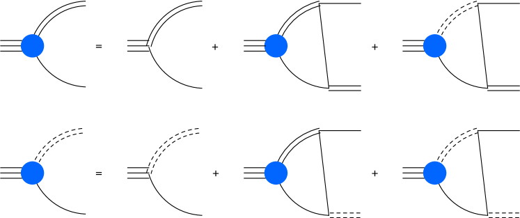
Figure 1: Diagrammatic representation of the LO three-body CP-even vertex function. The (dashed) double line denotes a dressed spin-singlet (spin-triplet) dibaryon propagator.

The LO vertex function $\bm{\mathcal{G}}(E,p)$ [[for a three-nucleon system in the center-of-mass frame with binding energy $E$ and relative momentum ${\bf p}$ between outgoing nucleon and dimer]] is given by the integral equation shown diagrammatically in Fig. 1 and given explicitly by

$$\bm{\mathcal{G}}(E,p)=\widetilde{\mathbf{1}}+\mathbf{K}^{0}(q,p,E)\otimes_{q}\bm{\mathcal{\widetilde{G}}}(E,q)~{}.$$ (10)

We define the short-hand notation

$$\bm{\mathcal{\widetilde{G}}}(E,q)=\bm{D}\left(E-\frac{q^{2}}{2M_{N}},q\right)\bm{\mathcal{G}}(E,q)$$ (11)

where

$$\bm{D}\left(E-\frac{q^{2}}{2M_{N}},q\right)=\left(\begin{matrix}D_{t}\left(E-\frac{q^{2}}{2M_{N}},q\right)&0\\ 0&D_{s}\left(E-\frac{q^{2}}{2M_{N}},q\right)\end{matrix}\right),$$ (12)

and the inhomogeneous term in this integral equation is

$$\widetilde{\mathbf{1}}=\left(\begin{array}[]{rr}1\\ -1\end{array}\right)~{}.$$ (13)

The convolution operator $\otimes_{q}$ is defined as

$$A(q)\otimes_{q}B(q)=\int_{0}^{\Lambda}dq\frac{q^{2}}{2\pi^{2}}A(q)B(q)~{},$$ (14)

where $\Lambda$ is a hard momentum-space cutoff. Observables will be $\Lambda$-independent for large cutoffs.

The homogeneous term is defined by

$$\mathbf{K}^{\ell}(q,p,E)=R_{\ell}(q,p,E)\left(\begin{array}[]{rr}-1&3\\ 3&-1\end{array}\right)~{},$$ (15)

where the function $R_{\ell}$ is defined as

$$R_{\ell}(q,p,E) =\frac{2\pi}{qp}Q_{\ell}\left(\frac{q^{2}+p^{2}-M_{N}E-i\epsilon}{qp}\right)~{},$$ (16)

and $Q_{l}$ are functions proportionial to Legendre function of the second kind but differ from their conventional definition by a phase of $(-1)^{\ell}$,

$$Q_{\ell}(a)=\frac{1}{2}\int_{-1}^{1}\frac{P_{\ell}(x)}{a+x}\hbox{d}x~{}.$$ (17)

III The T-odd vertex function

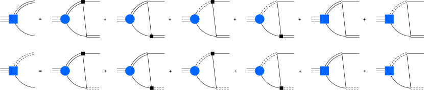
Figure 2: $\not{P}\not{T}$ vertex function. A blue square denotes the $\not{P}\not{T}$ vertex function, while a black square an insertion of the operators in Eq. (8). Remaining notation as in Fig. 1.

A three-particle irreducible diagram can contain repeated nucleon-dimer scattering between a nucleon-photon vertex and an insertion of a two-nucleon CP-odd vertex. We include these diagrams through two integral equations that generate a vertex function that contains a single insertion of the CP-odd two-nucleon interaction. The diagrammatic expression for these vertex functions is shown in Fig. 2.

The T-odd vertices convert the spin $1/2$, isospin $1/2$ trimer field $\psi$ into a nucleon-dimer with three possible spin/isospin quantum numbers: spin and isospin $1/2$, spin $1/2$ and isospin $3/2$, as well as spin $3/2$ and isospin $1/2$. The latter does not contribute to the three-nucleon EDM at leading order, since the LO electromagnetic interaction does not change spin and the overlap of the spin 3/2 T-odd function with the triton or helion vanishes. The integral equations for the isospin 1/2 component, $\bm{\mathcal{T}}^{\frac{1}{2}}$, and the isospin 3/2 component, $\bm{\mathcal{T}}^{\frac{3}{2}}$, of the spin-1/2 T-odd vertex functions are given by

$$(\boldsymbol{\sigma}\cdot{\bf k})\bm{\mathcal{T}}^{\frac{1}{2}}(E,k)=(\boldsymbol{\sigma}\cdot{\bf k})\left\{\bm{R}^{\frac{1}{2}}_{\mathcal{T}}(E,k,q)\otimes_{q}\widetilde{\bm{\mathcal{T}}}^{\frac{1}{2}}(E,q)+\bm{R}^{\frac{1}{2}}(E,k,q)\otimes_{q}\bm{\widetilde{\mathcal{G}}}(E,q)\right\}~{},$$ (18)

$$(\boldsymbol{\sigma}\cdot{\bf k})(\delta^{3c}+\tau^{3}\tau^{c})\bm{\mathcal{T}}^{\frac{3}{2}}(E,k)=(\boldsymbol{\sigma}\cdot{\bf k})(\delta^{3c}+\tau^{3}\tau^{c})\Big{\{}\bm{R}^{\frac{3}{2}}_{\mathcal{T}}(E,k,q)\otimes_{q}\widetilde{\bm{\mathcal{T}}}^{\frac{3}{2}}(E,q)$$

$$\qquad\qquad\qquad\qquad\qquad\qquad\qquad+\bm{R}^{\frac{3}{2}}(E,k,q)\otimes_{q}\bm{\widetilde{\mathcal{G}}}(E,q)\Big{\}}~{},$$ (19)

where we show explicitly the spin/isospin structure of the vertex functions, and, similarly to the CP-even case, we introduced the shorthand notation for the product of a vertex function and a dressed dibaryon propagator

$$\widetilde{\bm{\mathcal{T}}}^{\frac{1}{2},\frac{3}{2}}(E,q)=\bm{D}\left(E-\frac{q^{2}}{2M_{N}},q\right)\bm{\mathcal{T}}^{\frac{1}{2},\frac{3}{2}}(E,q)~{}.$$ (20)

The kernels of the homogeneous terms are

$$\bm{R}^{\frac{1}{2}}_{\mathcal{T}}(E,k,q) =\frac{q}{k}R_{1}(E,k,q)\begin{pmatrix}-1&\phantom{-}3\\ \phantom{-}3&-1\end{pmatrix},\qquad\bm{R}^{\frac{3}{2}}_{\mathcal{T}}(E,k,q)=\frac{q}{k}R_{1}(E,k,q)\left(\begin{matrix}0&0\\ 0&2\end{matrix}\right).$$ (21)

The inhomogeneous terms are driven by the T-odd operators in Eq. (8). The isospin 1/2 vertex functions receive contributions from both isoscalar and isovector operators in Eq. (8),

$$\bm{R}^{\frac{1}{2}}(E,k,q) =\left[R_{0}(E,k,q)\begin{pmatrix}-1&1\\ -2&0\end{pmatrix}+\frac{q}{k}R_{1}(E,k,q)\left(\begin{matrix}\phantom{-}1&2\\ -1&0\end{matrix}\right)\right]\left(C_{{}^{3}S_{1}-^{1}P_{1}}+\frac{2}{3}\tau^{3}C_{{}^{3}S_{1}-^{3}P_{1}}\right)$$

$$+\left[R_{0}(E,k,q)\left(\begin{matrix}\phantom{+}0&2\\ -1&1\end{matrix}\right)-\frac{q}{k}R_{1}(E,k,q)\left(\begin{matrix}0&-1\\ 2&\phantom{+}1\end{matrix}\right)\right]\left(C^{(0)}_{{}^{1}S_{0}-^{3}P_{0}}-\frac{2}{3}\tau^{3}C^{(1)}_{{}^{1}S_{0}-^{3}P_{0}}\right).$$ (22)

The isospin $3/2$ component is induced by the isotensor operator $C^{(2)}_{{}^{1}S_{0}-^{3}P_{0}}$ and by the isovector operators yielding

$$\bm{R}^{\frac{3}{2}}(E,k,q) = \left[2R_{0}(E,k,q)+\frac{q}{k}R_{1}(E,k,q)\right]\left(\begin{matrix}0&0\\ 1&0\end{matrix}\right)\frac{4}{3}C_{{}^{3}S_{1}-^{3}P_{1}}$$

$$-\frac{1}{3}\left[R_{0}(E,k,q)\left(\begin{matrix}0&0\\ 1&5\end{matrix}\right)+\frac{q}{k}R_{1}(E,k,q)\left(\begin{matrix}0&0\\ 2&4\end{matrix}\right)\right]\left(C^{(1)}_{{}^{1}S_{0}-^{3}P_{0}}-3\tau_{3}C^{(2)}_{{}^{1}S_{0}-^{3}P_{0}}\right).$$

III.1 Integral equations in the SU(4) limit

Nuclear interactions exhibit an approximate $SU(4)$ spin-isospin (Wigner) symmetry, which would be exact in the limit Wigner (1937); Vanasse and Phillips (2017) of equal spin-triplet and singlet scattering lengths. $SU(4)$ breaking is parameterized by the difference $\gamma_{t}-\gamma_{s}$, and the expansion around the Wigner limit converges very well Vanasse and Phillips (2017). We will study the electric dipole form factor of the three-nucleon system in the $SU(4)$ limit, and provide the relevant formulae in this section.

In the $SU(4)$ limit, $D_{t}=D_{s}=D_{SU(4)}$ and from Eq. (10) one can see that $\widetilde{\mathcal{G}}_{t}=-\widetilde{\mathcal{G}}_{s}$. We can introduce the combinations

$${\mathcal{G}}_{\pm}=\frac{1}{2}\left({\mathcal{G}}_{t}\mp{\mathcal{G}}_{s}\right),$$ (24)

so that $\widetilde{\mathcal{G}}_{-}$ vanishes in the $SU(4)$ limit.

The structure of the T-odd vertex functions simplifies significantly in the $SU(4)$ limit. It can be shown that both the isospin 1/2 and isospin 3/2 components are proportional to a single function $\mathcal{T}_{SU(4)}$, which satisfies the integral equation

$$\mathcal{T}_{SU(4)}(E,k) =-\mathcal{R}_{SU(4)}(E,k,q)\otimes_{q}\widetilde{\mathcal{G}}_{+}(E,q)+2\frac{q}{k}R_{1}(E,k,q)\otimes_{q}\widetilde{\mathcal{T}}_{SU(4)}(E,q)~{},$$ (25)

$$\mathcal{R}_{SU(4)}(E,k,q) =2R_{0}(E,k,q)+\frac{q}{k}R_{1}(E,k,q).$$ (26)

In terms of $\mathcal{T}_{SU(4)}$, we can write

$$\bm{\mathcal{T}}_{SU(4)}^{\frac{1}{2}}(E,k)=\left(\begin{matrix}1\\ 1\end{matrix}\right)\mathcal{T}_{SU(4)}^{\frac{1}{2}}(E,k)~{},\quad\bm{\mathcal{T}}_{SU(4)}^{\frac{3}{2}}(E,k)=\left(\begin{matrix}0\\ 1\end{matrix}\right)\mathcal{T}_{SU(4)}^{\frac{3}{2}}(E,k)~{},$$ (27)

where

$$\mathcal{T}_{SU(4)}^{\frac{1}{2}}(E,k) =\bigg{[}C^{(0)}_{{}^{1}S_{0}-^{3}P_{0}}+C_{{}^{3}S_{1}-^{1}P_{1}}+\frac{2\tau^{3}}{3}(C_{{}^{3}S_{1}-^{3}P_{1}}-C^{(1)}_{{}^{1}S_{0}-^{3}P_{0}})\bigg{]}\mathcal{T}_{SU(4)}(E,k)~{},$$ (28)

$$\mathcal{T}_{SU(4)}^{\frac{3}{2}}(E,k) =\bigg{[}-\frac{2}{3}(2C_{{}^{3}S_{1}-^{3}P_{1}}+C^{(1)}_{{}^{1}S_{0}-^{3}P_{0}})+2\tau^{3}C^{(2)}_{{}^{1}S_{0}-^{3}P_{0}}\bigg{]}\mathcal{T}_{SU(4)}(E,k)~{}.$$ (29)

IV Three-nucleon form factors

The EDFF of a three-nucleon system can be obtained from the matrix element of the zero-component of the electromagnetic current $J^{0}$ in the presence of CP violation. Neglecting recoil corrections, we can write the matrix element of $J^{0}$ as

$$\langle{\bf p}^{\prime},\alpha|J^{0}|{\bf p},\beta\rangle=F_{C}(q^{2})\delta_{\alpha\beta}+\left[\boldsymbol{\sigma}\cdot{\bf q}\right]_{\alpha\beta}F_{D}(q^{2}),$$ (30)

where $\alpha$ and $\beta$ are spin indices of the in- and outgoing three-nucleon state, ${\bf q}={\bf p}-{\bf p}^{\prime}$ is the momentum injected by the current, and $q=|\textbf{q}|$. $F_{C}$ denotes the charge form factor and $F_{D}$ the electric dipole form factor, which vanishes in the absence of CP-violation. We will write the EDFF in terms of two components,

$$F_{D}(q^{2})=F_{\rm I}(q^{2})+F_{\rm II}(q^{2}).$$ (31)

$F_{\rm I}$ denotes the EDFF generated by the T-odd component of the electromagnetic current, which is dominated by one-nucleon operators, namely the neutron and proton EDMs in Eqs. (6). CPV interactions can in addition generate a CP-odd component in the three-nucleon wavefunction, which is dominated by the two-body operators in Eq. (8). We denote the ensuing EDFF by $F_{\rm II}$.

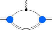
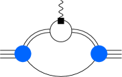
Figure 3: Diagrams contributing to the one-body component of the EDFF, defined in Eq. (32). Here, the double line can denote a spin-triplet or singlet dimer. The black square denotes an insertion of the nucleon EDM, defined in Eq. (6).

The diagrams contributing to $F_{I}$ are shown in Fig. 3, where the black square denotes an insertion of the nucleon EDM, defined in Eq. (6). We therefore write the $F_{\rm I}$ as the sum of the three terms

$$F_{\rm I}(q^{2})=F_{\rm I}^{A}(q^{2})+F_{\rm I}^{B}(q^{2})+F_{\rm I}^{C}(q^{2})~{},$$ (32)

corresponding to the three diagrams shown in Fig. 3. We give explicit expressions for the diagrams in Appendix B. From the expression in Appendix B and the charge form factor in Refs. Vanasse (2017, 2018), which we also report in Appendix B, it can be seen that in the $SU(4)$ limit, the one-body contribution to the triton and ³He EDFFs is identical to $F_{C}(q^{2})$, weighted by the proton or neutron EDM,

$$F_{\rm I}(q^{2},^{3}{\rm H})\xrightarrow{SU(4)}d_{p}\,F_{C}(q^{2}),\qquad F_{\rm I}(q^{2},^{3}{\rm He})\xrightarrow{SU(4)}d_{n}F_{C}(q^{2}).$$ (33)

We will see that the results at the physical values of $\gamma_{s}$ and $\gamma_{t}$ deviate from this expectation by a few percent.

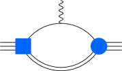
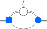
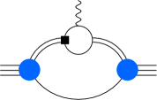
Figure 4: Diagrams for the three-nucleon EDM form factor at LO that involve a CP-odd two-nucleon interaction.

The second class of contributions arises from the two-nucleon operators given in Eq. (8). In Fig. 4 we show the EDFF topologies that include a CP-odd two-nucleon operator. Diagrams $(a)$, $(b)$ and $(c)$ include the T-odd vertex functions defined in Section III. Diagram $(d)$ and $(e)$ include the CP-even $\mathcal{G}$ vertex functions, with an additional insertion of the T-odd nucleon-dimer operators. For simplicity, we only show one topology. The complete set of diagrams also includes the insertions of the T-odd operators to the left of the photon-nucleon vertex.

We write the sum of contributions to the EDFF that include two-body CP-odd interactions as

$$F_{\rm II}(q^{2})=F_{\rm II}^{A}(q^{2})+F_{\rm II}^{B}(q^{2})+F_{\rm II}^{C}(q^{2})+F_{\rm II}^{D}(q^{2})+F_{\rm II}^{E}(q^{2})~{},$$ (34)

where the superscript indicates the corresponding diagram in Fig.4. We give explicit expressions for the individual diagrams in Appendix C.

In the $SU(4)$ limit, the two-body diagrams also undergo a noticeable simplification, and they become proportional to a single combination of T-odd coefficients,

$$F_{\rm II}(q^{2},^{3}{\rm H}) \xrightarrow{SU(4)} \tilde{F}_{SU(4)}(q^{2})\left(C_{{}^{3}S_{1}-^{1}P_{1}}+C^{(0)}_{{}^{1}S_{0}-3P_{0}}-2C^{(2)}_{{}^{1}S_{0}-^{3}P_{0}}-2C_{{}^{3}S_{1}-^{3}P_{1}}\right),$$ (35)

$$F_{\rm II}(q^{2},^{3}{\rm He}) \xrightarrow{SU(4)} -\tilde{F}_{SU(4)}(q^{2})\left(C_{{}^{3}S_{1}-^{1}P_{1}}+C^{(0)}_{{}^{1}S_{0}-3P_{0}}-2C^{(2)}_{{}^{1}S_{0}-^{3}P_{0}}+2C_{{}^{3}S_{1}-^{3}P_{1}}\right)~{},$$ (36)

where $\tilde{F}_{SU(4)}(q^{2})$ is a universal function that depends on $q$, on the scattering length in the Wigner limit and the three-body binding energy. In particular, the three-nucleon EDM becomes insensitive to the isospin-1 $C^{(1)}_{{}^{1}S_{0}-^{3}P_{0}}$ operator.

V Results

We have calculated the numerical coefficients multiplying the low-energy constants that appear in a decomposition of the CP-odd form factor as a function of $q^{2}$. In the absence of the Coulomb interaction, we take the binding energy of ³H and ³He to be equal, i.e. $B(^{3}{\rm H})=B(^{3}{\rm He})$. We estimate the numerical uncertainty of the results presented below to be 1 % or lower. The theoretical uncertainty of our results is determined by the expansion parameter of the pionless EFT which is $\gamma_{t}\rho_{t}\approx 0.4$, where $\rho_{t}$ is the effective range in the triplet channel. The theoretical uncertainties of our results are therefore clearly larger than the numerical ones.

The EDFF results obtained for ³H are shown in Fig. 5. In Table 1 we show the cutoff dependence of the dipole moment contributions arising from the different EFT operators. Furthermore, we observe that cutoffs larger than $~{}1.5$ GeV are needed to obtain numerically converged results. This convergence behavior is shown for the EDMs in Fig. 6.

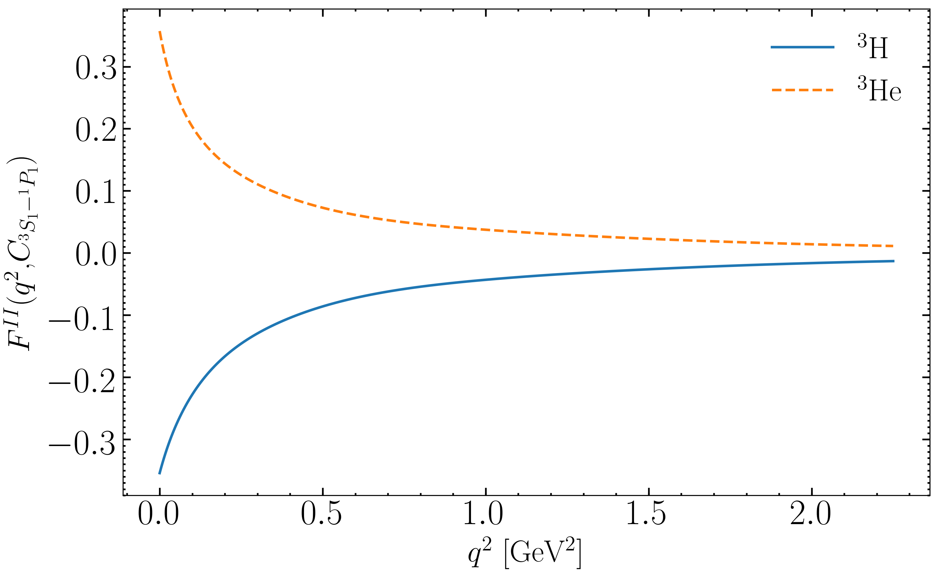
(a) $C_{{}^{3}S_{1}-^{1}P_{1}}$

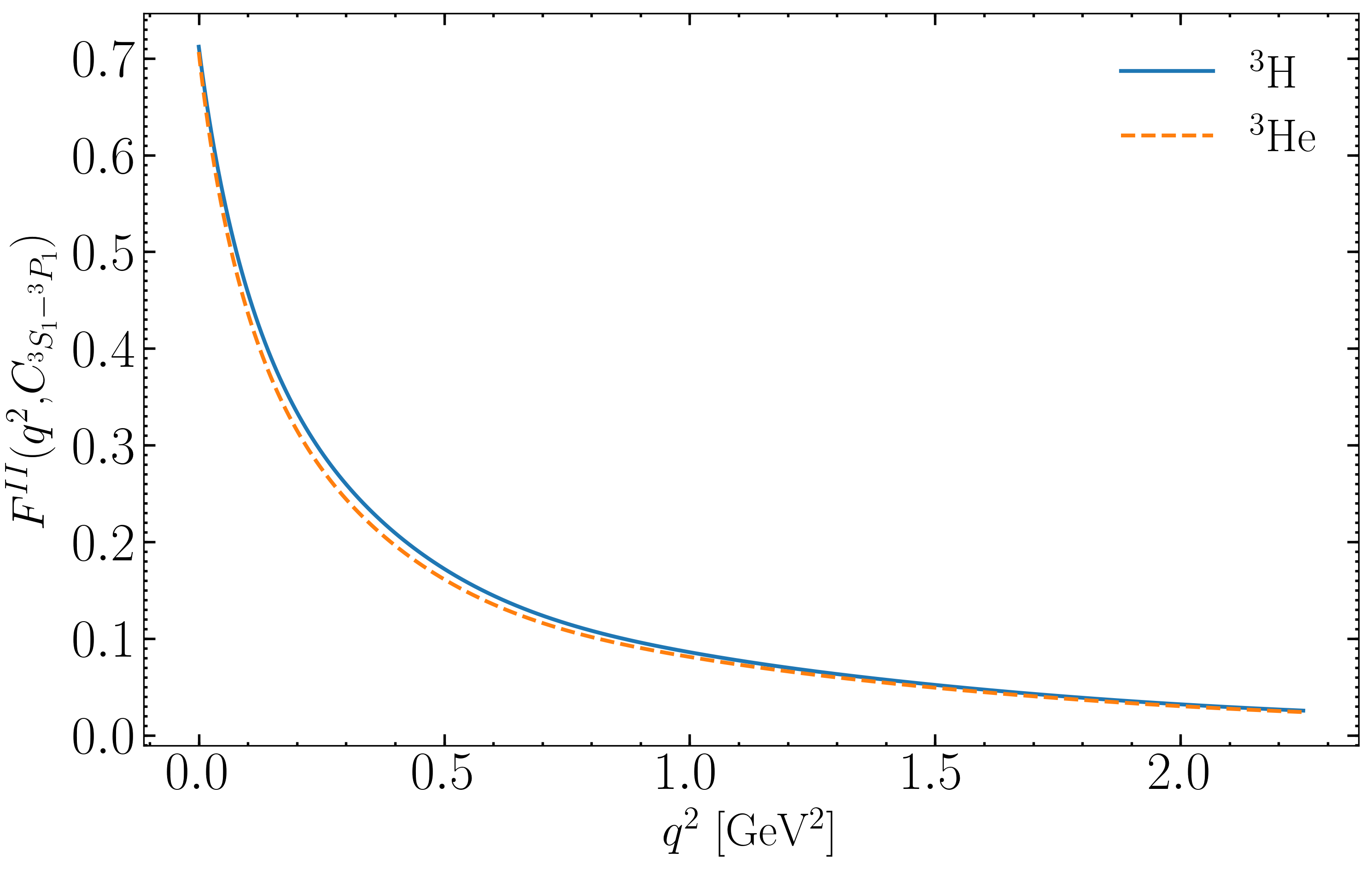
(b) $C_{{}^{3}S_{1}-^{3}P_{1}}$

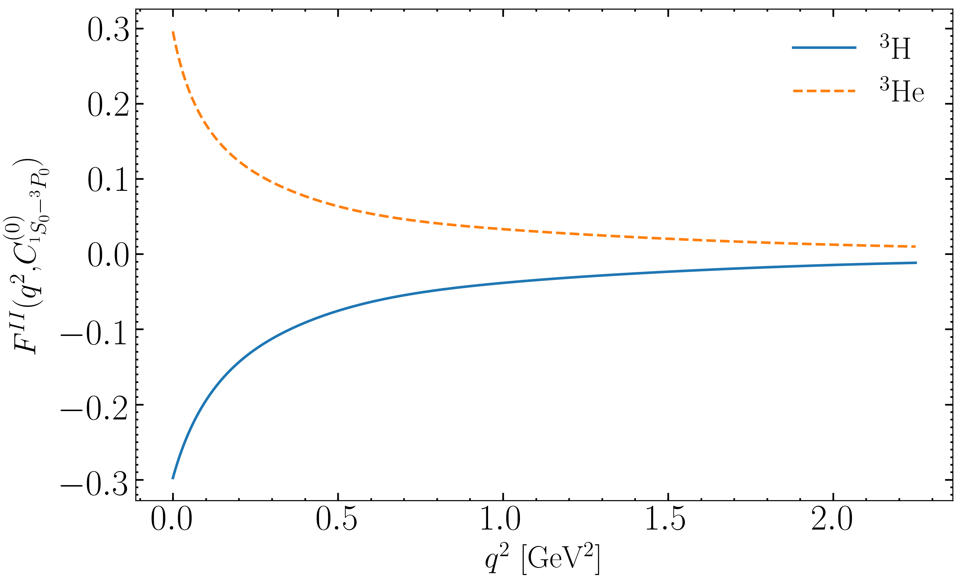
(c) $C_{{}^{1}S_{0}-^{3}P_{0}}^{(0)}$

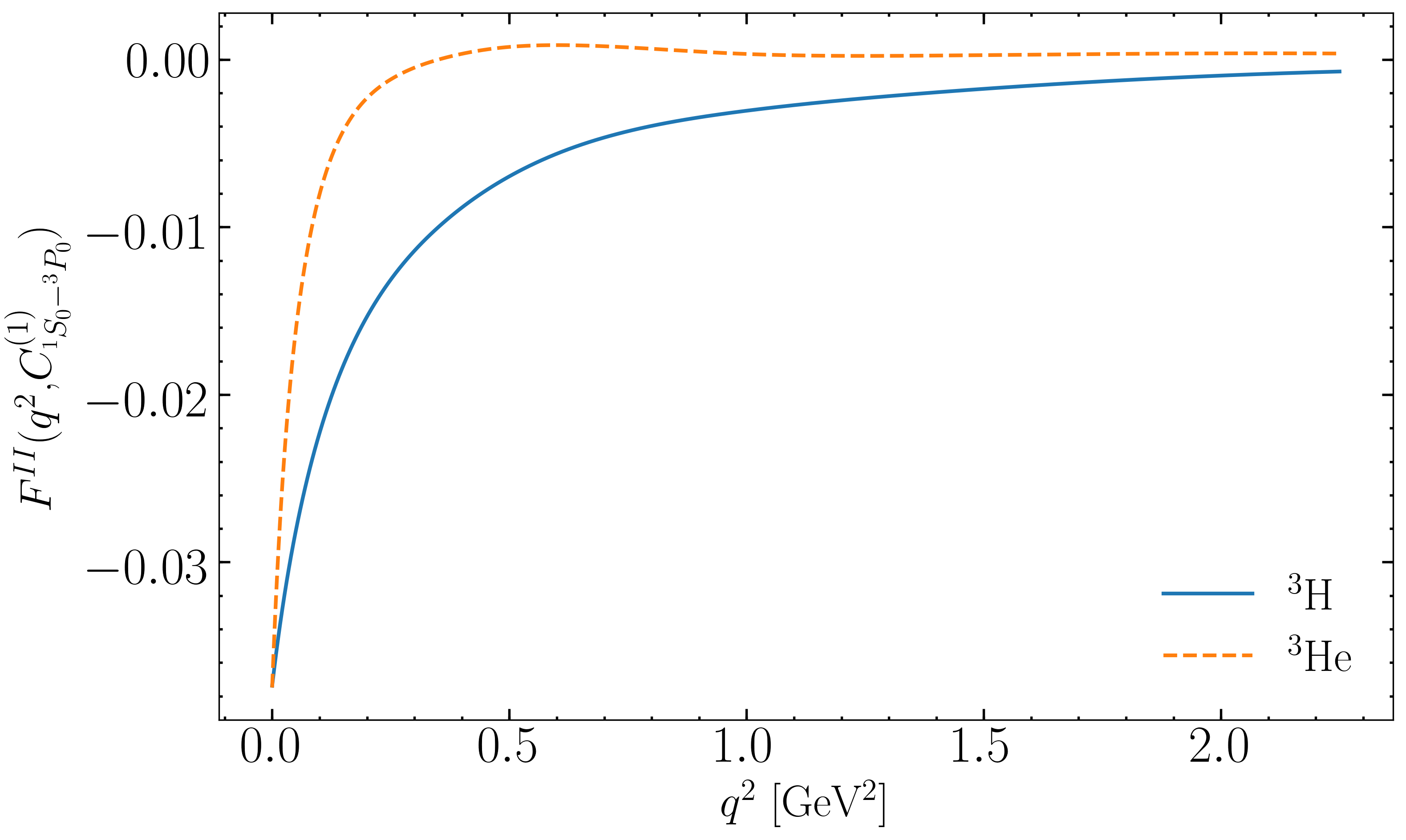
(d) $C_{{}^{1}S_{0}-^{3}P_{0}}^{(1)}$

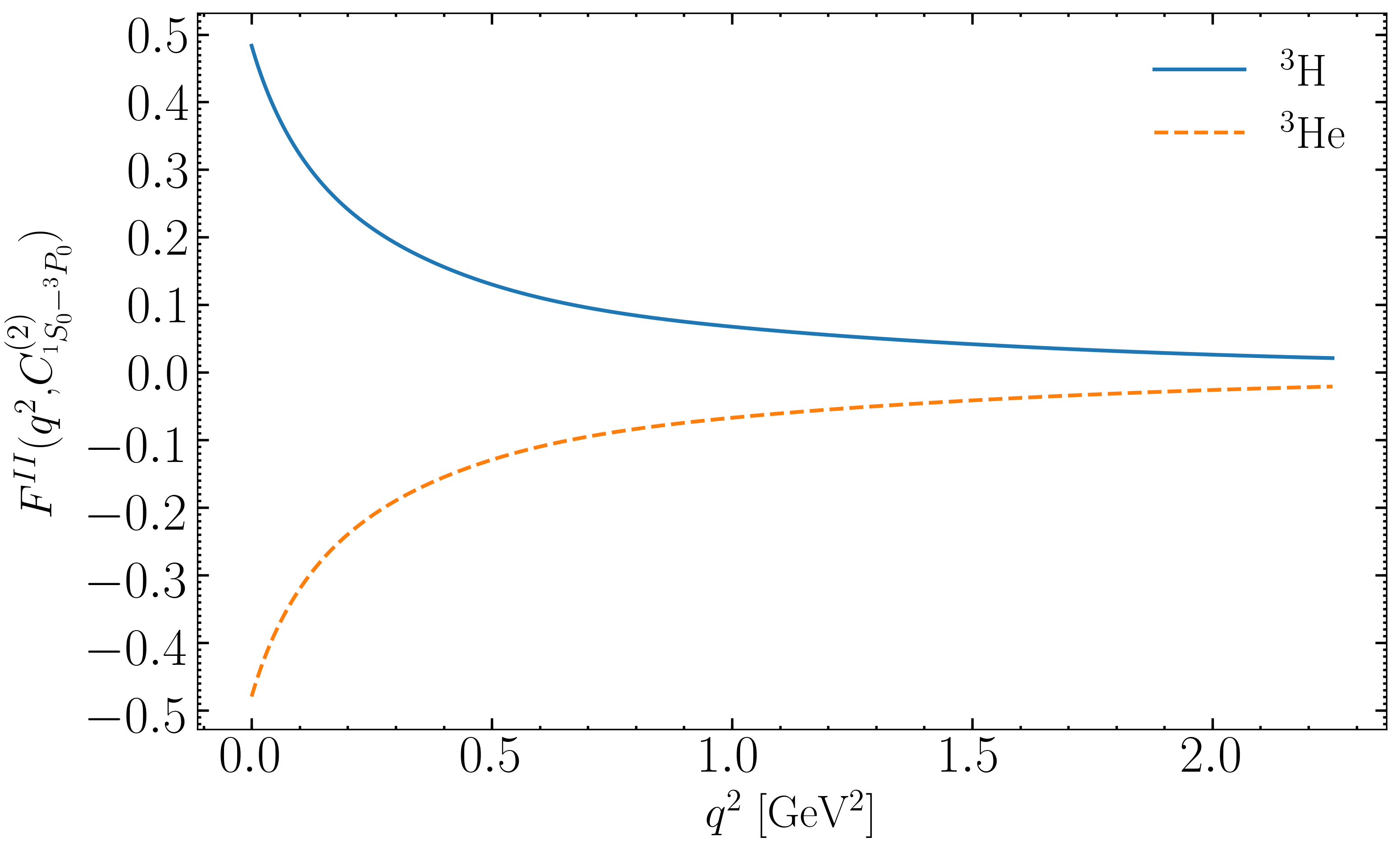
(e) $C_{{}^{1}S_{0}-^{3}P_{0}}^{(2)}$

Figure 5: The EDFF contributions arising from five different two-nucleon CP-odd operators as a function of $q^{2}$.

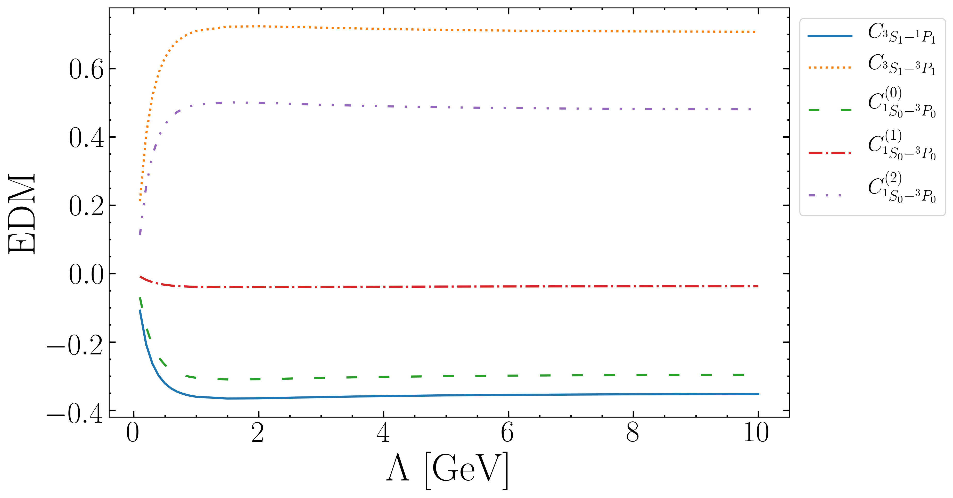
Figure 6: Cutoff dependence of the ³H EDM two-nucleon contributions.

At small $q^{2}$, we will expand the charge form factor as

$$F_{C}(q^{2}) = Z\left(1-\frac{q^{2}}{6}\langle r^{2}_{c}\rangle+\frac{1}{5!}\langle r^{4}_{c}\rangle q^{4}+\ldots\right)~{},$$ (37)

where $r^{2}_{c}$ is the charge squared radius and $r^{4}_{c}$ the 4^th Zeemach moment, $Z$ denotes the total charge of the nucleus considered and we omitted a label to denote the specific nucleus. We define a similar expansion for the one- and two-body EDFF,

$$F_{i}(q^{2},C) = d_{i}(C)\left(1-\frac{q^{2}}{6}\langle r^{2}_{d,\,i}(C)\rangle+\frac{1}{5!}\langle r^{4}_{d,\,i}(C)\rangle q^{4}+\ldots\right),$$ (38)

where $i=\rm{I},\rm{II}$. $C=d_{n,p}$ for the one-body term, while it denotes one of the nucleon-dimer T-odd operators in Eq. (8) for the two-body contribution. In the $SU(4)$ limit, all the dependence on couplings factorizes into the universal function $\tilde{F}_{SU(4)}(q^{2})$ and a linear combination of low-energy constants, as shown in Eqs. (35) and (90). The square radius of the EDFF is particularly important since it determines the nuclear Schiff moment, and thus the EDMs of the atomic ³H and ³He species Schiff (1963). More precisely, the Schiff moment is proportional to the difference of the charge and dipole radii de Jesus and Engel (2005)

$$S_{i}(C)=-\frac{d_{i}(C)}{6}\left(\langle r^{2}_{d,\,i}(C)\rangle-\langle r^{2}_{c}\rangle\right)~{},$$ (39)

where again $i$ denotes either the one- (I) or two-body (II) contribution.

The three-nucleon charge form factor in EFT($\not{\pi}$) has already been computed in Refs. Platter and Hammer (2006); Vanasse (2017, 2018), including next-to-leading order (NLO) and next-to-next-to-leading order (N²LO) corrections. At LO, and neglecting Coulomb interactions, one finds

$$\langle r^{2}_{c}(^{3}{\rm H})\rangle=1.28\,{\rm fm}^{2}~{},\qquad\langle r^{2}_{c}(^{3}{\rm He})\rangle=1.56\,{\rm fm}^{2}~{}.$$ (40)

These results are in agreement with those in Refs. Vanasse (2017, 2018). We will use the charge form factor as a point of comparison for the momentum dependence of the EDFF. In the $SU(4)$ limit,

$$\langle r^{2}_{c}(^{3}{\rm H})\rangle =\langle r^{2}_{c}(^{3}{\rm He})\rangle=1.32\,{\rm fm}^{2}.$$ (41)

$\Lambda$ (GeV)	$d_{p}$	$d_{n}$	$C_{{}^{3}S_{1}-^{1}P_{1}}$	$C_{{}^{3}S_{1}-^{3}P_{1}}$	$C_{{}^{1}S_{0}-^{3}P_{0}}^{(0)}$	$C_{{}^{1}S_{0}-^{3}P_{0}}^{(1)}$	$C_{{}^{1}S_{0}-^{3}P_{0}}^{(2)}$
10	0.982	0.008	-0.358	0.708	-0.297	-0.038	0.481
30	0.988	0.010	-0.356	0.706	-0.295	-0.037	0.479
80	0.990	0.010	-0.358	0.708	-0.297	-0.038	0.481
600	0.991	0.010	-0.359	0.708	-0.298	-0.038	0.481

Table 1: Coefficients of the ³H EDM low-energy constants for different values of the cutoff $\Lambda$.

The neutron and proton EDMs contributions to the ³H and ³He EDM are given by

$$d_{\rm I}(^{3}{\rm H}) = 0.99\,d_{p}+9.7\cdot 10^{-3}d_{n},\qquad d_{\rm I}(^{3}{\rm He})=0.99\,d_{n}+9.7\cdot 10^{-3}d_{p}.$$ (42)

The EDM only deviates by 1% from the expectation in the Wigner limit. These results can be compared with chiral EFT calculations of Ref. de Vries et al. (2011a); Bsaisou et al. (2015a); Gnech and Viviani (2020). These calculations include subleading effects in the strong potential, and thus in the three-nucleon wavefunctions, and typically find the $d_{p}$ ($d_{n}$) contribution to ³H (³He) EDM to be roughly 10% smaller than Eq. (42).

The dominant momentum dependence of the EDFF is encoded by the dipole square radius, which we find to be

$$\langle r^{2}_{d,\,{\rm I}}(^{3}{\rm H},d_{n})\rangle = -18.3\,{\rm fm}^{2},\qquad\langle r^{2}_{d,\,{\rm I}}(^{3}{\rm H},d_{p})\rangle=1.28\,{\rm fm}^{2},$$ (43)

$$\langle r^{2}_{d,\,{\rm I}}(^{3}{\rm He},d_{n})\rangle = 1.28\,{\rm fm}^{2},\qquad\langle r^{2}_{d,\,{\rm I}}(^{3}{\rm He},d_{p})\rangle=-18.3\,{\rm fm}^{2}.$$ (44)

The square radii agree very well with the triton charge radius. This has consequences for the Schiff moment, and thus the EDMs of atomic ³He and ³H. We see that in the case of ³H, the one-body Schiff moment vanishes at LO in EFT($\not{\pi}$), $S_{\rm I}(^{3}{\rm H},d_{p})=0$. The one-body Schiff moment of ³He is small, but non-vanishing,

$$S_{\rm I}(^{3}{\rm He},d_{n})=\frac{d_{n}}{6}\left(0.28\right)\,{\rm fm}^{2}.$$ (45)

We adopt the same expansion as Eq. (38) for the function $F_{SU(4)}(q^{2})$ and obtain for the two-body form factor in the $SU(4)$ limit

$$d_{SU(4)}=-0.332,\qquad\langle r^{2}_{d}\rangle_{SU(4)}=1.32\,\textrm{fm}^{2}.$$ (46)

where we used the average of spin-singlet and triplet binding momentum and the triton binding energy in our calculation. In this limit, the momentum dependence of the form factor seems to be dictated by the charge form factor, and we find that, to very good approximation,

$$\frac{\tilde{F}_{SU(4)}(q^{2})}{F_{C}(q^{2})}={\rm constant}.$$ (47)

For $q$ between 0 and 500 MeV, this ratio deviates from a constant at the per mille level. At the physical value of the scattering lengths, the ³H and ³He EDMs from the two-body form factor $F_{\rm II}$ are given by

$$d_{\rm II}(^{3}{\rm H}) = -0.358C_{{}^{3}S_{1}-^{1}P_{1}}+0.707C_{{}^{3}S_{1}-^{3}P_{1}}-0.297C^{(0)}_{{}^{1}S_{0}-^{3}P_{0}}$$ (48)

$$-0.0368C^{(1)}_{{}^{1}S_{0}-^{3}P_{0}}+0.480C^{(2)}_{{}^{1}S_{0}-^{3}P_{0}},$$

$$d_{\rm II}(^{3}{\rm He}) = 0.358C_{{}^{3}S_{1}-^{1}P_{1}}+0.707C_{{}^{3}S_{1}-^{3}P_{1}}+0.297C^{(0)}_{{}^{1}S_{0}-^{3}P_{0}}$$ (49)

$$-0.0375C^{(1)}_{{}^{1}S_{0}-^{3}P_{0}}-0.480C^{(2)}_{{}^{1}S_{0}-^{3}P_{0}}.$$

where, as our central value, we took the EDFF at $\Lambda=60$ GeV. As already remarked, the numerical accuracy is a the percent level, and smaller than the LO EFT($\not{\pi}$) theoretical uncertainty. The EDFF square radii induced by the CPV operators in Eq. (8) are given in Table 2.

We notice that, in the absence of the Coulomb interaction, the EDMs of ³H and ³He follow simple isospin relations. In particular, the isoscalar and isotensor operators give rise to an isovector EDM, while the isovector operators to an isoscalar three-nucleon EDM. These patterns can be understood by noticing that only the isovector piece of the CP-even one-body electromagnetic current $J^{0}$ contributes to $F_{\rm II}$ Liu and Timmermans (2004); Stetcu et al. (2008); de Vries et al. (2011a).

		$C_{{}^{3}S_{1}-^{1}P_{1}}$	$C_{{}^{3}S_{1}-^{3}P_{1}}$	$C_{{}^{1}S_{0}-^{3}P_{0}}^{(0)}$	$C_{{}^{1}S_{0}-^{3}P_{0}}^{(1)}$	$C_{{}^{1}S_{0}-^{3}P_{0}}^{(2)}$
$\langle r^{2}_{d,\,{\rm II}}(^{3}{\rm H})\rangle$	(fm2)	1.31	1.30	1.24	1.48	1.19
$\langle r^{2}_{d,\,{\rm II}}(^{3}{\rm He})\rangle$	(fm2)	1.90	1.50	1.83	4.58	1.19

Table 2: Square radii of the two-body EDFF induced by the CPV operators in Eq. (8), computed at $\Lambda=60$ GeV. The $C_{{}^{1}S_{0}-^{3}P_{0}}^{(1)}$ squared radii have a numerical error of approximately 10 % since the corresponding dipole moments are relatively small. The other radii have few-percent numerical uncertainties, which we do not show.

We observe that the EDM induced by the isoscalar operators $C_{{}^{3}S_{1}-^{1}P_{1}}$ and $C^{(0)}_{{}^{1}S_{0}-^{3}P_{0}}$ and by the isospin-1 operator $C_{{}^{3}S_{1}-^{3}P_{1}}$ deviate from the $SU(4)$ limit by about 10%. The EDM from the operators that connect the ${}^{3}S_{1}$ to ${}^{1}P_{1}$ and ${}^{3}P_{1}$ waves increases (in absolute value) by 10%, while the EDM from $C^{(0)}_{{}^{1}S_{0}-^{3}P_{0}}$ decreases by the same amount. We also note that the isotensor operator $C^{(2)}_{{}^{1}S_{0}-^{3}P_{0}}$ shows a larger, 30% variation, from the Wigner limit. Furthermore, we find that, with the exception of $C^{(1)}_{{}^{1}S_{0}-^{3}P_{0}}$, all operators induce matrix elements of $\mathcal{O}(1)$, as naively expected. The contribution of $C^{(1)}_{{}^{1}S_{0}-^{3}P_{0}}$ is suppressed by roughly a factor of ten. It is interesting to note that in the case of ³H, the momentum dependence of the form factor induced by $C_{{}^{3}S_{1}-^{1}P_{1}}$, $C_{{}^{3}S_{1}-^{3}P_{1}}$ and $C^{(0)}_{{}^{1}S_{0}-^{3}P_{0}}$ cannot be distinguished from the charged form factor within error. This leads to $S_{\rm II}$ being compatible with zero, implying that for these operators the Schiff moment vanishes at LO in pionless EFT. $C^{(2)}_{{}^{1}S_{0}-^{3}P_{0}}$ induces a non-zero, but small Schiff moment. Specifically, in the case of ³He, all operators induce a non-zero Schiff moment, but also in this case we expect subleading corrections in EFT($\not{\pi}$) to be important.

VI Summary

In this work, we have shown that EFT($\not{\pi}$) is an efficient framework that facilitates a straightforward calculation of the EDMs and their corresponding form factors of three-nucleon systems. We focused on the ³H and ³He systems at leading order in the pionless EFT expansion and neglected Coulomb effects in the ³He system. At this order, the only (CP-even) parameters that enter our calculation are the deuteron binding energy, the two-nucleon spin-singlet scattering length, and the three-body binding energy of the state under consideration. Allowing for CP-odd interactions in the few-nucleon sectors leads to a total of 7 parameters, where two of them are the neutron and proton EDM and 5 arise from short-distance physics in the two-nucleon system.

The deuteron and the isoscalar combination of the ³H and ³He EDMs are mostly sensitive to the isovector coupling $C_{{}^{3}S_{1}-^{3}P_{1}}$ (see App. A for a derivation of the EDFF and resulting EDM in pionless EFT). These two observables are thus largely degenerate, and, neglecting the one-body piece, our calculation finds

$$\frac{d(^{3}{\rm H})+d(^{3}{\rm He})}{2d(^{2}{\rm H})}=0.71.$$ (50)

For comparison, the chiral EFT calculation of Ref. Gnech and Viviani (2020) finds the ratio to be between $0.77$ and $0.80$, for both the isovector pion-nucleon coupling $\bar{g}_{1}$ and for the linear combination $A_{3}-A_{4}$, which corresponds to $C_{{}^{3}S_{1}-^{3}P_{1}}$. The isovector combination $d(^{3}{\rm H})-d(^{3}{\rm He})$ probes the isoscalar couplings $C_{{}^{3}S_{1}-^{1}P_{1}}$, $C^{(0)}_{{}^{1}S_{0}-^{3}P_{0}}$ and the isotensor $C^{(2)}_{{}^{1}S_{0}-^{3}P_{0}}$, which are particularly important for the QCD $\bar{\theta}$ term. In chiral EFT, this linear combination cannot be expressed only in terms of pion-nucleon CPV couplings, but requires short-range nucleon-nucleon operators at LO de Vries et al. (2020b).

Specializing to the QCD $\bar{\theta}$-term, we combine Eqs. (42) and (49) to obtain

$$d_{{}^{3}{\rm He}}(\bar{\theta}) = d_{n}+0.358~{}C_{{}^{3}S_{1}-^{1}P_{1}}+0.297~{}C_{{}^{1}S_{0}-^{3}P_{0}}~{}.$$ (51)

We can then use Eq. (9) to write the above result in terms of the dimensionless couplings $c_{{}^{3}S_{1}-^{1}P_{1}}$ and $c^{(0)}_{{}^{1}S_{0}-^{3}P_{0}}$ with size of order one

$$\simeq\left(2.0+10\,c_{{}^{3}S_{1}-^{1}P_{1}}+8.6\,c^{(0)}_{{}^{1}S_{0}-^{3}P_{0}}\right)\cdot 10^{-3}\,\bar{\theta}\,e\,\textrm{fm}~{}.$$ (52)

From Eq. (51) we see that the ³He EDM can receive a dominant two-body contribution, but of course more precise statements require a first principle determination of the LECs.

Our approach does not facilitate an as direct identification of the sources of possible non-zero EDMs in light nuclei as chiral EFT does. However, it offers order-by-order renormalizability, a clear understanding of the dependence of observables on the employed ultraviolet regulator and exhibits the dependence of observables on simple measurable two- and three-body observables such as the effective range parameters. At, NLO the effective ranges in the singlet and triplet channels and this correction will be of order $\gamma_{t}\rho_{t}\approx 0.4$ where $\rho_{t}$ is the triplet effective range. We note that Coulomb corrections can be included in EFT$(\not{\pi})$ and are expected to give an approximately 10 % correction for ³He König et al. (2016) and are thereby smaller than the expected size of NLO range corrections.

Finally, we are optimistic that our EFT$(\not{\pi})$calculation can be directly connected to QCD using lattice calculations, given recent results obtained with lattice QCD for electroweak matrix elements Savage et al. (2017); Davoudi et al. (2020) of two-nucleon system and the possibility to carry out this calculation in a finite volume Kreuzer and Hammer (2011).

Appendix A The deuteron electric dipole form factor and EDM

The diagrams that give the deuteron EDM are given in Fig. 7. The EDFF of the deuteron $F(q^{2},{}^{2}\hbox{H})$ is only sensitive to the isospin-one $C_{{}^{3}S_{1}-^{3}P_{1}}$ coupling and we obtain

$$F(q^{2},{}^{2}\hbox{H}) =\Big{(}d_{n}+d_{p}-C_{{}^{3}S_{1}-^{3}P_{1}}\Big{)}\frac{4\gamma_{t}}{q}\arctan\frac{q}{4\gamma_{t}}$$ (53)

$$=\left(d_{n}+d_{p}-C_{{}^{3}S_{1}-^{3}P_{1}}\right)F_{c}(q^{2},{}^{2}\hbox{H})~{},$$ (54)

here $F_{c}(q^{2},{}^{2}\hbox{H})$ denotes the charge form factor of the deuteron. The resulting EDM is obtained by taking the $q\rightarrow 0$ limit,

$$d=\left(d_{n}+d_{p}-C_{{}^{3}S_{1}-^{3}P_{1}}\right)~{}.$$ (55)

The direct proportionality of the EDFF to the charge form factor causes the Schiff moment of the deuteron to be zero.

Figure 7: Diagrams contributing to the deuteron EDM. The black squares denote insertions of CP-odd operators. We omitted the diagram that has the CP-odd operators to the right of the photon-nucleon vertex.

Appendix B Expressions for electric form factors diagrams $F_{C}$ and $F_{\rm I}$

In this section, we give for completeness expressions for the diagrams giving the CP-even electric form factor. To avoid confusion, we note that we write $q=|\bm{q}|$. The three-nucleon wave function renormalization $Z_{\psi}$ is defined as

$$Z_{\psi}=\pi\left(\frac{d\Sigma(E)}{dE}\bigg{|}_{E=B}\right)^{-1}~{},$$ (56)

where the self-energy $\Sigma$ can be calculated via

$$\Sigma(E)=-\pi\widetilde{\mathbf{1}}^{T}\otimes_{q}\widetilde{\bm{\mathcal{G}}}(E,q)~{}.$$ (57)

Below we give expressions for the contributions to the CP-even three-nucleon form factor. The corresponding diagrams (a), (b), and (c) are the same as Fig. 3, but with a CP-even photon vertex.

Diagram A:

The calculation of the form factor diagrams is carried out in the Breit frame. The vertex functions in diagram (a) that were originally defined in the center-of-mass frame need to be boosted as given in Eq. (75). This leads to the sum of the three terms

$$F^{A}_{C\backslash\rm{I}}\left(q^{2}\right)=Z_{\psi}\Big{[}\mathcal{A}_{C\backslash\rm{I}}^{(a)}(q)+2\widetilde{\bm{\mathcal{G}}}^{T}(E,p)\otimes_{p}\bm{\mathcal{A}}^{(b)}_{C\backslash\rm{I}}(q,p)+\widetilde{\bm{\mathcal{G}}}^{T}(E,p)\otimes_{p}\bm{\mathcal{A}}^{(c)}_{C\backslash\rm{I}}(q,p,k)\otimes_{k}\widetilde{\bm{\mathcal{G}}}(E,k)\Big{]}~{}.$$ (58)

For the CP-even and one-body CP-odd photon vertex, we define the following matrices,

$$\bm{M}_{C}^{A}=\begin{pmatrix}\frac{1+\tau_{3}}{2}&0\\ 0&\frac{3-\tau_{3}}{6}\end{pmatrix},~{}\bm{M}_{\rm I}^{A}=\frac{1}{6}\begin{pmatrix}d_{n}(\tau^{3}-1)-d_{p}(\tau^{3}+1)&0\\ 0&d_{n}(\tau^{3}+3)-d_{p}(\tau^{3}-3)\end{pmatrix}.$$ (59)

The first term in Eq. (58) is given by,

$$\mathcal{A}_{C\backslash\rm{I}}^{(a)}(q)= \frac{M_{N}}{4\pi^{2}}\Big{|}_{0}^{1}\int_{0}^{\Lambda}dl\int_{-1}^{1}dx\frac{l}{qx}\widetilde{\mathbf{1}}^{T}\bm{M}_{C\backslash\rm{I}}^{A}\bm{\mathcal{D}}(E,q,l,x,y)\widetilde{\mathbf{1}}~{}.$$

where,

$$\bm{\mathcal{D}}(E,q,l,x,y)=\bm{D}\left(E_{0}-\frac{l^{2}}{2M_{N}}-\frac{q^{2}}{12M_{N}}+\big{(}\frac{1}{2}-y\big{)}\frac{lqx}{M_{N}},l\right)~{},$$ (60)

and

$$\Bigg{|}_{0}^{1}f(y)=f(1)-f(0)~{}.$$ (61)

The second term of Eq. (58) includes the CP-even vertex function and the function $\mathcal{A}_{C\backslash\rm{I}}^{(b)}(q,p)$ that is defined as

$$\bm{\mathcal{A}}_{C\backslash\rm{I}}^{(b)}(q,p)=\frac{M_{N}}{2\pi}\Big{|}_{0}^{1}\int_{0}^{\Lambda}dl\int_{-1}^{1}dx\frac{l}{qx}\frac{1}{p\sqrt{l^{2}-\frac{2}{3}lqx+\frac{1}{9}q^{2}}}Q_{0}^{B}(q,l,p,x,y,2)\\ \times\left(\begin{matrix}-1&\phantom{+}3\\ \phantom{+}3&-1\end{matrix}\right)\bm{M}_{C\backslash\rm{I}}^{A}\bm{\mathcal{D}}(E,q,l,x,y)\widetilde{\mathbf{1}}~{},$$ (62)

where, $x$ is defined through $\bm{l}\cdot\bm{q}=lqx$. We defined also a boosted version of the function $Q_{0}$

$$Q_{0}^{boost}(q,l,k,x,y,z)=Q_{0}\left(\frac{k^{2}+l^{2}+\frac{q^{2}}{9}+(y-\frac{z}{3})lqx-M_{N}B}{k\sqrt{l^{2}+\frac{q^{2}}{9}-(-1)^{z}\frac{2}{3}lqx}}\right)~{}.$$ (63)

And the third term in Eq. (58) includes the following function

$$\bm{\mathcal{A}}^{(c)}_{C\backslash\rm{I}}(q,p,k)= M_{N}\Big{|}_{0}^{1}\int_{0}^{\Lambda}dl\int_{-1}^{1}dx\frac{l}{qx}\frac{Q_{0}^{B}(q,l,k,x,y,1)Q_{0}^{B}(q,l,p,x,y,2)}{kp\sqrt{l^{2}+\frac{2}{3}lqx+\frac{1}{9}q^{2}}\sqrt{l^{2}-\frac{2}{3}lqx+\frac{1}{9}q^{2}}}$$

$$\times\left(\begin{matrix}-1&\phantom{+}3\\ \phantom{+}3&-1\end{matrix}\right)\bm{M}_{C\backslash\rm{I}}^{A}\bm{\mathcal{D}}(E,q,l,x,y)\left(\begin{matrix}-1&\phantom{+}3\\ \phantom{+}3&-1\end{matrix}\right)~{}.$$ (64)

Diagram B:

For the CP-even and one-body CP-odd photon vertex, we define the following matrices,

$$\bm{M}_{C}^{B}= \begin{pmatrix}\frac{\tau^{3}-1}{2}&\frac{3+\tau^{3}}{2}\\ \frac{3+\tau^{3}}{2}&-\frac{3+5\tau^{3}}{6}\end{pmatrix},~{}$$

$$\bm{M}_{\rm I}^{B}= \frac{1}{12}\begin{pmatrix}5d_{p}(\tau^{3}-1)-5d_{n}(\tau^{3}+1)&d_{p}(\tau^{3}+3)-d_{n}(\tau^{3}-3)\\ d_{p}(\tau^{3}+3)-d_{n}(\tau^{3}-3)&d_{p}(5\tau^{3}+3)-d_{n}(5\tau^{3}-3)\end{pmatrix}.$$ (65)

The contribution from diagram (b) in Fig. 3 is given by

$$F^{B}_{C\backslash\rm{I}}\left(q^{2}\right)=Z_{\psi}\int_{-1}^{1}dx\int_{-1}^{1}dy\,\widetilde{\bm{\mathcal{G}}}^{T}(E,p)\otimes_{p}\Gamma^{B}(q,p,k)\bm{M}_{C\backslash\rm{I}}^{B}\otimes_{k}\widetilde{\bm{\mathcal{G}}}(E,k)~{},$$ (66)

where we defined

$$\Gamma^{B}(q,p,k,x,y) =-\frac{M_{N}}{4}\int_{0}^{2\pi}d\phi$$

$$\times\left[k^{2}+p^{2}+kp(xy+\sqrt{1-x^{2}}\sqrt{1-y^{2}}\cos\phi)+\frac{1}{3}q(kx+2py)+\frac{1}{9}q^{2}-M_{N}B\right]^{-1}$$

$$\times\left[k^{2}+p^{2}+kp(xy+\sqrt{1-x^{2}}\sqrt{1-y^{2}}\cos\phi)-\frac{1}{3}q(2kx+py)+\frac{1}{9}q^{2}-M_{N}B\right]^{-1}~{},$$ (67)

where the x-, y- and $\phi$-integrals are angular integrals

$$\mathbf{k}\cdot\mathbf{q} =kqx~{},$$ (68)

$$\mathbf{p}\cdot\mathbf{q} =pqy~{},$$ (69)

$$\mathbf{k}\cdot\mathbf{p} =kp\cos\phi.$$ (70)

Diagram C:

Finally, for the CP-even and one-body CP-odd photon vertex, we define the following matrices,

$$\bm{M}_{C}^{C}=\begin{pmatrix}1&0\\ 0&1+\frac{2\tau^{3}}{3}\end{pmatrix},~{}\bm{M}_{\rm I}^{C}=\begin{pmatrix}2\tau^{3}(d_{n}+d_{p})&d_{p}-d_{n}\\ d_{p}-d_{n}&0\end{pmatrix}.$$ (71)

The contribution from diagram (c) in Fig. 3 is given by

$$F^{C}_{C\backslash\rm{I}}\left(q^{2}\right)=Z_{\psi}\int_{-1}^{1}dx\,\Gamma^{C}(q,k,x)\otimes_{k}\left[\widetilde{\bm{\mathcal{G}}}^{T}(E,p)\bm{M}_{C\backslash\rm{I}}^{C}\widetilde{\bm{\mathcal{G}}}(E,k)\right]~{},$$ (72)

where $x$ is defined through ${\bf k}\cdot{\bf q}=kqx$ and the function $\Gamma^{C}(q,k)$ is defined as

$$\Gamma^{C}(q,k,x)=\frac{M_{N}}{q}\arctan\left(\frac{q}{2\sqrt{\frac{3}{4}p^{2}-M_{N}B}+2\sqrt{\frac{3}{4}k^{2}-M_{N}B}}\right)~{},$$ (73)

and,

$${\bf p}= {\bf k}+\frac{1}{3}{\bf q}~{}.$$ (74)

Appendix C Expressions for form factor diagrams $F_{\rm II}$

Below we give the expression for the contributions to the CP-odd form factor arising from CP-odd two-nucleon operators.

C.1 Boosted Vertex functions ( of Diagram A)

The calculation of the form factor diagrams is carried out in the Breit frame. This requires us to relate the vertex functions that were defined in the center of mass frame to boosted ones. To do this we use the following integrals that gives us the boosted CP-even vertex function $\mathcal{G}$ (see also Ref. Vanasse (2017)):

$$\bm{\mathcal{G}}^{\rm boost}(q,l,x,y,z)=\widetilde{\mathbf{1}}+R_{0}^{\rm boost}(q,l,k,x,y,z)\begin{pmatrix}-1&\phantom{+}3\\ \phantom{+}3&-1\end{pmatrix}\otimes_{k}\bm{\tilde{\mathcal{G}}}(E,k)~{},$$ (75)

here $x$ denotes the cosine of the angle between the boost momentum $q$ and the relative momentum $l$ between the dimer and the nucleon field. We have also already carried out the $l_{0}$ loop integration that enters when the vertex functions is folded with remaining parts of the diagrams for the matrix elements. The factor $z$ is introduced for convenience to have a short-hand notation for the kinematically different vertex functions on the left or right hand side of the photon vertex.

We also need the boosted CP-odd vertex function $\mathcal{T}$:

$$\bm{\mathcal{T}}_{A}^{\rm boost}(q,l,x,y,z)=\left(\frac{lx}{q}+\-\frac{(-1)^{z}}{3}\right)\left[\left(\begin{matrix}\frac{1+\tau^{3}}{2}&0\\ 0&\frac{3-\tau^{3}}{6}\end{matrix}\right)\bm{\mathcal{T}}^{\frac{1}{2},{\rm boost}}(q,l,x,y,z)\right.\\ +\left.\left(\begin{matrix}0&0\\ 0&\frac{2}{3}\end{matrix}\right)\bm{\mathcal{T}}^{\frac{3}{2},{\rm boost}}(q,l,x,y,z)\right]~{}.$$ (76)

Here, for simplicity, we defined two boosted functions $R_{0}^{\rm boost}$ and $R_{1}^{\rm boost}$ with $Q_{0}^{\rm boost}$ defined in Eq.(63)

$$R_{0}^{\rm boost}(q,l,k,x,y,z)= \frac{2\pi}{k\sqrt{l^{2}+\frac{q^{2}}{9}-(-1)^{z}\frac{2}{3}lqx}}Q_{0}^{\rm boost}(q,l,k,x,y,z)~{},$$ (77)

$$R_{1}^{\rm boost}(q,l,k,x,y,z)= \frac{2\pi}{l^{2}+\frac{q^{2}}{9}-(-1)^{z}\frac{2}{3}lqx}$$

$$\times\left(1-\frac{k^{2}+l^{2}+\frac{q^{2}}{9}+(y-\frac{z}{3})lqx-M_{N}B}{k\sqrt{l^{2}+\frac{q2}{9}-(-1)^{z}\frac{2}{3}lqx}}Q_{0}^{\rm boost}(q,l,k,x,y,z)\right)~{}.$$ (78)

The boosted isospin-projected CP-odd vertex functions required in Eq.(76) are given by

$$\bm{\mathcal{T}}^{\frac{1}{2},{\rm boost}}(q,l,x,y,z)= \bm{R}^{\frac{1}{2},{\rm boost}}_{\mathcal{T}}(q,l,k,x,y,z)\otimes_{k}\widetilde{\bm{\mathcal{T}}}^{\frac{1}{2}}(E,k)+\bm{R}^{\frac{1}{2},{\rm boost}}(q,l,k,x,y,z)\otimes_{k}\bm{\widetilde{\mathcal{G}}}(E,k)~{},$$

$$\bm{\mathcal{T}}^{\frac{3}{2},{\rm boost}}(q,l,x,y,z)= \bm{R}^{\frac{3}{2},{\rm boost}}_{\mathcal{T}}(q,l,k,x,y,z)\otimes_{k}\widetilde{\bm{\mathcal{T}}}^{\frac{3}{2}}(E,k)+\bm{R}^{\frac{3}{2},{\rm boost}}(q,l,k,x,y,z)\otimes_{k}\bm{\widetilde{\mathcal{G}}}(E,k)~{},$$ (79)

where,

$$\bm{R}^{\frac{1}{2},{\rm boost}}_{\mathcal{T}}(q,l,k,x,y,z)= \tilde{R}_{1}^{\rm boost}(q,l,k,x,y,z)\left(\begin{matrix}-1&\phantom{+}3\\ \phantom{+}3&-1\end{matrix}\right),$$

$$\bm{R}^{\frac{3}{2},{\rm boost}}_{\mathcal{T}}(q,l,k,x,y,z)= \tilde{R}_{1}^{\rm boost}(q,l,k,x,y,z)\left(\begin{matrix}0&0\\ 0&2\end{matrix}\right),$$

$$\bm{R}^{\frac{1}{2},{\rm boost}}(q,l,k,x,y,z)= \tilde{R}_{0}^{\rm boost}(q,l,k,x,y,z)\Bigg{[}\left(\begin{matrix}-1&1\\ -2&0\end{matrix}\right)\left(C_{{}^{3}S_{1}-^{1}P_{1}}+\frac{2}{3}\tau^{3}C_{{}^{3}S_{1}-^{3}P_{1}}\right)$$

$$+\left(\begin{matrix}\phantom{+}0&2\\ -1&1\end{matrix}\right)\left(C^{(0)}_{{}^{1}S_{0}-^{3}P_{0}}-\frac{2}{3}\tau^{3}C^{(1)}_{{}^{1}S_{0}-^{3}P_{0}}\right)\Bigg{]}$$

$$+\tilde{R}_{1}^{\rm boost}(q,l,k,x,y,z)\Bigg{[}\left(\begin{matrix}\phantom{+}1&2\\ -1&0\end{matrix}\right)\left(C_{{}^{3}S_{1}-^{1}P_{1}}+\frac{2}{3}\tau^{3}C_{{}^{3}S_{1}-^{3}P_{1}}\right)$$

$$+\left(\begin{matrix}\phantom{+}0&\phantom{+}1\\ -2&-1\end{matrix}\right)\left(C^{(0)}_{{}^{1}S_{0}-^{3}P_{0}}-\frac{2}{3}\tau^{3}C^{(1)}_{{}^{1}S_{0}-^{3}P_{0}}\right)\Bigg{]}~{},$$

$$\Big{(}\bm{R}^{\frac{3}{2},{\rm boost}}\Big{)}^{T}(q,l,k,x,y,z)= \tilde{R}_{0}^{\rm boost}(q,l,k,x,y,z)\frac{1}{3}\left(\begin{matrix}0&8C_{{}^{3}S_{1}-^{3}P_{1}}-C^{(1)}_{{}^{1}S_{0}-^{3}P_{0}}+3\tau_{3}C^{(2)}_{{}^{1}S_{0}-^{3}P_{0}}\\ 0&-5(C^{(1)}_{{}^{1}S_{0}-^{3}P_{0}}-3\tau_{3}C^{(2)}_{{}^{1}S_{0}-^{3}P_{0}})\end{matrix}\right)$$

$$+\tilde{R}_{1}^{\rm boost}(q,l,k,x,y,z)\frac{1}{3}\left(\begin{matrix}0&4C_{{}^{3}S_{1}-^{3}P_{1}}-2\left(C^{(1)}_{{}^{1}S_{0}-^{3}P_{0}}-3\tau_{3}C^{(2)}_{{}^{1}S_{0}-^{3}P_{0}}\right)\\ 0&-4\left(C^{(1)}_{{}^{1}S_{0}-^{3}P_{0}}-3\tau_{3}C^{(2)}_{{}^{1}S_{0}-^{3}P_{0}}\right)\end{matrix}\right)~{}.$$ (80)

C.2 Diagram A

Diagram (a) in Fig. 4 is given by

$$F^{A}_{\rm II}(q^{2})=Z_{\psi}\Bigg{|}_{0}^{1}\int_{0}^{\Lambda}dl\int_{-1}^{1}dx\frac{M_{N}}{4\pi^{2}}\frac{2}{3}\frac{l}{qx}\Bigg{[}\left(\bm{\mathcal{G}}^{\rm boost}\right)^{T}(q,l,x,y,2)\bm{\mathcal{D}}(E,q,l,x,y)\bm{\mathcal{T}}_{A}^{\rm boost}(q,l,x,y,1)\\ -\left(\bm{\mathcal{T}}_{A}^{\rm boost}\right)^{T}(q,l,x,y,2)\bm{\mathcal{D}}(E,q,l,x,y)\bm{\mathcal{G}}^{\rm boost}(q,l,x,y,1)\Bigg{]}~{},$$ (81)

where the boosted CP-even and CP-odd vertex functions were defined above.

C.3 Diagrams B and D

Diagram B:

Diagram (b) in Fig. 4 is given by

$$F^{B}_{\rm II}(q^{2})= Z_{\psi}\frac{1}{q^{2}}\int_{-1}^{1}dx\int_{-1}^{1}dy\,\Bigg{\{}\widetilde{\bm{\mathcal{G}}}(E,p)\otimes_{p}\bigg{(}\Gamma^{B}(q,p,k,x,y)\,\mathbf{k}\cdot\mathbf{q}\bigg{)}\otimes_{k}\widetilde{\bm{\mathcal{T}}}_{B}(E,k)$$

$$-\widetilde{\bm{\mathcal{T}}}_{B}(E,p)\otimes_{p}\bigg{(}\mathbf{p}\cdot\mathbf{q}\,\Gamma^{B}(q,p,k,x,y)\bigg{)}\otimes_{k}\widetilde{\bm{\mathcal{G}}}(E,k)\Bigg{\}}~{},$$ (82)

where,

$$\widetilde{\bm{\mathcal{T}}}_{B}(E,k)= \left(\begin{matrix}\frac{\tau^{3}-1}{2}&\frac{\tau^{3}+3}{2}\\ \frac{\tau^{3}+3}{2}&\frac{-5\tau^{3}-3}{6}\end{matrix}\right)\bm{\widetilde{\mathcal{T}}}^{\frac{1}{2}}(E,k)+\left(\begin{matrix}0&-2\\ 0&-\frac{2}{3}\end{matrix}\right)\bm{\widetilde{\mathcal{T}}}^{\frac{3}{2}}(E,k)~{}.$$ (83)

Diagram D:

Diagram (d) in Fig. 4 can be written as

$$F^{D}_{\rm II}(q^{2})=Z_{\psi}\int_{-1}^{1}dx\int_{-1}^{1}dy\,\widetilde{\bm{\mathcal{G}}}(E,p)\otimes_{p}\Bigg{\{}\Gamma^{B}(q,p,k,x,y)\\ \times\left[\frac{kx+2py-\frac{2}{3}q}{q}\bm{M}_{D}^{T}-\frac{2kx+py+\frac{2}{3}q}{q}\bm{M}_{D}\right]\Bigg{\}}\otimes_{k}\widetilde{\bm{\mathcal{G}}}(E,k)~{},$$ (84)

where,

$$\bm{M}_{D}=\left(\begin{matrix}\frac{\tau^{3}-1}{6}(3C_{{}^{3}S_{1}-^{1}P_{1}}-2C_{{}^{3}S_{1}-^{3}P_{1}})&\quad\frac{3+\tau^{3}}{6}C^{(0)}_{{}^{1}S_{0}-^{3}P_{0}}-\frac{1+\tau^{3}}{3}C^{(1)}_{{}^{1}S_{0}-^{3}P_{0}}+\frac{2\tau^{3}}{3}C^{(2)}_{{}^{1}S_{0}-^{3}P_{0}}\\ -\frac{3+\tau^{3}}{6}\left(C_{{}^{3}S_{1}-^{1}P_{1}}+2C_{{}^{3}S_{1}-^{3}P_{1}}\right)&\quad\frac{3+5\tau^{3}}{6}C^{(0)}_{{}^{1}S_{0}-^{3}P_{0}}-\frac{1+\tau^{3}}{3}C^{(1)}_{{}^{1}S_{0}-^{3}P_{0}}-\frac{2\tau^{3}}{3}C^{(2)}_{{}^{1}S_{0}-^{3}P_{0}}\end{matrix}\right)~{}.$$ (85)

Again, recall that $x$, $y$ and the function $\Gamma^{B}(q,p,k,x,y)$ are defined in Eq. (68), Eq. (69) and Eq. (B).

C.4 Diagrams C and E

Diagram C:

Diagram (c) in Fig. 4 leads to

$$F^{C}_{\rm II}(q^{2})= Z_{\psi}\int_{-1}^{1}dx\,\Gamma^{C}(q,k,x)\otimes_{k}\frac{1}{q^{2}}\Big{[}({\bf k}\cdot{\bf q})\widetilde{\bm{\mathcal{G}}}^{T}(E,p)\widetilde{\bm{\mathcal{T}}}_{C}(E,k)-({\bf p}\cdot{\bf q})\widetilde{\bm{\mathcal{T}}}_{C}^{T}(E,p)\widetilde{\bm{\mathcal{G}}}(E,k)\Big{]}~{},$$ (86)

where,

$$\widetilde{\bm{\mathcal{T}}}_{C}(E,k) =\left(\begin{matrix}1&0\\ 0&1+\frac{2}{3}\tau^{3}\end{matrix}\right)\bm{\widetilde{\mathcal{T}}}^{\frac{1}{2}}(E,k)+\left(\begin{matrix}0&\phantom{+}0\\ 0&-\frac{2}{3}\end{matrix}\right)\bm{\widetilde{\mathcal{T}}}^{\frac{3}{2}}(E,k)~{}.$$ (87)

Diagram E:

Diagram (e) in Fig. 4 is given by

$$F^{E}_{\rm II}(q^{2})= 2Z_{\psi}\int_{-1}^{1}dx\,\Gamma^{C}(q,k,x)\otimes_{k}\widetilde{\bm{\mathcal{G}}}^{T}(E,p)\Bigg{[}\frac{{\bf p}\cdot{\bf q}+\frac{q^{2}}{3}}{q^{2}}$$

$$+\frac{1}{2q}\left(\sqrt{-M_{N}B+\frac{3}{4}k^{2}}-\sqrt{-M_{N}B+\frac{3}{4}p^{2}}\right)\Bigg{]}\bm{M}_{E}\widetilde{\bm{\mathcal{G}}}(E,k)~{},$$ (88)

and we define the matrix $\bm{M}_{E}$

$$\bm{M}_{E}=\frac{\tau^{3}}{3}\left(\begin{matrix}2\tau^{3}C_{{}^{3}S_{1}-^{3}P_{1}}&C_{{}^{3}S_{1}-^{1}P_{1}}\\ -(C^{(0)}_{{}^{1}S_{0}-^{3}P_{0}}-2C^{(2)}_{{}^{1}S_{0}-^{3}P_{0}})&0\end{matrix}\right)~{}.$$ (89)

Recall that $x$, $p$ and the function $\Gamma^{C}(q,k,x)$ are defined previously above and in Eq.(74), and Eq. (73).

Appendix D Expressions for form factors diagrams $F_{SU(4)}$

In the SU(4) limit, the two-body diagrams could be simplified to a universal function depends on $q$ times a combination of T-odd coefficients.

$$F_{\rm II}(q^{2},SU(4))=\widetilde{F}_{SU(4)}(q^{2})\left(\tau^{3}C_{{}^{3}S_{1}-^{1}P_{1}}+2C_{{}^{3}S_{1}-^{3}P_{1}}+\tau^{3}C^{(0)}_{{}^{1}S_{0}-^{3}P_{0}}-2\tau^{3}C^{(2)}_{{}^{1}S_{0}-^{3}P_{0}}\right),$$ (90)

Thus, the universal electric dipole form factors also has five terms,

$$\widetilde{F}_{SU(4)}(q^{2})= \widetilde{F}_{SU(4),A}(q^{2})+\widetilde{F}_{SU(4),B}(q^{2})+\widetilde{F}_{SU(4),C}(q^{2})+\widetilde{F}_{SU(4),D}(q^{2})+\widetilde{F}_{SU(4),E}(q^{2})$$ (91)

The first term is given by,

$$\widetilde{F}_{SU(4),A}(q^{2})= Z_{\psi}\Bigg{|}_{0}^{1}\int_{0}^{\Lambda}dl\int_{-1}^{1}dx\frac{M_{N}}{4\pi^{2}}\frac{4l\mathcal{D}_{+}(E,q,l,x,y)}{9qx}\Bigg{[}\mathcal{G}_{+}^{B}(q,l,x,y,2)\mathcal{T}_{SU(4)}(q,l,x,y,1)\left(\frac{lx}{q}-\frac{1}{3}\right)$$

$$-\left(\frac{lx}{q}+\frac{1}{3}\right)\mathcal{T}_{SU(4)}(q,l,x,y,2)\mathcal{G}_{+}^{B}(q,l,x,y,1)\Bigg{]}~{},$$ (92)

where the boosting is carried out analogously to Appendix C.

The second term is given by,

$$\widetilde{F}_{SU(4),B}(q^{2})= Z_{\psi}\frac{1}{q^{2}}\int_{-1}^{1}dx\int_{-1}^{1}dy\,\frac{4}{3}\Bigg{\{}\widetilde{\mathcal{G}}_{+}(E,p)\otimes_{p}\bigg{(}\Gamma^{B}(q,p,k,x,y)\mathbf{k}\cdot\mathbf{q}\bigg{)}\otimes_{k}\widetilde{\mathcal{T}}_{SU(4)}(E,k)$$

$$-\widetilde{\mathcal{T}}_{SU(4)}(E,p)\otimes_{p}\bigg{(}\mathbf{p}\cdot\mathbf{q}\Gamma^{B}(q,p,k,x,y)\bigg{)}\otimes_{k}\widetilde{\mathcal{G}}_{+}(E,k)\Bigg{\}}~{},$$ (93)

where $\mathcal{G}_{+}(E,k)$ and $\mathcal{T}_{SU(4)}$ are defined in Eq. (24) and Eq. (25).

Similarly, we give the remaining terms,

$$\widetilde{F}_{SU(4),C}(q^{2})=Z_{\psi}\int_{-1}^{1}dx\,\Gamma^{C}(q,k,x)\otimes_{k}\frac{1}{q^{2}}\frac{-2}{3}\Big{[}({\bf k}\cdot{\bf q})\widetilde{\mathcal{G}}_{+}(E,p)\widetilde{\mathcal{T}}_{SU(4)}(E,k)\\ -({\bf p}\cdot{\bf q})\widetilde{\mathcal{G}}_{+}(E,p)\widetilde{\mathcal{T}}_{SU(4)}(E,k)\Big{]}~{},$$ (94)

$$\widetilde{F}_{SU(4),D}(q^{2})= -\int_{-1}^{1}dx\int_{-1}^{1}dy\,\widetilde{\mathcal{G}}_{+}(E,p)\otimes_{p}\Gamma^{B}(q,p,k,x,y)\otimes_{k}\widetilde{\mathcal{G}}_{+}(E,k)$$

$$\times\frac{2}{3}\frac{kx-py+\frac{4}{3}q}{q}~{},$$ (95)

and

$$\widetilde{F}_{SU(4),E}(q^{2})= Z_{\psi}\int_{-1}^{1}dx\frac{1}{3}\Gamma^{C}(q,k,x)\otimes_{k}\widetilde{\mathcal{G}}_{+}(E,p)\widetilde{\mathcal{G}}_{+}(E,k)~{}.$$ (96)

Recall that $\Gamma^{B}(q,p,k,x,y)$, $\Gamma^{C}(q,k,x)$ and other variables are defined previously in the corresponding subsections in Appendix C.

References

- Sakharov (1991) A. Sakharov, Sov. Phys. Usp. 34, 392 (1991).
- Kobayashi and Maskawa (1973) M. Kobayashi and T. Maskawa, Prog. Theor. Phys. 49, 652 (1973).
- ’t Hooft (1976a) G. ’t Hooft, Phys. Rev. Lett. 37, 8 (1976a).
- ’t Hooft (1976b) G. ’t Hooft, Phys. Rev. D 14, 3432 (1976b), [Erratum: Phys.Rev.D 18, 2199 (1978)].
- Gavela et al. (1994a) M. Gavela, P. Hernandez, J. Orloff, and O. Pene, Mod. Phys. Lett. A 9, 795 (1994a), eprint hep-ph/9312215.
- Gavela et al. (1994b) M. Gavela, M. Lozano, J. Orloff, and O. Pene, Nucl. Phys. B 430, 345 (1994b), eprint hep-ph/9406288.
- Gavela et al. (1994c) M. Gavela, P. Hernandez, J. Orloff, O. Pene, and C. Quimbay, Nucl. Phys. B 430, 382 (1994c), eprint hep-ph/9406289.
- Huet and Sather (1995) P. Huet and E. Sather, Phys. Rev. D 51, 379 (1995), eprint hep-ph/9404302.
- Pospelov and Ritz (2005) M. Pospelov and A. Ritz, Annals Phys. 318, 119 (2005), eprint hep-ph/0504231.
- Seng (2015) C.-Y. Seng, Phys. Rev. C 91, 025502 (2015), eprint 1411.1476.
- Yamanaka and Hiyama (2017) N. Yamanaka and E. Hiyama, Nucl. Phys. A 963, 33 (2017), eprint 1605.00161.
- Yamanaka and Hiyama (2016) N. Yamanaka and E. Hiyama, JHEP 02, 067 (2016), eprint 1512.03013.
- Andreev et al. (2018) V. Andreev et al. (ACME), Nature 562, 355 (2018).
- Cairncross et al. (2017) W. B. Cairncross, D. N. Gresh, M. Grau, K. C. Cossel, T. S. Roussy, Y. Ni, Y. Zhou, J. Ye, and E. A. Cornell, Phys. Rev. Lett. 119, 153001 (2017), eprint 1704.07928.
- Abel et al. (2020) C. Abel et al. (nEDM), Phys. Rev. Lett. 124, 081803 (2020), eprint 2001.11966.
- Graner et al. (2016) B. Graner, Y. Chen, E. Lindahl, and B. Heckel, Phys. Rev. Lett. 116, 161601 (2016), [Erratum: Phys.Rev.Lett. 119, 119901 (2017)], eprint 1601.04339.
- Bishof et al. (2016) M. Bishof et al., Phys. Rev. C 94, 025501 (2016), eprint 1606.04931.
- Sachdeva et al. (2019) N. Sachdeva et al., Phys. Rev. Lett. 123, 143003 (2019), eprint 1902.02864.
- Orlov et al. (2006) Y. F. Orlov, W. M. Morse, and Y. K. Semertzidis, Phys. Rev. Lett. 96, 214802 (2006), eprint hep-ex/0605022.
- Pretz (2013) J. Pretz (JEDI), Hyperfine Interact. 214, 111 (2013), eprint 1301.2937.
- Abusaif et al. (2019) F. Abusaif et al. (2019), eprint 1912.07881.
- Talman (2018) R. Talman (2018), eprint 1812.05949.
- Ban et al. (2010) S. Ban, J. Dobaczewski, J. Engel, and A. Shukla, Phys. Rev. C 82, 015501 (2010), eprint 1003.2598.
- Engel et al. (2013) J. Engel, M. J. Ramsey-Musolf, and U. van Kolck, Prog. Part. Nucl. Phys. 71, 21 (2013), eprint 1303.2371.
- de Vries et al. (2011a) J. de Vries, R. Higa, C.-P. Liu, E. Mereghetti, I. Stetcu, R. Timmermans, and U. van Kolck, Phys. Rev. C 84, 065501 (2011a), eprint 1109.3604.
- Dekens et al. (2014) W. Dekens, J. de Vries, J. Bsaisou, W. Bernreuther, C. Hanhart, U.-G. Meißner, A. Nogga, and A. Wirzba, JHEP 07, 069 (2014), eprint 1404.6082.
- Bsaisou et al. (2015a) J. Bsaisou, J. de Vries, C. Hanhart, S. Liebig, U.-G. Meissner, D. Minossi, A. Nogga, and A. Wirzba, JHEP 03, 104 (2015a), [Erratum: JHEP 05, 083 (2015)], eprint 1411.5804.
- Crewther et al. (1979) R. Crewther, P. Di Vecchia, G. Veneziano, and E. Witten, Phys. Lett. B 88, 123 (1979), [Erratum: Phys.Lett.B 91, 487 (1980)].
- Mereghetti et al. (2010) E. Mereghetti, W. Hockings, and U. van Kolck, Annals Phys. 325, 2363 (2010), eprint 1002.2391.
- Seng and Ramsey-Musolf (2017) C.-Y. Seng and M. Ramsey-Musolf, Phys. Rev. C 96, 065204 (2017), eprint 1611.08063.
- de Vries et al. (2017) J. de Vries, E. Mereghetti, C.-Y. Seng, and A. Walker-Loud, Phys. Lett. B 766, 254 (2017), eprint 1612.01567.
- de Vries et al. (2015) J. de Vries, E. Mereghetti, and A. Walker-Loud, Phys. Rev. C 92, 045201 (2015), eprint 1506.06247.
- de Vries et al. (2013) J. de Vries, E. Mereghetti, R. Timmermans, and U. van Kolck, Annals Phys. 338, 50 (2013), eprint 1212.0990.
- Bsaisou et al. (2015b) J. Bsaisou, U.-G. Meißner, A. Nogga, and A. Wirzba, Annals Phys. 359, 317 (2015b), eprint 1412.5471.
- Maekawa et al. (2011) C. Maekawa, E. Mereghetti, J. de Vries, and U. van Kolck, Nucl. Phys. A 872, 117 (2011), eprint 1106.6119.
- Bsaisou et al. (2013) J. Bsaisou, C. Hanhart, S. Liebig, U.-G. Meissner, A. Nogga, and A. Wirzba, Eur. Phys. J. A 49, 31 (2013), eprint 1209.6306.
- Gnech and Viviani (2020) A. Gnech and M. Viviani, Phys. Rev. C 101, 024004 (2020), eprint 1906.09021.
- de Vries et al. (2020a) J. de Vries, E. Epelbaum, L. Girlanda, A. Gnech, E. Mereghetti, and M. Viviani (2020a), eprint 2001.09050.
- de Vries et al. (2020b) J. de Vries, A. Gnech, and S. Shain (2020b), eprint 2007.04927.
- Kaplan et al. (1996) D. B. Kaplan, M. J. Savage, and M. B. Wise, Nucl. Phys. B 478, 629 (1996), eprint nucl-th/9605002.
- Nogga et al. (2005) A. Nogga, R. Timmermans, and U. van Kolck, Phys. Rev. C 72, 054006 (2005), eprint nucl-th/0506005.
- Hammer et al. (2020) H.-W. Hammer, S. König, and U. van Kolck, Rev. Mod. Phys. 92, 025004 (2020), eprint 1906.12122.
- Kaplan et al. (1998) D. B. Kaplan, M. J. Savage, and M. B. Wise, Phys. Lett. B424, 390 (1998), eprint nucl-th/9801034.
- Bedaque et al. (1999a) P. F. Bedaque, H. Hammer, and U. van Kolck, Nucl. Phys. A 646, 444 (1999a), eprint nucl-th/9811046.
- Bedaque et al. (1999b) P. F. Bedaque, H. Hammer, and U. van Kolck, Phys. Rev. Lett. 82, 463 (1999b), eprint nucl-th/9809025.
- Platter et al. (2004) L. Platter, H. Hammer, and U.-G. Meissner, Phys. Rev. A 70, 052101 (2004), eprint cond-mat/0404313.
- Nicholson et al. (2016) A. Nicholson, E. Berkowitz, E. Rinaldi, P. Vranas, T. Kurth, B. Joo, M. Strother, and A. Walker-Loud, PoS LATTICE2015, 083 (2016), eprint 1511.02262.
- Chang et al. (2018) E. Chang, Z. Davoudi, W. Detmold, A. S. Gambhir, K. Orginos, M. J. Savage, P. E. Shanahan, M. L. Wagman, and F. Winter (NPLQCD), Phys. Rev. Lett. 120, 152002 (2018), eprint 1712.03221.
- Hörz et al. (2020) B. Hörz et al. (2020), eprint 2009.11825.
- Davoudi et al. (2020) Z. Davoudi, W. Detmold, K. Orginos, A. Parreño, M. J. Savage, P. Shanahan, and M. L. Wagman (2020), eprint 2008.11160.
- Hagen et al. (2013) P. Hagen, H.-W. Hammer, and L. Platter, Eur. Phys. J. A 49, 118 (2013), eprint 1304.6516.
- Vanasse (2017) J. Vanasse, Phys. Rev. C 95, 024002 (2017), eprint 1512.03805.
- Vanasse (2018) J. Vanasse, Phys. Rev. C 98, 034003 (2018), eprint 1706.02665.
- Bedaque et al. (2000) P. F. Bedaque, H. Hammer, and U. van Kolck, Nucl. Phys. A 676, 357 (2000), eprint nucl-th/9906032.
- Buchmuller and Wyler (1986) W. Buchmuller and D. Wyler, Nucl. Phys. B 268, 621 (1986).
- Grzadkowski et al. (2010) B. Grzadkowski, M. Iskrzynski, M. Misiak, and J. Rosiek, JHEP 10, 085 (2010), eprint 1008.4884.
- Jenkins et al. (2018a) E. E. Jenkins, A. V. Manohar, and P. Stoffer, JHEP 03, 016 (2018a), eprint 1709.04486.
- Jenkins et al. (2018b) E. E. Jenkins, A. V. Manohar, and P. Stoffer, JHEP 01, 084 (2018b), eprint 1711.05270.
- Dekens and Stoffer (2019) W. Dekens and P. Stoffer, JHEP 10, 197 (2019), eprint 1908.05295.
- Mereghetti (2018) E. Mereghetti, in 13th Conference on the Intersections of Particle and Nuclear Physics (2018), eprint 1810.01320.
- de Vries et al. (2011b) J. de Vries, R. Timmermans, E. Mereghetti, and U. van Kolck, Phys. Lett. B 695, 268 (2011b), eprint 1006.2304.
- Hockings and van Kolck (2005) W. Hockings and U. van Kolck, Phys. Lett. B 605, 273 (2005), eprint nucl-th/0508012.
- Narison (2008) S. Narison, Phys. Lett. B 666, 455 (2008), eprint 0806.2618.
- Ottnad et al. (2010) K. Ottnad, B. Kubis, U.-G. Meissner, and F.-K. Guo, Phys. Lett. B 687, 42 (2010), eprint 0911.3981.
- Mereghetti et al. (2011) E. Mereghetti, J. de Vries, W. Hockings, C. Maekawa, and U. van Kolck, Phys. Lett. B 696, 97 (2011), eprint 1010.4078.
- Seng et al. (2014) C.-Y. Seng, J. de Vries, E. Mereghetti, H. H. Patel, and M. Ramsey-Musolf, Phys. Lett. B 736, 147 (2014), eprint 1401.5366.
- Izubuchi et al. (2017) T. Izubuchi, M. Abramczyk, T. Blum, H. Ohki, and S. Syritsyn, PoS LATTICE2016, 398 (2017), eprint 1702.00052.
- Abramczyk et al. (2017) M. Abramczyk, S. Aoki, T. Blum, T. Izubuchi, H. Ohki, and S. Syritsyn, Phys. Rev. D96, 014501 (2017), eprint 1701.07792.
- Bhattacharya et al. (2018) T. Bhattacharya, B. Yoon, R. Gupta, and V. Cirigliano (2018), eprint 1812.06233.
- Syritsyn et al. (2019) S. Syritsyn, T. Izubuchi, and H. Ohki, in 13th Conference on Quark Confinement and the Hadron Spectrum (Confinement XIII) Maynooth, Ireland, July 31-August 6, 2018 (2019), eprint 1901.05455.
- Kim et al. (2018) J. Kim, J. Dragos, A. Shindler, T. Luu, and J. de Vries, in 36th International Symposium on Lattice Field Theory (Lattice 2018) East Lansing, MI, United States, July 22-28, 2018 (2018), eprint 1810.10301.
- Dragos et al. (2019) J. Dragos, T. Luu, A. Shindler, J. de Vries, and A. Yousif (2019), eprint 1902.03254.
- Pospelov and Ritz (1999) M. Pospelov and A. Ritz, Phys. Rev. Lett. 83, 2526 (1999), eprint hep-ph/9904483.
- Pospelov and Ritz (2000) M. Pospelov and A. Ritz, Nucl. Phys. B 573, 177 (2000), eprint hep-ph/9908508.
- Haisch and Hala (2019) U. Haisch and A. Hala, JHEP 11, 154 (2019), eprint 1909.08955.
- Cirigliano et al. (2017) V. Cirigliano, W. Dekens, J. de Vries, and E. Mereghetti, Phys. Lett. B 767, 1 (2017), eprint 1612.03914.
- Gupta et al. (2018) R. Gupta, B. Yoon, T. Bhattacharya, V. Cirigliano, Y.-C. Jang, and H.-W. Lin, Phys. Rev. D 98, 091501 (2018), eprint 1808.07597.
- Aoki et al. (2020) S. Aoki et al. (Flavour Lattice Averaging Group), Eur. Phys. J. C 80, 113 (2020), eprint 1902.08191.
- Vanasse and David (2019) J. Vanasse and A. David (2019), eprint 1910.03133.
- Wigner (1937) E. Wigner, Phys. Rev. 51, 106 (1937), URL https://link.aps.org/doi/10.1103/PhysRev.51.106.
- Vanasse and Phillips (2017) J. Vanasse and D. R. Phillips, Few Body Syst. 58, 26 (2017), eprint 1607.08585.
- Schiff (1963) L. Schiff, Phys. Rev. 132, 2194 (1963).
- de Jesus and Engel (2005) J. de Jesus and J. Engel, Phys. Rev. C 72, 045503 (2005), eprint nucl-th/0507031.
- Platter and Hammer (2006) L. Platter and H.-W. Hammer, Nucl. Phys. A 766, 132 (2006), eprint nucl-th/0509045.
- Liu and Timmermans (2004) C.-P. Liu and R. Timmermans, Phys. Rev. C 70, 055501 (2004), eprint nucl-th/0408060.
- Stetcu et al. (2008) I. Stetcu, C.-P. Liu, J. L. Friar, A. Hayes, and P. Navratil, Phys. Lett. B 665, 168 (2008), eprint 0804.3815.
- König et al. (2016) S. König, H. W. Grießhammer, H. Hammer, and U. van Kolck, J. Phys. G 43, 055106 (2016), eprint 1508.05085.
- Savage et al. (2017) M. J. Savage, P. E. Shanahan, B. C. Tiburzi, M. L. Wagman, F. Winter, S. R. Beane, E. Chang, Z. Davoudi, W. Detmold, and K. Orginos, Phys. Rev. Lett. 119, 062002 (2017), eprint 1610.04545.
- Kreuzer and Hammer (2011) S. Kreuzer and H.-W. Hammer, Phys. Lett. B 694, 424 (2011), eprint 1008.4499.