The Impact of Individual’s Ecological Factors on the Dynamics of Alcohol Drinking among Arizona State University Students:
An Application of the Survey Data-driven Agent-based Model

Abstract

College-aged students are one of the most vulnerable populations to high-risk alcohol drinking behaviors that could cause them consequences such as injury or sexual assault. An important factor that may influence college students’ decision on alcohol drinking behavior is socializing at certain contexts across university environment. The present study aims to identify and better understand ecological conditions driving the dynamics of distribution of alcohol use among college-aged students. To this end, a pilot study is conducted to evaluate students’ movement patterns to different contexts across the Arizona State University (ASU) campus, and to use its results to develop an agent-based simulation model designed for examining the role of environmental factors on development and maintenance of alcohol drinking behavior by a representative sample of ASU students. The proposed model that resembles an approximate reaction-diffusion model accounts for movement of agents to various contexts (i.e. diffusion) and alcohol drinking influences within those contexts (i.e., reaction) via a SIR-type model. Of the four most visited contexts at ASU Tempe campus -Library, Memorial Union, Fitness Center, and Dorm- the context with the highest visiting probability, Memorial Union, is the most influential and most sensitive context (around $16$ times higher impact of alcohol related influences than the other contexts) on spreading alcohol drinking behavior. Our findings highlight the crucial role of socialization at local environments on the dynamics of students’ alcohol use as well as on the long-term prediction of the college drinking prevalence.

1 Introduction

Alcohol drinking among college students remains a key public health issue. Approximately $62-72\%$ of college students in United States drink at least once a month [1, 2], with an average number of drinking days per month ranged in $4-10$ [3, 4, 5], while over $40\%$ of which turns into heavy drinkers [6]. According to Commission on Substance Abuse at Colleges and Universities (CASA), increased drinking behavior among college students can raise violence and sexually transmitted infections [7], and according to the Global Status Report on Alcohol and Health it indirectly causes more than $60$ major types of diseases and injuries leading to approximately $100,000$ deaths a year [8]. Besides, alcohol has a significant effect on students academic performance and social behaviour [9, 10]. The motives of college students for drinking are often conformity motives (drinking to avoid social rejection), enhancement motives (drinking for enjoyment), social motives (drinking to increase social rewards) or coping motives [11, 12, 13, 14], and it can be associated with social anxiety [15, 16, 17].

Quantitative complex systems modelling approaches can contribute to raise an insight for policy making and evaluation [18]. Apostolopoulos et al. [19, 20] developed a case study of quantitative complex systems modelling for alcohol prevention research to display the potential usefulness of such models for policy making in the area of alcohol prevention. In this direction, a wide range of epidemiological-type mathematical models have been developed to study the transmission dynamics and evolution of alcohol consumption among college students and to evaluate various interventions, [21, 22, 23, 24, 25, 26, 27] and the references herein. These models assume that alcohol drinking is a contagious phenomenon spread by social interaction with alcoholic individuals or affected by social norms via aggregate parameters and influences in social circles. Therefore, these models are not able to look at individual decisions creating these aggregate phenomena [28, 29]. A more complex approach is needed to capture the dynamic complexity of college student alcohol use and help college administrators or community leaders make college drinking prevention strategies [19]. Agent based computer models (ABM)- that are subject to random events- are useful to capture micro-level (each individual own characteristic and decision) and macro-level (influence of environment and aggregated population) aspects of a typical social issue [30]. There have been numerous ABMs devoted to understand alcohol drinking behaviors and to provide intervention approaches to control it [29, 31, 32, 33, 34]. Garrison et al. [29] provided a simulation tool to evaluate impact of peer pressure on alcohol drinking among students in an artificial society. Gorman et al. [31] designed an ABM to examine the impact of environment interaction on drinking behavior at population level. They found a tipping point mixing rate beyond which the conversion rate of nondrinkers was saturated. The existence of a leverage point for intervention targeting heavy drinkers or providing school policies [32] or making campaigns to revise the solution norms [33] was discussed via ABM as well.

The environment influences individual’s decision on alcohol consumption [35], and students in the various locations of university campus (called social context) may become exposed to social activities associating with an increase in risky alcohol use [36, 37]. On the other hand, the chance of socialization at various contexts plays an important role on individual’s changing norms for adapting to their social network, for example what they have previously have thought was a heavy amount of drinking could become the new standard [38]. In spite of importance of socializing context, none of the mentioned models discusses its direct impact on alcohol drinking dynamics, the main focus of this study.

Here, we use an spatial dynamical model to understand the social environmental mechanisms that drive the spread of alcohol drinking behavior among students in the ASU campus. The understanding of dynamics may help prevent unhealthy behaviors of individuals later in their life leading to lower rates of preventable diseases and mortality [39]. We use an ABM that captures (a) students movement pattern in the campus area, (b) their interactions with others within different contexts and (c) each context’s influences on students alcohol consumption. The autonomous interacting agents of our model are students in an artificial campus area resembling Arizona State University, Tempe campus.

Arizona Sate University (ASU) is one of the largest public universities by enrollment in United States with an enrollment of more than $10,000$ students per year [40]. Around $53\%$ of students at ASU consumed alcohol in the past $30$ days and $20\%$ of them drank heavily in their recent socializing gathering [41]. Because of the large and spread out ASU campus area in Tempe that provides access to several socializing contexts, we consider the contiguous campus building area as a case study of our work to specifically

1. design and collect cross sectional survey data to study correlation between daily social movement in social contexts in the campus, environmental factors and current drinking patterns,

2. develop and use Classification and Regression Trees (CART) models to find clusters of student drinking population based on social and demographic factors,

3. develop an survey-based data-driven ABM framework for a college campus that captures and links environmental (that is, contextual) influences and demographic factors with the spatio-temporal dynamic of alcohol drinking behaviors, and

4. estimate the mean drinking influence level for top four social contexts (in terms of number of visitors in a context) within the university and use it to identify the most vulnerable contexts to drinking initiation.

2 Method

This Section firstly describe and summarize the data collected from a students’ survey carried out at ASU campus and secondly discusses development of the agent based model to study impact of university environment on students alcohol drinking behaviors.

2.1 Data sources

The IRB approved data was collected via online survey given to the college students at ASU, Tempe capmus. The population of this capmus is $52,000$, with more than $50\%$ are younger than $25$ years old. The $N=538$ students participated in the survey, and answered questions about their demographic information as well as their daily activities. The overall objective of the survey was to identify the relationships between ASU students movement in the campus and their alcohol drinking behavior.

The students were asked about their (i) age, (ii) gender, (iii) race (# $1$-$9$; Asian, Hispanic/Latino, White/Caucasian, Black American, Black American/White, American Indian, South Asian, middle eastern, Mixed), (iv) current year in school (# $0$-$4$; Freshman, sophomore, junior, senior, and graduate), (v) participation in Greek life (# $0$-$3$ ; none; fraternity; sorority and others such as service, business, honors, etc; sorority and Co-ed business honors organization; professional, coed fraternity etc.), (vi) their daily activity (From the provided list of places, order them from the most visited to the least visited one at a typical work day), (vii) their alcohol drinking behaviors ( in the past $30$ days how many times they drank (# $0-10$; No drink to $9$ or more times), and (viii) friends alcohol drinking behavior (How many close friends who are also students of ASU they have and how many of them they consider as alcohol drinker).

2.1.1 Data Exploratory Analysis

The Table (1) summarizes the demographic profile of the participants and the Figure (1) visualizes the participants drinking behavior and its correlation with their friends drinking behavior. The Figure (1(a)) is the 3D bar plot of number of days (settings) and number of drinks per day (setting) for the participants who drank alcohol during the last $30$ days. If we define a person as drinker if he/she drinks $3-4$ days (setting) per week or consumes $5$ or more drinks at any one day (sitting) per week [42], then around $20\%$ of the participants are categorized as drinkers, the red bars in Figure (1(a)) noticing that participants who never drank were not showed in this plot. The Figure (1(b)) is the box plot of correlation between drinking behavior of all participants and the fraction of their drinker friends. We observe a logistic shape for the median of the friction of drinkers friends, therefore, we fitted a logistic curve to it, the solid curve. This fit suggests that there is a threshold effect at $3-5$ days per month, that is, for non or light drinker participants (ones who drink less than $3-5$ days per month) the ones who drink more are more surrounded by drinker friends. After $3-5$ days per month, this trend will saturate to a fix value, that is, when the number of drink days goes beyond this threshold the median for the fraction of drinker friend saturate to fix value of around $70\%$. This observation suggest that students who are not drinkers are more prone to become drinkers if they socialize with more drinker friends.

Variable	Frequency	Variable	Frequency
	(Percentage %)		(Percentage %)
Age		Gender
17 or less Years	9 (1.7%)	Male	106 (19.7%)
18-20 Years	379 (70.4%)	Female	428 (79.4%)
21-25 Years	119 (22.1%)	Non-Binary	5 (0.9%)
25 or more Years	31 (5.8%)	Race
School Year		White	287 (53.2%)
Freshman	163 (30.3%)	African-American	21 (3.9%)
Sophomore	136 (25.3%)	Asian	108 (20%)
Junior	125 (23.2%)	Hispanic/Latino	73 (13.5%)
Senior	92 (17.7%)	Other	9 (9.4%)
Graduate	22 (4.1%)

Table 1: Demographic profiles of participants

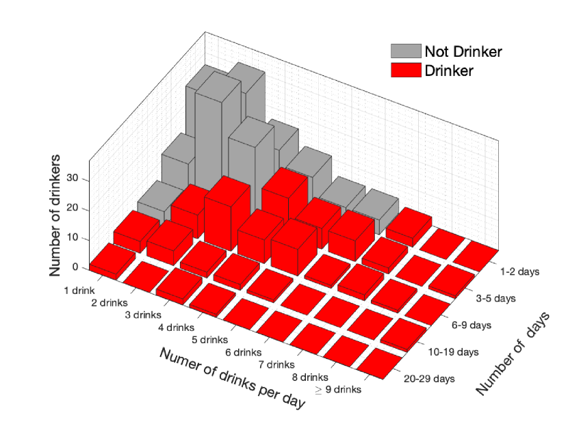
(a) Drinking behavior of participants

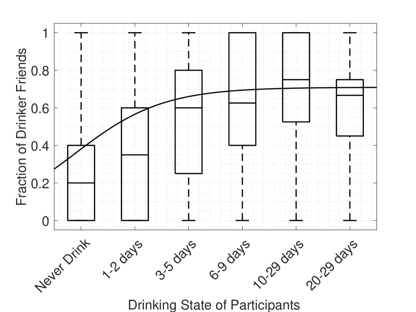
(b) Drinking behavior of participants and their friends

Figure 1: Drinking behavior of participants and their friends: The left panel is the two dimensional distribution of drinking state of participants who drink at least once in the last $30$ days, the red bars are drinker participants (based on definition of drinker in [42]). Including participants who have never drank, the result shows around $20\%$ of participants are drinkers. The right panel is the correlation between drinking status of all participants and their friends, the y-axis it the fraction of drinker friends (based on the participants perception of drinker) and the solid curve is the fitted curve to median revealing of the existence of a tipping point, that is, for non or light drinkers, people who drink more have more drinker friends, but for heavy drinkers the fraction of drinker friends saturate to a fixed value of $70\%$.

Beside that demographic questions, participants were asked about the contexts they visit more often during the day. From this collected data, we found the four most visited contexts on the ASU campus as Library (including Hyden and Nobel), Memorial Union (MU), Sun Devil Fitness Center (SDFC), and dorms/off-campus housing (including three locations). Along with this, we have an extra context (called Others) that is every place but these four contexts. The Figure (2) shows bar plot of visiting places based on the frequency. Among these four selected contexts, MU is the most visited one as the probability of visiting this context for all of the participants is higher than the other contexts.

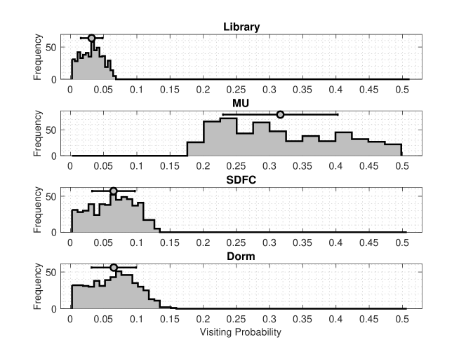
Figure 2: Per day visiting probability of visiting contexts: Each plot is the histogram for the number of participants (y-axis) who visit the specific context with per unit time probability (x-axis). The circle on the top of plots is the mean of the data and the line passing mean shows the first and third quartiles of the data. For instance $50$ participants visit MU with probability of $0.3$ and average probability of visiting MU for all participants is around $0.33$. MU is the most crowded location as its probability of visiting is higher than the other three contexts

.

2.1.2 CART Analysis

Classification and Regression Trees (CART) analysis is a tree-based method used to make decision of how independent variables (predictor) explain dependent variables (target). The CART technique selects the most effective predictors and their interaction from a large number of variables. Here we addressed primary questions related to understanding of the raw data.

We used CART on our data to examine the association between alcohol drinking behavior measured by Setting, Drink per setting, and Drinking status (being a drinker or not) for all participant, the ones who live on campus area, and the ones who live off campus area. Our predictor variables are age, race, gender, the number of clubs belonged to, school year, and fraction of drinker friends. We summarize the all target and predictors variables in Table (3).

	Symbol	Type	Description
	Setting	Qualitative	Number of days used alcohol in the last month: 1-2 days, 3-5 days, 6-9 days, 10-19 days, 20-29 days
Target	Drink.per.Setting	Integer	Number of drinks per day $\in\{0,...,8,9^{+}\}$
Variables	Drinking Status	Qualitative	Drinker, Not Drinker
	Age	Integer	Age of the participant
	Gender	Qualitative	F (Female), M (Male)
Predictor	Race	Qualitative	A(Asian), AA (African American), W(White), HL (Hispanic/Latino),
Variables			AIAN (American Indian or Alaska Native), M (Mixed), O (Other)
	School.Year	Qualitative	F(Freshman), SO (Sophomore), J(Junior), SN (Senior), G (Graduate)
	Club	Integer	The number of clubs participant belongs to $\in\{0,...,5\}$
	Drinker.Friends	Continuous	The fraction of drinker friends $\in[0,1]$

Table 2: The definition of variables used for CART analysis

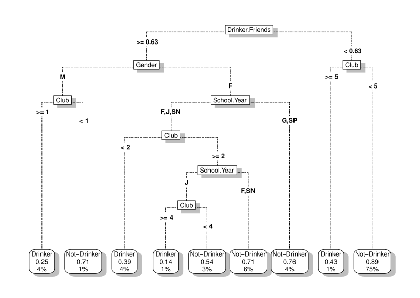
(a) Drinking Status for all $538$ participants

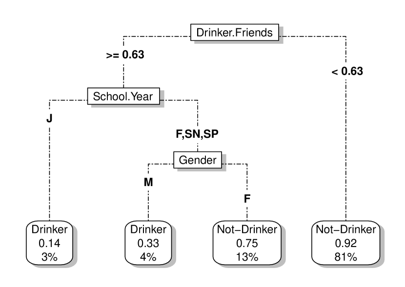
(b) Drinking Status for $269$ participants who live on campus

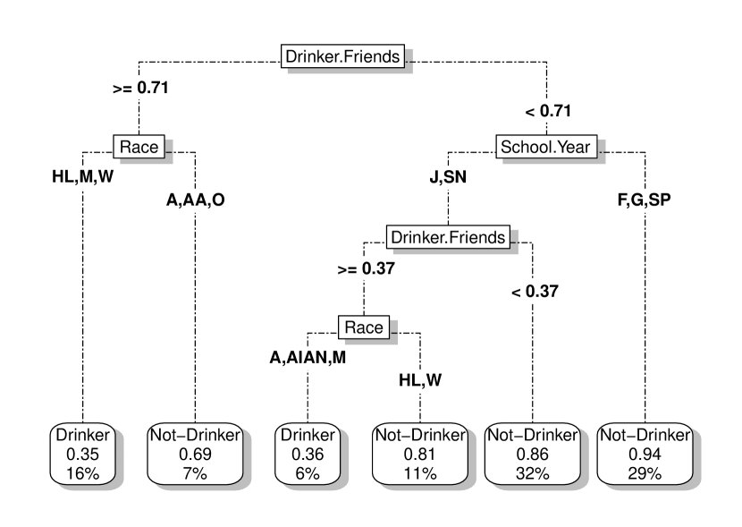
(c) Drinking Status for $267$ participants who live off campus

Figure 3: The output of CART analysis: This plot includes the decision tree for drinking status for all participants (3(a)), participants who live on campus (3(b)), and participants who live off campus (3(c)). The last row of each tree represent the terminal nodes (clusters). Each terminal node includes the predicted drinking status (drinker or not-drinker), the probability of being not-drinker, and the percentage of root sample size belonging to the corresponding category. For example based on the left terminal node in Subfigure (3(a)), $4\%$ of all participants are male who attend at least one club and more than $63\%$ of their friends are drinker. The probability of being not-drinker for these people is $0.25$, therefore, they are predicted as drinker.

Target	Cluster	Description
Variable	Number
	$3$	Sixty one percent of the participants have less than $45\%$ of their friends as drinkers, but themselves never drink.
	$4$	Thirty percent of participants have more than $45\%$ drinker friends but do not belong to $10\%$ of US race such as Asian and Pacific Islander and Native Hawaiian. They drunk for on an average of 3-5 days during past month.
Setting	$11$	Four percent of participants have more than $45\%$ drinker friends, are in minority race, and are in first, second or last year of their program. They, on average, never drunk during past month.
	$20$	Three percent of participants have more than $45\%$ drinker friends, are in minority race, and are and third year of their program. They, on average, drunk 1-2 days during past month.
	$21$	Three percent of participants have more than $45\%$ drinker friends, are in minority race, and are in fourth year of their program. They, on average, drunk 3-5 days during past month.
	$2$	Two percent of the participants are younger than $18$ years old and on average drunk $1.2$ times per setting during past month.
	$6$	Thirty percent of participants are older than $18$ years old and belong to Asian, African American, Mixed or Other races. They drunk for $3.4$ times per setting during past month.
	$14$	Twelve percent of participants are older than $18$ years old and belong to minority or White races and attend at most one club. They drunk for $3.3$ times per setting during past month.
	$30$	Thirty eight percent of participants are older than $18$ years old and belong to minority or White races and attend more than one club and more than $10\%$ of their friends are drinker. They drunk for $3.9$ times per setting during past month.
Drink.Per.Setting	$62$	Six percent of participants are between $18$ and $19$ years old and belong to minority or White races and attend more than one club and less than $10\%$ of their friends are drinker. They drunk for $3.7$ times per setting during past month.
	$126$	Six percent of participants are older than $20$ years old and belong to minority or White races and attend more than one club and less than $10\%$ of their friends are drinker. They drunk for $4.1$ times per setting during past month.
	$254$	Five percent of participants are between $19$ and $20$ years old and belong to minority or White races and attend more than one and less than three club and less than $10\%$ of their friends are drinker. They drunk for $5.7$ times per setting during past month.
	$255$	Two percent of participants are between $19$ and $20$ years old and belong to minority or White races and attend more than three clubs and less than $10\%$ of their friends are drinker. They drunk for $9.4$ times per setting during past month.

Table 3: A summary of result of CART analysis for various target variables

The Figures (3) show the trees reproduced by CART for the target variable Drinking Status. We interpret one of them in details, Subfigure (3(b)) and then interpretation of the rest would be similar. For the other target variables, we summarize the result in Table (3).

The Subfigure (3(b)) shows the tree reproduced by CART for Drinking status of participants living on campus as a qualitative variable. The tree has four terminal nodes with Drinker.Friend and School.Year are the primary splitters in the tree. That is, these predictors are critical in classifying drinking status. On the top of the tree (node 1), we have Drinker.Friends, therefore, the single best predictor to classify Setting is fraction of drinker friends. CART further directs the participants having more than $63\%$ of their friends as drinker to the left forming decision node 2, and directs the rest to the right forming terminal node 3. As indicated by this terminal node, if less than $63\%$ of friends are drinker, the tree predicts that the participant most likely never drinks ( $92\%$ out of $81\%$ of all data in this split). CART further splits node 2 based on participant’s School.Year and directs it with $J$ to the left, forming terminal node 4; directs the rest to the right, forming decision node 5. Terminal node 4 predicts that on average involved participants are drinker. CART continues to split node 5 based on gender into decision node 10 and terminal nodes 11. Terminal nodes 10 and 11 indicate that conditioned on having more than $63\%$ of friends as drinker, being Freshman, Senior or sophomore and being female, the participant most probably are not drinker( $75\%$ out of $13\%$ of all data in this split), but being male, he most probably is drinker ( $100\%-33\%=67\%$ out of $4\%$ of all data in this split).

For all of these trees the fraction of drinker friends plays an important role on drinking behavior of participants that this finding is consistent with the analysis results shown in Subfigure (1(b)), and many other studies such as [43, 44]. Other relatively significant factors driving alcohol behavior are Race, School.Year and Club. There is no control on Race or School.Year, nevertheless, Drinker. Friends and Clubs can be representative of level of socializing and its indirect impact (supported by our CART analysis) on alcohol drinking behavior[45]. Various contexts within university campus provide various amount of opportunity to socialize and therefore various risk of becoming an alcohol drinker. The topic of our next Subsection is to measure this indirect impact of socializing context via developing an ABM.

2.2 Agent Based Model

ABMs- computer based models- simulate the actions and interactions of autonomous agents representing the individuals of the modeled population. The short- and long- term activity of the agents can be compiled to obtain population-level measures of a biological system at a given scale [46]. Here we create an agent-based stochastic model (ABM) in which students are classified based on their drinking status and college social context. To explain our model we follow the structure in [47] called ODD (Overview- Design concepts-Details) protocol.

2.2.1 Overview

Purpose: The purpose of the model is to understand how spending time at different locations of university campus (called contexts) affects the dynamics of drinking behaviour among students.
 
State variables and scales: The model comprises three hierarchical levels: environment (campus geographical area), context (social activities/events), and individuals (students).

• The environment resembles the campus area, which is around $660$ acres $4\times 4$ grid from Rail road-Rural road in South East to University Dr–Fifth avenue in North West, Figure (4).

  

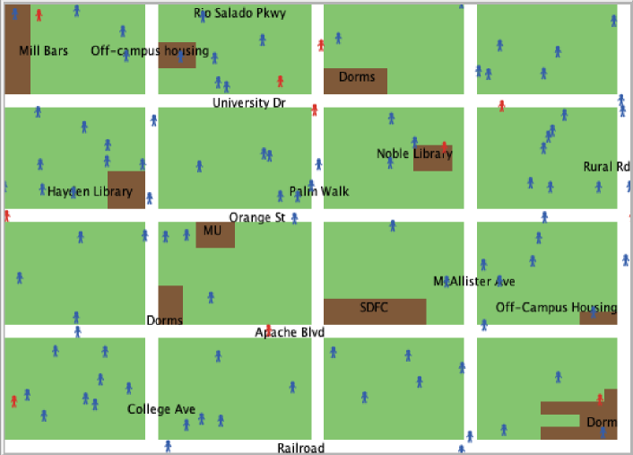
  Figure 4: The map of ASU campus and spatial instance of simulation: Four main contexts are the brown patches, and the rest is other area.

  This environment includes several contexts -an specific location of university campus - in where individuals move around and interact.

• The contexts are listed as

  1. Library: that includes two different libraries, Hyden that is the largest and most visited library facility at ASU, and Nobel library.

  2. Memorial Union (MU): considered as living room of campus. This context provides students with different experience activities such as student organization, community service, planning an event or eating meal.

  3. Sun Devil Fitness Complex (SDFC): also known as Physical Education West and is used mostly for intramural sports at the campus.

  4. Dorms: that are parts of Campus Housing. There are several residence halls (dorms) in Tempe campus.

  5. Other places: We assume if individuals are not spending time in the previous mentioned contexts, they are in other places shown in Figure (4) as long as they are in campus.

  These contexts are selected and labeled as $C_{1}-C_{5}$ as they are the most crowded contexts that individuals gather at events or collective activities, therefore, they are closer to each other rather than when they just move at random. Each context named $C_{i}$ for $i\in\{1,..,5\}$ is characterized by three attributes. The first attribute is the constant probability of contact between two typical individuals visited context $C_{i}$, $\sigma_{C_{i}}$. To find this parameter, we used a very ad hoc approach assuming this probability is density-based with a power proportion behavior, that is, we define $\bar{N}_{C_{i}}$ as per area average number of individuals visiting context $C_{i}$, then we have

  $$\sigma_{C_{i}}=\frac{\sqrt{\bar{N}_{C_{i}}}}{\sum_{j=1}^{4}\sqrt{\bar{N}_{C_{j}}}},~{}~{}i=1,\cdots,4,$$ (1)

  and for the last context $C_{5}$, we assume $\sigma_{C_{5}}=0$, that is, for the places other than the first four no contact causing to spread of drinking behavior happens. The function (1) is selected to represent an intermediate between frequency- and density-dependence contacts [48], with the square root that provides a saturating shape. Assuming the area of all four contexts under study is the same, we use the normalized mean probability of visiting context $C_{i}$ called $p_{C_{i}}$ (the circle points in Figure (2)) and multinominal distribution to find $\bar{N}_{C_{i}}=Np_{C_{i}}$ as the average number of individuals located in context $C_{i}$. The second attribute is constant probability of drinking behavior transmission within one contact happened at $C_{i}$. We call this probability as drinking influence success $\beta_{C_{i}}$, which provides the chance that a drinker spread his/her behavior to others via a contact. The last attribute is an state variable of the number drinkers visited context $C_{i}$ at time $t$, $I_{C_{i}}(t)$. These attributes for context $C_{i}$ are shown by $\theta_{C_{i}}(t)=(\sigma_{C_{i}},\beta_{C_{i}},I_{C_{i}}(t))$

• We consider $N=538$ (survey sample size) ASU college students in our ABM. An individual (i.e., a typical student) in this cohort is represented by $\textbf{A}_{i}$, $i\in\{1,..,N\}$, who is characterized by four attributes (some of them may change over time):

  • Class-year, $R_{i}$: $0$ (Freshman), $1$ (Sophomore), $2$ (Junior), $3$ (Senior), and $4$ (Graduate),

  • Probability of visiting a contexts, $P_{i}$, (the $i^{th}$ row of the following matrix):

    $$\mathcal{P}_{N,n}=\begin{pmatrix}P_{1}(C_{1})&P_{1}(C_{2})&\cdots&P_{1}(C_{n})\\ \vdots&\vdots&\vdots&\vdots\\ P_{i}(C_{1})&P_{1}(C_{2})&\cdots&P_{i}(C_{n})\\ \vdots&\vdots&\vdots&\vdots\\ P_{N}(C_{1})&P_{N}(C_{2})&\cdots&P_{N}(C_{n})\end{pmatrix}.$$

    The matrix $\mathcal{P}_{N,n}$ is designed and estimated based on our survey data. Hence, the matrix dimension is $538\times 5$ where $P_{i}(C_{k})$ entry is the probability of an individual $\textbf{A}_{i}$ to move to a context $C_{k}$,

  • the context that the individual $\textbf{A}_{i}$ is at time $t$, $V_{i}(t)$: (e.g., for our modeling population $V_{i}(t)\in\{C_{1},C_{2},C_{3},C_{4},C_{5}\}$, $\forall t$), and

  • drinking state $S_{i}(t)$, ($S_{i}(t)\in\{ND,D,FD\}$, $\forall t$)): The three states are $ND$ (representing non-drinker individual who may be susceptible to initiating drinking behavior [31]), $D$ (stands for current drinker, defined based on [42] (see Subsection (2.1.1))), and $FD$ (stands for former drinker who were drinker before [49]).

  To summarize, we define an attribute $\eta$ for individual $\textbf{A}_{i}$ as $\eta_{i}(t)=(R_{i}(t),P_{i},V_{i}(t),S_{i}(t))$. For example $\eta_{i}(t)=(0,[0.14,0.06,0.41,0.24,0.15],C_{k},ND)$ means that non-drinker freshman individual $\textbf{A}_{i}$ has a $14\%$ chance of of being in context $C_{1}$, $6\%$ chance in context $C_{2}$ and so on, but currently he/she is at context $C_{k}$.

Process overview and scheduling: The model proceeds in two hours (1 tick) time steps with the assumption that a day is 16 hours (7am-11pm), or 8 ticks. Within each tick proceeding phases are ordered as follow: individuals movement to various contexts, drinking behavior transmission, recovery from drinking, drinking reinitiation at individuals’ discretion, and class-year updates at the end of each $1440$ ticks (corresponding to one academic year or 9 months). At the end of academic year graduate students leave the school, but for each one graduate individual who leaves the school, we introduce a new freshman who is non-drinker, but all other their characteristic is the same as left one, therefore, the total number of individuals is conserved during the simulation. Within each phase, individuals are processed in a random order. The phases are depicted in Figure (5).

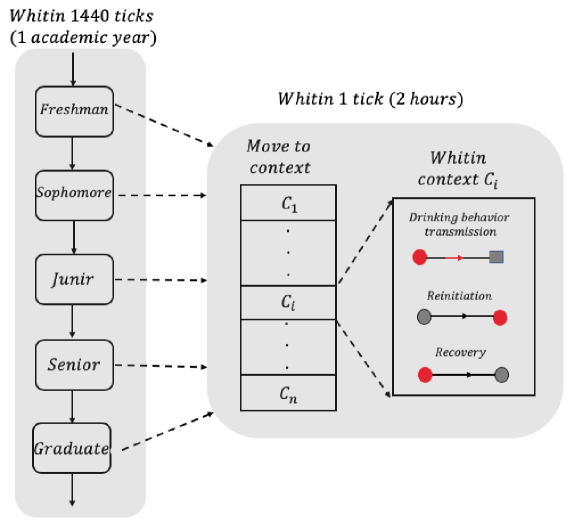
Figure 5: Model phases: Four phases are proceeding in every tick, and c phase is updated in every $1440$ tick.

2.2.2 Design concepts

Emergence: Total population dynamics emerge from the processes of update class-year. Transmission dynamics, however, partially emerges from the processes of movement and contacts. The number of individuals leaving drinking state or reinitiate drinking does not depend on the time but is drawn from a proper distribution that was observed in field studies, see Section (2.2.3).
 
Stochasticity: All movements, interactions and behavioural parameters are interpreted as probabilities, some drawn from empirical probability distributions captured from data, while the rest are taken from some predetermined distributions. To summarize, the stochasticity of model is the result of (a) movement to typical context $C_{i}$, (b) making contact with non-drinker and or former drinker and transmit drinking behavior by drinker, (c) reinitiang drinking by former drinker at their discretion, and (d) recovery from drinking state by drinker. The Table (6) in Appendix list all the random variables in our ABM and their corresponding distribution.

Observation: To test our model, we observe the spatial distribution of individuals, and to analyse the model, we record context-related stochastic parameters and population-level variables, i.e. group size distribution, time series of population size with various alcohol-related states: non-drinker, drinker, and former drinker.

2.2.3 Details

Initialization: At initial time we randomly select $30\%$ as freshman, $25\%$ as sophomore, $23\%$ as junior, $18\%$ as senior and $4\%$ as graduate. We also randomly select $5\%$ of population as drinker and assume the rest are non-drinker. At the beginning of every $8$ ticks (every day), individuals are placed randomly in the environment. Each model simulation was run up to reaching quasi-stationary state for $200$ replicates.
 
Input: For the base simulation, the input parameters and probabilities were set so that the model fits reported data and filed study. The total number of individuals $N=538$, total number of contexts $n=5$, and movement probability vector of each individual is taken from survey data. Some drinking spread parameters (reinitiate drinking behavior $\rho$, leaving drinking $\gamma$) were found in literature [31, 50, 51]. The context influence rates $\beta_{C_{i}}$ are parameterised to resemble to current prevalence of drinking as a quasi-stationary state, that is, we calibrated these parameters to the current $20\%$ fraction of drinkers. The Table (4) list the input parameters, their definition and baseline values.

Notation	Definition	Baseline	Ref.
$\beta_{Library}$	Drinking influence success at Library	$0.0105$	Calibrated
$\beta_{MU}$	Drinking influence success at MU	$0.0033$	Calibrated
$\beta_{SDFC}$	Drinking influence success at SDFC	$0.0073$	Calibrated
$\beta_{Dorm}$	Drinking influence success at Dorm	$0.0074$	Calibrated
$\sigma_{Library}$	Contact probability at Library	$0.1429$	Survey data
$\sigma_{MU}$	Contact probability at MU	$0.4492$	Survey data
$\sigma_{SDFC}$	Contact probability at SDFC	$0.2043$	Survey data
$\sigma_{Dorm}$	Contact probability at Dorm	$0.2037$	Survey data
$\rho$	Reinitiation drinking at discretion probability	$0.0187$	[31, 50, 51]
$\gamma$	Recovery from drinking probability	$0.0187$	[31, 50, 51]

Table 4: Parameters definition and baseline value: The model parameters describing the drinking behavior dynamic that are estimated using survey data, or calibration method explained in Subsection (3.1), and or obtained from the literature.

Submodels:

Movement: Through time individuals move in the five different contexts within the environment. Each tick and for a typical individual $\textbf{A}_{i}$ with predetermined probability vector $P_{i}$, we generate random number $u\in[0,1]$. Then if

$$\sum_{j=1}^{m-1}P_{i}(j)<u\leq\sum_{j=1}^{m}P_{i}(j),$$

for some $1\leq m\leq n$, then we place $\textbf{A}_{i}$ in context $C_{m}$.

For drinking behavior dynamic within any context we borrow the model in [31] shown in Figure (6).

Variable	Definition
$ND$	Non-drinker defined based on [31].
$D$	Drinker defined based on [42].
$FD$	Former drinker defined based on [49].

Figure 6: Role governing drinking behavior spread and variables definition.

This model includes three processes explained below:

Drinking behavior transmission: On each tick, we model the ability for a drinker individual to spread his/her behavior to other non-drinker or former drinker visiting at the same context as follow:

$$\begin{aligned} ~{}~{}~{}=~{}~{}~{}~{}~{}~{}~{}~{}~{}~{}~{}~{}~{}~{}~{}~{}&\sigma_{C}~{}~{}~{}~{}~{}~{}~{}~{}~{}~{}~{}~{}~{}~{}~{}~{}~{}\times~{}~{}~{}~{}~{}~{}~{}~{}~{}~{}~{}~{}~{}~{}~{}~{}~{}~{}~{}~{}\beta_{C}~{}~{}~{}~{}~{}~{}~{}~{}~{}~{}~{}~{}~{}~{}~{}~{}\times~{}~{}~{}~{}~{}~{}~{}~{}\left(1-\phi\right),\end{aligned}$$

where the resistancy $\phi$ is a measure for combination of susceptibility level of non-drinker or former drinker individual toward drinking behavior and infectivity level of drinker individual. Because in real world, not all non-drinker or former drinkers are equally likely to become drinkers, and not all drinker are equally likely to transmit their behavior. Although the susceptibility of an individual may depends on its drinking state ( non-drinker or former drinker), for simplicity we assume non-drinker and former drinker both have the same susceptibility level. With all these assumptions, we assume resistancy $\phi$ follows a uniform distribution in $[0,1]$, that is, for each contact between a drinker and non-drinker (former drinker) individuals we assign a uniform random number where closer to zero means the contact is less resistant and drinking behavior more likely to be transmitted and vice versa [34].

The aggregated probability that a typical non-drinker individual $\textbf{A}_{i}$ who visits context $C_{k}$ become drinker is

$$P(S_{i}(t+\Delta t)=D | S_{i}(t)=ND~{}\&~{}V_{i}(t)=C_{k})=1-\left[1-\sigma_{C_{k}}\beta_{C_{k}}(1-\phi)\right]^{I_{C_{k}}(t)}.$$

Therefore, the probability that non-drinker $A_{i}$ become drinker within time step $\Delta t$ is

$$\lambda(t) =P(S_{i}(t+\Delta t)=D|S_{i}(t)=ND)=\sum_{k=1}^{5}P(S_{i}(t+\Delta t)=D|S_{i}(t)=ND~{}\&~{}V_{i}(t)=C_{k})$$

$$=\sum_{k=1}^{5}1-\left[1-\sigma_{C_{k}}\beta_{C_{k}}(1-\phi)\right]^{I_{C_{k}}(t)}.$$

The former drinker has two reason to become drinker: Transmission or Reinitiation at discretion. The aggregated probability of becoming drinker via transmission for a typical former drinker $\textbf{A}_{i}$ who has not reinitiated drinking at his/her discretion but visits context $C_{k}$ is

$$\begin{aligned} P(S_{i}(t+\Delta t)=D&|&S_{i}(t)=FD~{}\&~{}V_{i}(t)=C_{k}~{}\&~{}\text{Transmission})=1-\left[1-\sigma_{C_{k}}\beta_{C_{k}}(1-\phi)\right]^{I_{C_{k}}(t)}.\end{aligned}$$

Reinitiation at discretion: The former drinker individual $\textbf{A}_{j}$ who has not received drinking behavior by a drinker may start drinking independent of environment with probability

$$\begin{aligned} P(S_{i}(t+\Delta t)=D&|&S_{i}(t)=FD~{}\&~{}\text{Re-initiation at discretion})=\rho.\end{aligned}$$

That is, the total probability that former drinker $A_{i}$ become drinker within time step $\Delta t$ is

$$P(S_{i}(t+\Delta t)=D|S_{i}(t)=FD)=\left\{\begin{array}[]{ll}\lambda(t)&\textnormal{ Re-initiation due to Transmission}\\ \rho&\textnormal{ Re-initiation at discretion.}\\ \end{array}\right.$$

Leaving drinking state: For a given drinker individual $\textbf{A}_{k}$ the random variable $T_{k}>0$ is defined to be the time at which the $\textbf{A}_{k}$ changes its status to former drinker. This is modelled as being exponentially distributed so that the average time to recover is $\frac{1}{\gamma}.$ It then follows that $T_{k}$ is memoryless (probability that a drinker leaves drinking status to former drinker is the same at each increment of time) and

$$P(T_{k}<\Delta t)=1-e^{-\gamma\Delta t}.$$

We summarized all parameters of ABM in Table (7) and its full model process for a single tick $\Delta t$ in pseudocode (1) in Appendix.

3 Results

In this Section we carry out local and global sensitivity analysis to evaluate the impact of context-related parameters involved in the model on drinking prevalence. Each simulation is average of a bunch of single realizations of stochastic ABM explained in Section 2. All of the realizations start at the same initial point obtained with the model baseline parameters in Table (4), unless stated otherwise.

3.1 Model initialization

We initialize our model based on estimates for the current drinking epidemic among ASU students in Tempe campus. The $5\%$ initial drinkers are randomly distributed in an otherwise non-drinker population. They are distributed as they would be as part of an emerging epidemic that started sometime in the past.

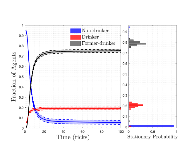
Figure 7: Time series of fraction of agents with different status: (Left) The fractions for average of $1000$ different stochastic simulations (solid curve) $\pm$ two standard deviations (dashed curve) of non-drinkers (blue), drinkers (red), and former drinkers (black). The influence rate within contexts $\beta_{C}$ are selected so we reach around $20\%$ (Mean =0.1923; 95% CI (0.1785, 0.2061) ) prevalence of drinkers at quasi-stationary state. (Right) The stationary distributions of fractions with different status for $1000$ simulated sample paths (histograms).

In order to estimate unknown drinking influence success parameter, $\beta_{C_{i}}$, we calibrate transmission probability to the current drinking prevalence using Method of Simulated Moments (MSM) [52]. We define context related transmission probability as $\tilde{\beta}_{C_{i}}=\sigma_{C_{i}}\beta_{C_{i}}$, and assume this parameter is the same for all contexts. We, therefore, choose the unknown parameter as $\tilde{\beta}=\sigma\beta$ and the first moment, mean of the prevalence at quasi-stationary state, as $20\%$ of drinkers, which is estimated based on the survey data explained in Section 2. After finding the optimized value $\tilde{\beta}$, the reported drinking influence successes in Table (4) are defined as

$$\beta_{C_{i}}=\frac{\tilde{\beta}}{\sigma_{C_{i}}}.$$

The Figure (7) illustrates the typical progression of the drinking behavior to reach the current prevalence of $20\%$ drinkers among colleague students in Tempe campus, ASU.

3.2 Sensitivity analysis

One set of the parameters in the model with less precise estimation is context related parameter: contact probability at context $\sigma_{C}$ and drinking influence success $\beta_{C}$. Combining these two parameters, we define transmission probability at context $C$ as $\tilde{\beta}_{C}=\sigma_{C}\beta_{C}$ and select it as inputs for the Sensitivity Analysis (SA), which is called Parameter of Interest (POI). As Quantity of Interest (QOI) we select fraction of drinkers at quasi-stationary state.

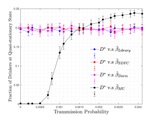
Figure 8: Local SA on transmission probability at different contexts (the x-axis) against drinking prevalence at quasi-stationary state (y-axis): The curve corresponding to context $C$ is the plot of fraction of drinkers at quasi-stationary state (y-axis $=D^{*}$) as the transmission probability of corresponding context (x-axis $=\tilde{\beta}_{C}$) changes while the transmission probability for the other contexts than context $C$ are constant at their baseline value. The drinking prevalence are averaged over the $200$ simulations with reported $95\%$ confidence intervals. While transmission probability in other contexts does not effect drinking prevalence, the transmission probability for MU is highly effective. The retardation in growth rate in MU indicates the assumption of sigmoidal pattern: when $\tilde{\beta}_{MU}$ is big enough, that is for $\tilde{\beta}_{MU}\geq 0.001$ drinking prevalence increases rapidly and level of at its plateau of around $25\%$.

Conducting the pretest of $1000$ runs at parameter values defined at baseline and recording output at every tick, we observed that from $t=50$ to $t=100$ the number of drinkers have stabilised with some random fluctuations around its mean, Figure (7). Therefore, we used that $50$ ticks as the reasonable time period for the sensitivity analysis [53].

We first conducted a local SA on POIs by changing one parameter at a time to evaluate their impact on the QOI. That is, over its reasonable range we vary one POI- while keeping other parameters at their baseline value- and observe its impact on QOI. Using NetLogo’s Behavior Space feature we programmed a series of parallel runs with a given range of parameter values, to carry out local sensitivity. In a given set of simulations, the code was run for a transmission probability at a context $C$ in $[0,2\tilde{\beta}_{C}]$ per tick. The reported result in Figure (8) is the average of $200$ simulations. In all contexts except MU the QOI is almost unchanged as POI increases in its range. But the nonlinear effect in the experiment for MU is evident of the logistic-shaped curve: there is a tipping point below which increasing transmission probability does not affect drinking prevalence drastically, and above which transmission probability would bring the drinking behavior outbreak stabilizes at $25\%$. The local SA for our model indicates that $\beta_{MU}$ is by far the most effective parameter for resulting an outbreak or bringing the epidemic under control. The reason is that the density of the population in this context is higher than the other contexts, Figure (2).

We then used nlrx package in R [54] to conduct two different global SA: Regression-based method and Variance-based Sobol methods.

Regression-based method: Assuming monotonicity between inputs and output, Partial Correlation Coefficient (PCC) and Standard Regression Coefficients (SRC) are reliable methods that provide a measure of this monotonicity [55]. With the assumption that there is no correlation between POIs, PCC measures the degree of correlation between QOI and one POI by removing the effect of other POIs on QOI [56]. SRCs are the coefficient for the regression model that are taken from standardised POIs and QOI[56]. Therefore, higher values for PCC and SRC indicates more sensitivity to the corresponding POI.

We combined these regression methods with Latin Hypercube Sampling (LHS) [55, 57] to conduct an SA on our model output. Via LHS sampling, we selected $1000$ samples from a uniform distribution of the POI ranges in $[0,2\tilde{\beta}_{C}]$ for all four contexts and run the model for each sample to calculate PCCs and SRCs for QOI, the Table (5). Similar to local SA, the result indicates that transmission probability in MU is highly sensitive parameter with its index is around $0.8$ for both PCC and SRC, while the values for other contexts is almost negligible. Producing the same rankings for PCC and SRC is the result of the assumption of no correlation imposed on the POIs [58].

Variance-based method: Despite being costly in computation, Sobol method is a model-free variance-based method capable of quantifying the effect of POIs and their interaction on the variance of QOI with the assumption that POIs are independent [59].

We carried out Sobol SA using nlrx package for a total sample size of $1000$ runs, sampled from uniform distributions in the range $[0,2\tilde{\beta}_{C}]$. We used bootstrap confidence intervals for $100$ bootstrap samples to assess the accuracy of the estimated sensitivities. The resulting main effect and total-order indices with their $95\%$ confidence intervals are shown in Table (5). A number of confidence intervals contains negative values that are biologically meaningless but are the result of numerical inaccuracy of the method [59]. We could have discarded these negative ranges by setting negative indices equal to zero but it triggers a bias in bootstrap confidence interval, so we kept negative values. The sum of all main effect indices is $0.81$, that means more than $80\%$ of drinking prevalence variance is explained by sole impact of transmission probabilities and less than $20\%$ explained by their interaction. The total order indices indicate that all the mentioned ineffective parameters in previous Sections contribute to a tangible variance after including interaction effects. Additionally, the parameters have wide confidence intervals (order of magnitude $-1$) showing that their estimate needs to be improved by increasing the number of bootstrap samples. Finally, similar to previous results in SA, $\tilde{\beta}_{MU}$ is the most sensitive parameter as its main effect and total order indices are larger than those of other parameters.

	Regression-based Method		Variance-based Method
	PCC (95% CI)	SRC (95% CI)	Main Effect (95% CI)	Total Order (95% CI)
$\tilde{\beta}_{Dorm}$	$0.098$($[0.028,0.158]$)	$0.042([0.016,0.069])$	$0.043$($[0.000,0.086]$)	$0.182([-0.018,0.210])$
$\tilde{\beta}_{Library}$	$-0.040([-0.098,0.023])$	$-0.017([-0.039,0.005])$	$0.041$($[0.000,0.081]$)	$0.172([-0.037,0.246])$
$\tilde{\beta}_{MU}$	$0.905([0.888,0.924])$	$0.890[(0.866,0.913])$	$0.695([0.683,0.706])$	$0.832([0.744,0.889])$
$\tilde{\beta}_{SDFC}$	$0.076([0.002,0.129])$	$0.032([0.008,0.058])$	$0.041([0.000,0.083])$	$0.175([-0.022,0.226])$

Table 5: Sensitivity ranking of Partial Correlation Coefficients (PCC) and Standard Regression Coefficients (SRC) and Main effect and total order Sobol indices for for transmission probabilities: Ten replications of a LHS design with $1000$ samples was simulated for run time of $100$ ticks for each simulation. Transmission probability in MU, $\tilde{\beta}_{MU}$, is the most sensitive parameter, while transmission probability in other contexts has almost no impact on the fraction of drinkers at quasi-stationary state. Ten replications of a Sobol design with $1000$ samples and $100$ bootstrap samples was simulated for run time of $100$ ticks for each simulation. Transmission probability in MU, $\tilde{\beta}_{MU}$, is the most sensitive parameter, and transmission probability in other contexts play a role on the fraction of drinkers at quasi-stationary state when they interact with other parameters.

4 Discussion

We used and analyzed the collected data of demographic characteristics, alcohol drinking behavior, and daily activity of students and designed an Agent-based model to understand social behavioral mechanisms that drive drinking patterns at the Arizona State University (ASU) students community. Our model tracks the movement and interaction of a population of non-drinker, drinker and former drinker agents on a 2-dimensional lattice environment including several patches that resemble different contexts of university campus. Non-drinker agents became drinker on the basis of “context-influence” implemented in terms context related transmission probability, which is a combination of probability of contact and drinking influence success at any given context. A former drinker agent has also context-influence reasoning plus internal tendencies to become drinker again. And finally the drinker stops drinking after passing a certain drinking period.

Our data analysis on the sample of collage aged students at ASU confirmed the presence of significant peer influences (via drinker friends) as well as show how high socialization within various (and even non-drinking) social contexts impacts drinking dynamics in the simulated population, Figures (1 and 3). Throughout our modeling study, we have focused on the effects of environmental factors to drinking behavior of ASU students. We linked the social mixing behavior (in non-drinking) contexts to drinking patterns and found out governing factors on college drinking dynamic. Within this framework, the sensitivity analysis explicitly showed the role of time spent in a particular context on the dynamics of alcohol drinking. In particular, dynamics of college students drinking is primarily governed by high crowded contexts and the intensity of social mixing. However, the relationship between mixing intensity in social contexts and drinking patterns, is non-trivial and our result (through use of ABM) suggests that drinking pattern follows a logistic trend. Specifically, local sensitivity analysis showed us that there is a threshold transmission probability at which non-drinkers converted to drinkers most efficiently if they spend more time in the most crowded context, Figure (8).

The findings of our model study needs to be understood in terms of the several limitations. First, our parametrization and calibrations of model parameters are subject to limited sample size of the data. Second, ABMs in nature are challenging when applied to understand interaction of agents ignoring highly subjective and not necessarily rational behaviors in the system of social science [60]. Third, there may be high uncertainty in some of the considered parameters, which may depends on specific environment and context. Fourth, because the main goal of this study was to understand the role of environment influences on alcohol drinking behaviors, we ignored many other factors (such as age, race, or gender) that may be linked to drinking. Future research should carefully measure these factors and capture their impact via an ABM coupled with social network framework constructed based on the correlations between the number of friends a person has and his/her daily activity within the campus. This social network should be characterized by ages, ethnicity, social groups, and geographic location. Although the model is still too simple to directly guide intervention efforts, the qualitative trends predicted by these simulations can be useful in designing studies to quantify the effectiveness of different intervention approaches.

Appendix

Random Variable	Value	Implications
$P_{i}(C_{k})$	Empirical distribution	Prob that individual $A_{i}$ moves to context $C_{k}$.
$\phi$	Uniform (0,1)	Resistency: susceptibility level of non- or former drinker times infectivity level of dinker.
$\sigma$	Bernoulli($\sigma_{C_{k}}$)	Prob of making contact between two individual visiting context $C_{k}$.
$\beta$	Bernoulli ($\beta_{C_{k}}$)	Prob of drinking behavior transmission happens within one contact at context $C_{k}$.
$\rho_{i}$	Bernoulli($\rho$)	Prob of alcohol drinking reinitiation at discretion for former drinker $A_{i}$.
$T_{i}=1/\gamma_{i}$	Exponential($\gamma$)	Duration of drinking behavior for drinker $A_{i}$.

Table 6: Random variables used in ABM algorithm and their corresponding distributions.

	Symbol	Definition	Range
	n	Total number of socializing contexts.	–
Context	$\sigma_{C_{i}}$	Prob. of contact between two individuals visited context $C_{i}$.	$[0,1]$
Agent	$\beta_{C_{i}}$	Prob. of drinking behavior transmission per contact at $C_{i}$.	$[0,1]$
Parameters	$I_{C_{i}}(t)$	The number of drinkers at context $C_{i}$ at time $t$.	$\{0,1,\cdot\cdot\cdot,N\}$
	$\bar{N}_{C_{i}}$	Per area average number of individuals visiting context $C_{i}$.	–
	$p_{C_{i}}(t)$	Mean proba. of visiting context $C_{i}$.	$[0,1]$
	$N$	Total number of individuals.	–
Individual	$R_{i}(t)$	class-year of individual $A_{i}$ at time $t$.	$\{0\textnormal{(Freshman)},1\textnormal{(Sophomore)}$
Agent			$2\textnormal{(Junior)},3\textnormal{(Senior)},4\textnormal{(Graduate)}\}$
Parameters	$P_{i}$	Per tick prob. vector of visiting contexts by individual $A_{i}$. $P_{i}$ is a vector of size n where $k^{th}$ element ($P_{i}(C_{k})$ ) is the chance that individual $A_{i}$ visit context $C_{k}$.	$[0,1]^{n}$
	$V_{i}(t)$	The visited context of individual $A_{i}$ at time $t$: $A_{i}$ is at context $V_{i}(t)$ at time $t$.	$\{C_{1},\cdot\cdot\cdot,C_{n}\}$
	$S_{i}(t)$	Drinking state of individual $A_{i}$ at time $t$.	$\{ND,D,SD\}$
Alcohol	$\gamma$	Prob. of recovery from drinking.	$[0,1]$
Drinking	$\rho$	Prob. of re-initiation drinking at discretion.	$[0,1]$
Parameters	$\phi$	Resistancy: susceptibility of non- or former drinkers times infectivity of drinker.	$[0,1]$

Table 7: The set of all parameters and attributes defined in our ABM.

Notation	Description
$\textbf{A}_{k}$	An individual with ID k
$\eta_{k}(t)=(R_{k}(t),P_{k},V_{k}(t),S_{k}(t))$	Attribute of individual $\textbf{A}_{k}$ at time t
$S.add(m)$	Add element m to a set S
$DP(k)$	Drinking period for drinker individual $\textbf{A}_{k}$
$ern(a)$	Exponential random number with parameter $a>0$
$urn$	Uniform random number in $[0,1]$
$rem(a,b)$	Remainder after division of a by b

Table 8: Table of notation for a conventional model in algorithm.

1 $NC=\emptyset$ %$NC$ is an empty set.;

2 for $\textbf{A}_{k}$ with $\eta_{k}(t)=(R_{k}(t),P_{k},V_{k}(t),S_{k}(t))$ do

3      $\%==============$/*Movement*/$==============\%$;

4       $j=min\{m:urn\leq\sum_{i=1}^{m}P_{k}(i)\}$;

5       $V_{k}(t+\Delta t)\leftarrow C_{j}$ ;

6       if $S_{k}(t)=D$ then

7            $\%========$/*Drinking behavior transmission*/$========\%$;

8             for $\textbf{A}_{j}\in\{\textbf{A}_{i}\notin NC:V_{i}(t)=V_{k}(t),S_{k}(t)\neq D\}$ do

9                   if urn$\leq\sigma_{V_{k}(t)}\beta_{V_{k}(t)}urn$ then

10                        $S_{j}(t+\Delta t)\leftarrow D$,  $DP(j)\leftarrow-1$ ,   $NC.add(\textbf{A}_{j})$;

11                        

12                   end if

13                  

14             end for

15            $\%========$/*Recovery from drinking*/$========\%$;

16             if $DP(k)=-1$ then

17                  $DP(k)\leftarrow max\{\Delta t,ern(\gamma$)};

18                  

19             else if $DP(k)>0$ then

20                  $DP(k)\leftarrow DP(k)-\Delta t$;

21             else

22                  $S_{k}(t+\Delta t)\leftarrow FD$;

23             end if

24            

25       end if

26      $\%========$/*Reinitiation at discretion*/$========\%$;

27       if $S_{k}(t)=FD$ & $k\notin NC$ & $urn\leq\rho$ then

28            $S_{k}(t+\Delta t)\leftarrow D$,   $DP(k)\leftarrow-1$,  $NC.add(\textbf{A}_{k})$

29       end if

30      $\%========$/*class-year*/$========\%$;

31       if $rem(t,1440)=0$ then

32            $R_{k}(t+\Delta t)\leftarrow R_{k}(t)+1$;

33             if $R_{k}(t+\Delta t)=5$ then

34                  $R_{k}(t+\Delta t)=0$,  $S_{k}(t+\Delta t)=ND$

35             end if

36            

37       end if

38      

39 end for

Algorithm 1 The model dynamic at typical time $t$

References

- [1] Roisin M O’connor and Craig R Colder. Predicting alcohol patterns in first-year college students through motivational systems and reasons for drinking. Psychology of Addictive Behaviors, 19(1):10, 2005.
- [2] Kypros Kypri, John Langley, and Shaun Stephenson. Episode-centred analysis of drinking to intoxication in university students. Alcohol and Alcoholism, 40(5):447–452, 2005.
- [3] John W Fishburne and Janice M Brown. How do college students estimate their drinking? comparing consumption patterns among quantity-frequency, graduated frequency, and timeline follow-back methods. Journal of Alcohol and Drug Education, 50(1):15, 2006.
- [4] Jennifer L Burden and Stephen A Maisto. Expectancies, evaluations and attitudes: prediction of college student drinking behavior. Journal of studies on alcohol, 61(2):323–331, 2000.
- [5] Kenzie A Cameron and Shelly Campo. Stepping back from social norms campaigns: Comparing normative influences to other predictors of health behaviors. Health Communication, 20(3):277–288, 2006.
- [6] Cecile Dantzer, Jane Wardle, Ray Fuller, Sacha Z Pampalone, and Andrew Steptoe. International study of heavy drinking: Attitudes and sociodemographic factors in university students. Journal of American College Health, 55(2):83–90, 2006.
- [7] Edward A Malloy. Rethinking rites of passage: Substance abuse on America’s campuses. Center on Addiction and Substance Abuse at Columbia University, 1994.
- [8] David J Nutt, Leslie A King, Lawrence D Phillips, et al. Drug harms in the uk: a multicriteria decision analysis. The Lancet, 376(9752):1558–1565, 2010.
- [9] Bert Aertgeerts and Frank Buntinx. The relation between alcohol abuse or dependence and academic performance in first-year college students. Journal of adolescent health, 31(3):223–225, 2002.
- [10] Royce A Singleton and Amy R Wolfson. Alcohol consumption, sleep, and academic performance among college students. Journal of studies on alcohol and drugs, 70(3):355–363, 2009.
- [11] M Lynne Cooper. Motivations for alcohol use among adolescents: Development and validation of a four-factor model. Psychological assessment, 6(2):117, 1994.
- [12] Melissa M Norberg, Alice R Norton, Jake Olivier, and Michael J Zvolensky. Social anxiety, reasons for drinking, and college students. Behavior therapy, 41(4):555–566, 2010.
- [13] Emmanuel Kuntsche, Ronald Knibbe, Gerhard Gmel, and Rutger Engels. Why do young people drink? a review of drinking motives. Clinical psychology review, 25(7):841–861, 2005.
- [14] Crystal L Park. Positive and negative consequences of alcohol consumption in college students. Addictive behaviors, 29(2):311–321, 2004.
- [15] Julia D Buckner, A Meade Eggleston, and Norman B Schmidt. Social anxiety and problematic alcohol consumption: The mediating role of drinking motives and situations. Behavior therapy, 37(4):381–391, 2006.
- [16] Sherry H Stewart, Eric Morris, Tanna Mellings, and Jennifer Komar. Relations of social anxiety variables to drinking motives, drinking quantity and frequency, and alcohol-related problems in undergraduates. Journal of mental health, 15(6):671–682, 2006.
- [17] Melissa M Norberg, Alice R Norton, and Jake Olivier. Refining measurement in the study of social anxiety and student drinking: Who you are and why you drink determines your outcomes. Psychology of addictive behaviors, 23(4):586, 2009.
- [18] Holmes J Purshouse RC, Brennan A and Meier PS. Commentary on apostolopoulos et al. (2018): Systems and complex systems approaches for public health planning-back to the future? Addiction, 113(2):372–373, 2018.
- [19] Yorghos Apostolopoulos, Michael K Lemke, Adam E Barry, and Kristen Hassmiller Lich. Moving alcohol prevention research forward—part i: Introducing a complex systems paradigm. Addiction, 113(2):353–362, 2018.
- [20] Yorghos Apostolopoulos, Michael K Lemke, Adam E Barry, and Kristen Hassmiller Lich. Moving alcohol prevention research forward—part ii: new directions grounded in community-based system dynamics modeling. Addiction, 113(2):363–371, 2018.
- [21] Brandy Benedict. Modeling alcoholism as a contagious disease: how infected drinking buddies spread problem drinking. SIAM news, 40(3):11–13, 2007.
- [22] JL Manthey, AY Aidoo, and KY Ward. Campus drinking: an epidemiological model. Journal of Biological Dynamics, 2(3):346–356, 2008.
- [23] Hai-Feng Huo and Na-Na Song. Global stability for a binge drinking model with two stages. Discrete Dynamics in Nature and Society, 2012, 2012.
- [24] Anuj Mubayi, Priscilla Greenwood, Xiaohong Wang, Carlos Castillo-Chávez, Dennis M Gorman, Paul Gruenewald, and Robert F Saltz. Types of drinkers and drinking settings: an application of a mathematical model. Addiction, 106(4):749–758, 2011.
- [25] Anuj Mubayi, Priscilla E Greenwood, Carlos Castillo-Chavez, Paul J Gruenewald, and Dennis M Gorman. The impact of relative residence times on the distribution of heavy drinkers in highly distinct environments. Socio-Economic planning sciences, 44(1):45–56, 2010.
- [26] Hong Xiang, Na-Na Song, and Hai-Feng Huo. Modelling effects of public health educational campaigns on drinking dynamics. Journal of biological dynamics, 10(1):164–178, 2016.
- [27] Richard Scribner, Azmy S Ackleh, Ben G Fitzpatrick, Geoffrey Jacquez, Jeremy J Thibodeaux, Robert Rommel, and Neal Simonsen. A systems approach to college drinking: Development of a deterministic model for testing alcohol control policies. Journal of studies on alcohol and drugs, 70(5):805–821, 2009.
- [28] Joshua M Epstein and Robert Axtell. Growing artificial societies: social science from the bottom up. Brookings Institution Press, 1996.
- [29] Laura A Garrison and David S Babcock. Alcohol consumption among college students: An agent-based computational simulation. Complexity, 14(6):35–44, 2009.
- [30] Paul Windrum, Giorgio Fagiolo, and Alessio Moneta. Empirical validation of agent-based models: Alternatives and prospects. Journal of Artificial Societies and Social Simulation, 10(2):8, 2007.
- [31] Dennis M Gorman, Jadranka Mezic, Igor Mezic, and Paul J Gruenewald. Agent-based modeling of drinking behavior: a preliminary model and potential applications to theory and practice. American journal of public health, 96(11):2055–2060, 2006.
- [32] Edward H Ip, Mark Wolfson, Douglas Easterling, Erin Sutfin, Kimberly Wagoner, Jill Blocker, Kathleen Egan, Hazhir Rahmandad, and Shyh-Huei Chen. Agent-based modeling of college drinking behavior and mapping of system dynamics of alcohol reduction using both environmental and individual-based intervention strategies. In Web) Proceedings of the System Dynamic Conference, 2012.
- [33] Ben G Fitzpatrick, Jason Martinez, Elizabeth Polidan, and Ekaterini Angelis. On the effectiveness of social norms intervention in college drinking: The roles of identity verification and peer influence. Alcoholism: clinical and experimental research, 40(1):141–151, 2016.
- [34] Richard J Braun, Robert A Wilson, John A Pelesko, J Robert Buchanan, and James P Gleeson. Applications of small-world network theory in alcohol epidemiology. Journal of studies on alcohol, 67(4):591–599, 2006.
- [35] W Miles Cox and Eric Klinger. A motivational model of alcohol use. Journal of abnormal psychology, 97(2):168, 1988.
- [36] Jennifer P Read, Jennifer E Merrill, and Katrina Bytschkow. Before the party starts: Risk factors and reasons for “pregaming” in college students. Journal of American College Health, 58(5):461–472, 2010.
- [37] John E Schulenberg and Jennifer L Maggs. A developmental perspective on alcohol use and heavy drinking during adolescence and the transition to young adulthood. Journal of Studies on Alcohol, Supplement, (14):54–70, 2002.
- [38] Kimberly M Caldeira, Kevin E O’Grady, Laura M Garnier-Dykstra, Kathryn B Vincent, Wallace B Pickworth, and Amelia M Arria. Cigarette smoking among college students: longitudinal trajectories and health outcomes. Nicotine & Tobacco Research, 14(7):777–785, 2012.
- [39] Katie Witkiewitz and G Alan Marlatt. Modeling the complexity of post-treatment drinking: It’s a rocky road to relapse. Clinical Psychology Review, 27(6):724–738, 2007.
- [40] MS Windows NT asu – one university in many places. https://web.archive.org/web/20080607150438/http://campus.asu.edu/. Accessed: 2012-03-18.
- [41] American College Health Association et al. American college health association–national college health assessment: Arizona state university spring 2015. Baltimore, MD: American College Health Association, 2019.
- [42] Anuj Mubayi. The role of environmental context in the dynamics and control of alcohol use. Arizona State University, 2008.
- [43] Andrea M Hussong. Social influences in motivated drinking among college students. Psychology of Addictive Behaviors, 17(2):142, 2003.
- [44] Constance M Martin and Mary A Hoffman. Alcohol expectancies, living environment, peer influence, and gender: A model of college-student drinking. Journal of College Student Development, 1993.
- [45] Brian Borsari and Kate B Carey. Peer influences on college drinking: A review of the research. Journal of substance abuse, 13(4):391–424, 2001.
- [46] Kamuela E Yong, Anuj Mubayi, and Christopher M Kribs. Agent-based mathematical modeling as a tool for estimating trypanosoma cruzi vector–host contact rates. Acta tropica, 151:21–31, 2015.
- [47] Volker Grimm, Uta Berger, Finn Bastiansen, Sigrunn Eliassen, Vincent Ginot, Jarl Giske, John Goss-Custard, Tamara Grand, Simone K Heinz, Geir Huse, et al. A standard protocol for describing individual-based and agent-based models. Ecological modelling, 198(1-2):115–126, 2006.
- [48] Hamish McCallum, Nigel Barlow, and Jim Hone. How should pathogen transmission be modelled? Trends in ecology & evolution, 16(6):295–300, 2001.
- [49] Deborah A Dawson. Methodological issues in measuring alcohol use. Alcohol Research and Health, 27(1):18–29, 2003.
- [50] Linda C Sobell, Timothy P Ellingstad, and Mark B Sobell. Natural recovery from alcohol and drug problems: Methodological review of the research with suggestions for future directions. Addiction, 95(5):749–764, 2000.
- [51] Deborah A Dawson, Bridget F Grant, Frederick S Stinson, Patricia S Chou, Boji Huang, and W June Ruan. Recovery from dsm-iv alcohol dependence: United states, 2001–2002. Addiction, 100(3):281–292, 2005.
- [52] Daniel McFadden. A method of simulated moments for estimation of discrete response models without numerical integration. Econometrica: Journal of the Econometric Society, pages 995–1026, 1989.
- [53] Guus Ten Broeke, George Van Voorn, and Arend Ligtenberg. Which sensitivity analysis method should i use for my agent-based model? Journal of Artificial Societies and Social Simulation, 19(1), 2016.
- [54] Jan Salecker, Marco Sciaini, Katrin M Meyer, and Kerstin Wiegand. The nlrx r package: A next-generation framework for reproducible netlogo model analyses. Methods in Ecology and Evolution, 10(11):1854–1863, 2019.
- [55] Simeone Marino, Ian B Hogue, Christian J Ray, and Denise E Kirschner. A methodology for performing global uncertainty and sensitivity analysis in systems biology. Journal of theoretical biology, 254(1):178–196, 2008.
- [56] Ronald L Iman and William J Conover. The use of the rank transform in regression. Technometrics, 21(4):499–509, 1979.
- [57] Sally M Blower and Hadi Dowlatabadi. Sensitivity and uncertainty analysis of complex models of disease transmission: an hiv model, as an example. International Statistical Review/Revue Internationale de Statistique, pages 229–243, 1994.
- [58] Ronald L Iman, Michael J Shortencarier, and Jay D Johnson. Fortran 77 program and user’s guide for the calculation of partial correlation and standardized regression coefficients. Technical report, Sandia National Labs., Albuquerque, NM (USA), 1985.
- [59] Andrea Saltelli, Marco Ratto, Terry Andres, Francesca Campolongo, Jessica Cariboni, Debora Gatelli, Michaela Saisana, and Stefano Tarantola. Global sensitivity analysis: the primer. John Wiley & Sons, 2008.
- [60] Eric Bonabeau. Agent-based modeling: Methods and techniques for simulating human systems. Proceedings of the national academy of sciences, 99(suppl 3):7280–7287, 2002.