Fast Adaptive Fault Accommodation in Floating Offshore Wind Turbines via Model-Based Fault Diagnosis and Subspace Predictive Repetitive Control

Abstract

As Floating Offshore Wind Turbines (FOWTs) operate in deep waters and are subjected to stressful wind and wave induced loads, they are more prone than onshore counterparts to experience faults and failure. In particular, the pitch system may experience Pitch Actuator Stuck (PAS) type of faults, which will result in a complete loss of control authority. In this paper, a novel fast and adaptive solution is developed by integrating a model-based Fault Diagnosis (FD) scheme and the Subspace Predictive Repetitive Control (SPRC). The FD role is to quickly detect and isolate the failed pitch actuator. Based on the fault isolation results, a pre-tuned adaptive SPRC is switched online in place of the existing one, whose initial values of the parameters has been tuned offline to match the specific faulty case. After that, SPRC employs subspace identification to continuously identify a linear model of the wind turbine over a moving time window, and thereby formulate an adaptive control law to alleviate the PAS-induced loads. Results show that the developed architecture allows to achieve a considerable reduction of the PAS-induced blade loads. More importantly, the time needed to reduce the PAS-induced loads are significantly shortened, thus avoiding further damage to other components during the adaption time and allowing continued power generation.

1 Introduction

Over the past decade, offshore wind energy has been playing an increasingly important role in the international wind energy mix (Ohlenforst et al., 2019), being capable of harvesting deep-water (depth $>60$ m) wind resources. However, FOWTs are subjected to continuous and extreme aerodynamic and hydrodynamic loads due to wind and waves, which can lead to unexpected mechanical and electric faults (Carroll et al., 2016). Particularly, the pitch actuators system, which is critical in optimizing power generation and minimizing structural loads, account for the biggest proportion (more than 21%) of the overall failure rate for offshore wind turbines (Jiang et al., 2014). Consequently, the reliability, safety and resilience of the pitch systems have received increasing attention.

During operational conditions, the pitch system may experience severe faults, such as abrupt Pitch Actuator Stuck (PAS) ones, which may lead to a complete loss of control authority, as well as non-severe ones, such as pitch actuator or sensor degradation (Li et al., 2018). Currently, the preferred way to overcome a PAS type of fault currently is via a safe and fast shutdown of the wind turbine (Jiang et al., 2014). However, as PAS faults appear frequently (Ribrant, 2006), such a shutdown solution may lead to high Operation and Maintenance (O&M) costs due to lost power production and unplanned maintenance.

To approach the dearth of the fault-tolerant control (FTC) for PAS faults, a novel, fast adaptive FTC solution for FOWTs is proposed in this paper, which will reduce blade loads in nominal healthy conditions and rapidly accommodate PAS faults. To reach the goal, an integrated model-based Fault Diagnosis (FD) and Subspace Predictive Repetitive Control (SPRC) scheme are introduced. The FD role is responsible for detecting and isolating which pitch actuator failed. Based on this, the SPRC-based IPC parameters will be switched online to initialize values that were pre-tuned for the specific faulty conditions, by using offline simulations. After the initialization, SPRC utilizes subspace identification and data captured over a moving time window to continuously identify a linear model of the wind turbine and design an adaptive blade load-limiting control law. The effectiveness and benefits of the proposed fast adaptive fault accommodation architecture will be illustrated via a case study involving a 10MW FOWT model (Fontanella et al., 2018).

The remainder of the paper is organized as follows. Section 2 presents the 10MW FOWT model and the simulation environment. In section 3, the SPRC-based IPC and the FD scheme are detailed. Next, a comparison study utilizing a high-fidelity simulator is implemented in Section 4. Section 5 draws conclusions.

2 Description of the 10MW FOWT and of fault scenarios

The FOWT model used to demonstrate the benefits of the proposed architecture, is based on the DTU 10MW three-bladed variable speed reference wind turbine and the Triple-Spar floating platform (Fontanella et al., 2018).

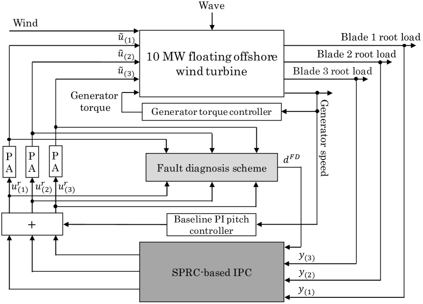
Figure 1: Block diagram of the proposed architecture including FD scheme and SPRC-based IPC, baseline controller and 10MW FOWT. (PA: pitch actuator)

Fig. 1 shows the block diagram of the proposed fault tolerant control architecture, which includes a model-based FD block, the switching SPRC-based IPC, a baseline Collective Pitch Controller (CPC, Jonkman and Buhl 2005) and the 10MW FOWT. Regarding the simulation environment, the aero-hydro-structural dynamic part of the 10MW FOWT is simulated in the widely-used Fatigue, Aerodynamics, Structures, and Turbulence (FAST) numerical package (Jonkman and Buhl, 2005), while the baseline wind turbine control part, SPRC-based IPC and FD scheme are implemented in MathWorks Simulink. In particular, the pitch control utilizes the SPRC-based IPC while the FD scheme uses a model-based approach, both will be introduced in Section 3, for detection and identification of PAS type of faults. It produces a fault decision $d^{\textrm{FD}}\in\{0,\,1,\,2,\,3\}$ where $d^{\textrm{FD}}=0$ indicates no fault, and $d^{\textrm{FD}}=l\neq 0$ indicates the $l$–th pitch actuator is faulty. The decision $d^{\textrm{FD}}$ is fed to the SPRC-based IPC block where it is used to switch the controller parameters to offline-learned values as described in the rest of the paper.

The aero-hydro-structural dynamics of the FOWT can be described by the following nonlinear discrete-time system

$$\begin{cases}x_{k+1}\!\!\!&=A^{0}x_{k}+\rho(x_{k},\tilde{u}_{k})+\eta^{x}(x_{k},\tilde{u}_{k},k)\\ \tilde{u}_{k}\!\!\!&=u_{k}+\beta(k-k_{0})\phi(u_{k},\vartheta)\\ y_{k}\!\!\!&=C^{0}x_{k}+\eta^{y}(x_{k},\tilde{u}_{k},k)\end{cases}\,,$$ (1)

where $k=0,1,\dots$ is the discrete time index and $x\in\mathbb{R}^{n}$, $\tilde{u}\in\mathbb{R}^{q}$, $y\in\mathbb{R}^{q}$ with $q=3$ denote the FOWT state, the control input and the measurement output vectors, respectively. The matrix $A^{0}\in\mathbb{R}^{n\times{n}}$ and the vector field $\rho:\mathbb{R}^{n}\times\mathbb{R}^{q}\mapsto\mathbb{R}^{n}$ describe the nominal linear and nonlinear parts of the FOWT healthy nominal dynamics while $C^{0}\in\mathbb{R}^{l\times{n}}$ is the nominal output matrix. The unavoidable modelling uncertainties and periodic disturbances caused by wind loading as well as measurement noise are characterized by the unknown but bounded functions $\eta^{x}:\mathbb{R}^{n}\times\mathbb{R}^{q}\times\mathbb{R}\mapsto\mathbb{R}^{n}$ and $\eta^{y}:\mathbb{R}^{n}\times\mathbb{R}^{q}\times\mathbb{R}\mapsto\mathbb{R}^{q}$. The output $y$ contains the measurements of the three blades root load.

In order to account for the possible effect of a PAS fault, the term $\tilde{u}$ is used to denote the actual physical value of the three blades pitch angles, while $u$ represents the value that would have been produced by a healthy actuator. The two variables are related by the term $\beta(k-k_{0})\phi(u_{k},\vartheta)$, where $\beta$ is the discrete time unit step, $k_{0}$ is the unknown index of the fault occurrence time and

$$\begin{gathered}\phi_{k}=(-u_{k}+\vartheta)e^{f}\,,\end{gathered}$$ (2)

is the PAS fault function. The unit vector $e^{f}\in\mathbb{R}^{r}$ has a single 1 in its $f$–th position, with $f$ being the index of the stuck actuator while the stuck-at values are contained in $\vartheta\in\mathbb{R}^{r}$. Finally, the nominal healthy angle $u$ is assumed to depend on the reference value $u^{r}$ provided by the pitch control system via a second order transfer function

$$u=\frac{bs+1}{a^{2}s^{2}+bs+1}u^{r}\,,$$

with $a=1/\omega^{ac}$ and $b=2\beta^{ac}/\omega^{ac}$, in which angular frequency $\omega^{ac}=6.28\text{rad/s}$ and damping $\beta^{ac}=0.7$.

3 Fast adaptive fault accommodation

The theoretical framework behind the proposed architecture will be elaborated in detail in this section. The key points are summarized in the following two steps: Step 1: An online model-based FD scheme is developed for FOWTs to detect and isolate PAS faults. Step 2: A SPRC-based IPC is reconfigured to accommodate PAS faults based on the FD results.

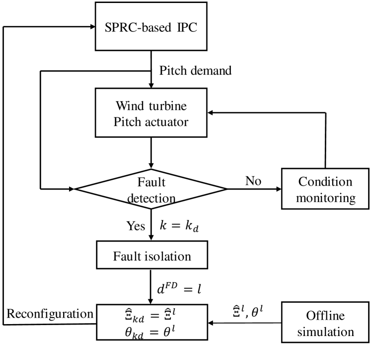
Figure 2: A flowchart showing the main steps and signals involved in the proposed integrated FD and SPRC architecture.

3.1 Model-based fault diagnosis for pitch actuator faults

The online FD scheme in step 1 is now introduced. Following Ferrari et al. (2008), a bank of $N=3$ Fault Detection and Isolation Estimators (FDIEs), one for each actuator, are designed to yield each an output estimate $\hat{u}^{l}_{k}\in\mathbb{R}$ and a residual signal

$$\begin{gathered}r^{l}_{k}\triangleq\tilde{u}_{k,(l)}-\hat{u}^{l}_{k}\,,\end{gathered}$$ (3)

where $\tilde{u}_{k,(l)}$ denotes the $l$–th component of the vector $\tilde{u}_{k}\in\mathbb{R}^{3}$. The healthy hypothesis would be rejected if the absolute value of at least one residual $r^{l}_{k}$ crosses a suitable time-varying threshold $\bar{r}^{l}_{k}$ at detection time $k_{d}$.

Remark 1

For the sake of simplicity, here only one PAS type of fault is considered in each study case. This means that the $l$–th faulty actuator can be isolated and $d^{\textrm{}FD}$ set to $l$ if the $l$–th residual is the only one crossing its corresponding threshold.

The $l$–th FDIE is based on the following discrete-time estimator

$$\begin{cases}\hat{x}^{l}_{k+1}\!\!&=A^{l}\hat{x}^{l}_{k}+B^{l}u^{r}_{k}+L^{l}(\tilde{u}_{k,(l)}-\hat{u}^{l}_{k})\\ \hat{u}^{l}_{k}\!\!&=C^{l}\hat{x}^{l}_{k}+D^{l}u^{r}_{k}\end{cases}\,,$$ (4)

where $\hat{x}^{l}_{k}\in\mathbb{R}^{K}$ and $\hat{u}^{l}_{k}\in\mathbb{R}^{M}$ represent the predicted state vector and output, respectively. $A^{l}$, $B^{l}$, $C^{l}$ and $D^{l}$, are obtained by implementing a state space realization of the $l$–th actuator dynamics (Fontanella et al., 2018). The matrix $L\in\mathbb{R}^{K\times{M}}$ is an estimator gain chosen such that $A^{0,l}\triangleq{A^{l}-L^{l}C^{l}}$ is stable. A time-varying threshold $\bar{r}^{l}_{k}$, guaranteed to bound the healthy $r^{l}_{k}$, is defined as

$$\begin{gathered}\bar{r}^{l}_{k}\triangleq\sum_{h=0}^{k-1}\alpha\delta^{k-1-h}[\bar{\Delta}\rho_{h}+\bar{\eta}^{x}_{h}]+\alpha\delta^{k}\bar{\epsilon}^{x}_{0}+\bar{\eta}^{y}_{k}\end{gathered}\,,$$ (5)

where the two constants $\alpha$ and $\delta$ are calculated as in the paper (Zhang et al. (2001)), such that ${\|C^{l}(A^{0,l})^{k}\|}\leq{\alpha\delta^{k}}\leq{\|C^{l}\|\|A^{0,l}\|^{k}}$. The terms $\bar{\eta}^{x}>\|\eta^{x}\|$ and $\bar{\eta}^{y}>\|\eta^{y}\|$ are known upper bounds on the uncertainties. In addition, $\bar{\epsilon}^{x}_{0}>\|x_{0}-\hat{x}^{l}_{0}\|$ denotes an upper bound on the initial value of the state estimation error. The difference between the real nonlinear dynamics and the value computed by the FDIE is denoted by $\Delta\rho$, with $\bar{\Delta}\rho$ being its upper bound

$$\begin{gathered}\Delta\rho(x_{k},\hat{x},u_{k})\triangleq\rho(x_{k},u_{k})-\rho(\hat{x}_{k},u_{k})\,,\\ \bar{\Delta}\rho(\hat{x}_{k},u_{k})\triangleq\max_{x\in{R^{x}}}(\|\Delta\rho(x,\hat{x},u_{k})\|)\end{gathered}$$ (6)

3.2 Subspace predictive repetitive control

After a PAS type of fault is detected and isolated via the designed FD scheme, the SPRC-based IPC (Navalkar et al., 2014) is reconfigured based on the FD results to accommodate the fault, as summarized in step 2. In detail, the dynamics of the SPRC-based IPC of FOWTs under faulty conditions can be described by the following LTI system affected by unknown periodic disturbances (Houtzager et al., 2013). In prediction form, it is

$$\begin{cases}x_{k+1}\!\!&=\tilde{A}x_{k}+B(u_{k}+\phi_{k})+\tilde{E}d_{k}+Ly_{k}\\ y_{k}\!\!&=Cx_{k}+Fd_{k}+e_{k}\end{cases}\,,$$ (7)

where $d_{k}$ denotes the periodic component of disturbances on the blades, while $e_{k}\in\mathbb{R}^{l}$ is the aperiodic component of the blade loading. In addition, $\tilde{A}\triangleq{A-LC}$ and $\tilde{E}\triangleq{E-LF}$, where matrices $A\in\mathbb{R}^{n\times n}$, $B\in\mathbb{R}^{n\times r}$, $C\in\mathbb{R}^{l\times n}$, $L\in\mathbb{R}^{n\times l}$, $E\in\mathbb{R}^{n\times m}$ and $F\in\mathbb{R}^{l\times m}$ represent state transition, input, output, observer, periodic noise input and periodic noise direct feed-through matrices, respectively. During healthy conditions ($0\leq{k}<{k_{0}}$), it holds $\phi_{k}=0$. The effect of the periodic disturbance on the input-output system could be eliminated by defining a periodic difference operator $\delta$ as,

$$\delta{d}_{k} =d_{k}-d_{k-P}=0,$$

$$\delta{u}_{k} =(u_{k}+\phi_{k})-(u_{k-P}+\phi_{k-P}),$$

$$\delta{y}_{k} =y_{k}-y_{k-P},$$

where $P$ denotes the disturbance period. During the occurrence of a PAS type of fault, $\delta{u}_{k,(f)}$ for the $f$–th blade is 0, since $\phi_{k}=\phi_{k-P}$ accordingly.

Based on the definition of $\delta$, eq. (7) is formulated as

$$\begin{cases}\delta{x}_{k+1}\!\!&=\tilde{A}\delta{x}_{k}+B\delta{u}_{k}+L\delta{y}_{k}\\ \delta{y}_{k}\!\!&=C\delta{x}_{k}+\delta{e}_{k}\end{cases}$$ (8)

Considering a given time window of length $p$ in the past, the following stacked vector can be defined,

$$\delta{U}^{[p]}_{k}=\left[\begin{array}[]{c}u_{k}-u_{k-P}\\ u_{k+1}-u_{k-P+1}\\ \vdots\\ u_{k+p-1}-u_{k+p-P-1}\end{array}\right]\,,$$ (9)

and, similarly, the vector $\delta{Y}^{[p]}_{k}$. If $p$ is large enough such that $\tilde{A}^{j}\approx 0$ $\forall{j}\geq{p}$ (Chiuso (2007)), the future state vector $\delta{x}_{k+p}$ can be approximated based on $\delta{U}^{[p]}_{k}$ and $\delta{Y}^{[p]}_{k}$ as

$$\delta{x}_{k+p}=\left[\begin{array}[]{cc}K^{[p]}_{u}&K^{[p]}_{y}\end{array}\right]\left[\begin{array}[]{c}\delta{U}^{[p]}_{k}\\ \delta{Y}^{[p]}_{k}\\ \end{array}\right]\,,$$ (10)

where $K^{[p]}_{u}$ and $K^{[p]}_{y}$ are defined as,

$$\ K^{[p]}_{u}=\left[\begin{array}[]{cccc}\tilde{A}^{p-1}B&\tilde{A}^{p-2}B&\cdots&B\end{array}\right]\,,$$

$$\ K^{[p]}_{y}=\left[\begin{array}[]{cccc}\tilde{A}^{p-1}L&\tilde{A}^{p-2}L&\cdots&L\end{array}\right]\,.$$

Combining eq. (10) with (8), $\delta\hat{y}_{k}$ can be estimated as

$$\delta{y}_{k+p}=\underbrace{\left[\begin{array}[]{cc}CK^{[p]}_{u}&CK^{[p]}_{y}\end{array}\right]}_{\Xi}\left[\begin{array}[]{c}\delta{U}^{[p]}_{k}\\ \delta{Y}^{[p]}_{k}\\ \end{array}\right]+\delta{e_{k+p}}\,,$$ (11)

where the Markov matrix $\Xi\in\mathbb{R}^{l\times((r+l)\cdot{p})}$ was introduced. In essence, the aim of the identification is to find an online solution of a Recursive Least-Squares (RLS) optimization problem. In order to achieve adaptive tolerant control for the PAS type of fault, the RLS optimization is decoupled for each blade based on the assumption that the $n$–th blade load is independent from the $m$-th, where $n\neq{m}$. Therefore, the subspace identification step for faulty conditions is implemented by the following RLS optimization

$$\hat{\Xi}_{k,(l)}=\text{arg}\min_{\hat{\Xi}_{k}}\sum_{k=0}^{\infty}\left\lVert\delta{y}_{k,(l)}-\lambda\hat{\Xi}_{k,(l)}\left[\begin{array}[]{c}\delta{U}^{[p]}_{k,(l)}\\ \delta{Y}^{[p]}_{k,(l)}\\ \end{array}\right]\right\rVert^{2}_{2}\,,$$ (12)

where $\lambda$ denotes a forgetting factor ($0\ll\lambda\leq{1}$) to attenuate the effect of past data, and adapt to the updated system dynamics online. In this paper, a large value, i.e. $\lambda=0.99999$, was selected to guarantee the robustness of the optimization process (Gustafsson, 2000). $l=1,2,3$ represents the blade number, while $\hat{\Xi}_{k,(l)}$ is the estimate of independent Markov matrix for each blade. As a consequence, the optimization process in eq. (12) is conducted three times at each time instant $k$. Next, the $\hat{\Xi}_{k}$ is synthesized as $\hat{\Xi}_{k}=[\hat{\Xi}_{k,(1)},\hat{\Xi}_{k,(2)},\hat{\Xi}_{k,(3)}]^{T}$. Therefore, the FOWT system dynamics are identified online, taking into consideration the faulty conditions due to the occurrence of PAS. It is noted that the FOWT system should be persistently excited in order to obtain a unique solution of the RLS optimization (Verhaegen and Verdult, 2007). Then, the RLS problem is solved via a QR algorithm, as introduced in Sayed and Kailath (1998). Consequently, the estimates of $\hat{\Xi}_{k}$ are employed to formulate a SPRC law.

The state feedback controller can be formulated with a state-space representation (Navalkar et al., 2014) based on the identified $\hat{\Xi}_{k}$,

$$\underbrace{\left[\begin{array}[]{c}\bar{Y}_{j+1}\\ \delta{\theta}_{j+1}\\ \delta{\bar{Y}}_{j+1}\\ \end{array}\right]}_{\bar{K}_{j+1}}=\underbrace{\left[\begin{array}[]{ccc}I_{l\cdot{P}}&\phi^{+}\widehat{\Gamma^{[P]}K^{[P]}_{u}}\phi&\phi^{+}\widehat{\Gamma^{[P]}K^{[P]}_{y}}\phi\\ 0_{l\cdot{P}}&0_{r\cdot{P}}&0_{l\cdot{P}}\\ 0_{l\cdot{P}}&\phi^{+}\widehat{\Gamma^{[P]}K^{[P]}_{u}}\phi&\phi^{+}\widehat{\Gamma^{[P]}K^{[P]}_{y}}\phi\end{array}\right]}_{\bar{A}_{j}}\\ \underbrace{\left[\begin{array}[]{c}\bar{Y}_{j}\\ \delta{\theta}_{j}\\ \delta{Y}_{j}\end{array}\right]}_{\bar{K}_{j}}+\underbrace{\left[\begin{array}[]{c}\phi^{+}\hat{H}^{[P]}\phi\\ I_{r\cdot{P}}\\ \phi^{+}\hat{H}^{[P]}\phi\end{array}\right]}_{\hat{B}_{j}}\delta{\theta}_{j+1}\,,$$ (13)

where $j=0,1,2,\cdots$ is the rotation count of the rotor. $\hat{H}^{[P]}$ and $\Gamma^{[P]}$ are the same matrices defined in the paper (Navalkar et al. (2014)). The symbol $+$ represents the Moore-Penrose pseudo-inverse. $\theta\in\mathbb{R}^{2r}$ denotes the control inputs projected on the basis function $\phi$, analogously to the study (van de Wijdeven and Bosgra (2010)),

$$U^{[P]}_{k}=\phi\cdot\theta_{j}\,.$$ (14)

It is worth noting that $\theta$ is updated at each $P$. The state transition and input matrices are updated at each discrete time instance $k$. Based on this, the classical optimal state feedback matrix ${K}_{f,j}$ can be synthesised in a Linear Quadratic Regulator (LQR) sense (Hallouzi et al. (2006)). Given the state feedback law, the control signal for the frequency of interest, e.g. 1P, is formulated, as

$$\delta\theta_{j+1}=-K_{f,j}\bar{K}_{j}\,,$$ (15)

Considering that $\delta\theta_{j+1}=\theta_{j+1}-\theta_{j}$, the projected output update law $\theta_{j+1}$ can be calculated as,

$$\theta_{j+1}=\sigma\theta_{j}-\beta{K}_{f,j}\left[\begin{array}[]{c}\bar{Y}_{j}\\ \delta\theta_{j}\\ \delta\bar{Y}_{j}\end{array}\right]\,,$$ (16)

where $\sigma\in[0,1]$ and $\beta\in[0,1]$ are tuning parameters related to the convergence rate of the algorithm. $K_{f,j}$ denotes the optimal state feedback gain during the formulation of the state feedback controller.

If $l$–th faulty actuator is isolated at $k_{d}$ and $d^{FD}=l$, the pre-tuned values of SPRC parameters, i.e. $\theta^{l}$ and $\hat{\Xi}^{l}$, are switched online to initialize the controller as, 1) $\theta_{k_{d}}=\theta^{l}$, 2) $\hat{\Xi}_{k_{d}}=\hat{\Xi}^{l}$. A flow-chart of the proposed integrated FD and SPRC architecture is presented in Fig. 2.

4 Case study

The effectiveness and benefits of the developed fast adaptive fault accommodation architecture is verified in this section, via a case study on the 10MW FOWT (Fig. 1).

4.1 Model configuration

In total, three Load Cases (LCs), which are characterized by a uniform wind profile, are considered in the case study. The mean hub-height wind speed $U_{\text{hub}}$ are 12, 16 and 20 m/s respectively. In addition, one specific PAS type of fault is chosen for each LC, considering a different pitch angle setting $\vartheta_{(3)}$ equaling to 20^∘, 0^∘, 10^∘ respectively for the stuck blade ($f=3$ in all cases). During each LC, totally 1400s are simulated at a fixed discrete time step of $T_{s}=$ 0.01 s, with a fault occurring at $T_{0}=$900 s. The measured signal is pitch angle for each blade, which was affected by a Gaussian white noise measurement with variance of $1.5^{\circ}$.

In order to guarantee persistence of excitation in the nominal healthy and faulty conditions for online subspace identification in the SPRC-based IPC, a filtered pseudo-random binary signal with a maximum amplitude of $3^{\circ}$ is superimposed on top of the collective pitch demand of blades. Based on the excited FOWT system, the Markov matrix is recursively updated by the RLS algorithm and then used for the generation of the SPRC control law.

4.2 Fast adaptive fault accommodation

In order to appreciate the performance of the designed model-based FD scheme, detection results for LC3 are shown in Fig. 3. Before $T_{0}=900$ s, all the residuals are bounded by their corresponding thresholds, thus verifying the robustness of the threshold. After the fault time $T_{0}$, only the pitch angle residual of blade $\#$3 crosses the corresponding threshold, while others are still bounded by their thresholds (see Fig. 3(a-b)), which imply that the PAS fault is successfully detected and isolated. Hence, the correct fault decision $d^{FD}=l=3,l=f$ is obtained and used for reconfiguring the SPRC-based IPC.

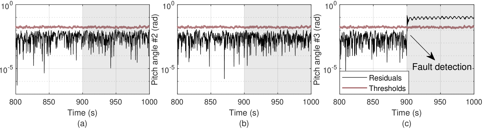
Figure 3: Results of fault diagnosis for PAS type of faults. (a) Pitch angle of blade $\#$1, (b) Pitch angle of blade $\#$2, (c) Pitch angle of blade $\#$3. Time periods of faulty conditions are indicated by a grey background.

Based on the FD results, pre-tuned parameters for the SPRC-based IPC are switched online in order to quickly accommodate the fault. Such new initial values, i.e. $\hat{\Xi}^{l}$ and $\theta^{l}$, have been tuned offline to match the specific faulty blade, thereby reducing the adaptation time. For the offline tuning purpose, two FAST simulations per each possible fault were run to determine $\hat{\Xi}^{l}$ and $\theta^{l}$. In particular the specific PAS type of fault is injected at the beginning of the simulated steady operation of the 10MW FOWT. As a result, time series of $\theta$ in offline simulations, showing the convergence of the SPRC algorithm, are collected. In order to demonstrate the effectiveness and benefits of the proposed architecture, Figs. 4-5 show the comparisons of MOoP and pitch angles between the proposed architecture and other two control logics (i.e. baseline controller and SPRC-based IPC only) in LC3.

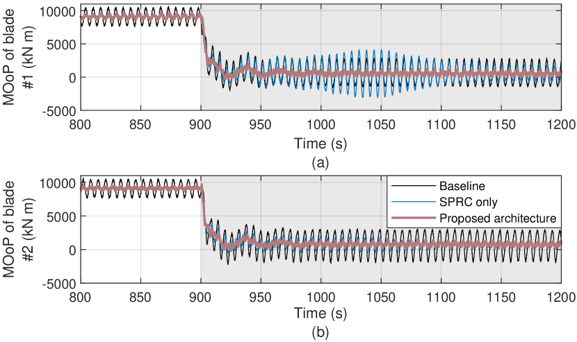
Figure 4: Blade root MOoP. (a) Blade $\#$1, (b) Blade $\#$2. Time periods of faulty conditions are indicated by a grey background. Blade $\#$3 is not shown since it is the faulty blade.

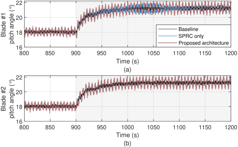
Figure 5: Pitch angles. (a) Blade $\#$1, (b) Blade $\#$2. Time periods of faulty conditions are indicated by a grey background. Blade $\#$3 is not shown since it is the faulty blade.

In nominal healthy conditions, the proposed architecture has the same performance as a non-switched SPRC-based IPC, which is designed to alleviate significantly blade loads in comparison to the turbine baseline controller. After the fault is successfully detected and isolated (Fig. 3), the values of the SPRC parameters are switched to the pre-tuned values in order to quickly accommodate the fault, as shown in Fig. 4 and 5. In the same figures it is possible to notice, as well, that the regular SPRC algorithms may lead to even higher blade loads than the baseline controller during faulty conditions (Fig. 4(a)).

Furthermore, the Power Spectrum Densities (PSDs) of the corresponding MOoP in Fig. 4 within last 200s simulation periods are illustrated in Fig. 6 for investigations.

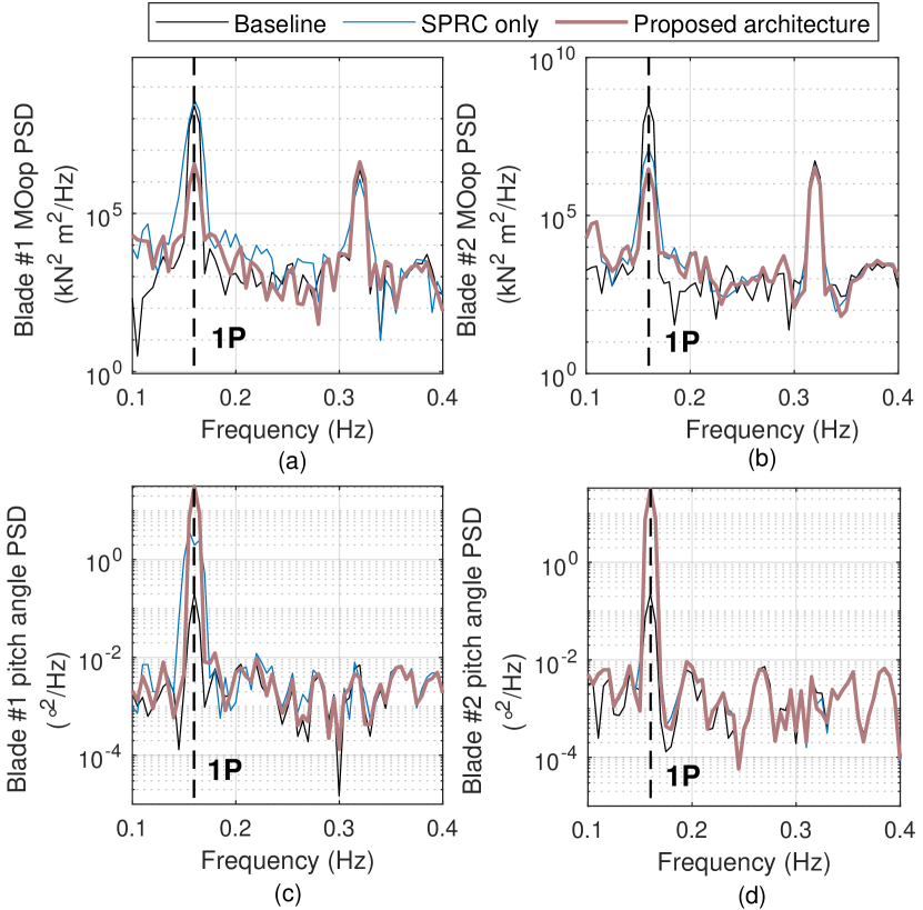
Figure 6: PSD of MOoP and pitch angle. (a) MOoP of blade $\#1$, (b) MOoP of blade $\#2$, (c) Pitch angle of blade $\#1$, (d) Pitch angle of blade $\#2$. Blade $\#3$ is not shown since it is the faulty blade.

It is clear that MOoPs at 1P frequency of blade $\#1$ and $\#2$ are significantly reduced by the pitch angles formulated by the proposed architecture, compared to the baseline controller and SPRC-based IPC only. Particularly, the corresponding $\theta$ in LC3, used to formulate the pitch control demands, are presented in Fig. 7. It is found that the parameter $\theta$, when using the proposed architecture, tends to a value very quickly, which implies a much faster adaptation compared to the SPRC-based IPC only. Similar results are observed in other LCs. In detail, the load reductions compared to the baseline controller are calculated and summarized in Tab. 1. It is clear from this table that the MOoP are significantly reduced by the propose architecture. Particularly, the cumulative MOoP are reduced by the proposed combined FD and SPRC-based IPC by $\sim 66\%$ on average. In comparison, the scheme based on only the SPRC-based IPC attains an average reduction of $\sim 34\%$.

Table 1: Load reduction in faulty conditions in all LCs*.

	LC1 ($\%$)	LC2 ($\%$)	LC3 ($\%$)
SPRC-based IPC only
Blade $\#$1	41.93	60.93	13.89
Blade $\#2$	6.53	55.03	70.12
Cumulative	23.64	56.39	21.65
Proposed architecture
Blade $\#$1	50.53	70.06	80.36
Blade $\#2$	50.54	69.00	83.28
Cumulative	50.23	67.11	80.57

*The number indicates the reduction of the load variance in $\%$.

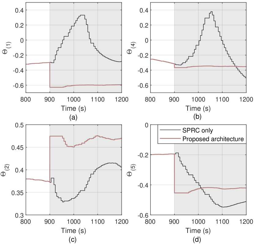
Figure 7: Time series of $\theta$. (a) $\theta_{(1)}$ of blade $\#1$, (b) $\theta_{(4)}$ of blade $\#1$, (c) $\theta_{(2)}$ of blade $\#2$ (d) $\theta_{(5)}$ of blade $\#2$. Time periods of faulty conditions are indicated by a grey background.

5 Concluding remarks

In this paper, a novel architecture is proposed to accommodate the PAS type of faults in a fast adaptive way. In detail, a model-based FD scheme is developed for pitch actuators in FOWTs to detect and isolate PAS type of pitch actuator faults. Based on the fault isolation results, a pre-tuned SPRC-based IPC is switched online to accommodate the detected PAS type of faults, whose initial values of the parameters has been tuned offline to match the specific faulty condition. The effectiveness and benefits of the proposed architecture are illustrated via a case study of a 10MW FOWT in different LCs. Results show that the proposed architecture, integrating the FD scheme and SPRC-based IPC, is able to significantly alleviate the PAS-induced loads. More importantly, the time needed to reduce the PAS-induced loads are significant shortened, which, to some extent, avoids further damage to other components of FOWTs due to the possible improper control demands formulated by the SPRC-based IPC only during the slow adaption time, and thereby allow continued power generation.

References

- Carroll et al. (2016) Carroll, J., McDonald, A., and McMillan, D. (2016). Failure rate, repair time and unscheduled O&M cost analysis of offshore wind turbines. Wind Energy, 19(6), 1107–1119.
- Chiuso (2007) Chiuso, A. (2007). The role of vector autoregressive modeling in predictor-based subspace identification. Automatica, 43(6), 1034 – 1048.
- Ferrari et al. (2008) Ferrari, R.M.G., Parisini, T., and Polycarpou, M.M. (2008). A robust fault detection and isolation scheme for a class of uncertain input-output discrete-time nonlinear systems. In 2008 Am. Control Conf., 2804–2809.
- Fontanella et al. (2018) Fontanella, A., Bayati, I., and Belloli, M. (2018). Linear coupled model for floating wind turbine control. Wind Engineering, 42(2), 115–127.
- Gustafsson (2000) Gustafsson, F. (2000). Adaptive filtering and change detection. Wiley.
- Hallouzi et al. (2006) Hallouzi, R., Verhaegen, M., Babuška, R., and Kanev, S. (2006). Model weight and state estimation for multiple model systems applied to fault detection and identification. IFAC Proceedings Volumes, 39(1), 648 – 653. 14th IFAC Symposium on Identification and System Parameter Estimation.
- Houtzager et al. (2013) Houtzager, I., van Wingerden, J.W., and Verhaegen, M. (2013). Wind turbine load reduction by rejecting the periodic load disturbances. Wind Energy, 16(2), 235–256.
- Jiang et al. (2014) Jiang, Z., Karimirad, M., and Moan, T. (2014). Dynamic response analysis of wind turbines under blade pitch system fault, grid loss, and shutdown events. Wind Energy, 17(9), 1385–1409.
- Jonkman and Buhl (2005) Jonkman, J.M. and Buhl, M.L. (2005). Fast user’s guide. SciTech Connect: FAST User’s Guide.
- Li et al. (2018) Li, D., Li, P., Cai, W., Song, Y., and Chen, H. (2018). Adaptive fault-tolerant control of wind turbines with guaranteed transient performance considering active power control of wind farms. IEEE T. on Ind. Electron., 65(4), 3275–3285.
- Navalkar et al. (2014) Navalkar, S., van Wingerden, J.W., van Solingen, E., Oomen, T., Pasterkamp, E., and van Kuik, G. (2014). Subspace predictive repetitive control to mitigate periodic loads on large scale wind turbines. Mechatronics, 24(8), 916 – 925.
- Ohlenforst et al. (2019) Ohlenforst, K., Sawyer, S., Dutton, A., Backwell, B., Fiestas, R., Joyce, L., Qiao, L., Zhao, F., and Balachandran, N. (2019). Global wind statistics 2018. Report, Global wind energy council.
- Ribrant (2006) Ribrant, J. (2006). Reliability performance and Maintenance—A survey of failure in wind power systems. Thesis, KTH School of Electrical Engineering.
- Sayed and Kailath (1998) Sayed, H. and Kailath, T. (1998). Recursive Least-Squares Adaptive Filters. Press LLC.
- van de Wijdeven and Bosgra (2010) van de Wijdeven, J. and Bosgra, O. (2010). Using basis functions in iterative learning control: analysis and design theory. Int. J. of Control, 83(4), 661–675.
- Verhaegen and Verdult (2007) Verhaegen, M. and Verdult, V. (2007). Filtering and system identification: a least squares approach. Cambridge university press.
- Zhang et al. (2001) Zhang, X., Polycarpou, M., and Parisini, T. (2001). Robust fault isolation for a class of non-linear input-output systems. Int. J. Control, 74(13), 1295–1310.