Specialization in Hierarchical Learning Systems

Abstract

Joining multiple decision-makers together is a powerful way to obtain more sophisticated decision-making systems, but requires to address the questions of division of labor and specialization. We investigate in how far information constraints in hierarchies of experts not only provide a principled method for regularization but also to enforce specialization. In particular, we devise an information-theoretically motivated on-line learning rule that allows partitioning of the problem space into multiple sub-problems that can be solved by the individual experts. We demonstrate two different ways to apply our method: (i) partitioning problems based on individual data samples and (ii) based on sets of data samples representing tasks. Approach (i) equips the system with the ability to solve complex decision-making problems by finding an optimal combination of local expert decision-makers. Approach (ii) leads to decision-makers specialized in solving families of tasks, which equips the system with the ability to solve meta-learning problems. We show the broad applicability of our approach on a range of problems including classification, regression, density estimation, and reinforcement learning problems, both in the standard machine learning setup and in a meta-learning setting.

1 Introduction

Intelligent agents are often conceptualized as decision-makers that learn probabilistic models of their environment and optimize utilities or disutilities like cost or loss functions VonNeumann2007 . In the general case we can think of a utility function as a black-box oracle that provides a numerical score that rates any proposed solution to a supervised, unsupervised or reinforcement learning problem. In context of decision-making, naïvely enumerating all possibilities and searching for an optimal solution is usually prohibitively expensive. Instead, intelligent agents must invest their limited resources in such a way that they achieve an optimal trade-off between expected utility and resource costs in order to enable efficient learning and acting. This trade-off is the central issue in the fields of bounded or computational rationality with repercussions across other disciplines including economics, psychology, neuroscience and artificial intelligence payne1993adaptive ; Simon1955 ; aldrich1999organizations ; manson2006bounded ; gigerenzer2009homo ; damasio2009neuroscience ; Gershman2015 ; Genewein2015 ; Hihn2018 . The information-theoretic approach to bounded rationality is a particular instance of bounded rationality where the resource limitations are modeled by information constraints Edward2014 ; McKelvey1995 ; Tishby2011 ; wolpert2006information ; Ortega2011a ; Ortega2013 ; gottwald2019bounded ; Schach2018 ; lindig2019analyzing closely related to Jaynes’ maximum entropy or minimum relative entropy principle jaynes1996probability .

At the heart of information-theoretic models of bounded rationality lies the information utility trade-off for lossy compression, abstraction and hierarchy formation Genewein2015 . The optimal utility information trade-off leads to an optimal arrangement of decision-makers and encourages the emergence of specialized agents which in turn facilitates an optimal division of labor reducing computational effort Hihn2018 ; Gottwald2019 .

In the context of machine learning, hierarchical inference can also be regarded as an example of bounded rational decision-making with information constraints, where different models correspond to different experts that are bound by their respective priors over parameters and try to optimize the marginal likelihood given data Genewein2015 . The priors that are acquired by the different expert models can be regarded as efficient abstractions that facilitate generalization to novel problems. Hierarchical inference models have been used successfully, for example, to model human behavior when learning with very limited resources from a handful of examples while excelling at adapting quickly jankowski2011meta ; genewein2015structure ; braun2010structure ; kemp2007learning . We can study sample-efficient adaptation to new problems as an instance of “learning to learn” or meta-learning thrun2012learning ; schmidhuber1997shifting ; caruana1997multitask which is an ongoing and active field of research koch2015siamese ; vinyals2016matching ; Finn2017model ; ravi2017optimization ; ortega2019meta ; botvinick2019reinforcement ; yao2019hierarchically . While we can define meta-learning in different ways lemke2015metalearning ; vilalta2002perspective ; giraud2008metalearning ; brazdil2008metalearning ; hutter2019automated , a common denominator is that systems capable of meta-learning happen to learn on two levels, each with a different time scale: slow learning across different tasks (the meta-level), and fast learning to adapt to each task individually. Understanding efficient meta-learning still poses a challenging machine learning problem, as applying pre-trained models to new tasks naïvely usually leads to poor performance, as with each new incoming batch of data the agent has to perform expensive and slow re-learning of its policy.

In this study, we aim to harness the efficient adaptation and the ability of meta-learning of hierarchical inference processes for the learning of decision-making hierarchies formulated in terms of arbitrary utility functions – see Figure 1 and Table 1. The formulation in terms of general utility functions makes this approach applicable to a broad range of machine learning problems that can be formulated as optimization problems, including supervised and unsupervised learning, and reinforcement learning. To this end, we extend our previous work on specialization in hierarchical decision-making systems introduced in Hihn et al.  (2019) hihn2019 to the problem of meta-learning. After introducing information-theoretic constraints for learning and decision-making in Section 2, we explain our hierarchical online learning approach to classification, regression, unsupervised learning and reinforcement learning in Section 3 for the case of within task specialization. We extend our mixture-of-experts learning experiments from Hihn et al.  (2019) hihn2019 for supervised and reinforcement learning in Sections 4.1 and 4.3 and devise a novel application to density estimation in Section 4.2. The extended experiments in the classification and reinforcement learning setting provide new insights into how the number of experts influences the information processing and classification error and how expert policies partition the reinforcement learning problem space amongst themselves. In Sections 5 and 6 we extend the approach from state-based specialization to the case of across task specialization. We show that this task specialization gives rise to a novel meta-learning approach where the meta-learner assigns previously unseen tasks to experts specialized on similar tasks. In order to split the task space and to assign the partitions to experts, we learn to represent tasks through a common latent embedding, which a gating network uses to distribute tasks among the experts–similar to the posterior over models in a hierarchical inference setup. In Section 7, we discuss novel aspects of the current study in the context of previous literature and conclude with a final summary.

2 Information Constraints in Learning and Decision-making

Figure 1: The hierarchical expert model: after observing a world state $x$, the selector samples an expert $m$ according to a selection policy $p(m|x)$ and then the expert samples an action $y$ from the expert’s posterior action policy $p(y|m,x)$. This can be seen as a Gibbs sampling process. Each posterior is the result of a trade-off between maximizing the utility and minimizing the $\operatorname{\text{D}_{\text{KL}}}$ to the respective prior.

2.1 Decision-making with information constraints

Given a utility function $\mathbf{U}(x,y)$ that indicates the desirability of each action $y\in\altmathcal{Y}$ taken in each context $x\in\altmathcal{X}$, a fully rational agent picks action $y^{*}_{x}=\operatorname*{arg\,max}_{y}\mathbf{U}(x,y)$. A bounded rational decision-maker with information constraints Ortega2013 is modeled by an upper bound $B$ on the Kullback-Leibler divergence $\operatorname{\text{D}_{\text{KL}}}(p(y|x)||p(y))=\sum_{y}{p(y|x)\log{\frac{p(y|x)}{p(y)}}}$ between the agent’s prior $p(y)$ and posterior policy $p(y|x)$ to express the limitation on the decision-maker’s information processing resources for reducing uncertainty when optimizing $\mathbf{U}(x,y)$. This results in the following optimization problem:

$$\max_{p(y|x)}\mathbb{E}_{p(y|x)}\left[\mathbf{U}(x,y)\right]-\frac{1}{\beta}\mathbb{E}_{p(x)}\left[\operatorname{\text{D}_{\text{KL}}}(p(y|x)||p(y))\right].$$ (1)

by introducing a Lagrange multiplier $\beta\in\mathbb{R}^{+}$ that is determined by $B$. For $\beta\rightarrow\infty$ we recover the maximum utility solution and for $\beta\rightarrow 0$ the agent can only act according to the prior. In the case of a known state distribution $p(x)$, the optimal prior is given by the marginal $p(y)=\sum_{x}{p(x)p(y|x)}$ and the expected Kullback-Leibler divergence becomes equal to the mutual information $I(X;Y)$.

When aggregating bounded-rational agents into hierarchical decision-making systems that split the action space into soft partitions Genewein2015 , an expert selection policy $p(m|x)$ can be introduced that selects an expert $m$ for a given state $x$ that chooses their action according to a stochastic policy $p(y|x,m)$. Similar to Equation (1), such a hierarchical decision-making system with information constraints can be expressed by the following optimization problem:

$$\max_{p(y|x,m),p(m|x)}\operatorname{\mathbb{E}}[\mathbf{U}(x,y)]-\frac{1}{\beta_{1}}I(X;M)-\frac{1}{\beta_{2}}I(X;Y|M),$$ (2)

where $\beta_{1}$ is the resource parameter for the expert selection stage and $\beta_{2}$ for the experts, and $I(\cdot;\cdot|M)$ denotes the conditional mutual information. The optimal solution is a set of coupled equations

$$\begin{cases}\begin{array}[]{rcl}p(m|x)&=&\frac{1}{Z(x)}p(m)\exp(\beta_{1}\operatorname*{\Delta\text{F}_{\text{par}}}(x,m))\\[2.0pt] p(y|x,m)&=&\frac{1}{Z(x,m)}p(y|m)\exp(\beta_{2}\mathbf{U}(x,y))\\[2.0pt] \end{array}\end{cases}$$ (3)

with the marginals $p(m)=\sum_{x}p(x)p(m|x)$ and $p(y|m)=\sum_{x}p(x|m)p(y|x,m)$, and the free-energy difference $\operatorname*{\Delta\text{F}_{\text{par}}}(x,m)=\operatorname{\mathbb{E}}_{p(y|x,m)}[\mathbf{U}]-\frac{1}{\beta}\operatorname{\text{D}_{\text{KL}}}(p(y|x,m)||p(y|m))$. If we assume $\mathbf{U}(x,y)$ to represent the log-likelihood and $m$ to represent different statistical models with parameters $y$ to explain observables $x$, then Equation (2) describes the problem of hierarchical inference in terms of an optimization problem to produce the posteriors $p(y|x,m)$ and $p(m|x)$.

2.2 Learning with Information Constraints

In learning problems, the true utility $\mathbf{U}(x,y)$ is unknown, instead we are given a function $\mathbf{U}_{D}(x,y)$ after having observed $n$ data samples $D=\{(x_{i},y_{i})\}_{i=1}^{n}$ and we know that $\mathbf{U}_{D}(x,y)\rightarrow\mathbf{U}(x,y)$ for $n\rightarrow\infty$. Assuming that we know $p(x)$, we are looking for the best strategy $p(y|x)$ that optimizes $\mathbf{U}(x,y)$. If we were to treat this as an inference problem, we could index different candidate solutions $p(y|x,\theta)$ with a parameter $\theta$ and place a prior $\pi(\theta)$ over this parameter. From PAC-Bayes analyses it is well-known that the Gibbs distribution $\pi_{D}(\theta)\propto\pi(\theta)\exp\left(\gamma\mathbf{U}_{D}(\theta)\right)$ minimizes the generalization error mcallester2003pac ; mcallester1999pac

$$\mathbb{E}_{\pi_{D}(\theta)}\left[\mathbf{U}(\theta)-\mathbf{U}_{D}(\theta)\right]\leq\sqrt{\frac{\operatorname{\text{D}_{\text{KL}}}(\pi_{D}(\theta)||\pi(\theta))+\log\frac{n}{\delta}}{2(n-1)}}$$

where $U_{n}(\theta)=\frac{1}{n}\sum_{x\in D}\sum_{y}p(y|x,\theta)\mathbf{U}_{D}(x,y)$ and $U(\theta)=\sum_{x,y}p(x)p(y|x,\theta)\mathbf{U}(x,y)$. In a classification problem, for example, we could choose the utility $\mathbf{U}(x,y)=\mathbb{I}_{y=h(x)}$ where $\mathbb{I}$ is the indicator function and $h(x)$ is the mapping from $x$ to the true labels $y_{true}$. Just like the prior $\pi(\theta)$ can be seen to regularize the search for the parameter $\theta$, we can therefore regard the $\operatorname{\text{D}_{\text{KL}}}$ as a principled regularizer in the space of probability distributions over $\theta$. Regularization techniques kukavcka2017regularization ; srivastava2014dropout ; ioffe2015batch are typically introduced to overcome the problem of overfitting (i.e.,  large generalization error), such that we can regard information constraints in $\theta$-space as a particular instance of regularization in the space of hypotheses.

Instead of studying information constraints in hypothesis space governing the update from prior $\pi(\theta)$ to posterior $\pi_{D}(\theta)$, we could also directly study information constraints in the output space governing the update between the prior and posterior predictive distributions $p(y|x)=\sum_{\theta}\pi(\theta)p(y|x,\theta)$ and $p_{D}(y|x)=\sum_{\theta}\pi_{D}(\theta)p(y|x,\theta)$. If the update from $\pi(\theta)$ to $\pi_{D}(\theta)$ is bound by $\operatorname{\text{D}_{\text{KL}}}(\pi_{D}(\theta)||\pi(\theta))\leq C_{1}$, then the update from $p(y|x)$ to $p_{D}(y|x)$ will be bound by $\operatorname{\text{D}_{\text{KL}}}(p_{D}(y|x)||p(y|x))\leq C_{2}$. This suggests that one could try to use the $\operatorname{\text{D}_{\text{KL}}}$ in output space directly as a regularizer. Instead of limiting our search for distributions $p(y|x)$ by imposing a prior in $\theta$-space, we limit our search for $p(y|x)$ directly through a prior $p(y)$ for some suitable $C_{2}$.

Such output regularization techniques have indeed been proposed in the literature. In an unregularized classifier, for example, the probabilities assigned to incorrect class labels would often be pushed close to zero without $\operatorname{\text{D}_{\text{KL}}}$ regularization, such that $p_{\theta}(y|x)$ collapses to a delta function over the correct class label, which is a sign of overfitting szegedy2016rethinking . To avoid this, it has been suggested pereyra2017regularizing to view the probabilities assigned to incorrect labels as knowledge the learner has extracted from the dataset, which can be achieved by encouraging the learner to produce output distributions that balance high entropy and minimal loss:

$$\theta^{*}=\operatorname*{arg\,min}_{\theta}\sum\altmathcal{L}(x,y)-\frac{1}{\beta}H(p_{\theta}(y|x)),$$ (4)

where $x,y$ are training data, $\altmathcal{L}(x,y)$ is a error function and $H(p)=-\sum_{x_{\in}\altmathcal{X}}p(x)\log p(x)$ is the entropy of $p$. This technique introduced by Pereyra et al.  (2017) pereyra2017regularizing has immediate connections to our approach through the following observation: adding the $\operatorname{\text{D}_{\text{KL}}}$ between the agent’s posterior $p_{\theta}(y|x)$ and prior $p(y)$ recovers confidence penalty, if the agent’s prior policy is uniform. A similar idea has also been suggested in the context of using label smoothing as an output regularization technique muller2019does .

In reinforcement learning encouraging the agent to learn policies with high entropy is a widely applied technique known as maximum entropy reinforcement learning (RL) haarnoja2017reinforcement . Maximum entropy RL typically penalizes deviation from a fixed uniformly distributed prior to promote exploration, but in a more general setting we can discourage deviation from an arbitrary prior policy by optimizing for

$$\max_{p}\mathbb{E}_{p}\left[\sum_{t=0}^{\infty}\gamma^{t}\left(r(x_{t},a_{t})-\frac{1}{\beta}\log\frac{p(a_{t}|x_{t})}{p(a)}\right)\right],$$ (5)

where $\beta$ trades off between reward and entropy, such that $\beta\rightarrow\infty$ recovers the standard RL value function and $\beta\rightarrow 0$ recovers the value function under a random policy. While the entropy term is often regarded as a simple method to encourage exploration, we could similarly regard it as an information constraint for regularization to prevent overfitting as in the case of supervised learning.

3 Within Task Specialization in Hierarchical Multi-Agent Policies

Learning Setup and Variables
	Utility	$x$	$m$	$y$
Supervised Learning	neg. MSE / XEnt	data	expert index	label
Unsupervised Learning	log-likelihood	data	model index	parameters
Reinforcement Learning	reward	state	policy index	action

Table 1: Our method exhibits flexibility in that we can address diverse problems by defining different utility functions and expert networks. Note that in the Meta-Learning setup $x$ is a Dataset $D$ defining a task and $m$ is an expert over tasks. To assign datasets we compute feature representations $h(D)$, as we illustrate in Figure 13 in the Appendix.

In the following we introduce the building blocks of our novel gradient based algorithm to learn the components of a hierarchical multi-agent policy with information constraints. In particular, we leverage the hierarchical model introduced earlier to learn a utility driven partitioning of the state and action spaces. We will demonstrate experimentally how limiting the amount of information each agent can process leads to specialization. First we will show how to transform this principle into a general on-line learning algorithm and afterwards we will derive applications to supervised, unsupervised, and reinforcement learning. In Table 1 we summarize the different setups in supervised, unsupervised and reinforcement learning with according utility functions.

The model consists of two stages: an expert selection stage followed by an action selection stage. The first stage learns a soft partitioning of the state space and assigns each partition optimally to the experts according to a parametrized stochastic policy $p_{\theta}(m|x)$ with parameters $\theta$ such that under an information-theoretic constraint we can maximize the free energy $\operatorname*{\Delta\text{F}_{\text{par}}}(x,m)$. We start by rewriting Equation (2) as:

$$\max_{p_{\vartheta}(y|x,m),p_{\theta}(m|x)}\sum_{x,m,y}p(x)p_{\theta}(m|x)p_{\vartheta}(y|x,m)J(x,m,y)$$ (6)

where we define the objective $J(x,m,y)$ as

$$J(x,m,y)=\mathbf{U}(x,y)-\frac{1}{\beta_{1}}\log\frac{p_{\theta}(m|x)}{p(m)}-\frac{1}{\beta_{2}}\log\frac{p_{\vartheta}(y|x,m)}{p(y|m)},$$ (7)

and $\theta,\vartheta$ are the parameters of the selection policy and the expert policies. Note that each expert policy has a distinct set of parameters $\vartheta=\{\vartheta_{m}\}_{m}$, but we drop the $m$ index for readability.

As outlined in Section 2.1, the optimal prior to find an optimal utility information trade-off is the marginal of the posterior policy given by $p(y)=\sum_{x}p(x)p(y|x)$. It would be prohibitive to compute the prior in each step, as it would require marginalizing over large action and state spaces. Instead, we approximate $p(m)$ and $p(y|m)$ by exponential running mean averages of the posterior policies with momentum terms $\lambda_{1}$ and $\lambda_{2}$:

$$p_{t+1}(y|m) = \lambda_{1}p_{t}(y|m)+(1-\lambda_{1})p_{\vartheta}(y|x,m)$$ (8)

$$p_{t+1}(m) = \lambda_{2}p_{t}(m)+(1-\lambda_{2})p_{\theta}(m|x).$$ (9)

3.1 Specialization in Supervised Learning

We set the negative loss as the utility $\operatorname{\mathbf{U}}(y,\hat{y})=-\altmathcal{L}(y,\hat{y})$, where $\hat{y}$ represents the expert’s response (predicted class label, regressed value) and $y$ is the true label. In our implementation we use the cross-entropy loss $\altmathcal{L}(y,\hat{y})=\sum_{i}y_{i}\log\frac{1}{\hat{y}_{i}}=-\sum_{i}y_{i}\log\hat{y}_{i}$ as a performance measure for classification tasks, and for regression the mean squared error $\altmathcal{L}(y,\hat{y})=\sum_{i}||\hat{y}_{i}-y_{i}||^{2}_{2}$ between the prediction $\hat{y}$ and the ground truth values $y$. The selection policy thus optimizes

$$\max_{\theta}\operatorname{\mathbb{E}}_{p_{\theta}(m|x)}\left[\hat{f}(m,x)-\frac{1}{\beta_{1}}\log\frac{p_{\theta}(m|x)}{p(m)}\right],$$ (10)

where $\hat{f}(m,x)\coloneqq\mathbb{E}_{p_{\vartheta}(\hat{y}|m,x)}\big{[}-\altmathcal{L}(\hat{y},y)-\frac{1}{\beta_{2}}\log\frac{p_{\vartheta}(\hat{y}|x,m)}{p(\hat{y}|m)}\big{]}$ is the free energy of expert $m$. Note that this introduces a double expectation, which we can estimate by Monte Carlo sampling. The experts thus simply optimize their free energy objective defined by

$$\max_{\vartheta}\operatorname{\mathbb{E}}_{p_{\vartheta}(\hat{y}|m,x)}\left[-\altmathcal{L}(y,\hat{y})-\frac{1}{\beta_{2}}\log\frac{p_{\vartheta}(\hat{y}|x,m)}{p(\hat{y}|m)}\right].$$ (11)

3.2 Specialization in Unsupervised Learning

Unsupervised learning barlow1989unsupervised deals with learning from data in the face of missing labels, such as clustering xu2008clustering and density estimation silverman2018density algorithms. The density estimation method we propose is similar to RBF Networks schwenker2001three or Gaussian Mixture Models biernacki2000assessing . In the following we will show how our method can handle unsupervised learning, where we interpret each expert as a Normal-Wishart distribution. We model this by learning a distribution $p(\bm{\mu},\bm{\Lambda}|\bm{\omega},\lambda,\bm{W},\nu)$ over means $\bm{\mu}$ and covariance matrices $\bm{\Lambda}$ as Normal-Wishart distributions:

$$p(\bm{\mu},\bm{\Lambda}|\bm{\omega},\lambda,\bm{W},\nu)=\altmathcal{N}\left(\bm{\mu}|\bm{\omega},(\lambda\bm{\Lambda})^{-1}\right)\altmathcal{W}(\bm{\Lambda}|\bm{W},\nu),$$ (12)

where $\altmathcal{W}$ is Wishart a distribution, $\altmathcal{N}$ a Normal distribution, $\bm{\omega}\in\mathbb{R}^{D}$ is the mean of the normal distribution, $\bm{W}\in\mathbb{R}^{D\times D}$ is the scale matrix, $\nu>D-1$ is the degree of freedom, $\lambda>0$ is a scaling factor, and $D$ denotes the dimensionality of the data. Sampling is straightforward: we first sample $\bm{\Lambda}$ from a Wishart distribution with parameters $\mathbf{W}$ and $\nu$. Next we sample $\bm{\mu}$ from a multivariate normal distribution with mean $\bm{\omega}$ and variance $(\lambda\bm{\Lambda})^{-1}$. We assume the data $x$ follows a normal distribution $x\thicksim\altmathcal{N}(\bm{\mu},(\lambda\bm{\Lambda})^{-1})$. The parameters $\nu$, $\lambda$ are hyper-parameters we set beforehand, such that we are interested in finding the parameters $\bm{\mu}^{*}$ and $\bm{W}^{*}$ maximizing the likelihood of the data:

$$\omega^{*},\bm{W}^{*}=\operatorname*{arg\,max}_{\bm{W},\omega}\altmathcal{N}(x|\mu,(\lambda\bm{\Lambda})^{-1})p(\mu,\bm{\Lambda}|\omega,\bm{W},\lambda,\nu)$$ (13)

Thus, in this setting the expert’s task is to find parameters $\omega^{*}$ and $\bm{W}^{*}$ in order to select a tuple $(\bm{\mu},\bm{\Lambda})$ that models the likelihood of the data well. The objective of the selector is to assign data to the experts that not only have a set of parameters that yield high likelihood on the assigned data, but also have low statistical complexity as measured by the $\operatorname{\text{D}_{\text{KL}}}$ between the expert’s posterior and prior distributions. We can now define the free energy difference for each expert as

$$\hat{f}(x,m)=\mathbb{E}_{p_{\vartheta}(\bm{\mu},\bm{\Lambda}|m)}\left[\ell(x|\bm{\mu},(\lambda\bm{\Lambda})^{-1})-\frac{1}{\beta_{2}}\operatorname{\text{D}_{\text{KL}}}(p(\bm{\mu},\bm{\Lambda})||p_{0}(\bm{\omega}_{0},\bm{\Lambda}_{0})\right],$$ (14)

where $p(\bm{\mu},\bm{\Lambda})$ is the expert’s posterior Normal-Wishart distribution over the parameters $\mu$ and $\lambda$ and $p_{0}(\bm{\omega}_{0},\bm{\Lambda}_{0})$ is the expert’s prior, $p$ and $p_{0}$ are the experts posterior and prior distribution and $\ell(x|\bm{\mu},(\lambda\bm{\Lambda})^{-1})$ is the Gaussian log likelihood

$$\ell(x|\bm{\mu},(\lambda\bm{\Lambda})^{-1})=-\frac{1}{2}\log(|(\lambda\bm{\Lambda})^{-1}|)+(x-\bm{\mu})^{T}(\lambda\bm{\Lambda})(x-\bm{\mu})+D\log(2\pi)$$ (15)

of a data point $x$ given the distribution parameters $\bm{\mu},(\lambda\bm{\Lambda})^{-1}$. This serves as the basis for the selector’s task of assigning data to the expert with maximum free energy by optimizing

$$\max_{\theta}\operatorname{\mathbb{E}}_{p_{\theta}(m|x)}\left[\hat{f}(x,m)-\frac{1}{\beta_{1}}\log\frac{p_{\theta}(m|x)}{p(m)}\right].$$ (16)

We can compute the $\operatorname{\text{D}_{\text{KL}}}$ between two Normal-Wishart distributions $p$ and $q$ as

$$\begin{split}\operatorname{\text{D}_{\text{KL}}}\left[p(\bm{\mu},\bm{\Lambda})\|q(\bm{\mu},\bm{\Lambda})\right]=\frac{\lambda_{q}}{2}\left(\bm{\mu}_{q}-\bm{\mu}_{p}\right)^{\top}\nu_{p}\mathbf{W}_{p}\left(\bm{\mu}_{q}-\bm{\mu}_{p}\right)-\\ \frac{\nu_{q}}{2}\log|\bm{W}_{q}^{-1}\bm{W}_{p}|+\frac{\nu_{p}}{2}(\text{tr}(\bm{W}_{q}^{-1}\bm{W}_{p})-D)+C,\end{split}$$ (17)

where $C$ is a term that does not depend on the parameters we optimize, so we can omit it, as we are only interested in relative changes in the $\operatorname{\text{D}_{\text{KL}}}$ caused by changes to $\bm{W}$ and $\bm{\omega}$ (see Appendix B for details on the derivation).

3.3 Specialization in RL Agents

In reinforcement learning we model sequential decision problems by defining a Markov Decision Process (MDP) as a tuple $(\altmathcal{S},\altmathcal{A},P,r)$, where $\altmathcal{S}$ is the set of states, $\altmathcal{A}$ the set of actions, $P:\altmathcal{S}\times\altmathcal{A}\times\altmathcal{S}\rightarrow[0,1]$ is the transition probability, and $r:\altmathcal{S}\times\altmathcal{A}\rightarrow\mathbb{R}$ is a reward function. The aim is to find the parameter $\theta^{*}=\operatorname*{arg\,max}_{\theta}J(p_{\theta})$ of a policy $p_{\theta}$ that maximizes the expected discounted reward $J(p_{\theta})=\mathbb{E}_{p_{\theta}}\left[\sum_{t=0}^{T}\gamma^{t}r(x_{t},a_{t})\right]$. In case of an infinite horizon, we have $T\rightarrow\infty$. We define $r(\tau)=\sum_{t=0}^{T}\gamma^{t}r(x_{t},a_{t})$ as the cumulative reward of trajectory $\tau=\{(x_{t},a_{t})\}_{i=0}^{T}$, where we generate the trajectory according to the policy $p(a_{t}|x_{t})$ and the environmental dynamics $P(x_{t+1}|x_{t},a_{t})$. Reinforcement learning Sutton2018 models assume that an agent interacts with an environment over a number of discrete time steps $t$. At each time step $t$, the agent finds itself in a state $x_{t}$ and selects an action $a_{t}$ according to the policy $p(a_{t}|x_{t})$. In return, the environment transitions to the next state $x_{t+1}$ and generates a scalar reward $r_{t}$. Here, we consider policy gradient methods Sutton2000 which are a popular choice to tackle continuous reinforcement learning problems. The main idea is to directly manipulate the parameters $\theta$ of the policy in order to maximize the objective $J(p_{\theta})$ by taking steps in the direction of the gradient $\nabla_{\theta}J(p_{\theta})$.

In the following we will derive our algorithm for specialization in hierarchical reinforcement learning agents. Note that in the reinforcement learning setup the reward function $r(x,a)$ defines the utility $\mathbf{U}(x,a)$. In maximum entropy RL (see e.g.,  Haarnoja et al.  (2017) haarnoja2017reinforcement ) the regularization penalizes deviation from a fixed uniformly distributed prior, but in a more general setting we can discourage deviation from an arbitrary prior policy by optimizing for:

$$\max_{p}\mathbb{E}_{p}\left[\sum_{t=0}^{T}\gamma^{t}\left(r(x_{t},a_{t})-\frac{1}{\beta}\log\frac{p(a_{t}|x_{t})}{p(a)}\right)\right],$$ (18)

where $\beta$ trades off between reward and entropy, such that $\beta\rightarrow\infty$ recovers the standard RL value function and $\beta\rightarrow 0$ recovers the value function under a random policy.

To optimize the objective (18) we define two separate kinds of value function, $V_{\phi}$ for the selector and one value function $V_{\varphi}$ for each expert. Thus, each expert is an actor-critic with separate actor and critic networks. Similarly, the selector has an actor-critic architecture, where the actor network selects experts and the critic learns to predict the expected free energy of the experts depending on a state variable. The selector’s policy is represented by $p_{\theta}$, while each expert’s policy is represented by a distribution $p_{\vartheta}$.

3.3.1 Value Functions

In standard reinforcement learning the discounted reward is defined as

$$R_{t}=\sum_{l=0}^{T}\gamma^{l}r(x_{t+l},a_{t+l}),$$ (19)

which is usually learned through a parameterized value function $V_{\psi}$ by regressing

$$\psi^{*}=\operatorname*{arg\,min}_{\psi}\frac{1}{|\altmathcal{D}|T}\sum_{\tau\in\altmathcal{D}}\sum_{t=0}^{T}(V_{\psi}(x_{t})-R_{t})^{2}.$$ (20)

Here $\psi$ are some arbitrary parameters of the value representation, $V_{\psi}(x_{t})$ is the predicted value estimate for state $x_{t}$, and $\altmathcal{D}$ is a set of trajectories $\tau$ up to horizon $T$ collected by roll-outs of the policies.

Similar to the standard discounted reward $R_{t}$, we can now define a discounted free energy $F_{t}$ as

$$F_{t}=\sum_{l=0}^{T}\gamma^{l}f(x_{t+l},m_{t+l},a_{t+l}),$$ (21)

where $f(x,m,a)=r(x,a)-\frac{1}{\beta_{2}}\log\frac{p_{\vartheta}(a|x,m)}{p(a|m)}$. Accordingly, we can learn a value function $V_{\varphi}$ for each expert by parameterizing the value function with a neural network and performing regression on $F_{T}$. Similarly, we can define a discounted free energy $\bar{F}_{t}$ for the selector

$$\bar{F}_{t}=\sum_{l=0}^{T}\gamma^{l}\bar{f}(x_{t+l},m_{t+l}),$$ (22)

with $\bar{f}(x,m)=\mathbb{E}_{p_{\vartheta}(a|x,m)}[r(x,a)-\frac{1}{\beta_{2}}\log\frac{p(a|x,m)}{p(a|m)}]$ that is learned through the selector’s value function $V_{\phi}$ by regressing $\bar{F}_{t}$.

3.3.2 Policy Learning

In standard reinforcement learning a common technique to update a parametric policy representation $p_{\omega}(a|x)$ with parameters $\omega$ is to use policy gradients that optimize the cumulative reward

$$J(\omega)=\mathbb{E}\left[p_{\omega}(a|x)V_{\psi}(x)\right]$$ (23)

expected under the critic’s prediction $V_{\psi}(x)$, by following the gradient

$$\nabla_{\omega}J(\omega)=\mathbb{E}\left[\nabla_{\omega}\log p_{\omega}(a|x)V_{\psi}(x)\right].$$ (24)

This policy gradient formulation Sutton2000 is prone to producing high variance gradients. A common technique to reduce the variance is to formulate the updates using the advantage function instead of the reward arulkumaran2017deep . The advantage function $A(a_{t},s_{t})$ is a measure of how well a certain action $a$ performs in a state $x$ compared to the average performance in that state, i.e., $A(a,x)=Q(x,a)-V_{\psi}(x)$. Here, $V(x)$ is the value function and is a measure of how well the agent performs in state $x$, and $Q(x,a)$ is an estimate of the cumulative reward achieved in state $x$ when the agent executes action $a$. Thus, the advantage is an estimate of how advantageous it is to pick $a$ in state $x$ in relation to a baseline performance $V_{\psi}(x)$. Instead of learning the value and the Q function, we can define the advantage function solely based on the critic’s estimate $V_{\psi}(x)$ in the following way

$$A(x_{t},a_{t})=\underbrace{r(x_{t},a_{t})+\gamma V_{\psi}(x_{t+1})}_{\approx Q(x_{t},a_{t})}-V_{\psi}(x_{t}),$$ (25)

giving the following gradient estimates for the policy parameters

$$\omega\leftarrow\omega-\frac{\alpha}{|\altmathcal{D}|}\sum_{\tau\in\altmathcal{D}}\sum_{t=0}^{T}\nabla_{\omega}\log p_{\omega}(a_{t}|x_{t})A(x_{t},a_{t}),$$ (26)

where $\alpha$ is a learning rate and $\altmathcal{D}$ is a set of trajectories $\tau$ produced by the policies.

Similar to the standard policy update based on the advantage function, the expert selection stage can be formulated by optimizing the expected advantage $\mathbb{E}_{p}(a|x,m)\left[A_{m}(x,a)\right]$ for expert $m$ with

$$A_{m}(x_{t},a_{t})=f(x_{t},m,a_{t})+\gamma V_{\varphi}(x_{t+1})-V_{\varphi}(x_{t}).$$

Accordingly, we can define an expected advantage function $\mathbb{E}_{p}(m|x)\left[\bar{A}(x,m)\right]$ for the selector with

$$\bar{A}(x,m)=\mathbb{E}_{p_{\vartheta}(a|x,m)}\left[A_{m}(x,a)\right].$$

We estimate the double expectation by Monte Carlo sampling, where in practice we use a single $(x,m,a)$ tuple for $\hat{f}(x,m)$, which enables us to employ our algorithm in an on-line optimization fashion.

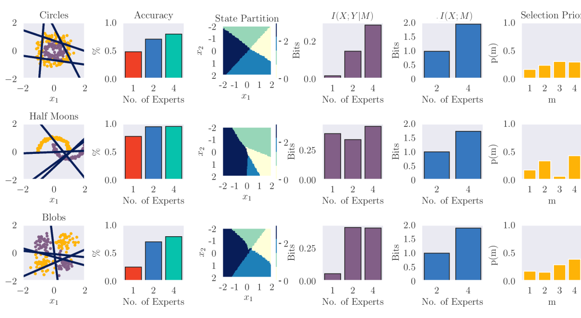
Figure 2: Results for three synthetic classification tasks. Our system successfully enables the linear experts to classify their assigned samples correctly by learning a soft partition of the sample space. As expected the accuracy improves and the information processed by each expert increases, as it specializes on the assigned region. We report all quantities presented in this plot on a 20% hold-out set and averaged over a 10-fold cross-validation scheme.

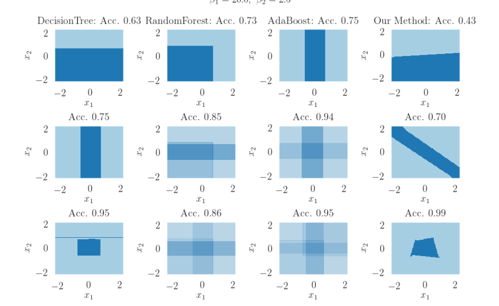
Figure 3: Baseline comparison for the ”Circles” task. Partitioning of the $x_{1},x_{2}$-space is shown for a single decision tree (left column) with depths $1,2,4$, a random forest (middle left column) with $1,2,4$ decision trees of depth $2$, and an Adaboost ensemble (middle right column) of $1,2,4$ decision trees of depth $2$. Our method with $1,2,4$ linear experts is shown in the rightmost column.

4 Experiments and Results: Within Task Specialization

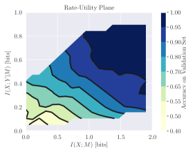
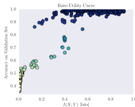
Figure 4: Here we show the influence of the information processing in the expert selection stage and in the expert stage (measured by $I(X;M)$ and $I(X;Y|M)$) on the classification accuracy synthetic dataset “circles” in Figure 2. The grey area is beyond the efficiency frontier of the system. We created this surface by training the system with varying numbers of experts and different settings for $\beta_{1}$ and $\beta_{2}$. We approximate intermediate values by a linear interpolation. The right figure shows the information processing of the whole system given by $I(X;Y)$, which we get by marginalizing over the experts. To obtain a particular information processing rate one must choose both parameters correctly, which can be a bit difficult, as we sweep through these parameters in discrete steps. This causes the bumps and irregularly spaced points on the Rate-Utility grid. Some points are almost impossible to reach even though they are theoretically possible, as the convergence of the learning algorithm may suffer under certain $\beta_{1},\beta_{2}$ configurations.

In the following we will show applications to different learning tasks where the overall complexity of the problem exceeds the processing power of the individual (linear) experts. In particular, we will look at classification, density estimation, and reinforcement learning. See Appendix A for implementation details. In Section 7.2 we discuss how to choose proper values for $\beta_{1}$ and $\beta_{2}$ and their effects on learning.

4.1 Classification with Linear Decision-Makers

When dealing with complex data for classification (or regression) it is often beneficial to combine multiple classifiers (or regressors). In the framework of ensemble learning, for example, multiple classifiers join together to stabilize learning and improve the results Kuncheva2004 , such as Mixture-of-Experts Yuksel2012 and Multiple Classifier systems Bellmann2018 . The method we propose when applied to classification problems falls within this scope of algorithms. The application to regression is an example of local linear regression atkeson1997locally .

We evaluate our method on three synthetic datasets for classification–see Figure 2. Our method is able to partition the problem set into subspaces (third column from the left) and fit a linear decision-maker on each subset, achieving acceptable classification accuracy on synthetic non-linear datasets. The results on the ”Half Moons” dataset show an example where the quality of the classification does not improve with the number of experts, essentially because a satisfactory performance can already be achieved with a single expert. We can see that a single expert is classifying the data reasonably well and adding more experts improves accuracy only marginally, whereas in the remaining two datasets the accuracy increases with the number of experts. Regarding the information processed by each expert $I(X;YvertM)$, a single expert on the ”Half Moons” achieves a competitive score compared to the system with two and four experts, which in turn results in high accuracy. This also manifests in the selection prior $p(m)$ which shows for this dataset a non-uniform division of labor between the experts. In contrast to this, the results on ”Circles” and ”Blobs” show how adding more experts is beneficial if the underlying dataset has a highly non-linear structure. In both settings the information processed by a single expert is close to zero bits and classification accuracy is at chance level. Adding more experts allows for specialization and thus increased processing power $I(X;Y|M)$ which in turn achieves higher classification accuracy.

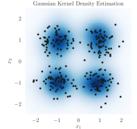
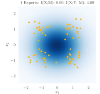
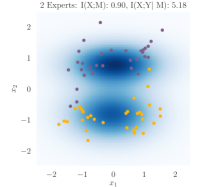
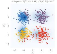
Figure 5: Here we show density estimation results on an artificial dataset. We sampled the data from four bivariate Gaussian distributions ($\mu=\{[-1,-1],[-1,1],[1,1],[1,1]\}$ and $\Sigma=0.15I$) and fit experts on the data. As reference we show the density recovered by gaussian kernel density estimation. Blue indicates high data likelihood. We are able to recover this solution with four experts, but our method allows for additional flexibility by setting the number of experts. As we will show in Section 5, this abstraction gives rise to meta-learning. We set $\beta_{1}=20$ and $\beta_{2}=1.0$.

In Figure 3 we compare the performance of the ”Circles” dataset to different baselines constructed from decision tree learning: a single decision tree with varying depth, multiple decision trees as part of a random forest, and multiple decision trees within Adaboost. In Figure 4 we report how information processing in the selection and the action stage influences classification accuracy. We can see that under a certain threshold the accuracy is random at best and increases with processing power, which is not surprising. Additionally, we can see that a high selection processing power compensates low processing power in the decision-makers up to a certain degree. If the processing power of the experts is too low, adding more experts does not increase the system’s performance indefinitely, as it becomes harder for the selection stage to pick a certain expert. This happens because the experts can only specialize on a small subspace of the task due to their low information-processing capabilities.

4.2 Unsupervised Learning

We report unsupervised learning results in Figure 5, where we show how the system deals with unlabeled data. In this experiment the synthetic dataset contains four clusters and our algorithm is able to perform the clustering as we add more and more experts to partition the state space further. If we provide more experts (in this case 8) than there are clusters (in this case 4), the selector neglects the additional experts and only assigns data to four of them. This indicates that the optimization process aims to find the optimal number of experts in this case.

4.3 Reinforcement Learning with Linear Decision-Makers

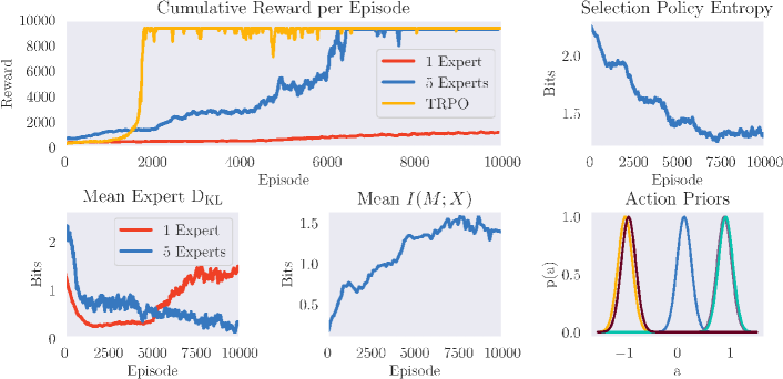
Figure 6: Results for the inverted double pendulum problem. The upper row gives the episodic reward for different system configurations. We show the performance of a system with one linear expert, five linear experts, and compare it to Trust Region Policy Optimization (TRPO) Schulman2015 (discussed further in Section 7.3). We set $\beta_{1}=25$ and $\beta_{2}=2.5$.

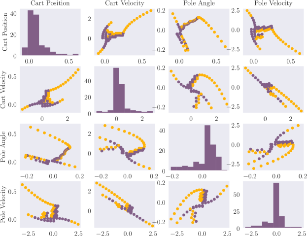
Figure 7: Here we show the pairwise state partition learned by the selection policy on the Cart Pole environment. The task is to keep a pole on a moving cart balanced by applying a control signal $a\in\{-1,+1\}$ which moves the cart to the left or the right. On the diagonal we show the histogram (10 bins) of the state dimension over 100 time steps. Note that the matrix is symmetric.

In the following we will show how our hierarchical system is able to solve a continuous reinforcement learning problem using an optimal arrangement of linear control policies. We evaluate on a task known as Acrobot Sutton1996 , more commonly referred to as the inverted double pendulum. The task is to swing a double-linked pendulum up and keep it balanced as long as possible, where the agent receives a reward of 10 minus a distance penalty between its current state and the goal state. Each episode terminates as soon as the environment reaches a predefined terminal state (hanging downwards) or after 1000 time steps. To balance the pendulum the agent is able to apply a force to the base joint in the range of $a\in[-1,+1]$, thus creating a movement to the left or to the right. This environment poses a non-linear control problem and thus a single linear controller cannot give an optimal solution. We show how using our approach enables a committee of linear experts to efficiently solve this non-linear task. We report the results in Figure 6. We allowed for five experts ($\beta_{2}=2.5$), but our system learns that three experts are sufficient to solve the task. The priors for each expert (lower right Figure, each color represents an expert) center on -1, 0, and 1, which correspond to swinging the double pendulum to the left, no force, and swinging to the right. The remaining two experts overlap accordingly. We can see that the average information processing in the five expert setup decreases, while in the selection it increases to $\log 3$. Both indicate that the system has learned an optimal arrangement of three experts and is thus able to achieve maximum reward and eventually catches up to the performance of a non-linear neural network controller trained with TRPO Schulman2015 that does not have to struggle with the restriction to linear controllers as our algorithm. Our method successfully learned a partitioning of the double-pendulum state space without having any prior information about any of the system dynamics or the state space.

In Figure 7 we show how a model with two linear experts and selector learns to control the cart pole problem. Our method recovers the well known solution in which the pole can be balanced by two linear controllers, where one (dark purple) focuses on keeping the pole upright and the other (dark yellow) on moving the cart such that the other linear controller can take over.

5 Across Task Specialization for Hierarchical Meta-Learning

The methods presented in Section 3 can be easily extended to achieve meta-learning by changing the way the selection mechanism is trained. Instead of assigning individual states that occur within a task, the selector assigns a complete dataset of a task to an expert. To do so, we must find a feature vector $z(d)$ of the dataset $d$. This feature vector must fulfill the following desiderata: 1) invariance against permutation of data in $d$, 2) high representational capacity, 3) efficient computability, and 4) constant dimensionality regardless of sample size $K$. In the following we propose methods to extract such features for image classification, regression, and reinforcement learning problems – see Figure 13. While the experts are trained on the training dataset $D_{\text{meta-train}}$, their performance used to optimize the selection policy is based on the validation dataset $D_{\text{meta-val}}$. The validation dataset contains previously unseen samples that are similar to those in the training set, thus providing a measure for the generalization of each expert. In effect, the selector operates on complete datasets, while the experts operate on single samples.

5.1 Specialization in Meta-Supervised Learning

Algorithm 1 Expert Networks for Supervised Meta-Learning.

1:Input: Data Distribution $p(\altmathcal{D})$, number of samples $K$, batch-size $M$, training episodes $N$ 

2:Hyper-parameters: resource parameters $\beta_{1}$, $\beta_{2}$, learning rates $\eta_{x}$, $\eta_{x}$ for selector and experts 

3:Initialize parameters $\theta,\vartheta$ 

4:for $i$ = 0, 1, 2, …, $N$ do

5:     Sample batch of $M$ datasets $D_{i}\thicksim p(\altmathcal{D})$, each consisting of a training dataset $D_{\text{{meta-train}}}$ and a meta-validation dataset  $D_{\text{{meta-val}}}$ with $2K$ samples each  

6:     for $D\in D_{i}$ do

7:         Find Latent Embedding $z(D_{\text{{meta-train}}})$  

8:         Select expert $m\thicksim p_{\theta}(m|z(D_{\text{{meta-train}}})$  

9:         Compute $\hat{f}(m,D_{\text{meta-val}})$  

10:     end for 

11:     Update selection parameters $\theta$ with $\hat{f}(m,D_{\text{meta-val}})$  

12:     Update Autoencoder with positive samples in $D_{i}$  

13:     Update experts $m$ with assigned $D_{\text{{meta-train}}}$ 

14:end for 

15:return $\theta$, $\vartheta$ 

In a supervised learning task we are usually interested in a dataset consisting of multiple input and output pairs $D=\{(x_{i},y_{i})\}^{N}_{i=1}$ and the learner’s task is to find a function $f(x)$ that maps from input to output, for example through a deep neural network. To do this, we split the dataset into training and test sets and fit a set of parameters $\theta$ on the training data and evaluate on test data using the learned function $f_{\theta}(x)$. In meta-learning, we are instead working with meta-datasets $\altmathcal{D}$, each containing regular datasets split into training and test sets. We thus have different sets for meta-training, meta-validation, and meta-test, i.e.,  $\altmathcal{D}=\{D_{\text{meta-train}},D_{\text{meta-val}},D_{\text{meta-test}}\}$. The goal is to train a learning procedure (the meta-learner) that can take as input one of its training sets $D_{\text{meta-train}}$ and produce a classifier (the learner) that achieves low prediction error on its corresponding test set $D_{\text{meta-test}}$. The meta-learning is then updated using performance measure based on the learner’s performance on $D_{\text{meta-val}}$, compare Algorithm 1. This may not always be the case, but our work (among others, e.g., Finn et al.  (2017) Finn2017model ) follow this paradigm. The rationale being that the meta-learner is trained such that it implicitly optimizes the base learner’s generalization capabilities. The dataset generating distribution $p(\altmathcal{D})$ is unknown to the learner but remains fixed over course of training. The case where $p(\altmathcal{D})$ is changing is study in the field of (meta) continual learning, but is not the focus of this work.

For image classification, we propose to pass the images with positive labels in the dataset through a convolutional autoencoder and use the outputs of the bottleneck layer. Convolutional autoencoders are generative models that learn to reconstruct their inputs by minimizing the Mean-Squared-Error between the input and the reconstructed image (see e.g., Vincent et al.  vincent2008extracting . In this way we get similar embeddings $z(d)$ for similar inputs belonging to the same class. We compute the latent representation for each positive sample in $d$ and pass it through a pooling function $h(z(d))$ to find a single embedding for the complete dataset–see Figure 8 for an overview of our proposed model. We found that max pooling yields the best results, while one could use others, such as mean or min pooling. Yao et al. (2019) yao2019hierarchically propose a similar feature set. For regression, we transform the training data into a feature vector $z(d)$ by binning the points into $N$ bins according to their $x$ value and collecting the $y$ value. If more than one point falls into the same bin we average the $y$ values, thus providing invariance against the order of the data in $D_{\text{meta-train}}$. We use this feature vector to assign each dataset to an expert according to $p_{\theta}(m|h(z(D_{\text{meta-train}})))$, which we abbreviate to $p_{\theta}(m|D_{\text{meta-train}})$.

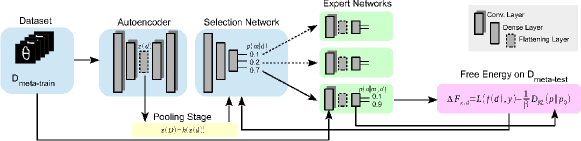
Figure 8: Left: The selector assigns the new input encoding to one of the three experts $\theta_{0}$, $\theta_{1}$ or $\theta_{2}$, depending on the similarity of the input to previous inputs seen by the experts. Right: Our proposed method consists of three main stages. First, we feed the training dataset $D_{\text{train}}$ through a convolutional autoencoder to find a latent representation $z(d_{i})$ for each $d_{i}\in D_{\text{train}}$, which we get by flattening the preceding convolutional layer (“flattening layer”). We apply a pooling function to the resulting set of image embeddings which serves as input to the selection network.

In contrast to the objective defined by Equation (10), the selection policy now selects experts based on their free-energy that is computed over datasets $D_{\text{meta-val}}$ and the selection policy depends on the training datasets $D_{\text{meta-train}}$

$$\max_{\theta}\operatorname{\mathbb{E}}_{p_{\theta}(m|D_{\text{meta-train}})}\left[\hat{f}(m,D_{\text{meta-val}})-\frac{1}{\beta_{1}}\log\frac{p_{\theta}(m|D_{\text{meta-train}})}{p(m)}\right],$$ (27)

where $\hat{f}(m,D_{\text{meta-val}})\coloneqq\mathbb{E}_{p_{\vartheta}(\hat{y}|m,x)}\big{[}-\altmathcal{L}(\hat{y},y)-\frac{1}{\beta_{2}}\log\frac{p_{\vartheta}(\hat{y}|x,m)}{p(\hat{y}|m)}\big{]}$ is the free energy of expert $m$ on dataset $D_{\text{meta-val}}$, $\altmathcal{L}(\hat{y},y)$ is loss function, and $(x,y)\in D_{\text{meta-val}}$. The experts optimize their free energy objective on the training dataset $D_{\text{meta-train}}$ defined by

$$\max_{\vartheta}\operatorname{\mathbb{E}}_{p_{\vartheta}(\hat{y}|m,x)}\left[-\altmathcal{L}(\hat{y},y)-\frac{1}{\beta_{2}}\log\frac{p_{\vartheta}(\hat{y}|x,m)}{p(\hat{y}|m)}\right],$$ (28)

where $(x,y)\in D_{\text{meta-train}}$.

5.2 Specialization in Meta-Reinforcement Learning

Algorithm 2 Expert Networks for Meta-Reinforcement Learning.

1:Input: Environment Distributions $p(T)$ and $p(T^{\prime})$, number of roll-outs $K$, batch-size $M$, training episodes $N$, number of tuples $L$ used for expert selection 

2:Hyper-parameters: resource parameters $\beta_{1}$, $\beta_{2}$, learning rates $\eta_{x}$, $\eta_{x}$ for selector and experts 

3:Initialize parameters $\theta,\vartheta$ 

4:for $i$ = 1, 2, 3, …, $N$ do

5:     Sample batch of $M$ environments $E_{i}^{\text{meta-train}}\thicksim p(T)$ 

6:     for $E\in E_{i}^{\text{meta-train}}$ do

7:         for $k$ = 1, 2, 3, …, $K$ do

8:              Collect $\tau=\{(x_{t},a_{t},r_{t},t)\}_{t=1}^{L}$ tuples by following random expert  

9:              Select expert $m\thicksim p_{\theta}(m|\tau)$ with RNN policy  

10:              Collect trajectory $\tau_{k}=\{(x_{t},a_{t},r_{t},t)\}_{t=L}^{T}$ by following $p_{\vartheta}(a|x,m)$

11:         end for 

12:         Compute $F_{t}=\sum_{l=0}^{T}\gamma^{l}f(x_{t+l},m_{t+l},a_{t+l})$ for trajectories $\tau$ 

13:         where $f(x,m,a)=r_{\text{meta-train}}(x,a)-\frac{1}{\beta_{2}}\log\frac{p_{\vartheta}(a|x,m)}{p(a|m)}$.

14:     end for 

15:     Compute $\bar{F}_{t}=\sum_{l=0}^{T}\gamma^{l}\bar{f}(x_{t+l},m_{t+l})$ with  

16:     $\bar{f}(x,m)=\mathbb{E}_{p_{\vartheta}(a|x,m)}\left[r_{\text{meta-train}}(x,a)-\frac{1}{\beta_{2}}\log\frac{p(a|x,m)}{p(a|m)}\right]$  

17:     Update selection parameters $\theta$ with $\bar{F}$ collected in batch $i$  

18:     Update experts $m$ with roll-outs collected in batch $i$ 

19:end for 

20:return $\theta$, $\vartheta$ 

In meta reinforcement learning we extend the problem to a set of tasks $t_{i}\in T$, where a MDP $t_{i}=(\altmathcal{S},\altmathcal{A},P_{i},r_{i})$ defines each task $t_{i}$. We are now interested in finding a set of policies $\Theta$ that maximizes the average cumulative reward across all tasks in $T$ and generalizes well to new tasks sampled from a different set of tasks $T^{\prime}$.

In this setting we use a dynamic recurrent neural network (RNN) with independent recurrent units li2018independently to classify trajectories and a second RNN to learn the value function (see Appendix A for details). We feed the RNN with $L$ $(s_{t},a_{t},r_{t},s_{t+1})$ tuples to describe the underlying Markov Decision Process describing the task. At $t=0$ we sample the expert according to the learned prior distribution $p(m)$, as there is no other information available until we have collected $L$ samples at which point an expert is selected – see Algorithm 2. Lan et al. (2019) lan2019meta propose a similar feature set. Importantly, the expert policies are trained on the meta-training environments, but evaluated on unseen but similar validation environments. In this setting we define the discounted free energy $\bar{F}_{t}$ for the selector as

$$\bar{F}_{t}=\sum_{l=0}^{T}\gamma^{l}\bar{f}(x_{t+l},m_{t+l}),$$ (29)

with $\bar{f}(x,m)=\mathbb{E}_{p_{\vartheta}(a|x,m)}\left[r_{\text{meta-train}}(x,a)-\frac{1}{\beta_{2}}\log\frac{p(a|x,m)}{p(a|m)}\right]$, where $r_{\text{meta-val}}$ is a reward function defined by a validation environment (see Figure 10 for details).

6 Experimental Results: Across Task Specialization and Meta-Learning

In this section we present our experimental results in the meta-learning domain. To show the flexibility of our method we evaluate on regression, classification and reinforcement learning problems. In regression, we evaluate how our method adapts to changing sine functions, for classification we look at the Omniglot dataset lake2015human . To evaluate on reinforcement learning we introduce a range of versions of the double pendulum task Sutton1996 . We provide all experimental details such as network architectures and hyper-parameters in Appendix B.

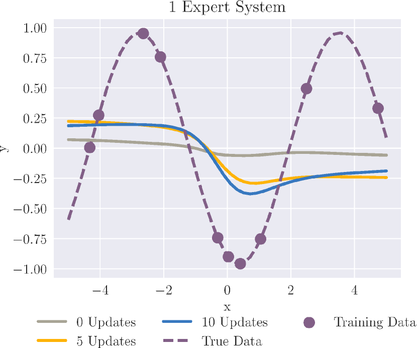
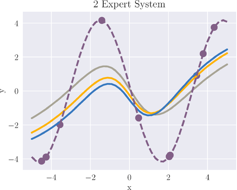
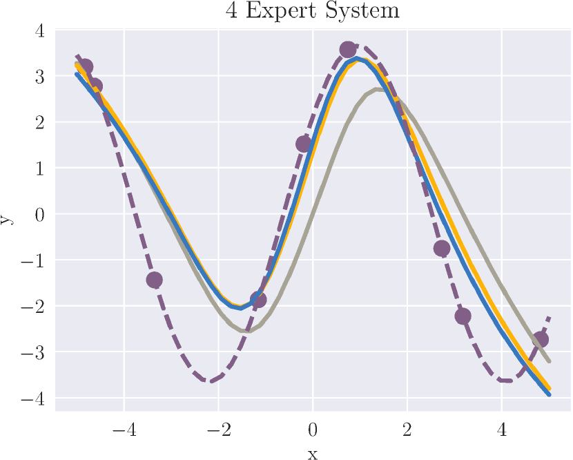
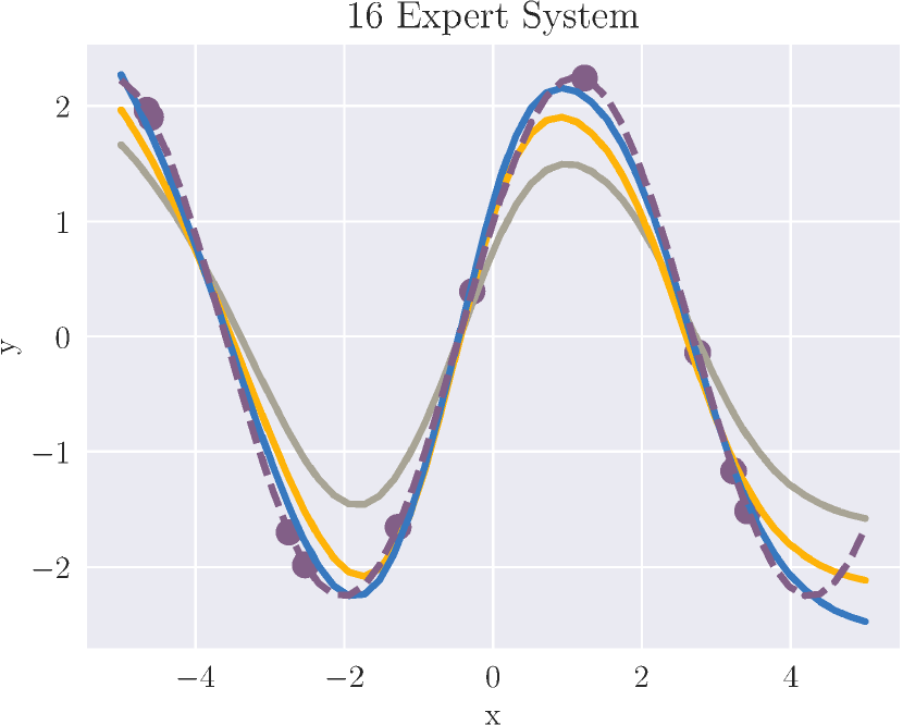
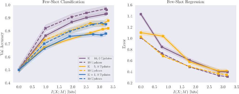
Figure 9: Here show how the system is able to adapt to new problems as the number of experts increases. The single expert system is not able to learn the underlying structure of the sine wave, where the two expert system is already able to capture the periodic structure. Adding more experts improves adaptation further, as the results show. Each expert is a shallow neural network with a single hidden layer and and output layer (see Appendix A for details). In the bottom row we show the rate-utility curve describing the trade-off between information processing and expected utility (transparent area represents one standard deviation), where increasing $I(X;M)$ improves adaptation. To obtain these results we set $\beta_{1}=25$ and $\beta_{2}=1.25$.

6.1 Sinusoid Regression

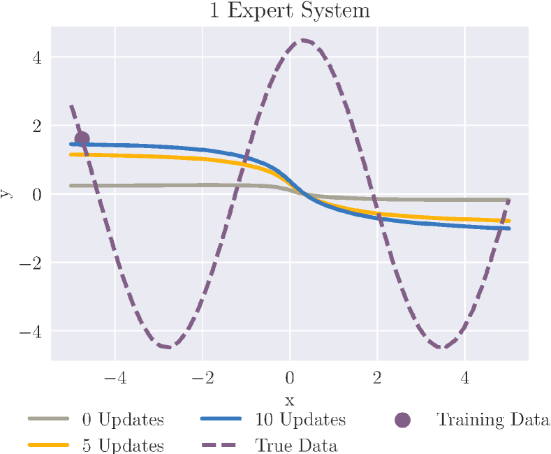
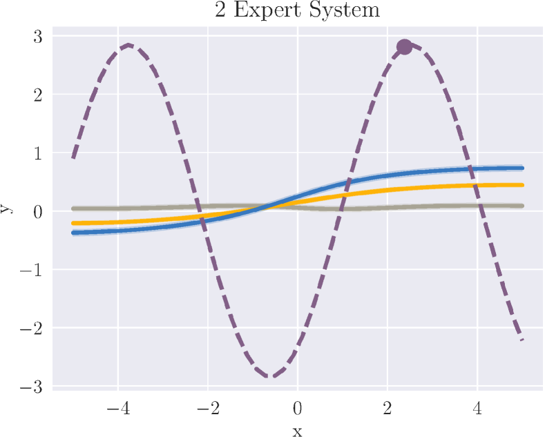
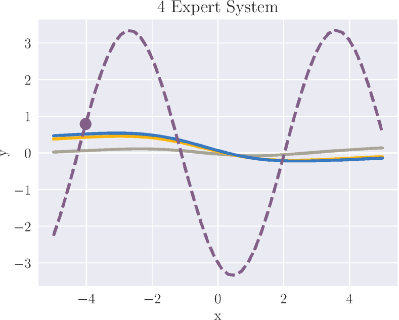
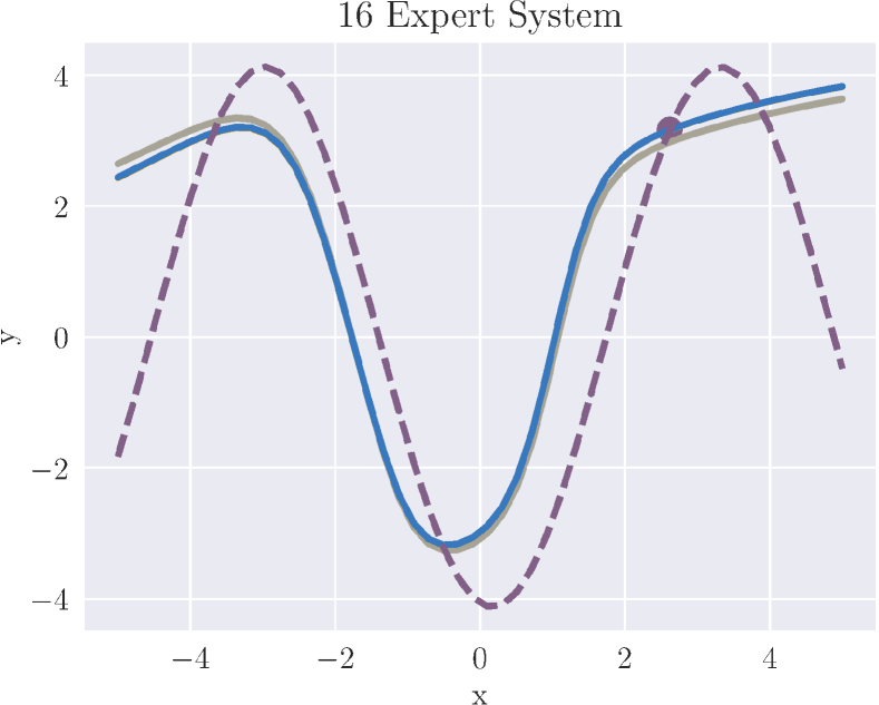
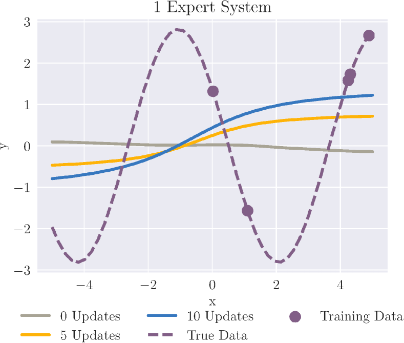
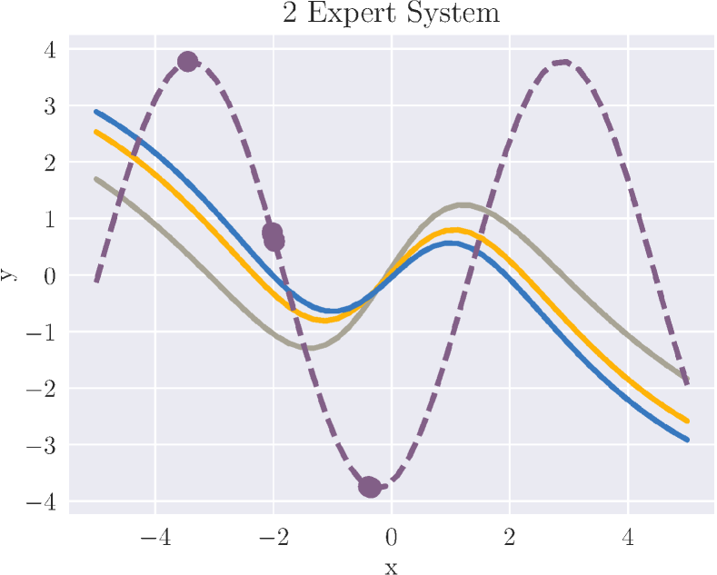
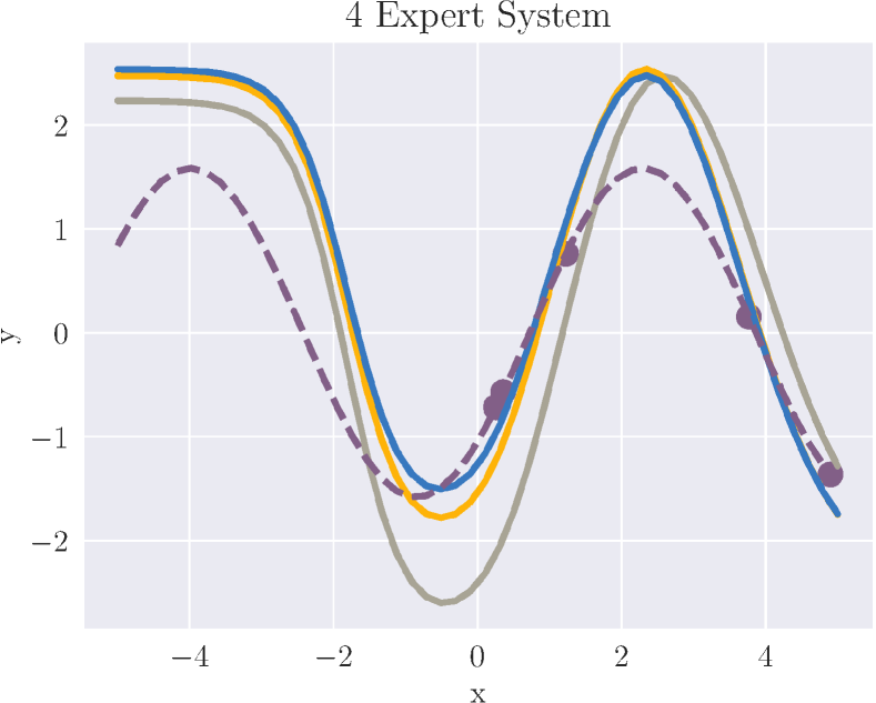
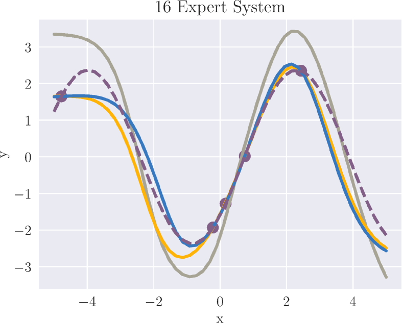
Figure 15: Here show how the system is able to adapt to new problems as the number of experts increases additional results for the $K=1$ (upper row) and $K=5$ (lower row) settings.

We adopt this task from Finn et al.  (2017)  Finn2017model . In this $K$-shot problem, each task consists of learning to predict a function of the form $y=a\cdot\sin(x+b)$, with both $a\in[0.1,5]$ and $b\in[0,2\pi]$ chosen uniformly, and the goal of the learner is to find $y$ given $x$ based on only $K$ pairs of $(x,y)$. Given that the underlying function changes in each iteration it is impossible to solve this problem with a single learner. As a loss function we use Mean-Squared-Error and the dataset embedding is described in Algorithm 1. Each expert is a shallow neural network consisting of a single hidden layer connected to an output layer (see Appendix A for details). Our results show that by combing expert networks, we are able to reduce the generalization error iteratively as we add more experts to our system–see Figure 9 for $K=5$ and $K=10$ settings. In Figure 9 we show how the system is able to capture the underlying problem structure as we add more experts and in Figure 11 we visualize how the selector’s partition of the problem space looks like. In Appendix A, Figure 15 we show additional results and give an overview of our algorithm in Algorithm 1.

6.2 Few-Shot Classification

A special case of meta-learning for classification are $K$-Shot $N$-way tasks, where a training set consists of $K$ labeled examples of each of the $N$ classes ($K\cdot N$ examples per dataset) and a corresponding test set is also provided. In our study, we focus on the following variation of $K$-Shot $N$-Way tasks: $2K$ samples ($K$ positive and $K$ negative examples) define a training dataset which the meta-learner must assign to an expert learner that has a specialized policy to classify the $2K$ samples. To evaluate experts performance we use a meta-validation set consisting of a different set of $2K$ samples. Note that we draw the negative examples from any of the remaining classes.

The Omniglot dataset lake2011one consists of over 1600 characters from 50 alphabets (see Figure 12 for examples ). As each character has merely 20 samples each drawn by a different person, this forms a difficult learning task and is thus often referred to as the ”transposed MNIST” dataset. The Omniglot dataset is a standard meta-learning benchmarking dataset Finn2017model ; vinyals2016matching ; ravi2017optimization .

Omniglot Few-Shot Results
	One Conv. Block Baselines			Methods
	Pre-Training	MAML	Matching Nets	MAML	Matching Nets
K	% Acc	% Acc	% Acc	% Acc	% Acc
1	50.6 ($\pm$ 0.03)	81.2 ($\pm$ 0.03)	52.7 ($\pm$ 0.05)	95.2 ($\pm$ 0.03)	95.0 ($\pm$ 0.01)
5	54.1 ($\pm$ 0.09)	88.0 ($\pm$ 0.01)	55.3 ($\pm$ 0.04)	99.0 ($\pm$ 0.01)	98.7 ($\pm$ 0.01)
10	55.8 ($\pm$ 0.02)	89.2 ($\pm$ 0.01)	60.9 ($\pm$ 0.06)	99.2 ($\pm$ 0.01)	99.4 ($\pm$ 0.01)
Our Method
Number of Experts
	2		4
	% Acc	I(M;X)	% Acc	I(M;X)
1	66.4 ($\pm$ 0.02)	0.99 ($\pm$ 0.01)	75.8 ($\pm$ 0.02)	1.96 ($\pm$ 0.01)
5	67.3 ($\pm$ 0.01)	0.93 ($\pm$ 0.01)	75.5 ($\pm$ 0.01)	1.95 ($\pm$ 0.10)
10	76.2 ($\pm$ 0.04)	0.95 ($\pm$ 0.30)	86.7 ($\pm$ 0.01)	1.90 ($\pm$ 0.03)
	8		16
	% Acc	I(M;X)	% Acc	I(M;X)
1	77.3 ($\pm$ 0.01)	2.5 ($\pm$ 0.02)	82.8 ($\pm$ 0.01)	3.2 ($\pm$ 0.03)
5	78.4 ($\pm$ 0.01)	2.7 ($\pm$ 0.01)	85.2 ($\pm$ 0.01)	3.3 ($\pm$ 0.02)
10	90.1 ($\pm$ 0.01)	2.8 ($\pm$ 0.02)	95.9 ($\pm$ 0.01)	3.1 ($\pm$ 0.02)

Table 2: Classification accuracy after 10 gradient steps on the validation data. Adding experts consistently improves performance, obtaining the best results with an ensemble of 16 experts. Pre-training refers to a single expert system trained on the complete dataset. Our method outperforms the pre-training, Matching Nets, and the MAML baseline (see Appendix A for experimental details), when the network architecture is reduced to a single convolution block. This corresponds to our expert network architecture. Using the suggested architectures by the respective studies, we achieve classification accuracy $\geq 95\%$. In this experiment we set $\beta_{1}=20.0$ and $\beta_{2}=2.5$ for 2 and 4 experts and $\beta_{1}=50.0$ and $\beta_{2}=1.25$ for 8 and 16 experts.

	Task Distribution
Paramater	$T$	$T^{\prime}$
Distance Penalty	[$10^{-3},10^{-1}$]	[$10^{-3},10^{-2}$]
Goal Position	[0.3, 0.4]	[0, 3]
Start Position	[-0.15, 0.15]	[-0.25, 0.25]
Motor Torques	$[0,5]$	$[0,3]$
Motor Actuation	[185, 215]	[175, 225]
Inverted Control	$p=0.5$	$p=0.5$
Gravity	[0.01, 4.9]	[4.9, 9.8]

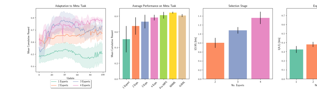
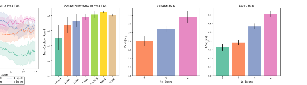
Figure 10: We sample all parameters uniformly from the specified range for each environment, where we use $T$ for training and $T^{\prime}$ for meta evaluation. During training we draw environments from $T$, but evaluate on a different environment also drawn from $T$ to measure generalization. The agent achieves higher reward when adding more experts while the information-processing of the selection and of the expert stage increases, indicating that the added experts specialize successfully. We achieve comparable results to MAML Finn2017model , Proximal Meta-Policy Search (Pro-MPS) rothfuss2018promp , and GrBAL nagabandi2018learning . Shaded areas and error bars represent one standard deviation. See Appendix A for experimental details.

We consider three experimental setups: 1) how does a learner with only a single hidden layer perform when trained naïvely compared to with sophisticated methods such as MAML Finn2017model and Matching Nets vinyals2016matching as a baseline? 2) does the system benefit from adding more experts and if so, at what rate? and 3) how does our method compare to the aforementioned algorithms? Regarding 1) we note that introducing constraints by reducing the representational power of the models does not facilitate specialization is it would by explicit information-processing constraints. In the bottom row of Figure 9 we address question 2). We can interpret this curve as the rate-utility curve showing the trade-off between information processing and expected utility (transparent area represents one standard deviation), where increasing $I(X;M)$ improves adaptation. The improvement gain grows logarithmically, which is consistent with what rate-distortion theory would suggest. In Table 2 we present empirical results addressing question 3).

We train the learner on a subset of the dataset ($\approx 80\%$, $\approx$ 1300 classes) and evaluate on the remaining $\approx 300$ classes, thus investigating the ability to generalize to unseen data. In each round we build the datasets $D_{\text{meta-train}}$ and $D_{\text{meta-test}}$ by selecting a target class $c_{t}$ and sample $K$ positive and $K$ negative samples. To generate negative samples we draw $K$ images randomly out of the remaining $N-1$ classes. We present the selection network with the feature representation of the $K$ positive training samples (see Figure 8), but evaluate the experts’ performance on the $2K$ test samples in $D_{\text{meta-test}}$. We can interpret the free energy of the experts in this setting as a measure of how well the expert is able to generalize to new samples of the target class. Using this optimization scheme, we train the expert networks to become experts in recognizing a subset of classes. We train the experts using the $2K$ samples from the training dataset that the selection network assigned to an expert—see Table 2 for results. We followed the design of Vinyals et al.  vinyals2016matching to design our experts but reduce the number of blocks to one to introduce effects of resource limitation, whereas in the original study the authors used four blocks. The single convolutional block consists of 32 3$\times$3 filters with strided convolutions followed by a batch normalization layer and a ReLu non-linearity. The output is fed into a softmax layer giving a distribution over the classes (see also Appendix A). This reduced representational capacity drives specialization, as the expert can not reliably classify all characters from the training data, but a subset is feasible (see also Figure 12). To evaluate our method we compare different ensemble sizes against three baselines: pre-training, MAML Finn2017model and Matching Networks vinyals2016matching . In the pre-training setting we train a single convolutional neural network on batches drawn from the training data and evaluate on validation data by allowing 10 gradient steps for fine-tuning. Note, that when using the architecture of 4 blocks as suggested in the original paper vinyals2016matching ; Finn2017model , we are able to achieve $\geq$95% accuracy on the test data in both MAML and matching nets, but not on the pre-training setting.

6.3 Meta Reinforcement Learning

In meta reinforcement learning the goal is to find a policy that performs well over a set of tasks. We create a set of RL tasks by extending the “Inverted Double Pendulum problem” Sutton1996 implemented in OpenAI Gym Brockman2016 by allowing a broad range of task parameters. Each time we create a new environment we sample from a specified distribution, where we modify inertia, motor torques, reward function, goal position and invert the control signal – see Table 10 for details. We create one environment per training episode, where during a single training episode parameters remain unchanged. We measure the free energy of an expert on a second task with parameters also drawn from $T$.

To evaluate the agents’ meta-learning capabilities we define a second set of tasks $T^{\prime}$ where the parameter distributions are different, providing new but similar reinforcement learning problems. In each episode we sample $M$ environments from $T$ and update the system batch-wise. After training we evaluate on tasks from $T^{\prime}$, thus testing the agents generalization. We trained the system for 1000 Episodes with 64 tasks from $T$ and evaluate for 100 system updates on tasks from $T^{\prime}$. We report the results in Figure 10, where we can see improving performance as we add more experts, where the mutual information characterizing the selection stage indicates that the selector is able to identify suitable experts for the tasks.

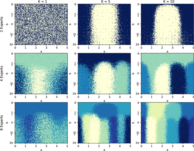
Figure 11: Here we show the soft-partition found by the selection policy for the sine prediction problem $y=a\cdot\sin(x+b)$, where we sample $a,b$ uniformly at each trial and each color represents an expert. To generate these plots we train a system on $K=1,5$ or $10$, sample $a,b$ and $K$ points and feed the dataset to the selection policy. We can see that the selection policy becomes increasingly more precise as we provide more points per dataset (denoted by $K$) to the system.

7 Discussion

7.1 Analyzing the Discovered Meta-Knowledge

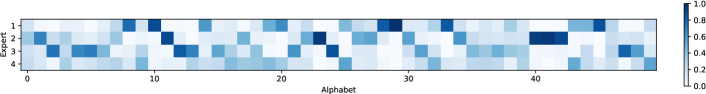
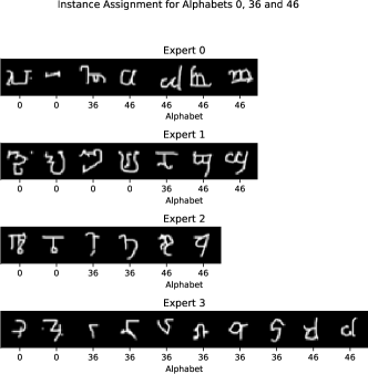
Figure 12: Upper Row: The system learns to assign characters from the same alphabet to the same expert. This happens without any prior information of the concept of alphabets or any other label provided. Lower Row: Here we report selection results on 15 characters sampled from 3 alphabets. To illustrate how the system operates we first show characters from alphabets that the system has difficulties assigning to experts (here alphabets 0, 36, and 46) in the lower left figure. In the lower right figure we show characters from alphabets that the selector assigns with high confidence (10, 11, and 12).

In contrast to monolithic approaches that train a single agent as a black-box we can analyze and interpret the meta-knowledge discovered by our hierarchical method. In the following we will discuss this in the supervised and reinforcement learning setting.

In meta-regression the problem space defined by a set of sine functions $y=a\cdot\sin(x+b)$ is split among the ensemble of expert regressors based on only $K\in\{1,5,10\}$. As expected, the assignment becomes more accurate the more samples we have – see Figure 11 where we report how the selection network partitions the sine task space. The shape of the emerged clusters indicates that the selection is mainly based on the amplitude $a$ of the current sine function, indicating that from an adaptation point-of-view it is more efficient to group sine functions based on amplitude $a$ instead of phase $b$. We can also see that an expert specializes on the low values for $b$ as it covers the upper region of the $a\times b$ space. The selection network splits this region among multiple experts if we increase the set of experts to 8 or more.

We can also analyze the class assignment policy learned by the selector network. The assignment map in Figure 12 suggests that the selector learns to group characters by their alphabet based only on features. The selector’s policy spreads different characters from the same alphabet (e.g., alphabets 0, 36, and 46) across multiple experts while assigning similar characters from different alphabets to the same experts. This specializations gives rise to the meta-learning ability as it is able to adapt expert parameters within only a few gradient steps. We generated this plot by passing images of characters through the system (i.e., computing their latent embedding and assigning them to experts) after training is complete to obtain an overview of the class distribution.

For reinforcement learning we demonstrate this idea by looking at how the selection networks splits the state space into to linearly controllable regions in Figure 7. We can see that one expert receives the states around zero (dark purple) and the other experts sees only states near the boundary (dark yellow). We derive from this that the purple expert specializes on balancing the pole and the yellow expert specializes on moving the cart such that the other expert can easily balance the pole. This is consistent with the fact that a linear policy can balance the pole when it is close to standing upwards.

7.2 Critical issues

A limitation of our method is low sample efficiency in the RL domain. To alleviate this problem one could imagine to combine our system with model-based RL methods which promise to reduce the number of samples the agent needs to see in order to learn efficiently. Another research direction would be to investigate our systems performance in continual adaptation tasks, such as in the work of Yao et al. (2019) yao2019hierarchically . There the agent is continuously exposed to datasets (e.g., additional classes and samples). The restriction to binary meta classification tasks is another limitation of our method, which we leave for feature work.

Another open question remains the tuning of $\beta$ values. As the utility function can in principle be unbounded whereas the information-processing quantities are obviously bounded, the agent may be faced with learning two values that differ greatly in magnitude. This becomes especially challenging in reinforcement learning scenarios, where a value function of varying magnitude has to be learned. This poses a difficult learning problem and there have been several proposals to tackle this. A method dubbed ”Pop-Art” proposed by van Hasselt et al.  (2016) vanHasselt2016learning , where they treat the incoming utility values as a stream of data and normalize the values to given range. In the reinforcement learning setup we also tried cooling schedule for $\beta$, as suggested by Fox et al.  (2015) fox2016taming . In their work the authors propose to change the weight of the entropy penalty in MaxEnt RL as time progresses, thus encouraging exploration in the beginning and penalizing it the more information an agent has gathered. We did not observe any significant performance gains.

The specific value of $\beta$ depends on the scale of the utility function. As the value of $\beta$ strongly influences the outcome of the experiments, it must be chosen with care and comes with the same limitations as any other regularization technique. If it is chosen to small, the regularization term dominates the utility term and the experts are not able to learn anything. On the other hand, if it is set to a large value, the regularization term vanishes, such that no specialization can occur and thus the selector has a hard time assigning data to experts. To remedy this, there are in principle two ways to choose $\beta$: one is to set a information-processing limit for each expert and then (manually or with some optimization technique) tune beta such hat this constraint is satisfied. This has the advantage that this value can be interpreted, e.g., ”the experts can process 1 bit of information, i.e.,  distinguishing two options”. The other way is to run a grid search over a pre-defined range and chose the one that fits best. In this work, we used the second strategy.

7.3 Related Work

Investigating information-theoretic cost functions and constraints in learning systems has recently enjoyed increasing interest in machine learning grau2018soft ; galashov2019information ; grover2019uncertainty ; tschannen2019mutual . The method we propose in this study falls into a wider class of algorithms that aim to deal more efficiently with learning and decision-making problems Daniel2012 ; Neumann2013 ; Martius2013 ; Leibfried2015 ; Grau-Moya2016 ; Peng2017 ; Grau-Moya2017 ; Ghosh2017 ; Hihn2018 ; Schach2018 ; Gottwald2019 ; gottwald2019bounded .

Applying such constraints to methods for reinforcement learning is often motivated by the aim of stabilizing learning and reducing sample complexity. One such approach is Trust Region Policy Optimization (TRPO) introduced by Schulman et al. (2015) Schulman2015 , where a $\operatorname{\text{D}_{\text{KL}}}$ penalty between the old and the new policy is imposed to limit update steps, providing a theoretical guarantee for monotonic policy improvement. In our approach we define this region by $\operatorname{\text{D}_{\text{KL}}}$ between the agent’s posterior and prior policy, thus allowing to learn this region and to adapt it over time. This basic idea has been extend to meta-learning by rothfuss2018promp , which we use to compare our method against in meta-rl experiments. Daniel et al. (2012) follow a similar idea with relative entropy policy search methods Daniel2012 . The algorithm builds on learning a gating policy that can decide which sub-policy to choose. The authors impose a $\operatorname{\text{D}_{\text{KL}}}$ constraint between the data distribution and the next policy to achieve this. Both these approaches smoothen the updates as large steps are discouraged. Our method follows the same principle, but we enforce small updates by discouraging deviation from the agent’s prior and by limiting the representational power (e.g., by linear decision makers).

The hierarchical structure we employ is related to Mixture of Experts (MoE) models. Jacobs et al. (1991) Jacobs1991 introduced MoE as tree structured models for complex classification and regression problems, where the underlying approach is the divide and conquer paradigm. As in our approach, three main building blocks define MoEs: gates, experts, and a probabilistic weighting to combine expert predictions. Learning proceeds by finding a soft partitioning of the input space and assigning partitions to experts performing well on the partition. In this setting, the model response is then a sum of the experts’ outputs, weighted by how confident the gate is in the expert’s opinion. Yuksel et al. (2012) Yuksel2012 provide an extensive overview of recent developments in MoEs. The approach we propose allows learning such models, but also has applications to more general decision-making settings such as reinforcement learning. Ghosh et al. (2017) Ghosh2017 recently applied the divide-and-conquer principle to reinforcement learning. They argue that dividing a central policy into sub-policies improves the learning phase by improving sample efficiency. To evaluate this approach they assume pre-defined partitions on the action and state space on which they train local policies. The information-theoretic constraints during training enforce similarity between the local policies such that a single central policy arises as weighted combination of all local policies. In contrast, in our approach all posterior expert policies remain close to their priors thereby minimizing their informational surprise. This mechanism leads to the emergence of specialized policies. In effect, this enforces the local policies to be as diverse as possible. Crucially, in our method the partitioning is not predefined but a result of the optimization process itself.

Untangling the underlying structure in control systems usually requires a-priori knowledge of the system dynamics, e.g., Abramova2012 ; Randlov2000 ; Yoshimoto2005 . The algorithm proposed by Abramova et al. (2012) Abramova2012 splits the state space of the inverted pendulum into predefined bins to fit a linear control policy to stabilize individually. Then, the authors suggest to control the whole system by learning a selection policy over the given linear controllers. In contrast to this, our approach relies only on the reward signal to learn the selection policy and the linear control policy simultaneously. This fact alone poses a difficult learning problem as both system parts have to adjust to one another on different timescales. Other decentralized approaches (e.g., Allamraju & Chowdhary (2017) allamraju2017communication ) have trained separate decentralized models to fuse them into a single model. In contrast, our method learns sub-policies that act on their own.

Most other methods for meta-learning such as the work of Finn2017model and ravi2017optimization find an initial parametrization of a single learner, such that the agent can adapt quickly to new problems. This initialization represents prior knowledge and can be regarded as an abstraction over related tasks and our method takes this idea one step further by finding a possibly disjunct set of such compressed task properties. Another way of thinking of such abstractions by lossy compression is to go from a task-specific posterior to a task-agnostic prior strategy. By having a set of priors the task specific information is available more locally then with a single prior, as in MAML Finn2017model and the work of ravi2017optimization . In principle, this can help to adapt within fewer iterations. Thus our method can be seen as the general case of such monolithic meta-learning algorithms. Instead of learning similarities within a problem, we can also try to learn similarities between different problems (e.g.,  different classification datasets), as is described in the work of yao2019hierarchically . In this way, the partitioning is governed by different tasks, where our study however focuses on discovering meta-information within the same task family, where the meta-partitioning is determined solely by the optimization process and can thus potentially discover unknown dynamics and relations within a task family.

8 Conclusion

In summary, we introduce and evaluate a promising novel on-line learning paradigm for hierarchical multi-agent systems. The main idea of our approach is an optimal soft partitioning by considering the agents’ information constraints. The partitioning is automatic without relying on any prior information about the underlying problem structure or control dynamics in the case of model free learning. This makes our model abstract and principled. We apply it on a variety of tasks including multi-agent decision-making, mixture-of-expert regression, and divide-and-conquer reinforcement learning. We have extended this idea to a novel information-theoretic approach to meta-learning. In effect, the hierarchical structure equips the system with optimal initializations covering the input space which facilitates quick adaptation to new similar tasks. To build this hierarchical structure, we have proposed feature extraction models for classification, regression and reinforcement learning, that are able to extract task relevant information efficiently, invariant to the order of the inputs. The main strength of our approach is that it follows from simple principles that give rise to a large range of applications. Moreover, we can interpret the system performance by studying the information processing both at the selection stage and at the expert level, as we have shown by analyzing the discovered meta-knowledge. This can help to alleviate the problems inherent to black-box-approaches, for example based on deep neural networks.

Contributions: H.H.  and D.A.B  conceived the project, H.H.  designed and implemented the algorithms and experiments and evaluated the results. Both authors discussed the results and wrote the manuscript. Both authors read and approved the manuscript.

Funding: This research was supported by the European Research Council, grant number ERC-StG-2015-ERC, Project ID: 678082, “BRISC: Bounded Rationality in Sensorimotor Coordination”.

Conflicts of Interest: The authors declare no conflicts of interest.

Appendix A Experimental Details

We implemented all experiments in Tensorflow and ran experiments working with images on a single NVIDIA Tesla V100-SXM2 32GB GPU. We implemented our experiments in TensorFlow [1], Scikit-learn [67] and OpenAI Gym [14].

A Non-Meta-Learning Setting

For classification (Section 4.1) we use a linear predictor as experts, such that the expert’s response is a linear combination of the inputs weighted by some learned parameters $\omega$: $y=\omega^{T}x$ and the selector is a two-layer MLP with 10 units each and tanh non-linearities.

In reinforcement learning (Section 4.3) the selection network is a two layer network with 32 units per layer and tanh non-linearities. Experts are two layer networks with tanh non-linearities that learn log-variance and mean of a Gaussian distribution to predict the control signal. The critic networks have the same architecture but learn directly the value function. As the action space is continuous in the interval [-1,1] we learn $\mu$ and $\log(\sigma)$ of a Gaussian by parameterizing the distribution with a neural network. We sample actions by re-parameterizing the distribution to $p(a)=\mu+\sigma\epsilon$, where $\epsilon\thicksim\altmathcal{N}(0,1)$, so that the distribution is differentiable w.r.t. the network outputs (“re-parametrization trick“ introduced by Kingma and Welling (2013) [44]).

We train all networks using Adam [43] with a learning rate of $3\cdot 10^{-4}$ with Mini-Batch sizes of 32 and sample 1024 data from each task (“Half Moon” etc.) for 10000 episodes. We average the results presented are over 10 random seeds.

B Meta-Learning Setting

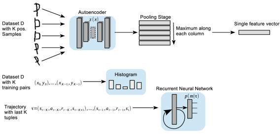
Figure 13: Dataset features in the meta-learning setup. In supervised meta-learning we pass $K$ samples through an convolutional autoencoder producing a $K\times N$ feature matrix, where $N$ is the innermost feature dimension of the autoencoder’s bottleneck layer. To find a single feature vector, we apply a max operator along the columns of the feature matrix. For regression we compute a histogram over the data points. In reinforcement learning, at the start of a trial we sample an expert according to the prior $p(m)$, run the policy for $K$ time steps and use these $K$ $(s,a,r,s^{\prime})$ tuples as input to an recurrent neural network, that acts the selection network to find an expert, which remains active until the environment resets.

The features that we use in the meta-learning setting for the selector in the different learning scenarios are depicted in Figure 13. For regression (Section 6.1) we use a two layer selection network with 16 units each followed by tanh non-linearities. The experts are shallow neural networks with a single hidden layer that learn log-variance and mean of a Gaussian distribution which they use for prediction. We use the “Huber Loss” instead of MSE as it is more robust [7]. We optimize all networks using Adam [43]. We set $\beta_{1}=25$ and $\beta_{2}=1.25$.

For Omniglot (Section 6.2) we followed the design of Vinyals et al.  [90] but reduce the number of blocks to one. We used a single convolutional block consisting of 32 3$\times$3 filters with strided convolutions followed by a batch normalization layer and a ReLu non-linearity. The output is fed into a softmax layer giving a distribution over classes. During training we used a meta-batch size of 16. The convolutional autoencoder is a 3 layer network consisting of 16, 16, and 4 filters each with size 3$\times$3 with strided convolutions followed by a leaky ReLu non-linearity. The layers are mirrored by de-convolotional layers to reconstruct the image. This results in an image embedding with dimensionality 64. The selection network is a two layer network with 32 units, followed by a ReLu non-linearity, a dropout layer [79] per layer and is fed into a softmax normalization to produce a distribution over the experts. For 8 and more experts we add a third layer with 32 units. To improve generalization we add a MaxNorm regularization on the weights. We augment the dataset by rotating each image in 90, 180, and 270 degrees resulting in 80 images per class. We also normalize the images two be in (0,1) range. We evaluate our method by resetting the system to the state after training and allow for 10 gradient updates and report the final accuracy. We train all networks using Adam [43] with a learning rate of $3\cdot 10^{-4}$. In this experiment we set $\beta_{1}=20.0$ and $\beta_{2}=2.5$ for 2 and 4 experts and $\beta_{1}=50.0$ and $\beta_{2}=1.25$ for 8 and 16 experts.

In meta reinforcement learning (Section 6.3) the selector’s actor and critic net are build of RNNs with 200 hidden units each. The critic is trained to minimize the Huber loss between the prediction and the cumulative reward. The experts are two layer networks with 64 units each followed by ReLu non-linearities and used to learn the parameters of a Gaussian distribution. The critics have the same architecture (except for the output dimensionality). The actors learning rate is set to $10^{-4}$ and the critics to $10^{-3}$. We optimize all networks using Adam [43]. We set $\beta_{1}=25.0$ and $\beta_{2}=2.5$.

To evaluate MAML on 2-way $N$-shot omniglot dataset we used a inner learning rate of $\alpha=0.05$ and one inner update step per iteration for all settings. We used a single convolutional block followed by a fully connected layer with 64 units and a ReLU non-linearity. For matching networks we used the same architecture. Note, that we reduce the number of layers to make the tests comparable. Using the suggested architectures [19, 90] we achieve classification accuracy $\geq 95\%$.

Appendix B DKL between two Normal Wishart Distributions

KL divergence from $Q$ to $P$ is defined as $\operatorname{\text{D}_{\text{KL}}}(P\|Q)=\int p(m)\log\frac{p(m)}{q(m)}dx$ and a Normal-Wishart distribution is defined as

$$f(\bm{\mu},\bm{\Lambda}|\bm{\omega},\lambda,\bm{W},\nu)=\altmathcal{N}\left(\bm{\mu}|\bm{\omega},(\lambda\bm{\Lambda})^{-1}\right)\altmathcal{W}(\bm{\Lambda}|\bm{W},\nu),$$

where $\bm{\omega}\in\mathbb{R}^{D},\bm{W}\in\mathbb{R}^{D\times D},\nu>D-1,\lambda>0$ are the parameters of the distribution. We optimize over $\bm{\omega}$ and $\bm{W}$, which makes part of the $\operatorname{\text{D}_{\text{KL}}}$ terms constant. So we have:

$$D_{\mathrm{KL}}\left[\altmathcal{N}_{0}(\bm{\mu})\altmathcal{W}_{0}(\bm{\Lambda})\|\altmathcal{N}_{1}(\bm{\mu})\altmathcal{W}_{1}(\bm{\Lambda})\right] = \int\altmathcal{N}_{0}(\bm{\mu})\altmathcal{W}_{0}(\bm{\Lambda})\log\frac{\altmathcal{N}_{0}(\bm{\mu})\altmathcal{W}_{0}(\bm{\Lambda})}{\altmathcal{N}_{1}(\bm{\mu})\altmathcal{W}_{1}(\bm{\Lambda})}d\bm{\mu}d\bm{\Lambda}$$

Now let

$$p(\bm{\mu},\bm{\Lambda}) = p(\bm{\mu}|\bm{\Lambda})p(\bm{\Lambda})=\altmathcal{N}\left(\bm{\mu}|\bm{\mu}_{0},(\lambda_{0}\bm{\Lambda})^{-1}\right)\altmathcal{W}\left(\bm{\Lambda}|\bm{W}_{0},\nu_{0}\right)$$

$$q(\bm{\mu},\bm{\Lambda}) = q(\bm{\mu}|\bm{\Lambda})q(\bm{\Lambda})=\altmathcal{N}\left(\bm{\mu}|\bm{\mu}_{1},(\lambda_{1}\bm{\Lambda})^{-1}\right)\altmathcal{W}\left(\bm{\Lambda}|\bm{W}_{1},\nu_{1}\right).$$

We can find the $\operatorname{\text{D}_{\text{KL}}}$ as follows:

$$D_{\mathrm{KL}}\left[p(\bm{\mu},\bm{\Lambda})\|q(\bm{\mu},\bm{\Lambda})\right] = \int_{\bm{\mu}}\int_{\bm{\Lambda}}p(\bm{\mu},\bm{\Lambda})\log\frac{p(\bm{\mu},\bm{\Lambda})}{q(\bm{\mu},\bm{\Lambda})}d\bm{\mu}d\bm{\Lambda}$$

$$= \int_{\bm{\mu}}\int_{\bm{\Lambda}}p(\bm{\mu}|\bm{\Lambda})p(\bm{\Lambda})\log\frac{p(\bm{\mu}|\bm{\Lambda})p(\bm{\Lambda})}{q(\bm{\mu}|\bm{\Lambda})q(\bm{\Lambda})}d\bm{\mu}d\bm{\Lambda}$$

$$\stackrel{{\scriptstyle\text{indep.}}}{{=}} \int_{\bm{\mu}}\int_{\bm{\Lambda}}p(\bm{\mu}|\bm{\Lambda})p(\bm{\Lambda})\log\frac{p(\bm{\mu}|\bm{\Lambda})}{q(\bm{\mu}|\bm{\Lambda})}d\bm{\mu}d\bm{\Lambda}$$

$$+\int_{\bm{\mu}}\int_{\bm{\Lambda}}p(\bm{\mu}|\bm{\Lambda})p(\bm{\Lambda})\log\frac{p(\bm{\Lambda})}{q(\bm{\Lambda})}d\bm{\mu}d\bm{\Lambda}$$

$$= \int_{\bm{\Lambda}}p(\bm{\Lambda})\left[\int_{\bm{\mu}}p(\bm{\mu}|\bm{\Lambda})\log\frac{p(\bm{\mu}|\bm{\Lambda})}{q(\bm{\mu}|\bm{\Lambda})}d\bm{\mu}\right]d\bm{\Lambda}$$

$$+\int_{\bm{\Lambda}}p(\bm{\Lambda})\log\frac{p(\bm{\Lambda})}{q(\bm{\Lambda})}d\bm{\Lambda}$$

$$\stackrel{{\scriptstyle\text{def.}}}{{=}} \mathbb{E}_{p(\bm{\Lambda})}\left[\operatorname{\text{D}_{\text{KL}}}\left[p(\bm{\mu}|\bm{\Lambda})\|q(\bm{\mu}|\bm{\Lambda})\right]\right]+\operatorname{\text{D}_{\text{KL}}}\left[p(\bm{\Lambda})\|q(\bm{\Lambda})\right].$$

where $\mathbb{E}_{p(\bm{\Lambda})}[X]=\nu\bm{W}$ and $\operatorname{\text{D}_{\text{KL}}}$ between two Normal Distributions $p(\bm{\mu}|\bm{\Lambda})$ and $q(\bm{\mu}|\bm{\Lambda})$ is

$$\operatorname{\text{D}_{\text{KL}}}\left[p(\bm{\mu}|\bm{\Lambda})\|q(\bm{\mu}|\bm{\Lambda})\right] = \frac{1}{2}\bigg{[}\mathrm{tr}\left((\lambda_{q}\bm{\Lambda})(\lambda_{p}\bm{\Lambda})^{-1}\right)+\left(\bm{\mu}_{q}-\bm{\mu}_{p}\right)^{\top}(\lambda_{q}\bm{\Lambda})\left(\bm{\mu}_{q}-\bm{\mu}_{p}\right)$$

$$-D+\log\frac{\|\lambda_{p}\bm{\Lambda}\|}{\|\lambda_{q}\bm{\Lambda}\|}\bigg{]}$$

$$= \frac{1}{2}\left[D\frac{\lambda_{q}}{\lambda_{p}}+\left(\bm{\mu}_{q}-\bm{\mu}_{p}\right)^{\top}\lambda_{q}\bm{\Lambda}\left(\bm{\mu}_{q}-\bm{\mu}_{p}\right)-D+D\log\frac{\lambda_{q}}{\lambda_{p}}\right],$$

so we have

$$\mathbb{E}_{p(\bm{\Lambda})}\left[D_{\mathrm{KL}}\left[p(\bm{\mu}|\bm{\Lambda})\|q(\bm{\mu}|\bm{\Lambda})\right]\right] = \frac{\lambda_{q}}{2}\left(\bm{\mu}_{q}-\bm{\mu}_{p}\right)^{\top}\nu_{p}\mathbf{W}_{p}\left(\bm{\mu}_{q}-\bm{\mu}_{p}\right)$$

$$+\underbrace{\frac{D}{2}\left(\frac{\lambda_{q}}{\lambda_{p}}-\log\frac{\lambda_{q}}{\lambda_{p}}-1\right)}_{\text{constant term}}.$$

The $\operatorname{\text{D}_{\text{KL}}}$ between two Wishart Distributions $p(\bm{\Lambda})$ and $q(\bm{\Lambda})$ is

$$D_{KL}[p(\bm{\Lambda})$$

$$vertq(\bm{\Lambda})] = H(p(\bm{\Lambda}),q(\bm{\Lambda}))-H(p(\bm{\Lambda}))$$

$$= -\frac{\nu_{q}}{2}\log|\bm{W}_{q}^{-1}\bm{W}_{p}|+\frac{\nu_{p}}{2}(\text{tr}(\bm{W}_{q}^{-1}\bm{W}_{p})-D)$$

$$+\underbrace{\log\frac{\Gamma_{D}\left(\frac{\nu_{q}}{2}\right)}{\Gamma_{D}\left(\frac{\nu_{p}}{2}\right)}+\tfrac{\nu_{p}-\nu_{q}}{2}\psi_{D}\left(\frac{\nu_{p}}{2}\right)}_{\text{constant term}}$$

where $\Gamma_{D}(m)$ is the multivariate Gamma distribution and $\psi_{D}(m)$ is the derivative of the log of the multivariate Gamma distribution, each parameterized by the dimensionality of $\bm{\mu}$ and $\bm{W}$ denoted by $D$. As we keep $\nu$ and $\lambda$ fixed, we can use an estimate, which is only off by constant factor $C$:

$$\begin{split}\operatorname{\text{D}_{\text{KL}}}\left[p(\bm{\mu},\bm{\Lambda})\|q(\bm{\mu},\bm{\Lambda})\right]=\frac{\lambda_{q}}{2}\left(\bm{\mu}_{q}-\bm{\mu}_{p}\right)^{\top}\nu_{p}\mathbf{W}_{p}\left(\bm{\mu}_{q}-\bm{\mu}_{p}\right)-\\ \frac{\nu_{q}}{2}\log|\bm{W}_{q}^{-1}\bm{W}_{p}|+\frac{\nu_{p}}{2}(\text{tr}(\bm{W}_{q}^{-1}\bm{W}_{p})-D)+C\end{split}$$ (30)

where $C=\frac{D}{2}\left(\frac{\lambda_{q}}{\lambda_{p}}-\log\frac{\lambda_{q}}{\lambda_{p}}-1\right)+\log\frac{\Gamma_{D}\left(\frac{\nu_{q}}{2}\right)}{\Gamma_{D}\left(\frac{\nu_{p}}{2}\right)}+\tfrac{\nu_{p}-\nu_{q}}{2}\psi_{D}\left(\frac{\nu_{p}}{2}\right)$

Appendix C Additional Results

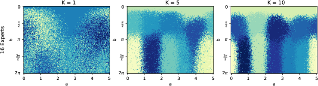
Figure 14: Here we show the soft-partition found by the selection policy for the sine prediction problem $y=a\cdot\sin(x+b)$ for 16 experts, where we sample $a,b$ uniformly at each trial and each color represents an expert.

References

- [1] Martín Abadi, Paul Barham, Jianmin Chen, Zhifeng Chen, Andy Davis, Jeffrey Dean, Matthieu Devin, Sanjay Ghemawat, Geoffrey Irving, Michael Isard, et al. Tensorflow: A system for large-scale machine learning. In 12th USENIX Symposium on Operating Systems Design and Implementation (OSDI 16), pages 265–283, 2016.
- [2] Ekaterina Abramova, Luke Dickens, Daniel Kuhn, and Aldo Faisal. Hierarchical, heterogeneous control of non-linear dynamical systems using reinforcement learning. In European Workshop On Reinforcement Learning at ICML, 2012.
- [3] Howard Aldrich. Organizations evolving. Sage, 1999.
- [4] Rakshit Allamraju and Girish Chowdhary. Communication efficient decentralized gaussian process fusion for multi-uas path planning. In Proceedings of the 2017 American Control Conference (ACC), pages 4442–4447. IEEE, 2017.
- [5] Kai Arulkumaran, Marc Peter Deisenroth, Miles Brundage, and Anil Anthony Bharath. Deep reinforcement learning: A brief survey. IEEE Signal Processing Magazine, 34(6):26–38, 2017.
- [6] Christopher G Atkeson, Andrew W Moore, and Stefan Schaal. Locally weighted learning for control. In Lazy learning, pages 75–113. Springer, 1997.
- [7] S Balasundaram and Yogendra Meena. Robust support vector regression in primal with asymmetric huber loss. Neural Processing Letters, 49(3):1399–1431, 2019.
- [8] Horace B Barlow. Unsupervised learning. Neural computation, 1(3):295–311, 1989.
- [9] Peter Bellmann, Patrick Thiam, and Friedhelm Schwenker. Multi-classifier-systems: Architectures, algorithms and applications. In Computational Intelligence for Pattern Recognition, pages 83–113. Springer, 2018.
- [10] Christophe Biernacki, Gilles Celeux, and Gérard Govaert. Assessing a mixture model for clustering with the integrated completed likelihood. IEEE transactions on pattern analysis and machine intelligence, 22(7):719–725, 2000.
- [11] Mathew Botvinick, Sam Ritter, Jane X Wang, Zeb Kurth-Nelson, Charles Blundell, and Demis Hassabis. Reinforcement learning, fast and slow. Trends in cognitive sciences, 2019.
- [12] Daniel A Braun, Carsten Mehring, and Daniel M Wolpert. Structure learning in action. Behavioural brain research, 206(2):157–165, 2010.
- [13] Pavel Brazdil, Christophe Giraud Carrier, Carlos Soares, and Ricardo Vilalta. Metalearning: Applications to data mining. Springer Science & Business Media, 2008.
- [14] Greg Brockman, Vicki Cheung, Ludwig Pettersson, Jonas Schneider, John Schulman, Jie Tang, and Wojciech Zaremba. Openai gym. arXiv preprint arXiv:1606.01540, 2016.
- [15] Rich Caruana. Multitask learning. Machine learning, 28(1):41–75, 1997.
- [16] Antonio Damasio. Neuroscience and the emergence of neuroeconomics. In Neuroeconomics, pages 207–213. Elsevier, 2009.
- [17] Christian Daniel, Gerhard Neumann, and Jan Peters. Hierarchical relative entropy policy search. In Artificial Intelligence and Statistics, pages 273–281, 2012.
- [18] Vul Edward, Goodman Noah, Griffiths Thomas L., and Tenenbaum Joshua B. One and done? optimal decisions from very few samples. Cognitive Science, 38(4):599–637, 2014.
- [19] Chelsea Finn, Pieter Abbeel, and Sergey Levine. Model-agnostic meta-learning for fast adaptation of deep networks. In Proceedings of the 34th International Conference on Machine Learning-Volume 70, pages 1126–1135. JMLR. org, 2017.
- [20] Roy Fox, Ari Pakman, and Naftali Tishby. Taming the noise in reinforcement learning via soft updates. In Proceedings of the Thirty-Second Conference on Uncertainty in Artificial Intelligence, pages 202–211, 2016.
- [21] Alexandre Galashov, Siddhant M Jayakumar, Leonard Hasenclever, Dhruva Tirumala, Jonathan Schwarz, Guillaume Desjardins, Wojciech M Czarnecki, Yee Whye Teh, Razvan Pascanu, and Nicolas Heess. Information asymmetry in kl-regularized rl. In Proceedings of the International Conference on Representation Learning, 2019.
- [22] Tim Genewein, Eduard Hez, Zeynab Razzaghpanah, and Daniel A Braun. Structure learning in bayesian sensorimotor integration. PLoS Comput Biol, 11(8):e1004369, 2015.
- [23] Tim Genewein, Felix Leibfried, Jordi Grau-Moya, and Daniel Alexander Braun. Bounded rationality, abstraction, and hierarchical decision-making: An information-theoretic optimality principle. Frontiers in Robotics and AI, 2:27, 2015.
- [24] Samuel J Gershman, Eric J Horvitz, and Joshua B Tenenbaum. Computational rationality: A converging paradigm for intelligence in brains, minds, and machines. Science, 349(6245):273–278, 2015.
- [25] Dibya Ghosh, Avi Singh, Aravind Rajeswaran, Vikash Kumar, and Sergey Levine. Divide-and-conquer reinforcement learning. In Proceedings of the International Conference on Representation Learning, 2018.
- [26] Gerd Gigerenzer and Henry Brighton. Homo heuristicus: Why biased minds make better inferences. Topics in cognitive science, 1(1):107–143, 2009.
- [27] Christophe Giraud-Carrier. Metalearning-a tutorial. In Tutorial at the 7th international conference on machine learning and applications (ICMLA), San Diego, California, USA, 2008.
- [28] Sebastian Gottwald and Daniel A. Braun. Bounded rational decision-making from elementary computations that reduce uncertainty. Entropy, 21(4), 2019.
- [29] Sebastian Gottwald and Daniel A Braun. Systems of bounded rational agents with information-theoretic constraints. Neural computation, 31(2):440–476, 2019.
- [30] Jordi Grau-Moya, Matthias Krüger, and Daniel A Braun. Non-equilibrium relations for bounded rational decision-making in changing environments. Entropy, 20(1):1, 2017.
- [31] Jordi Grau-Moya, Felix Leibfried, Tim Genewein, and Daniel A Braun. Planning with information-processing constraints and model uncertainty in markov decision processes. In Proceeedings of the Joint European Conference on Machine Learning and Knowledge Discovery in Databases, pages 475–491. Springer, 2016.
- [32] Jordi Grau-Moya, Felix Leibfried, and Peter Vrancx. Soft q-learning with mutual-information regularization. In Proceedings of the International Conference on Learning Representations, 2019.
- [33] Aditya Grover and Stefano Ermon. Uncertainty autoencoders: Learning compressed representations via variational information maximization. In Proceedings of the The 22nd International Conference on Artificial Intelligence and Statistics, pages 2514–2524, 2019.
- [34] Tuomas Haarnoja, Haoran Tang, Pieter Abbeel, and Sergey Levine. Reinforcement learning with deep energy-based policies. In Proceedings of the 34th International Conference on Machine Learning-Volume 70, pages 1352–1361. JMLR. org, 2017.
- [35] Heinke Hihn, Sebastian Gottwald, and Daniel A Braun. Bounded rational decision-making with adaptive neural network priors. In IAPR Workshop on Artificial Neural Networks in Pattern Recognition, pages 213–225. Springer, 2018.
- [36] Heinke Hihn, Sebastian Gottwald, and Daniel A Braun. An information-theoretic on-line learning principle for specialization in hierarchical decision-making systems. In Proceedings of the 2019 IEEE Conference on Decision-Making and Control (CDC), 2019.
- [37] Frank Hutter, Lars Kotthoff, and Joaquin Vanschoren. Automated Machine Learning. Springer.
- [38] Sergey Ioffe and Christian Szegedy. Batch normalization: Accelerating deep network training by reducing internal covariate shift. arXiv preprint arXiv:1502.03167, 2015.
- [39] Robert A Jacobs, Michael I Jordan, Steven J Nowlan, and Geoffrey E Hinton. Adaptive mixtures of local experts. Neural computation, 3(1):79–87, 1991.
- [40] Norbert Jankowski, Wlodzislaw Duch, and Krzysztof Grkabczewski. Meta-learning in computational intelligence, volume 358. Springer Science & Business Media, 2011.
- [41] Edwin T Jaynes. Probability theory: the logic of science. Washington University St. Louis, MO, 1996.
- [42] Charles Kemp, Amy Perfors, and Joshua B Tenenbaum. Learning overhypotheses with hierarchical bayesian models. Developmental science, 10(3):307–321, 2007.
- [43] Diederik P Kingma and Jimmy Ba. Adam: A method for stochastic optimization. In Proceedings of the International Conference on Representation Learning, 2014.
- [44] Diederik P Kingma and Max Welling. Auto-encoding variational bayes. In Proceedings of the International Conference on Representation Learning, 2013.
- [45] Gregory Koch, Richard Zemel, and Ruslan Salakhutdinov. Siamese neural networks for one-shot image recognition. In ICML deep learning workshop, volume 2, 2015.
- [46] Jan Kukačka, Vladimir Golkov, and Daniel Cremers. Regularization for deep learning: A taxonomy. arXiv preprint arXiv:1710.10686, 2017.
- [47] Ludmila I Kuncheva. Combining pattern classifiers: methods and algorithms. John Wiley & Sons, 2004.
- [48] Brenden Lake, Ruslan Salakhutdinov, Jason Gross, and Joshua Tenenbaum. One shot learning of simple visual concepts. In Proceedings of the Annual Meeting of the Cognitive Science Society, volume 33, 2011.
- [49] Brenden M Lake, Ruslan Salakhutdinov, and Joshua B Tenenbaum. Human-level concept learning through probabilistic program induction. Science, 350(6266):1332–1338, 2015.
- [50] Lin Lan, Zhenguo Li, Xiaohong Guan, and Pinghui Wang. Meta reinforcement learning with task embedding and shared policy. In Proceedings of the International Joint Conference on Artificial Intelligence, 2019.
- [51] Felix Leibfried and Daniel A Braun. A reward-maximizing spiking neuron as a bounded rational decision maker. Neural computation, 27(8):1686–1720, 2015.
- [52] Christiane Lemke, Marcin Budka, and Bogdan Gabrys. Metalearning: a survey of trends and technologies. Artificial intelligence review, 44(1):117–130, 2015.
- [53] Shuai Li, Wanqing Li, Chris Cook, Ce Zhu, and Yanbo Gao. Independently recurrent neural network (indrnn): Building a longer and deeper rnn. In Proceedings of the IEEE conference on computer vision and pattern recognition, pages 5457–5466, 2018.
- [54] Cecilia Lindig-Leon, Sebastian Gottwald, and Daniel Alexander Braun. Analyzing abstraction and hierarchical decision-making in absolute identification by information-theoretic bounded rationality. Frontiers in Neuroscience, 13:1230, 2019.
- [55] Steven M Manson. Bounded rationality in agent-based models: experiments with evolutionary programs. International Journal of Geographical Information Science, 20(9):991–1012, 2006.
- [56] Georg Martius, Ralf Der, and Nihat Ay. Information driven self-organization of complex robotic behaviors. PloS one, 8(5):e63400, 2013.
- [57] David A McAllester. Pac-bayesian model averaging. In Proceedings of the twelfth annual conference on Computational learning theory, pages 164–170, 1999.
- [58] David A McAllester. Pac-bayesian stochastic model selection. Machine Learning, 51(1):5–21, 2003.
- [59] Richard D. McKelvey and Thomas R. Palfrey. Quantal response equilibria for normal form games. Games and Economic Behavior, 10(1):6 – 38, 1995.
- [60] Rafael Müller, Simon Kornblith, and Geoffrey E Hinton. When does label smoothing help? In Advances in Neural Information Processing Systems, pages 4694–4703, 2019.
- [61] Anusha Nagabandi, Ignasi Clavera, Simin Liu, Ronald S Fearing, Pieter Abbeel, Sergey Levine, and Chelsea Finn. Learning to adapt in dynamic, real-world environments through meta-reinforcement learning. In International Conference on Learning Representations, 2018.
- [62] Gerhard Neumann, Christian Daniel, Andras Kupcsik, Marc Deisenroth, and Jan Peters. Information-theoretic motor skill learning. In Proceedings of the AAAI Workshop on Intelligent Robotic Systems, 2013.
- [63] Pedro Ortega and Daniel Braun. Information, utility and bounded rationality. Lecture Notes in Artificial Intelligence, 6830:269–274, 2011.
- [64] Pedro A. Ortega and Daniel A. Braun. Thermodynamics as a theory of decision-making with information-processing costs. Proceedings of the Royal Society of London A: Mathematical, Physical and Engineering Sciences, 469(2153), 2013.
- [65] Pedro A Ortega, Jane X Wang, Mark Rowland, Tim Genewein, Zeb Kurth-Nelson, Razvan Pascanu, Nicolas Heess, Joel Veness, Alex Pritzel, Pablo Sprechmann, et al. Meta-learning of sequential strategies. arXiv preprint arXiv:1905.03030, 2019.
- [66] John W Payne, John William Payne, James R Bettman, and Eric J Johnson. The adaptive decision maker. Cambridge university press, 1993.
- [67] F. Pedregosa, G. Varoquaux, A. Gramfort, V. Michel, B. Thirion, O. Grisel, M. Blondel, P. Prettenhofer, R. Weiss, V. Dubourg, J. Vanderplas, A. Passos, D. Cournapeau, M. Brucher, M. Perrot, and E. Duchesnay. Scikit-learn: Machine learning in Python. Journal of Machine Learning Research, 12:2825–2830, 2011.
- [68] Zhen Peng, Tim Genewein, Felix Leibfried, and Daniel A Braun. An information-theoretic on-line update principle for perception-action coupling. In Proceedings of the 2017 IEEE/RSJ International Conference on Intelligent Robots and Systems (IROS), pages 789–796. IEEE, 2017.
- [69] Gabriel Pereyra, George Tucker, Jan Chorowski, Łukasz Kaiser, and Geoffrey Hinton. Regularizing neural networks by penalizing confident output distributions. In Proceedings of the International Conference on Learning Representations (ICLR), 2017.
- [70] Jette Randløv, Andrew G Barto, and Michael T Rosenstein. Combining reinforcement learning with a local control algorithm. In Proceedings of the International Conference on Machine Learning, 2000.
- [71] Sachin Ravi and Hugo Larochelle. Optimization as a model for few-shot learning. In Proceedings of the International Conference on Learning Representations, 2017.
- [72] Jonas Rothfuss, Dennis Lee, Ignasi Clavera, Tamim Asfour, and Pieter Abbeel. Promp: Proximal meta-policy search. In International Conference on Learning Representations, 2018.
- [73] Sonja Schach, Sebastian Gottwald, and Daniel A Braun. Quantifying motor task performance by bounded rational decision theory. Frontiers in neuroscience, 12, 2018.
- [74] Jürgen Schmidhuber, Jieyu Zhao, and Marco Wiering. Shifting inductive bias with success-story algorithm, adaptive levin search, and incremental self-improvement. Machine Learning, 28(1):105–130, 1997.
- [75] John Schulman, Sergey Levine, Pieter Abbeel, Michael Jordan, and Philipp Moritz. Trust region policy optimization. In Proceedings of the International Conference on Machine Learning, pages 1889–1897, 2015.
- [76] Friedhelm Schwenker, Hans A Kestler, and Günther Palm. Three learning phases for radial-basis-function networks. Neural networks, 14(4-5):439–458, 2001.
- [77] Bernard W Silverman. Density estimation for statistics and data analysis. Routledge, 2018.
- [78] Herbert A. Simon. A behavioral model of rational choice. The Quarterly Journal of Economics, 69(1):99–118, 1955.
- [79] Nitish Srivastava, Geoffrey Hinton, Alex Krizhevsky, Ilya Sutskever, and Ruslan Salakhutdinov. Dropout: a simple way to prevent neural networks from overfitting. The journal of machine learning research, 15(1):1929–1958, 2014.
- [80] Richard S Sutton. Generalization in reinforcement learning: Successful examples using sparse coarse coding. In Advances in neural information processing systems, pages 1038–1044, 1996.
- [81] Richard S Sutton and Andrew G Barto. Reinforcement learning: An introduction. MIT press, 2018.
- [82] Richard S Sutton, David A McAllester, Satinder P Singh, and Yishay Mansour. Policy gradient methods for reinforcement learning with function approximation. In Advances in neural information processing systems, pages 1057–1063, 2000.
- [83] C Szegedy, V Vanhoucke, S Ioffe, J Shlens, and Z Wojna. Rethinking the inception architecture for computer vision. In 2016 IEEE Conference on Computer Vision and Pattern Recognition (CVPR), pages 2818–2826, 2016.
- [84] Sebastian Thrun and Lorien Pratt. Learning to learn. Springer Science & Business Media, 2012.
- [85] Naftali Tishby and Daniel Polani. Information theory of decisions and actions. In Perception-Action Cycle: Models, Architectures, and Hardware. Springer, 2011.
- [86] Michael Tschannen, Josip Djolonga, Paul K Rubenstein, Sylvain Gelly, and Mario Lucic. On mutual information maximization for representation learning. In Proceedings of the International Conference on Representation Learning, 2020.
- [87] Hado P van Hasselt, Arthur Guez, Matteo Hessel, Volodymyr Mnih, and David Silver. Learning values across many orders of magnitude. In Advances in Neural Information Processing Systems, pages 4287–4295, 2016.
- [88] Ricardo Vilalta and Youssef Drissi. A perspective view and survey of meta-learning. Artificial intelligence review, 18(2):77–95, 2002.
- [89] Pascal Vincent, Hugo Larochelle, Yoshua Bengio, and Pierre-Antoine Manzagol. Extracting and composing robust features with denoising autoencoders. In Proceedings of the Proceedings of the 25th international conference on Machine learning, pages 1096–1103. ACM, 2008.
- [90] Oriol Vinyals, Charles Blundell, Timothy Lillicrap, Daan Wierstra, et al. Matching networks for one shot learning. In Advances in neural information processing systems, pages 3630–3638, 2016.
- [91] John Von Neumann and Oskar Morgenstern. Theory of games and economic behavior (commemorative edition). Princeton university press, 2007.
- [92] David H Wolpert. Information theory – the bridge connecting bounded rational game theory and statistical physics. In Complex Engineered Systems, pages 262–290. Springer, 2006.
- [93] Rui Xu and Don Wunsch. Clustering, volume 10. John Wiley & Sons, 2008.
- [94] Huaxiu Yao, Ying Wei, Junzhou Huang, and Zhenhui Li. Hierarchically structured meta-learning. In Proceedings of the International Conference on Machine Learning, pages 7045–7054, 2019.
- [95] Junichiro Yoshimoto, Masaya Nishimura, Yoichi Tokita, and Shin Ishii. Acrobot control by learning the switching of multiple controllers. Artificial Life and Robotics, 9(2):67–71, 2005.
- [96] Seniha Esen Yuksel, Joseph N Wilson, and Paul D Gader. Twenty years of mixture of experts. IEEE transactions on neural networks and learning systems, 23(8):1177–1193, 2012.