Even More Rapidly Rotating Pre-Main Sequence M Dwarfs with Highly Structured Light Curves: An Initial Survey in the Lower Centaurus-Crux and Upper Centaurus-Lupus Associations

Abstract

Using K2, we recently discovered a new type of periodic photometric variability while analysing the light curves of members of Upper Sco (Stauffer et al. 2017). The 23 exemplars of this new variability type are all mid-M dwarfs, with short rotation periods. Their phased light curves have one or more broad flux dips or multiple arcuate structures which are not explicable by photospheric spots or eclipses by solid bodies. Now, using TESS data, we have searched for this type of variability in the other major sections of Sco-Cen, Upper Centaurus-Lupus (UCL) and Lower Centaurus-Crux (LCC). We identify 28 stars with the same light curve morphologies. We find no obvious difference between the Upper Sco and the UCL/LCC representatives of this class in terms of their light curve morphologies, periods or variability amplitudes. The physical mechanism behind this variability is unknown, but as a possible clue we show that the rapidly rotating mid-M dwarfs in UCL/LCC have slightly different colors from the slowly rotating M dwarfs - they either have a blue excess (hot spots?) or a red excess (warm dust?).

One of the newly identified stars (TIC242407571) has a very striking light curve morphology. At about every 0.05 in phase are features that resemble icicles, The “icicles” arise because there is a second periodic system whose main feature is a broad flux dip. Using a toy model, we show that the observed light curve morphology results only if the ratio of the two periods and the flux dip width are carefully arranged.

1 Introduction

Young stellar objects (YSOs) are often highly variable. That variability was in fact one of the defining characteristics of T Tauri stars (Joy 1945). However, almost all stars, even the Sun, are variable if monitored with enough accuracy. We are now in an era when the whole sky is being monitored on a regular basis from the ground at good accuracy and cadence, and when much of the sky has been monitored with very good accuracy and cadence by NASA’s Transiting Exoplanet Survey Satellite (TESS; Ricker et al. 2015). We are also in an era where ESA’s Gaia satellite (Gaia Collaboration 2018) has provided the ability to accurately identify all of the members of many nearby young stellar associations where we had previously been limited to only the high mass members or only very small samples of the whole population. These capabilities open up the possibility to discover new types of variability in young stars, and perhaps thereby to learn more about their formation process.

In a series of papers, we have recently used light curves from the K2 mission (Howell et al. 2014) to conduct an extensive survey of the rotational evolution of low mass stars (Rebull et al. 2016a,b, 2017, 2018, 2020; Stauffer et al. 2017, 2018a). In the process of conducting that survey, the two lead authors (LMR and JRS) visually examined the K2 light curves of several thousand young stars. As a by-product of that effort, we discovered a new class of photometrically variable, young stars (Stauffer et al. 2017, 2018b; Rebull et al. 2016b, 2018). The majority of the stars so identified came from our analysis of $\sim$1500 members of the $\sim$10 Myr old Upper Sco association.

In this paper, we have examined light curves from TESS of more than 3000 candidate members of the other two major portions of Sco-Cen - the Upper Centaurus-Lupus (UCL) and Lower-Centaurus-Crux (LCC) associations. Both associations are believed to be about $\sim$16 Myr old (Pecaut & Mamajek 2016), thus allowing us to determine if the variability characteristics we found in Upper Sco change significantly as the stars move down their pre-main sequence (PMS) tracks.

In Section 2, we describe in more detail the defining characteristics of the new variability class. The original sample of candidate UCL and LCC members and published data we collected for those members is described in Section 3. The process we used to analyse the more than 3000 stars and their light curves, and the sample of newly identified stars with scallop-shell light curves or persistent flux dip light curves is presented in Section 4. Section 5 provides some physical characterization of the stars we have identified, and Section 6 compares some properties of these stars to the previously identified scallop-shell and persistent flux dip stars from Upper Sco. In Section 7, we describe a color-color diagram that could potentially help pinpoint the physical mechanism(s) that result in the highly structured light curves we see. Finally, we discuss one particularly intriguing star in Section 8 whose light curve appears to combine a scallop-shell waveform at one short period, and a flux dip (or dips) not due to the transit of a solid-body at another short period.

2 A Brief Discussion of Nomenclature

The stars that are the subject of this paper exhibit a type of variability unknown prior to 2017. There is as yet no certain physical mechanism to explain their variability (see, e.g., Günther et al. 2020 and references therein). In our discovery paper (Stauffer et al. 2017; hereafter S17), we grouped the stars into three categories of light curves: “scallop-shells,” persistent flux dips, and transient flux dips. Despite grouping the stars into these categories, however, we suspect there is just one underlying physical mechanism, with the three categories perhaps representing how that mechanism manifests itself over a range of some (unknown) parameter. The names were meant to capture the most characteristic morphological feature of the phased light curve of each group:

• scallop-shell – the phased light curves of these stars show multiple undulations, with no strong preference for upward of downward flux changes. In some cases, the phased light curve has the appearance of the lip of a scallop shell.

• persistent flux dip – the phased light curves of these stars show flux dips whose shape and depth do not appear to vary significantly on day to month timescales. Often just one flux dip is present, but in some cases several identifiable dips are present. The dips are sometimes superposed on light curves that appear to be that of normal spotted stars (often sinusoidal in shape), with the period associated with the dips equal to that for the spotted-star waveform.

• transient flux dip – the phased light curves of these stars show flux dips whose shape and depth vary significantly with time. The depths can vary on both day and month timescales. These dips are usually superposed on spotted-star light curves, with the dip period and spot period appearing to be the same.

Zhan et al. (2019) identified a number of young stars with scallop-shell light curves in early TESS data; most of these stars were members of young, nearby moving groups. Rather than use the scallop-shell short-hand to describe these stars, they preferred a more fact-based nomenclature including “highly structured,” “comprised of many Fourier components” and “multi- and sharply-peaked.” We do not disagree with these descriptions, and they are in some ways better. However, we still prefer scallop-shell for its brevity and we will use that term for the remainder of the paper.

Finally, we note that there is another class of variable PMS stars that now commonly goes by the name “dipper” (to a large extent equivalent with AA Tau type variables – Bouvier et al. 1999; Morales-Calderon et al. 2011; Cody et al. 2014). However, this category does not overlap with our stars, and presumably has a very different physical mechanism producing the variability. Dippers instead are very young, PMS stars in almost all cases with active accretion from a primordial disk and strong IR excesses; their flux dips are generally believed to arise from dust in the primordial disk itself or possibly from dust “blobs” in transit from the disk towards the star. (Also see Ansdell et al. 2020.)

3 Overall Sample Selection and Basic Data

At least four groups have used the Gaia DR2 (Gaia Collaboration 2018) catalog to identify low mass members of UCL and LCC (Zari et al. 2018; Damiani et al. 2019; Kounkel & Covey 2019; Goldman et al. 2018). For high mass stars, Pecaut & Mamajek (2016) provide a well-documented set of probable UCL/LCC members. For our analysis, we chose to merge the member lists from Zari et al. (2018), Damiani et al. (2019), and Pecaut & Mamajek (2016) to produce our catalog of UCL and LCC candidate. The Zari et al. and Damiani et al. lists have many stars in common, but also have a significant number of stars found only in one list or the other. We did not distinguish between those cases, but simply adopted all of the stars as candidate members.

The Gaia DR2 catalog provides accurate coordinates for all of the stars in our sample. Using those coordinates, we downloaded all available near and mid-IR photometry for our stars from the archives for 2MASS (Skrutskie et al. 2006), WISE/AllWISE (Wright et al. 2010), CatWISE (Eisenhardt et al. 2020), unWISE (Meisner et al. 2019), Spitzer (Werner et al. 2004) SEIP, and AKARI (Murakami et al. 2007) . We obtained optical broadband photometry from Gaia DR1 (Gaia Collaboration 2016) and DR2 (Gaia Collaboration 2018), PAN-STARRS1 for some stars (Chambers et al. 2016), APASS (Henden & Munari 2014), NOMAD (Zacharias et al. 2005), the Southern Proper Motion Program (Girard et al. 2011), and the GSC-II (Lasker et al. 2008). Pecaut & Mamajek (2016) also provide optical magnitudes. A spectral type was available in the literature for just one of our stars discussed here.

We used all of the photometry to produce spectral energy distributions (SEDs) for the stars in Tables 1 and 2. As was true for the original S17 sample, based on their optical colors and low extinctions, all of the newly identified stars of interest appear to be mid-to-late M dwarfs, and based on these SEDs, all but a few appear not to have a detected IR excess. The SEDs for the new sample are provided in the Appendix.

4 Newly Identified Stars of Interest

We obtained ELEANOR (Feinstein et al. 2019) 30-minute cadence light curves for all of the candidate members of UCL and LCC as described in the previous section. As in our earlier papers, we selected the ‘best available’ light curve version, this time from the products provided by ELEANOR. We used the Lomb-Scargle (LS; Scargle 1982) approach as implemented by the NASA Exoplanet Archive Periodogram Service (Akeson et al. 2013). We also used the Infrared Science Archive (IRSA) Time Series Tool, which employs the same underlying code as the Exoplanet Archive service, but allows for interactive period selection.

Two of us (LMR and JRS) then visually examined all of the original light curves and the LS periodograms and phased light-curves. We flagged all stars whose light curves were unusual in some way (e.g., had characteristics that could put them into the scallop-shell or flux-dip categories), and then conducted a more thorough analysis of those stars; in some cases, this included downloading other light curve versions from MAST, most often the CDIPS (Bouma et al. 2019) light curve. One of the outcomes of this effort was the identification of a set of stars that we believe are good examples of the scallop-shell and persistent flux-dip classes. Table 1 provides the list of stars we place in the scallop-shell category; Table 2 provides the stars in the persistent flux dip category. In both tables, the light curve version for ELEANOR is included. ELEANOR light curves can be PCA, principal component analysis; COR, corrected; or RAW. In a few cases, the star could have been placed in either category, and we somewhat arbitrarily chose what seemed the better classification. The phased light curves of all of the stars in the two tables are shown as Figures 1-4. The rotation periods of the entire set of UCL and LCC candidate members and other analysis of those stars will be reported in a separate paper (Rebull et al. in preparation).

Table 1: UCL/LCC Candidate Members with “Scallop-Shell” Light Curves

TIC	RA	Dec	Gaia $G$	Gaia $B_{P}-R_{P}$	Gaia Parallax	P	Amplitude	TIC contam	LC version	Notes
	(deg)	(deg)	(mag)	(mag)	(milliarcsec)	(days)
121840452	226.3205	-38.2367	14.029	2.992	8.499	0.3787	14.9%	0.26	COR	P2 = 0.205
135162879	185.5549	-41.8007	14.986	3.001	7.668	0.3776	7.2%	0.005	COR
161734785	190.4468	-51.1685	15.179	2.895	6.767	0.3487	4.6%	0.27	COR
207621404	206.8866	-55.5505	14.597	2.817	6.995	0.4516	15.%	…	PCA
242407571	213.6035	-45.9454	13.082	2.737	8.952	0.4721	…	0.51	COR
243381460	205.0069	-43.8159	13.349	2.677	7.736	0.3684	5.4%	0.02	PCA
248145126	193.9389	-44.8643	15.223	3.076	7.790	0.3504	11.1%	0.09	PCA
301432612	178.5196	-58.0447	13.870	2.732	9.246	0.5042	8.4%	0.32	COR
310720311	185.4716	-63.7926	13.084	2.565	9.379	0.6649	9.7%	0.42	RAW
328906141	211.4775	-52.4334	15.036	2.948	6.732	0.4629	4.1%	0.18	PCA
335598085	194.8984	-68.1337	13.086	2.858	9.412	0.6607	3.1%	0.38	PCA
398768350	180.3328	-56.8174	13.333	2.638	9.225	0.4899	15.%	…	PCA
435899024	193.0948	-64.3109	14.057	3.014	9.699	0.36335	7.9%	1.04	RAW

Table 2: UCL/LCC Candidate Members Whose Light Curves Show Persistent, Broad Flux Dips

TIC	RA	Dec	Gaia G	Gaia B-R	Gaia Parallax	P	Amplitude	TIC contam	FWZI	LC version
	(deg)	(deg)	(mag)	(mag)	(milliarcsec)	(days)
89026133	230.6437	-35.0705	13.477	2.820	7.157	0.4665	4.5%	…	0.21	RAW
99207324	236.5251	-35.4197	15.615	3.112	9.664	0.7926	3.5%	0.11	0.22	COR
127309526	216.9984	-43.4414	14.449	2.965	6.001	0.4341	9.0%	…	0.29	RAW
211513644	217.0398	-49.2627	13.904	2.703	7.856	0.6344	1.9%	0.41	…	PCA
243499565	206.1492	-47.1038	14.504	2.698	7.684	1.1942	1.9%	0.03	0.14	COR
243611773	207.0679	-44.0440	15.041	3.214	6.740	0.3778	…	0.06	…	COR
254612758	236.2847	-44.4355	13.826	2.708	5.754	0.5933	3.0%	0.48	0.28	RAW
280945693	174.0702	-69.4643	13.474	2.972	10.145	0.6363	2.3%	…	0.14	PCA
288093002	185.1167	-54.5937	13.883	2.767	9.569	0.43145	7.3%	0.47	0.20	COR
296790810	176.6070	-66.6932	13.756	3.089	9.306	0.3713	2.4%	…	0.23	PCA
330560000	213.6021	-51.0554	16.188	3.236	7.857	1.3899	11%	0.19	0.09	PCA
406040223	193.8415	-58.7782	14.967	3.184	9.034	0.3241	10.4%	0.20	…	COR
448002486	185.4086	-69.1439	14.741	3.188	9.038	0.3594	2.1%	0.17	0.28	PCA
461643692	224.5963	-33.7376	15.878	3.148	6.125	0.4113	11.4%	0.06	0.26	COR
973449111	199.8996	-62.5769	13.921	2.647	9.397	0.6210	3.1%	1.41	…	PCA

Figure 1: The phased light curve of the first nine stars in Table 1 with scallop-shell phased TESS light curves.

Figure 2: The phased light curves of the remaining four stars in Table 1 with scallop shell morphologies.

Figure 3: The phased light curve of the first nine stars in Table 2 whose TESS light curves show one or more persistent flux dips in their phased light curves.

Figure 4: The remaining six stars in Table 2 having persistent, broad flux dips in their phased light curves.

5 Physical Properties of the Stars in Tables 1 and 2

Unlike the stars identified as having scallop-shell light curves or having persistent flux dips in the K2 Upper Sco sample, the stars so identified in UCL and LCC have very little characterization in the literature. Only one of them has a published spectral type. Most have no mention in the literature other than having been identified as candidate members of UCL and LCC based on Gaia DR2 data. We can now provide some characterization of their properties, however, based primarily on their DR2 photometry and astrometry.

Figure 5 shows the location on the sky of the stars in Tables 1 and 2. Also marked in this diagram are all of the UCL and LCC candidate members with TESS periods based on our preliminary analysis of the ELEANOR light curves (the complete, final set of periods will be provided in Rebull et al. in preparation); we also indicate the location of stars whose light curves suggest they are actively accreting classical T Tauri (CTT) stars (“dippers”, bursters, etc.) based on our preliminary analysis of the full dataset. The stars of Tables 1 and 2 are scattered throughout the region, but seem to be more prevalent in LCC than UCL. On the other hand, the stars with CTT light curves appear to be somewhat more prevalent in UCL. The higher rate of CTTs could be interpreted as indicative that, on average, UCL is somewhat younger than LCC.

Figure 6 shows a Gaia-based color-magnitude diagram (CMD) for our UCL/LCC sample, again highlighting the stars of Tables 1 and 2 among our preliminary analysis of the rest of the UCL/LCC stars. Based on their $B_{p}-R_{p}$ colors and the calibration of the PARSEC 16 Myr isochrone (Chen et al. 2014), TESS light curves are available for stars down to nearly 0.1 M_☉. However, for targets redder than about $B_{p}-R_{p}$ = 3.2, in most cases, the S/N of the light curves is too low to positively identify a star as having a scallop shell or persistent flux-dip light curve morphology. The $B_{p}-R_{p}$ colors of the stars we include in Tables 1 and 2 are consistent with their having spectral types of about M2.5 to M5. The CMD appears to show both a fairly well-defined single-star locus and a significant number of stars displaced well above that locus; the stars displaced above the single-star locus could be binaries or they could be younger than 16 Myr. More than half of the scallop shell and persistent flux dip stars are located amongst the set of stars displaced above the single-star locus. More than half of the stars with CTT light curves are also displaced well above the single-star locus in the CMD; in their case, youth is the most likely explanation.

Figure 7 shows the same set of stars as in the previous two figures, but this time in a rotation versus color plot (again with the preliminary analysis of the ensemble of UCL/LCC stars). The dashed magenta line is the breakup period, calculated using a formula from Bouvier (2013) with the PARSEC 16 Myr isochrone as input. This diagram will be discussed in much more detail in Rebull et al. (in preparation). For the purposes of the present paper, the important points are that the scallops and persistent flux dip stars are only found amongst the mid to late M dwarfs, and that they concentrate at the rapidly rotating end of the distribution. However, while they are rapidly rotating, they are – on average – not particularly close to the breakup period. The rotation periods for the scallop shell stars (0.273 d $<P<$ 0.605 d) are generally somewhat shorter than those for the persistent flux dip stars (0.324 d $<P<$ 1.39 d), but there is considerable overlap between the two distributions.

We have measured the amplitude of variability for our stars, and we provide those numbers in Tables 1 and 2. For the scallops, amplitudes range from 2.2% to 15%, whereas the persistent flux-dip stars from Table 2 have amplitudes of 1.9% to 11%. The amplitudes we measure are probably lower limits to the true amplitude, as a result of dilution of star light by nearby stars. Stassun et al. (2018) provide estimates of contamination, which are also included in the tables above. Where this ratio is available, it is typically small for these stars. Taking all of this into account, while we believe the general trends shown by the measured amplitudes, the amplitudes for individual stars may be large than we report.

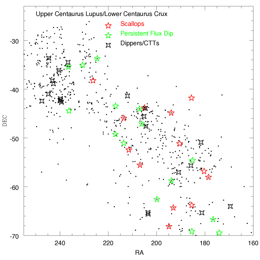
Figure 5: Spatial plot, showing the location on the sky of the candidate UCL/LCC members with TESS periods from our preliminary analysis of the ensemble. The stars in Tables 1 and 2 are plotted as five point star symbols. Additionally, stars identified as having CTT light curves (accretion bursts, AA Tau-like flux dips, or similar) are shown as four-point star symbols. The portion of UCL with RA $>235\arcdeg$ includes a significant population of CTTs but only two of our stars with highly structured light curves (the division between UCL and LCC is roughly at RA = 210$\arcdeg$, with UCL to the left in the plot and LCC to the right). This could indicate that the stars in that portion of UCL are, on average, younger than the stars in the other half of UCL or the stars in LCC.

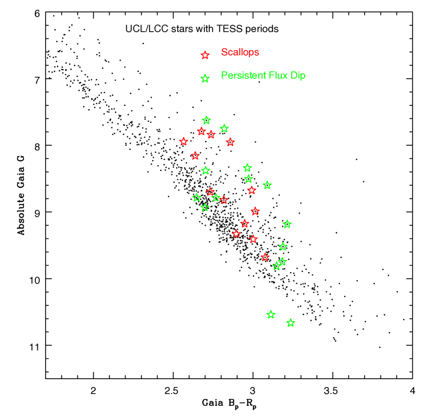
Figure 6: Absolute $G$ magnitude versus Gaia $B_{p}-R_{p}$ color for UCL/LCC candidate members from our preliminary analysis. The stars in Tables 1 and 2 are again plotted as star symbols. Many of the scallop-shell and persistent flux dip stars are well-displaced above the single-star locus in the diagram, either because they are younger or that they are members of binary systems.

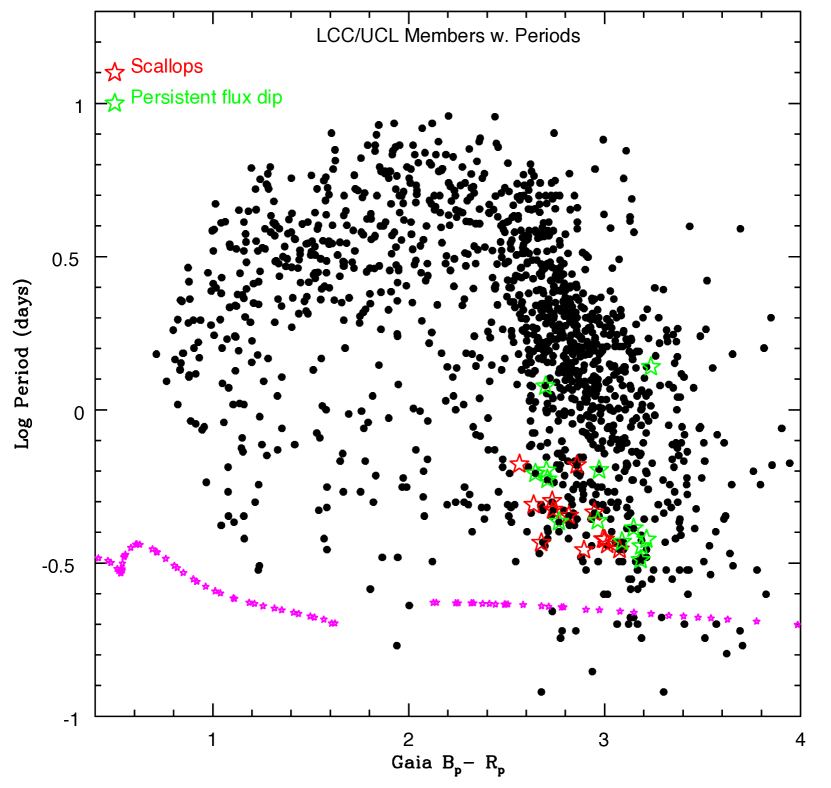
Figure 7: Log of the rotation period versus Gaia $B_{p}-R_{p}$ color for UCL/LCC candidate members from our preliminary analysis. The stars in Tables 1 and 2 are plotted as star symbols. The dashed magenta line shows an estimate of the rotational breakup rate, using the formula from Bouvier (2013) and the PARSEC 16 Myr isochrone. The scallop-shell and persistent flux dip stars are all rapid rotators, but their rotation periods are generally two or more times longer than the breakup rate.

If one places a tight box in Figure 8 around the stars of Table 1 and 2 (2.5 $<B_{p}-R_{p}<$ 3.2 and $-0.5<\log P<-0.1$), one can extract a set of rapidly rotating dM stars from our preliminary analysis possibly useful for comparison to the scallops and persistent flux dip stars. Doing so, and excluding our stars of interest, we find 110 such stars. The frequency for which a rapidly rotating dM stars shows the scallop/flux dip characteristics is then 28/138, or about 20%. We use this set of rapid rotators more in §8.

6 Comparison to the Scallop Shell Stars in Upper Sco

Despite being monitored by different satellites, the similarities between the scallop shell and persistent flux-dip stars in UCL/LCC, studied here with TESS, and those presented earlier in Upper Sco, based on K2 data, are substantial. For both datasets, the intrinsic faintness and distance of the stars of interest put those stars near the flux limit for TESS or K2 to provide useful light curves. Because UCL/LCC is older than Upper Sco, the stars of interest are intrinsically fainter; for LCC, that is compensated for by the closer mean distance to Earth, but UCL is about the same mean distance as Upper Sco and so our ability to identify scallop shell and flux-dip stars is most compromised there.

One possibly significant difference between UCL/LCC and Upper Sco is the ratio of scallop-shell to persistent flux-dip stars identified; in Upper Sco, that ratio is 15/8 or 1.8(${}^{+0.57}_{-0.34}$). In UCL/LCC, the ratio is 13/15 or 0.86(${}^{+0.05}_{-0.13}$). While small number statistics is a problem, this could suggest that the lifetime of scallop shells is significantly shorter than that for persistent flux-dip stars. The fact that a few persistent flux-dip stars are still present at Pleiades age (but no scallop shells with age $>$ 50 Myr are known) is consistent with this (Rebull et al. 2016b).

The period distributions in UCL/LCC for our stars with highly structured light curves are only slightly different from their cousins in Upper Sco. For Upper Sco, periods for scallops range from 0.26 day $<P<$ 0.78 day, with a median of 0.46 day; for the persistent flux dip stars, the period range is 0.48 day $<P<$ 1.54 day, with a median of 0.62 day. The same quantities for UCL/LCC (given in the previous section) are very similar. That may, in fact, be a little surprising given that low mass stars generally spin up on their path to the main sequence.

While we do not have spectral types in UCL/LCC, we do have accurate Gaia colors and we know there is little reddening (see, e.g., Pecaut & Mamajek 2016, where LCC and UCL have similar reddening based on 144 and 195 stars, respectively; dropping three anomalously high $A_{V}$ values from UCL, then the mean for both is $A_{V}\sim 0.15\pm$0.20). The Gaia $B_{p}-R_{p}$ colors for the scallops and persistent flux-dip stars imply spectral types ranging from M2.5 to M5. The measured spectral types in Upper Sco for scallops and persistent flux dip stars range from M3 to M6.3, with all but a couple being M5 or earlier. The red end of the spectral type range in both cases is almost certainly set by the photon count rates at K2 and TESS.

The amplitudes of variability in Upper Sco show the same wide range as in UCL/LCC, except that the maximum amplitude found in our sample was 21%, compared to the 15% in UCL/LCC. We find no significant difference in the flux dip depths or widths between the two groups.

7 Photometric Properties of the Stars in Tables 1 and 2

As described earlier, the lack of published data (e.g., spectra, high resolution imaging, etc) for our UCL/LCC stars limits our ability to attempt to use their properties to constrain possible theoretical models to explain their variability. However, UCL/LCC does have one very important positive attribute relative to Upper Sco. The low mass stars in Upper Sco have both relatively large reddening and large star-to-star reddening differences (see, e.g., discussion in Rebull et al. 2018 and references therein). The variable reddening adds considerable scatter to any diagram where color is used for one axis. UCL/LCC, on the other hand, has quite low reddening ($A_{V}\sim$ 0.15 mag). With the availability of the very accurate Gaia optical photometry and the good 2MASS and WISE near- and mid-IR photometry, it may be possible to identify color differences associated with our stars having highly structured light curves.

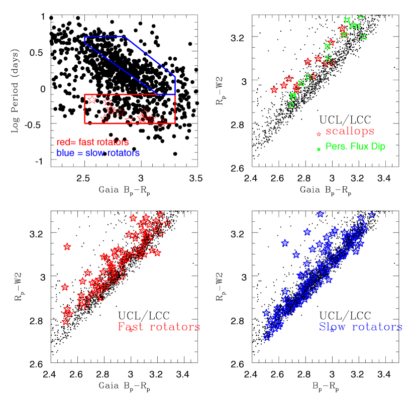
Figure 8: (a) log Period vs. color plot for dM members of UCL/LCC with periods; (b) $B_{p}-R_{p}$ vs. $R_{p}-[4.6]$ plot for the stars in panel (a), showing that the scallop shell light curves are systematically displaced from the bulk of the dMs; (c) similar plot for the rapid rotators; (d) similar plot for the slow rotators.

We have indeed found that there is a shared photometric anomaly among the rapidly rotating dM stars in UCL/LCC which may provide a clue to the photometric variability of the stars in Tables 1 and 2. Our evidence for this is provided in Figure 8. In order to investigate whether the rapid rotators in general (or the scallop shell stars in particular) have unusual photometric properties, we used a plot of period versus color to define several sets of stars, which we illustrate in the top-left panel of Figure 8. The stars with scallop-shell and persistent flux-dip morphology all have colors of 2.5 $<B_{p}-R_{p}<$ 3.3 and log $P$ between $-$0.1 and $-$0.5. All of the black dots in the plot represent the full sample of stars with periods from our preliminary analysis. The region outlined in blue defines the set of more slowly rotating stars; the region outlined in red defines the rapid rotators (from which we have removed all the stars in Tables 1 and 2). The top-right panel of Figure 8 compares the location in a plot of $B_{p}-R_{p}$ vs. $R_{p}-[4.6]$ (where [4.6] is the WISE-2 magnitude) for the scallops and persistent flux-dip stars versus the entire sample. Our stars of interest are clearly displaced either blueward in $B_{p}-R_{p}$ or redward in $R_{p}-[4.6]$ (or both) relative to the full sample. The bottom half of Figure 8 shows similar plots for the slowly rotating and fast rotating stars. The rapid rotators appear to be displaced from the main locus in a similar amount as for the scallops and persistent flux-dip stars; the slow rotators track the main locus of stars. The bottom line, therefore, is that all of the rapidly rotating, mid-to-late dM members have colors that are significantly different from slow rotators.

How can we interpret the color anomaly of the rapid rotators? If the displacement is primarily due to their having bluer $B_{p}-R_{p}$ colors, this could arise from their having a significant contribution to their light from hot spots (or plages). If the displacement is primarily due to their having redder $R_{p}-[4.6]$ colors, that could arise from their being a small amount of warm dust in the system. Unfortunately, without additional data, we cannot differentiate between those possibilities at this time.

8 TIC 242407571: There is Another Period

One of the most striking light curve morphologies shown in Figures 1-4 is the phased light curve for TIC 242407571. We reproduce that light curve here in Figure 9a. The most unusual and perplexing features of Fig. 9a are the icicle-like features “hanging” down from the scallop-shell waveform; the “icicles” appear to be both very narrow and reasonably equally spaced in phase. However, it is extremely unlikely that they are part of the scallop-shell waveform. None of the other stars in Tables 1 or 2 show features like this, nor, for that matter, for all of the Upper Sco (Rebull et al. 2018) stars we have discussed, nor in the rest of the stars in UCL and LCC (Rebull et al. in preparation), at least as part of our preliminary analysis. While we do not have a spectrum for TIC 242407571, its Gaia and 2MASS colors indicate that it should have a spectral type of about M4. Using the PARSEC 2.3 isochrone for a 16 Myr population, the Gaia color of $B_{p}-R_{p}$ = 2.737 converts to a mass of 0.40 M_☉, and an estimated radius of 0.80 M_☉. It is located well above the single star locus in the CMD shown in Figure 8, compatible with it being a nearly equal mass binary.

Figure 9: Various versions of the TIC 242407571 light curve, as described in the text.

In order to investigate the apparent icicles more closely, we have first made a fit to the scallop shell waveform, shown in Figure 9b. We then subtracted this fit from the original phased waveform, yielding the pure icicle light curve shown in Figure 9c. We retained the original MJD timestamps for each point during this process, and so we next ran a period search on this light curve using a box-least squares algorithm (also available at the NASA Exoplanet Archive Periodogram Service). A strong period of $P$ = 0.5681 day was found; Figure 9d shows the icicle light curve phased to this period. The phased light curve shows a relatively broad, apparently stable (in shape and depth) flux dip with a depth of about 2.5% and full-width zero intensity (FWZI) of about 0.22 in phase, plus two weaker outrigger flux dips separated by about 120 degrees in phase (on either side) from the primary dip.

How does the $P$=0.5681 day flux dip waveform result in the evenly spaced, nearly equal length icicle curtain shown in Figure 9a? There seems to be two primary drivers: a) the period of the flux dips and the period of the scallop-shell waveform have a ratio very close to 1.20 and b) the width of the main flux dip is wide enough that $\sim$4 TESS data samples are affected by the dip each period. For every five dip periods, there are six scallop-shell periods, and then the pattern repeats every $\sim$2.8 days. Because the ratio of the two periods (1.203) is very close to 6/5, the flux dips from the 0.568 day period align when phased to the 0.4721 day scallop-shell period, at least for the limited $\sim$20 day duration of each TESS campaign. If any one of the three parameters (TESS sampling frequency; ratio of the two periods; width of the flux dip) were significantly different, the evenly spaced, comb-tooth appearance of the icicles would not have happened.

We have created a simple model to illustrate this point, where we have replaced the scallop-shell waveform with a sine wave, and we have then added a flux dip at a different period from the light curve, retaining the exact observing cadence as for the real light curve. Figure 10 shows four instances of this model. In the top-left panel, a model with the same second period as the real star and a flux dip similar to the real flux dip was used; the resultant phased light curve shows icicles very similar to that observed. The top right panel shows the same model, except using a second period of 0.55 days, resulting in a random-appearing set of data points below the sine wave. The bottom left panel instead uses a period of 0.708 days, corresponding to 1.5 times the sine wave period of 0.4721d. We again see icicles, but of varying lengths and with a large gap between groups of them (the result of the dip width no longer being appropriate for the period ratio). Finally, the lower right panel shows what happens when the flux dip is made narrower; this results in icicles that are less well sampled.

Figure 10: Various versions of the model light curves, as described in the text.

Two questions immediately come to mind at this point. First, is the near alignment of the two periods by chance, or driven by some presumably gravitational process? Second, what is the nature of the material causing the flux dips which result in the 0.5681 day periodicity?

While having the two periods so well aligned (so that their ratio is near 1.20) would seem to suggest that a physical process was involved, there could be another interpretation. If the two periods were not so aligned, the 0.568 day flux dips would just result in a randomly positioned set of anomalously low points when phased to the 0.4721 day period (see Figure 10c). Our automated software did not pick up the 0.5681 day period because it provides too small a signal in the LS periodogram as compared to the signal from the scallop-shell waveform. Because we had to scan the plots for thousands of stars, it is possible our visual scanning of the phased light curves might have attributed the haze of low lying points as noise or data artifacts. Thus, the period alignment may have been an integral part of identifying this star as interesting – and other similar cases (but lacking an alignment to produce an ordered appearance of the low-lying points) may be present in other Sco-Cen light curves if analysed thoroughly.

The dip characteristics for TIC 242407571 are entirely compatible with what we have measured for the persistent flux dip stars in Table 2. Therefore, whatever physics is responsible for the persistent flux dip stars may well explain the $P$ = 0.5681 flux dips in TIC 242407571.

The model for TIC242407571 that has the fewest unusual assumptions is that it is in fact a binary system. One star exhibits the scallop shell light curve, and that star has a rotation period of 0.4721. The second star, which is probably a relatively wide binary companion, exhibits the $P$ = 0.5681 day persistent flux dip morphology. TIC242407571 is displaced well above the single star locus in Figure 8, in support of it being a binary. This model does not require any significant interaction between the two stars, and assumes that the fact that the ratio of their two periods of $\sim$1.20 is by chance. However, this star does not have exceptionally high astrometric excess noise nor exceptionally high re-normalised unit weight error.

9 Summary

By providing high quality, most-of-the-sky, deep, synoptic data for millions of stars, TESS is an ideal tool for discovering, or characterizing, new classes of photometric variability. We had previously used data from K2 to discover that some or perhaps all rapidly rotating mid-dM stars have highly structured light curves that could not be explained by any of the existing physical mechanisms inducing variability. In this paper, we have used TESS data to survey the light curves for thousands of low mass members of the UCL and LCC associations. We found nearly 30 of those stars are striking new examples of the light curve class we identified with K2. In Figures 1-4 we show phased-folded light curves for these stars, and in Figures 11-12 we provide plots of their SEDs.

The $B_{p}-R_{p}$ colors of the 28 UCL/LCC stars indicate that they have spectral types of M2.5 to M5. Their rotation rates range from 0.23 to 0.66 days; while quite rapid, except for two of the stars, those periods are more than a factor of two longer than the breakup period. Their amplitudes of variability range from a few percent to 15%; in particular, four of the scallop-shell stars have amplitudes of $\sim$15%. Such large amplitudes of variability will be a challenge for any of the physical mechanisms to explain.

The properties we have measured for this set of stars differ only slightly from those we had previously measured for the discovery set of objects in the Upper Sco association. The one most significant difference, perhaps, is the ratio of scallop shell to persistent flux dip stars – in Upper Sco, that ratio is 15/8, whereas in UCL/LCC the ratio is 13/15. One explanation would be that some stars have their light curve morphology evolve over time from more scallop-like to more flux-dip like. Another possibility is that the scallop-shell morphology has a shorter lifetime than the persistent flux dip morphology.

In §8, we have shown that the rapidly rotating low mass stars in UCL/LCC have colors that are either blue in $B_{p}-R_{p}$ or red in $R_{p}-[4.6]$ compared to the slowly rotating UCL/LCC members. The scallop-shell and persistent flux dip stars share those anomalous colors; their colors do not seem to stand out amongst the rapid rotators. Blue $B_{p}-R_{p}$ colors could arise if hot spots contribute significantly to the optical light from these stars. Red $R_{p}-[4.6]$ colors would most naturally arise if these stars had a small amount of warm dust.

What is most needed at this point is a viable physical mechanism that can recreate the variability properties we, and others, have measured. But observers can still help. Red-optical spectra to measure radial velocities and the H$\alpha$ emission profile at several phase points would be helpful. Multi-color, synoptic photometry of a few of the largest amplitude stars could help constrain dust grain properties. A survey for additional examples of this light curve class for a well-defined 30-40 Myr cluster or moving group would help determine the lifetimes of the scallops and persistent flux dip morphologies.

Appendix A Colors and Spectral Types

The correspondence between $B_{p}-R_{p}$ and spectral type that we are using is derived from the data in Table 3, where the spectral types come from the literature. All of the stars discussed here have $B_{p}-R_{p}$ 2.5 to 3.25, and are therefore taken to be M2.5 to M5.

Table 3: Correspondence between $B_{p}-R_{p}$ and spectral type

Object	Spectral Type	$B_{p}-R_{p}$
HII 2940	M0	1.75
HII 624	M2	2.23
HII 2601	M2	2.205
HII 2602	M2.5	2.435
HII 906	M3	2.387
MT 61	M3	2.889
HCG 456	M4	2.888
VA208	M4.6	3.299
VA203	M4.6	3.150
VA 362	M5	3.16
GJ905	M5	3.531
HHJ 6	$\sim$M6	3.512
VB8	M7	4.7542

Appendix B Spectral Energy Distributions

Spectral energy distributions for all the stars from Tables 1 and 2 are provided here as Figure 11 and Figure 12. Plots are log $\lambda F_{\lambda}$ in cgs units (ergs s^-1 cm^-2) against log $\lambda$ in microns. Symbols: black square at short bands: APASS; green square at short bands: Gaia DR2; black asterisk at short bands: Pan-STARRS1; $+$: optical other literature (NOMAD, SPM, etc. not already plotted); diamond: 2MASS $JHK_{s}$; circle: IRAC; black square at long bands: MIPS; stars: WISE from AllWISE; blue square in the mid-IR: CatWISE; green $+$ in the mid-IR: unWISE; arrows: limits; vertical bars (often smaller than the symbol) denote uncertainties. A line with a Rayleigh-Jeans slope is also shown as the dashed line, extended from the observations at $K_{s}$ when available, or WISE-1. Note that this is not a robust fit, but just to “guide the eye.” Almost all the stars have SEDs consistent with pure photospheres; none have large IR excesses.

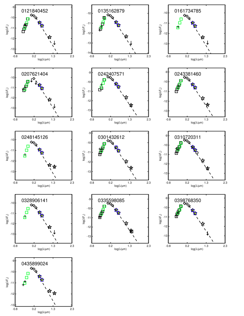
Figure 11: Spectral energy distributions for the stars in Table 1. See text for a description of the symbols.

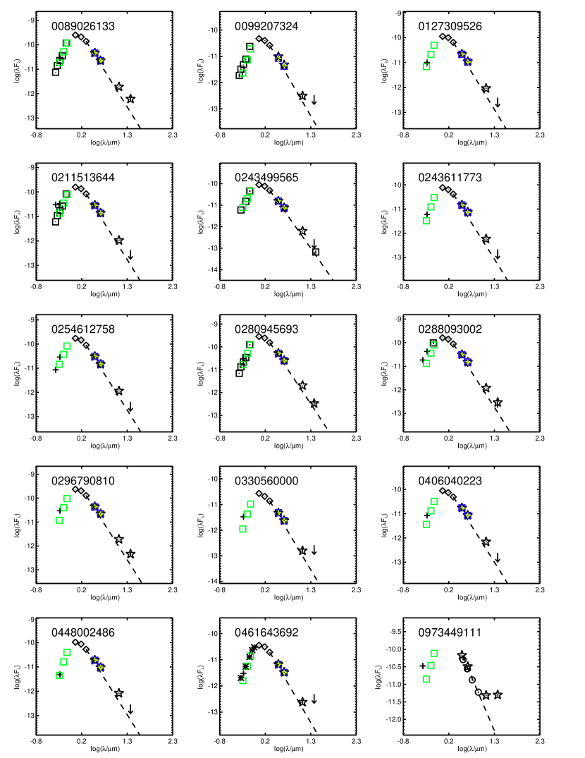
Figure 12: Spectral energy distributions for the stars in Table 2.

References

- Ahn et al. (2014) Ahn, C., Alexandroff, R., Allende Prieto, C., et al. 2014, ApJS, 211, 17
- Ansdell et al. (2020) Ansdell, M, Gaidos, E., Hedges, C., et al. 2020, MNRAS, 492, 572
- Bouma et al. (2019) Bouma, L., Hartman, J., Bhatt, W. et al. 2019, ApJS, 245, 13.
- Bouma et al. (2020) Bouma, L., Winn, J., Ricker, G. et al. 2020, AJ, 160, 86.
- Bouvier et al. (1999) Bouvier, J., Chelli, A., Carrasco, L., et al. 1999, A&A, 349, 619.
- Bouvier (2013) Bouvier, J. in “Angular momentum transport during the formation and early evolution of stars”, Hennebelle, P. & Charbonnel, C. (eds). 2011, ESA Pub. Series, 62, 143
- Chen et al. (2014) Chen, Y, Girardi, L., Bressan, A. et al. 2014, MNRAS, 444, 2525.
- Cody et al. (2014) Cody, A., Stauffer, J., Baglin, A., et al. 2014, AJ, 147, 82.
- Cutri et al. (2012) Cutri, R. M., Wright, E. L., Conrow, T., et al. 2012, http://wise2.ipac.caltech.edu/docs/release/allsky/expsup/
- Damiani et al. (2018) Damiani, F., Prisinzano, L., Pillitteri, I., et al. 2019, A&A, 623, 112.
- Eisenhardt et al. (2020) Eisenhardt, P., Marocco, F., Fowler, J., et al., 2020, ApJS, 247, 69
- Erickson et al. (2011) Erickson, K., Wilking, B., Meyer, M., et al. 2011, AJ, 142, 140.
- Feinstein et al. (2019) Feinstein, A., Montet, B., Foreman-Mackey, D. et al. 2019, PASP, 131, 4502.
- Gaia Collaboration et al. (2016) Gaia Collaboration, Brown, A., Vallenari, A., Prusti, T., de Bruijne, J.H.J., et al., 2016, A&A, 595, 2
- Gaia Collaboration et al. (2018) Gaia Collaboration, Brown, A., Vallenari, A., Prusti, T., de Bruijne, J.H.J., et al., 2018, A&A, 616, 1
- Girard et al. (2011) Girard, T., van Altena, W., Zacharias, N., Viera, K., et al., 2011, AJ, 142, 15
- Guenther etal. (2020) Güenther, M., Berardo, D., Ducrot, E., et al., 2020, AAS journals, submitted (arXiv:2008.11681)
- Henden & Munari (2014) Henden, A., & Munari, U., 2014, CoSka, 43, 518
- Howell et al. (2014) Howell, S., Sobeck, C., Haas, M., et al. 2014, PASP, 126, 398.
- Joy, A. (1945) Joy, A. 1945, ApJ, 102, 168.
- Kounkel, M. & Covey, K. (2019) Kounkel, M. & Covey, K. 2019, AJ, 158, 122.
- Lasker et al. (2008) Lasker, B., Lattanzi, M., McLean, B., et al., 2008, AJ, 136, 735
- Meisner et al. (2017) Meisner, A., Lang, D., Schlafly, E., & Schlegel, D., 2019, PASP, 131, 124504
- Morales-Calderon et al. (2011) Morales-Calderon,M., Stauffer, J., Hillenbrand, L. et al. 2011, ApJ, 733, 50.
- Murakami et al. (2007) Murakami, H., Baba,H., Barthel, P. et al. 2007, PASJ, 59, 369
- Pecaut & Mamajek (2016) Pecaut, M. & Mamajek, E. 2016, MNRAS, 461, 794.
- Ricker et al. (2015) Ricker, G. R., Winn, J. N., Vanderspek R., 2015, JATIS, 1, 014003
- Rebull et al. (2016a) Rebull, L., Stauffer, J., Bouvier, J., et al. 2016a, AJ, 152, 113.
- Rebull et al. (2016b) Rebull, L., Stauffer, J., Bouvier, J., et al. 2016b, AJ, 152, 114.
- Rebull et al. (2017) Rebull, L., Stauffer, J., Hillenbrand, L., et al. 2017, ApJ, 839,92.
- Rebull et al. (2018) Rebull, L., Stauffer, J., Cody, A., et al. 2018, AJ, 155, 196
- Rebull et al. (2020) Rebull, L., Stauffer, J., Cody, A., et al. 2020, AJ, 159, 273.
- Scargle (1982) Scargle, J. D. 1982, ApJ, 263, 835
- Skrutskie et al. (2006) Skrutskie, M., Cutri, R. M., Stiening, R., et al., 2006, AJ, 131, 1163
- Stauffer et al. (2018a) Stauffer, J., Rebull, L., Cody, A., et al. 2018a, AJ, 156, 275.
- Stauffer et al. (2018b) Stauffer, J., Rebull, L., David, T., et al. 2018b, AJ, 155, 63.
- Stauffer et al. (2017) Stauffer, J., Collier-Cameron, A., Jardine, M., et al. 2017, AJ, 153, 152.
- Stassun et al. (2018) Stassun, K., Oelkers, R., Pepper, J., et al. 2018, AJ, 156, 102
- Werner et al. (2004) Werner, M., Roellig, T., Low, F., et al., 2004, ApJS, 154, 1
- Wright et al. (2010) Wright, E., Eisenhardt, P. R. M., Mainzer, A. K., et al., 2010, AJ, 140, 1868
- Zacharias et al. (2004) Zacharias, N., Monet, D., Levine, S., et al., 2004, AAS, 205, 4815
- Zari et al. (2018) Zari, E., Hashemi, H., Brown, A.G.A. et al. 2018, A&A, 620, 172
- Zhan et al. (2019) Zhan, Z., Günther, M., Rappaportt, S., et al. 2019, ApJ, 876, 127