Paradoxical predictions
of liquid curtains with surface tension

Abstract

This paper examines two-dimensional liquid curtains ejected at an angle to the horizontal and affected by gravity and surface tension. The flow is, to leading order, shearless and viscosity, negligible. The Froude number is large, so that the radius of the curtain’s curvature exceeds its thickness. The Weber number is close to unity, so that the forces of inertia and surface tension are almost perfectly balanced. An asymptotic equation is derived under these assumptions, and its steady solutions are explored. It is shown that, for a given pair of ejection velocity/angle, infinitely many solutions exist, each representing a steady curtain with a stationary capillary wave superposed on it. These solutions describe a rich variety of behaviours: in addition to arching downwards, curtains can zigzag downwards, self-intersect, and even rise until the initial supply of the liquid’s kinetic energy is used up. The last type of solutions corresponds to a separatrix between upward- and downward-bending curtains – in both cases, self-intersecting (such solutions are meaningful only until the first intersection, after which the liquid just splashes down). Finally, suggestions are made as to how the existence of upward-bending curtains can be tested experimentally.

1 Introduction

A vertical liquid curtain can be created by cutting a long slot of constant width in the bottom of a tank; once the tank is filled, a flat liquid sheet will be squeezed through the slot. If the tank is tipped, the liquid will be squeezed obliquely, and the curtain’s trajectory will be curved due to gravity. Liquid curtains have important industrial applications (e.g., manufacturing of paper), but they are also part of classical fluid mechanics and, as such, have been studied for more than sixty years.

The present paper looks into a highly counter-intuitive phenomenon, so far examined only theoretically: that of oblique curtains bending upwards, i.e., against gravity.

The first such example was produced by KellerWeitz57 using a set of equations for a slender oblique curtain without shear and viscosity, but affected by gravity and surface tension. It was shown that all curtains with the ejection velocity below a certain threshold would bend upwards regardless of the ejection angle. The threshold corresponds to the Weber number $We$ being equal to unity ($We$ is the ratio of forces of inertia and surface tension). Keller & Weitz interpreted their paradoxical result using an analogy with a body affected by gravity and an extra force proportional to the acceleration.

Unfortunately, this thought-provoking work has been virtually forgotten: since 1957, it has been cited only 8 times. As a result, upward-bending curtains have been rediscovered – albeit in a more general formulation including shear and viscosity by Benilov19 (hereinafter, B19). This paper confirmed the criterion $We<1$ subject to a suitably modified definition of $We$ for sheared flows. Solutions describing upward-bending jets have been found by Wallwork01, but these are strongly unstable due to the Plateau–Rayleigh instability and, thus, cannot be observed experimentally.

The results obtained in B19 (and, by association, those of Keller & Weitz) have been criticised by WeinsteinRossRuschakBarlow19, who put forward the following claims:

1. For upward-bending curtains, the hyperbolic second-order set derived in B19 is such that one of the two characteristics corresponds to waves propagating upstream – i.e., towards the outlet, were the boundary conditions are set. Thus, “in accordance with hyperbolic theory” one of the two boundary conditions at the outlet must be omitted – namely, the one prescribing the ejection angle $\alpha_{0}$.

2. The omitted boundary condition should be replaced with $\alpha_{0}=-90^{\circ}$ corresponding to a vertical curtain.

It turns out that (1) is a valid point, whereas (2) is not.

That is, mathematically, there is no reason why a boundary condition cannot be formulated at a point other than the beginning of a characteristic (as long as there is only one such point per characteristic). Physically, however, such a condition would be in conflict with the causality principle, as it would effectively constrain events occurring in the past.

As for point (2), Weinstein et al. justified it by claiming that the condition $\alpha_{0}=-90^{\circ}$ “is precisely that necessary to eliminate the singularity in the curtain”. However, B19 found regular solutions for all values of $\alpha_{0}$, and earlier in their paper Weinstein et al. did not dispute their existence. One might add that it is inconsistent to use point (1) to discard one of the boundary conditions and then replace it with a similar one, leaving their total number exactly the same.

Even more importantly, the replacement of the actual ejection angle with $-90^{\circ}$ implies a sharp bend in the curtain near the outlet, and it cannot be caused by the force of gravity. If it were, the asymptotic models of both Weinstein et al. and B19 would have detected it (as they both include gravity) – hence, there would be no need to introduce the turn through the boundary condition. Nor can it be caused by other hydrodynamic effects, as they are all isotropic and, thus, cannot make the curtain ‘choose’ the vertical trajectory regardless of the ejection angle (not to mention that the only significant ones of these effects – viscosity and surface tension – are also included in the B19 model).

Still, one question remains: if the solutions found in B19 for upward-bending curtains are indeed physically meaningless, what really happens if liquid is ejected obliquely with $We<1$?

The present paper offers a possible answer to this question through an analysis of the simplest setting: that of ideal fluid and almost shearless curtains. The Weber number is assumed to be close to unity, in which case the phase velocity of the upstream capillary waves is small, so that their dispersion comes into play. Since the velocity of dispersive waves is not bounded above, events occurring anywhere in the curtain are immediately sensed near the outlet, thus resolving the conflict with the causality principle.

Mathematically, the asymptotic limit $We\approx 1$ invalidates all of the existing models of oblique liquid curtains (including KellerWeitz57; FinnicumWeinsteinRuschak93; Benilov19): the leading-order terms almost cancel each other, so the previously-discarded next-order terms have to be taken into account (as was done by Ramos03 for vertical curtains). Once the correct equation for this limit is derived, one can see that it is not hyperbolic: it involves a first-order time derivative and a third-order spatial derivative (similarly to the Korteweg–de Vries equation for gravity-capillary waves in shallow water). As a result, the whole notion of characteristics becomes irrelevant.

The equation derived will be used to examine steady curtains, and it will be shown that some of them do bend upwards and rise until all of the liquid’s kinetic energy is used up (and the asymptotic governing equation becomes inapplicable); other curtains rise until they are truncated by a self-intersection. There are also solutions describing downward-bending curtains, both infinite and self-intersecting.

Interestingly, the model seems to ‘know’ that it becomes almost hyperbolic when the deviation of $We$ from unity is order-one: subcritical ($We<1$) solutions in this case are highly sensitive to small variations of the parameters involved, with both upward- and downward-bending curtains often self-intersecting very near the outlet. One can assume that they are structurally unstable – hence, physically meaningless – and the flow in this case is unlikely to settle down into a steady curtain. But near-critical curtains, including subcritical ones, could be observable. Admittedly, this does not conclusively follow from their existence as steady solutions of the governing equations (which is shown in this paper), as one should also prove their stability (which has yet to be done).

The present paper has the following structure: in §2, we formulate the problem and, in §3, derive an asymptotic equation for curtains with a large Froude number and near-unity Weber number. Steady solutions of this equation are examined in §4 and their physical aspects (e.g., how to create an upward-bending curtain in an experiment), in §5.

2 Formulation of the problem

2.1 Governing equations

Consider an incompressible ideal fluid of density $\rho$ ejected from an infinitely long horizontal slot (outlet) of fixed width. Let the flow be homogeneous in the along-the-outlet direction – i.e., depend on a single horizontal coordinate $x$ and the vertical coordinate $z$ (see figure 1).

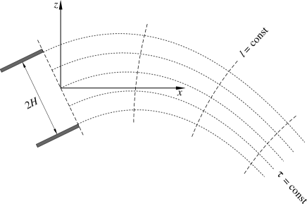
Figure 1: The setting: a two-dimensional liquid curtain ejected from an outlet of width $2H$. $\left(x,z\right)$ are the Cartesian coordinates and $\left(l,\tau\right)$ are the curvilinear coordinates associated with the curtain’s centreline (corresponding to $\tau=0$).
       The important quantities not shown in the figure: the local angle $\alpha(l,t)$ between the centreline and the horizontal, its near-outlet value $\alpha_{0}$ (determined by the outlet’s orientation – hence, time-independent), and the near-outlet curvature $\alpha_{0}^{\prime}(t)=\left(\partial\alpha/\partial l\right)_{l=0}$.

Unless the liquid is ejected vertically, the curtain’s trajectory is curved due to gravity, making the Cartesian coordinates awkward to use. It is more convenient to employ curvilinear coordinates associated with the curtain’s centreline (EntovYarin84; Wallwork01; WallworkDecentKingSchulkes02; ShikhmurzaevSisoev17; DecentParauSimmonsUddin18; Benilov19).

Consider curvilinear coordinates $\left(l,\tau\right)$ related to their Cartesian counterparts by

$$x=x(l,\tau,t),\qquad z=z(l,\tau,t),$$

where $t$ is the time. Let the set $\left(l,\tau\right)$ be orthogonal with a unit Jacobian,

$$\frac{\partial x}{\partial l}\frac{\partial x}{\partial\tau}+\frac{\partial z}{\partial l}\frac{\partial z}{\partial\tau}=0,\qquad\frac{\partial x}{\partial l}\frac{\partial z}{\partial\tau}-\frac{\partial x}{\partial\tau}\frac{\partial z}{\partial l}=1.$$ (1)

Since the solution of equations (1) is not constrained by boundary conditions, the relationship between $\left(x,z\right)$ and $\left(l,\tau\right)$ is not unique, leaving one an opportunity to choose the set $\left(l,\tau\right)$ that makes the forthcoming calculations simpler.

In what follows, the so-called Lamé coefficients

$$h_{l}=\sqrt{\left(\frac{\partial x}{\partial l}\right)^{2}+\left(\frac{\partial z}{\partial l}\right)^{2}},\qquad h_{\tau}=\sqrt{\left(\frac{\partial x}{\partial\tau}\right)^{2}+\left(\frac{\partial z}{\partial\tau}\right)^{2}}$$ (2)

will be needed. It follows from (1) that $h_{l}h_{\tau}=1$, i.e., the transformation $\left(x,z\right)\rightarrow\left(l,\tau\right)$ preserves the elemental area.

Let the flow be characterised by the velocity components $\left(u_{l},u_{\tau}\right)$ and the pressure $p$. Representing the gravitational force by $-\rho g\mathbf{\nabla}z$ ($g$ is the acceleration due to gravity), one can write the Euler equations in the form

$$h_{l}\frac{\partial u_{l}}{\partial t}+\left[u_{l}-\frac{1}{h_{l}}\left(\frac{\partial x}{\partial l}\frac{\partial x}{\partial t}+\frac{\partial z}{\partial l}\frac{\partial z}{\partial t}\right)\right]\left(\frac{\partial u_{l}}{\partial l}+\frac{u_{\tau}}{h_{\tau}}\dfrac{\partial h_{l}}{\partial\tau}\right)\\ +\frac{h_{l}}{h_{\tau}}\left[u_{\tau}-\frac{1}{h_{\tau}}\left(\frac{\partial x}{\partial\tau}\frac{\partial x}{\partial t}+\frac{\partial z}{\partial\tau}\frac{\partial z}{\partial t}\right)\right]\frac{\partial u_{l}}{\partial\tau}\\ +\frac{u_{\tau}}{h_{\tau}}\left[\dfrac{\partial x}{\partial l}\frac{\partial^{2}x}{\partial t\,\partial\tau}+\dfrac{\partial z}{\partial l}\frac{\partial^{2}z}{\partial t\,\partial\tau}-\frac{1}{h_{\tau}^{2}}\left(\frac{\partial x}{\partial\tau}\frac{\partial x}{\partial t}+\frac{\partial z}{\partial\tau}\frac{\partial z}{\partial t}\right)\left(\dfrac{\partial x}{\partial l}\frac{\partial^{2}x}{\partial\tau^{2}}+\dfrac{\partial z}{\partial l}\frac{\partial^{2}z}{\partial\tau^{2}}\right)-u_{\tau}\frac{\partial h_{\tau}}{\partial l}\right]\\ +\dfrac{1}{\rho}\dfrac{\partial p}{\partial l}=-g\dfrac{\partial z}{\partial l},$$ (3)

$$h_{\tau}\frac{\partial u_{\tau}}{\partial t}+\frac{h_{\tau}}{h_{l}}\left[u_{l}-\frac{1}{h_{l}}\left(\frac{\partial x}{\partial l}\frac{\partial x}{\partial t}+\frac{\partial z}{\partial l}\frac{\partial z}{\partial t}\right)\right]\frac{\partial u_{\tau}}{\partial l}\\ +\left[u_{\tau}-\frac{1}{h_{\tau}}\left(\frac{\partial x}{\partial\tau}\frac{\partial x}{\partial t}+\frac{\partial z}{\partial\tau}\frac{\partial z}{\partial t}\right)\right]\left(\frac{\partial u_{\tau}}{\partial\tau}+\frac{u_{l}}{h_{l}}\frac{\partial h_{\tau}}{\partial l}\right)\\ +\frac{u_{l}}{h_{l}}\left[\dfrac{\partial x}{\partial\tau}\frac{\partial^{2}x}{\partial t\,\partial l}+\dfrac{\partial z}{\partial\tau}\frac{\partial^{2}z}{\partial t\,\partial l}-\frac{1}{h_{l}^{2}}\left(\frac{\partial x}{\partial l}\frac{\partial x}{\partial t}+\frac{\partial z}{\partial l}\frac{\partial z}{\partial t}\right)\left(\dfrac{\partial x}{\partial\tau}\frac{\partial^{2}x}{\partial l^{2}}+\dfrac{\partial z}{\partial\tau}\frac{\partial^{2}z}{\partial l^{2}}\right)-u_{l}\frac{\partial h_{l}}{\partial\tau}\right]\\ +\dfrac{1}{\rho}\dfrac{\partial p}{\partial\tau}=-g\dfrac{\partial z}{\partial\tau},$$ (4)

$$\frac{\partial\left(u_{l}h_{\tau}\right)}{\partial l}+\frac{\partial\left(u_{\tau}h_{l}\right)}{\partial\tau}=0.$$ (5)

For a stationary coordinate system (such that $\partial x/\partial l=\partial x/\partial t=0$), equations (3)–(5) can be found in most textbooks (e.g. KochinKibelRoze64), with the general case considered in B19.

Let the liquid be bounded by two free surfaces described by equations $\tau=\tau_{-}(l,t)$ and $\tau=\tau_{+}(l,t)$, where the functions $\tau_{\pm}(l,\tau)$ satisfy the free-boundary kinematic condition. If written in terms of time-dependent curvilinear coordinates, it takes the form

$$\frac{\partial\tau_{\pm}}{\partial t}+\frac{1}{h_{l}}\left[u_{l}-\dfrac{1}{h_{l}}\left(\frac{\partial x}{\partial l}\frac{\partial x}{\partial t}+\frac{\partial z}{\partial l}\frac{\partial z}{\partial t}\right)\right]\dfrac{\partial\tau_{\pm}}{\partial l}\\ -\frac{1}{h_{\tau}}\left[u_{\tau}-\dfrac{1}{h_{\tau}}\left(\frac{\partial x}{\partial\tau}\frac{\partial x}{\partial t}+\frac{\partial z}{\partial\tau}\frac{\partial z}{\partial t}\right)\right]=0\qquad\text{if}\qquad\tau=\tau_{\pm}.$$ (6)

The dynamic boundary condition, in turn, assumes that the pressure at a free boundary is determined by its curvature and surface tension $\sigma$,

$$p=\mp\sigma\left\{\frac{\partial}{\partial l}\left[\frac{\dfrac{h_{\tau}^{2}}{h_{l}}\dfrac{\partial\tau_{\pm}}{\partial l}}{\sqrt{1+\left(\dfrac{h_{\tau}}{h_{l}}\dfrac{\partial\tau_{\pm}}{\partial l}\right)^{2}}}\right]-\frac{\partial}{\partial\tau}\left[\frac{h_{l}}{\sqrt{1+\left(\dfrac{h_{\tau}}{h_{l}}\dfrac{\partial\tau_{\pm}}{\partial l}\right)^{2}}}\right]\right\}\qquad\text{if}\qquad\tau=\tau_{\pm}$$ (7)

(for more details on conditions (6)–(7), see B19).

Let the outlet’s width be $2H$. In this paper, the simplest particular case is examined, where the streamwise component of the velocity at the outlet is not sheared (i.e., is independent of $\tau$), while the cross-stream component is identically zero,

$$u_{l}=u_{0},\qquad u_{\tau}=0\qquad\text{if}\qquad l=0,\qquad\tau\in\left(-H,H\right),$$ (8)

where $u_{0}$ may depend on $t$. The outlet conditions for the curtain’s boundaries are, obviously,

$$\tau_{\pm}=\pm H\qquad\text{if}\qquad l=0.$$ (9)

Given an initial condition and a specific solution of the coordinate equations (1), the boundary-value problem (2)–(9) (presumably uniquely) determines $p$, $u_{l}$, $u_{\tau}$, and $\tau_{\pm}$.

It is convenient to identify the curtain’s centreline with the curve $\tau=0$. To do so, require that

$$\tau_{\pm}=\pm W,$$ (10)

where $W(l,t)$ is the curtain’s half-width.

2.2 The scaling

There are two nondimensional parameters in the problem at hand. The Froude number

$$Fr=\frac{u_{0}^{2}}{gH},$$

reflects the balance of inertia and gravity, and the Weber number

$$We=\frac{\rho Hu_{0}^{2}}{\sigma}$$

that of inertia and surface tension. This paper is concerned the limit $We\approx 1$, which implies that the velocity should be scaled by

$$U=\left(\frac{\sigma}{\rho H}\right)^{1/2}.$$ (11)

In B19, the curtain’s spatial scale $L$ was derived from the assumption that the centrifugal force (due to the curtain’s curvature), surface tension, and gravity are in balance – which implies that $L=H\,Fr$, so that the slender-curtain approximation is valid if $Fr\gg 1$.

If, however, $We\rightarrow 1$, the leading-order surface tension and centrifugal force tend to cancel each other. As a result, gravity remains unopposed and makes the curtain bend much more steeply (see figure 2 in B19).

To determine $L$ for the case $We\approx 1$, one should balance gravity with higher-order corrections to centrifugal force and surface tension – which have to be calculated first, of course – which is, however, impossible without a conjecture as to what $L$ actually is. This task is exacerbated even more by the fact that the next-to-leading-order corrections do contribute to the eventual asymptotic equation, forcing one to delve into yet another order.

Thus, $L$ was effectively determined through a trial-and-error approach, and it has turned out that a consistent asymptotic theory can be derived if

$$L=\frac{H}{\epsilon},$$ (12)

where $\epsilon$ is the cube root of the Bond number,

$$\epsilon=\left(\frac{\rho gH^{2}}{\sigma}\right)^{1/3},$$ (13)

or, equivalently, $\epsilon=\left(We/Fr\right)^{1/3}\approx Fr^{-1/3}$.

In the present paper, $\epsilon$ is assumed small – hence, $L\gg H$. The larger scale, $L$, will be used to nondimensionalise the Cartesian coordinates $\left(x,z\right)$ and the streamwise variable $l$, whereas the cross-stream variable $\tau$ and the curtain’s half-width $W$ will be nondimensionalised by $H$.

The following nondimensional variables will be used:

$$\left.\begin{array}[]{c}l_{nd}=\dfrac{l}{L},\qquad\tau_{nd}=\dfrac{\tau}{H},\qquad t_{nd}=\dfrac{t}{T},\qquad x_{nd}=\dfrac{x}{L},\qquad z_{nd}=\dfrac{z}{L},\vskip 6.0pt plus 2.0pt minus 2.0pt\\ \left(u_{l}\right)_{nd}=\dfrac{u_{l}}{U},\qquad\left(u_{\tau}\right)_{nd}=\dfrac{u_{\tau}}{\epsilon^{2}U},\qquad p_{nd}=\dfrac{p}{P},\qquad W_{nd}=\dfrac{W}{H}.\end{array}\right\}$$ (14)

The pressure scale $P$ is such that the centrifugal force is, to leading order, balanced by the capillary-pressure gradient, which implies

$$P=\frac{\rho gH}{\epsilon^{2}}.$$ (15)

The time scale $T$ is determined by the balance of the Coriolis force and gravity – i.e., the time derivatives of $x$ and $z$ in equation (4) and its right-hand side, respectively – which amounts to

$$T=\frac{H}{\epsilon^{3}U}.$$ (16)

Rewriting (1)–(7) in terms of variables (14)–(16), taking into account (11)–(13), and omitting the subscript _nd, one obtains

$$\frac{\partial x}{\partial l}\frac{\partial x}{\partial\tau}+\frac{\partial z}{\partial l}\frac{\partial z}{\partial\tau}=0,\qquad\frac{1}{\epsilon}\left(\frac{\partial x}{\partial l}\frac{\partial z}{\partial\tau}-\frac{\partial x}{\partial\tau}\frac{\partial z}{\partial l}\right)=1,$$ (17)

$$h_{l}=\sqrt{\left(\frac{\partial x}{\partial l}\right)^{2}+\left(\frac{\partial z}{\partial l}\right)^{2}},\qquad h_{\tau}=\frac{1}{\epsilon}\sqrt{\left(\frac{\partial x}{\partial\tau}\right)^{2}+\left(\frac{\partial z}{\partial\tau}\right)^{2}},$$ (18)

$$\epsilon h_{l}\frac{\partial u_{l}}{\partial t}+\left[u_{l}-\frac{\epsilon^{2}}{h_{l}}\left(\frac{\partial x}{\partial l}\frac{\partial x}{\partial t}+\frac{\partial z}{\partial l}\frac{\partial z}{\partial t}\right)\right]\left(\frac{1}{\epsilon}\frac{\partial u_{l}}{\partial l}+\frac{u_{\tau}}{h_{\tau}}\dfrac{\partial h_{l}}{\partial\tau}\right)\\ +\frac{h_{l}}{h_{\tau}}\left[u_{\tau}-\frac{1}{\epsilon h_{\tau}}\left(\frac{\partial x}{\partial\tau}\frac{\partial x}{\partial t}+\frac{\partial z}{\partial\tau}\frac{\partial z}{\partial t}\right)\right]\frac{\partial u_{l}}{\partial\tau}\\ +\frac{\epsilon^{2}u_{\tau}}{h_{\tau}}\left[\dfrac{\partial x}{\partial l}\frac{\partial^{2}x}{\partial t\,\partial\tau}+\dfrac{\partial z}{\partial l}\frac{\partial^{2}z}{\partial t\,\partial\tau}-\frac{1}{\epsilon^{2}h_{\tau}^{2}}\left(\frac{\partial x}{\partial\tau}\frac{\partial x}{\partial t}+\frac{\partial z}{\partial\tau}\frac{\partial z}{\partial t}\right)\left(\dfrac{\partial x}{\partial l}\frac{\partial^{2}x}{\partial\tau^{2}}+\dfrac{\partial z}{\partial l}\frac{\partial^{2}z}{\partial\tau^{2}}\right)-\epsilon u_{\tau}\frac{\partial h_{\tau}}{\partial l}\right]\\ +\frac{\partial p}{\partial l}=-\epsilon\dfrac{\partial z}{\partial l},$$ (19)

$$\epsilon^{4}h_{\tau}\frac{\partial u_{\tau}}{\partial t}+\frac{\epsilon^{2}h_{\tau}}{h_{l}}\left[u_{l}-\frac{\epsilon^{2}}{h_{l}}\left(\frac{\partial x}{\partial l}\frac{\partial x}{\partial t}+\frac{\partial z}{\partial l}\frac{\partial z}{\partial t}\right)\right]\frac{\partial u_{\tau}}{\partial l}\\ +\epsilon^{3}\left[u_{\tau}-\frac{1}{\epsilon h_{\tau}}\left(\frac{\partial x}{\partial\tau}\frac{\partial x}{\partial t}+\frac{\partial z}{\partial\tau}\frac{\partial z}{\partial t}\right)\right]\left(\frac{\partial u_{\tau}}{\partial\tau}+\frac{u_{l}}{\epsilon h_{l}}\frac{\partial h_{\tau}}{\partial l}\right)\\ +\frac{u_{l}}{h_{l}}\left[\epsilon\left(\dfrac{\partial x}{\partial\tau}\frac{\partial^{2}x}{\partial t\,\partial l}+\dfrac{\partial z}{\partial\tau}\frac{\partial^{2}z}{\partial t\,\partial l}\right)-\frac{\epsilon}{h_{l}^{2}}\left(\frac{\partial x}{\partial l}\frac{\partial x}{\partial t}+\frac{\partial z}{\partial l}\frac{\partial z}{\partial t}\right)\left(\dfrac{\partial x}{\partial\tau}\frac{\partial^{2}x}{\partial l^{2}}+\dfrac{\partial z}{\partial\tau}\frac{\partial^{2}z}{\partial l^{2}}\right)-\frac{u_{l}}{\epsilon}\frac{\partial h_{l}}{\partial\tau}\right]\\ +\frac{\partial p}{\partial\tau}=-\epsilon\dfrac{\partial z}{\partial\tau},$$ (20)

$$\frac{1}{\epsilon}\frac{\partial\left(u_{l}h_{\tau}\right)}{\partial l}+\frac{\partial\left(u_{\tau}h_{l}\right)}{\partial\tau}=0,$$ (21)

$$\epsilon\frac{\partial W}{\partial t}+\dfrac{1}{\epsilon h_{l}}\left[u_{l}-\dfrac{\epsilon^{2}}{h_{l}}\left(\frac{\partial x}{\partial l}\frac{\partial x}{\partial t}+\frac{\partial z}{\partial l}\frac{\partial z}{\partial t}\right)\right]\dfrac{\partial W}{\partial l}\\ \mp\frac{1}{h_{\tau}}\left[u_{\tau}-\dfrac{1}{\epsilon h_{\tau}}\left(\frac{\partial x}{\partial\tau}\frac{\partial x}{\partial t}+\frac{\partial z}{\partial\tau}\frac{\partial z}{\partial t}\right)\right]=0\qquad\text{if}\qquad\tau=\pm W,$$ (22)

$$p=-\epsilon\frac{\partial}{\partial l}\left[\frac{\dfrac{h_{\tau}^{2}}{h_{l}}\dfrac{\partial W}{\partial l}}{\sqrt{1+\left(\dfrac{\epsilon h_{\tau}}{h_{l}}\dfrac{\partial W}{\partial l}\right)^{2}}}\right]\pm\frac{1}{\epsilon}\frac{\partial}{\partial\tau}\left[\frac{h_{l}}{\sqrt{1+\left(\dfrac{\epsilon h_{\tau}}{h_{l}}\dfrac{\partial W}{\partial l}\right)^{2}}}\right]\qquad\text{if}\qquad\tau=\pm W,$$ (23)

When nondimensionalising the boundary conditions (8)–(9), it is convenient to introduce the nondimensional ‘excess injection velocity’ $v_{0}$ such that

$$u_{0}=U\left(1+\epsilon^{2}v_{0}\right).$$ (24)

Then, (8) becomes

$$u_{l}=1+\epsilon^{2}v_{0},\qquad u_{\tau}=0\qquad\text{if}\qquad l=0,\qquad\tau\in\left(-1,1\right).$$ (25)

Finally, the nondimensional version of the boundary condition (9)–(10), is

$$W=1\qquad\text{if}\qquad l=0.$$ (26)

2.3 How should the curvilinear coordinates be chosen?

As stated before, the curvilinear coordinates $\left(l,\tau\right)$ are associated with the curtain’s centreline – but this association has not been reflected in the general equations (17) relating $\left(l,\tau\right)$ to the Cartesian coordinates.

To single out the desired solution of (17), introduce the centreline’s Cartesian coordinates $x=\bar{x}(l,t)$ and $z=\bar{z}(l,t)$, and the local angle $\alpha(l,t)$ between the centreline and the horizontal. Let $l$ be the centreline’s arclength, which implies

$$\frac{\partial\bar{x}}{\partial l}=\cos\alpha,\qquad\frac{\partial\bar{z}}{\partial l}=\sin\alpha,$$ (27)

$$\bar{x}=0,\qquad\bar{z}=0\qquad\text{if}\qquad l=0.$$ (28)

For a given $\alpha(l,t)$, (27)–(28) uniquely determine $\bar{x}(l,t)$ and $\bar{z}(l,t)$.

Now, seek a solution (17) in the form of a series in powers of $\left(\epsilon\tau\right)$, with the zero-order terms in the expansions of $x$ and $z$ being $\bar{x}(l)$ and $\bar{z}(l)$, respectively. After straightforward algebra (for more detail, see B19), one obtains

$$x=\bar{x}-\epsilon\tau\sin\alpha-\frac{(\epsilon\tau)^{2}}{2}\frac{\partial\alpha}{\partial l}\sin\alpha-(\epsilon\tau)^{3}\left[\frac{1}{6}\frac{\partial^{2}\alpha}{\partial l^{2}}\cos\alpha+\frac{1}{2}\left(\frac{\partial\alpha}{\partial l}\right)^{2}\sin\alpha\right]+\mathcal{O}(\epsilon^{4}),$$ (29)

$$z=\bar{z}+\epsilon\tau\cos\alpha+\frac{(\epsilon\tau)^{2}}{2}\frac{\partial\alpha}{\partial l}\cos\alpha-(\epsilon\tau)^{3}\left[\frac{1}{6}\frac{\partial^{2}\alpha}{\partial l^{2}}\sin\alpha-\frac{1}{2}\left(\frac{\partial\alpha}{\partial l}\right)^{2}\cos\alpha\right]+\mathcal{O}(\epsilon^{4}).$$ (30)

Substitution of these expressions into (18) yields the following expressions for the Lamé coefficients:

$$h_{l}=1-\epsilon\tau\frac{\partial\alpha}{\partial l}-\frac{(\epsilon\tau)^{2}}{2}\left(\frac{\partial\alpha}{\partial l}\right)^{2}-(\epsilon\tau)^{3}\left[\frac{1}{6}\frac{\partial^{3}\alpha}{\partial l^{3}}+\frac{1}{2}\left(\frac{\partial\alpha}{\partial l}\right)^{3}\right]+\mathcal{O}(\epsilon^{4}),$$ (31)

$$h_{\tau}=1+\epsilon\tau\frac{\partial\alpha}{\partial l}+\frac{3(\epsilon\tau)^{2}}{2}\left(\frac{\partial\alpha}{\partial l}\right)^{2}+(\epsilon\tau)^{3}\left[\frac{1}{6}\frac{\partial^{3}\alpha}{\partial l^{3}}+\frac{5}{2}\left(\frac{\partial\alpha}{\partial l}\right)^{3}\right]+\mathcal{O}(\epsilon^{4}).$$ (32)

3 Asymptotic analysis

The sheer size of the governing equations makes their analysis cumbersome. To mitigate this problem, the asymptotic results and their physical meaning will be summarised first, in §3.1, with the technicalities described in §§3.2–3.4.

3.1 Summary

All characteristics of the flow can be related to the curtain’s coordinates $\bar{x}(l,t)$ and $\bar{z}(l,t)$, and the local angle $\alpha(l,t)$ between its centreline and the horizontal. The former satisfy (27)–(28), and the latter is governed by the following asymptotic equation:

$$\frac{\partial\alpha}{\partial t}+\frac{\partial\alpha}{\partial l}\left[v_{0}-\frac{1}{2}\bar{z}+\frac{1}{12}\left(\frac{\partial\alpha}{\partial l}\right)^{2}-\frac{1}{6}\alpha_{0}^{\prime 2}\right]+\frac{1}{6}\frac{\partial^{3}\alpha}{\partial l^{3}}=-\frac{1}{2}\cos\alpha,$$ (33)

where $v_{0}$ is the excess injection velocity [see (25)] and

$$\alpha_{0}^{\prime}=\left(\frac{\partial\alpha}{\partial l}\right)_{l=0}$$ (34)

is the curtain’s curvature near the outlet. This characteristic plays an important role in the curtain’s global dynamics.

Equation (33) requires two boundary conditions at the outlet, with one of these prescribing the ejection angle,

$$\alpha=\alpha_{0}\qquad\text{if}\qquad l=0,$$ (35)

where $\alpha_{0}$ may vary with $t$. An additional boundary condition follows from the analysis of a near-outlet boundary layer: the solution there matches the global solution only if the latter satisfies

$$\frac{\partial^{2}\alpha}{\partial l^{2}}=0\qquad\text{if}\qquad l=0.$$ (36)

The set comprising (33)–(36) and (27)–(28) is the desired asymptotic model for liquid curtains with a large Froude number and a near-unity Weber number.

The following comments should helpful to understand the physical meaning of the asymptotic model.

• Equation (33) is, essentially, the cross-stream momentum equation integrated across the curtain, and so each of its terms can be interpreted physically:

  • The time derivative represents the Coriolis force – which is a cross product of the fluid velocity by the angular velocity of the coordinate frame. The former is, to leading order, unity and $\partial\alpha/\partial t$ is the latter.

  • The term $v_{0}-\frac{1}{2}\bar{z}$ is an approximate expression for the excess velocity affected (through the energy conservation) by the local height. Physically, it is the phase velocity of upstream-propagating capillary waves.

  • The right-hand side of (33) represents the force of gravity.

  • The remaining terms represent the centrifugal force and capillary pressure gradient (since they both depend on the curtain’s curvature, it is impossible to match each of the corresponding terms to a single effect).

• The presence of $v_{0}$ and $\alpha_{0}^{\prime}$ among the coefficients of equation (33) makes the curtain dynamics non-local, as the effect of what happens near the outlet is immediately sensed downstream. The non-locality is a result of the difference between the (slow) timescale of the curtain evolution and the (fast) timescale of fluid particles passing through the region where equation (33) applies.

• The derived model governs sinuous oscillations of curtains, whereas varicose oscillations (which are also present in the exact model – see BenilovBarrosObrien16) have been scaled out. The latter are still generated in a boundary layer near the outlet (as shown in Appendix A), but their small amplitude and short wavelength make their impact on the global dynamics negligible.

• It can be demonstrated that

  $$We=\left(1+\epsilon^{2}v_{0}\right)^{2},$$

  i.e., the deviation of $We$ from unity is controlled by the excess injection velocity $v_{0}$.
        Curtains with negative (positive) $v_{0}$ will be referred to as subcritical (supercritical).

3.2 Derivation of equation (33)

The solution of set (19)–(26), (29)–(32) will be sought in the form

$$\left.\begin{array}[]{c}u_{l}=1+\epsilon u_{l}^{(1)}+\epsilon^{2}u_{l}^{(2)}...,\qquad u_{\tau}=u_{l}^{(0)}+\epsilon u_{l}^{(1)}...,\qquad p=p^{(0)}+\epsilon p^{(1)}...,\vskip 6.0pt plus 2.0pt minus 2.0pt\\ W=1+\epsilon W^{(1)}+\epsilon^{2}W^{(2)}...~{}.\end{array}\right\}$$ (37)

The fact that the leading-order $u_{l}$ and $W$ are constant suggests that the described dynamics mainly occurs near the outlet, so that the change in the potential energy is too small to alter the fluid velocity and, consequently, the curtain’s width. The same fact also implies that the curtain’s evolution mainly consists in the centreline changing its shape.

Unlike the physical variables, those associated with the coordinate system do not have to be expanded. Higher-order corrections for $\bar{x}$, $\bar{z}$, and $\alpha$ need to be introduced only if one intends to derive asymptotic equations for them, and I do not.

To leading order, (19)–(26) and (29)–(32) yield

$$\frac{\partial u_{l}^{(1)}}{\partial l}+\frac{\partial p^{(0)}}{\partial l}=0,$$ (38)

$$\frac{\partial\alpha}{\partial l}+\frac{\partial p^{(0)}}{\partial\tau}=0,$$ (39)

$$\frac{\partial}{\partial l}\left(u_{l}^{(1)}+\tau\frac{\partial\alpha}{\partial l}\right)+\frac{\partial u_{\tau}^{(0)}}{\partial\tau}=0,$$ (40)

$$\dfrac{\partial W^{(1)}}{\partial l}\mp\left(u_{\tau}^{(0)}+\frac{\partial\bar{x}}{\partial t}\sin\alpha-\frac{\partial\bar{z}}{\partial t}\cos\alpha\right)=0\qquad\text{if}\qquad\tau=\pm 1,$$ (41)

$$p^{(0)}=\mp\frac{\partial\alpha}{\partial l}\qquad\text{if}\qquad\tau=\pm 1.$$ (42)

$$u_{l}^{(1)}=0,\qquad\text{if}\qquad l=0,\qquad\tau\in\left(-1,1\right),$$ (43)

$$u_{\tau}^{(0)}=0\qquad\text{if}\qquad l=0,\qquad\tau\in\left(-1,1\right),$$ (44)

$$W^{(1)}=0\qquad\text{if}\qquad l=0.$$ (45)

Treating $\alpha$ as if it were given, one can deduce from (39) and (42) that

$$p^{(0)}=-\tau\frac{\partial\alpha}{\partial l}.$$ (46)

Substituting $p^{(0)}$ into (38) and taking into account (43), one obtains

$$u_{l}^{(1)}=\tau\left(\frac{\partial\alpha}{\partial l}-\alpha_{0}^{\prime}\right),$$ (47)

where $\alpha_{0}^{\prime}$ is defined by (34). Next, it follows from (40)–(41) and (45) that

$$u_{\tau}^{(0)}=\left(1-\tau^{2}\right)\frac{\partial^{2}\alpha}{\partial l^{2}}-\frac{\partial\bar{x}}{\partial t}\sin\alpha+\frac{\partial\bar{z}}{\partial t}\cos\alpha,$$ (48)

$$W^{(1)}=0.$$ (49)

Treating the next-to-leading order in a similar fashion, one obtains

$$p^{(1)}=\left(1-2\tau^{2}\right)\left(\frac{\partial\alpha}{\partial l}\right)^{2}+\left(\tau^{2}-1\right)\alpha_{0}^{\prime}\frac{\partial\alpha}{\partial l},$$ (50)

$$u_{l}^{(2)}=u_{0}-z+\frac{\partial\bar{x}}{\partial t}\cos\alpha+\frac{\partial\bar{z}}{\partial t}\sin\alpha\\ -\left(1-\frac{3\tau^{2}}{2}\right)\left(\frac{\partial\alpha}{\partial l}\right)^{2}+\left(2-\tau^{2}\right)\alpha_{0}^{\prime}\frac{\partial\alpha}{\partial l}-\left(1+\frac{\tau^{2}}{2}\right)\alpha_{0}^{\prime 2},$$ (51)

$$u_{\tau}^{(1)}=\left(3\tau-\frac{11}{3}\tau^{3}\right)\frac{\partial\alpha}{\partial l}\frac{\partial^{2}\alpha}{\partial l^{2}}-2\left(\tau-\frac{\tau^{3}}{3}\right)\alpha_{0}^{\prime}\frac{\partial^{2}\alpha}{\partial l^{2}}+\tau\sin\alpha,$$ (52)

$$W^{(2)}=\bar{z}-\frac{1}{3}\left(\frac{\partial\alpha}{\partial l}\right)^{2}-\frac{4}{3}\alpha_{0}^{\prime}\frac{\partial\alpha}{\partial l}+\frac{5}{3}\alpha_{0}^{\prime 2}.$$ (53)

In the next order, one only needs the cross-stream equation (20) and the capillary-pressure condition (23), which have the form

$$\frac{\partial u_{\tau}^{(0)}}{\partial l}+\frac{\partial\alpha}{\partial t}-\left(\frac{\partial x}{\partial t}\cos\alpha+\frac{\partial z}{\partial t}\sin\alpha\right)\frac{\partial\alpha}{\partial l}+\left(2u_{l}^{(2)}+u_{l}^{(1)2}\right)\frac{\partial\alpha}{\partial l}\\ +4\tau u_{l}^{(1)}\left(\frac{\partial\alpha}{\partial l}\right)^{2}+\frac{\tau^{2}}{2}\left[8\left(\frac{\partial\alpha}{\partial l}\right)^{3}+\frac{\partial^{3}\alpha}{\partial l^{3}}\right]+\frac{\partial p^{(2)}}{\partial\tau}=-\cos\alpha,$$ (54)

$$p^{(2)}\pm\frac{\partial p^{(1)}}{\partial\tau}W^{(1)}=\mp\left[\frac{3}{2}\left(\frac{\partial\alpha}{\partial l}\right)^{3}+\frac{1}{2}\frac{\partial^{3}\alpha}{\partial l^{3}}\right]\qquad\text{if}\qquad\tau=\pm 1.$$ (55)

Observe that (54)–(55) involve only one unknown, $p^{(2)}$ – which can be actually eliminated. Integrating (54) from $\tau=-1$ to $\tau=1$ and taking into account (55), one obtains

$$\int_{-1}^{-1}\frac{\partial u_{\tau}^{(0)}}{\partial l}\mathrm{d}\tau+2\frac{\partial\alpha}{\partial t}-2\left(\frac{\partial x}{\partial t}\cos\alpha+\frac{\partial z}{\partial t}\sin\alpha\right)\frac{\partial\alpha}{\partial l}\\ +\frac{\partial\alpha}{\partial l}\int_{-1}^{-1}\left(2u_{l}^{(2)}+u_{l}^{(1)2}\right)\mathrm{d}\tau+4\left(\frac{\partial\alpha}{\partial l}\right)^{2}\int_{-1}^{-1}\tau u_{l}^{(1)}\mathrm{d}\tau+\frac{1}{2}\left[8\left(\frac{\partial\alpha}{\partial l}\right)^{3}+\frac{\partial^{3}\alpha}{\partial l^{3}}\right]\\ -3\left(\frac{\partial\alpha}{\partial l}\right)^{3}-\frac{\partial^{3}\alpha}{\partial l^{3}}-\left[\left(\frac{\partial p^{(1)}}{\partial\tau}\right)_{\tau=-1}+\left(\frac{\partial p^{(1)}}{\partial\tau}\right)_{\tau=1}\right]W^{(1)}=-2\cos\alpha,$$

Substituting in this equality expressions (46)–(55) for the lower-order unknowns and evaluating the integrals involved, one obtains equation (33) as required.

3.3 Derivation of condition (36)

An attentive reader may have noticed that the boundary condition (44) has not been used in the above calculation of the leading-order cross-stream velocity $u_{\tau}^{(0)}$. As a result, $u_{\tau}^{(0)}$ does not assume the prescribed value at the outlet: as follows from (48) and (27),

$$u_{\tau}^{(0)}\rightarrow\left(1-\tau^{2}\right)\alpha_{0}^{\prime\prime}\qquad\text{as}\qquad l\rightarrow 0,$$ (56)

where

$$\alpha_{0}^{\prime\prime}=\left(\frac{\partial^{2}\alpha}{\partial l^{2}}\right)_{l=0}.$$

Thus, condition (44) holds only if $\partial^{2}\alpha/\partial l^{2}$ happens to vanish at $l=0$. This discrepancy arises due to the fact that none of the leading-order equations (38)–(45) includes $\partial u_{\tau}^{(0)}/\partial l$ – hence, the solution cannot satisfy a requirement imposed at a fixed $l$.

This discrepancy suggests that a boundary layer exists, with a solution satisfying the boundary conditions at the outlet and matching the outer solution [described by expansions (37)] far from the outlet.

To derive the equations describing the boundary layer, one needs to rescale the streamwise coordinate: instead of $l_{nd}=l/L$, introduce

$$\left(l_{b}\right)_{nd}=\frac{l}{H}.$$ (57)

It can be safely assumed that, near the outlet, the curtain does not experience sharp turns – hence, in the boundary layer, $\alpha$ can be treated as a given function determined by the outer region. Expanding $\alpha$ in powers of the long-scale coordinate $l$,

$$\alpha=\alpha_{0}+l\alpha_{0}^{\prime}+\frac{l^{2}}{2}\alpha_{0}^{\prime\prime}+\frac{l^{3}}{6}\alpha_{0}^{\prime\prime\prime}+\mathcal{O}(l^{4})\qquad\text{as}\qquad l\rightarrow 0$$

and rewriting the series in terms of $\left(l_{b}\right)_{nd}$, one obtains (the subscript _nd omitted)

$$\alpha=\alpha_{0}+\epsilon l_{b}\alpha_{0}^{\prime}+\frac{\epsilon^{2}l_{b}^{2}}{2}\alpha_{0}^{\prime\prime}+\frac{\epsilon^{3}l_{b}^{3}}{6}\alpha_{0}^{\prime\prime\prime}+\mathcal{O}(\epsilon^{4}).$$ (58)

Expressions (31)–(32) for the Lamé coefficients should be treated in a similar manner,

$$h_{l}=1-\tau\left(\epsilon\alpha_{0}^{\prime}+\epsilon^{2}l_{b}\alpha_{0}^{\prime\prime}+\frac{\epsilon^{3}l_{b}^{2}}{2}\alpha_{0}^{\prime\prime\prime}\right)\\ -\frac{\tau^{2}}{2}\left(\epsilon^{2}\alpha_{0}^{\prime 2}+2\epsilon^{3}l_{b}\alpha_{0}^{\prime}\alpha_{0}^{\prime\prime}\right)-\epsilon^{3}\tau^{3}\left(\frac{1}{6}\alpha_{0}^{\prime\prime\prime}+\frac{1}{2}\alpha_{0}^{\prime 3}\right)+\mathcal{O}(\epsilon^{4}),$$ (59)

$$h_{\tau}=1+\tau\left(\epsilon\alpha_{0}^{\prime}+\epsilon^{2}l_{b}\alpha_{0}^{\prime\prime}+\frac{\epsilon^{3}l_{b}^{2}}{2}\alpha_{0}^{\prime\prime\prime}\right)\\ +\frac{3\tau^{2}}{2}\left(\epsilon^{2}\alpha_{0}^{\prime 2}+2\epsilon^{3}l_{b}\alpha_{0}^{\prime}\alpha_{0}^{\prime\prime}\right)+\epsilon^{3}\tau^{3}\left(\frac{1}{6}\alpha_{0}^{\prime\prime\prime}+\frac{5}{2}\alpha_{0}^{\prime 3}\right)+\mathcal{O}(\epsilon^{4}).$$ (60)

With $\alpha$ being a given function, the curvilinear coordinates no longer evolve with the flow and, thus, the curve $\tau=0$ does not necessarily coincide with the centreline. As a result, $\tau_{+}$ and $\tau_{-}$ should be treated as independent functions, not inter-related by constraint (10).

Replacing in nondimensionalisation (14) the outer coordinate $l_{nd}$ with its inner counterpart (57) and keeping in mind expansions (58)–(60), one can rewrite the original equations (19)–(25) in the form (the subscript _nd omitted)

$$\frac{u_{l}}{\epsilon^{2}}\frac{\partial u_{l}}{\partial l_{b}}-\epsilon\alpha_{0}^{\prime}u_{\tau}+\frac{1}{\epsilon}\frac{\partial p}{\partial l_{b}}=-\epsilon\sin\alpha_{0}+\mathcal{O}(\epsilon^{2}),$$ (61)

$$\epsilon\left(1+2\epsilon\tau\alpha_{0}^{\prime}\right)\frac{\partial u_{\tau}}{\partial l_{b}}+u_{l}^{2}\left\{\alpha_{0}^{\prime}+\epsilon\left(2\tau\alpha_{0}^{\prime 2}+l_{b}\alpha_{0}^{\prime\prime}\right)\vphantom{\frac{\epsilon^{2}}{2}}\right.\\ +\left.\frac{\epsilon^{2}}{2}\left[\tau^{2}\left(8\alpha_{0}^{\prime 3}+\tau^{2}\alpha_{0}^{\prime\prime\prime}\right)+8\tau l_{b}\alpha_{0}^{\prime}\alpha_{0}^{\prime\prime}+l_{b}^{2}\alpha_{0}^{\prime\prime\prime}\right]\right\}+\frac{\partial p}{\partial\tau}=-\epsilon^{2}\cos\alpha_{0}+\mathcal{O}(\epsilon^{3}),$$ (62)

$$\frac{1}{\epsilon^{2}}\frac{\partial}{\partial l_{b}}\left\{u_{l}\left[1+\epsilon\tau\alpha_{0}^{\prime}+\epsilon^{2}\left(\frac{3\tau^{2}}{2}\alpha_{0}^{\prime 2}+\tau l_{b}\alpha_{0}^{\prime\prime}\right)\vphantom{\frac{l_{b}^{2}}{2}}\right.\right.\\ +\left.\left.\epsilon^{3}\left(\frac{\tau^{3}}{6}\alpha_{0}^{\prime\prime\prime}+\frac{5\tau^{3}}{2}\alpha_{0}^{\prime 3}+3\tau^{2}l_{b}\alpha_{0}^{\prime}\alpha_{0}^{\prime\prime}+\frac{\tau l_{b}^{2}}{2}\alpha_{0}^{\prime\prime\prime}\right)\right]\right\}\\ +\frac{\partial}{\partial\tau}\left[u_{\tau}\left(1-\epsilon\tau\alpha_{0}^{\prime}\right)\right]=\mathcal{O}(\epsilon^{2}),$$ (63)

$$\frac{1}{\epsilon^{2}}\dfrac{\partial\tau_{\pm}}{\partial l_{b}}-\left(1\mp 2\epsilon\alpha_{0}^{\prime}\right)u_{\tau}=\mathcal{O}(\epsilon^{2})\qquad\text{if}\qquad\tau=\pm 1,$$ (64)

$$p=\frac{\mp 1-3\epsilon\alpha_{0}^{\prime}}{\epsilon}\dfrac{\partial^{2}\tau_{\pm}}{\partial l_{b}^{2}}\mp\alpha_{0}^{\prime}-\epsilon\left(\alpha_{0}^{\prime 2}\pm l_{b}\alpha_{0}^{\prime\prime}\right)\\ \mp\frac{\epsilon^{2}}{2}\left(3\alpha_{0}^{\prime 3}+\alpha_{0}^{\prime\prime\prime}\pm 4l_{b}\alpha_{0}^{\prime}\alpha_{0}^{\prime\prime}+l_{b}^{2}\alpha_{0}^{\prime\prime\prime}\right)+\mathcal{O}(\epsilon^{3})\qquad\text{if}\qquad\tau=\pm 1.$$ (65)

These equations were obtained under the following conjectures:

$$u_{l}=1+\mathcal{O}(\epsilon^{2}),\qquad\tau_{\pm}=\pm 1+\mathcal{O}(\epsilon^{2}),$$

– accordingly, the solution of the boundary-value problem (61)–(65) should be sought in the form

$$\left.\begin{array}[]{c}u_{l}=1+\epsilon^{2}u_{l}^{(2)}...,\qquad u_{\tau}=u_{\tau}^{(0)}+\epsilon u_{\tau}^{(1)}...,\qquad p=-\alpha_{0}^{\prime}\tau+\epsilon p^{(1)}...,\vskip 6.0pt plus 2.0pt minus 2.0pt\\ \tau_{\pm}=\pm 1+\epsilon^{2}\tau_{\pm}^{(2)}...~{}.\end{array}\right\}$$ (66)

To leading order, one obtains

$$\left.\begin{array}[]{c}\dfrac{\partial u_{l}^{(2)}}{\partial l_{b}}+\dfrac{\partial p^{(1)}}{\partial l_{b}}=0,\\ \dfrac{\partial u_{\tau}^{(0)}}{\partial l_{b}}+2\tau\alpha_{0}^{\prime 2}+l_{b}\alpha_{0}^{\prime\prime}+\dfrac{\partial p^{(1)}}{\partial\tau}=0,\\ \dfrac{\partial u_{l}^{(2)}}{\partial l_{b}}+\tau\alpha_{0}^{\prime\prime}+\dfrac{\partial u_{\tau}^{(0)}}{\partial\tau}=0,\end{array}\right\}$$ (67)

$$\dfrac{\partial\tau_{\pm}^{(2)}}{\partial l_{b}}-u_{\tau}^{(0)}=0,\qquad p^{(1)}=\mp\dfrac{\partial^{2}\tau_{\pm}^{(2)}}{\partial l_{b}^{2}}-\alpha_{0}^{\prime 2}\mp l_{b}\alpha_{0}^{\prime\prime}\qquad\text{if}\qquad\tau=\pm 1,$$ (68)

$$u_{l}^{(2)}=u_{0},\qquad u_{\tau}^{(0)}=0,\qquad\tau_{\pm}^{(2)}=0\qquad\text{if}\qquad l_{b}=0.$$ (69)

(67)–(69) can be reduced to a boundary-value problem for $u_{\tau}^{(0)}$, which can be solved using the Fourier transformation. Omitting the technicalities (which are similar to those examined in Appendix A), one obtains

$$u_{\tau}^{(0)}=-\alpha_{0}^{\prime\prime}l_{b}^{2}+A^{(0)}\sinh k_{\ast}\tau\,\sin k_{\ast}l_{b},$$ (70)

where $A^{(0)}$ is an undetermined constant and $k_{\ast}$ satisfies

$$\cosh k_{\ast}-k_{\ast}\sinh k_{\ast}=0.$$ (71)

If solved numerically, equation (71) yields $k_{\ast}\approx 1.1997$.

The term involving $A^{(0)}$ in solution (70) describes a short-scale varicose capillary wave coming from infinity – bouncing off the outlet – going back to infinity. Since the “infinity” here means the “outer region” and since short waves have been scaled out from the outer solution, one sets

$$A^{(0)}=0.$$ (72)

Comparing the inner solution (70)–(72) with the inner limit of the outer solution [given by (56)], one can see that they match only if $\alpha_{0}^{\prime\prime}=0$. This requirement amounts to the boundary condition (36) for the outer solution, as required.

Note that condition (36) could be derived by forcing the outer $u_{\tau}^{(0)}$ to satisfy the boundary condition at the outlet, i.e., without considering the boundary layer. A similar problem, however, arises in the next order: letting $\alpha_{0}^{\prime\prime}=0$ in (52), one obtains

$$u_{\tau}^{(1)}\rightarrow\tau\sin\alpha_{0}\qquad\text{as}\qquad l\rightarrow 0,$$ (73)

i.e., $u_{\tau}^{(1)}$ vanishes at the outlet only if the curtain is ejected horizontally. This discrepancy can only be resolved by examining the next order of the boundary-layer problem (61)–(65), as done in Appendix A.

It is also shown in Appendix A that the boundary-layer solution describes varicose capillary waves.

3.4 Discussion: conservation laws

It is instructive to compare equation (33) to similar asymptotic models, such as the lubrication theory or shallow water.

Those typically include an equation reflecting the mass conservation law; in addition, if viscosity is neglected, one can rearrange the model’s equations in the form of an energy conservation law. Since, for steady flows, the fluxes of conserved quantities are first integrals, they are of help when searching for steady-state solutions.

In the present case, however, it is not clear how equation (33) can be rewritten as either mass or energy conservation law.

To understand why, assume for simplicity that the curtain is steady – i.e.,

$$\frac{\partial\alpha}{\partial t}=\frac{\partial\bar{x}}{\partial t}=\frac{\partial\bar{z}}{\partial t}=0.$$ (74)

It can be shown that, in this case, the exact governing equations (17)–(23) preserve the nondimensional mass flux,

$$F_{m}=\int_{-W}^{W}u_{l}h_{\tau}\,\mathrm{d}\tau,$$

and the nondimensional energy flux,

$$F_{e}=\int_{-W}^{W}\left[\frac{1}{2}\left(u_{l}^{2}+\epsilon^{4}u_{\tau}\right)+\epsilon p+\epsilon^{2}z\right]u_{l}h_{\tau}\,\mathrm{d}\tau.$$

Note that $F_{e}$ does not include a capillary contribution.

Using the outer expansions (37), (46)–(55) to calculate $F_{m}$ and $F_{e}$, and taking into account (74), one obtains

$$F_{m}=2+\epsilon^{2}\left(2u_{0}+\alpha_{0}^{\prime 2}\right)+\mathcal{O}(\epsilon^{3}),\qquad F_{e}=1+\epsilon^{2}\left(3u_{0}-\frac{5\alpha_{0}^{\prime 2}}{6}\right)+\mathcal{O}(\epsilon^{3}).$$

Evidently, the mass and energy fluxes do not depend on $\alpha$ and, thus, are spatially uniform.

In principle, equation (33) can reflect a higher-order conservation law, but this seems unlikely: if it did, its steady-state version would have a first integral – but I was unable to find it within a reasonable timeframe.

4 Steady curtains

Letting $\partial\alpha/\partial t=0$ and omitting the overbars above $\bar{x}$ and $\bar{z}$, one can reduce the boundary-value problem comprising (33), (27), (34)–(36), and (28) to

$$\frac{\mathrm{d}\alpha}{\mathrm{d}l}\left[v_{0}-\frac{1}{2}z+\frac{1}{12}\left(\frac{\mathrm{d}\alpha}{\mathrm{d}l}\right)^{2}-\frac{1}{6}\alpha_{0}^{\prime 2}\right]+\frac{1}{6}\frac{\mathrm{d}^{3}\alpha}{\mathrm{d}l^{3}}=-\frac{1}{2}\cos\alpha,$$ (75)

$$\frac{\mathrm{d}x}{\mathrm{d}l}=\cos\alpha,\qquad\frac{\mathrm{d}z}{\mathrm{d}l}=\sin\alpha,$$ (76)

$$\alpha=\alpha_{0}\qquad\frac{\mathrm{d}\alpha}{\mathrm{d}l}=\alpha_{0}^{\prime},\qquad\frac{\mathrm{d}^{2}\alpha}{\mathrm{d}l^{2}}=0\qquad\text{if}\qquad l=0,$$ (77)

$$x=0,\qquad z=0\qquad\text{if}\qquad l=0.$$ (78)

Observe that the equation and boundary condition for $x(l)$ decouple from the rest of the problem and can be solved separately, after $\alpha(l)$ and $z(l)$ have been found.

4.1 The difference between upward- and downward-bending curtains

Three parameters appear in the boundary-value problem (75)–(78): the ejection angle $\alpha_{0}$, the excess ejection velocity $v_{0}$, and the curtain’s near-outlet curvature $\alpha_{0}^{\prime}$. The first two are controlled in an experiment – hence, should be treated as given. The third parameter, in turn, cannot be set by the experimentalist – hence, the mathematician should either treat it as arbitrary (and find a solution for each value of $\alpha_{0}^{\prime}$ for which a solution exists) or determine it as part of the solution (the same way eigenvalues are determined together with the eigenfunctions).

It turns out that the former is the case for the usual, downward-bending (DB) curtains – and the latter, for upward-bending (UB) curtains.

To describe a DB curtain, require

$$\alpha\rightarrow-\frac{\pi}{2}\qquad\text{as}\qquad l\rightarrow\infty.$$ (79)

To examine how the solution of (75)–(78) approaches this limit, let

$$\alpha=-\frac{\pi}{2}+\tilde{\alpha},\qquad z=-l+\Delta_{\infty}+\tilde{z},$$

where

$$\Delta_{\infty}=\lim\limits_{l\rightarrow\infty}\left(z+l\right),$$

so that $\tilde{z}\rightarrow 0$ as $l\rightarrow\infty$. Linearising equation (75), one obtains

$$\frac{\mathrm{d}\tilde{\alpha}}{\mathrm{d}l}\left[v_{0}-\frac{1}{2}\left(-l+\Delta_{\infty}\right)-\frac{1}{6}\alpha_{0}^{\prime 2}\right]+\frac{1}{6}\frac{\mathrm{d}^{3}\tilde{\alpha}}{\mathrm{d}l^{3}}=-\frac{1}{2}\tilde{\alpha},$$ (80)

whereas the equation for $\tilde{z}$ decouples from the above and is unimportant.

Let the general solution of (80) be

$$\tilde{\alpha}=C_{1}\,\tilde{\alpha}_{1}(l)+C_{2}\,\tilde{\alpha}_{2}(l)+C_{3}\,\tilde{\alpha}_{3}(l),$$

where $C_{1,2,3}$ are arbitrary constants. The linearly independent solutions $\tilde{\alpha}_{1,2,3}(l)$ can be fixed by their large-$l$ asymptotics,

$$\tilde{\alpha}_{1}\sim\tilde{l}^{-1},\qquad\tilde{\alpha}_{2}\sim\tilde{l}^{-1/4}\sin\frac{2\tilde{l}^{3/2}}{3^{1/2}},\qquad\tilde{\alpha}_{3}\sim\tilde{l}^{-1/4}\cos\frac{2\tilde{l}^{3/2}}{3^{1/2}}\qquad\text{as}\qquad l\rightarrow\infty,$$

where

$$\tilde{l}=l-\Delta_{\infty}+2u_{0}-\frac{1}{3}\alpha_{0}^{\prime 2}.$$

Most importantly, $\tilde{\alpha}_{1,2,3}$ all decay as $l\rightarrow\infty$ – which means that the point $\alpha=-\pi/2$ is an attractor. As a result, solutions are likely to exist for a range of $\alpha_{0}^{\prime}$ (not just a set of discrete values): one can ‘shoot’ a solution of (75)–(78) from the outlet with a value of $\alpha_{0}^{\prime}$ from the allowed range, and this solution will end up at the attractor. Thus, there is no need to seek new solutions by parametric continuation from the already-found ones.

UB curtains, in turn, imply that

$$\alpha\rightarrow\frac{\pi}{2}\qquad\text{as}\qquad l\rightarrow\infty,$$ (81)

and the large-$l$ analysis yields

$$z\sim l+\Delta_{\infty},\qquad\alpha\sim\frac{\pi}{2}+C_{1}\,\tilde{\alpha}_{1}+C_{2}\,\tilde{\alpha}_{2}+C_{3}\,\tilde{\alpha}_{3}\qquad\text{as}\qquad l\rightarrow\infty,$$ (82)

where

$$\tilde{\alpha}_{1}\sim\tilde{l}^{-1},\qquad\tilde{\alpha}_{2}\sim\tilde{l}^{-1/4}\exp\frac{2\tilde{l}^{3/2}}{3^{1/2}},\qquad\tilde{\alpha}_{3}\sim\tilde{l}^{-1/4}\exp\left(-\frac{2\tilde{l}^{3/2}}{3^{1/2}}\right)\qquad\text{as}\qquad l\rightarrow\infty,$$ (83)

$$\tilde{l}=l+z_{\infty}-2u_{0}+\frac{1}{3}\alpha_{0}^{\prime 2}.$$ (84)

Evidently, $\tilde{\alpha}_{2}$ grows as $l\rightarrow\infty$ – hence, the point $\alpha=\pi/2$ is not an attractor. As a result, problem (75)–(78), (81) may have a solution only for discrete values of $\alpha_{0}^{\prime}$, such that $C_{2}$ in asymptotic (82) vanishes.

4.2 Numerical results

The boundary-value problem (75)–(78) was solved numerically. The following results have been obtained.

(1) The numerical method for the UB problem [comprising (75)–(78) and (81)] is described in Appendix B. The parameter plane $\left(\alpha_{0},v_{0}\right)$ has been thoroughly trawled, and it has turned out that, for a given pair $\left(\alpha_{0},v_{0}\right)$, a UB curtain exists only for a single value of $\alpha_{0}^{\prime}$. The dependence of $\alpha_{0}^{\prime}$ on $v$ and $\alpha_{0}$ is illustrated in figure 2, and examples of UB curtains are shown in figure 3.

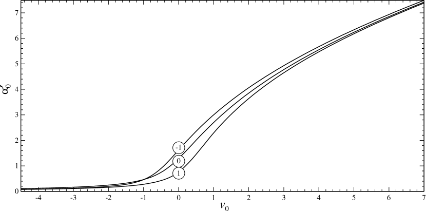
Figure 2: The near-outlet curvature $\alpha_{0}^{\prime}$ of upward-bending curtains vs the excess ejection velocity $v_{0}$. The curves marked by ($\pm 1$) and ($0$) correspond to $\alpha_{0}=\pm\pi/4$ and $\alpha_{0}=0$, respectively.

The mere fact of existence of gravity-defying flows is highly counter-intuitive, but this is not the only paradoxical feature of the solutions found. One would expect faster curtains (those with larger $v_{0}$) to be straighter than their small-$v_{0}$ counterparts – but, in reality, it is the other way around. This tendency is visible in the examples in figure 3, and is quantified in figure 2 (observe the growth of the near-outlet curvature $\alpha_{0}^{\prime}$ with increasing $v_{0}$). Furthermore, sufficiently fast curtains are so curved that they overshoot the vertical direction and come back to it after an inflection point (this pattern is not evident from figure 3, but it is clearly visible in figure 4). It should be emphasized, however, that solutions with large $\alpha_{0}^{\prime}$ may violate the slender-curtain approximation. Recalling how the problem was nondimensionalised, one can show that the applicability condition of the solutions found is $\left|\alpha_{0}^{\prime}\right|\ll\epsilon^{-1}$.

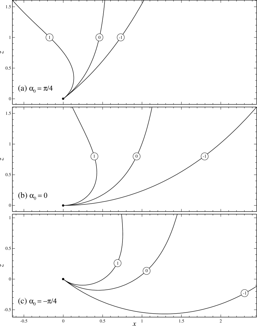
Figure 3: Examples of upward-bending curtains, as described by the boundary-value problem (75)–(78), (81). The values of the ejection angle $\alpha_{0}$ are indicated in the corresponding panels, the values of $v_{0}$ mark the corresponding curves.

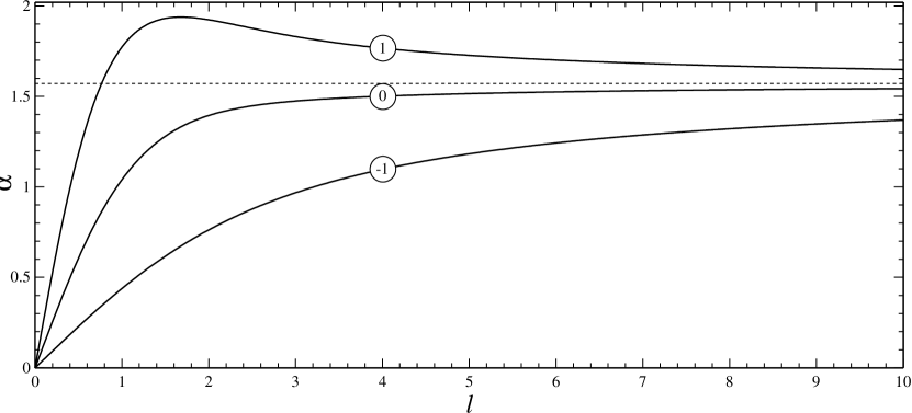
Figure 4: The local angle $\alpha$ between the curtain and the horizontal vs the centreline’s arclength $l$, for the examples shown in figure 3(b) ($\alpha_{0}=0$, the values of $v_{0}$ mark the corresponding curves). Observe that curve (1) overshoots the vertical direction (shown by the dotted line) and comes back to it after an inflection point.

The dependence of UB curtains on the ejection angle $\alpha_{0}$ does not seem to be essential, as the trajectories of curtains with different values of $\alpha_{0}$ are qualitatively similar. Observe also that the curves with different $\alpha_{0}$ in figure 2 are close to each other. One can expect a different behaviour only in the limit $\alpha_{0}\rightarrow-\pi/2$ (nearly vertical curtains), which is not considered here.

(2) As mentioned before, the trajectories of DB curtains can be computed by simply choosing a value of $\alpha_{0}^{\prime}$ and shooting the solution from $l=0$ towards $l\rightarrow\infty$. Numerous examples have been computed via this approach, some of which are shown in figure 5.

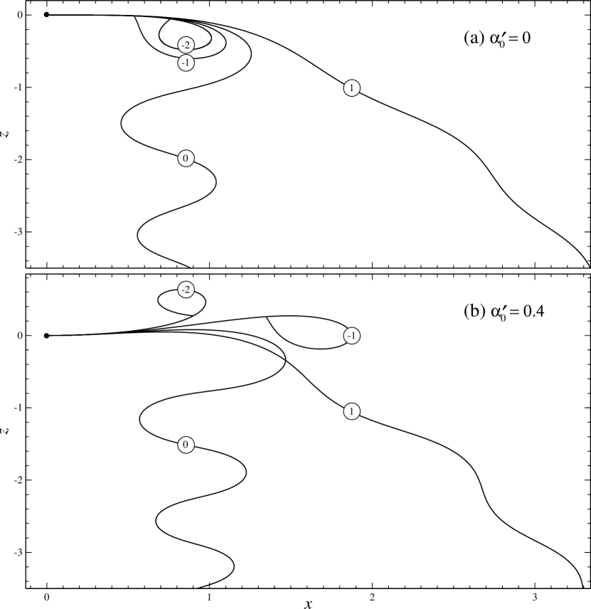
Figure 5: Examples of downward-bending curtains, as described by problem (75)–(78), (79) with $\alpha_{0}=0$. The values of the parameter $\alpha_{0}^{\prime}$ are indicated in the corresponding panels, the values of $v_{0}$ mark the corresponding curves. Panels (a) and (b) correspond to the two horizontal cross-sections of figure 6 labelled “Fig. 5a” and “Fig. 5b”, respectively.

Three features of these examples catch one’s eye. First, DB curtains are wavy (unlike the UB curtains examined above, as well as the DB curtains with $We\not\approx 1$ examined in B19). Second, curtains with a sufficiently negative $v_{0}$ become so wavy that they self-intersect (in figure 5, only the first intersection is shown; after that, the solution is meaningless physically). Third, some of the self-intersecting curtains bend initially upwards (but if their trajectories were extended beyond all intersections, one would see that they turn downwards eventually).

(3) UB and DB curtains can be viewed as different members of the same family of solutions, as illustrated in figure 6.

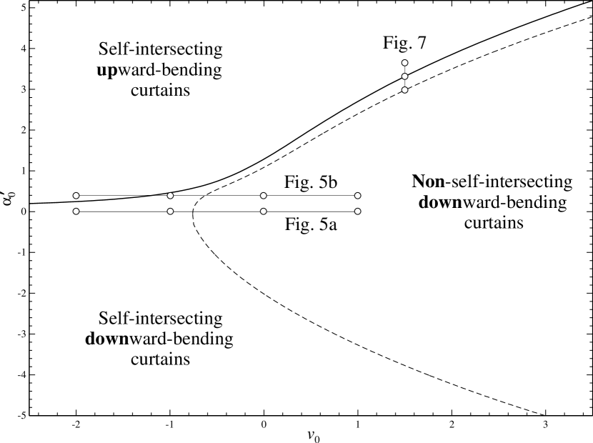
Figure 6: Classification of curtains on the $\left(v_{0},\alpha_{0}^{\prime}\right)$ plane, as described by problem (75)–(78) with $\alpha_{0}=0$. The thick solid curve corresponds to non-self-intersecting upward-bending curtains (it is the same as curve (0) in figure 2). The dashed line bounds the region of self-intersecting curtains. The curtains depicted in figures 5 and 7 correspond to the circles connected by thin solid straight lines.

From now on, self-intersecting curtains will be classified as UB or DB depending on how they behave before the first intersection. Then, the curve corresponding to non-self-intersecting UB solutions should be viewed as a separatrix between self-intersecting UB and DB curtains.

Examples of near-separatrix curtains are shown in figure 7.

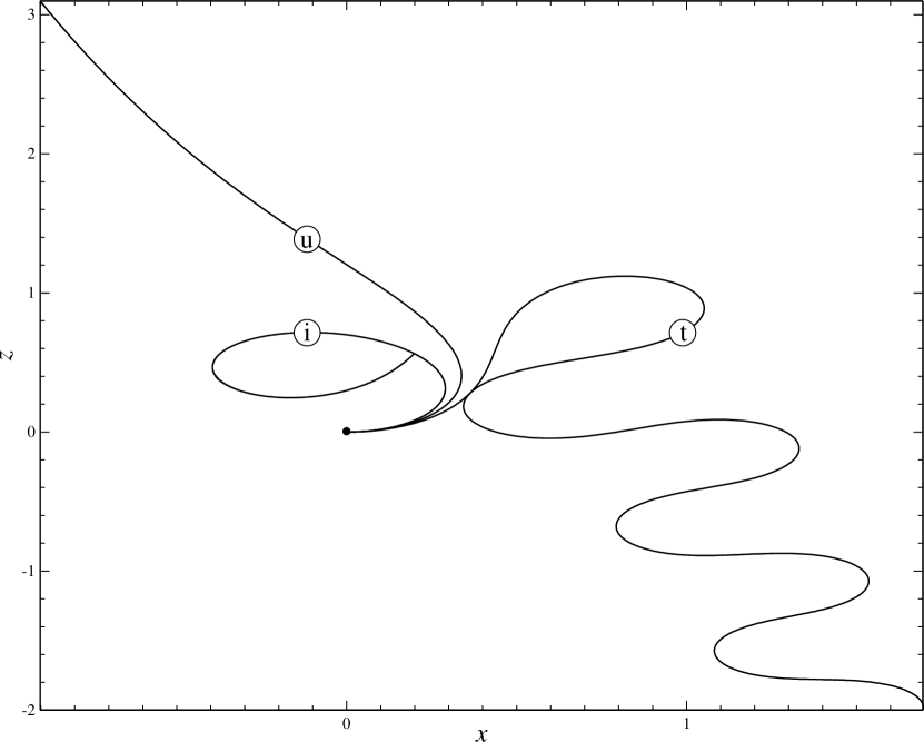
Figure 7: Examples of curtains with $\alpha_{0}=0$ and $v_{0}=1.5$. Curve (u) is the non-intersecting UB curtain ($\alpha_{0}^{\prime}\approx 3.3177$); curve (i) is an example of a self-intersecting UB curtain (with $\alpha_{0}^{\prime}=3.6467$); curve (t) is the self-touching curtain separating self-intersecting and non-self-intersecting DB curtains ($\alpha_{0}^{\prime}\approx 2.9799$). The solutions depicted correspond to the vertical cross-section of figure 6 labelled “Fig. 7”.

4.3 Comparison with B19

(1) In B19, UB curtains could only rise to the height where the fluid velocity vanishes, and so all of the initial reserve of kinetic energy is used up. In the present model, on the other hand, the leading-order nondimensional velocity is unity [see (37)] and, thus, cannot vanish – so the UB curtains formally rise infinitely high. However, it follows from (51) that

$$u^{(2)}\sim-z\qquad\text{as}\qquad z\rightarrow\infty$$

– as a result, once $z$ becomes $\mathcal{O}(\epsilon^{-2})$, the whole expansion breaks down. This is the present model’s equivalent of the limiting height of curtains in B19.

The growth of $u^{(2)}$ with growing $z$ invalidates the large-$z$ results for DB curtains too, but this occurs when they are almost vertical and their evolution is trivial.

(2) One should keep in mind that B19 assumes the characteristic radius of curvature to be $L=H\,Fr$, whereas the present work considers a shorter scale, $L=H\,Fr^{1/3}$. In addition, the present work assumes $We\approx 1$.

Thus, the two sets of results should agree only if the limit $We\rightarrow 1$ is applied to the B19 solutions, whereas the present solutions are subject to

$$\alpha_{0}^{\prime}\ll 1,\qquad v_{0}\gg 1.$$ (85)

These two constraints guarantee that the curtain’s nondimensional curvature is small both near the outlet and globally (as follows from equation (75) with $v_{0}\gg 1$, the solution’s global spatial scale is proportional to $v_{0}$).

(3) According to the present results, UB curtains exist for all $v_{0}$, both positive and negative – whereas B19 found such solutions only in the subcritical case $v_{0}<0$.

The apparent contradiction can be resolved if one recalls that, for UB curtains, $\alpha_{0}^{\prime}$ is a function of $v_{0}$ and $\alpha_{0}$, such that $\alpha_{0}^{\prime}\rightarrow\infty$ as $v_{0}\rightarrow\infty$ (see figure 2). Clearly, such solutions are inconsistent with limit (85), and so it comes as no surprise that supercritical UB curtains have been missed by the asymptotic model of B19.

(4) There is another apparent discrepancy between B19 and the present work: in the former, a single DB curtain was found for given ejection velocity and angle, whereas the latter found a whole family of solutions, differing from each other by their values of $\alpha_{0}^{\prime}$.

To resolve the discrepancy, one should look at the curtains found in the present work under conditions (85) – see figure 8. Observe that the medium-$v_{0}$ curtains with different $\alpha_{0}^{\prime}$ are located much closer together than their small-$v_{0}$ counterparts, and the curtains with the largest value of $v_{0}$ are hardly distinguishable.

Figure 8: Examples of downwards-bending curtains with $\alpha_{0}=0$. The three curves with $v_{0}=2$ are for $\alpha_{0}^{\prime}=\pm 2.5,~{}0$, those with $v_{0}=5$ are for $\alpha_{0}^{\prime}=\pm 1,~{}0$, and those with $v_{0}=12.5$ are for $\alpha_{0}^{\prime}=\pm 0.4,~{}0$.

Thus, in limit (85), curtains with different $\alpha_{0}^{\prime}$ collapse onto the same curve, i.e., the dependence on $\alpha_{0}^{\prime}$ becomes weak – which reconciles the present results with those of B19.

Figure 8 also illustrates the fact that limit (85) makes curtains less wavy, just as they should be according to B19.

5 Physical aspects of the solutions found

(1) Experiments with capillary curtains are difficult to carry out. The problem is that, unless the curtain’s edges are fixed, they tend to retract and the curtain contracts into a circular jet.

There are two ways to fix curtains’ edges: either by walls (e.g. FinnicumWeinsteinRuschak93) or guiding wires (e.g. RocheGrandBrunetLebonLimat06; LhuissierBrunetDorbolo16). Both worked well with vertical curtains – but with oblique ones, they probably would not. Walls imply existence of contact lines which may be pinned and, thus, can prevent the curtain from assuming its natural shape, whereas wires certainly prevent the curtain from assuming it. The best option seems to consist in replacing the curtain with a liquid bell of a large radius (P. Brunet, private communication) which does not have edges.

(2) To come to terms with the counter-intuitive properties of liquid curtains, one should keep in mind that one’s intuition may be misled by one’s everyday experience with jets (those from taps and garden hoses). There is an important difference between the two types of flows: if the Weber number of a jet is order-one, it is highly unstable and breaks down near the outlet by the Plateau–Rayleigh instability, so no-one knows what shape it would have if it were stable. Capillary curtains, on the other hand, are presumably stable – as suggested by experiments with bells (BrunetClanetLimat04; JamesonJenkinsButtonSader10) and vertical curtains (FinnicumWeinsteinRuschak93; RocheGrandBrunetLebonLimat06), as well theoretical studies of the latter (BenilovBarrosObrien16; GirfoglioDerosaCoppolaLuca17).

(3) The most counter-intuitive feature of DB curtains is the non-uniqueness of the solution for a given ejection angle and velocity. Each of the existing solutions represents a sinuous capillary wave, with spatially dependent amplitude and wavenumber – such that the wave’s local phase velocity matches that of the flow. These solutions differ from each other by the wave’s amplitude linked to the parameter $\alpha_{0}^{\prime}$: a larger $\left|\alpha_{0}^{\prime}\right|$ generally corresponds to a stronger wave. Setting $\alpha_{0}^{\prime}=0$, however, does not eliminate the wave entirely (which can be only done by taking the limit $v_{0}\rightarrow\infty$).

The presence in the solution of a wave component with an arbitrary amplitude gives rise to two questions: (A) How are these waves generated? (B) Is there a way to narrow down the family of solutions to the one and only ‘physically meaningful’ solution?

Question (A) can be answered with certainty: capillary waves are generated by the variations of the curtain’s parameters on its way down – simply because a parameter variation in a wave-supporting medium always generates waves.

As for question (B), the steady state of a curtain probably depends on how it was created – or, more generally, on the prior evolution.

One can verify or refute this hypothesis by creating a DB curtain – waiting until it becomes steady – then altering (for a brief period of time) the ejection angle and/or velocity. Once those have regained their original values, will the curtain regain its original shape? To a degree of certainty, this question can be answered through a gedanken experiment – by solving numerically or asymptotically the full (evolutionary) version of problem (33)–(36) with time-dependent $\alpha_{0}(t)$ and $v_{0}(t)$.

(4) The simulation described above may also show how to create a UB curtain experimentally.

Consider a pair of values $\left(\alpha_{0},v_{0}\right)$ corresponding to a non-self-intersecting DB curtain – one of those that do not contradict our intuition. It corresponds to a point in the right-middle part of figure 6, which also shows that the UB curtain with the same pair $\left(\alpha_{0},v_{0}\right)$ has a larger near-outlet curvature $\alpha_{0}^{\prime}$.

Thus, one should be able to create a UB curtain by making a non-self-intersecting DB curtain increase its $\alpha_{0}^{\prime}$.

This cannot be done directly, as $\alpha_{0}^{\prime}$ is not controlled in an experiment. One can, however, alter $\alpha_{0}(t)$ and/or $v_{0}(t)$ in such a way that the final steady state has a greater $\alpha_{0}^{\prime}$ than the initial one.

Indeed, let the injection velocity $v_{0}$ be constant, while the injection angle $\alpha_{0}(t)$ is slowly increased and then abruptly decreased – as one does when cracking a whip. The near-outlet part of the curtain has to adjust to the change of the injection angle, whereas its main bulk – due to its inertia – will lag behind; as a result, $\alpha_{0}^{\prime}$ should grow. If it ends up near the value corresponding to the UB curtain, the resulting steady state should also be close to the UB curtain.

This approach, however, is unlikely to work for strongly subcritical UB curtains, i.e., those with $v_{0}\ll-1$.

To create one of such, a non-self-intersecting DB curtain is needed to start from, but such do not exist in this part of the parameter space (see figure 6). Computations show that solutions there are highly sensitive to small variations of the parameters involved, and that a randomly chosen solution is likely to involve the first self-intersection very close to the outlet. A strongly subcritical curtain can be guaranteed to have a reasonably long non-self-intersecting segment only if $\alpha_{0}^{\prime}$ is close to that of the UB curtain with the same $\left(\alpha_{0},v_{0}\right)$ – but creating such is as difficult as the UB curtain itself.

(5) The range of physically meaningful solutions (for both DB and UB curtains ) is likely to narrow if a stability study is carried out.

Still, one should not expect that a single solution will emerge as stable for each $\left(\alpha_{0},v_{0}\right)$. Indeed, stable flows are generally either nonexistent or occupy a finite-size region in the problem’s parameter space. In the present case, this means that, for some $\left(\alpha_{0},v_{0}\right)$, there may not be any stable solutions at all – and for the others, there are infinitely many solutions, corresponding to a finite-length interval of $\alpha_{0}^{\prime}$.

One can conjecture that unstable curtains are those with high curvature, where the centrifugal force is too strong to be contained by surface tension. If this is indeed so, all strongly supercritical ($v_{0}\gg 1$) UB curtains are unstable (because their near-outlet curvature $\alpha_{0}^{\prime}$ is large – see figure 2).

It should also be mentioned that a sufficiently high curvature invalidates the slender-curtain approximation underlying all of the results obtained.

In view of comments (4)–(5), one should expect UB curtains to be observable only for moderate $v_{0}$ (or, physically, if $We\approx 1$).

6 Concluding remarks

The present work should suffice as a proof concept, but an accurate description of upward-bending curtains should be based on a more comprehensive model.

Firstly, viscosity should be taken into account. This task cannot be done in a single step, as two different regimes will have to be examined. Indeed, let $\nu$ be the liquid’s kinematic viscosity. In B19, its importance was characterised by the nondimensional parameter

$$\mu=\frac{\nu u_{0}}{gH^{2}},$$

and preliminary estimates show that, if

$$\mu\epsilon^{2}\lesssim 1,$$

viscous forces are comparable to those of inertia and surface tension. In this case, one should expect the dynamics of curtains with $We\approx 1$ to be governed by an incremental modification of equation (33). A stronger viscosity, however, should dominate the flow and, thus, significantly change the model.

Secondly, one should extend the present model to sheared flows, as this is the state in which curtains emerge from the outlet. One should still keep in mind that the transitional region where a sheared (say, Poiseuille) flow turns into a plug flow can be very small; for jets, for example, the boundary velocity reaches 50% of its maximum value after a distance of only $l\approx 0.04\,H\,Re$ (see Goren66; Sevilla11, figure 2b). If this applies to liquid curtains as well, the initial shear would have little impact on the global dynamics.

Thirdly, one should examine the stability of steady curtains. Since viscosity is likely to have a significant stabilising effect, stability study should be carried out only after this effect has been incorporated into the model.

Acknowledgments

The author is grateful to Andrew Fowler for a comment which turned out to be crucial for solving this problem.

Declaration of interests

The author reports no conflict of interests.

Appendix A The next-to-leading order of the boundary-layer solution

Observe that, under the condition $\alpha_{0}^{\prime\prime}=0$, the leading-order solution (70)–(72) for the cross-stream velocity amounts to

$$u_{\tau}^{(0)}=0.$$ (86)

Substituting this into the boundary-value problem (67)–(69), one can readily deduce expressions for the rest of the leading-order unknowns,

$$u_{\tau}^{(0)}=0,\qquad p^{(1)}=-\tau^{2}\alpha_{0}^{\prime 2},\qquad\tau_{\pm}^{(2)}=0.$$ (87)

Next, substitute series (66) into the full equations (61)–(65), take into account (86)–(87) and, thus, obtain the next-to-leading-order equations (the subscript _b omitted),

$$\dfrac{\partial u_{l}^{(3)}}{\partial l}+\dfrac{\partial p^{(2)}}{\partial l}=-\sin\alpha_{0},$$

$$\dfrac{\partial u_{\tau}^{(1)}}{\partial l}+2u_{0}\alpha_{0}^{\prime}+\dfrac{\tau^{2}}{2}\left(8\alpha_{0}^{\prime 3}+\alpha_{0}^{\prime\prime\prime}\right)+\dfrac{l^{2}}{2}\alpha_{0}^{\prime\prime\prime}+\dfrac{\partial p^{(2)}}{\partial\tau}=-\cos\alpha_{0},$$

$$\dfrac{\partial}{\partial l}\left(u_{l}^{(3)}+\tau\alpha_{0}^{\prime}u_{0}+\dfrac{\tau l^{2}}{2}\alpha_{0}^{\prime\prime\prime}\right)+\dfrac{\partial u_{\tau}^{(1)}}{\partial\tau}=0,$$

$$\dfrac{\partial\tau_{\pm}^{(3)}}{\partial l}-u_{\tau}^{(1)}=0,\qquad p^{(2)}=\mp\dfrac{\partial^{2}\tau_{\pm}^{(3)}}{\partial l^{2}}\mp\frac{1}{2}\left(3\alpha_{0}^{\prime 3}+\alpha_{0}^{\prime\prime\prime}+l^{2}\alpha_{0}^{\prime\prime\prime}\right)\qquad\text{if}\qquad\tau=\pm 1,$$

$$u_{l}^{(3)}=0,\qquad u_{\tau}^{(1)}=0,\qquad\tau_{\pm}^{(3)}=0\qquad\text{if}\qquad l=0.$$

One can eliminate from this problem all the unknowns except $\hat{u}_{\tau}^{(1)}$ and thus obtain

$$\frac{\partial^{2}u_{\tau}^{(1)}}{\partial\tau^{2}}+2l\alpha_{0}^{\prime\prime\prime}+\frac{\partial^{2}u_{\tau}^{(1)}}{\partial l^{2}}=0,$$ (88)

$$\frac{\partial u_{\tau}^{(1)}}{\partial\tau}-\sin\alpha_{0}=\pm\dfrac{\partial^{2}u_{\tau}^{(1)}}{\partial\tau^{2}}\qquad\text{if}\qquad\tau=\pm 1,$$ (89)

$$u_{\tau}^{(1)}=0\qquad\text{if}\qquad l=0.$$ (90)

It is convenient to introduce $\hat{u}_{\tau}^{(1)}$ such that

$$u_{\tau}^{(1)}=\left(1-\tau^{2}\right)l\alpha_{0}^{\prime\prime\prime}+\tau\sin\alpha_{0}+l\frac{\partial\alpha_{0}}{\partial t}+\hat{u}_{\tau}^{(1)}.$$ (91)

In terms of the new unknown, (88)–(90) become

$$\frac{\partial^{2}\hat{u}_{\tau}^{(1)}}{\partial\tau^{2}}+\frac{\partial^{2}\hat{u}_{\tau}^{(1)}}{\partial l^{2}}=0,$$ (92)

$$\frac{\partial\hat{u}_{\tau}^{(1)}}{\partial\tau}=\pm\dfrac{\partial^{2}\hat{u}_{\tau}^{(1)}}{\partial\tau^{2}}\qquad\text{if}\qquad\tau=\pm 1,$$ (93)

$$\hat{u}_{\tau}^{(1)}=-\tau\sin\alpha_{0}\qquad\text{if}\qquad l=0.$$ (94)

This boundary-value problem can be solved using the Fourier sine transformation, but the Fourier transform of $\hat{u}_{\tau}^{(1)}$ would be singular, and it is not clear how the singularity should be regularised. Its physical meaning, however, is clear: it describes a semi-infinite wave generated in the boundary layer and radiated into the outer region. Since the structure and wavenumber of this wave are easy to find, one can leave the wave’s amplitude arbitrary and ‘subtract’ the wave solution from $\hat{u}_{\tau}^{(1)}$. Once the Fourier transform of the modified solution is found, one can require it to be non-singular and thus find the (so far undetermined) amplitude.

Following the above plan, introduce $U(l,\tau,t)$ such that

$$\hat{u}_{\tau}^{(1)}=U+B^{(1)}\cos k_{\ast}l\,\sinh k_{\ast}\tau+A^{(1)}\sin k_{\ast}l\,\sinh k_{\ast}\tau,$$ (95)

where $k_{\ast}$ is determined by (71), $B^{(1)}$ is the amplitude of the wave radiated towards infinity, and $A^{(1)}$ is the amplitude of the wave coming from infinity – bouncing off the outlet – and going back to infinity. Substituting (95) into (92)–(94) and taking into account (71) to simplify the boundary condition (93), one obtains

$$\frac{\partial^{2}U}{\partial\tau^{2}}+\frac{\partial^{2}U}{\partial l^{2}}=0,$$ (96)

$$\frac{\partial U}{\partial\tau}=\pm\dfrac{\partial^{2}U}{\partial\tau^{2}}\qquad\text{if}\qquad\tau=\pm 1,$$ (97)

$$U=-\tau\sin\alpha_{0}-B^{(1)}\sinh k_{\ast}\tau\qquad\text{if}\qquad l=0.$$ (98)

Observe that $A^{(1)}$ remains undetermined, just like its previous-order counterpart $A^{(0)}$ in expression (70).

Rewriting (96)–(98) in terms of the Fourier transform

$$\tilde{U}(k,\tau,t)=\int_{0}^{\infty}U(l,\tau,t)\sin kl\,\mathrm{d}l,$$

one obtains

$$\frac{\partial^{2}\tilde{U}}{\partial\tau^{2}}-k\left(\tau\sin\alpha_{0}+B^{(1)}\sinh k_{\ast}\tau\right)-k^{2}\tilde{U}=0,$$

$$\frac{\partial\tilde{U}}{\partial\tau}=\pm\dfrac{\partial^{2}U}{\partial\tau^{2}}\qquad\text{if}\qquad\tau=\pm 1.$$

This boundary-value problem can be readily solved,

$$\tilde{U}=\frac{\sinh k\tau}{\cosh k-k\sinh k}\left[\frac{\sin\alpha_{0}}{k^{2}}+\frac{B^{(1)}k\left(\cosh k_{\ast}-k\sinh k_{\ast}\right)}{k^{2}-k_{\ast}^{2}}\right]\\ -\frac{\tau\sin\alpha_{0}}{k}-\frac{kB^{(1)}\sinh k_{\ast}\tau}{k^{2}-k_{\ast}^{2}}.$$ (99)

Observe that (99) is not singular at $k=k_{\ast}$ only if

$$B^{(1)}=\frac{2\sin\alpha_{0}}{k_{\ast}^{2}\sinh k_{\ast}}.$$ (100)

Together with the expression for the inverse Fourier transform,

$$U(l,\tau,t)=\frac{2}{\pi}\int_{0}^{\infty}\tilde{U}(k,\tau,t)\sin kl\,\mathrm{d}l,$$

formulae (99)–(100) complete the solution of problem (92)–(94).

It can be shown that the non-oscillating part of the boundary-layer solution found matches the outer solution – but the wave part [the second and third terms in (95)] implies the inclusion of similar terms in the outer solution. This has not been done, as such (small and fast-oscillating) component would affect the global dynamics only when it appears in quadratic terms – just as the fast wave component in the Davey–Stewartson system (DaveyStewartson74). In the present problem such terms come up in the fourth order of the perturbation expansion – whereas the leading-order dynamics [equation (75)] emerges in the third order.

Furthermore, if viscosity is introduced, the radiated wave is confined to the boundary layer and, thus, its effect on the global dynamics is exponentially weak.

Finally, observe that $u_{\tau}^{(1)}$ is an odd function of $\tau$, which means that it describes varicose capillary waves. Given that $u_{\tau}^{(0)}$ is zero, this conclusion applies to the whole boundary-layer solution.

Appendix B Numerical solution of problem (75)–(78), (81)

As argued in §4.1, the exponentially growing term in asymptotics (82)–(84) has to be eliminated by setting $C_{2}=0$, whereas the term involving $\tilde{\alpha}_{3}$ decays faster than $1/l^{n}$ for any $n>0$. Thus, the large-$l$ asymptotics of the solution of the full (non-linearised) problem can be sought in the form of a power series in $1/l$.

Before doing this, however, it is convenient to introduce

$$\Delta=z-l,$$

then define

$$\Delta_{\infty}=\lim\limits_{l\rightarrow\infty}\Delta,$$

and rewrite (75) and the second equation of (76) in the form

$$\left.\begin{array}[]{l}\dfrac{\mathrm{d}\alpha}{\mathrm{d}l}=\alpha^{\prime},\vskip 6.0pt plus 2.0pt minus 2.0pt\\ \dfrac{\mathrm{d}\alpha^{\prime}}{\mathrm{d}l}=\alpha^{\prime\prime},\vskip 6.0pt plus 2.0pt minus 2.0pt\\ \dfrac{\mathrm{d}\alpha^{\prime\prime}}{\mathrm{d}l}=\alpha^{\prime}\left[3\left(\tilde{l}+\Delta-\Delta_{\infty}\right)-\dfrac{1}{2}\alpha^{\prime 2}\right]-3\cos\alpha,\vskip 6.0pt plus 2.0pt minus 2.0pt\\ \dfrac{\mathrm{d}\Delta}{\mathrm{d}l}=\sin\alpha-1,\end{array}\right\}$$ (101)

where $\tilde{l}$ is given by (84). The boundary conditions (77) and the second condition of (78), in turn, take the form

$$\alpha(0)=\alpha_{0}\qquad\alpha^{\prime}(0)=\alpha_{0}^{\prime},\qquad\alpha^{\prime\prime}(0)=0\qquad\Delta(0)=0.$$ (102)

At infinity, let

$$\left.\begin{array}[]{l}\alpha=\frac{1}{2}\pi+\alpha_{1}\tilde{l}^{-1}+\alpha_{2}\tilde{l}^{-2}+\alpha_{3}\tilde{l}^{-3}+\alpha_{4}\tilde{l}^{-4}+\mathcal{O}(\tilde{l}^{-5})\vskip 6.0pt plus 2.0pt minus 2.0pt\\ \Delta=\Delta_{\infty}+\Delta_{1}\tilde{l}^{-1}+\Delta_{2}\tilde{l}^{-2}+\Delta_{3}\tilde{l}^{-3}+\Delta_{4}\tilde{l}^{-4}+\mathcal{O}(\tilde{l}^{-5})\end{array}\right\}\qquad\text{as}\qquad l\rightarrow\infty.$$ (103)

Substituting asymptotics (103) into equations (101), one can relate the coefficients in (103) to one of them – say, $\alpha_{1}$ – and thus obtain

$$\left.\begin{array}[]{c}\alpha_{2}=0,\qquad\alpha_{3}=-\frac{1}{3}\alpha_{1}^{3},\qquad\alpha_{4}=\frac{2}{3}\alpha_{1},\vskip 6.0pt plus 2.0pt minus 2.0pt\\ \Delta_{1}=\frac{1}{2}\alpha_{1}^{2},\qquad\Delta_{2}=0,\qquad\Delta_{3}=-\frac{1}{8}\alpha_{1}^{4},\qquad\Delta_{4}=\frac{1}{6}\alpha_{1}^{2}.\end{array}\right\}$$ (104)

Note that asymptotics (103)–(104) involve three undetermined parameters: $\Delta_{\infty}$, $\alpha_{1}$, and $\alpha_{0}^{\prime}$ [the last one is ‘hidden’ in $\tilde{l}$, and also appears in equations (101) and boundary conditions (102)].

To solve equations (101) subject to the boundary conditions (102)–(104), one should pick a large $l_{\infty}$ and require that three of the four unknowns $\left(\alpha,\alpha^{\prime},\alpha^{\prime\prime},\Delta\right)$ coincide at $l=l_{\infty}$ with the values predicted by the asymptotics (103)–(104). This way, the solution will be fixed together with the parameters $\Delta_{\infty}$, $\alpha_{1}$, and $\alpha_{0}^{\prime}$.

This approach was realised twice: using the shooting method and the MATLAB function BVP4c (based on the three-stage Lobatto IIIa formula – see KierzenkaShampine01). The former was found to work only if $l_{\infty}\lesssim 7$, and so was used only to validate the latter. In either case, the results were independent of which three of the four unknowns are fixed at $l=l_{\infty}$.