Simulating and Classifying Behavior in Adversarial Environments Based on Action-State Traces: An Application to Money Laundering

Abstract

Many business applications involve adversarial relationships in which both sides adapt their strategies to optimize their opposing benefits. One of the key characteristics of these applications is the wide range of strategies that an adversary may choose as they adapt their strategy dynamically to sustain benefits and evade authorities. In this paper, we present a novel way of approaching these types of applications, in particular in the context of Anti-Money Laundering. We provide a mechanism through which diverse, realistic and new unobserved behavior may be generated to discover potential unobserved adversarial actions to enable organizations to preemptively mitigate these risks. In this regard, we make three main contributions. (a) Propose a novel behavior-based model as opposed to individual transactions-based models currently used by financial institutions. We introduce behavior traces as enriched relational representation to represent observed human behavior. (b) A modelling approach that observes these traces and is able to accurately infer the goals of actors by classifying the behavior into money laundering or standard behavior despite significant unobserved activity. And (c) a synthetic behavior simulator that can generate new previously unseen traces. The simulator incorporates a high level of flexibility in the behavioral parameters so that we can challenge the detection algorithm. Finally, we provide experimental results that show that the learning module (automated investigator) that has only partial observability can still successfully infer the type of behavior, and thus the simulated goals, followed by customers based on traces - a key aspiration for many applications today.

1 Introduction

Adversarial settings are common in many business domains, where both sides adapt their strategies over time. For example, money laundering vs Anti-Money Laundering (AML), or those in fraud, and cyber-crime. If we take AML, a key characteristic is the wide range of strategies that are available to a money launderer, who may come up with completely novel, previously unseen strategies to evade authorities. At present, models available to investigators involve playing catch-up. Investigators may happen to detect a new typology used by a money launderer and may make recommendations to put in new controls for the novel typology detected. Subsequently, the organization may adjust their models to counter the newly observed strategy to allow its detection going forward. However, significant delay and crime might have passed through by the time new controls are put in place. Money launderers, fraudsters, or other bad actors often remove and obscure the funds (benefits) from the networks to nullify their risk of any future cease of funds, in case of any retrospective action by authorities. Hence, timely detection of previously unseen typologies is of utmost importance.

In this paper, we focus on AML. As defined by Senator et al. (?), “Money laundering is a complex process of placing the profit …from illicit activity into the legitimate financial system, with the intent of obscuring the source, ownership, or use of the funds.” Over time, financial institutions have been mandated by law enforcement agencies to improve their processes to detect suspicious activity and raise the corresponding Suspicious Activity Reports (SARs). A typical prevalent AML model starts by observing transactions, public media, or a referral, and generates alerts [Isa et al., 2015]. Then, alerts are investigated by humans who decide whether they need to report a SAR to law enforcement for the alert. Since there is a bias towards being conservative and raising alerts at the detection of any suspicious behavior, many alerts are generated and the manual effort put into investigations is enormous [Takáts, 2011]. However, despite all these efforts, most of the money laundering activities are not noticed in time. Europol estimates that less than 1% of money originating from criminal activities is recovered in Europe.

In order to provide efficient AI tools to help human investigators and law enforcement, any investigation needs to provide rationale for its decisions, as filing a SAR. Rationale usually constitutes of gathering all “applicable” set of evidences via a sequence of steps and a final assessment of all evidences. Mostly, applicable evidences deal with inferring subject’s goals. Therefore, in order to be used in practice, the output of any AI-based system that tackles this task should explicitly mention the goals the suspects were pursuing, as well as the actions the subjects of interest carried out and the evidences that led to that conclusion.

Previous work on automating AML has defined sets of rules to detect particular behaviors [Rajput et al., 2014, Senator et al., 1995], or applied machine learning to transactions or social networks [Chen et al., 2018, Fronzetti Colladon and Remondi, 2017]. Most of these recent works use neural network (NN) based approaches [Weber et al., 2018, Schlichtkrull et al., 2018]. These approaches have shown exceptional performance for many tasks including image classification or natural language processing. But, given their current way of handling explanations, they are not yet a viable solution from a practical perspective. Instead, symbolic approaches are clearly much better suited for tasks requiring explanations. Other approaches used a variety of AI techniques to solve the AML classification task, such as SVMs [Kingdon, 2004], Dynamic Bayesian Networks and clustering [Raza and Haider, 2011], RBF neural networks [Lin-Tao et al., 2008], fuzzy logic [Chen and Mathe, 2011], association rules and frequent set analysis [Luo, 2014], clustering [Larik and Haider, 2011] or decision trees [Wang and Yang, 2008]. In general, most of these papers and others published on applying machine learning (or other AI techniques) to AML, do not include comparison with other works, and use their own simulators and data. We include in this paper a comparison of our relational learning technique against a decision tree. The AML task can also be posed as anomalies or outliers detection [Chandola et al., 2010, Gupta et al., 2013] where the techniques and representation formalisms are also based on attribute-value.

In this paper, we assume there is a rationale for the behavior of agents (customers) when taking actions in the environment that is partially observable by a financial institution. This behavior depends on some hidden human goals and the states they encounter while taking actions to achieve those goals. We also assume goals, states and actions can be represented using a form of high-level representation formalism, such as predicate logic. These assumptions are in line with the need to file rationale for each SAR. The evidences compiled in SARs correspond to descriptions of actions (activities) taken by suspicious persons (e.g. several cash deposits) and the corresponding states (e.g. network of people and companies). While all this knowledge could potentially be represented in the attribute-value representation used by most other AI techniques applied to AML, usually we have to constrain the size of the representation, require some extensive domain-dependent feature engineering or lose representation power [Dzeroski and Lavrac, 2010].

Given those assumptions, we can pose the problem of AML as a relational classification task [Dzeroski and Lavrac, 2010]. It takes as input a trace of human behavior corresponding to the execution of observable actions by the financial institution and the corresponding observable components of states. It generates as output a decision of whether that trace corresponds to money laundering or not. We train our learning system with previous traces of known behavior (both money laundering or not), which can be trivially extracted from current information systems of financial institutions in a relational format. We name our learning system cabbot for Classification of Agents’ Behavior Based on Observation Traces. Process mining is a related field whose goals include identifying processes from traces [van der Aalst, 2016]. However, most work on process mining assumes actions are represented as labels (no parameters), and there is very little reasoning on states and goals as logical formulae.

We present as main contributions of this research: a new enhanced model of human behavior in the context of financial institutions based on states and actions; a learning technique that can classify in agents’ (or behavior) types based on observation traces; and a simulator of agents’ behavior based on dynamic goal generation, planning and execution. Since most available datasets on AML correspond to only transactions data, we have built a simulator that generates realistic traces of these kinds of behavior and incorporates a rich representation of actions and states.

2 States and Actions Traces

We assume agents’ rational behavior to be based on the concepts of goals, states and actions. In order to establish a common representation language, we will use a form of predicate logic to represent the information that an agent (such as a financial institution), $F$, can observe from the behavior of another agent (e.g. customer), $C$. States will be represented as sets of literals, where literals can be predicates or functions. Predicates have a name and a list of arguments (e.g. account-owner(c1,acc1)). Functions represent numeric variables and are composed of a name, its arguments and the value (e.g. balance(acc1)=12020). As in the real world, part of the state will be observable by $F$ and another part will not be observable. For instance, the owner of an account will be observable by a financial institution, while the fact that someone is trying to launder money will not be observable.

2.1 Representation of States and Goals

Tables 1 and 2 lists the key predicates and functions we have defined. They can refer to four categories of information: transaction-based; relationship-based, related to the network of people or companies connected to each customer; both kinds, transaction and network; or to the bank, but not related to network or transactions. The tables also represent their observability.

Predicate	Observable	Type
money-laundering	no
money-laundered	no
has-dirty-money	no
criminal	no
banned-country	yes	network
account-owner	yes	network
account-country	yes	network
member-of	yes	network
bill-due	yes	network
owes-money	no
employed	yes	network
works-for	yes	network
has-company	yes	network
transaction-origin	yes	transactions
transaction-destination	yes	transactions
received-payroll	yes	both
has-card	yes	bank
enjoyed-service	no
provides-service	no
owns	no

Table 1: List of predicates, their observability and the type of information they refer to in case they are observable.

Function	Observable	Type
balance	yes	both
transaction-amount	yes	transactions
dirty-money	no
criminal-income	no
working-day	no
days-without-pay	no
salary	no
price	no
owed-money	no

Table 2: List of functions, their observability and the type of information they refer to in case they are observable.

2.2 Representation of Actions

Table 3 lists the key actions we have defined, together with the same data as in the case of predicates. We duplicate some of these actions, since they can be used by standard customers or criminals. $F$ will observe criminals’ actions as their corresponding standard ones. For instance, integration-cash-out represents a withdrawal following money laundering, but $F$ will observe it as a cash-out action.

Action	Observable	Type
create-company	no
associate	no
create-account	yes	network
set-ownership-account	yes	network
perform-criminal-action	no
finish-money-laundering	no
takes-job	no
work	no
payroll	yes	both
quick-deposit	yes	transactions
placement-cash-in	yes	transactions
digital-deposit	yes	transactions
placement-digital	yes	transactions
buy-digital	no
cash-out	yes	transactions
integration-cash-out	yes	transactions
pay-bill	yes	both
create-bill	no
integration-pay-bill	yes	both
move-funds	yes	transactions
move-funds-internationally	yes	transactions
move-funds-self	yes	transactions
layering	no
quick-payment	yes	transactions
buy-direct	yes	transactions
placement-buy-direct	yes	transactions
enjoy-service	yes	transactions
placement-enjoyed-service	yes	transactions

Table 3: List of actions, their observability and the type of information they refer to in case they are observable.

2.3 Traces of Behavior

The learning system takes as input traces of observable behavior. A trace $t_{C}$ is a sequence of states and actions executed by $C$ in those states: $t_{C}=(s_{0},a_{1},s_{1},a_{2},s_{2},\ldots,s_{n-1},a_{n},s_{n})$, where $s_{i}$ is a state and $a_{i}$ is an action name and its parameters. States and actions correspond to the observable predicates and actions from the viewpoint of $F$. We will call $T_{C}=\{t_{C}\}$ the set of traces observed from $C$.

We assume there is nothing in the observable state that directly identifies one or the other type of behavior. There is also no difference on the observable actions between those that can be executed by one or the other type of $C$.

3 Learning to Classify Behavior

$F$’s task consists of learning to classify among the different types of $C$ (behaviors).

3.1 Learning Task

The learning task can be defined as follows. Given: $N$ classes of behavior, ({good, bad} in our current application); and a set of labeled observed traces, $T_{C_{i}},\forall C_{i}\in\{{\mbox{g}ood,bad}\}$ Obtain: a classifier that takes as input a new (partial) trace $t$ (with unknown class) and outputs the predicted class.

A characteristic of this learning task is that it works on unbounded size of the learning examples. Traces can be arbitrarily large. Also, states within the trace and action descriptions can be arbitrarily large (both in the number of different action schemas, and in the number of grounded actions). Using fixed-sized input learning techniques can be difficult in these cases and some assumptions are made to handle that characteristic. Therefore, we will consider only relational learning techniques, and, in particular, relational instance-based approaches.

We use relational $k$NN (ribl) to classify a new trace according to the $k$ traces with minimum distance, and then computing the mode of those traces’ classes. Since the classifier takes a trace as input, cabbot also allows for on-line classification with the current trace up to a given execution step. A nice property of $k$NN is that we can explain how a behavior was classified by pointing out the closest previous cases and which are the most similar components (actions and states) of the closest traces.

3.2 Distance Functions between Traces

The key parameter of the relational learning techniques we will use is the distance between two traces, $d:T\times T\rightarrow\mathbb{R}$. Similarity functions have been extensively studied [Ontañón, 2020]. We have defined four distance metrics that can deal with state-action traces: actions; state differences; n-grams; and relational.

Distance based on Actions. A simple, yet effective, distance function consists of using the inverse of the Jaccard similarity function [Jaccard, 1901] as:

$d_{a}(t_{1},t_{2})=1-\frac{|an(t_{1})\cap an(t_{2})|}{|an(t_{1})\cup an(t_{2})|}$

where $an(t_{i})$ is the set of actions names in $t_{i}$. This distance is based on the ratio of common action names in both traces to the total number of different action names in both traces.

Distance based on State Differences. Given two consecutive states $s_{1}$ and $s_{2}$ in a trace, we define their associated difference or delta as $\delta_{s_{i},s_{i+1}}=s_{i+1}\setminus s_{i}$. These deltas represent the new literals in the state after applying the action. We can compute a distance between the sets of deltas on each trace by using the Jaccard similarity function as before.

$d_{\Delta}(t_{1},t_{2})=1-\frac{|\Delta(t_{1})\cap\Delta(t_{2})|}{|\Delta(t_{1})\cup\Delta(t_{2})|}$

where $\Delta(t_{i})$ is the set of deltas of a trace $t_{i}$. Again, we only use the predicate and function names.

Distance based on $n$-grams. The two previous distances only consider actions and deltas as sets. If we want to improve the distance metric, we can use a frequency-based approach (equivalent to an $n$-grams analysis with $n=1$). Each trace is represented by a vector. Each position of the vector contains the number of times an observable action appears in the trace. The distance between two traces, $d_{g}$, is defined as the squared Euclidean distance of the vectors representing the traces. As before, a new trace is classified as the class of the training trace with the minimum distance to the new trace.

Relational-based Distance. Instead of using only counts, the distance function can also consider action and state changes as relational formulae and use more powerful relational distance metrics. We define a version of the ribl relational distance function [Emde and Wettschereck, 1996] adapted to our representation of traces, $d_{r}$. We modify it given the different semantics of the elements of the traces with respect to generic ribl representation of examples. Given two traces, we first normalize the traces by substitution of the constants’ names by an index of the first time they appeared within a trace. For instance, given the following action and state:

$\langle$	create-account(customer-234,acc-345),
	{	acc-owner(customer-234,acc-345)
	balance(acc-345)=2000} $\rangle$

the normalization process would convert the trace to:

$\langle$	create-account(i1,i2),
	{acc-owner(i1,i2),balance(i2)=2000} $\rangle$

This process allows the distance metric to partially remove the issue related to using different constant names in the traces. The distance $d_{r}$ is then computed as:

$$d_{r}(t_{1},t_{2})=\frac{1}{2}(d_{ra}(t_{1},t_{2})+d_{r\Delta}(t_{1},t_{2}))$$

i.e. as the average of the sum of $d_{ra}$ (distance between the actions of the two traces) and $d_{r\Delta}$ (distance between the deltas of both traces). $d_{ra}$ is computed as:

$$d_{ra}(t_{1},t_{2})=\frac{1}{Z}\sum_{a_{i}\in a(t_{1})}\min_{a_{j}\in a(t_{2})}d_{f}(a_{i},a_{j})$$

where $a(t_{i})$ is the set of ground actions in $t_{i}$, $d_{f}$ is the distance between two relational formulae and $Z$ is a normalization factor ($Z=\max\{|a(t_{1})|,|a(t_{2})|\}$). We normalize by using the length of the longest set of actions to obtain a value that does not depend on the number of actions on each set, so distances are always between 0 and 1. $d_{f}$ is 1 if the names of $a_{i}$ and $a_{j}$ differ. Otherwise, it is computed as:

$d_{f}(a_{i},a_{j})=0.5-0.5\frac{1}{|\mbox{arg}(a_{i})|}d_{\mbox{arg}}(a_{i},a_{j})$

where $d_{\mbox{arg}}(a_{i},a_{j})$ is the sum of the distances between the arguments in the same positions in both actions. Each distance will be 0 if they are the same constant and 1 otherwise. Again, we normalize the values for distances. Also, when two grounded actions have the same action name, we set a distance of at most 0.5. For instance, if we have two literals $l_{1}=$create-account(i1,i2) and $l_{2}=$create-account(i3,i2),

$d_{f}(l_{1},l_{2})=0.5-0.5\frac{1}{2}(1+0)=0.25$.

As a reminder, each trace contains a sequence of sets of literals that correspond to the delta of two states. Therefore, $d_{r\Delta}$ is computed as the distance of two sets of deltas of literals ($\Delta(t_{1})$ and $\Delta(t_{2})$). We use a similar way to compute it as in the previous formulas:

$d_{r\Delta}(t_{1},t_{2})=\frac{1}{Z_{\Delta}}\sum_{\delta_{1}\in\Delta(t_{1})}\min_{\delta_{2}\in\Delta(t_{2})}d_{r\delta}(\delta_{1},\delta_{2})$

where $Z_{\Delta}=\max\{|\Delta(t_{1})|,|\Delta(t_{2})|\}$, and $d_{r\delta}$:

$$d_{r\delta}(\delta_{1},\delta_{2})=\frac{1}{\max\{|\delta_{1}|,|\delta_{2})|\}}\sum_{l_{i}\in\delta_{1}}\min_{l_{j}\in\delta_{2}}d_{f^{\prime}}(l_{i},l_{j})$$

$d_{f^{\prime}}(l_{i},l_{j})=d_{f}(l_{i},l_{j})$ when the literals correspond to predicates. We use $d_{f}$ since actions and literals in the state ($l_{j},l_{j}$) share the same format (a name and some arguments). However, when they correspond to functions, since functions have numerical values, we have to use a different function $d_{n}$. In this case, each $l_{i}$ will have the form $f_{i}(\mbox{arg}_{i})=v_{i}$. $f(\mbox{arg}_{i})$ has the same format as a predicate (or action) with a name $f_{i}$ and a set of arguments $\mbox{arg}_{i}$, so we can use $d_{f}$ on that part. The second part is the functions’ value. In this case, we compute the absolute value of the difference between the numerical values of both functions and divide by the maximum possible difference ($M$) to normalize:

$d_{n}(l_{i},l_{j})=d_{f}(f_{i}(\mbox{arg}_{i}),f_{j}(\mbox{arg}_{j}))\times\frac{\mbox{abs}(v_{i}-v_{j})}{M}$

We multiply both formulae, since we see the distance on the arguments as a weight that modifies the difference in numerical values. For example, if

$\delta_{1}$={acc-owner(i1,i2),balance(i2)=20},
$\delta_{2}$={acc-owner(i1,i3),balance(i3)=10},

$$d_{r\Delta}(\delta_{1},\delta_{2})=\frac{1}{2}(\min\{0.25,1\}+\min\{1,0.5\times\frac{|20-10|}{M}\})$$

4 Experiments and Results

We have generated 10 training traces of each type of behavior (good and bad) using the simulator explained in Section 5. We have experimented using a higher number of training traces and also generating an unbalanced training set where the good traces outnumber by a large margin the bad traces, as it is the case in real AML investigation. We observed that if a small number of training traces represent the prototypical traces of each class, $k$NN approaches can obtain good accuracy even in the unbalanced case. The traces were synthetically generated since there is no other available dataset that includes real data, apart from some transaction-based simulators. Since we can handle richer representation models than just transactional data, these other datasets were of limited use in our case. For evaluation, we have generated 20 new test traces that are randomly sampled from the two types of behavior. At each step in the test traces, we use the classifier to predict the class of the new trace. We report the accuracy of the prediction at the end of each test case, as well as how many observations, in average, the classifier needed in order to generate the final decision (whether it was the correct or incorrect one). We have used $k=1$ for the experiments, given that we already obtained good results. We tried other values, and results were equivalent.

4.1 Observability Models and Distances

Tables 4 and 5 depict the effect of different observability models (rows) in combination with different distance functions (columns); i.e. $d_{a}$, action-based, $d_{\Delta}$, state difference, $d_{g}$, $n$-grams, and $d_{r}$, relational. We have used as observability models: full ($F$ can observe all actions and literals), bank (it can only observe the literals/actions related to information that is provided by $C$ to $F$), network (it can only observe from the bank model, data related to the relations of $C$ with other actors - customers or companies), transactions (it can only observe from the bank model transaction-based information) and two more explained later. Since we are performing on-line classification, the values in Table 4 reflect the average number of pairs action/state that $F$ had to observe before it made the final classification. Table 5 shows the accuracy at the end of the trace.

Observability	Distance function
model	$d_{\Delta}$	$d_{a}$	$d_{g}$	$d_{r}$
full	0.50	0.50	9.0	0.6
bank	2.00	3.50	5.6	1.0
network	2.20	3.70	3.55	4.3
transactions	7.75	14.65	14.5	5.5
no-companies	6.05	15.70	18.4	2.6
limited	9.70	28.00	13.2	1.6

Table 4: Average number of observations before making the final classification decision when varying the observable part of the model and the distance function using $k$NN. Columns represent the distance functions: $d_{a}$, action-based; $d_{\Delta}$, state difference; $d_{g}$ $n$-grams; and $d_{r}$, relational.

We conclude that the more information is observable by $F$, the faster the right classification is made. In the case of providing full information - the unrealistic case where the financial institution can observe all predicates and actions -, it converges very fast to the right decision. After only one step, it commits to the right decision (perfect accuracy) since it sees all the information, including whether someone is a criminal. In case of only observing transactions data, it takes more time to converge than using only network information, since network data (opening accounts, being part of companies, …) is observed before customers start making transactions. Another observation is that using the delta-distance provides better results than using actions-distance. This is expected as information on the states is more diverse between the two types of behavior than the information on actions. States contain more knowledge than just what appears in actions’ names and parameters. Also, given two consecutive states, we can infer the effects of the corresponding action, providing more information than just the name and parameters.

Observability	Distance function
model	$d_{\Delta}$	$d_{a}$	$d_{g}$	$d_{r}$
full	100	100	100	100
bank	100	100	100	100
network	100	100	100	100
transactions	100	100	90	100
no-companies	100	85	100	100
limited	100	65	95	100

Table 5: Accuracy when varying the observable part of the model and the distance function using $k$NN. The columns represent the same distances as in Table 4.

In most cases, the accuracy was perfect (100%), so all test traces were correctly classified. Even if we were very careful on making the initial information and the actions taken by both kinds of behavior equal, cabbot was able to detect unintended differences in the traces. For instance, in the case of criminals, they create companies while we did not implement that option for standard customers. To test the hypothesis that this provided an advantage to the network based observability, we could have included those actions for regular customers. We report on that option in the next section. Instead, we created a new observability type, no-companies, where $F$ could observe the same information as in the bank observability, except for any company related information, such as predicate member-of or action set-ownership-account. Table 4 shows that in that case the performance is close to that of only using transactions.

Another example of the differences cabbot found between the two kinds of behavior relates to money withdrawals that were used by criminals while they were not used by regular customers or using digital currency. So, we created another observability model, named limited, where $F$ could not observe the companies related information, the withdrawals nor the operations with digital currency. In that case, it affects actions cash-out, integration-cash-out, digital-deposit, placement-digital and buy-digital. The table shows the results which obviously are worse than the other observation models. Also, in the case of using actions-distance, the accuracy of these two last observation models dropped to 85% and 65%, respectively. In relation to the distance functions defined, the accuracy is similar in most cases, but the time it takes them to converge to the right classification varies from the simplest ones, $d_{a}$ and $d_{\Delta}$ to the most ellaborated one, $d_{r}$. Using this last distance function, it needs very few examples to make the right decision.

4.2 Traces Length and Goals Probability

In the previous experiment we fixed a length of the trace to be 50. The second experiment aims at analyzing the effect of the length of traces (simulation horizon) in the accuracy, fixing the observation model to bank and the distance metric to $d_{r}$. Again, we obtained a perfect accuracy starting with traces of length 5, given that the creation of companies was performed in the early stages. Since these results depend on how often a customer performs actions, we changed the probability of new goals being generated in a simulation step. This probability affects how often a customer performs actions as explained in Section 5. We varied that probability and checked against different horizons. Results are shown in Table 6. We can observe that if the probability of a goal appearing in a given step decreases, the accuracy also decreases, since less observations are made by $F$. If the trace is short or the probability of a goal appearing is small, there is less space for cabbot to detect bad/good behavior. So, it becomes equivalent to a random decision. For instance, when probability is 0.01, a goal will only appear once every 100 steps, so the classification will be based on no information.

	Length of the observed trace
Prob. goal	1	5	10	20	50	100
1.0	80	100	100	100	100	100
0.8	60	100	100	100	100	100
0.5	50	70	100	100	100	100
0.2	60	55	75	100	100	100
0.1	60	60	70	80	95	100
0.05	70	45	50	70	80	100
0.01	40	65	50	50	50	65

Table 6: Classification accuracy when varying the traces length and the probability a goal appears at a given time step.

4.3 Comparison against a Non-Relational Representation

The aim of this experiment is to improve the variety of traces generated by the simulator. First, we allowed standard customers to create companies, making the traces much more diverse. Second, we wanted to compare against a learning technique used in other works and suitable in terms of explainability for the purposes of AML investigation. Table 7 shows a comparison of cabbot and a decision tree classifier. In order to use the decision tree, we had to convert the traces to an equivalent attribute-value representation. For all training traces, we generated training examples by observing the first action-state pair, the first two action-state pairs, and so on until the length of the trace. For each action-state pair, we created standard attributes used by other works for the two partial observability models (under the bank and full models, we could observe all these attributes). Examples are average, min and max values of the previous transactions of each type (e.g. wires, or deposits), balance of accounts or number of connected accounts.

	Length of the observed trace
Observability	10	20	50	100	350
model	Decision tree
full	75 (2.7)	90 (6.8)	95 (10.4)	95 (16.9)	95 (24.0)
bank	75 (2.7)	90 (6.8)	90 (8.3)	95 (15.7)	95 (24.1)
transactions	60 (0.6)	90 (6.0)	90 (8.3)	90 (8.1)	85 (39.1)
network	55 (0.0)	75 (2.4)	85 (5.9)	85 (5.9)	85 (5.9)
	cabbot
full	100 (1.1)	100 (1.1)	100 (1.1)	100 (1.1)	100 (1.1)
bank	100 (2.3)	100 (2.3)	100 (2.3)	100 (2.3)	100 (2.3)
transactions	90 (2.2)	80 (7.7)	100 (9.8)	90 (16.8)	90 (20.2)
network	80 (4.9)	80 (4.9)	80 (4.9)	80 (11.3)	85 (13.9)

Table 7: Accuracy and average number of observations before making the final classification decision (in parenthesis) when varying the observable part of the model and the length of the observed trace.

We varied the observability models and the traces’ length. In general, cabbot obtains better performance both in accuracy and number of observations needed to obtain the correct classification. We can also see that the full and bank observability models obtain very good results, but performance degrades when using transactions or network.

5 Generation of Synthetic Behavior

Available AML-related datasets mostly only include transactional data. We have built a simulator that uses automated planning to generate traces that provide a richer and more realistic representation of the information a financial institution can observe about its customers and their financial transactions. The simulator uses automated planning to generate the traces. The only other two simulators specific to money laundering we are aware of are AMLSim [Weber et al., 2018], and [Lopez-Rojas and Axelson, 2012]. Both mostly focused on transaction data. Currently, AMLSim can generate some money laundering behaviors (fan-in, fan-out and cyclic). Instead, our simulator allows for simulating richer money laundering behavior by allowing abnormal transfer pricing, or interleaved standard behavior. Also, our simulator incorporates a richer network structure, such as customers being companies, owned by networks of people.

Figure 1 shows an outline of the simulator (corresponding to $C$) and the observer (corresponding to $F$. $C$ takes actions in the environment by using a rich reasoning model that includes planning, execution, monitoring and goal generation as explained below.

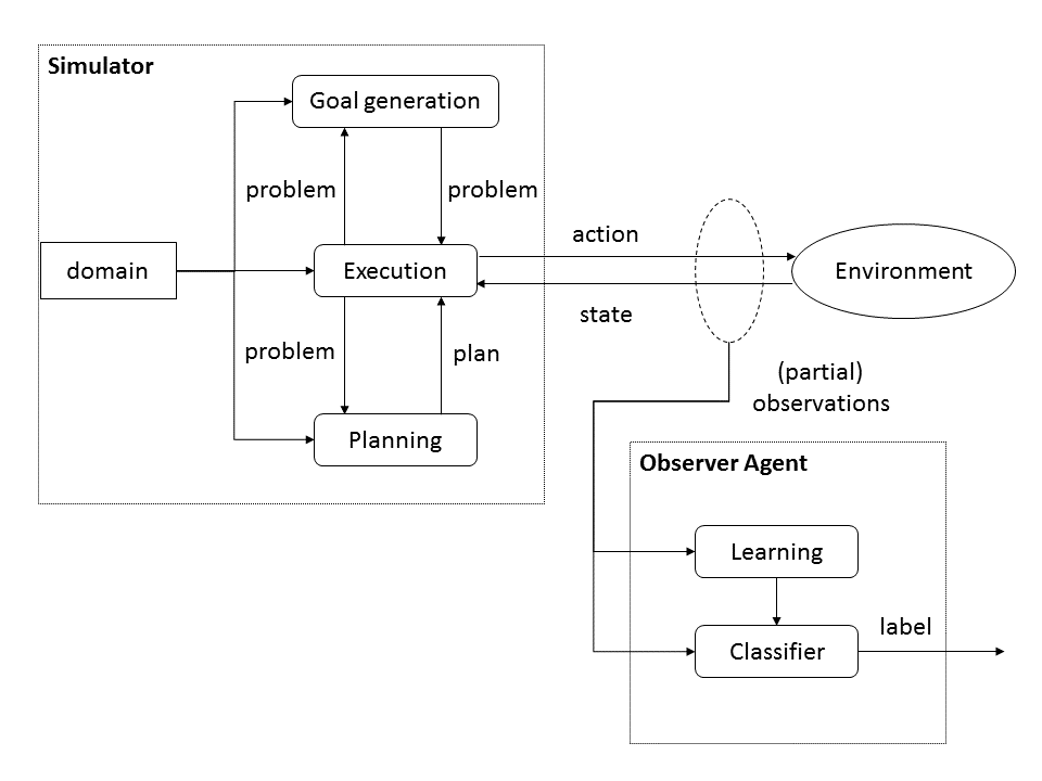
Figure 1: High level view of the simulator.

5.1 Domain Model

We model the domain with PDDL (Planning Domain Description Language), that allows for a compact representation of planning tasks [Ghallab et al., 1998]. We define a common domain model for both behaviors (standard and criminal). It includes: a hierarchy of types (e.g. account, company, or customer); a set of predicates and functions (Tables 1 and 2); and a set of actions (Table 3).

Different planning problems can be defined within a domain. They consist of: (1) a set of objects, such as customers, accounts, companies, and transactions; (2) an initial state that, in our case, is the same for both kinds of behavior except that it contains information on a customer being a criminal for bad behaviors; and (3) a set of goals, that is initially empty as they will be dynamically generated by the goals generation component.

We have modeled some examples of known behavior for money laundering [Irwin et al., 2012]. Standard money laundering is composed of placement, layering and integration. Placement consists of introducing the money with illicit origin into the financial system. We have implemented two different ways of performing placement: depositing money directly into bank accounts, or moving digital money to standard accounts. Layering consists on moving placed money into other accounts to make tracing the origin/destination of money difficult. Integration consists on using that money for standard operations. We have implemented three integration strategies: withdrawal, paying bills, or international money transfer. All these decisions are made randomly according to some probability distributions.

5.2 Execution

At each simulation step, the execution component calls the planning component if there is a reason for (re)planning. Reasons for replanning are: the new state is not the expected one; or goal generation has returned new goals. If there is a plan in execution, it simulates its execution in the environment. Our simulator includes the possibility of defining deterministic and non-deterministic execution of actions, and the appearance of exogenous events. At each step, the execution component calls goal generation for changes in the goals or partial descriptions of states, as explained below.

The interaction with the environment also generates a trace of observations that will be used for training and test of $F$ learning component. The trace contains a sequence of actions and states from the $F$ viewpoint. Hence, the execution applies a filter on both so that it includes only its observable elements in the trace. Each simulation finishes after a predefined number of simulation steps (horizon) that is a parameter, or after a plan was not found in two consecutive steps in a given time bound. We set the time bound with a low value (10 seconds), since this is enough in most cases.

5.3 Goal Generation

This component allows agents to generate realistic behavior whose goals evolve over time depending on the current state of the environment. It takes as input the current problem description (state, goals and instances) and returns a new problem description. The first obvious effect of this module is to change goals. In order to do so, we have defined two kinds of behavior by changing the goals of each type. In the case of persons doing money laundering, the simulator will dynamically generate goals corresponding to a pure bad behavior, such as committing a crime, or laundering money. But, the simulator will interleave these bad behavior goals with standard customer goals, so that the task of deciding whether some trace belongs to a bad behavior is not easy to detect. In the case of standard customer goals, the simulator would generate goals such as owning a house (or cheaper kinds of products or services), working for a company, creating a company, or making payments to an utility company. The generation of goals for both kinds of behavior is guided by some probability distributions that allow to easily change the types of traces generated.

This component can also change the state and instances. This is useful for generating new components of the state on-line. As an example, we do not want to include initially information about all transactions to be performed by $C$ during the complete simulation period. Instead, the Goal generation allows the simulator to define new objects or state components as needed. So, if it generates a goal of buying a product, it could generate a new customer – the seller–, her account, the product to be bought, and all the associated information in the state.

5.4 Planning

Planners take as input a domain and problem description in PDDL, and return a plan that solves the corresponding planning task. In principle, we could have used any PDDL complaint planner. However, we make extensive use of numeric variables (using PDDL functions). So, we are restricted to planners that can reason with numeric preconditions and effects. We are using cbp [Fuentetaja, 2011].

5.5 Experiments on Behavior Novelty

As a final experiment, we wanted to test the hypothesis that the learning system would be able to still correctly identify new unseen behavior, which would lead to a great advantage to AML investigation. In order to test the identification of novel behavior, we generated 10 training instances corresponding to a specific money laundering behavior (placement with cash deposits, usually called structuring) and also 10 training instances of standard customer behavior. Then, we generated 20 test instances randomly selecting good and bad behavior. However, now the bad behavior used placement with digital money. So, we were trying to test the ability of cabbot of correctly classifying unseen behavior. We used long traces of 350 steps. The result is that it correctly classified all test instances (100% accuracy). But it took it more observations than before to detect it; from an average of 2.75 when it saw both kinds of placement in the training instances, to 8.3 when it only saw cash deposits in the training instances and the test where using digital. In the case of the decision tree, it also had a 100% accuracy, but the average number of observations that it required to converge to the right decision was 50.95. When we reversed the training behavior (digital placement) and test behavior (cash deposits), we obtained equivalent results. These results are very encouraging from the point of real investigation, since the system is able to correctly classify unseen behavior (from a different probability distribution).

6 Conclusions

We have presented three main contributions. The first one consists of a new way of modeling the AML task as classification of relational-based behavior traces. The models of observed behaviors are richer that usual ones based on transactions only. They also allow to easily create different observation models and evaluate the impact of using them. The second contribution is cabbot, a relational learning technique that takes a set of training traces of other agents’s behavior and can classify later traces. We have used some known relational distances and have proposed a new one that explicitly considers the structure of the input examples (traces). The third contribution is a simulator that generates synthetic behaviors where agents can dynamically change their goals, and therefore their plans. The execution of those plans leaves a behavior trace that can be used by the learning system to classify new traces. The diversity of generated traces can be used to challenge the learning system, as well as it can be exploited by financial institutions to pro-actively study new kinds of behavior. Experimental results show that cabbot can successfully learn to classify new traces in the presence of different observability models. In future work, we would like to connect the learning component to real data, and automate the process of AML using the output of its decisions.

References

- [Chandola et al., 2010] Varun Chandola, Arindam Banerjee, and Vipin Kumar. Anomaly detection for discrete sequences: A survey. IEEE Transactions on Knowledge and Data Engineering, 24(5):823–839, 2010.
- [Chen and Mathe, 2011] Yu-To Chen and Johan Mathe. Fuzzy computing applications for anti-money laundering and distributed storage system load monitoring. In Proceedings of the World Conference on Soft Computing, 2011.
- [Chen et al., 2018] Z. Chen, L. Dinh, V. Khoa, A. Nazir, E.N. Teoh, E.K. Karupiah, and K.S. Lam. Machine learning techniques for anti-money laundering (AML) solutions in suspicious transaction detection: A review. Knowledge Information Systems, 57:245–285, 2018.
- [Dzeroski and Lavrac, 2010] Saso Dzeroski and Nada Lavrac. Relational Data Mining. Springer, 2010.
- [Emde and Wettschereck, 1996] W. Emde and D. Wettschereck. Relational instance based learning. In Lorenza Saitta, editor, Machine Learning - Proceedings 13th International Conference on Machine Learning, pages 122 – 130. Morgan Kaufmann Publishers, 1996.
- [Fronzetti Colladon and Remondi, 2017] Andrea Fronzetti Colladon and Elisa Remondi. Using social network analysis to prevent money laundering. Expert Systems with Applications, 67:49–58, 2017.
- [Fuentetaja, 2011] Raquel Fuentetaja. The cbp planner. In Preprints of Workshop on International Planning Competition (IPC), ICAPS, 2011.
- [Ghallab et al., 1998] M. Ghallab, A. Howe, C. Knoblock, D. McDermott, A. Ram, M. Veloso, D. Weld, and D. Wilkins. PDDL - the planning domain definition language. Technical Report CVC TR-98-003/DCS TR-1165, Yale Center for Computational Vision and Control, 1998.
- [Gupta et al., 2013] Manish Gupta, Jing Gao, Charu C Aggarwal, and Jiawei Han. Outlier detection for temporal data: A survey. IEEE Transactions on Knowledge and Data Engineering, 26(9):2250–2267, 2013.
- [Irwin et al., 2012] Angela Irwin, Kim-Kwang Raymond Choo, and Lin Liu. Modelling of money laundering and terrorism financing typologies. Journal of Money Laundering Control, 15:316, 01 2012.
- [Isa et al., 2015] Yusarina Mat Isa, Zuraidah Mohd Sanusi, Mohd Nizal Haniff, and Paul A. Barnes. Money laundering risk: From the bankers’ and regulators perspectives. Procedia Economics and Finance, 28:7 – 13, 2015. 7th International Conference on Financial Criminology.
- [Jaccard, 1901] Paul Jaccard. Étude comparative de la distribution florale dans une portion des alpes et des jura. Bulletin de la Société Vaudoise des Sciences Naturelles, 37:547–579, 1901.
- [Kingdon, 2004] J. Kingdon. Ai fights money laundering. Intelligent Systems, IEEE, 19:87 – 89, 06 2004.
- [Larik and Haider, 2011] Asma S. Larik and Sajjad Haider. Clustering based anomalous transaction reporting. Procedia Computer Science, 3:606 – 610, 2011. World Conference on Information Technology.
- [Lin-Tao et al., 2008] Lv Lin-Tao, Ji Na, and Zhang Jiu-Long. A rbf neural network model for anti-money laundering. In Proceedings of the International Conference on Wavelet Analysis and Pattern Recognition, 2008.
- [Lopez-Rojas and Axelson, 2012] E. A. Lopez-Rojas and S. Axelson. Money laundering detection using synthetic data. In The 27th workshop of Swedish Artificial Intelligence Society (SAIS), pages 33–40, 2012.
- [Luo, 2014] X Luo. Suspicious transaction detection for anti-money laundering. International Journal of Security and Its Applications, 8(2):157–166, 2014.
- [Ontañón, 2020] Santiago Ontañón. An overview of distance and similarity functions for structured data. Artificial Intelligence Review, pages 1–43, 2020.
- [Rajput et al., 2014] Quratulain Rajput, Nida Khan, Asma Larik, and Sajjad Haider. Ontology based expert-system for suspicious transactions detection. Computer and Information Science, 7, 10 2014.
- [Raza and Haider, 2011] Saleha Raza and Sajjad Haider. Suspicious activity reporting using dynamic bayesian networks. Procedia Computer Science, 3:987 – 991, 2011. World Conference on Information Technology.
- [Schlichtkrull et al., 2018] Michael Schlichtkrull, Thomas N Kipf, Peter Bloem, Rianne Van Den Berg, Ivan Titov, and Max Welling. Modeling relational data with graph convolutional networks. In European Semantic Web Conference, pages 593–607. Springer, 2018.
- [Senator et al., 1995] Ted E. Senator, Henry G. Goldberg, Jerry Wooton, Matthew A. Cottini, A.F. Umar Khan, Christina D. Klinger, Winston M. Llamas, Michael P. Marrone, and Raphael W.H. Wong. The FinCEN artificial intelligence system: Identifying potential money laundering from reports of large cash transactions. In Proceedings of IAAI, 1995.
- [Takáts, 2011] Előd Takáts. A theory of “crying wolf”: The economics of money laundering enforcement. The Journal of Law, Economics, & Organization, 27(1):32–78, 2011.
- [van der Aalst, 2016] Wil van der Aalst. Process Mining: Data Science in Action. Springer, 2016.
- [Wang and Yang, 2008] Su-Nan Wang and Jian-Gang Yang. A money laundering risk evaluation method based on decision tree. In Proceedings of the International Conference on Machine Learning and Cybernetics, 2008.
- [Weber et al., 2018] Mark Weber, Jie Chen, Toyotaro Suzumura, Aldo Pareja, Tengfei Ma, Hiroki Kanezashi, Tim Kaler, Charles E Leiserson, and Tao B Schardl. Scalable graph learning for anti-money laundering: A first look. arXiv preprint arXiv:1812.00076, 2018.