Doubly Robust Off-Policy Learning on Low-Dimensional Manifolds by Deep Neural Networks

Abstract

Causal inference explores the causation between actions and the consequent rewards on a covariate set. Recently deep learning has achieved a remarkable performance in causal inference, but existing statistical theories cannot well explain such an empirical success, especially when the covariates are high-dimensional. Most theoretical results in causal inference are asymptotic, suffer from the curse of dimensionality, and only work for the finite-action scenario. To bridge such a gap between theory and practice, this paper studies doubly robust off-policy learning by deep neural networks. When the covariates lie on a low-dimensional manifold, we prove nonasymptotic regret bounds, which converge at a fast rate depending on the intrinsic dimension of the manifold. Our results cover both the finite- and continuous-action scenarios. Our theory shows that deep neural networks are adaptive to the low-dimensional geometric structures of the covariates, and partially explains the success of deep learning for causal inference.

1 Introduction

Causal inference studies the causal connection between actions and rewards, which has wide applications in healthcare (Kim et al., 2011; Lunceford and Davidian, 2004), digital advertising (Farias and Li, 2019), product recommendation (Sharma et al., 2015), and policy formulation (Heckman and Vytlacil, 2007). For example in healthcare, each patient can be characterized by a set of covariates (also called features), and the actions are a set of treatments. Each patient has the corresponding reactions, or rewards, to different treatments. Causal inference enables one to personalize the treatment to each patient to maximize the total rewards. Such a personalized decision-making rule is referred to as a policy, which is a map from the covariate set to the action set. In off-policy learning, a batch of observational data is given, which typically consists of a covariate (also called a feature), the action taken (e.g. medical treatments and recommendations), and the observed reward. In this paper, we are interested in learning an optimal policy that targets personalized treatments or services to different individuals based on the logged data. This is also known as the optimal treatment assignment in literature (Rubin, 1974; Heckman, 1977).

Conventional causal inference methods often rely on parametric models (Lunceford and Davidian, 2004; Cao et al., 2009; Robins et al., 1994; Kitagawa and Tetenov, 2018), which can introduce a large bias when the real model is not in the assumed parametric form. Many nonparametric methods are proposed (Hill, 2011; Kitagawa and Tetenov, 2018; Zhao et al., 2015; Kennedy et al., 2017; Richardson et al., 2014; Chan et al., 2016; Frölich et al., 2017; Benkeser et al., 2020; Kennedy, 2020; Lee et al., 2020; Crump et al., 2008; Benkeser et al., 2017), while the statistical theories often suffer from the curse of dimensionality. Recently neural networks became a popular modeling tool for causal inference. Many results have shown that neural networks outperform conventional nonparametric approaches, especially when the learning task involves high-dimensional complex data. For example, Lopez-Paz et al. (2017) proposed to discover causal and anticausal features in images from ImageNet using a $20$-layer residual network. Pham and Shen (2017) used recurrent neural networks to study the causality between group forming loans and the funding time on an online non-profit financial platform. Other examples can be found in diverse areas, including climate analysis, medical diagnosis, cognitive science, and online recommendations (Chalupka et al., 2014; van Amsterdam et al., 2019; Johansson et al., 2016; Hartford et al., 2017; Zhang et al., 2019; Lim, 2018).

Despite the great progress of causal inference, there is still a huge gap between theory and practice. In casual inference, many existing theories on nonparametric or neural networks approaches are asymptotic, and suffer from the curse of dimensionality. Specifically, to achieve an $\epsilon$ accuracy, the sample complexity needs to grow in the order of $\epsilon^{-D}$, where $D$ is the covariate dimension. Such theories can not explain the empirical success when $D$ is large. For example, in Lopez-Paz et al. (2017), the RGB images in ImageNet are of resolution $3\times 224\times 224$. To obtain a $0.1$ error, the sample complexity needs to scale like $10^{-3\times 224\times 224}$, which well exceeds the training size of $99,309$. Besides, the curse of dimensionality is inevitable unless additional data structures are considered. Gao and Han (2020) proved that, for binary policy learning problems, the sample complexity obtained by the optimal algorithm still grows exponentially in the covariate dimension $D$ in the order of $\epsilon^{-D}$.

To bridge this gap, we take the low-dimensional geometric structures of the covariates into consideration. This is motivated by the fact that real-world data often exhibit low-dimensional structures, due to rich local regularities, global symmetries, or repetitive patterns (Tenenbaum et al., 2000; Roweis and Saul, 2000; Peyré, 2009). For example, many images describe the same object with different transformations, like translation, rotation, projection and skeletonization. These transformations are often represented by a small number of parameters, including the translation position, the rotation, and the projection angle, etc. Similar low-dimensional structures exist in medical data (Choi et al., 2016; Mahoney and Drineas, 2009) and financial data (Baptista et al., 2000). To incorporate such low-dimensional structures of data, we assume that the input covariates are concentrated on a $d$-dimensional Riemannian manifold embedded in $\mathbb{R}^{D}$ with $d\ll D$.

In many off-policy learning methods, policy evaluation plays an important role by evaluating the expected reward of a given policy. Most of the existing works dedicate to policy evaluation with finite actions. Only few works addressed the continuous action scenario (Kallus and Zhou, 2018b; Demirer et al., 2019; Kallus and Santacatterina, 2019). Among the policy evaluation methods with finite actions, the doubly robust method (Cassel et al., 1976; Robins et al., 1994; Dudík et al., 2011) has the advantage of being consistent, if either the reward function or the propensity score (the probability of choosing a certain action given the covariate) is correctly specified. The statistical theory for policy evaluation has been intensively studied in the past with many asymptotic results (Swaminathan and Joachims, 2015; Zhou et al., 2018; Zhao et al., 2012; Kallus and Zhou, 2018a; Kitagawa and Tetenov, 2018).

This paper establishes statistical guarantees of policy learning in causal inference using neural networks. We consider the doubly robust method (see Section 3 for details), and use deep ReLU neural networks to parameterize the policy class, the propensity score, and the conditional expected reward. We prove nonasymptotic regret bounds which converge at a fast rate depending on the intrinsic dimension $d$, instead of the covariate dimension $D$. Furthermore, our theory applies to both the finite-action and continuous-action scenarios.

This paper has three main contributions: 1) By taking the low-dimensional geometric structures of the covariates into consideration, we prove a fast convergence rate of the learned policy, depending on the intrinsic dimension of the covariates. 2) Our statistical theory is nonasymptotic for policy learning, while most existing works established asymptotic theories for policy evaluation using the doubly robust method. While policy evaluation gives rise to the performance of any specific policy, policy learning furhter returns an optimal policy. 3) To our best knowledge, we prove the first regret bound of policy learning in a continuous action space.

Related work

In off-policy learning, one line of research learns the optimal policy by evaluating the expected reward of candidate policies and then finding the policy with the largest expected reward. The procedure of evaluating a target policy from the given data is called off-policy evaluation, which has been intensively studied in literature. The simplest way to evaluate a policy is the direct method which estimates the empirical reward of the target policy from collected data (Beygelzimer and Langford, 2009). The direct method is unbiased if one specifies the reward model correctly. However, model specification is a difficult task in practice. Another method is the inverse propensity weighting (Horvitz and Thompson, 1952; Robins et al., 1994), which uses the importance weighting to correct the mismatch between the propensity scores of the target policy and the data collection policy. This method is unbiased if the data collection policy can be exactly estimated, yet it has a large variance especially when some actions are rarely observed. A more robust method is the doubly robust method (Cassel et al., 1976; Cao et al., 2009; Dudík et al., 2011), which integrates the direct method and the inverse propensity weighting. This method is unbiased if the reward model is correctly specified or the data collection policy is known.

The aforementioned methods have been used in Kitagawa and Tetenov (2018); Zhao et al. (2015); Athey and Wager (2017); Zhou et al. (2018) for off-policy learning. Kitagawa and Tetenov (2018) used the inverse propensity weighting, and Athey and Wager (2017) and Zhao et al. (2015) used the doubly robust method to learn the optimal policy with binary actions. In Zhou et al. (2018), an algorithm based on decision trees was proposed to learn the optimal policy with multiple actions using the doubly robust method. Kallus (2018) proposed a balanced method which minimizes the worst-case conditional mean squared error to evaluate and learn the optimal policy with multiple actions.

Another line of research learns the optimal policy without evaluating policies. In Zhang et al. (2012); Zhao et al. (2012), the authors transformed the policy learning task with binary actions into a classification problem. Other works on off-policy learning include Kallus (2020); Ward et al. (2019), and Bennett and Kallus (2020).

Most of the aforementioned works provide asymptotic regret bounds with finite actions, which are valid when the number of samples goes to infinity. A nonasymptotic bound was derived in Kitagawa and Tetenov (2018), but this work requires that the propensity score is known and the algorithm only works for policy learning with binary actions. Meanwhile, off-policy learning with continuous actions has not been addressed until recently (Kallus and Zhou, 2018b; Demirer et al., 2019; Kallus and Santacatterina, 2019). Demirer et al. (2019) developed a semi-parametric off-policy learning algorithm, which requires the reward function in a specific class. Kallus and Zhou (2018b) applied a kernel method to extend the inverse propensity weighting and the doubly robust method to the continuous-action setting. These works on continuous actions did not provide a nonasymptotic regret bound with an explicit dependency on the number of samples.

The rest of the paper is organized as follows: Section 2 introduces manifold and neural networks; Section 3 presents the doubly robust estimation framework; Section 4 states our regret bounds of the learned policy; Section 5 gives a proof sketch of our theory; Section 6 discusses several related topics.

Notations: We use bold lowercase letters to denote vectors, i.e., $\bm{x}\in\mathbb{R}^{D}$. We use $x_{i}$ to denote the $i$-th entry of $\bm{x}$, and define $|\bm{x}|=\sum_{i=1}^{D}|x_{i}|$ and $\left\lVert\bm{x}\right\rVert_{2}^{2}=\sum_{i=1}^{D}x_{i}^{2}$. For a function $f:\mathbb{R}^{D}\rightarrow\mathbb{R}$ and a multi-index $\bm{s}=[s_{1},\dots,s_{D}]^{\top}$, $\partial^{\bm{s}}f$ denotes $\partial^{|\bm{s}|}f/\partial x_{1}^{s_{1}}\cdots\partial x_{D}^{s_{D}}$. Let $\Omega$ be the support of a probability distribution $\mathbb{P}$. The $L_{2}$ norm of $f$ with respect to $\mathbb{P}$ is denoted as $\|f\|^{2}_{L_{2}}=\int_{\Omega}f^{2}(\bm{x})d\mathbb{P}(\bm{x})$. We use $\circ$ to denote function composition. For a set $\mathcal{A}$, $|\mathcal{A}|$ denotes its cardinality. For a scalar $a>0$, $\lfloor a\rfloor$ denotes the largest integer which is no larger than $a$, $\lceil a\rceil$ denotes the smallest integer which is no smaller than $a$. For $a,b\in\mathbb{R}$, we denote $a\vee b=\max\{a,b\}$ and $a\wedge b=\min\{a,b\}$. We refer to a one-hot vector as a canonical basis, i.e. $\bm{v}_{j}=[0,\dots,0,1,0,\dots,0]^{\top}\in\mathbb{R}^{d}$ with $j$-th element being $1$. We use $\coloneqq$ to define important quantities.

2 Preliminaries on Manifold and Neural Networks

We briefly review smooth manifolds (see Lee (2003) and Tu (2010) for more details), Hölder space on a smooth manifold, and define the neural network class considered throughout this paper.

2.1 Low-Dimensional Manifold

Let $\mathcal{M}$ be a $d$-dimensional Riemannian manifold isometrically embedded in $\mathbb{R}^{D}$. A chart for $\mathcal{M}$ is a pair $(U,\phi)$ such that $U\subset\mathcal{M}$ is open and $\phi:U\rightarrow\mathbb{R}^{d}$ is a homeomorphism, i.e., $\phi$ is a bijection, its inverse and itself are continuous. Two charts $(U,\phi)$ and $(V,\psi)$ are called $C^{k}$ compatible if and only if the transition functions

$$\phi\circ\psi^{-1}:\psi(U\cap V)\rightarrow\phi(U\cap V)\quad\mbox{ and }\quad\psi\circ\phi^{-1}:\phi(U\cap V)\rightarrow\psi(U\cap V)$$

are both $C^{k}$ functions. A $C^{k}$ atlas of $\mathcal{M}$ is a collection of $C^{k}$ compatible charts $\{(U_{i},\phi_{i})\}$ such that $\bigcup_{i}U_{i}=\mathcal{M}$. An atlas of $\mathcal{M}$ contains an open cover of $\mathcal{M}$ and the mappings from each open cover to $\mathbb{R}^{d}$.

Definition 1 (Smooth manifold).

A manifold $\mathcal{M}$ is smooth if it has a $C^{\infty}$ atlas.

Through the concept of atlas, we are able to define $C^{s}$ functions and Hölder space on a smooth manifold.

Definition 2 ($C^{s}$ functions on $\mathcal{M}$).

Let $\mathcal{M}$ be a smooth manifold and fix a $C^{\infty}$ atlas of it. For a function $f:\mathcal{M}\rightarrow\mathbb{R}$, we say $f$ is a $C^{s}$ function on $\mathcal{M}$ if for any $(U,\phi)$ in the atlas, $f\circ\phi^{-1}$ is a $C^{s}$ function in $\mathbb{R}^{d}$.

Definition 3 (Hölder space on $\mathcal{M}$).

Let $\mathcal{M}$ be a compact manifold. A function $f:\mathcal{M}\mapsto\mathbb{R}$ belongs to the Hölder space $\mathcal{H}^{\alpha}(\mathcal{M})$ with a Hölder index $\alpha>0$, if for any chart $(U,\phi)$, we have

$$\|f\|_{\mathcal{H}^{\alpha}(U)} =\max_{|\bm{s}|<\lceil\alpha-1\rceil}\sup\limits_{\bm{x}\in\phi(U)}|\partial^{\bm{s}}f\circ\phi^{-1}(\bm{x})|+\max\limits_{|\bm{s}|=\lceil\alpha-1\rceil}\sup\limits_{\bm{x}\neq\bm{y}\in\phi(U)}\frac{|\partial^{\bm{s}}f\circ\phi^{-1}(\bm{x})-\partial^{\bm{s}}f\circ\phi^{-1}(\bm{y})|}{\|\bm{x}-\bm{y}\|_{2}^{\alpha-\lceil\alpha-1\rceil}}<\infty.$$

For a fixed atlas $\{(U_{i},\phi_{i})\}$, the Hölder norm of $f$ is defined as $\left\lVert f\right\rVert_{\mathcal{H}^{\alpha}(\mathcal{M})}=\sup_{i}\|f\|_{\mathcal{H}^{\alpha}(U_{i})}$. We occasionally omit $\mathcal{M}$ in the Hölder norm when it is clear from the context.

We introduce the reach (Federer, 1959; Niyogi et al., 2008) of a manifold to characterize the local curvature of $\mathcal{M}$.

Definition 4 (Reach).

The medial axis of $\mathcal{M}$ is defined as

$${\mathcal{T}}(\mathcal{M})=\{\bm{x}\in\mathbb{R}^{D}~{}|~{}\exists~{}\bm{x}_{1}\neq\bm{x}_{2}\in\mathcal{M},\textrm{~{}such that~{}}\|\bm{x}-\bm{x}_{1}\|_{2}=\|\bm{x}-\bm{x}_{2}\|_{2}=\inf_{\bm{y}\in\mathcal{M}}\left\lVert\bm{x}-\bm{y}\right\rVert_{2}\}.$$

The reach $\tau$ of $\mathcal{M}$ is the minimum distance between $\mathcal{M}$ and ${\mathcal{T}}(\mathcal{M})$, i.e.

$$\tau=\inf_{\bm{x}\in{\mathcal{T}}(\mathcal{M}),\bm{y}\in\mathcal{M}}\|\bm{x}-\bm{y}\|_{2}.$$

Roughly speaking, reach measures how fast a manifold “bends” — a manifold with a large reach “bends” relatively slowly.

2.2 Neural Network

We focus on feedforward neural networks with the ReLU activation function: $\mathrm{ReLU}(x)=\max\{0,x\}$. When the argument is a vector or matrix, ReLU is applied entrywise. Given an input $\bm{x}$, an $L$-layer network computes an output as

$$f(\bm{x})=W_{L}\cdot\mathrm{ReLU}\left(W_{L-1}\cdots\mathrm{ReLU}(W_{1}\bm{x}+\bm{b}_{1})+\cdots+\bm{b}_{L-1}\right)+\bm{b}_{L},$$ (2.1)

where the $W_{i}$’s are weight matrices and $\bm{b}_{i}$’s are intercepts. We define a class of neural networks as

$$\mathcal{F}(L,p,K,\kappa,R)= \{f~{}|~{}f\mbox{ has the form of (\ref{eq.ReLU}) with }L\mbox{ layers and width bounded by }p,\|f\|_{\infty}\leq R,$$

$$\qquad\sum_{i=1}^{L}\|W_{i}\|_{0}+\|\bm{b}_{i}\|_{0}\leq K,\|W_{i}\|_{\infty,\infty}\leq\kappa,\|\bm{b}_{i}\|_{\infty}\leq\kappa\mbox{ for }i=1,...,L\},$$

where $\left\lVert H\right\rVert_{\infty,\infty}=\max_{i,j}|H_{ij}|$ for a matrix $H$ and $\|\cdot\|_{0}$ denotes the number of non-zero elements of its argument.

3 Off-Policy Learning with Low-Dimensional Covariates

We introduce a two-stage policy learning scheme using neural networks. Suppose we receive $n$ i.i.d. triples $\{(\bm{x}_{i},\bm{a}_{i},y_{i})\}_{i=1}^{n}$, where $\bm{x}_{i}\in\mathcal{M}$ denotes a covariate independently sampled from an unknown distribution on $\mathcal{M}$, $\bm{a}_{i}\in\mathcal{A}$ denotes the action taken, and $y_{i}\in\mathbb{R}$ is the observed reward. To incorporate the low-dimensional geometric structures of the covariates, we assume $\mathcal{M}$ is a $d$-dimensional Riemannian manifold isometrically embedded in $\mathbb{R}^{D}$. The action space $\mathcal{A}$ can be either finite or continuous. For each covariate and action pair $(\bm{x},\bm{a})$, there is an associated random reward. We adopt the unconfoundedness assumption to simplify the model, which is commonly used in existing literature on causal inference (Wasserman, 2013; Zhou et al., 2018).

Assumption 1 (Unconfoundedness).

The reward is independent of $\bm{a}$ conditioned on $\bm{x}$.

To better interpret Assumption 1, we first consider a finite action space $\mathcal{A}=\{A_{1},\dots,A_{|\mathcal{A}|}\}$, where $A_{j}$ is a one-hot vector, i.e. $A_{j}=[0,\dots,0,1,0,\dots,0]^{\top}$ with $1$ appearing at the $j$-th position. Given the covariate $\bm{x}$, there is a reward $\{Y_{1}(\bm{x}),\dots,Y_{|\mathcal{A}|}(\bm{x})\}$ for each action, where the randomness of $Y_{j}(\bm{x})$ only depends on $\bm{x}$. The observed reward $y_{i}$ is a realization of $Y_{j}(\bm{x}_{i})$ with $\bm{a}_{i}=A_{j}$.

3.1 Policy Learning with Finite Actions

When the action space is finite, a policy $\pi:\mathcal{M}\rightarrow\Delta^{|\mathcal{A}|}$ maps a covariate on $\mathcal{M}$ to a vector on the $|\mathcal{A}|$-dimensional simplex

$$\Delta^{|\mathcal{A}|}=\left\{\bm{z}\in\mathbb{R}^{|\mathcal{A}|}:z_{i}\geq 0\text{ and }\sum_{i}z_{i}=1\right\}.$$

The $j$-th entry of $\pi(\bm{x})$ denotes the probability of choosing the action $A_{j}$ given $\bm{x}$. A policy in the interior of the simplex is called a randomized policy. If $\pi(\bm{x})$ is a one-hot vector, it is called a deterministic policy. The expected reward of deploying a policy $\pi$ is

$$Q(\pi) =\mathbb{E}[Y(\pi(\bm{x}))]=\mathbb{E}\left[\left\langle[Y_{1}(\bm{x}),\dots,Y_{|\mathcal{A}|}(\bm{x})]^{\top},\pi(\bm{x})\right\rangle\right].$$ (3.1)

We investigate the doubly robust approach (Cassel et al., 1976; Robins et al., 1994; Dudík et al., 2011) for policy learning, which consists of two stages. After receiving the training data, we split them into two groups

$${\mathcal{S}}_{1}=\{(\bm{x}_{i},\bm{a}_{i},y_{i})\}_{i=1}^{n_{1}}\quad\textrm{and}\quad{\mathcal{S}}_{2}=\{(\bm{x}_{i},\bm{a}_{i},y_{i})\}_{i=n_{1}+1}^{n}.$$ (3.2)

We denote $n_{2}=n-n_{1}$ and choose $n_{1},n_{2}$ to be proportional to $n$ such that $n_{1}/n$ is a constant. In the first stage, we solve nonparametric regression problems using ${\mathcal{S}}_{1}$ to estimate two important functions — the propensity score and the conditional expected reward. For any action $A_{j}$, the propensity score

$$e_{A_{j}}(\bm{x})\coloneqq\mathbb{P}(\bm{a}=A_{j}~{}|~{}\bm{x})$$

quantifies the probability of choosing $A_{j}$ given the covariate $\bm{x}$, and the expected reward of choosing $A_{j}$ is

$$\mu_{A_{j}}(\bm{x})\coloneqq\mathbb{E}[Y_{j}(\bm{x})~{}|~{}\bm{x}].$$

Substituting the definition above into (3.1), we can write

$$Q(\pi)=\mathbb{E}\left\langle[\mu_{A_{1}}(\bm{x}),...,\mu_{A_{|\mathcal{A}|}}(\bm{x})]^{\top},\pi(\bm{x})\right\rangle=\int_{\mathcal{M}}\left\langle[\mu_{A_{1}}(\bm{x}),...,\mu_{A_{|\mathcal{A}|}}(\bm{x})]^{\top},\pi(\bm{x})\right\rangle d\bm{x}.$$ (3.3)

In the second stage, we learn a policy using ${\mathcal{S}}_{2}$ based on our estimated $e_{A_{j}}$’s and $\mu_{A_{j}}$’s, which only requires that either the $e_{A_{j}}$’s or the $\mu_{A_{j}}$’s are accurately estimated.

$\bullet$ Stage 1: Estimating $\mu_{A_{j}}$ and $e_{A_{j}}$. For each action $A_{j}$, we use a neural network to estimate the reward function $\mu_{A_{j}}$ by minimizing the following empirical quadratic loss

$$\widehat{\mu}_{A_{j}}(\bm{x}) =\mathop{\mathrm{argmin}}_{f\in\mathcal{F}_{\rm NN}}~{}\frac{1}{n_{A_{j}}}\sum_{i=1}^{n_{1}}(y_{i}-f(\bm{x}_{i}))^{2}\mathds{1}\{\bm{a}_{i}=A_{j}\}\quad\textrm{with}\quad n_{A_{j}}=\sum_{i=1}^{n_{1}}\mathds{1}\{\bm{a}_{i}=A_{j}\},$$ (3.4)

where $\mathcal{F}_{\rm NN}:\mathcal{M}\rightarrow\mathbb{R}$ is a properly chosen network class defined in Lemma 1.

An estimator of the propensity score $e_{A_{j}}$ is obtained by minimizing the multinomial logistic loss. Let $\mathcal{G}_{\rm NN}:\mathcal{M}\mapsto\mathbb{R}^{|\mathcal{A}|-1}$ be a properly chosen network class defined in Lemma 1. We obtain $\widehat{e}_{A_{j}}(\bm{x})$ via

$$\widehat{g}(\bm{x}) =\mathop{\mathrm{argmin}}_{g\in\mathcal{G}_{\rm NN}}~{}\frac{1}{n_{1}}\sum_{i=1}^{n_{1}}-[g(\bm{x}_{i})^{\top},1]\bm{a}_{i}+\log\Big{(}1+\sum_{j=1}^{|\mathcal{A}|-1}\exp([g(\bm{x}_{i})]_{j})\Big{)},$$ (3.5)

$$\widehat{e}_{A_{j}}(\bm{x}) =\frac{\exp([\widehat{g}(\bm{x})]_{j})}{1+\sum_{j=1}^{|\mathcal{A}|-1}\exp([\widehat{g}(\bm{x})]_{j})}~{}\textrm{for~{}}j\leq|\mathcal{A}|-1,~{}\textrm{and}~{}~{}\widehat{e}_{A_{|\mathcal{A}|}}(\bm{x})=\frac{1}{1+\sum_{j=1}^{|\mathcal{A}|-1}\exp([\widehat{g}(\bm{x})]_{j})}.$$ (3.6)

Here $[g]_{j}$ denotes the $j$-th entry, and $[g^{\top},1]\in\mathbb{R}^{|\mathcal{A}|}$ is obtained by augmenting $g$ by $1$.

$\bullet$ Stage 2: Policy Learning. Given $\widehat{\mu}_{A_{j}}$ and $\widehat{e}_{A_{j}}$, we learn an optimal policy by maximizing a doubly robust empirical reward:

$$\widehat{Q}(\pi):=\frac{1}{n_{2}}\sum_{i=n_{1}+1}^{n}\pi(\bm{x}_{i})^{\top}\widehat{\Gamma}_{i}\quad\textrm{with}\quad\widehat{\Gamma}_{i}=\frac{y_{i}-\widehat{\mu}_{\bm{a}_{i}}(\bm{x}_{i})}{\widehat{e}_{\bm{a}_{i}}(\bm{x}_{i})}\cdot\bm{a}_{i}+[\widehat{\mu}_{A_{1}}(\bm{x}_{i}),\dots,\widehat{\mu}_{A_{|\mathcal{A}|}}(\bm{x}_{i})]^{\top}\in\mathbb{R}^{|\mathcal{A}|}.$$ (3.7)

A doubly robust optimal policy is learned by

$$\widehat{\pi}_{\rm DR}=\mathop{\mathrm{argmax}}_{\pi\in\Pi_{\rm NN}}~{}\widehat{Q}(\pi),$$ (3.8)

where $\Pi_{\rm NN}$ is a properly chosen network class (see Section 4 for the configurations of $\Pi_{\rm NN}$, e.g., (4.8) and (4.9)). The doubly robust reward $\widehat{Q}$ can tolerate a relatively large estimation error in either $\widehat{\mu}_{A_{j}}$ or $\widehat{e}_{A_{j}}$ (see the discussion after Theorem 1).

3.2 Policy Learning with Continuous Actions

Continuous actions, e.g. doses of drugs, often arise in applications, but there are limited studies on policy learning with continuous actions. In this paper, we consider the continuous action space $\mathcal{A}=[0,1]$ and use $a\in\mathcal{A}$ to denote an action. When the random action $a$ takes the value $A\in[0,1]$, we denote $Y(\bm{x},A)$ as its random reward. The propensity score and conditional expected reward are defined analogously to the finite action case:

$$e(\bm{x},A)\coloneqq\frac{d}{dA}\mathbb{P}(a\leq A,A\in\mathcal{A}~{}|~{}\bm{x})\quad\textrm{and}\quad\mu(\bm{x},A)\coloneqq\mathbb{E}[Y(\bm{x},A)~{}|~{}\bm{x}].$$

Note that $e(\bm{x},A)$ is a probability density function.

In this scenario, we can learn an optimal policy by replicating the two-stage scheme with a discretization technique on the continuous action space. Specifically, we uniformly partition the action space $\mathcal{A}$ into $V$ sub-intervals and denote $I_{j}=[(j-1)/V,j/V]$ for $j=1,\dots V$. Accordingly, we define the discretized propensity score and conditional expected reward for the sub-interval $I_{j}$ as

$$e_{I_{j}}(\bm{x})\coloneqq\mathbb{P}(a\in I_{j}~{}|~{}\bm{x})\quad\textrm{and}\quad\mu_{I_{j}}(\bm{x})\coloneqq\mathbb{E}[Y(\bm{x},a)\mathds{1}\{a\in I_{j}\}~{}|~{}\bm{x}]/e_{I_{j}}.$$ (3.9)

After the discretization on the action space, we identify all the actions $a$ belonging to a single sub-interval $I_{j}$ as the midpoint $A_{j}=(2j-1)/2V$ of $I_{j}$ and equips $A_{j}$ with the average expected reward $\mu_{I_{j}}$. After discretization, we resemble the setup in the finite-action scenario, and then apply the aforementioned two-stage doubly robust approach to learn a discretized policy concentrated on the $A_{j}$’s. In the first stage, we obtain $\widehat{\mu}_{I_{j}}$ and $\widehat{e}_{I_{j}}$ as estimators of $\mu_{I_{j}}$ and $e_{I_{j}}$, respectively. In the second stage, we use neural networks for policy learning by maximizing the discretized doubly robust empirical reward. Specifically, we define $I(a_{i})=I_{j}$ for $a_{i}\in I_{j}$ which maps the continuous action to the corresponding discretized sub-interval. For $a_{i}\in I_{j}$, we denote $\bm{a}_{i}\in\{0,1\}^{V}$ as the one-hot vector with the $j$-th element being $1$, which encodes the action $a_{i}$. The discretized doubly robust empirical reward is defined as

$$\widehat{Q}^{\rm(D)}(\pi)\coloneqq\frac{1}{n_{2}}\sum_{i=n_{1}+1}^{n}\left\langle\widehat{\Gamma}_{i}^{\rm(D)},\pi(\bm{x}_{i})\right\rangle~{}~{}\textrm{with}~{}~{}\widehat{\Gamma}_{i}^{\rm(D)}=\frac{y_{i}-\widehat{\mu}_{I(a_{i})}(\bm{x}_{i})}{\widehat{e}_{I(a_{i})}(\bm{x}_{i})}\cdot\bm{a}_{i}+[\widehat{\mu}_{I_{1}}(\bm{x}_{i}),\dots,\widehat{\mu}_{I_{V}}(\bm{x}_{i})]^{\top},$$ (3.10)

where the superscript $({\rm D})$ denotes the discretized quantities. We learn an optimal policy by solving the following maximization problem:

$$\widehat{\pi}_{\textrm{ C-DR}}=\mathop{\mathrm{argmax}}_{\pi\in\Pi_{{\rm NN}}}~{}\widehat{Q}^{\rm(D)}(\pi)$$ (3.11)

where $\Pi_{\rm NN}$ is a properly chosen neural network. See Section 4.2 for more details of the learning procedure, a proper choice of $V$, and the statistical guarantees of the learned policy.

4 Main Results

Our main results are nonasymptotic regret bounds (see Definition 5) on the policy learned by the two-stage scheme in Section 3, when the covariates are concentrated on a low-dimensional manifold.

The regret of a policy $\pi$ against a reference policy $\bar{\pi}$ is defined as the difference between their respective expected rewards. The formal definition is given as follows.

Definition 5.

Let $\bar{\pi}$ be a fixed reference policy. For any policy $\pi$, the regret of $\pi$ against $\bar{\pi}$ is

$$R(\bar{\pi},\pi)=Q(\bar{\pi})-Q(\pi).$$

Here $Q(\pi)$ is the expected reward either in the finite-action scenario defined in (3.1) or the continuous-action scenario which is defined later in (4.15). We consider two reference policies: 1) the optimal Hölder policy that maximizes the expected reward; 2) the unconstrained optimal policy that maximizes the expected reward. We establish high probability bounds on the regret of the learned policy for both discrete actions (Section 4.1) and continuous actions (Section 4.2).

4.1 Policy Learning with Finite Actions

Our theory is based on the following assumptions, including a manifold model for covariates, some standard assumptions on the smoothness of the propensity score and the reward.

Assumption 2.

$\mathcal{M}$ is a $d$-dimensional compact smooth manifold isometrically embedded in $\mathbb{R}^{D}$. There exists $B>0$ such that $\|\bm{x}\|_{\infty}\leq B$ whenever $\bm{x}\in\mathcal{M}$. The reach $\tau$ of $\mathcal{M}$ satisfies $\tau>0$.

Assumption A.3.

The propensity score and random reward satisfy:

• Overlap: $e_{A_{j}}(\bm{x})\geq\eta$ for $j=1,\dots,|\mathcal{A}|$, where $\eta>0$ is a constant;

• Bounded Reward: $Y_{j}(\bm{x})$ is bounded and has a bounded variance, i.e., $\sup_{\bm{x}\in\mathcal{M}}|Y_{j}(\bm{x})|\leq M_{1}$ and $\operatorname{{\rm Var}}[Y_{j}]\leq\sigma^{2}$ for any $j=1,\dots,|\mathcal{A}|$, where $M_{1}>0$ and $\sigma>0$ are constants.

Assumption A.3 is a standard assumption for statistical guarantees of all learning approaches using the inverse propensity score (Wasserman, 2013; Farrell et al., 2018; Zhou et al., 2018). Assumption A.3 implies that expected reward $\mu_{A_{j}}$ is bounded since $|\mu_{A_{j}}(\bm{x})|\leq\mathbb{E}[|Y_{j}(\bm{x})|~{}|~{}\bm{x}]\leq M_{1}$ for every $\bm{x}\in\mathcal{M}$.

Assumption A.4.

Given a Hölder index $\alpha\geq 1$, we assume $\mu_{A_{j}}(\bm{x})\in\mathcal{H}^{\alpha}(\mathcal{M})$ and $e_{A_{j}}(\bm{x})\in\mathcal{H}^{\alpha}(\mathcal{M})$ for $j=1,\dots,|\mathcal{A}|$. Moreover, for a fixed $C^{\infty}$ atlas of $\mathcal{M}$, there exists $M_{2}>0$ such that

$$\max_{j}\left\lVert\mu_{A_{j}}\right\rVert_{\mathcal{H}^{\alpha}}\leq M_{2}\quad\textrm{and}\quad\max_{j}\|\log e_{A_{j}}\|_{\mathcal{H}^{\alpha}}\leq M_{2}.$$

Thanks to Assumption A.3 (i), $e_{A_{j}}\in\mathcal{H}^{\alpha}$ implies $\log e_{A_{j}}\in\mathcal{H}^{\alpha}$ (see Lemma 9 in Appendix G). Now we are ready to derive the following estimation bounds for $\mu_{A_{j}}$ and $e_{A_{j}}$ using nonparametric regression techniques (Tsybakov, 2008). To simplify the notation, we denote

$$M=\max\{1,M_{1},2M_{2},-\log\eta\}.$$ (4.1)

4.1.1 Estimation Bounds of $\mu_{A_{j}}(\bm{x})$ and $e_{A_{j}}(\bm{x})$

By choosing networks

$$\mathcal{F}_{\rm NN}=\mathcal{F}(L_{1},p_{1},K_{1},\kappa_{1},R_{1})\quad\textrm{and}\quad\mathcal{G}_{\rm NN}=\mathcal{F}(L_{2},p_{2},K_{2},\kappa_{2},R_{2})$$ (4.2)

to estimate $\mu_{A_{j}}$ and $e_{A_{j}}$ in (3.4) and (3.6), respectively, we prove the following estimation error bounds for the estimators $\widehat{\mu}_{A_{j}}$ and $\widehat{e}_{A_{j}}$ (Lemma 1 is proved in Appendix A). We use $O(\cdot)$ to hide absolute constants and polynomial factors of $\alpha$, Hölder norm, $\log D$, $d$, $\tau$, $|\mathcal{A}|$, and the surface area of $\mathcal{M}$.

Lemma 1.

Suppose Assumptions 1 – 2 and A.3 – A.4 hold. We choose

$$L_{1}=O(\log\eta n_{1}),\quad p_{1}=O\big{(}(\eta n_{1})^{\frac{d}{2\alpha+d}}\big{)},\quad K_{1}=O\big{(}(\eta n_{1})^{\frac{d}{2\alpha+d}}\log\eta n_{1}\big{)},$$ (4.3)

$$\hskip 72.26999pt\kappa_{1}=\max\{B,M,\sqrt{d},\tau^{2}\},\quad R_{1}=M$$

for $\mathcal{F}_{\rm NN}$ and

$$L_{2}=O(\log n_{1}),\ p_{2}=O\big{(}n_{1}^{\frac{d}{2\alpha+d}}\big{)},\ K_{2}=O\big{(}n_{1}^{\frac{d}{2\alpha+d}}\log n_{1}\big{)},\ \kappa_{2}=\max\{B,M,\sqrt{d},\tau^{2}\},\ R_{2}=M,$$ (4.4)

for $\mathcal{G}_{\rm NN}$ in (4.2). Then for any $j=1,\dots,|\mathcal{A}|$, we have

$$\mathbb{E}_{{\mathcal{S}}_{1}}\left[\left\lVert\widehat{\mu}_{A_{j}}-\mu_{A_{j}}\right\rVert_{L^{2}}^{2}\right] \leq C_{1}(M^{2}+\sigma^{2})(\eta n_{1})^{-\frac{2\alpha}{2\alpha+d}}\log^{3}(\eta n_{1}),$$ (4.5)

$$\mathbb{E}_{{\mathcal{S}}_{1}}\left[\left\lVert\widehat{e}_{A_{j}}-e_{A_{j}}\right\rVert_{L^{2}}^{2}\right] \leq C_{2}M^{2}|\mathcal{A}|^{\frac{4\alpha}{2\alpha+d}}n_{1}^{-\frac{2\alpha}{2\alpha+d}}\log^{3}n_{1},$$ (4.6)

where $C_{1},C_{2}$ depend on $\log D$, B, $\tau$ and the surface area of $\mathcal{M}$.

In (4.5) and (4.6), the expectation is taken with respect to ${\mathcal{S}}_{1}$ defined in (3.2). Lemma 1 provides performance guarantees of neural networks to solve regression problems (3.4) and (3.6) in order to estimate $\mu_{A_{j}}$ and $e_{A_{j}}$. When the covariates $\bm{x}$ are on a manifold, we prove that the estimation errors converge at a fast rate in which the exponent only depends on the intrinsic dimension $d$ instead of the ambient dimension $D$.

4.1.2 Regret Bound of Learned Policy versus Constrained Oracle Policy

Our first main result is a regret bound of $\widehat{\pi}_{\rm DR}$ obtained in (3.8) against the oracle policy in a Hölder policy class:

$$\pi_{\beta}^{*}=\mathop{\mathrm{argmax}}_{\pi\in\Pi_{\mathcal{H}^{\beta}}}\mathbb{E}[Q(\pi(\bm{x}))],$$

where the Hölder policy class $\Pi_{\mathcal{H}^{\beta}}$ is defined as

$$\Pi_{\mathcal{H}^{\beta}}\coloneqq\left\{\textrm{Softmax}[\nu_{1}(\bm{x}),\dots,\nu_{|\mathcal{A}|}(\bm{x})]^{\top}:\nu_{j}\in\mathcal{H}^{\beta}(\mathcal{M})\textrm{~{} and $\left\lVert\nu_{j}\right\rVert_{\mathcal{H}^{\beta}}\leq M$ for~{}}j=1,\dots,|\mathcal{A}|\right\}.$$ (4.7)

Accordingly, we pick the neural network policy class as

$$\Pi_{\rm NN}^{|\mathcal{A}|}=\{\textrm{Softmax}(f)\text{ with }f:\mathcal{M}\rightarrow\mathbb{R}^{|\mathcal{A}|}\in\mathcal{F}(L_{\Pi},p_{\Pi},K_{\Pi},\kappa_{\Pi},R_{\Pi})\}.$$ (4.8)

Our first theorem shows that $\widehat{\pi}_{\rm DR}$ is a consistent estimator of the oracle Hölder policy $\pi^{*}_{\beta}$ as long as the network parameters $L_{\Pi},p_{\Pi},K_{\Pi},\kappa_{\Pi},R_{\Pi}$ are properly chosen.

Theorem 1.

Suppose Assumptions 1 – 2 and A.3 – A.4 hold. Under the setup in Lemma 1, if the network parameters of $\Pi_{\rm NN}^{|\mathcal{A}|}$ are chosen with

$$L_{\Pi}=O(\log n),\quad p_{\Pi}=O\big{(}|\mathcal{A}|n^{\frac{d}{2\beta+d}}\big{)},\quad K_{\Pi}=O\big{(}|\mathcal{A}|n^{\frac{d}{2\beta+d}}\log n\big{)},$$ (4.9)

$$\hskip 72.26999pt\kappa_{\Pi}=\max\{B,M,\sqrt{d},\tau^{2}\},\quad R_{\Pi}=M,$$

then with probability no less than $1-C_{1}|\mathcal{A}|n^{-\frac{\beta}{2\beta+d}}$ over the randomness of data ${\mathcal{S}}_{1}$ and ${\mathcal{S}}_{2}$, the following bound holds

$$R(\pi_{\beta}^{*},\widehat{\pi}_{\rm DR})\leq C|\mathcal{A}|^{2}n^{-\frac{\beta}{2\beta+d}}\log^{2}n$$

$$\qquad+\eta^{-1}|\mathcal{A}|\sqrt{\frac{1}{n_{2}}\sum_{i=n_{1}+1}^{n}\left(\widehat{\mu}_{A_{j}}(\bm{x}_{i})-\mu_{A_{j}}(\bm{x}_{i})\right)^{2}}\sqrt{\frac{1}{n_{2}}\sum_{i=n_{1}+1}^{n}\left(\widehat{e}_{A_{j}}(\bm{x}_{i})-e_{A_{j}}(\bm{x}_{i})\right)^{2}},$$ (4.10)

where $C_{1}>0$ is an absolute constant and $C$ depends on $\log D$, $d$, $B$, $M$, $\tau$, $\eta$, $\beta$, and the surface area of $\mathcal{M}$.

Theorem 1 is proved in Section 5.1. Theorem 1 corroborates the doubly robust property of $\widehat{\pi}_{\rm DR}$. The regret of $\widehat{\pi}_{\rm DR}$ is not sensitive to the individual estimation error of either $\widehat{\mu}_{A_{j}}$ or $\widehat{e}_{A_{j}}$, since the bound depends on the product of the estimation errors. Combining Theorem 1 and Lemma 1 yields the following corollary (see proof in Section 5.2).

Corollary 1.

Suppose Assumptions 1 – 2 and A.3 – A.4 hold. If the network structures are chosen as in Lemma 1 and Theorem 1, the following regret bound holds with probability no less than $1-C_{1}n^{-\frac{\alpha\wedge\beta}{2(\alpha\wedge\beta)+d}}\log^{3}n$

$$R(\pi_{\beta}^{*},\widehat{\pi}_{\rm DR})\leq C|\mathcal{A}|^{\frac{8\alpha+2d}{2\alpha+d}}n^{-\frac{\alpha\wedge\beta}{2(\alpha\wedge\beta)+d}}\log^{2}n$$ (4.11)

where $C_{1}$ is an absolute constant, and $C$ depends on $\log D$, $d$, $B$, $M$, $\sigma$, $\tau$, $\eta$, $\alpha$, $\beta$, and the surface area of $\mathcal{M}$.

In comparison with existing works, our theory has several advantages:

• By considering the low-dimensional geometric structures of the covariates, we obtain a fast rate depending on the intrinsic dimension $d$. Our theory partially justifies the success of off-policy learning by neural networks for high-dimensional data with low-dimensional structures.

• Our assumptions on the propensity score and expected reward are weak in the sense that the Hölder index $\alpha\geq 1$ can be arbitrary. In Farrell et al. (2018) and Zhou et al. (2018), the Hölder index $\alpha$ of the propensity score and expected reward needs to satisfy $2\alpha>D$. This condition is hard to satisfy when the covariates are high-dimensional, unless the $\mu_{A_{j}}$’s and $e_{A_{j}}$’s are super smooth with bounded high-order derivatives.

• Our theory is nonasymptotic, while most existing works focus on an asymptotic analysis (Zhou et al., 2018; Athey and Wager, 2017; Farrell et al., 2018).

4.1.3 Regret Bound of Learned Policy versus Unconstrained Optimal Policy

We have shown that neural networks can accurately learn an oracle Hölder policy in Corollary 1.

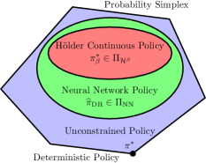
Figure 1: The unconstrained policy class is the whole probability simplex with vertices being deterministic polices. The inclusion relation of the neural network policy and the Hölder policy classes indicates that for any Hölder continuous policy, there is an approximation given by a neural network policy.

In this section, we enlarge the oracle policy class to capture all possible policies, including highly nonsmooth polices, e.g., deterministic policies. We show that neural networks can still achieve a small regret, due to their strong expressive power. The relationship between the Hölder policy class, neural network policy class, and unconstrained policy class is depicted in Figure 1.

The unconstrained optimal policy is defined as

$$\pi^{*}=\mathop{\mathrm{argmax}}_{\pi}~{}Q(\pi).$$

To establish the regret bound of $\widehat{\pi}_{\rm DR}$ in (3.8) against $\pi^{*}$, we need the following assumption on the $\mu_{A_{j}}$’s.

Assumption A.5 (Noise Condition).

Let $q\geq 1$ and denote $j^{*}(\bm{x})=\mathop{\mathrm{argmax}}_{j}\mu_{A_{j}}(\bm{x})$. There exists $c>0$, such that

$$\mathbb{P}\Big{[}\big{|}\mu_{A_{j^{*}(\bm{x})}}(\bm{x})-\max_{j\neq j^{*}(\bm{x})}\mu_{A_{j}}(\bm{x})\big{|}\leq Mt\Big{]}\leq ct^{q},\quad\text{ for any }t\in(0,1).$$

Assumption A.5 implies that, with high probability, there exists an optimal action whose expected reward is larger than those of others by a positive margin. This is an analogue of Tsybakov

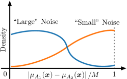
Figure 2: Noise condition in a binary-action scenario. “Large” noise corresponds to high densities when $\left|\mu_{A_{1}}(\bm{x})-\mu_{A_{2}}(\bm{x})\right|$ is small; “Small” noise corresponds to low densities near the origin.

low-noise condition (Tsybakov et al. (2004)) in multi-class classification problems, which appears similarly in Wang and Singh (2016). We illustrate the noise condition in a binary-action scenario in Figure 2.

We utilize a temperature parameter $H$ in the Softmax layer of the neural network to better learn the unconstrained optimal policy. Under the Hölder continuity in Assumption A.4, there exists a deterministic optimal policy $\pi^{*}$, i.e., $\pi^{*}(\bm{x})=A_{j^{*}(\bm{x})}$, which is a one-hot vector. In contrast, the output of the Softmax function is a randomized policy (i.e., a vector in the interior of the simplex), unless the output of the neural network is positive infinity. Accordingly, we adopt the Softmax function with a tunable temperature parameter $H$ to push the learned policy to a one-hot vector. This idea has given many empirical successes in reinforcement learning (Koulouriotis and Xanthopoulos, 2008; Kuleshov and Precup, 2014). Specifically, we set

$$\Pi_{{\rm NN}(H)}^{|\mathcal{A}|}=\{\textrm{Softmax}_{H}(f)~{}\textrm{with }f:\mathcal{M}\mapsto\mathbb{R}^{|\mathcal{A}|}\in\mathcal{F}(L_{\Pi},p_{\Pi},K_{\Pi},\kappa_{\Pi},R_{\Pi})\},$$ (4.12)

where $[\textrm{Softmax}_{H}(f)]_{i}=\frac{\exp(f_{i}/H)}{\sum_{j}\exp(f_{j}/H)}$. A small temperature $H$ will push the output of $\Pi^{|\mathcal{A}|}_{{\rm NN}(H)}$ towards a one-hot vector, which can better approximate the deterministic policy $\pi^{*}$.

Our main result is the following regret bound of $\widehat{\pi}_{\rm DR}$ (see proof in Section 5.3).

Theorem 2.

Suppose Assumptions 1 – 2 and A.3 – A.5 hold. Assume the network structures defined in Lemma 1 are used to estimate the $\mu_{A_{j}}$’s and the $e_{A_{j}}$’s. If the network parameters of $\Pi_{{\rm NN}(H)}^{|\mathcal{A}|}$ are chosen with

$$L_{\Pi}=O\left(\log n\right),\ p_{\Pi}=O\big{(}|\mathcal{A}|n^{\frac{d}{2\alpha+d}}\big{)},\ K_{\Pi}=O\big{(}|\mathcal{A}|n^{\frac{d}{2\alpha+d}}\log n\big{)},\ \kappa_{\Pi}=\max\{B,M,\sqrt{d},\tau^{2},1/H\},\ R_{\Pi}=M,$$

then the following bound holds with probability no less than $1-C_{1}n^{-\frac{\alpha}{2\alpha+d}}\log^{3}n$

$$R(\pi^{*},\widehat{\pi}_{\rm DR}) \leq\underbrace{C|\mathcal{A}|^{\frac{8\alpha+2d}{2\alpha+d}}n^{-\frac{\alpha}{2\alpha+d}}\log^{2}n\log^{1/2}\left(1/H\right)}_{{\mathcal{T}}_{1}}$$

$$\hskip 85.35826pt+\underbrace{\min_{t\in(0,1)}2cMt^{q}+M|\mathcal{A}|^{2}\exp\left[\left(-Mt+2n^{-\frac{\alpha}{2\alpha+d}}\right)/H\right]}_{{\mathcal{T}}_{2}},$$ (4.13)

where $C_{1}$ is an absolute constant, and $C$ depends on $\log D$, $d$, $B$, $M$, $\sigma$, $\tau$, $\eta$, $\alpha$, and the surface area of $\mathcal{M}$.

The regret $R(\pi^{*},\widehat{\pi}_{\rm DR})$ consists of two parts: a variance term ${\mathcal{T}}_{1}$ and a bias term ${\mathcal{T}}_{2}$. When the temperature $H$ is fixed, the variance ${\mathcal{T}}_{1}$ converges at the rate $n^{-\frac{\alpha}{2\alpha+d}}$, while the bias ${\mathcal{T}}_{2}$ does not vanish. This is because $\widehat{\pi}_{\rm DR}$ is a random policy as the output of a softmax function, while $\pi^{*}$ is deterministic as a one-hot vector under Assumption A.5. Furthermore, $\widehat{\pi}_{\rm DR}$ is asymptotically consistent with $\pi^{*}$ when $H\rightarrow 0$. If we choose $H=n^{-\frac{2\alpha}{2\alpha+d}}$ and $t=2n^{-\frac{\alpha}{2\alpha+d}}$, then ${\mathcal{T}}_{2}$ converges at the rate $n^{-\frac{q\alpha}{2\alpha+d}}$ and ${\mathcal{T}}_{1}$ converges at the rate $n^{-\frac{\alpha}{2\alpha+d}}$. We have the following corollary.

Corollary 2.

Suppose Assumptions 1 – 2 and A.3 – A.5 hold. In the setup of Theorem 2, setting $H=n^{-\frac{2\alpha}{2\alpha+d}}$ and $t=2n^{-\frac{\alpha}{2\alpha+d}}$ gives rise to

$$R(\pi^{*},\widehat{\pi}_{\rm DR})\leq C|\mathcal{A}|^{\frac{8\alpha+2d}{2\alpha+d}}n^{-\frac{(1\wedge q)\alpha}{2\alpha+d}}\log^{5/2}n$$ (4.14)

with probability no less than $1-C_{1}n^{-\frac{\alpha}{2\alpha+d}}\log^{3}n$, where $C_{1}$ is an absolute constant, and $C$ depends on $\log D$, $d$, $B$, $M$, $\sigma$, $\tau$, $\eta$, $\alpha$, and the surface area of $\mathcal{M}$.

4.2 Policy Learning with Continuous Actions

Our analysis can be extended to the continuous-action scenario. For simplicity, we let the action space be a unit interval, i.e., $\mathcal{A}=[0,1]$. In such a continuous-action scenario, a policy $\pi(\bm{x},\cdot)$, either randomized or deterministic, is a probability distribution on $[0,1]$ for each covariate $\bm{x}\in\mathcal{M}$. The expected reward of the policy $\pi$ is defined as

$$Q(\pi)=\int_{\mathcal{M}}\int_{0}^{1}\mu(\bm{x},A)\pi(\bm{x},A)dAd\mathbb{P}(\bm{x}),$$ (4.15)

where $\mathbb{P}$ is the marginal distribution of covariate $\bm{x}$.

As mentioned in Section 3.2, we tackle the continuous-action scenario using a discretization technique on the action space. This is motivated by practical applications where continuous objects are often quantized. The action space $\mathcal{A}$ is uniformly partitioned into $V$ sub-intervals $I_{j}=[(j-1)/V,j/V]$ for $j=1,\dots,V$, where $V$ is to be determined in Theorem 3. The discretized version of the propensity score and the expected reward on $I_{j}$ are defined in (3.9).

We also consider discretized policies on $\mathcal{A}$. In particular, we identify all the actions belonging to a single sub-interval $I_{j}$ as its midpoint $A_{j}=\frac{2j-1}{2V}$. A discretized policy is defined as

$$\pi^{\rm(D)}(\bm{x},A)=\sum_{j=1}^{V}p_{j}(\bm{x})\delta_{A_{j}}(A),$$ (4.16)

where $\delta_{A_{j}}$ is the Dirac delta function at $A_{j}$ and $p_{j}(\bm{x})$ denotes the probability of choosing action $A_{j}$, which satisifes $\sum_{j=1}^{V}p_{j}(\bm{x})=1$. In fact, $\pi^{\rm(D)}(\bm{x},\cdot)$ can be interpreted as a vector in the $V$-dimensional simplex, since it is only supported on $V$ discretized actions. For simplicity, we denote vector $\pi^{\rm(D)}(\bm{x})=[p_{1}(\bm{x}),\dots,p_{V}(\bm{x})]^{\top}$ with $p_{j}(\bm{x})$ representing the probability of choosing the action $A_{j}$, as an equivalent notation of $\pi^{\rm(D)}(\bm{x},\cdot)$.

For the discretized policy in (4.16), the discretized expected reward is defined as

$$Q^{\rm(D)}(\pi^{\rm(D)})=\int_{\mathcal{M}}\left\langle[\mu_{I_{1}}(\bm{x}),\dots,\mu_{I_{V}}(\bm{x})]^{\top},\pi^{\rm(D)}(\bm{x})\right\rangle d\mathbb{P}(\bm{x}).$$ (4.17)

We observe the analogy between (4.17) and (3.3) — the discrete conditional reward $\mu_{A_{j}}$ is replaced by the discretized conditional reward $\mu_{I_{j}}$, and the number of discrete actions $|\mathcal{A}|$ becomes the number of discretized actions $V$. On the other hand, the expected reward of a discretized policy is

$$Q(\pi^{\rm(D)}) =\int_{\mathcal{M}}\int_{0}^{1}\mu(\bm{x},A)\sum_{j=1}^{V}\pi_{j}(\bm{x})\delta_{A_{j}}(A)dAd\mathbb{P}(\bm{x})$$

$$=\int_{\mathcal{M}}\left\langle[\mu(\bm{x},A_{1}),\dots,\mu(\bm{x},A_{V})]^{\top},\pi^{\rm(D)}(\bm{x})\right\rangle d\mathbb{P}(\bm{x}).$$ (4.18)

The following lemma shows that if the $\mu(\bm{x},A)$ is Lipschitz in $A$ uniformly for any $\bm{x}\in\mathcal{M}$, $Q^{\rm(D)}(\pi^{\rm(D)})$ is close to $Q(\pi^{\rm(D)})$ when $V$ is large (see proof in Appendix B).

Lemma 2.

Assume there exists a constant $L_{\mu}>0$ such that

$$\sup_{\bm{x}\in\mathcal{M}}|\mu(\bm{x},A)-\mu(\bm{x},\widetilde{A})|\leq L_{\mu}|A-\widetilde{A}|\quad\textrm{for any}\quad A,\widetilde{A}\in[0,1].$$

Then for any discretized policy $\pi^{\rm(D)}$ given in (4.16), we have

$$|Q(\pi^{\rm(D)})-Q^{\rm(D)}(\pi^{\rm(D)})|\leq L_{\mu}/V.$$

We remark a key difference between (4.17) and (4.18). To evaluate (4.18), one needs to accurately estimate the $\mu(\bm{x},A_{j})$’s, which requires the action $A_{j}$ to be repeatedly observed. However, this is prohibitive in the continuous-action scenario, since an action $A_{j}$ is observed with probability $0$. In contrast, (4.17) relies on the average expected reward on a sub-interval, which can be estimated using standard nonparametric methods in the following Section 4.2.1. Moreover, thanks to Lemma 2, we can well approximate $Q(\pi^{\rm(D)})$ by $Q^{\rm(D)}(\pi^{\rm(D)})$ up to a small discretization error. This is crucial to establish the regret bound in Theorem 3.

4.2.1 Doubly Robust Policy Learning with Continuous Actions

After discretization, we can apply the doubly robust framework to learn an optimal discretized policy.

In the first stage, we estimate the $\mu_{I_{j}}$’s and $e_{I_{j}}$’s. In the sequel, we use the plain font $a_{i}$ to denote the observed action of the $i$-th sample. The bold font $\bm{a}_{i}\in\{0,1\}^{V}$ denotes the one-hot vector with the $j$-th element being $1$, if $a_{i}\in I_{j}$. Similar to (3.4) – (3.6) in the finite-action case, we obtain estimators of the $\mu_{I_{j}}$’s and $e_{I_{j}}$’s by minimizing the following empirical risks:

$$\widehat{\mu}_{I_{j}}(\bm{x}) =\mathop{\mathrm{argmin}}_{f\in\mathcal{F}_{\rm NN}}~{}\frac{1}{n_{I_{j}}}\sum_{i=1}^{n_{1}}(y_{i}-f(\bm{x}_{i}))^{2}\mathds{1}\{a_{i}\in I_{j}\}\quad\textrm{with}\quad n_{I_{j}}=\sum_{i=1}^{n_{1}}\mathds{1}\{a_{i}\in I_{j}\},$$ (4.19)

and

$$\widehat{g}(\bm{x})=\mathop{\mathrm{argmin}}_{g\in\mathcal{G}_{\rm NN}}~{}\frac{1}{n_{1}}\sum_{i=1}^{n_{1}}-\left\langle[g(\bm{x}_{i})^{\top},1]^{\top},\bm{a}_{i}\right\rangle+\log\Big{(}1+\sum_{j=1}^{V-1}\exp([g(\bm{x}_{i})]_{j})\Big{)},$$ (4.20)

$$\widehat{e}_{I_{j}}(\bm{x})=\frac{\exp([\widehat{g}(\bm{x})]_{j})}{1+\sum_{j=1}^{V-1}\exp([\widehat{g}(\bm{x})]_{j})}~{}\textrm{for~{}}j\leq V-1,~{}\textrm{and}~{}~{}\widehat{e}_{I_{V}}(\bm{x})=\frac{1}{1+\sum_{j=1}^{V-1}\exp([\widehat{g}(\bm{x})]_{j})},$$ (4.21)

where $\mathcal{F}_{\rm NN}:\mathcal{M}\rightarrow\mathbb{R}$ and $\mathcal{G}_{\rm NN}:\mathcal{M}\rightarrow\mathbb{R}^{V-1}$ are neural networks.

In the second stage, we learn an optimal discretized policy using the $\widehat{\mu}_{I_{j}}$’s and $\widehat{e}_{I_{j}}$’s. Recall that we define a mapping $I(a_{i}):=I_{j}$ for $a_{i}\in I_{j}$ to index which sub-interval $a_{i}$ belongs to. We use neural networks to learn a discretized policy by maximizing the doubly robust empirical reward in (3.10) and (3.11), i.e.,

$$\widehat{\pi}_{\text{ C-DR}}=\mathop{\mathrm{argmax}}_{\pi\in\Pi_{{\rm NN}(H)}^{V}}~{}\widehat{Q}^{\rm(D)}(\pi),$$ (4.22)

where $\Pi^{V}_{{\rm NN}(H)}$ represents the proper network class in (3.10), which is defined as (4.12). We emphasize that $\widehat{\pi}_{\textrm{C-DR}}$ is a discretized policy and the output $\widehat{\pi}_{\textrm{C-DR}}(\bm{x})$ is a $V$-dimensional vector in the simplex.

4.2.2 Regret Bound of Learned Discretized Policy

We begin with several assumptions, which are the continuous counterparts of Assumptions A.3 – A.5 in the finite-action scenario.

Assumption B.3.

The propensity score and random reward satisfy:

• Overlap: $e(\bm{x},A)\geq\eta$ for any $A\in\mathcal{A}$, where $\eta>0$ is a constant.

• Bounded Reward: $|Y(\bm{x},A)|\leq M_{1}$ for any $(\bm{x},A)\in\mathcal{M}\times[0,1]$, where $M_{1}>0$ is a constant.

Assumption B.4.

Given a Hölder index $\alpha\geq 1$, we have both the expected reward $\mu(\cdot,A)\in\mathcal{H}^{\alpha}(\mathcal{M})$ and the propensity score $e(\cdot,A)\in\mathcal{H}^{\alpha}(\mathcal{M})$ for any fixed action $A$. Moreover, the Hölder norms of $\mu(\cdot,A)$ and $e(\cdot,A)$ are uniformly bounded for any $A\in[0,1]$, i.e.,

$$\sup_{A\in[0,1]}\left\lVert\mu(\cdot,A)\right\rVert_{\mathcal{H}^{\alpha}}\leq M_{2},\quad\textrm{and}\quad\sup_{A\in[0,1]}\left\lVert e(\cdot,A)\right\rVert_{\mathcal{H}^{\alpha}}\leq M_{2}$$

for some constant $M_{2}>0$. Furthermore, there exists a constant $M_{3}>0$ such that

$$\sup_{\bm{x}\in\mathcal{M}}|\mu(\bm{x},A_{1})-\mu(\bm{x},A_{2})|\leq M_{3}|A_{1}-A_{2}|\quad\textrm{for any}~{}A_{1},A_{2}\in[0,1].$$

There also exists a constant $M_{4}>0$ such that

$$\left\lVert\log\left(\int_{I_{1}}e(\bm{x},A)dA/\int_{I_{2}}e(\bm{x},A)dA\right)\right\rVert_{\mathcal{H}^{\alpha}}\leq M_{4}\quad\textrm{for any intervals}~{}I_{1},I_{2}\subset[0,1]\textrm{ of the same length}.$$

Let $p_{I}(\bm{x})=\int_{I}e(\bm{x},A)dA$ denote the probability of choosing actions in $I$ given $\bm{x}$. In Assumption B.4, the condition $e(\cdot,A)\in\mathcal{H}^{\alpha}(\mathcal{M})$ for any given $A$ implies $p_{I}\in\mathcal{H}^{\alpha}(\mathcal{M})$ (see Lemma 7). Combining this and Assumption B.3 (ii) of $e(\bm{x},A)\geq\eta>0$, one deduces that $\log(p_{I_{1}}(\bm{x})/p_{I_{2}}(\bm{x}))$ belongs to $\mathcal{H}^{\alpha}(\mathcal{M})$ with a bounded Hölder norm. See Lemmas 8 – 9 in Appendix G for a formal justification. For simplicity, we denote

$$M=\max\{1,M_{1},2M_{2},M_{3},M_{4},-\log\eta\}.$$ (4.23)

Assumption B.5 (Continuous Noise Condition).

The following two conditions hold:

• For each fixed $\bm{x}\in\mathcal{M}$, $\mu(\bm{x},A)$ is unimodal with respect to $A$: there exists a unique optimal action $A^{*}(\bm{x})\in\mathcal{A}$ such that $\mu(\bm{x},A^{*}(\bm{x}))=\max_{A\in\mathcal{A}}\mu(\bm{x},A)$.

• There exist constants $q\geq 1$ and $c>0$, such that

  $$\mathbb{P}\left[\mu(\bm{x},A^{*}(\bm{x}))-\mu(\bm{x},A)\leq Mt~{}\textrm{given}~{}|A-A^{*}(\bm{x})|\geq\gamma\right]\leq ct^{q}(1-\gamma),$$

  holds for any $t\in(0,1)$ and any $\gamma\in(0,1)$, where $\mathbb{P}$ denotes the marginal distribution on $\bm{x}$.

Assumption B.5 generalizes the noise condition for finite actions in Assumption A.5, to the continuous-action scenario. Assmption B.5 (i) assures the uniqueness of the optimal action given each covariate. Assumption B.5 (ii) means that, with high probability, there is a gap between the reward at the optimal action and the rewards in its neighbors.

We establish a regret bound of $\widehat{\pi}_{\text{C-DR}}$ against the unconstrained optimal (deterministic) policy

$$\pi^{*}_{\rm C}=\mathop{\mathrm{argmax}}_{\pi}~{}Q(\pi)$$

where $Q(\pi)$ is defined in (4.15). Due to Assumption B.5 (i), $\pi^{*}_{\rm C}$ is deterministic with $\pi^{*}_{\rm C}(\bm{x},\cdot)=\delta_{A^{*}(\bm{x})}(\cdot)$. The following theorem establishes the regret bound of $\widehat{\pi}_{\textrm{C-DR}}$ against $\pi^{*}_{\rm C}$.

Theorem 3.

Suppose Assumptions 1 – 2 and B.3 – B.5 hold. Set $\mathcal{F}_{\rm NN}=\mathcal{F}(L_{1},p_{1},K_{1},\kappa_{1},R_{1})$ in (4.19) and $\mathcal{G}_{\rm NN}=\mathcal{F}(L_{2},p_{2},K_{2},\kappa_{2},R_{2})$ in (4.20) with

$$L_{1}=O(\log n),\ p_{1}=O\left(\eta^{\frac{d}{2\alpha+d}}n^{\frac{12\alpha d+7d^{2}}{7(2\alpha+d)^{2}}}\right),\ K_{1}=O\left(\eta^{\frac{d}{2\alpha+d}}n^{\frac{12\alpha d+7d^{2}}{7(2\alpha+d)^{2}}}\log n\right),$$ (4.24)

$$\hskip 79.49744pt\kappa_{1}=\max\{B,M,\sqrt{d},\tau^{2}\},\ R_{1}=M,$$

and

$$L_{2}=O(\log n),\ p_{2}=O\left(n^{\frac{10\alpha d+7d^{2}}{7(2\alpha+d)^{2}}}\right),\ K_{2}=O\left(n^{\frac{10\alpha d+7d^{2}}{7(2\alpha+d)^{2}}}\log n\right),\ \kappa_{2}=\max\{B,M,\sqrt{d},\tau^{2}\},\ R_{2}=M.$$ (4.25)

If the network parameters in $\Pi_{{\rm NN}(H)}^{V}$ are chosen as

$$L_{\Pi}=O(\log n),\ p_{\Pi}=O\left(n^{\frac{2\alpha+7d}{7(2\alpha+d)}}\right),\ K_{\Pi}=O\left(n^{\frac{2\alpha+7d}{7(2\alpha+d)}}\log n\right),\ \kappa_{\Pi}=\max\{B,M,\sqrt{d},\tau^{2}\},\ R_{\Pi}=M,$$ (4.26)

and we set $V=n^{4\alpha/7(2\alpha+d)}$, the following bound holds with probability at least $1-C_{1}n^{-\frac{2\alpha^{2}+4\alpha d}{7(2\alpha+d)^{2}}}\log^{3}n$

$$R(\pi^{*}_{\rm C},\widehat{\pi}_{\rm C-DR}) \leq Cn^{-\frac{2\alpha}{7(2\alpha+d)}}\log^{2}n\log^{1/2}1/H$$

$$\quad+\left[2cMt^{q}+Mn^{\frac{4\alpha}{7(2\alpha+d)}}\exp\left(-\left(Mt-4Mn^{-\frac{2\alpha}{7(2\alpha+d)}}\right)/H\right)\right]$$ (4.27)

for any $t\in\left(2(1+1/M)n^{-\frac{2\alpha}{7(2\alpha+d)}},1\right)$, where $C_{1}$ is an absolute constant and $C$ depends on $\log D$, $d$, $B$, $M,$ $\sigma$, $\tau$, $\eta$, $\alpha,$ and the surface area of $\mathcal{M}$.

Theorem 3 is proved in Section 5.4. Similar to Equation (4.13) in Theorem 2, the bound in Theorem 3 contains a variance term (the first term) and a bias term (the second term). The variance converges in the rate of $n^{-\frac{2\alpha}{7(2\alpha+d)}}$. For a fixed $H$ , the bias term does not vanish as $n$ goes to infinity. If we set $H=n^{-\frac{2\alpha}{7(2\alpha+d)}}$ and $t=4(1+M+1/M)n^{-\frac{\alpha}{7(2\alpha+d)}}$, the bias term converges in the rate of $n^{-\frac{2q\alpha}{7(2\alpha+d)}}$. Under this choice, the behavior of $R(\pi^{*}_{\rm C},\widehat{\pi}_{\rm C-DR})$ is summarized in the following corollary.

Corollary 3.

Suppose Assumptions 1 – 2 and B.3 – B.5 hold. In the setup of Theorem 3, setting $H=n^{-\frac{2\alpha}{7(2\alpha+d)}}$ and $t=4(1+M+1/M)n^{-\frac{\alpha}{7(2\alpha+d)}}$ gives rise to

$$R(\pi^{*}_{\rm C},\widehat{\pi}_{\rm C-DR}) \leq Cn^{-\frac{2\alpha}{7(2(q\wedge 1)\alpha+d)}}\log^{5/2}n$$ (4.28)

with probability no less than $1-C_{1}n^{-\frac{2\alpha^{2}+4\alpha d}{7(2\alpha+d)^{2}}}\log^{3}n$, where $C_{1}$ is an absolute constant and $C$ depends on $\log D\ ,\ d,\ B,\ M,\ \sigma,\ \tau,\ \eta,\ \alpha,$ and the surface area of $\mathcal{M}$.

There are limited theoretical guarantees for causal inference with continuous actions. Kennedy et al. (2017) proposed a doubly robust method to estimate continuous treatment effects. The asymptotic behavior of the method was analyzed while the policy learning problem was not addressed. To our knowledge, Theorem 3 and Corollary 3 is the first finite-sample performance guarantee of policy learning with continuous actions.

5 Proof of Main Results

We prove our main results in this section, and the lemmas used in this section are proved in the Appendix.

5.1 Proof of Theorem 1

Proof of Theorem 1..

We denote

$$\widehat{\pi}^{*}=\mathop{\mathrm{argmax}}_{\pi\in\Pi_{\rm NN}^{|\mathcal{A}|}}~{}Q(\pi),$$ (5.1)

which is the optimal policy given by the neural network class $\Pi_{\rm NN}^{|\mathcal{A}|}$ defined in (4.8). The regret can be decomposed as

$$R(\pi^{*}_{\beta},\widehat{\pi}_{\rm DR})=\underbrace{Q(\pi^{*}_{\beta})-Q(\widehat{\pi}^{*})}_{\rm(I_{1})}+\underbrace{Q(\widehat{\pi}^{*})-Q(\widehat{\pi}_{\rm DR})}_{\rm(II_{1})}.$$ (5.2)

In (5.2), ${\rm(I_{1})}$ is the approximation error (bias) of the optimal Hölder policy $\pi^{*}_{\beta}$ by the neural network class $\Pi_{\rm NN}^{|\mathcal{A}|}$, and ${\rm(II_{1})}$ represents the variance of the estimated policy in $\Pi_{\rm NN}^{|\mathcal{A}|}$. We next derive the bounds for both terms.

$\bullet$ Bounding ${\rm(I_{1})}$. Recall that $\pi^{*}_{\beta}$ is the Hölder continuous optimal policy in $\Pi_{\mathcal{H}^{\beta}}$. By defnintion, we can write $\pi^{*}_{\beta}=\mathrm{Softmax}([\mu^{*}_{1},\dots,\mu^{*}_{|\mathcal{A}|}]^{\top})\in\mathbb{R}^{|\mathcal{A}|}$ where $\mu^{*}_{j}\in\mathcal{H}^{\beta}(\mathcal{M})$, for $j=1,\dots,|\mathcal{A}|$. According to Chen et al. (2019), Hölder functions can be uniformly approximated by a neural network class, if the network parameters are properly chosen. For any $\varepsilon\in(0,1)$ there exists a network architecture $\mathcal{F}(L,p,K,\kappa,R)$ with

$$L=O\left(\log\frac{1}{\varepsilon}\right),\ p=O\left(\varepsilon^{-\frac{d}{\beta}}\right),\ K=O\left(\varepsilon^{-\frac{d}{\beta}}\log\frac{1}{\varepsilon}\right),\ \kappa=\max\{B,M,\sqrt{d},\tau^{2}\},\ R=M,$$ (5.3)

such that for each $\mu^{*}_{j}\in\mathcal{H}^{\beta}(\mathcal{M})$, there exists $\widetilde{\mu}_{j}\in\mathcal{F}(L,p,K,\kappa,R)$ satisfying

$$\|\widetilde{\mu}_{j}-\mu^{*}_{j}\|_{\infty}\leq\varepsilon.$$ (5.4)

The constants hidden in $O(\cdot)$ depend on $\log D$, $d$, $B$, $M$, $\tau$, $\beta$, and the surface area of $\mathcal{M}$. We denote $\widetilde{\pi}=\mathrm{Softmax}([\widetilde{\mu}_{1},\dots,\widetilde{\mu}_{|\mathcal{A}|}]^{\top})\in\mathbb{R}^{|\mathcal{A}|}$, which implies $\widetilde{\pi}\in\Pi_{\rm NN}^{|\mathcal{A}|}$ with

$$L_{\Pi}=L,\quad p_{\Pi}=|\mathcal{A}|p,\quad K_{\Pi}=|\mathcal{A}|K,\quad\kappa_{\Pi}=\kappa,\quad R_{\Pi}=R$$ (5.5)

for $L,p,K,\kappa,R$ defined in (5.3). Based on (5.4) and the Lipschitz continuity of the Softmax function, we have

$$\|\widetilde{\pi}-\pi_{\beta}^{*}\|_{\infty}\leq\varepsilon,$$

where $\|\widetilde{\pi}-\pi_{\beta}^{*}\|_{\infty}=\sup_{\bm{x}\in\mathcal{M}}\max_{j}|[\widetilde{\pi}(\bm{x})-\pi_{\beta}^{*}(\bm{x})]_{j}|$ with $[\widetilde{\pi}(\bm{x})-\pi_{\beta}^{*}(\bm{x})]_{j}$ denoting the $j$-th element of $\widetilde{\pi}(\bm{x})-\pi_{\beta}^{*}(\bm{x})$. Therefore we bound ${\rm I_{1}}$ as

$${\rm(I_{1})}=Q(\pi^{*}_{\beta})-Q(\widehat{\pi}^{*})\leq Q(\pi^{*}_{\beta})-Q(\widetilde{\pi})=\mathbb{E}\left[\left\langle[\mu_{A_{1}}(\bm{x}),\dots,\mu_{A_{|\mathcal{A}|}}(\bm{x})]^{\top},\pi^{*}(\bm{x})-\widetilde{\pi}(\bm{x})\right\rangle\right]\leq M|\mathcal{A}|\varepsilon.$$ (5.6)

$\bullet$ Bounding ${\rm(II_{1})}$. We introduce an intermediate reward function $\widetilde{Q}$ to decompose the variance term ${\rm(II_{1})}$. Define

$$\widetilde{Q}(\pi)=\frac{1}{n_{2}}\sum_{i=n_{1}+1}^{n}\left\langle\widetilde{\Gamma}_{i},\pi(\bm{x}_{i})\right\rangle\quad\textrm{with}\quad\widetilde{\Gamma}_{i}=\frac{y_{i}-\mu_{\bm{a}_{i}}(\bm{x}_{i})}{e_{\bm{a}_{i}}(\bm{x}_{i})}\cdot\bm{a}_{i}+[\mu_{A_{1}}(\bm{x}_{i}),\dots,\mu_{A_{|\mathcal{A}|}}(\bm{x}_{i})]^{\top}\in\mathbb{R}^{|\mathcal{A}|}.$$ (5.7)

Note that $\widetilde{Q}$ has the same form as $\widehat{Q}$ while the estimated propensity score $\widehat{e}_{\bm{a}}$ and expected reward $\widehat{\mu}_{\bm{a}}$ are replaced by their ground truth $e_{\bm{a}}$ and $\mu_{\bm{a}}$, respectively.

We decompose ${\rm(II_{1})}$ as

$${\rm(II_{1})} =Q(\widehat{\pi}^{*})-Q(\widehat{\pi}_{\rm DR})$$

$$=\widehat{Q}(\widehat{\pi}^{*})-\widehat{Q}(\widehat{\pi}_{\rm DR})+Q(\widehat{\pi}^{*})-\widehat{Q}(\widehat{\pi}^{*})+\widehat{Q}(\widehat{\pi}_{\rm DR})-Q(\widehat{\pi}_{\rm DR})$$

$$\leq Q(\widehat{\pi}^{*})-Q(\widehat{\pi}_{\rm DR})+\widehat{Q}(\widehat{\pi}_{\rm DR})-\widehat{Q}(\widehat{\pi}^{*})$$

$$\leq\sup_{\pi_{1},\pi_{2}\in\Pi_{\rm NN}^{|\mathcal{A}|}}Q(\pi_{1})-Q(\pi_{2})-\left(\widetilde{Q}(\pi_{1})-\widetilde{Q}(\pi_{2})\right)+\sup_{\pi_{1},\pi_{2}\in\Pi_{\rm NN}^{|\mathcal{A}|}}\widetilde{Q}(\pi_{1})-\widetilde{Q}(\pi_{2})-\left(\widehat{Q}(\pi_{1})-\widehat{Q}(\pi_{2})\right)$$

$$\leq\underbrace{\sup_{\pi_{1},\pi_{2}\in\Pi_{\rm NN}^{|\mathcal{A}|}}\Delta(\pi_{1},\pi_{2})-\widetilde{\Delta}(\pi_{1},\pi_{2})}_{\mathcal{E}_{1}}+\underbrace{\sup_{\pi_{1},\pi_{2}\in\Pi_{\rm NN}^{|\mathcal{A}|}}\widetilde{\Delta}(\pi_{1},\pi_{2})-\widehat{\Delta}(\pi_{1},\pi_{2})}_{\mathcal{E}_{2}},$$ (5.8)

where $\Delta(\pi_{1},\pi_{2})=Q(\pi_{1})-Q(\pi_{2}),\ \widetilde{\Delta}(\pi_{1},\pi_{2})=\widetilde{Q}(\pi_{1})-\widetilde{Q}(\pi_{2})$ and $\widehat{\Delta}(\pi_{1},\pi_{2})=\widehat{Q}(\pi_{1})-\widehat{Q}(\pi_{2}).$ The first inequality in (5.8) come from (5.1) which implies $\widehat{Q}(\widehat{\pi}_{\rm DR})\leq\widehat{Q}(\widehat{\pi}^{*})$. In this decomposition, $\mathcal{E}_{1}$ corresponds to the difference between $Q$ and $\widetilde{Q}$ which can be bounded using the metric entropy argument, since $\widetilde{Q}$ is unbiased, i.e. $\mathbb{E}[\widetilde{Q}(\pi)]=Q(\pi)$. The second term $\mathcal{E}_{2}$ corresponds to the error between $\widetilde{Q}$ and $\widehat{Q}$, which can be bounded in terms of the estimation errors of the $e_{A_{j}}$’s and the $\mu_{A_{j}}$’s.

Bounding $\mathcal{E}_{1}$. We first show that $\mathbb{E}\left[\widetilde{Q}(\pi)\right]=Q(\pi)$:

$$\mathbb{E}\left[\widetilde{Q}(\pi)\right] =\mathbb{E}\left[\left\langle\mathbb{E}\left[\frac{y-\mu_{\bm{a}}(\bm{x})}{e_{\bm{a}}(\bm{x})}\bm{a}\Big{|}\bm{x}\right],\pi(\bm{x})\right\rangle+\left\langle[\mu_{A_{1}}(\bm{x}),\dots,\mu_{A_{|\mathcal{A}|}}(\bm{x})]^{\top},\pi(\bm{x})\right\rangle\right]$$

$$=\mathbb{E}\left[\left\langle[\mu_{A_{1}}(\bm{x}),\dots,\mu_{A_{|\mathcal{A}|}}(\bm{x})]^{\top},\pi(\bm{x})\right\rangle\right]=\mathbb{E}[Y(\pi(\bm{x}))]=Q(\pi),$$ (5.9)

which further implies $\mathbb{E}\left[\widetilde{\Delta}(\pi_{1},\pi_{2})\right]=\Delta(\pi_{1},\pi_{2})$. In (5.9), the second equality holds since

$$\mathbb{E}\left[\frac{y-\mu_{\bm{a}}(\bm{x})}{e_{\bm{a}}(\bm{x})}\bm{a}\Big{|}\bm{x}\right]=\frac{\mathbb{E}[y|\bm{x}]-\mu_{\bm{a}}(\bm{x})}{e_{\bm{a}}(\bm{x})}\mathbb{E}[\bm{a}|\bm{x}]=0$$

by Assumption 1. Therefore we can write

$$\mathcal{E}_{1}=\sup_{\pi_{1},\pi_{2}\in\Pi_{\rm NN}^{|\mathcal{A}|}}\widetilde{\Delta}(\pi_{1},\pi_{2})-\mathbb{E}[\widetilde{\Delta}(\pi_{1},\pi_{2})]$$ (5.10)

with

$$\widetilde{\Delta}=\frac{1}{n_{2}}\sum_{i=n_{1}+1}^{n}\left\langle\widetilde{\Gamma}_{i},\pi_{1}(\bm{x}_{i})\right\rangle-\frac{1}{n_{2}}\sum_{i=n_{1}+1}^{n}\left\langle\widetilde{\Gamma}_{i},\pi_{2}(\bm{x}_{i})\right\rangle.$$

We derive a bound of $\mathcal{E}_{1}$ using the following lemma which is be proved by symmetrization and Dudley’s entropy integral (Wainwright, 2019; Dudley, 1967) in Appendix C:

Lemma 3.

Let $\Pi:\mathcal{M}\rightarrow\mathbb{R}^{|\mathcal{A}|}$ be a policy space on $|\mathcal{A}|$ actions such that any $\pi\in\Pi$ maps a covariate $\bm{x}\in\mathcal{M}$ to $\pi(\bm{x})$ in the simplex of $\mathbb{R}^{|\mathcal{A}|}$, and ${\mathcal{S}}_{n}=\{(\bm{x}_{i},y_{i})\}_{i=1}^{n}$ be a set of i.i.d. samples, where $\bm{x}_{i}$ is sampled from a probability distribution $\mathbb{P}$ supported on $\mathcal{M}$ and $y_{i}\in\mathbb{R}$. For any $(\bm{x},y)$, we define $\mathring{\Gamma}(\bm{x},y)\in\mathbb{R}^{|\mathcal{A}|}$ as a function of the sample $(\bm{x},y)$. Assume that there exists a constant $J\geq 0$, such that

$$\sup_{(\bm{x},y)\in\mathcal{M}\times\mathbb{R}}|\mathring{\Gamma}(\bm{x},y)|\leq J.$$ (5.11)

For any policies $\pi_{1},\pi_{2}\in\Pi$, define

$$\mathring{\Delta}(\pi_{1},\pi_{2})=\frac{1}{n}\sum_{i=1}^{n}\left\langle\mathring{\Gamma}_{i},\pi_{1}(\bm{x}_{i})\right\rangle-\frac{1}{n}\sum_{i=1}^{n}\left\langle\mathring{\Gamma}_{i},\pi_{2}(\bm{x}_{i})\right\rangle\quad\textrm{and}$$ (5.12)

$$\mathcal{D}(\Pi)=\sup_{\pi_{1},\pi_{2}\in\Pi}\mathring{\Delta}(\pi_{1},\pi_{2})-\mathbb{E}[\mathring{\Delta}(\pi_{1},\pi_{2})]$$ (5.13)

with the shorthand $\mathring{\Gamma}_{i}=\mathring{\Gamma}(\bm{x}_{i},y_{i})$. Then the following bound holds

$$\mathcal{D}(\Pi)\leq\inf_{\lambda}~{}4\lambda+\frac{96}{\sqrt{n}}\int_{\lambda}^{\max\limits_{\pi\in\Pi}\left\lVert\pi\right\rVert_{\Gamma}}\sqrt{\log\mathcal{N}(\theta,\Pi,\left\lVert\cdot\right\rVert_{\Gamma})}d\theta+12J\sqrt{\frac{\log 1/\delta}{2n}}$$ (5.14)

with probability no less than $1-2\delta$ over ${\mathcal{S}}_{n}$, where $\|\pi\|_{\Gamma}=\sqrt{\frac{1}{n}\sum_{i=1}^{n}\langle\mathring{\Gamma}_{i},\pi(\bm{x}_{i})\rangle^{2}}$.

A key observation is that when taking $\mathring{\Gamma}=\widetilde{\Gamma}$ defined in (5.7) and $\Pi=\Pi^{|\mathcal{A}|}_{\rm NN}$, we have $\mathcal{E}_{1}=\mathcal{D}(\Pi)$ in (5.10). To apply Lemma 3 for bounding $\mathcal{E}_{1}$, we only need to verify the assertion (5.11). In fact, due to Assumption A.3, we see that $y$, $\mu_{A_{j}}(\bm{x})$, and $e_{A_{j}}(\bm{x})$ are all bounded. A simple calculation yields $\sup_{(\bm{x},y)\in\mathcal{M}\times\mathbb{R}}|\mathring{\Gamma}(\bm{x},y)|\leq J\coloneqq 2M/\eta+M$. Therefore, we bound $\mathcal{E}_{1}$ as

$$\mathcal{E}_{1}\leq\inf_{\lambda}~{}4\lambda+\frac{96}{\sqrt{n_{2}}}\int_{\lambda}^{\max\limits_{\pi\in\Pi_{\rm NN}^{|\mathcal{A}|}}\left\lVert\pi\right\rVert_{\Gamma}}\sqrt{\log\mathcal{N}(\theta,\Pi_{\rm NN}^{|\mathcal{A}|},\left\lVert\cdot\right\rVert_{\Gamma})}d\theta+(24M/\eta+12M)\sqrt{\frac{\log 1/\delta}{2n_{2}}}$$ (5.15)

with probability no less than $1-2\delta$.

Bounding $\mathcal{E}_{2}$. The $\mathcal{E}_{2}$ term depends on the difference between $\widetilde{\Gamma}_{i}$ and $\widehat{\Gamma}_{i}$, where $\widetilde{\Gamma}_{i}$ and $\widehat{\Gamma}_{i}$ are defined in (5.7) and (3.7), respectively. In $\mathcal{E}_{2}$, we have

$$\widetilde{\Delta}(\pi_{1},\pi_{2})-\widehat{\Delta}(\pi_{1},\pi_{2}) =\frac{1}{n_{2}}\sum_{i=n_{1}+1}^{n}\left\langle\pi_{1}(\bm{x}_{i})-\pi_{2}(\bm{x}_{i}),\widetilde{\Gamma}_{i}-\widehat{\Gamma}_{i}\right\rangle$$

$$=\sum_{j=1}^{|\mathcal{A}|}\frac{1}{n_{2}}\sum_{i=n_{1}+1}^{n}\left(\pi_{1,j}(\bm{x}_{i})-\pi_{2,j}(\bm{x}_{i})\right)\left(\widetilde{\Gamma}_{i,j}-\widehat{\Gamma}_{i,j}\right),$$

where $\pi_{k,j}$ and $\widetilde{\Gamma}_{i,j}$ denote the $j$-th element of $\pi_{k}$ and $\widetilde{\Gamma}_{i}$, respectively. Define

$$\Lambda_{j}(\pi_{1},\pi_{2})=\frac{1}{n_{2}}\sum_{i=n_{1}+1}^{n}\left(\pi_{1,j}(\bm{x}_{i})-\pi_{2,j}(\bm{x}_{i})\right)\left(\widetilde{\Gamma}_{i,j}-\widehat{\Gamma}_{i,j}\right)\in\mathbb{R},\quad\textrm{for}~{}j=1,\dots,|\mathcal{A}|.$$

Then we can write $\widetilde{\Delta}(\pi_{1},\pi_{2})-\widehat{\Delta}(\pi_{1},\pi_{2})$ as

$$\widetilde{\Delta}(\pi_{1},\pi_{2})-\widehat{\Delta}(\pi_{1},\pi_{2})=\sum_{j=1}^{|\mathcal{A}|}\Lambda_{j}(\pi_{1},\pi_{2}).$$ (5.16)

The error term $\widetilde{\Gamma}_{i,j}-\widehat{\Gamma}_{i,j}$ in $\Lambda_{j}(\pi_{1},\pi_{2})$ depends on the estimation error of $\widehat{\mu}_{A_{j}}$ and $\widehat{e}_{A_{j}}$. Based on the source of the error, we decompose each $\Lambda_{j}(\pi_{1},\pi_{2})$ into three terms:

$$\Lambda_{j}(\pi_{1},\pi_{2}) =\frac{1}{n_{2}}\sum_{i=n_{1}+1}^{n}\left(\pi_{1,j}(\bm{x}_{i})-\pi_{2,j}(\bm{x}_{i})\right)\bigg{[}\left(\frac{y_{i}-\mu_{A_{j}}(\bm{x}_{i})}{e_{A_{j}}(\bm{x}_{i})}\operatorname{\mathds{1}}_{\{\bm{a}_{i}=A_{j}\}}+\mu_{A_{j}}(\bm{x}_{i})\right)$$

$$\quad-\left(\frac{y_{i}-\widehat{\mu}_{A_{j}}(\bm{x}_{i})}{\widehat{e}_{A_{j}}(\bm{x}_{i})}\operatorname{\mathds{1}}_{\{\bm{a}_{i}=A_{j}\}}+\widehat{\mu}_{A_{j}}(\bm{x}_{i})\right)\bigg{]}$$

$$=\frac{1}{n_{2}}\sum_{i=n_{1}+1}^{n}\left(\pi_{1,j}(\bm{x}_{i})-\pi_{2,j}(\bm{x}_{i})\right)\left(\mu_{A_{j}}(\bm{x}_{i})-\widehat{\mu}_{A_{j}}(\bm{x}_{i})\right)$$

$$\quad+\frac{1}{n_{2}}\sum_{i=n_{1}+1}^{n}\left(\pi_{1,j}(\bm{x}_{i})-\pi_{2,j}(\bm{x}_{i})\right)\operatorname{\mathds{1}}_{\{\bm{a}_{i}=A_{j}\}}\left(\frac{y_{i}-\mu_{A_{j}}(\bm{x}_{i})}{e_{A_{j}}(\bm{x}_{i})}-\frac{y_{i}-\widehat{\mu}_{A_{j}}(\bm{x}_{i})}{\widehat{e}_{A_{j}}(\bm{x}_{i})}\right)$$

$$=S_{j}^{(1)}(\pi_{1,j},\pi_{2,j})+S_{j}^{(2)}(\pi_{1,j},\pi_{2,j})+S_{j}^{(3)}(\pi_{1,j},\pi_{2,j}),$$ (5.17)

where

$$S_{j}^{(1)}(\pi_{1,j},\pi_{2,j})=\frac{1}{n_{2}}\sum_{i=n_{1}+1}^{n}\left(\pi_{1,j}(\bm{x}_{i})-\pi_{2,j}(\bm{x}_{i})\right)\left(\mu_{A_{j}}(\bm{x}_{i})-\widehat{\mu}_{A_{j}}(\bm{x}_{i})\right)\left(1-\frac{\operatorname{\mathds{1}}_{\{\bm{a}_{i}=A_{j}\}}}{e_{A_{j}}(\bm{x}_{i})}\right),$$

$$S_{j}^{(2)}(\pi_{1,j},\pi_{2,j})=\frac{1}{n_{2}}\sum_{\{n_{1}+1\leq i\leq n|\bm{a}_{i}=A_{j}\}}\left(\pi_{1,j}(\bm{x}_{i})-\pi_{2,j}(\bm{x}_{i})\right)\left(y_{i}-\mu_{A_{j}}(\bm{x}_{i})\right)\left(\frac{1}{e_{A_{j}}(\bm{x}_{i})}-\frac{1}{\widehat{e}_{A_{j}}(\bm{x}_{i})}\right),$$

$$S_{j}^{(3)}(\pi_{1,j},\pi_{2,j})=\frac{1}{n_{2}}\sum_{\{n_{1}+1\leq i\leq n|\bm{a}_{i}=A_{j}\}}\left(\pi_{1,j}(\bm{x}_{i})-\pi_{2,j}(\bm{x}_{i})\right)\left(\widehat{\mu}_{A_{j}}(\bm{x}_{i})-\mu_{A_{j}}(\bm{x}_{i})\right)\left(\frac{1}{\widehat{e}_{A_{j}}(\bm{x}_{i})}-\frac{1}{e_{A_{j}}(\bm{x}_{i})}\right).$$

Here $S_{j}^{(1)}(\pi_{1,j},\pi_{2,j})$ and $S_{j}^{(2)}(\pi_{1,j},\pi_{2,j})$ can be bounded using Lemma 3. $S_{j}^{(3)}(\pi_{1,j},\pi_{2,j})$ contains the product of the estimation error of $\widehat{\mu}_{A_{j}}$ and $\widehat{e}_{A_{j}}$, which gives the doubly robust property. According to (5.16) and (5.17),

$$\mathcal{E}_{2} =\sup_{\pi_{1},\pi_{2}\in\Pi_{\rm NN}^{|\mathcal{A}|}}\left[\sum_{j=1}^{|\mathcal{A}|}S_{j}^{(1)}(\pi_{1,j},\pi_{2,j})+S_{j}^{(2)}(\pi_{1,j},\pi_{2,j})+S_{j}^{(3)}(\pi_{1,j},\pi_{2,j})\right]$$

$$\leq\sum_{j=1}^{|\mathcal{A}|}\sup_{\pi_{1},\pi_{2}\in\Pi_{\rm NN}^{|\mathcal{A}|}}S_{j}^{(1)}(\pi_{1,j},\pi_{2,j})+\sup_{\pi_{1},\pi_{2}\in\Pi_{\rm NN}^{|\mathcal{A}|}}S_{j}^{(2)}(\pi_{1,j},\pi_{2,j})+\sup_{\pi_{1},\pi_{2}\in\Pi_{\rm NN}^{|\mathcal{A}|}}S_{j}^{(3)}(\pi_{1,j},\pi_{2,j}).$$ (5.18)

In the rest of the proof, when there is no ambiguity, we omit the dependency on $(\pi_{1,j},\pi_{2,j})$ and use the notations $S_{j}^{(1)}$, $S_{j}^{(2)}$ and $S_{j}^{(3)}$. We next derive the bounds for the $S_{j}^{(1)}$, $S_{j}^{(2)}$ and $S_{j}^{(3)}$ terms in the right hand side of (5.18) respectively.

Bounding $\sup_{\pi_{1},\pi_{2}\in\Pi_{\rm NN}^{|\mathcal{A}|}}S_{j}^{(1)}$: For $S_{j}^{(1)}$, one can show that $\mathbb{E}[S_{j}^{(1)}]=0$:

$$\mathbb{E}[S_{j}^{(1)}] =\mathbb{E}\left[\frac{1}{n_{2}}\sum_{i=n_{1}+1}^{n}\mathbb{E}\left[\left(\pi_{1,j}(\bm{x}_{i})-\pi_{2,j}(\bm{x}_{i})\right)\left(\mu_{A_{j}}(\bm{x}_{i})-\widehat{\mu}_{A_{j}}(\bm{x}_{i})\right)\left(1-\frac{\operatorname{\mathds{1}}_{\{\bm{a}_{i}=A_{j}\}}}{e_{A_{j}}(\bm{x}_{i})}\right)\bigg{|}\bm{x}_{i}\right]\right]$$

$$=\mathbb{E}\left[\frac{1}{n_{2}}\sum_{i=n_{1}+1}^{n}\left(\pi_{1,j}(\bm{x}_{i})-\pi_{2,j}(\bm{x}_{i})\right)\left(\mu_{A_{j}}(\bm{x}_{i})-\widehat{\mu}_{A_{j}}(\bm{x}_{i})\right)\mathbb{E}\left[1-\frac{\operatorname{\mathds{1}}_{\{\bm{a}_{i}=A_{j}\}}}{e_{A_{j}}(\bm{x}_{i})}\bigg{|}\bm{x}_{i}\right]\right]=0.$$

Denote

$$\bar{\Gamma}^{(1,j)}(\bm{x}_{i})=\left(\mu_{A_{j}}(\bm{x}_{i})-\widehat{\mu}_{A_{j}}(\bm{x}_{i})\right)\left(1-\frac{\operatorname{\mathds{1}}_{\{\bm{a}_{i}=A_{j}\}}}{e_{A_{j}}(\bm{x}_{i})}\right)\in\mathbb{R},$$

then we have

$$\sup_{\pi_{1},\pi_{2}\in\Pi_{\rm NN}^{|\mathcal{A}|}}S_{j}^{(1)}=\sup_{\pi_{1},\pi_{2}\in\Pi_{\rm NN}^{|\mathcal{A}|}}S_{j}^{(1)}-\mathbb{E}\left[S_{j}^{(1)}\right]$$

$$= \sup_{\pi_{1},\pi_{2}\in\Pi_{\rm NN}^{|\mathcal{A}|}}\frac{1}{n_{2}}\sum_{i=n_{1}+1}^{n}\left(\pi_{1,j}(\bm{x}_{i})-\pi_{2,j}(\bm{x}_{i})\right)\bar{\Gamma}^{(1,j)}(\bm{x}_{i})-\mathbb{E}\left[\frac{1}{n_{2}}\sum_{i=n_{1}+1}^{n}\left(\pi_{1,j}(\bm{x}_{i})-\pi_{2,j}(\bm{x}_{i})\right)\bar{\Gamma}^{(1,j)}(\bm{x}_{i})\right].$$ (5.19)

The expression in (5.19) resembles the same form as $\mathcal{D}$ in (5.13) with $\mathring{\Gamma}=\bar{\Gamma}^{(1,j)}(\bm{x})$ and $\Pi=\Pi_{\rm NN}^{|\mathcal{A}|}$. Therefore, we can estimate $\sup_{\pi_{1},\pi_{2}\in\Pi_{\rm NN}^{|\mathcal{A}|}}S_{j}^{(1)}$ using Lemma 3. Due to Assumption A.3, for any $\bm{x}\in\mathcal{M}$, we have $|\bar{\Gamma}^{(1,j)}(\bm{x})|\leq 2M/\eta$. After substituting $J=2M/\eta$ in Lemma 3, we have

$$\sup_{\pi_{1},\pi_{2}\in\Pi_{\rm NN}^{|\mathcal{A}|}}S_{j}^{(1)}\leq\inf_{\lambda}~{}4\lambda+\frac{96}{\sqrt{n_{2}}}\int_{\lambda}^{\max\limits_{\pi\in\Pi_{\rm NN}^{|\mathcal{A}|}}\left\lVert\pi\right\rVert_{\Gamma}}\sqrt{\log\mathcal{N}(\theta,\Pi,\left\lVert\cdot\right\rVert_{\Gamma})}d\theta+(24M/\eta)\sqrt{\frac{\log 1/\delta}{2n_{2}}}$$ (5.20)

with probability no less than $1-2\delta$.

Bounding $\sup_{\pi_{1},\pi_{2}\in\Pi_{\rm NN}^{|\mathcal{A}|}}S_{j}^{(2)}$: Similarly, one can show $\mathbb{E}\left[S_{j}^{(2)}\right]=0$. Denote

$$\bar{\Gamma}^{(2,j)}(\bm{x}_{i},y_{i})=\left(y_{i}-\mu_{A_{j}}(\bm{x}_{i})\right)\left(\frac{1}{e_{A_{j}}(\bm{x}_{i})}-\frac{1}{\widehat{e}_{A_{j}}(\bm{x}_{i})}\right)\operatorname{\mathds{1}}_{\{\bm{a}_{i}=A_{j}\}}\in\mathbb{R}.$$

We follow the same calculation in (5.19) to express $\sup_{\pi_{1},\pi_{2}\in\Pi_{\rm NN}^{|\mathcal{A}|}}S_{j}^{(2)}$ in the same form as $\mathcal{D}$ in (5.13) with $\mathring{\Gamma}=\bar{\Gamma}^{(2,j)}$ and $\Pi=\Pi_{\rm NN}^{|\mathcal{A}|}$.

An upper bound of $\sup_{(\bm{x},y)}|\bar{\Gamma}^{(2,j)}(\bm{x})|$ can be derived as follows. With $\mathcal{G}_{\rm NN}$ chosen in (4.4), its output is bounded by $M$, which implies $\widehat{e}_{A_{j}}\geq(|\mathcal{A}|e^{2M})^{-1}.$ Thus

$$\left|\frac{1}{e_{A_{j}}(\bm{x}_{i})}-\frac{1}{\widehat{e}_{A_{j}}(\bm{x}_{i})}\right|\leq|\mathcal{A}|e^{2M},$$

since $M\geq-\log\eta$ by (4.1). By Assumption A.3 and (4.1), we have $\sup_{\bm{x},y}|y-\mu_{A_{j}}(\bm{x})|\leq 2M$ hold for any $j=1,\dots,|\mathcal{A}|$. Therefore, we have

$$\sup_{(\bm{x},y)\in\mathcal{M}\times\mathbb{R}}|{\Gamma}^{(2,j)}(\bm{x})|\leq 2|\mathcal{A}|e^{2M}M.$$ (5.21)

Using Lemma 3 and substituting $J=2|\mathcal{A}|e^{2M}M$ give rise to

$$\sup_{\pi_{1},\pi_{2}\in\Pi_{\rm NN}^{|\mathcal{A}|}}S_{j}^{(2)} \leq\inf_{\lambda}~{}4\lambda+\frac{96}{\sqrt{n_{2}}}\int_{\lambda}^{\max\limits_{\pi\in\Pi_{\rm NN}^{|\mathcal{A}|}}\left\lVert\pi\right\rVert_{\Gamma}}\sqrt{\log\mathcal{N}(\theta,\Pi,\left\lVert\cdot\right\rVert_{\Gamma})}d\theta+(24|\mathcal{A}|e^{2M}M)\sqrt{\frac{\log 1/\delta}{2n_{2}}}$$ (5.22)

with probability no less than $1-2\delta$.

Bounding $\sup_{\pi_{1},\pi_{2}\in\Pi_{\rm NN}^{|\mathcal{A}|}}S_{j}^{(3)}$: We next derive an upper bound of $\sup_{\pi_{1},\pi_{2}\in\Pi_{\rm NN}^{|\mathcal{A}|}}S_{j}^{(3)}$ as the product of the estimation errors of the $\widehat{\mu}_{A_{j}}$’s and the $\widehat{e}_{A_{j}}$’s:

$$\sup_{\pi_{1},\pi_{2}\in\Pi_{\rm NN}^{|\mathcal{A}|}}S_{j}^{(3)}$$

$$=\frac{1}{n_{2}}\sup_{\pi_{1},\pi_{2}\in\Pi_{\rm NN}^{|\mathcal{A}|}}\sum_{\{n_{1}+1\leq i\leq n|\bm{a}_{i}=A_{j}\}}\left(\pi_{1,j}(\bm{x}_{i})-\pi_{2,j}(\bm{x}_{i})\right)\left(\widehat{\mu}_{A_{j}}(\bm{x}_{i})-\mu_{A_{j}}(\bm{x}_{i})\right)\left(\frac{1}{\widehat{e}_{A_{j}}(\bm{x}_{i})}-\frac{1}{e_{A_{j}}(\bm{x}_{i})}\right)$$

$$\leq\frac{1}{n_{2}}\sum_{i=n_{1}+1}^{n}\left|\widehat{\mu}_{A_{j}}(\bm{x}_{i})-\mu_{A_{j}}(\bm{x}_{i})\right|\left|\frac{1}{\widehat{e}_{A_{j}}(\bm{x}_{i})}-\frac{1}{e_{A_{j}}(\bm{x}_{i})}\right|$$

$$\leq\sqrt{\frac{1}{n_{2}}\sum_{i=n_{1}+1}^{n}\left(\widehat{\mu}_{A_{j}}(\bm{x}_{i})-\mu_{A_{j}}(\bm{x}_{i})\right)^{2}}\sqrt{\frac{1}{n_{2}}\sum_{i=n_{1}+1}^{n}\left(\frac{1}{\widehat{e}_{A_{j}}(\bm{x}_{i})}-\frac{1}{e_{A_{j}}(\bm{x}_{i})}\right)^{2}}$$

$$\leq\eta^{-1}|\mathcal{A}|e^{2M}\sqrt{\frac{1}{n_{2}}\sum_{i=n_{1}+1}^{n}\left(\widehat{\mu}_{A_{j}}(\bm{x}_{i})-\mu_{A_{j}}(\bm{x}_{i})\right)^{2}}\sqrt{\frac{1}{n_{2}}\sum_{i=n_{1}+1}^{n}\left(\widehat{e}_{A_{j}}(\bm{x}_{i})-e_{A_{j}}(\bm{x}_{i})\right)^{2}},$$ (5.23)

where the last inequality holds since $e_{A_{j}}\geq\eta$ by Assumption A.3 and $\widehat{e}_{A_{j}}\geq(|\mathcal{A}|e^{2M})^{-1}$. We denote

$$\omega_{j}=\eta^{-1}|\mathcal{A}|e^{2M}\sqrt{\frac{1}{n_{2}}\sum_{i=n_{1}+1}^{n}\left(\widehat{\mu}_{A_{j}}(\bm{x}_{i})-\mu_{A_{j}}(\bm{x}_{i})\right)^{2}}\sqrt{\frac{1}{n_{2}}\sum_{i=n_{1}+1}^{n}\left(\widehat{e}_{A_{j}}(\bm{x}_{i})-e_{A_{j}}(\bm{x}_{i})\right)^{2}},$$ (5.24)

and write $\sup_{\pi_{1},\pi_{2}\in\Pi_{\rm NN}^{|\mathcal{A}|}}S_{j}^{(3)}\leq\omega_{j}$.

Putting the $S_{j}^{(1)}$, $S_{j}^{(2)}$ and $S_{j}^{(3)}$ terms together: Combining (5.20), (5.22), (5.23) gives rise to

$$\sup_{\pi_{1},\pi_{2}\in\Pi_{\rm NN}^{|\mathcal{A}|}}\Lambda_{j}(\pi_{1},\pi_{2})\leq\sup_{\pi_{1},\pi_{2}\in\Pi_{\rm NN}^{|\mathcal{A}|}}S_{j}^{(1)}+\sup_{\pi_{1},\pi_{2}\in\Pi_{\rm NN}^{|\mathcal{A}|}}S_{j}^{(2)}+\sup_{\pi_{1},\pi_{2}\in\Pi_{\rm NN}^{|\mathcal{A}|}}S_{j}^{(3)}$$

$$\leq\inf_{\lambda}~{}8\lambda+\frac{192}{\sqrt{n_{2}}}\int_{\lambda}^{\max\limits_{\pi\in\Pi_{\rm NN}^{|\mathcal{A}|}}\left\lVert\pi\right\rVert_{\Gamma}}\sqrt{\log\mathcal{N}(\theta,\Pi_{\rm NN}^{|\mathcal{A}|},\left\lVert\cdot\right\rVert_{\Gamma})}d\theta+48|\mathcal{A}|e^{2M}M\sqrt{\frac{\log 1/\delta}{2n_{2}}}+\omega_{j}$$

with probability no less than $1-4\delta$ where we used $e^{2M}\geq\eta^{-1}$ according to (4.1).

According to (5.18), we can apply the union probability bound for $j=1,\ldots,|\mathcal{A}|$ and obtain

$$\mathcal{E}_{2} =\sup_{\pi_{1},\pi_{2}\in\Pi_{\rm NN}^{|\mathcal{A}|}}\widetilde{\Delta}(\pi_{1},\pi_{2})-\widehat{\Delta}(\pi_{1},\pi_{2})$$

$$\leq\inf_{\lambda}~{}8|\mathcal{A}|\lambda+\frac{192|\mathcal{A}|}{\sqrt{n_{2}}}\int_{\lambda}^{\max\limits_{\pi\in\Pi_{\rm NN}^{|\mathcal{A}|}}\left\lVert\pi\right\rVert_{\Gamma}}\sqrt{\log\mathcal{N}(\theta,\Pi_{\rm NN}^{|\mathcal{A}|},\left\lVert\cdot\right\rVert_{\Gamma})}d\theta+48|\mathcal{A}|^{2}e^{2M}M\sqrt{\frac{\log 1/\delta}{2n_{2}}}+\sum_{j=1}^{|\mathcal{A}|}\omega_{j}$$ (5.25)

with probability no less than $1-4|\mathcal{A}|\delta$.

Combining (5.15) and (5.25), we have

$${\rm(II_{1})} \leq\inf_{\lambda}~{}(8|\mathcal{A}|+4)\lambda+\frac{192|\mathcal{A}|+96}{\sqrt{n_{2}}}\int_{\lambda}^{\max\limits_{\pi\in\Pi_{\rm NN}^{|\mathcal{A}|}}\left\lVert\pi\right\rVert_{\Gamma}}\sqrt{\log\mathcal{N}(\theta,\Pi_{\rm NN}^{|\mathcal{A}|},\left\lVert\cdot\right\rVert_{\Gamma})}d\theta$$

$$\quad+\sum_{j=1}^{|\mathcal{A}|}\omega_{j}+\left(72|\mathcal{A}|^{2}e^{2M}M+12M\right)\sqrt{\frac{\log 1/\delta}{2n_{2}}}$$ (5.26)

with probability at least $1-6|\mathcal{A}|\delta$.

$\bullet$ Putting ${\rm(I_{1}),\ (II_{1})}$ together. Putting our estimates of ${\rm(I_{1})}$ in (5.6) and ${\rm(II_{1})}$ in (5.26) together, we get

$$R(\pi^{*}_{\beta},\widehat{\pi}_{\rm DR}) \leq|\mathcal{A}|M\varepsilon+\inf_{\lambda}~{}(8|\mathcal{A}|+4)\lambda+\frac{192|\mathcal{A}|+96}{\sqrt{n_{2}}}\int_{\lambda}^{\max_{\pi\in\Pi_{\rm NN}^{|\mathcal{A}|}}\left\lVert\pi\right\rVert_{\Gamma}}\sqrt{\log\mathcal{N}(\theta,\Pi_{\rm NN}^{|\mathcal{A}|},\left\lVert\cdot\right\rVert_{\Gamma})}d\theta$$

$$\quad+\sum_{j=1}^{|\mathcal{A}|}\omega_{j}+84|\mathcal{A}|^{2}e^{2M}M\sqrt{\frac{\log 1/\delta}{2n_{2}}}$$ (5.27)

with probability at least $1-6|\mathcal{A}|\delta$. The upper bound in (5.27) depends on the covering number $\mathcal{N}(\theta,\Pi_{\rm NN}^{|\mathcal{A}|},\left\lVert\cdot\right\rVert_{\Gamma})$ and the integral upper limit $\max_{\pi\in\Pi_{\rm NN}^{|\mathcal{A}|}}\left\lVert\pi\right\rVert_{\Gamma}$ which can be estimated by the following lemmas (see the proofs in Appendix D and E respectively):

Lemma 4.

Suppose Assumptions A.3 and A.4 hold and define $\Pi_{\rm NN}^{|\mathcal{A}|}$ according to (4.8). Then

$$\mathcal{N}(\theta,\Pi_{\rm NN},\|\cdot\|_{\Gamma})\leq\left(\frac{2(|\mathcal{A}|M+2M/\eta)L_{\Pi}^{2}(p_{\Pi}R/|\mathcal{A}|+2)\kappa^{L}_{\Pi}(p_{\Pi}/|\mathcal{A}|)^{L_{\Pi}+1}}{\theta}\right)^{K_{\Pi}}.$$ (5.28)

Lemma 5.

Suppose Assumptions A.3 and A.4 hold. For any $\pi\in\Pi_{\rm NN}^{|\mathcal{A}|}$, the following holds

$$\|\pi\|_{\Gamma}^{2}\leq(2M/\eta+|\mathcal{A}|M)^{2}.$$ (5.29)

Setting the network parameter as in (5.5) and using (5.28), we have

$$\log\mathcal{N}(\theta,\Pi_{\rm NN},\|\cdot\|_{\Gamma})\leq C_{1}|\mathcal{A}|\varepsilon^{-\frac{d}{\beta}}\log\frac{1}{\varepsilon}\left(\log^{2}\frac{1}{\varepsilon}+\log\frac{1}{\theta}\right)$$ (5.30)

with $C_{1}$ depending on $\log D$, $d$, $B$, $\tau$, $\eta$, $\beta$, and the surface area of $\mathcal{M}$.

Substituting (5.30) and (5.29) into (5.27) gives

$$R(\pi^{*}_{\beta},\widehat{\pi}_{\rm DR}) \leq|\mathcal{A}|M\varepsilon+\sum_{j=1}^{|\mathcal{A}|}\omega_{j}+84|\mathcal{A}|^{2}e^{2M}M\sqrt{\frac{\log 1/\delta}{2n_{2}}}$$

$$\quad+\inf_{\lambda}~{}12|\mathcal{A}|\lambda+\frac{288|\mathcal{A}|}{\sqrt{n_{2}}}\int_{\lambda}^{|\mathcal{A}|M+2M/\eta}\sqrt{C_{1}|\mathcal{A}|\varepsilon^{-\frac{d}{\beta}}\log\frac{1}{\varepsilon}\left(\log^{2}\frac{1}{\varepsilon}+\log\frac{1}{\theta}\right)}d\theta$$

$$\leq|\mathcal{A}|M\varepsilon+\sum_{j=1}^{|\mathcal{A}|}\omega_{j}+84|\mathcal{A}|^{2}e^{2M}M\sqrt{\frac{\log 1/\delta}{2n_{2}}}+\inf_{\lambda}~{}12|\mathcal{A}|\lambda$$

$$\quad+C_{2}\frac{288|\mathcal{A}|^{3/2}}{\sqrt{n_{2}}}M\eta^{-1}\varepsilon^{-\frac{d}{2\beta}}\sqrt{\log\frac{1}{\varepsilon}\left(\log^{2}\frac{1}{\varepsilon}+\log\frac{1}{\lambda}\right)}$$ (5.31)

with probability no less than $1-6|\mathcal{A}|\delta$ and $C_{2}$ depending on $\log D$, $d$, $B$, $\tau$, $\eta$, $\beta$, and the surface area of $\mathcal{M}$. Setting $\varepsilon=n_{2}^{-\frac{\beta}{2\beta+d}},\delta=n_{2}^{-\frac{\beta}{2\beta+d}},\lambda=n_{2}^{-\frac{\beta}{2\beta+d}}$ implies (4.9) and (4.10) in Theorem 1. ∎

5.2 Proof of Corollary 1

Proof of Corollary 1..

Corollary 1 is proved based on Theorem 1 and Lemma 1. We first derive an upper bound of the $\omega_{j}$’s using Lemma 1. Taking an expectation on the both sides of (5.24) gives rise to

$$\mathbb{E}[\omega_{j}] \leq\eta^{-1}|\mathcal{A}|e^{2M}\mathbb{E}\left[\sqrt{\frac{1}{n_{2}}\sum_{i=n_{1}+1}^{n}\left(\widehat{\mu}_{A_{j}}(\bm{x}_{i})-\mu_{A_{j}}(\bm{x}_{i})\right)^{2}}\sqrt{\frac{1}{n_{2}}\sum_{i=n_{1}+1}^{n}\left(\widehat{e}_{A_{j}}(\bm{x}_{i})-e_{A_{j}}(\bm{x}_{i})\right)^{2}}\right]$$

$$\leq\eta^{-1}|\mathcal{A}|e^{2M}\left(\sqrt{\frac{1}{n_{2}}\sum_{i=n_{1}+1}^{n}\mathbb{E}\left(\widehat{\mu}_{A_{j}}(\bm{x}_{i})-\mu_{A_{j}}(\bm{x}_{i})\right)^{2}}\sqrt{\frac{1}{n_{2}}\sum_{i=n_{1}+1}^{n}\mathbb{E}\left(\widehat{e}_{A_{j}}(\bm{x}_{i})-e_{A_{j}}(\bm{x}_{i})\right)^{2}}\right)$$

$$\leq\eta^{-1}|\mathcal{A}|e^{2M}\sqrt{\mathbb{E}\left[\|\widehat{\mu}_{A_{j}}-\mu_{A_{j}}\|_{L^{2}}^{2}\right]}\sqrt{\mathbb{E}\left[\|e_{A_{j}}-\widehat{e}_{A_{j}}\|_{L^{2}}^{2}\right]}$$

$$\leq C_{1}e^{2M}(M+\sigma)\eta^{-\frac{3\alpha+d}{2\alpha+d}}|\mathcal{A}|^{\frac{4\alpha+d}{2\alpha+d}}n_{1}^{-\frac{2\alpha}{2\alpha+d}}\log^{3}n_{1},$$

where the second inequality is due to Jensen’s inequality and the unconfoundedness condition in Assumption 1, the last inequality is due to Lemma 1, and $C_{1}$ is a constant depending on $\log D,d,B,\tau,\alpha$ and the surface area of $\mathcal{M}$.

By Markov’s inequality, for any $\delta>0$,

$$\mathbb{P}\left(\omega_{j}>\delta\right)\leq\frac{\mathbb{E}\left[\omega_{j}\right]}{\delta}\leq\frac{1}{\delta}C_{1}G_{1}n_{1}^{-\frac{2\alpha}{2\alpha+d}}\log^{3}n_{1},$$ (5.32)

where $G_{1}=e^{2M}(M+\sigma)\eta^{-\frac{3\alpha+d}{2\alpha+d}}|\mathcal{A}|^{\frac{4\alpha+d}{2\alpha+d}}$. Applying a union probability bound gives rise to

$$\mathbb{P}\left(\sum_{j=1}^{|\mathcal{A}|}\omega_{j}>|\mathcal{A}|\delta\right)\leq\frac{C_{1}}{\delta}|\mathcal{A}|G_{1}n_{1}^{-\frac{2\alpha}{2\alpha+d}}\log^{3}n_{1}.$$ (5.33)

Substituting (5.33) into (4.10) and setting $\delta=C_{1}|\mathcal{A}|G_{1}n_{1}^{-\frac{\alpha}{2\alpha+d}}$, we get

$$R(\pi^{*}_{\beta},\widehat{\pi}_{\rm DR}) \leq C_{2}e^{2M}|\mathcal{A}|^{2}(M+\sigma)n_{2}^{-\frac{\beta}{2\beta+d}}\log^{2}n_{2}+C_{1}|\mathcal{A}|^{2}G_{1}n_{1}^{-\frac{\alpha}{2\alpha+d}}$$

$$\leq C_{3}e^{2M}|\mathcal{A}|^{\frac{8\alpha+2d}{2\alpha+d}}(M+\sigma)n^{-\frac{\alpha\wedge\beta}{2(\alpha\wedge\beta)+d}}\log^{2}n$$

with probability no less than $1-C_{4}n^{-\frac{\alpha\wedge\beta}{2(\alpha\wedge\beta)+d}}\log^{3}n$, where $C_{4}$ is an absolute constant, $C_{2},C_{3}$ are constants depending on $\log D,d,B,\tau,\alpha,\beta,\eta$, and the surface area of $\mathcal{M}$. ∎

5.3 Proof of Theorem 2

Proof of Theorem 2..

In Theorem 2, $\pi^{*}$ is the unconstrained optimal policy. We prove Theorem 2 in a similar manner as we prove Theorem 1. We first decompose the regret using an oracle inequality:

$$R(\pi^{*},\widehat{\pi}_{\rm DR})=\underbrace{Q(\pi^{*})-Q(\widehat{\pi}^{*})}_{\rm(I_{2})}+\underbrace{Q(\widehat{\pi}^{*})-Q(\widehat{\pi}_{\rm DR})}_{\rm(II_{2})},$$ (5.34)

where $\widehat{\pi}^{*}$ is the same as in (5.1). In (5.34), ${\rm(I_{2})}$ is the bias of approximating $\pi^{*}$ by the policy class $\Pi_{{\rm NN}(H)}^{|\mathcal{A}|}$, and ${\rm(II_{2})}$ is the same as ${\rm(II_{1})}$ in (5.2) which can be bounded similarly.

Following the proof of Theorem 1 and Corollary 1, we can derive that

$${\rm(II_{2})}\leq C_{1}e^{2M}|\mathcal{A}|^{\frac{8\alpha+2d}{2\alpha+d}}(M+\sigma)n^{-\frac{\alpha}{2\alpha+d}}\log^{2}n\log^{1/2}(1/H)$$

with probability no less than $1-C_{2}n^{-\frac{\alpha}{2\alpha+d}}\log^{3}n$ where $C_{2}$ is an absolute constant and $C_{1}$ depends on $\log D,d,B,\tau,\alpha$, and the surface area of $\mathcal{M}$. In addition, $\widehat{\pi}_{\rm DR}\in\Pi_{{\rm NN}(H)}^{|\mathcal{A}|}$ with $L_{\Pi},p_{\Pi},K_{\Pi},\kappa_{\Pi}$ and $R_{\Pi}$ given in (4.9). It remains to show ${\rm(I_{2})}\leq 2cMt^{q}+M|\mathcal{A}|^{2}\exp\left[\left(-Mt+2n^{-\frac{2\alpha}{2\alpha+d}}\right)/H\right]$ for any $t\in(0,1)$.

Bounding ${\rm(I_{2})}$. We estimate $Q(\pi^{*})-Q(\widehat{\pi}^{*})$ on two regions. The first region is, for any given $t\in(0,1)$,

$$\chi_{t}=\left\{\bm{x}~{}\big{|}~{}\bm{x}\in\mathcal{M},\mu_{A_{j^{*}(\bm{x})}}(\bm{x})-\max_{j\neq j^{*}(\bm{x})}\mu_{A_{j}}(\bm{x})\leq Mt\right\}$$

with $j^{*}(\bm{x})=\mathop{\mathrm{argmax}}_{j}\mu_{A_{j}}(\bm{x})$. On $\chi_{t}$, the gap between $\mu_{A_{j^{*}(\bm{x})}}(\bm{x})$, the reward of the optimal action, and the reward of the second optimal action is smaller than $Mt$. Assumption A.5 yields $\mathbb{P}(\chi_{t})\leq ct^{q}$. The second region is

$$\chi_{t}^{\complement}=\left\{\bm{x}~{}\big{|}~{}\bm{x}\in\mathcal{M},\mu_{A_{j^{*}(\bm{x})}}(\bm{x})-\max_{j\neq j^{*}(\bm{x})}\mu_{A_{j}}(\bm{x})>Mt\right\}$$

on which the gap between $\mu_{A_{j^{*}}}(\bm{x})$ and the reward of any other action is larger than $Mt$.

For any policy $\pi$, we have

$$Q(\pi)=\mathbb{E}[Y(\pi(\bm{x}))]=\int_{\mathcal{M}}\left\langle\bm{\mu}(\bm{x}),\pi(\bm{x})\right\rangle d\mathbb{P}(\bm{x}),$$

where $\bm{\mu}(\bm{x})=[\mu_{A_{1}}(\bm{x}),\dots,\mu_{A_{|\mathcal{A}|}}(\bm{x})]^{\top}$. According to Chen et al. (2019, Theorem 2), for any $\varepsilon\in(0,1)$, there is a neural network architecture $\mathcal{F}(L,p,K,\kappa,R)$ with

$$L=O\left(\log 1/\varepsilon\right),\ p=O\left(\varepsilon^{-\frac{d}{\alpha}}\right),\ K=O\left(\varepsilon^{-\frac{d}{\alpha}}\log 1/\varepsilon\right),\ \kappa=\max\{B,M,\sqrt{d},\tau^{2}\},\ R=M,$$

such that for each $\mu_{A_{j}}$, there exists $\widetilde{\mu}_{A_{j}}\in\mathcal{F}(L,p,K,\kappa,R)$ and $\|\widetilde{\mu}_{A_{j}}-\mu_{A_{j}}\|_{\infty}\leq\varepsilon$.

Define $\widetilde{\pi}=\mathrm{Softmax}_{H}(\widetilde{\mu}_{A_{1}},\dots,\widetilde{\mu}_{A_{|\mathcal{A}|}})$. Since $\widehat{\pi}^{*}=\arg\max_{\pi\in\Pi_{{\rm NN}(H)}^{|\mathcal{A}|}}Q(\pi)$, $\widetilde{\pi}\in\Pi_{{\rm NN}(H)}^{|\mathcal{A}|}$, and $Q(\widehat{\pi}^{*})\geq Q(\widetilde{\pi})$, we have

$$Q(\pi^{*})-Q(\widehat{\pi}^{*}) \leq Q(\pi^{*})-Q(\widetilde{\pi})=\int_{\mathcal{M}}\left\langle\bm{\mu}(\bm{x}),\pi^{*}(\bm{x})-\widetilde{\pi}(\bm{x})\right\rangle d\mathbb{P}(\bm{x})$$

$$=\int_{\chi_{t}}\left\langle\bm{\mu}(\bm{x}),\pi^{*}(\bm{x})-\widetilde{\pi}(\bm{x})\right\rangle d\mathbb{P}(\bm{x})+\int_{\chi_{t}^{\complement}}\left\langle\bm{\mu}(\bm{x}),\pi^{*}(\bm{x})-\widetilde{\pi}(\bm{x})\right\rangle d\mathbb{P}(\bm{x}).$$ (5.35)

The first integral in (5.35) can be bounded as

$$\int_{\chi_{t}}\left\langle\bm{\mu}(\bm{x}),\pi^{*}(\bm{x})-\widetilde{\pi}(\bm{x})\right\rangle d\mathbb{P}(\bm{x}) \leq\int_{\chi_{t}}\|\bm{\mu}(\bm{x})\|_{\infty}\|\pi^{*}(\bm{x})-\widetilde{\pi}(\bm{x})\|_{1}d\mathbb{P}(\bm{x})$$

$$\leq 2M\int_{\chi_{t}}1d\mathbb{P}(\bm{x})\leq 2cMt^{q}$$ (5.36)

where $\|\bm{\mu}(\bm{x})\|_{\infty}=\max_{j}|\mu_{A_{j}}(\bm{x})|$ and $\|\pi(\bm{x})\|_{1}=\sum_{j=1}^{|\mathcal{A}|}|[\pi(\bm{x})]_{j}|$. For the second integral, we first derive an upper bound of $\|\pi^{*}(\bm{x})-\widetilde{\pi}(\bm{x})\|_{\infty}$. Since $\pi^{*}$ is the unconstrained optimal policy, represented by a one-hot vector $\pi^{*}(\bm{x})=A_{j^{*}(\bm{x})}$, we deduce

$$[\pi^{*}(\bm{x})-\widetilde{\pi}(\bm{x})]_{j}=\begin{cases}-\frac{\exp(\widetilde{\mu}_{A_{j}}(\bm{x})/H)}{\sum_{k}\exp(\widetilde{\mu}_{A_{k}}(\bm{x})/H)}&\mbox{ if }\pi^{*}(\bm{x})\neq A_{j},\\ \frac{\sum_{k\neq j}\exp(\widetilde{\mu}_{A_{k}}(\bm{x})/H)}{\sum_{k}\exp(\widetilde{\mu}_{A_{k}}(\bm{x})/H)}&\mbox{ if }\pi^{*}(\bm{x})=A_{j},\end{cases}$$

$$\left|[\pi^{*}(\bm{x})-\widetilde{\pi}(\bm{x})]_{j}\right|\leq\begin{cases}\frac{\max_{k\neq j^{*}}\exp((\mu_{A_{k}}(\bm{x})+\varepsilon)/H)}{\exp((\mu_{A_{j^{*}}}(\bm{x})-\varepsilon)/H)}&\mbox{ if }j\neq j^{*}(\bm{x}),\\ \frac{|\mathcal{A}|\max_{k\neq j^{*}}\exp((\mu_{A_{k}}(\bm{x})+\varepsilon)/H)}{\exp((\mu_{A_{j^{*}}}(\bm{x})-\varepsilon)/H)}&\mbox{ if }j=j^{*}(\bm{x}).\end{cases}$$

Therefore $\|\pi^{*}(\bm{x})-\widetilde{\pi}(\bm{x})\|_{\infty}\leq|\mathcal{A}|\exp\left(\max_{k\neq j^{*}(\bm{x})}\left(\mu_{A_{k}}(\bm{x})-\mu_{A_{j^{*}}}(\bm{x})+2\varepsilon\right)/H\right)$. Thus

$$\int_{\chi_{t}^{\complement}}\left\langle\bm{\mu}(\bm{x}),\pi^{*}(\bm{x})-\widetilde{\pi}(\bm{x})\right\rangle d\mathbb{P}(\bm{x})\leq\int_{\chi_{t}^{\complement}}\|\bm{\mu}(\bm{x})\|_{1}\|(\pi^{*}(\bm{x})-\widetilde{\pi}(\bm{x}))\|_{\infty}d\mathbb{P}(\bm{x})$$

$$\leq \int_{\chi_{t}^{\complement}}M|\mathcal{A}|^{2}\exp\left((-Mt+2\varepsilon)/H\right)d\mathbb{P}(\bm{x})\leq M|\mathcal{A}|^{2}\exp\left((-Mt+2\varepsilon)/H\right).$$ (5.37)

Combining (5.36) and (5.37), and setting $\varepsilon=n^{-\frac{\alpha}{2\alpha+d}}$ give rise to

$$Q(\pi^{*})-Q(\widehat{\pi}^{*})\leq 2cMt^{q}+M|\mathcal{A}|^{2}\exp\left((-Mt+2n^{-\frac{\alpha}{2\alpha+d}})/H\right),$$

which completes the proof. ∎

5.4 Proof of Theorem 3

Proof of Theorem 3..

We denote

$$\widehat{\pi}^{*}=\mathop{\mathrm{argmax}}_{\pi\in\Pi_{\textrm{ NN}(H)}^{V}}Q^{\rm(D)}(\pi),$$

where $Q^{\rm(D)}(\pi)$ is defined in (4.17). The regret can be decomposed as

$$R(\pi^{*}_{\rm C},\widehat{\pi}_{\text{ C-DR}})=\underbrace{Q(\pi^{*}_{\rm C})-Q^{\rm(D)}(\widehat{\pi}^{*})}_{\rm(I_{3})}+\underbrace{Q^{\rm(D)}(\widehat{\pi}^{*})-Q^{\rm(D)}(\widehat{\pi}_{\rm C-DR})}_{\rm(II_{3})}+\underbrace{Q^{\rm(D)}(\widehat{\pi}_{\rm C-DR})-Q(\widehat{\pi}_{\rm C-DR})}_{\rm(III_{3})}.$$ (5.38)

In (5.38), ${\rm(I_{3})}$ is the bias of approximating the optimal policy $\pi^{*}_{\rm C}$ using the neural network policy class $\Pi_{{\rm NN}(H)}^{V}$ in the discretized setting. ${\rm(II_{3})}$ is the variance of the estimated policy in $\Pi_{{\rm NN}(H)}^{V}$. ${\rm(III_{3})}$ characterizes the difference between the discretized policy reward and the continuous policy reward of $\widehat{\pi}_{\rm C-DR}$. We next derive the bounds for each part.

Bounding ${\rm(I_{3})}$. By Assumption B.4, $\mu_{I_{j}}\in\mathcal{H}^{\alpha}(\mathcal{M})$. According to Chen et al. (2019), Hölder functions can be uniformly approximated by a neural network class if the network parameters are properly chosen. For any $\varepsilon\in(0,1)$ there exists a network architecture $\mathcal{F}(L,p,K,\kappa,R)$ with

$$L=O(\log 1/\varepsilon),p=O\left(\varepsilon^{-\frac{d}{\alpha}}\right),K=O\left(\varepsilon^{-\frac{d}{\alpha}}\log 1/\varepsilon\right),\kappa=\max\{B,M,\sqrt{d},\tau^{2}\},R=M,$$ (5.39)

such that if the weight parameters are properly chosen, we have $\widetilde{\mu}_{I_{j}}\in\mathcal{F}(L,p,K,\kappa,R)$ satisfying

$$\|\widetilde{\mu}_{I_{j}}-\mu_{I_{j}}\|_{\infty}\leq\varepsilon.$$

We then define an intermediate policy

$$\widetilde{\pi}=\mathrm{Softmax}_{H}(\widetilde{\mu}_{I_{1}},\dots,\widetilde{\mu}_{I_{V}}).$$

Let $A^{*}(\bm{x})=\mathop{\mathrm{argmax}}_{A\in[0,1]}\mu(\bm{x},A)$. Then $\pi^{*}_{\rm C}(\bm{x})=A^{*}(\bm{x})$. After defining $\bm{\mu}(\bm{x})=[\mu_{I_{1}}(\bm{x}),\dots,\mu_{I_{V}}(\bm{x})]^{\top}\in\mathbb{R}^{V}$, we can bound ${\rm(I_{3})}$ as

$${\rm(I_{3})} =Q(\pi^{*}_{\rm C})-Q^{\rm(D)}(\widehat{\pi}^{*})\leq Q(\pi^{*}_{\rm C})-Q^{\rm(D)}(\widetilde{\pi})=\int_{\mathcal{M}}\mu(\bm{x},A^{*}(\bm{x}))d\mathbb{P}(\bm{x})-\int_{\mathcal{M}}\langle\bm{\mu}(\bm{x}),\widetilde{\pi}(\bm{x})\rangle d\mathbb{P}(\bm{x})$$

$$=\underbrace{\int_{\mathcal{M}}\mu(\bm{x},A^{*}(\bm{x}))d\mathbb{P}(\bm{x})-\int_{\mathcal{M}}\langle\bm{\mu}(\bm{x}),[\operatorname{\mathds{1}}_{\{A^{*}(\bm{x})\in I_{1}\}},\dots,\operatorname{\mathds{1}}_{\{A^{*}(\bm{x})\in I_{V}\}}]^{\top}\rangle d\mathbb{P}(\bm{x})}_{T_{1}}$$

$$\quad+\underbrace{\int_{\mathcal{M}}\left\langle\bm{\mu}(\bm{x}),[\operatorname{\mathds{1}}_{\{A^{*}(\bm{x})\in I_{1}\}},\dots,\operatorname{\mathds{1}}_{\{A^{*}(\bm{x})\in I_{V}\}}]^{\top}\right\rangle d\mathbb{P}(\bm{x})-\int_{\mathcal{M}}\langle\bm{\mu}(\bm{x}),\widetilde{\pi}(\bm{x})\rangle d\mathbb{P}(\bm{x})}_{T_{2}}.$$ (5.40)

If $A^{*}(\bm{x})\in I_{j}$, we denote $j^{*}(\bm{x})=j$ and $I_{*}(\bm{x})=I_{j}$. According to Assumption B.4 and (4.23), $M$ is a Lipschitz constant of the function $\mu(\bm{x},\cdot)$ for any fixed $\bm{x}\in\mathcal{M}$. Since $A^{*}(\bm{x})\in I_{*}(\bm{x})$, $|\mu(\bm{x},A^{*}(\bm{x}))-\mu_{I_{*}(\bm{x})}(\bm{x})|\leq M/V$ for any $\bm{x}\in\mathcal{M}$. Hence $T_{1}$ can be bounded as

$$T_{1}=\int_{\mathcal{M}}\mu(\bm{x},A^{*}(\bm{x}))-\mu_{I_{*}(\bm{x})}(\bm{x})d\mathbb{P}(\bm{x})\leq M/V.$$ (5.41)

We then derive the bound for $T_{2}$ on two regions. The first region is

$$\chi_{t,\gamma}=\{\bm{x}|\mu(\bm{x},A^{*}(\bm{x}))-\mu(\bm{x},A)\leq Mt\mbox{ given }|A-A^{*}(\bm{x})|\geq\gamma\}$$

and the second region is $\chi_{t,\gamma}^{\complement}$. According to Assumption B.5, $\mathbb{P}(\chi_{t,\gamma})\leq ct^{q}(1-\gamma)$.

$T_{2}$ is decomposed as

$$T_{2} =\int_{\chi_{t,\gamma}}\left\langle\bm{\mu}(\bm{x}),[\operatorname{\mathds{1}}_{\{A^{*}(\bm{x})\in I_{1}\}},\dots,\operatorname{\mathds{1}}_{\{A^{*}(\bm{x})\in I_{V}\}}]^{\top}-\widetilde{\pi}(\bm{x})\right\rangle d\mathbb{P}(\bm{x})$$

$$\quad+\int_{\chi^{\complement}_{t,\gamma}}\left\langle\bm{\mu}(\bm{x}),[\operatorname{\mathds{1}}_{\{A^{*}(\bm{x})\in I_{1}\}},\dots,\operatorname{\mathds{1}}_{\{A^{*}(\bm{x})\in I_{V}\}}]^{\top}-\widetilde{\pi}(\bm{x})\right\rangle d\mathbb{P}(\bm{x}).$$ (5.42)

The first integral in (5.42) is bounded as

$$\int_{\chi_{t,\gamma}}\left\langle\bm{\mu}(\bm{x}),[\operatorname{\mathds{1}}_{\{A^{*}(\bm{x})\in I_{1}\}},\dots,\operatorname{\mathds{1}}_{\{A^{*}(\bm{x})\in I_{V}\}}]^{\top}-\widetilde{\pi}(\bm{x})\right\rangle d\mathbb{P}(\bm{x})\leq 2cMt^{q}(1-\gamma).$$ (5.43)

We then derive an upper bound of the second integral in (5.42) in a way similar to the derivation of (5.37). Denote

$$\Xi(\bm{x})=\left[-\frac{\exp(\widetilde{\mu}_{I_{1}}(\bm{x})/H)}{\sum_{j=1}^{V}\exp(\widetilde{\mu}_{I_{j}}(\bm{x})/H)},\dots,\frac{\sum_{j\neq j^{*}(\bm{x})}\exp(\widetilde{\mu}_{I_{j}}(\bm{x})/H)}{\sum_{j=1}^{V}\exp(\widetilde{\mu}_{I_{j}}(\bm{x})/H)},\dots,-\frac{\exp(\widetilde{\mu}_{I_{V}}(\bm{x})/H)}{\sum_{j=1}^{V}\exp(\widetilde{\mu}_{I_{j}}(\bm{x})/H)}\right]^{\top}.$$

Similar to (5.37), we have

$$\quad~{}\int_{\chi^{\complement}_{t,\gamma}}\left\langle\bm{\mu}(\bm{x}),[\operatorname{\mathds{1}}_{\{A^{*}(\bm{x})\in I_{1}\}},\dots,\operatorname{\mathds{1}}_{\{A^{*}(\bm{x})\in I_{V}\}}]^{\top}-\widetilde{\pi}(\bm{x})\right\rangle d\mathbb{P}(\bm{x})=\int_{\chi^{\complement}_{t,\gamma}}\left\langle\bm{\mu}(\bm{x}),\Xi(\bm{x})\right\rangle d\mathbb{P}(\bm{x})$$

$$\leq\int_{\chi^{\complement}_{t,\gamma}}\|\bm{\mu}(\bm{x})\|_{1}\|\Xi(\bm{x})\|_{\infty}d\mathbb{P}(\bm{x})\leq VM\int_{\chi^{\complement}_{t,\gamma}}\|\Xi(\bm{x})\|_{\infty}d\mathbb{P}(\bm{x}).$$ (5.44)

To derive an upper bound of $\|\Xi\|_{\infty}$, we need a lower bound of $\mu_{I_{*}(\bm{x})}(\bm{x})-\mu_{I_{j}}(\bm{x})$ for any $1\leq j\leq V$ and $j\neq j^{*}(\bm{x})$. By Assumption B.4, For any $j$ and $\widetilde{A}\in I_{j}$, one has

$$|\mu(\bm{x},\widetilde{A})-\mu(\bm{x},A_{j})|\leq M/V,$$

and

$$|\mu_{I_{j}}(\bm{x})-\mu(\bm{x},A_{j})|\leq\frac{1}{|I_{j}|}\int_{I_{j}}|\mu(\bm{x},A)-\mu(\bm{x},A_{j})|dA\leq M/V$$

where $|I_{j}|=1/V$ represents the length of $I_{j}$.

As a result, on $\chi^{\complement}_{t,\gamma}$, for any $j\neq j^{*}(\bm{x})$, we have

$$\mu_{I_{*}(\bm{x})}(\bm{x})-\mu_{I_{j}}(\bm{x}) \geq\mu(\bm{x},A_{j^{*}(\bm{x})})-\mu(\bm{x},A_{j})-2M/V$$

$$\geq\mu(\bm{x},A^{*}(\bm{x}))-\mu(\bm{x},A_{j})-|\mu(\bm{x},A^{*}(\bm{x}))-\mu(\bm{x},A_{j^{*}(\bm{x})})|-2M/V$$

$$\geq Mt-3M/V,$$

where the last inequality holds for two reasons: (1) $A^{*}(\bm{x})\in I_{*}(\bm{x})$ and $A_{j^{*}(\bm{x})}\in I_{*}(\bm{x})$; (2) We set $V<1/(2\gamma)$, and then $j\neq j^{*}(\bm{x})$ implies $|A_{j}-A^{*}(\bm{x})|\geq 1/(2V)\geq\gamma$. We then deduce

$$\|\Xi\|_{\infty}\leq(V-1)\exp(-(Mt-3M/V-2\varepsilon)/H).$$ (5.45)

Plugging (5.45) into (5.44), we have

$$\int_{\chi^{\complement}_{t,\gamma}}\left\langle\bm{\mu}(\bm{x}),[\operatorname{\mathds{1}}_{\{A^{*}(\bm{x})\in I_{1}\}},\dots,\operatorname{\mathds{1}}_{\{A^{*}(\bm{x})\in I_{V}\}}]^{\top}-\widetilde{\pi}(\bm{x})\right\rangle d\mathbb{P}(\bm{x})$$

$$\leq VM\cdot(V-1)\exp(-(Mt-3M/V-2\varepsilon)/H)$$

$$\leq MV^{2}\exp(-(Mt-3M/V-2\varepsilon)/H).$$ (5.46)

Substituting (5.41), (5.43) and (5.46) into (5.40), if $V<1/(2\gamma)$, we have

$${\rm(I_{3})}\leq\frac{M}{V}+2cMt^{q}(1-\gamma)+MV^{2}\exp\left(-(Mt-3M/V-2\varepsilon)/H\right).$$ (5.47)

Bounding ${\rm(II_{3})}$. ${\rm(II_{3})}$ has the same form as ${\rm(II_{1})}$ in (5.2). We derive the upper bound by following the same procedure while $|\mathcal{A}|$ is replaced $V$. Besides, we need to express the estimation error of $\widehat{\mu}_{I_{j}}$’s and $\widehat{e}_{I_{j}}$’s in terms of $V$. Note that $e_{I_{j}}\geq\eta/V$. By Lemma 1, we can find $\widehat{\mu}_{I_{j}}\in\mathcal{F}(L_{1},p_{1},K_{1},\kappa_{1},R_{1})$ with

$$L_{1}=O(\log(\eta n_{1}/V)),\quad p_{1}=O\left((\eta n_{1}/V)^{\frac{d}{2\alpha+d}}\right),\quad K_{1}=O\left((\eta n_{1}/V)^{\frac{d}{2\alpha+d}}\log(\eta n_{1}/V)\right),$$

$$\hskip 93.95122pt\kappa_{1}=\max\{B,M,\sqrt{d},\tau^{2}\},\quad R_{1}=M,$$

such that

$$\mathbb{E}\left[\|\widehat{\mu}_{I_{j}}-\mu_{I_{j}}\|_{L^{2}}^{2}\right]\leq C_{1}(M^{2}+\sigma^{2})(\eta n_{1}/V)^{-\frac{2\alpha}{2\alpha+d}}\log^{3}(\eta n_{1}/V)$$ (5.48)

with $C_{1}$ being a constant depending on $\log D,B,\tau,\alpha$ and the surface area of $\mathcal{M}$. Similarly, we can find $\widehat{g}\in\mathcal{F}(L_{2},p_{2},K_{2},\kappa_{2},R_{2})$ with

$$L_{2}=O(\log(n_{1}/V)),\ p_{2}=O\left(V^{-\frac{2d}{2\alpha+d}}n_{1}^{\frac{d}{2\alpha+d}}\right),\ K_{2}=O\left(V^{-\frac{2d}{2\alpha+d}}n_{1}^{\frac{d}{2\alpha+d}}\log(n_{1}/V)\right),$$

$$\hskip 93.95122pt\kappa_{2}=\max\{B,M,\sqrt{d},\tau^{2}\},\ R_{2}=M,$$

such that

$$\mathbb{E}[\|\widehat{e}_{I_{j}}-e_{I_{j}}\|_{L^{2}}^{2}]\leq C_{2}M^{2}V^{\frac{4\alpha}{2\alpha+d}}n_{1}^{-\frac{2\alpha}{2\alpha+d}}\log^{3}n_{1}$$ (5.49)

with $C_{2}$ depending on $\log D,B,M,\alpha$ and the surface area of $\mathcal{M}$.

Following the proof of Corollary 1 and using (5.48) and (5.49), we rewrite (5.33) as

$$\mathbb{P}\left(\sum_{j=1}^{V}\omega_{j}\geq V\delta_{1}\right)\leq\frac{C_{3}G_{2}}{\delta_{1}}V^{\frac{9\alpha+3d}{2\alpha+d}}n_{1}^{-\frac{2\alpha}{2\alpha+d}}\log^{3}n_{1}$$ (5.50)

with $G_{2}=e^{2M}(M+\sigma)\eta^{-\frac{3\alpha+d}{2\alpha+d}}$ and $C_{3}$ being an constant depending on $\log D,B,\tau,\eta,\alpha$ and the surface area of $\mathcal{M}$.

By replacing $|\mathcal{A}|$ by $V$ and $\eta$ by $\eta/V$ in $\mathcal{E}_{1}$ and $\mathcal{E}_{2}$ in the proof of Theorem 1, and substituting (5.50), one derives

$$Q^{\rm(D)}(\widehat{\pi}^{*})-Q^{\rm(D)}(\widehat{\pi}_{\text{ C-DR}}) \leq V\delta_{1}+84e^{2M}V^{2}M\sqrt{\frac{\log 1/\delta}{2n_{2}}}+\inf_{\lambda}~{}12V\lambda$$

$$\quad+\frac{288V}{\sqrt{n_{2}}}\int_{\lambda}^{VM+2VM/\eta}\bigg{[}K_{\Pi}\log\big{(}\theta^{-1}(VM+2VM/\eta)\times$$

$$\qquad L_{\Pi}^{2}(p_{\Pi}B/V+2)\max(\kappa_{\Pi},1/H)^{L_{\Pi}}(p_{\Pi}/V)^{L_{\Pi}+1}\big{)}\bigg{]}^{1/2}d\theta$$

with probability no less than

$$1-6V\delta-\frac{C_{3}G_{2}}{\delta_{1}}V^{\frac{9\alpha+3d}{2\alpha+d}}n_{1}^{-\frac{2\alpha}{2\alpha+d}}\log^{3}n_{1}.$$

Here $\widehat{\pi}_{\text{ C-DR}}\in\Pi_{{\rm NN}(H)}^{V}$ where the network class $\Pi_{{\rm NN}(H)}^{V}$ has the parameters

$$L_{\Pi}=L,\ p_{\Pi}=O(Vp),\ K_{\Pi}=O(VK),\ \kappa_{\Pi}=\kappa,\ R_{\Pi}=R$$

with $L,p,K,\kappa$ and $R$ defined in (5.39).

Setting $\varepsilon=n^{-\frac{\alpha}{2\alpha+d}},\delta=n^{-\frac{\alpha}{2\alpha+d}},\delta_{1}=C_{3}G_{2}V^{\frac{3}{2}}n_{1}^{-\frac{\alpha}{2\alpha+d}}$ and $\lambda=V^{\frac{3}{2}}n_{2}^{-\frac{\alpha}{2\alpha+d}}$ gives rise to

$$L_{\Pi}=O(\log n),p_{\Pi}=O\left(Vn^{\frac{d}{2\alpha+d}}\right),K_{\Pi}=O\left(Vn^{\frac{d}{2\alpha+d}}\log n\right),\kappa_{\Pi}=\max\{B,M,\sqrt{d},\tau^{2}\},R_{\Pi}=M,$$

and

$${\rm(II_{3})}\leq C_{4}e^{2M}(M+\sigma)V^{\frac{5}{2}}n^{-\frac{\alpha}{2\alpha+d}}\log^{2}n\log^{1/2}(1/H)$$ (5.51)

with probability no less than $1-C_{5}V^{\frac{12\alpha+3d}{2(2\alpha+d)}}n^{-\frac{\alpha}{2\alpha+d}}\log^{3}n$, where $C_{4}$ is a constant depending on $\log D,B,\tau,\eta,\alpha$, and the surface area of $\mathcal{M}$, $C_{5}$ is an absolute constant.

Bounding ${\rm(III_{3})}$. According to Lemma 2,

$${\rm(III_{3})} =Q^{\rm(D)}(\widehat{\pi}_{\text{ C-DR}})-Q(\widehat{\pi}_{\text{ C-DR}})\leq M/V.$$ (5.52)

Putting all ingredients together. Putting (5.47), (5.51) and (5.52) together and using $\varepsilon=n^{-\frac{\alpha}{2\alpha+d}}$ give rise to

$$R(\pi^{*}_{\rm C},\widehat{\pi}_{\text{ C-DR}}) \leq\frac{2M}{V}+C_{4}e^{2M}(M+\sigma)V^{\frac{5}{2}}n^{-\frac{\alpha}{2\alpha+d}}\log^{2}n\log^{1/2}1/H$$

$$\quad+2cMt^{q}(1-\gamma)+MV^{2}\exp\left(-\left(Mt-3M/V-2n^{-\frac{\alpha}{2\alpha+d}}\right)/H\right)$$

with probability no less than $1-C_{5}V^{\frac{12\alpha+3d}{2(2\alpha+d)}}n^{-\frac{\alpha}{2\alpha+d}}\log^{3}n$ for any $t$ and $\gamma<1/4V$.

Setting $V=n^{\frac{2\alpha}{7(2\alpha+d)}},\gamma=\frac{1}{4V}$ and $t>\frac{2}{V}+2\varepsilon/M$, we get

$$R(\pi^{*}_{\rm C},\widehat{\pi}_{\text{ C-DR}}) \leq C_{4}e^{2M}(M+\sigma)n^{-\frac{2\alpha}{7(2\alpha+d)}}\log^{2}n\log^{1/2}1/H$$

$$\quad+2cMt^{q}+Mn^{\frac{4\alpha}{7(2\alpha+d)}}\exp\left(-\left(Mt-4Mn^{-\frac{2\alpha}{7(2\alpha+d)}}\right)/H\right)$$

for any $t\in(2(1+1/M)n^{-\frac{2\alpha}{7(2\alpha+d)}},1)$ with probability no less than $1-C_{6}n^{-\frac{2\alpha^{2}+4\alpha d}{7(2\alpha+d)^{2}}}\log^{3}n$, where $C_{6}$ is an absolute constant. In addition, $\widehat{\pi}_{\text{ C-DR}}\in\Pi_{{\rm NN}(H)}^{V}$ with $L_{\Pi},p_{\Pi},K_{\Pi},\kappa_{\Pi},R_{\Pi}$ defined in (4.26), $\widehat{\mu}_{I_{j}}\in\mathcal{F}(L_{1},p_{1},K_{1},\kappa_{1},R_{1})$ for $j=1,\dots,V$ with the parameters defined in (4.24), $\widehat{g}\in\mathcal{F}(L_{2},p_{2},K_{2},\kappa_{2},R_{2})$ with the parameters defined in (4.25). ∎

6 Conclusion and Discussion

This paper establishes statistical guarantee for doubly robust off-policy learning by neural networks. The covariate is assumed to be on a low-dimensional manifold. Non-asymptotic regret bounds for the learned policy are proved in the finite-action scenario and in the continuous-action scenario. Our results show that when the covariates exhibit low dimensional-structures, neural networks provide a fast convergence rate whose exponent depends on the intrinsic dimension of the manifold instead of the ambient dimension. Our results partially justify the success of neural networks in causal inference with high-dimensional covariates.

We finally provide some discussions in connection with the existing literature.

$\bullet$ Sample Complexity Lower Bound without Low Dimensional Structures. Gao and Han (2020) established a lower bound of the sample complexity for policy evaluation (or treatment effect estimation), when the covariates are in $\mathbb{R}^{D}$ and do not have low-dimensional structures. Specifically, they assume that both the initial policy and reward functions belong to a Hölder space. The sample complexity needs to be at least exponential in the dimension $D$. This result shows that the rate can not be improved unless additional assumptions are made. By assuming that the covariates are on a $d$-dimensional manifold, our sample complexity only depends on the intrinsic dimension $d$. We remark that Gao and Han (2020) studied the Hölder space with a Hölder index $\alpha\in(0,1]$, while we focus on the case of $\alpha\geq 1$. In the case that $\alpha=1$, if we have $q\geq 1$ (in Assumption A.5), Corollary 2 gives the convergence rate $O\left(n^{-\frac{1}{2+d}}\log^{3}n\right)$. This rate is better than the minimax rate $O\left(n^{-\frac{1}{2+D}}\right)$ from Gao and Han (2020) thanks to the low-dimensional structures of the covariates.

$\bullet$ Nonconvex Optimization of Deep Neural Networks. Our theoretical guarantees hold for the global optimum of (3.4)-(3.8). However, solving these optimization can be difficult in practice. Some recent empirical and theoretical results have shown that large neural networks help to ease the optimization without sacrificing statistical efficiency (Zhang et al., 2016; Arora et al., 2019; Allen-Zhu et al., 2019). This is also referred to as an overparameterization phenomenon. We will leave it for future investigation.

Supplementary Materials for Doubly Robust Off-Policy Learning on Low-Dimensional Manifolds by Deep Neural Networks

Appendix A Proof of Lemma 1

Proof of Lemma 1..

We first derive the error bound $\|\widehat{\mu}_{A_{j}}-\mu_{A_{j}}\|_{L^{2}}$ for any $j=1,\dots,|\mathcal{A}|$. Note that $\widehat{\mu}_{A_{j}}\in\mathcal{F}(L_{1},p_{1},K_{1},\kappa_{1},R_{1})$ is the minimizer of (3.4). If we choose

$$L_{1}=O(\log n_{A_{j}}),\ p_{1}=O\left(n_{A_{j}}^{\frac{d}{2\alpha+d}}\right),\ K_{1}=O\left(n_{A_{j}}^{\frac{d}{2\alpha+d}}\log n_{A_{j}}\right),\ \kappa_{1}=\max\{B,M,\sqrt{d},\tau^{2}\},\ R_{1}=M,$$ (A.1)

then according to Chen et al. (2019, Theorem 1), for each $j$, we have

$$\mathbb{E}\left[\|\widehat{\mu}_{A_{j}}-\mu_{A_{j}}\|_{L^{2}}^{2}\right]\leq C_{1}(M^{2}+\sigma^{2})n_{A_{j}}^{-\frac{2\alpha}{2\alpha+d}}\log^{3}n_{A_{j}},$$ (A.2)

where $n_{A_{j}}=\sum_{i=1}^{n_{1}}\mathds{1}_{\{\bm{a}_{i}=A_{j}\}}$ and $C_{1}$ is a constant only depending on $\log D,B,\tau$ and the surface area of $\mathcal{M}$. In (A.2) the expectation is taken with respect to the randomness of samples.

Next, we derive a high probability lower bound of $n_{A_{j}}$ for all $j$’s in terms of $n_{1}$. By Assumption A.3(ii), $\mathbb{E}(n_{A_{j}}/n_{1})\geq\eta$. By Liao and Maggioni (2019, Lemma 29), we have

$$\mathbb{P}\left(\left|\frac{n_{A_{j}}}{n_{1}}-\mathbb{E}\left(\frac{n_{A_{j}}}{n_{1}}\right)\right|\geq\frac{1}{2}\mathbb{E}\left(\frac{n_{A_{j}}}{n_{1}}\right)\right)\leq 2\exp\left(-\frac{3}{28}n_{1}\mathbb{E}\left(\frac{n_{A_{j}}}{n_{1}}\right)\right).$$

Thus $n_{A_{j}}\geq\eta n_{1}/2$ holds with probability at least $1-2\exp\left(-\frac{3}{28}\eta n_{1}\right)$. Denote the event $E_{1}\coloneqq\{n_{A_{j}}\geq\eta n_{1}/2\}$ and its complement by $E_{1}^{\complement}$. When $n_{1}$ (so as $n$) is large enough, we have

$$\mathbb{E}\left[\|\widehat{\mu}_{A_{j}}-\mu_{A_{j}}\|_{L^{2}}^{2}\right] =\mathbb{E}\left[\|\widehat{\mu}_{A_{j}}-\mu_{A_{j}}\|_{L^{2}}^{2}|E_{1}\right]\mathbb{P}\left(E_{1}\right)+\mathbb{E}\left[\|\widehat{\mu}_{A_{j}}-\mu_{A_{j}}\|_{L^{2}}^{2}|E_{1}^{\complement}\right]\mathbb{P}\left(E_{1}^{\complement}\right)$$

$$\leq C_{1}(M^{2}+\sigma^{2})(\eta n_{1})^{-\frac{2\alpha}{2\alpha+d}}\log^{3}(\eta n_{1})+2C_{1}(M^{2}+\sigma^{2})\exp\left(-\frac{3}{28}\eta n_{1}\right)$$

$$\leq C_{2}(M^{2}+\sigma^{2})(\eta n_{1})^{-\frac{2\alpha}{2\alpha+d}}\log^{3}(\eta n_{1}),$$

where $C_{2}$ is a constant depending on $\log D,B,\tau$ and the surface area of $\mathcal{M}$. Substituting $n_{A_{j}}=\eta n_{1}$ into (A.1) gives rise to $\widehat{\mu}_{A_{j}}\in\mathcal{F}(L_{1},p_{1},K_{1},\kappa_{1},R_{1})$ with $L_{1},p_{1},K_{1},\kappa_{1},R_{1}$ in (4.3).

To estimate $\mathbb{E}\left[\|\widehat{e}_{A_{j}}-e_{A_{j}}\|_{L^{2}}^{2}\right]$, we use $\mathcal{H}^{\alpha}_{|\mathcal{A}|-1}(\mathcal{M})$ to denote the space of the $|\mathcal{A}|-1$ dimensional vectors whose elements are in $\mathcal{H}^{\alpha}(\mathcal{M})$. We denote $g^{*}=\left[g_{A_{1}},\dots,g_{A_{|\mathcal{A}|-1}}\right]^{\top}$ with $g_{A_{j}}=\log\frac{e_{A_{j}}}{e_{A_{|\mathcal{A}|}}}$. According to Assumption A.4, $g_{A_{j}}=\log e_{A_{j}}-\log e_{A_{|\mathcal{A}|}}\in\mathcal{H}^{\alpha}$, $\|g_{A_{j}}\|_{\mathcal{H}^{\alpha}}\leq M$ and $g^{*}\in\mathcal{H}^{\alpha}_{|\mathcal{A}|-1}(\mathcal{M})$. Let $\widehat{g}$ be the minimizer of (3.5). From Maurer (2016, Corollary 4) and the proof of Farrell et al. (2018, Theorem 2), setting $\mathcal{G}_{\rm NN}=\mathcal{F}(L,p,K,\kappa,R)$ gives rise to

$$\|\widehat{g}-g^{*}\|_{L^{2}}^{2}\leq C_{3}M^{2}\left(\frac{|\mathcal{A}|LK\log K}{n_{1}}\log n_{1}+\frac{|\mathcal{A}|(\log\log n_{1}+\gamma)}{n_{1}}+\sup_{g^{\prime}\in\mathcal{H}^{\alpha}_{|\mathcal{A}|-1}(\mathcal{M})}\inf_{g\in\mathcal{G}_{NN}}\|g^{*}-g^{\prime}\|_{\infty}^{2}\right)$$

with probability at least $1-\exp(-\gamma)$, where $C_{3}$ is an absolute constant.

According to Chen et al. (2019, Theorem 2), for any $\varepsilon_{2}\in(0,1)$, there exists a neural network architecture $\mathcal{F}(L,p,K,\kappa,R)$ with

$$L=O\left(\log\frac{1}{\varepsilon_{2}}\right),p=O\left(|\mathcal{A}|\varepsilon_{2}^{-\frac{d}{\alpha}}\right),K=O\left(|\mathcal{A}|\varepsilon_{2}^{-\frac{d}{\alpha}}\log\frac{1}{\varepsilon_{2}}\right),\kappa=\max\{B,M,\sqrt{d},\tau^{2}\},R=M$$

such that for any $g\in\mathcal{H}^{\alpha}_{|\mathcal{A}|-1}(\mathcal{M})$, there exists $\widetilde{g}\in\mathcal{F}(L,p,K,\kappa,R)$ with $\|\widetilde{g}-g\|_{\infty}\leq\varepsilon_{2}$, where $\|g\|_{\infty}=\sup_{\mathbf{x}\in\mathcal{M}}\max_{j}|g_{j}(\bm{x})|$ . Setting $\varepsilon_{2}=|\mathcal{A}|^{\frac{2\alpha}{2\alpha+d}}n_{1}^{-\frac{2\alpha}{2\alpha+d}},\gamma=|\mathcal{A}|^{-\frac{2d}{2\alpha+d}}n_{1}^{\frac{d}{2\alpha+d}}$ gives rise to $\mathcal{G}_{\rm NN}=\mathcal{F}(L_{2},p_{2},K_{2},\kappa_{2},R_{2})$ with

$$L_{2}=O(\log(n_{1}/|\mathcal{A}|)),\ p_{2}=O\left(|\mathcal{A}|^{-\frac{2d}{2\alpha+d}}n_{1}^{\frac{d}{2\alpha+d}}\right),\ K_{2}=O\left(|\mathcal{A}|^{-\frac{2d}{2\alpha+d}}n_{1}^{\frac{d}{2\alpha+d}}\log(n_{1}/|\mathcal{A}|)\right),$$

$$\kappa_{2}=\max\{B,M,\sqrt{d},\tau^{2}\},\ R_{2}=M$$

which implies (4.4).Then with probability no less than $1-\exp\left(-|\mathcal{A}|^{-\frac{2d}{2\alpha+d}}n_{1}^{\frac{d}{2\alpha+d}}\right)$, we deduce

$$\|\widehat{g}-g^{*}\|_{L^{2}}^{2}\leq C_{4}M^{2}|\mathcal{A}|^{\frac{4\alpha}{2\alpha+d}}n_{1}^{-\frac{2\alpha}{2\alpha+d}}\log^{3}n_{1}$$

with $C_{4}$ depending on $\log D,B,\tau$ and the surface area of $\mathcal{M}$. Denote the event

$$E_{2}=\left\{\|\widehat{g}-g^{*}\|_{L^{2}}^{2}\leq C_{4}M^{2}|\mathcal{A}|^{\frac{4\alpha}{2\alpha+d}}n_{1}^{-\frac{2\alpha}{2\alpha+d}}\log^{3}n_{1}\right\}.$$

When $n_{1}$ (so as $n$) is large enough, we obtain

$$\mathbb{E}[\|\widehat{g}-g^{*}\|_{L^{2}}^{2}] =\mathbb{E}[\|\widehat{g}-g^{*}\|_{L^{2}}^{2}|E_{2}]\mathbb{P}(E_{2})+\mathbb{E}[\|\widehat{g}-g^{*}\|_{L^{2}}^{2}|E_{2}^{\complement}]\mathbb{P}(E_{2}^{\complement})$$

$$\leq C_{4}M^{2}|\mathcal{A}|^{\frac{4\alpha}{2\alpha+d}}n_{1}^{-\frac{2\alpha}{2\alpha+d}}\log^{3}n_{1}+4(M^{2}+\sigma^{2})\exp\left(-|\mathcal{A}|^{-\frac{2d}{2\alpha+d}}n_{1}^{\frac{d}{2\alpha+d}}\right)$$

$$\leq C_{5}M^{2}|\mathcal{A}|^{\frac{4\alpha}{2\alpha+d}}n_{1}^{-\frac{2\alpha}{2\alpha+d}}\log^{3}n_{1}$$

with $C_{5}$ depending on $\log D,B,\tau$ and the surface area of $\mathcal{M}$.

Define $r_{j}(g)=\frac{\exp([g]_{j})}{1+\sum_{k=1}^{|\mathcal{A}|-1}\exp([g]_{k})}$ for $j=1,\dots,|\mathcal{A}|-1$. Since $\|\nabla r_{j}\|_{\infty}\leq 1$ for any $j$, we have

$$\mathbb{E}\left[\|\widehat{e}_{A_{j}}-e_{A_{j}}\|_{L^{2}}^{2}\right] =\mathbb{E}\left[\|r_{j}(\widehat{g})-r_{j}(g^{*})\|_{L^{2}}^{2}\right]$$

$$\leq\mathbb{E}\left[\left(\|\nabla r_{j}\|_{\infty}\|\widehat{g}-g^{*}\|_{L^{2}}\right)^{2}\right]\leq C_{5}M^{2}|\mathcal{A}|^{\frac{4\alpha}{2\alpha+d}}n_{1}^{-\frac{2\alpha}{2\alpha+d}}\log^{3}n_{1}.$$

Similarly, one can show $\mathbb{E}\left[\|\widehat{e}_{A_{|\mathcal{A}|}}-e_{A_{|\mathcal{A}|}}\|_{L^{2}}^{2}\right]\leq C_{5}M^{2}|\mathcal{A}|^{\frac{4\alpha}{2\alpha+d}}n_{1}^{-\frac{2\alpha}{2\alpha+d}}\log^{3}n_{1}.$ ∎

Appendix B Proof of Lemma 2

Proof of Lemma 2..

Recall that

$$Q^{\rm(D)}(\pi)=\int_{\mathcal{M}}\left\langle[\mu_{I_{1}}(\bm{x}),\dots,\mu_{I_{V}}(\bm{x})]^{\top},\pi(\bm{x})\right\rangle d\mathbb{P}(\bm{x}),$$

$$Q(\pi)=\int_{\mathcal{M}}\left\langle[\mu_{A_{1}}(\bm{x}),\dots,\mu_{A_{V}}(\bm{x})]^{\top},\pi(\bm{x})\right\rangle d\mathbb{P}(\bm{x}).$$

Since $L_{\mu}$ is a uniform Lipschitz constant of $\mu(\bm{x},\cdot)$ for any $\bm{x}\in\mathcal{M}$, we derive

$$Q^{\rm(D)}(\pi)-Q(\pi)=\int_{\mathcal{M}}\left\langle[\mu_{I_{1}}(\bm{x})-\mu(\bm{x},A_{1}),\dots,\mu_{I_{V}}(\bm{x})-\mu(\bm{x},A_{V})]^{\top},\pi(\bm{x})\right\rangle d\mathbb{P}(\bm{x})\leq L_{\mu}/V.$$

∎

Appendix C Proof of Lemma 3

Proof of Lemma 3..

We first use McDiarmid’s inequality (Lemma 10) to show $\mathcal{D}(\Pi)$ concentrates around $\mathbb{E}[\mathcal{D}(\Pi)]$ and then derive a bound of $\mathbb{E}[\mathcal{D}(\Pi)]$. To simplify the notation, we omit the domain $\Pi$ in $\mathcal{D}$.

We denote $\{\mathring{\Gamma}_{i}^{\prime}\}_{i=1}^{n}$ as the counterpart of $\{\mathring{\Gamma}\}_{i=1}^{n}$ when one sample $(\bm{x}_{k},\Gamma_{k})$ is replaced by $(\bm{x}_{k},\Gamma_{k}^{\prime})$ for any $k$ with $1\leq k\leq n$. $\mathring{\Delta}^{\prime}(\pi_{1},\pi_{2})$ and $\mathcal{D}^{\prime}$ are defined analogously. We have

$$|\mathcal{D}-\mathcal{D}^{\prime}| \leq\sup_{\pi_{1},\pi_{2}\in\Pi}\mathring{\Delta}(\pi_{1},\pi_{2})-\mathring{\Delta}^{\prime}(\pi_{1},\pi_{2})\leq\sup_{\pi_{1},\pi_{2}\in\Pi}\frac{1}{n}\left\langle\mathring{\Gamma}_{k}-\mathring{\Gamma}^{\prime}_{k},\pi_{1}(\bm{x}_{k})-\pi_{2}(\bm{x}_{k})\right\rangle$$

$$\leq\frac{1}{n}\left\lVert\mathring{\Gamma}_{k}-\mathring{\Gamma}^{\prime}_{k}\right\rVert_{\infty}\left\lVert\pi_{1}(\bm{x}_{k})-\pi_{2}(\bm{x}_{k})\right\rVert_{1}\leq\frac{2}{n}\left\lVert\mathring{\Gamma}_{k}-\mathring{\Gamma}^{\prime}_{k}\right\rVert_{\infty}\leq\frac{4}{n}J,$$ (C.1)

where $\|\cdot\|_{\infty}$ and $\|\cdot\|_{1}$ stand for the $\ell^{\infty}$ and $\ell^{1}$ norm for vectors. Applying Lemma 10 with $f=\mathcal{D}$, we have

$$\mathbb{P}\left(\mathcal{D}-\mathbb{E}[\mathcal{D}]\geq t\right)\leq\exp\left(-2nt^{2}/\left(16J^{2}\right)\right).$$ (C.2)

Setting $t=4J\sqrt{\frac{\log 1/\delta}{2n}}$ gives rise to

$$\mathcal{D}\leq\mathbb{E}[\mathcal{D}]+4J\sqrt{\frac{\log 1/\delta}{2n}}$$ (C.3)

with probability no less than $1-\delta$.

We next derive a bound of $\mathbb{E}[\mathcal{D}]$ by symmetrization:

$$\mathbb{E}[\mathcal{D}] =\mathbb{E}\left[\sup_{\pi_{1},\pi_{2}\in\Pi}\mathring{\Delta}(\pi_{1},\pi_{2})-\mathbb{E}\left[\mathring{\Delta}(\pi_{1},\pi_{2})\right]\right]\leq\mathbb{E}\left[\sup_{\pi_{1},\pi_{2}\in\Pi}\mathring{\Delta}(\pi_{1},\pi_{2})-\mathring{\Delta}_{\rm copy}(\pi_{1},\pi_{2})\right]$$

$$=\mathbb{E}\mathbb{E}_{\bm{\xi}}\left[\sup_{\pi_{1},\pi_{2}\in\Pi}\bm{\xi}\odot\left(\mathring{\Delta}(\pi_{1},\pi_{2})-\mathring{\Delta}_{\rm copy}(\pi_{1},\pi_{2})\right)\right]=2\mathbb{E}\mathbb{E}_{\bm{\xi}}\left[\sup_{\pi_{1},\pi_{2}\in\Pi}\bm{\xi}\odot\mathring{\Delta}(\pi_{1},\pi_{2})\right],$$

where $\mathring{\Delta}_{\rm copy}$ denotes $\mathring{\Delta}$ using independent copies of samples and $\bm{\xi}=[\xi_{1},\dots,\xi_{n}]^{\top}$ with $\xi_{i}$’s being i.i.d. Rademacher variables which take value $1$ or $-1$ with the same probability. Here $\bm{\xi}\odot\mathring{\Delta}$ denotes the entry-wise product of $\xi$ and $\mathring{\Delta}$, i.e.,

$$\bm{\xi}\odot\mathring{\Delta}(\pi_{1},\pi_{2}):=\frac{1}{n}\sum_{i=1}^{n}\xi_{i}\left\langle\mathring{\Gamma}_{i},\pi_{1}(\bm{x}_{i})-\pi_{2}(\bm{x}_{i})\right\rangle.$$

We next apply Lemma 10 with $f=\mathbb{E}_{\bm{\xi}}\left[\sup_{\pi_{1},\pi_{2}\in\Pi}\bm{\xi}\odot\mathring{\Delta}(\pi_{1},\pi_{2})\right]$. Again, we denote $\{\mathring{\Gamma}_{i}^{\prime}\}_{i=1}^{n}$ as the counterpart of $\{\mathring{\Gamma}\}_{i=1}^{n}$ when one sample $(\bm{x}_{k},\mathring{\Gamma}_{k})$ is replaced by $(\bm{x}_{k}^{\prime},\mathring{\Gamma}_{k}^{\prime})$ for any $k$ with $1\leq k\leq n$. $\mathring{\Delta}^{\prime}(\pi_{1},\pi_{2})$ is defined analogously. We get

$$\mathbb{E}_{\bm{\xi}}\left[\sup_{\pi_{1},\pi_{2}\in\Pi}\bm{\xi}\odot\mathring{\Delta}(\pi_{1},\pi_{2})\right]-\mathbb{E}_{\bm{\xi}}\left[\sup_{\pi_{1},\pi_{2}\in\Pi}\bm{\xi}\odot\mathring{\Delta}^{\prime}(\pi_{1},\pi_{2})\right]$$

$$\leq \mathbb{E}_{\bm{\xi}}\left[\sup_{\pi_{1},\pi_{2}\in\Pi}\frac{1}{n}\xi_{k}\left\langle\mathring{\Gamma}_{k}-\mathring{\Gamma}^{\prime}_{k},\pi_{1}(\bm{x}_{k})-\pi_{2}(\bm{x}_{k})\right\rangle\right]$$

$$\leq \frac{1}{n}\left\lVert\mathring{\Gamma}_{k}-\mathring{\Gamma}^{\prime}_{k}\right\rVert_{\infty}\left\lVert\pi_{1}(\bm{x}_{k})-\pi_{2}(\bm{x}_{k})\right\rVert_{1}\leq\frac{4}{n}J.$$ (C.4)

Applying Lemma 10 with $f=\mathbb{E}_{\bm{\xi}}\left[\sup_{\pi_{1},\pi_{2}\in\Pi}\bm{\xi}\odot\widetilde{\Delta}(\pi_{1},\pi_{2})\right]$ gives rise to

$$\mathbb{P}\Bigg{(}\mathbb{E}\mathbb{E}_{\bm{\xi}}\bigg{[}\sup_{\pi_{1},\pi_{2}\in\Pi}\bm{\xi}\odot\mathring{\Delta}(\pi_{1},\pi_{2})\bigg{]}-\mathbb{E}_{\bm{\xi}}\bigg{[}\sup_{\pi_{1},\pi_{2}\in\Pi}\bm{\xi}\odot\mathring{\Delta}(\pi_{1},\pi_{2})\bigg{]}\geq t\Bigg{)}\leq\exp\left(-2nt^{2}/\left(16J^{2}\right)\right).$$ (C.5)

Setting $t=4J\sqrt{\frac{\log 1/\delta}{2n_{2}}}$ gives rise to

$$\mathbb{P}\Bigg{(}\mathbb{E}\mathbb{E}_{\bm{\xi}}\bigg{[}\sup_{\pi_{1},\pi_{2}\in\Pi}\bm{\xi}\odot\mathring{\Delta}(\pi_{1},\pi_{2})\bigg{]} -\mathbb{E}_{\bm{\xi}}\bigg{[}\sup_{\pi_{1},\pi_{2}\in\Pi}\bm{\xi}\odot\mathring{\Delta}(\pi_{1},\pi_{2})\bigg{]}\geq 4J\sqrt{\frac{\log 1/\delta}{2n}}\Bigg{)}\leq\delta.$$ (C.6)

The following lemma provides an upper bound of $\mathbb{E}_{\bm{\xi}}\left[\sup\limits_{\pi_{1},\pi_{2}\in\Pi}\bm{\xi}\odot\mathring{\Delta}(\pi_{1},\pi_{2})\right]$ (see a proof in Appendix F):

Lemma 6.

Let $\bm{\xi}$ be a set of Rademacher random variable and $\mathring{\Delta}(\pi_{1},\pi_{2})$ defined in (5.12). Then the following bound holds

$$\mathbb{E}_{\bm{\xi}}\left[\sup_{\pi_{1},\pi_{2}\in\Pi}\bm{\xi}\odot\mathring{\Delta}(\pi_{1},\pi_{2})\right]\leq\inf_{\lambda}~{}2\lambda+\frac{48}{\sqrt{n}}\int_{\lambda}^{\max\limits_{\pi\in\Pi}\left\lVert\pi\right\rVert_{\Gamma}}\sqrt{\log\mathcal{N}(\theta,\Pi,\left\lVert\cdot\right\rVert_{\Gamma})}d\theta,$$ (C.7)

where $\mathcal{N}(\theta,\Pi_{\rm NN}^{|\mathcal{A}|},\left\lVert\cdot\right\rVert_{\Gamma})$ is the $\theta$-covering number (see Definition 6) of $\Pi$ with respect to the measure $\|\pi\|_{\Gamma}=\sqrt{\frac{1}{n}\sum_{i=1}^{n}\langle\mathring{\Gamma}_{i},\pi(\bm{x}_{i})\rangle^{2}}$.

Substituting (C.7) into (C.6) yields

$$\mathbb{E}[\mathcal{D}] \leq\inf_{\lambda}~{}4\lambda+\frac{96}{\sqrt{n}}\int_{\lambda}^{\max\limits_{\pi\in\Pi}\left\lVert\pi\right\rVert_{\Gamma}}\sqrt{\log\mathcal{N}(\theta,\Pi,\left\lVert\cdot\right\rVert_{\Gamma})}d\theta+8J\sqrt{\frac{\log 1/\delta}{2n}}$$ (C.8)

with probability no less than $1-\delta$.

Substituting (C.8) into (C.3) give rise to

$$\mathcal{D}\leq\inf_{\lambda}~{}4\lambda+\frac{96}{\sqrt{n}}\int_{\lambda}^{\max\limits_{\pi\in\Pi}\left\lVert\pi\right\rVert_{\Gamma}}\sqrt{\log\mathcal{N}(\theta,\Pi,\left\lVert\cdot\right\rVert_{\Gamma})}d\theta+12J\sqrt{\frac{\log 1/\delta}{2n}}$$ (C.9)

with probability no less than $1-2\delta$. ∎

Appendix D Proof of Lemma 4

Proof of Lemma 4..

We derive the bound of the covering number $\mathcal{N}(\theta,\Pi_{\rm NN}^{|\mathcal{A}|},\left\lVert\cdot\right\rVert_{\Gamma})$ using the covering number of the neural network class $\mathcal{N}(\theta,\mathcal{F}(L,p,K,\kappa,R),\|\cdot\|_{\infty})$. Let $\pi^{(1)}=\mathrm{Softmax}(\mu_{A_{1}}^{(1)},\dots,\mu_{A_{|\mathcal{A}|}}^{(1)})$ and $\pi^{(2)}=\mathrm{Softmax}(\mu_{A_{1}}^{(2)},\dots,\mu_{A_{|\mathcal{A}|}}^{(2)})$ be two policies in $\Pi_{\rm NN}^{|\mathcal{A}|}(L_{\Pi},p_{\Pi},K_{\Pi},\kappa_{\Pi},R_{\Pi})$ such that for each $j$, $\|\mu_{A_{j}}^{(1)}-\mu_{A_{j}}^{(2)}\|_{\infty}\leq\theta$. By Assumption A.3 and (4.1), $\|\widetilde{\Gamma}_{i}\|_{1}\leq 2M/\eta+|\mathcal{A}|M$ for any $n_{1}\leq i\leq n$. Therefore we have

$$\left\lVert\pi^{(1)}-\pi^{(2)}\right\rVert_{\Gamma}^{2}=\frac{1}{n_{2}}\sum_{i=n_{1}+1}^{n}\left\langle\widetilde{\Gamma}_{i},(\pi^{(1)}-\pi^{(2)})(\bm{x}_{i})\right\rangle^{2}$$

$$\leq \frac{1}{n_{2}}\sum_{i=n_{1}+1}^{n}\left\lVert\widetilde{\Gamma}_{i}\right\rVert_{1}^{2}\left\lVert(\pi^{(1)}-\pi^{(2)})(\bm{x}_{i})\right\rVert_{\infty}^{2}\leq\left(|\mathcal{A}|M+2M/\eta)\right)^{2}\theta^{2}.$$

Thus we obtain

$$\mathcal{N}(\theta,\Pi_{\rm NN}^{|\mathcal{A}|},\left\lVert\cdot\right\rVert_{\Gamma})\leq\mathcal{N}\left(\theta/(|\mathcal{A}|M+2M/\eta),\Pi_{\rm NN}^{|\mathcal{A}|},\left\lVert\cdot\right\rVert_{\infty}\right).$$ (D.1)

Since for every $\pi\in\Pi_{\rm NN}^{|\mathcal{A}|}$ with $L_{\Pi}=L,p_{\Pi}=|\mathcal{A}|p,K_{\Pi}=|\mathcal{A}|K,\kappa_{\Pi}=\kappa,R_{\Pi}=R$, it contains $|\mathcal{A}|$ parallel ReLU networks in $\mathcal{F}(L,p,K,\kappa,R)$ with an additional softmax layer, we have $\mathcal{N}(\theta,\Pi_{\rm NN}^{|\mathcal{A}|},\left\lVert\cdot\right\rVert_{\infty})\leq\mathcal{N}(\theta,\mathcal{F}(L,p,K,\kappa,R),\left\lVert\cdot\right\rVert_{\infty})^{|\mathcal{A}|}$. From Chen et al. (2019, Proof of Theorem 3.1), we have

$$\mathcal{N}(\theta,\mathcal{F}(L,p,K,\kappa,R),\left\lVert\cdot\right\rVert_{\infty})\leq\left(\frac{2L^{2}(pR+2)\kappa^{L}p^{L+1}}{\theta}\right)^{K}.$$

We get

$$\mathcal{N}(\theta,\Pi_{\rm NN},\|\cdot\|_{\infty})\leq\left(\frac{2L^{2}(pR+2)\kappa^{L}p^{L+1}}{\theta}\right)^{|\mathcal{A}|K}.$$ (D.2)

Combining (D.1) and (D.2) proves Lemma 4. ∎

Appendix E Proof of Lemma 5

Proof of Lemma 5..

For any $\pi\in\Pi_{\rm NN}^{|\mathcal{A}|}$,

$$\|\pi\|_{\Gamma}^{2} \leq\frac{1}{n_{2}}\sum_{i=n_{1}+1}^{n}\langle\widetilde{\Gamma}_{i},\pi(\bm{x}_{i})\rangle^{2}\leq\frac{1}{n_{2}}\sum_{i=n_{1}+1}^{n}\|\widetilde{\Gamma}_{i}\|_{1}^{2}\|\pi(\bm{x}_{i})\|_{\infty}^{2}\leq\frac{1}{n_{2}}\sum_{i=n_{1}+1}^{n}\|\widetilde{\Gamma}_{i}\|_{1}^{2}.$$

By Assumption A.3 and (4.1), $\|\widetilde{\Gamma}_{i}\|_{1}\leq 2M/\eta+|\mathcal{A}|M$ for any $n_{1}\leq i\leq n$. Therefore we obtain

$$\|\pi\|_{\Gamma}^{2}\leq(2M/\eta+|\mathcal{A}|M)^{2}.$$

∎

Appendix F Proof of Lemma 6

We first define the covering number of a set.

Definition 6.

Let $\mathcal{F}$ be a set equipped with metric $\rho$. For any $\delta>0$, a $\delta$-covering of $\mathcal{F}$ is a set $\{f_{1},\dots,f_{N}\}\subset\mathcal{F}$ such that for any $f\in\mathcal{F}$, there exists $f_{k}$ for $1\leq k\leq N$ with $\rho(f_{k},f)\leq\theta$. The $\delta$-covering number of $\mathcal{F}$ is defined as

$$\mathcal{N}(\delta,\mathcal{F},\rho)= \inf\{N:\mbox{ there exists }\{f_{1},\dots,f_{N}\}\mbox{ which is a $\theta$-covering of $\mathcal{F}$}\}.$$ (F.1)

Proof of Lemma 6..

To bound $\mathbb{E}_{\bm{\xi}}\left[\sup\limits_{\pi_{1},\pi_{2}\in\Pi}\bm{\xi}\odot\mathring{\Delta}(\pi_{1},\pi_{2})\right]$ with respect to the measure $\|\cdot\|_{\Gamma}$, we construct a series of $I$ coverings of $\Pi$ with resolutions $\{\delta_{i}\}_{i=1}^{I}$ satisfying $\delta_{i+1}=\frac{1}{2}\delta_{i}$. The elements in the $(i)$-th covering are denoted as $\{\pi_{i}^{(i)}\}_{i=1}^{N^{(i)}}$, where the $N^{{(i)}}$’s are to be determined later. Thus for any $\pi\in\Pi$, there exists $\pi^{(i)}$ in the ${(i)}$-th covering such that

$$\sqrt{\frac{1}{n}\sum_{i=1}^{n}\left\langle\mathring{\Gamma}_{i},\pi(\bm{x}_{i})-\pi^{(i)}(\bm{x}_{i})\right\rangle^{2}}\leq\delta_{i}.$$

Let $\pi_{1}^{(i)}$ denote the closest element of $\pi_{1}$ in the ${(i)}$-th covering, and $\pi_{2}^{(i)}$ is defined analogously. We now expand $\pi_{1}-\pi_{2}$ using a telescoping sum:

$$\pi_{1}-\pi_{2}=\left(\pi_{1}-\pi_{1}^{(I)}+\sum_{i=1}^{I-1}\pi_{1}^{(i+1)}-\pi_{1}^{(i)}+\pi_{1}^{(1)}\right)-\left(\pi_{2}-\pi_{2}^{(I)}+\sum_{i=1}^{I-1}\pi_{2}^{(i+1)}-\pi_{2}^{(i)}+\pi_{2}^{(1)}\right).$$ (F.2)

Substituting (F.2) into $\mathbb{E}_{\bm{\xi}}\left[\sup\limits_{\pi_{1},\pi_{2}\in\Pi}\bm{\xi}\otimes\mathring{\Delta}(\pi_{1},\pi_{2})\right]$, due to the bi-linearity of $\mathring{\Delta}$, we have

$$\mathbb{E}_{\bm{\xi}}\left[\sup_{\pi_{1},\pi_{2}\in\Pi}\bm{\xi}\otimes\mathring{\Delta}(\pi_{1},\pi_{2})\right]$$

$$\leq \mathbb{E}_{\bm{\xi}}\left[\sup_{\pi_{1}\in\Pi}\frac{1}{n}\sum_{i=1}^{n}\xi_{i}\left\langle\mathring{\Gamma}_{i},\left(\pi_{1}-\pi_{1}^{(I)}+\sum_{i=1}^{I-1}\pi_{1}^{(i+1)}-\pi_{1}^{(i)}+\pi_{1}^{(1)}\right)(\bm{x}_{i})\right\rangle\right]$$

$$+\mathbb{E}_{\bm{\xi}}\left[\sup_{\pi_{2}\in\Pi}\frac{1}{n}\sum_{i=1}^{n}\xi_{i}\left\langle\widetilde{\Gamma}_{i},\left(\pi_{2}-\pi_{2}^{(I)}+\sum_{i=1}^{I-1}\pi_{2}^{(i+1)}-\pi_{2}^{(i)}+\pi_{2}^{(1)}\right)(\bm{x}_{i})\right\rangle\right].$$ (F.3)

By the construction of the coverings, we immediately have

$$\mathbb{E}_{\bm{\xi}}\left[\sup_{\pi_{1}\in\Pi}\frac{1}{n}\sum_{i=1}^{n}\xi_{i}\left\langle\mathring{\Gamma}_{i},\left(\pi_{1}-\pi_{1}^{(I)}\right)(\bm{x}_{i})\right\rangle\right]$$

$$\leq \mathbb{E}_{\bm{\xi}}\left[\sup_{\pi_{1}\in\Pi}\frac{1}{n}\left\lVert\bm{\xi}\right\rVert_{2}\sqrt{\sum_{i=1}^{n}\left\langle\mathring{\Gamma}_{i},\left(\pi_{1}-\pi_{1}^{(I)}\right)(\bm{x}_{i})\right\rangle^{2}}\right]\leq\delta_{I}.$$ (F.4)

We can also check

$$\sqrt{\sum_{i=1}^{n}\left\langle\mathring{\Gamma}_{i},\pi^{(i+1)}(\bm{x}_{i})-\pi^{(i)}(\bm{x}_{i})\right\rangle^{2}}=\sqrt{\sum_{i=1}^{n}\left\langle\mathring{\Gamma}_{i},\pi^{(i+1)}(\bm{x}_{i})-\pi(\bm{x}_{i})+\pi(\bm{x}_{i})-\pi^{(i)}(\bm{x}_{i})\right\rangle^{2}}$$

$$\leq \sqrt{2\sum_{i=1}^{n}\left\langle\mathring{\Gamma}_{i},\pi^{(i+1)}(\bm{x}_{i})-\pi(\bm{x}_{i})\right\rangle^{2}+2\sum_{i=1}^{n}\left\langle\mathring{\Gamma}_{i},\pi(\bm{x}_{i})-\pi^{(i)}(\bm{x}_{i})\right\rangle^{2}}$$

$$\leq \sqrt{2n(\delta_{i+1}^{2}+\delta_{i}^{2})}\leq\sqrt{2n}(\delta_{i+1}+\delta_{i}).$$ (F.5)

Using Lemma 11, we have

$$\mathbb{E}_{\bm{\xi}}\left[\sup_{\pi_{1}\in\Pi}\frac{1}{n}\sum_{i=1}^{n}\xi_{i}\left\langle\mathring{\Gamma}_{i},\pi_{1}^{(i+1)}(\bm{x}_{i})-\pi_{1}^{(i)}(\bm{x}_{i})\right\rangle\right]$$

$$\leq \frac{2(\delta_{i+1}+\delta_{i})\sqrt{\log(\mathcal{N}(\delta_{i},\Pi,\left\lVert\cdot\right\rVert_{\Gamma})\mathcal{N}(\delta_{i+1},\Pi,\left\lVert\cdot\right\rVert_{\Gamma}))}}{\sqrt{n}}\leq\frac{4(\delta_{i+1}+\delta_{i})\sqrt{\log\mathcal{N}(\delta_{i+1},\Pi,\left\lVert\cdot\right\rVert_{\Gamma})}}{\sqrt{n}},$$ (F.6)

where the metric in the covering is $\left\lVert\pi\right\rVert_{\Gamma}=\sqrt{\frac{1}{n}\sum_{i=1}^{n}\left\langle\mathring{\Gamma}_{i},\pi(\bm{x}_{i})\right\rangle^{2}}$. Substituting (F.4), (F.6) into (F.3), and invoking the identity $\delta_{i+1}+\delta_{i}=6(\delta_{i+1}-\delta_{i+2})$ yield

$$\mathbb{E}_{\bm{\xi}}\left[\sup_{\pi_{1},\pi_{2}\in\Pi}\bm{\xi}\otimes\mathring{\Delta}(\pi_{1},\pi_{2})\right]\leq 2\delta_{I}+\sum_{i=1}^{I-1}\frac{8(\delta_{i+1}+\delta_{i})\sqrt{\log\mathcal{N}(\delta_{i+1},\Pi,\left\lVert\cdot\right\rVert_{\Gamma})}}{\sqrt{n}}$$

$$\leq 2\delta_{I}+\frac{48(\delta_{i+1}-\delta_{i+2})\sqrt{\log\mathcal{N}(\delta_{i+1},\Pi,\left\lVert\cdot\right\rVert_{\Gamma})}}{\sqrt{n}}\leq 2\delta_{I}+\frac{48}{\sqrt{n}}\int_{\delta_{I}}^{\delta_{1}}\sqrt{\log\mathcal{N}(\tau,\Pi,\left\lVert\cdot\right\rVert_{\Gamma})}d\tau.$$

Choosing $\delta_{1}=\max_{\pi\in\Pi}\left\lVert\pi\right\rVert_{\Gamma}$ so that the first covering only consists of one element, we derive

$$\mathbb{E}_{\bm{\xi}}\left[\sup_{\pi_{1},\pi_{2}\in\Pi}\bm{\xi}\odot\mathring{\Delta}(\pi_{1},\pi_{2})\right]\leq\inf_{\lambda}~{}2\lambda+\frac{48}{\sqrt{n}}\int_{\lambda}^{\max\limits_{\pi\in\Pi}\left\lVert\pi\right\rVert_{\Gamma}}\sqrt{\log\mathcal{N}(\theta,\Pi,\left\lVert\cdot\right\rVert_{\Gamma})}d\theta.$$

∎

Appendix G Some Useful Lemmas

Lemma 7.

Let $f(\bm{x},A)$ be any function defined on $\mathcal{M}\times[0,1]$. Assume there exists $M>0$ such that

$$\sup_{A\in[0,1]}\|f(\cdot,A)\|_{\mathcal{H}^{\alpha}(\mathcal{M})}\leq M\mbox{ and }\sup_{\bm{x}\in\mathcal{M}}|f(\bm{x},A)-f(\bm{x},\widetilde{A})|\leq M|A-\widetilde{A}|,\ \forall A,\widetilde{A}\in[0,1].$$ (G.1)

Then $F^{(I)}=\int_{I}f(\bm{x},A)dA\in\mathcal{H}^{\alpha}(\mathcal{M})$ satisfies $\|F^{(I)}\|_{\mathcal{H}^{\alpha}(\mathcal{M})}\leq M|I|$ for any interval $I\subset[0,1]$ where $|I|$ is the length of $I$.

Proof of Lemma 7..

To show $F^{(I)}\in\mathcal{H}^{\alpha}(\mathcal{M})$, it is sufficient to show $\|F^{(I)}\|_{\mathcal{H}^{\alpha}(U)}<\infty$ for any chart $(U,\phi)$ of $\mathcal{M}$. For simplicity, we denote

$$F^{(I)}_{\phi}(\bm{z})\coloneqq F^{(I)}\circ\phi^{-1}(\bm{z}),\ f_{\phi}(\bm{z},A)\coloneqq f(\phi^{-1}(\bm{z}),A)$$

for $\bm{z}\in\phi(U)$. Then $F^{(I)}_{\phi}(\bm{z})=\int_{I}f_{\phi}(\bm{z},A)dA$.

We first consider $0<\alpha\leq 1$. In this case, we have

$$\|F^{(I)}_{\phi}\|_{\mathcal{H}^{\alpha}(\phi(U))} =\sup\limits_{\bm{z}\neq\bm{y}\in\phi(U)}\frac{|F^{(I)}_{\phi}(\bm{z})-F^{(I)}_{\phi}(\bm{y})|}{\|\bm{z}-\bm{y}\|_{2}^{\alpha}}$$

$$\leq\sup\limits_{\bm{z}\neq\bm{y}\in\phi(U)}\int_{I}\frac{|f_{\phi}(\bm{z},A)-f_{\phi}(\bm{y},A)|}{\|\bm{z}-\bm{y}\|_{2}^{\alpha}}dA\leq M|I|<\infty,$$ (G.2)

which implies $F^{(I)}\in\mathcal{H}^{\alpha}(\mathcal{M})$.

Next we consider $\alpha>1$. We first show that $\partial^{\bm{s}}F^{(I)}_{\phi}(\bm{z})=\int_{I}\partial^{\widetilde{\bm{s}}}f_{\phi}(\bm{z},A)dA$ for any $|\bm{s}|\leq\lceil\alpha-1\rceil$ where $\widetilde{\bm{s}}=[\bm{s}^{\top},0]^{\top}$. Let $\{h_{n}\}_{n=1}^{\infty}$ be any sequence converging to 0. When $|\bm{s}|=1$, by definition, we have

$$\partial^{\bm{s}}F^{(I)}_{\phi}(\bm{z}) =\lim_{n\rightarrow\infty}\frac{F^{(I)}_{\phi}(\bm{z}+h_{n}\bm{s})-F^{(I)}_{\phi}(\bm{z})}{h_{n}}=\lim_{n\rightarrow\infty}\int_{I}\frac{f_{\phi}(\bm{z}+h_{n}\bm{s},A)-f_{\phi}(\bm{z},A)}{h_{n}}dA.$$

Since $\|f_{\phi}(\bm{z},A)\|_{\mathcal{H}^{\alpha}(\phi(U))}\leq M$ for any fixed $A\in[0,1]$, by the mean value theorem,

$$\left|\frac{f_{\phi}(\bm{z}+h_{n}\bm{s},A)-f_{\phi}(\bm{z},A)}{h_{n}}\right|\leq\max_{\widetilde{\bm{z}}\in\phi(U)}|\partial^{\widetilde{\bm{s}}}f_{\phi}(\widetilde{\bm{z}},A)|\leq M.$$

Since

$$\lim_{n\rightarrow\infty}\frac{f_{\phi}(\bm{z}+h_{n}\bm{s},A)-f_{\phi}(\bm{z},A)}{h_{n}}=\partial^{\widetilde{\bm{s}}}f_{\phi}(\bm{z},A)$$ (G.3)

and by the dominated convergence theorem, we obtain

$$\partial^{\bm{s}}F^{(I)}_{\phi}(\bm{z}) =\lim_{n\rightarrow\infty}\frac{F^{(I)}_{\phi}(\bm{z}+h_{n}\bm{s})-F^{(I)}_{\phi}(\bm{z})}{h_{n}}$$

$$=\int_{I}\lim_{n\rightarrow\infty}\frac{f_{\phi}(\bm{z}+h_{n}\bm{s},A)-f_{\phi}(\bm{z},A)}{h_{n}}dA=\int_{I}\partial^{\widetilde{\bm{s}}}f_{\phi}(\bm{z},A)dA.$$

Similarly, for any $|\bm{s}|\leq\lceil\alpha-1\rceil$, $\partial^{\widetilde{\bm{s}}}f(\bm{x},A)$ can be expressed in the form similar to (G.3) using the Taylor series. Following the same procedure, one can show

$$\partial^{\bm{s}}F^{(I)}_{\phi}(\bm{z})=\int_{I}\partial^{\widetilde{\bm{s}}}f_{\phi}(\bm{z},A)dA$$

for any $|\bm{s}|\leq\lceil\alpha-1\rceil$. Therefore we have

$$\max_{|\bm{s}|\leq\lceil\alpha-1\rceil}\sup_{\bm{z}\in\phi(U)}|\partial^{\bm{s}}F^{(I)}_{\phi}|\leq M|I|<\infty,$$ (G.4)

where $|I|$ represents the length of $I$.

On the other hand,

$$\max\limits_{|\bm{s}|=\lceil\alpha-1\rceil}\sup\limits_{\bm{z}\neq\bm{y}\in\phi(U)}\frac{|\partial^{\bm{s}}F^{(I)}_{\phi}(\bm{z})-\partial^{\bm{s}}F^{(I)}_{\phi}(\bm{y})|}{\|\bm{z}-\bm{y}\|_{2}^{\alpha-\lceil\alpha-1\rceil}}$$

$$\leq \max\limits_{|\bm{s}|=\lceil\alpha-1\rceil}\sup\limits_{\bm{z}\neq\bm{y}\in\phi(U)}\int_{I}\frac{|\partial^{\widetilde{\bm{s}}}f_{\phi}(\bm{z},A)-\partial^{\widetilde{\bm{s}}}f_{\phi}(\bm{y},A)|}{\|\bm{z}-\bm{y}\|_{2}^{\alpha-\lceil\alpha-1\rceil}}dA\leq M|I|<\infty.$$ (G.5)

Combining (G.4) and (G.5) gives $\|F^{(I)}\|_{\mathcal{H}^{\alpha}(U)}<\infty$ for any chart $(U,\phi)$ which implies $F^{(I)}\in\mathcal{H}^{\alpha}(\mathcal{M})$.

∎

Lemma 8.

Assume Assumption 2. Let $f,g\in\mathcal{H}^{\alpha}(\mathcal{M})$ with $\inf_{\bm{x}\in\mathcal{M}}g(\bm{x})\geq\eta>0$. Let $M>0$ be a constant such that $\|f\|_{\mathcal{H}^{\alpha}(\mathcal{M})}\leq M$ and $\|g\|_{\mathcal{H}^{\alpha}(\mathcal{M})}\leq M$. Then we have $f/g\in\mathcal{H}^{\alpha}(\mathcal{M})$ with $\|f/g\|_{\mathcal{H}^{\alpha}(\mathcal{M})}\leq 2^{\frac{5+\lceil\alpha-1\rceil}{2}\lceil\alpha-1\rceil}(M/\eta)^{2^{\lceil\alpha\rceil}}(2B+1)$.

Proof of Lemma 8..

To prove Lemma 8, it is sufficiently to show $\|f/g\|_{\mathcal{H}^{\alpha}(U)}<\infty$ for any chart $(U,\phi)$ of $\mathcal{M}$. For simplicity, denote

$$f_{\phi}(\bm{z})\coloneqq f\circ\phi^{-1}(\bm{z}),\ g_{\phi}(\bm{z})\coloneqq g\circ\phi^{-1}(\bm{z})$$

for any $\bm{z}\in\phi(U)$.

We first consider $0<\alpha\leq 1$. In this case,

$$\|f/g\|_{\mathcal{H}^{\alpha}(U)}=\sup_{\bm{z}\neq\bm{y}\in\phi(U)}\frac{\left|\left(f_{\phi}(\bm{z})/g_{\phi}(\bm{z})\right)-\left(f_{\phi}(\bm{y})/g_{\phi}(\bm{y})\right)\right|}{\|\bm{z}-\bm{y}\|_{2}^{\alpha}}$$

$$\leq \frac{|f_{\phi}(\bm{z})g_{\phi}(\bm{y})-f_{\phi}(\bm{z})g_{\phi}(\bm{z})+f_{\phi}(\bm{z})g_{\phi}(\bm{z})-f_{\phi}(\bm{y})g_{\phi}(\bm{z})|}{g_{\phi}(\bm{y})g_{\phi}(\bm{z})\|\bm{z}-\bm{y}\|_{2}^{\alpha}}$$

$$\leq \frac{1}{\eta^{2}}\left(M\frac{|g_{\phi}(\bm{y})-g_{\phi}(\bm{z})|}{\|\bm{z}-\bm{y}\|_{2}^{\alpha}}+M\frac{|f_{\phi}(\bm{z})-f_{\phi}(\bm{y})|}{\|\bm{z}-\bm{y}\|_{2}^{\alpha}}\right)\leq 2M^{2}/\eta^{2}<\infty$$ (G.6)

which implies $f/g\in\mathcal{H}^{\alpha}(\mathcal{M})$.

We next consider the case $\alpha>1$. We first show $|\partial^{\bm{s}}(f_{\phi}(\bm{z})/g_{\phi}(\bm{z}))|<\infty$ for $|\bm{s}|\leq\lceil\alpha-1\rceil$. When $|\bm{s}|=1$, we have

$$\left|\partial^{\bm{s}}\left(\frac{f_{\phi}(\bm{z})}{g_{\phi}(\bm{z})}\right)\right|=\left|\frac{\partial^{\bm{s}}f_{\phi}(\bm{z})g_{\phi}(\bm{z})-f_{\phi}(\bm{z})\partial^{\bm{s}}g_{\phi}(\bm{z})}{g_{\phi}^{2}(\bm{z})}\right|\leq 2M^{2}/\eta^{2}.$$

For any $|\bm{s}|\leq\lceil\alpha-1\rceil$, following this process, one can show

$$\left|\partial^{\bm{s}}\left(\frac{f_{\phi}(\bm{z})}{g_{\phi}(\bm{z})}\right)\right|=\frac{\sum_{i=1}^{2^{\frac{1+|\bm{s}|}{2}|\bm{s}|}}G_{i}}{g_{\phi}^{2^{|\bm{s}|}}}\leq 2^{\frac{1+|\bm{s}|}{2}|\bm{s}|}(M/\eta)^{2^{|\bm{s}|}}<\infty,$$ (G.7)

where each $G_{i}$ is the product of $2^{|\bm{s}|}$ terms from $\{\partial^{\bar{\bm{s}}}f_{\phi},\partial^{\bar{\bm{s}}}f_{\phi}||\bar{\bm{s}}|\leq|\bm{s}|\}$.

On the other hand, note that for any $\bm{s}$ with $|\bm{s}|=1$, we have

$$\left|\partial^{\bm{s}}\left(\frac{f_{\phi}(\bm{z})}{g_{\phi}(\bm{z})}\right)-\partial^{\bm{s}}\left(\frac{f_{\phi}(\bm{y})}{g_{\phi}(\bm{y})}\right)\right|$$

$$= \left|\frac{\partial^{\bm{s}}f_{\phi}(\bm{z})g_{\phi}(\bm{z})-f_{\phi}(\bm{z})\partial^{\bm{s}}g_{\phi}(\bm{z})}{g^{2}_{\phi}(\bm{z})}-\frac{\partial^{\bm{s}}f_{\phi}(\bm{y})g_{\phi}(\bm{y})-f_{\phi}(\bm{y})\partial^{\bm{s}}g_{\phi}(\bm{y})}{g^{2}_{\phi}(\bm{y})}\right|$$

$$= \left|\frac{g^{2}_{\phi}(\bm{y})\partial^{\bm{s}}f_{\phi}(\bm{z})g_{\phi}(\bm{z})-g^{2}_{\phi}(\bm{z})\partial^{\bm{s}}f_{\phi}(\bm{y})g_{\phi}(\bm{y})-\left(g^{2}_{\phi}(\bm{y})f_{\phi}(\bm{z})\partial^{\bm{s}}g_{\phi}(\bm{z})-g^{2}_{\phi}(\bm{z})f(\bm{y})\partial^{\bm{s}}g_{\phi}(\bm{y})\right)}{g^{2}_{\phi}(\bm{z})g^{2}_{\phi}(\bm{y})}\right|$$

$$\leq \frac{1}{\eta^{4}}\Big{|}g_{\phi}(\bm{y})g_{\phi}(\bm{z})\left[\partial^{\bm{s}}f_{\phi}(\bm{z})g_{\phi}(\bm{y})-\partial^{\bm{s}}f_{\phi}(\bm{z})g_{\phi}(\bm{z})+\partial^{\bm{s}}f_{\phi}(\bm{z})g_{\phi}(\bm{z})-\partial^{\bm{s}}f_{\phi}(\bm{y})g_{\phi}(\bm{z})\right]$$

$$+g_{\phi}^{2}(\bm{y})f_{\phi}(\bm{z})\partial^{\bm{s}}g_{\phi}(\bm{z})-g_{\phi}^{2}(\bm{y})f_{\phi}(\bm{z})\partial^{\bm{s}}g_{\phi}(\bm{y})+g_{\phi}^{2}(\bm{y})f_{\phi}(\bm{z})\partial^{\bm{s}}g_{\phi}(\bm{y})-g_{\phi}^{2}(\bm{y})f_{\phi}(\bm{y})\partial^{\bm{s}}g_{\phi}(\bm{y})$$

$$+g_{\phi}^{2}(\bm{y})f_{\phi}(\bm{y})\partial^{\bm{s}}g_{\phi}(\bm{y})-g_{\phi}(\bm{y})g_{\phi}(\bm{z})f_{\phi}(\bm{y})\partial^{\bm{s}}g_{\phi}(\bm{y})+g_{\phi}(\bm{y})g_{\phi}(\bm{z})f_{\phi}(\bm{y})\partial^{\bm{s}}g_{\phi}(\bm{y})-g^{2}_{\phi}(\bm{z})f_{\phi}(\bm{y})\partial^{\bm{s}}g_{\phi}(\bm{y})\Big{|}$$

$$\leq \frac{M^{3}}{\eta^{4}}\left[3|g_{\phi}(\bm{z})-g_{\phi}(\bm{y})|+|f_{\phi}(\bm{z})-f_{\phi}(\bm{y})|+|\partial^{\bm{s}}g_{\phi}(\bm{z})-\partial^{\bm{s}}g_{\phi}(\bm{y})|+|\partial^{\bm{s}}f_{\phi}(\bm{z})-\partial^{\bm{s}}f_{\phi}(\bm{y})|\right]$$

$$\leq \frac{M^{3}}{\eta^{4}}\left[4M\|\bm{z}-\bm{y}\|+|\partial^{\bm{s}}g_{\phi}(\bm{z})-\partial^{\bm{s}}g_{\phi}(\bm{y})|+|\partial^{\bm{s}}f_{\phi}(\bm{z})-\partial^{\bm{s}}f_{\phi}(\bm{y})|\right].$$

Analogously, for any $|\bm{s}|\leq\lceil\alpha-1\rceil$, one can show

$$\left|\partial^{\bm{s}}\left(\frac{f_{\phi}(\bm{z})}{g_{\phi}(\bm{z})}\right)-\partial^{\bm{s}}\left(\frac{f_{\phi}(\bm{y})}{g_{\phi}(\bm{y})}\right)\right|$$

$$\leq (M/\eta)^{2^{|\bm{s}|+1}-1}\left(C_{1}M\|\bm{z}-\bm{y}\|+C_{2}|\partial^{\bm{s}}g_{\phi}(\bm{z})-\partial^{\bm{s}}g_{\phi}(\bm{y})|+C_{3}|\partial^{\bm{s}}f_{\phi}(\bm{z})-\partial^{\bm{s}}f_{\phi}(\bm{y})|\right)$$

for some absolute constants $C_{1},C_{2},C_{3}$ such that $C_{1}+C_{2}+C_{3}=2^{\frac{5+|\bm{s}|}{2}|\bm{s}|}$. Thus we deduce

$$\max_{|\bm{s}|\leq\lceil\alpha-1\rceil}\sup_{\bm{z}\neq\bm{y}\in\phi(U)}\frac{\left|\partial^{\bm{s}}\left(f_{\phi}(\bm{z})/g_{\phi}(\bm{z})\right)-\partial^{\bm{s}}\left(f_{\phi}(\bm{y})/g_{\phi}(\bm{y})\right)\right|}{\|\bm{z}-\bm{y}\|_{2}^{\alpha-\lceil\alpha-1\rceil}}$$

$$\leq (M/\eta)^{2^{\lceil\alpha-1\rceil+1}-1}(2C_{1}MB+(C_{2}+C_{3})M)<2^{\frac{5+\lceil\alpha-1\rceil}{2}\lceil\alpha-1\rceil}(M/\eta)^{2^{\lceil\alpha\rceil}}(2B+1)<\infty.$$ (G.8)

Combining (G.7) and (G.8) yields

$$\|f/g\|_{\mathcal{H}^{\alpha}(U)}<2^{\frac{5+\lceil\alpha-1\rceil}{2}\lceil\alpha-1\rceil}(M/\eta)^{2^{\lceil\alpha\rceil}}(2B+1)<\infty$$ (G.9)

for any chart $(U,\phi)$ of $\mathcal{M}$ which implies $f/g\in\mathcal{H}^{\alpha}(\mathcal{M})$.

∎

Lemma 9.

Assume Assumption 2. Let $f\in\mathcal{H}^{\alpha}(\mathcal{M})$ with $\alpha>1$ and $f(\bm{x})\geq\eta>0$. Let $M>0$ be a constant such that $\|f\|_{\mathcal{H}^{\alpha}(\mathcal{M})}\leq M$. Then we have $\log f\in\mathcal{H}^{\alpha}(\mathcal{M})$ with $\|\log f\|_{\mathcal{H}^{\alpha}(\mathcal{M})}\leq 2^{\frac{5+\lceil\alpha-2\rceil}{2}\lceil\alpha-2\rceil}(M/\eta)^{2^{\lceil\alpha-1\rceil}}(2B+1)$.

Proof of Lemma 9..

It is sufficiently to show $\|\log f\|_{\mathcal{H}^{\alpha}(U)}<\infty$ for any chart $(U,\phi)$ of $\mathcal{M}$. For simplicity, denote $f_{\phi}(\bm{z})\coloneqq f\circ\phi^{-1}(\bm{z})$ for any $\bm{z}\in\phi(U)$. We further denote $M>0$ such that $\|f\|_{\mathcal{H}^{\alpha}(U)}\leq M$.

For any $|\bm{s}|=1$, $\partial^{\bm{s}}\log f_{\phi}(\bm{z})=\frac{\partial^{\bm{s}}f_{\phi}(\bm{z})}{f_{\phi}(\bm{z})}.$ Note that $\partial^{\bm{s}}f_{\phi}(\bm{z})\in\mathcal{H}^{\alpha-1}(\phi(U))$. According to Lemma 8,

$$\frac{\partial^{\bm{s}}f_{\phi}}{f_{\phi}}\in\mathcal{H}^{\alpha-1}(\phi(U))$$ (G.10)

for any $|\bm{s}|=1$. Combining (G.10) and

$$\max_{|\bm{s}|=1,\bm{z}\in\phi(U)}\left|\frac{\partial^{\bm{s}}f_{\phi}(\bm{z})}{f_{\phi}(\bm{z})}\right|\leq M/\eta,$$

we have $\|\log f\|_{\mathcal{H}^{\alpha}(U)}<\infty$ with $\|\log f\|_{\mathcal{H}^{\alpha}(U)}\leq 2^{\frac{5+\lceil\alpha-2\rceil}{2}\lceil\alpha-2\rceil}(M/\eta)^{2^{\lceil\alpha-1\rceil}}(2B+1)$ which proves Lemma 9. ∎

The following two lemmas are extensively used in the previous proofs.

Lemma 10 (McDiarmid’s inequality (McDiarmid, 1989)).

Let $\bm{x}_{1},\dots,\bm{x}_{n}\in\mathcal{X}$ be independent random variables and $f:\mathcal{X}^{n}\rightarrow\mathbb{R}$ be a map. If for any $i$ and $\bm{x}_{1},\dots,\bm{x}_{n},\bm{x}^{\prime}_{i}\in\mathcal{X}$, the following holds

$$|f(\bm{x}_{1},\dots,\bm{x}_{i-1},\bm{x}_{i},\bm{x}_{i+1},\dots,\bm{x}_{n})-f(\bm{x}_{1},\dots,\bm{x}_{i-1},\bm{x}^{\prime}_{i},\bm{x}_{i+1},\dots,\bm{x}_{n})|\leq c_{i},$$

then for any $t>0$,

$$\mathbb{P}(|f(\bm{x}_{1},\dots,\bm{x}_{n})-\mathbb{E}[f]\geq t|)\leq\exp\left(\frac{-2t^{2}}{\sum_{i=1}^{n}c_{i}^{2}}\right).$$

Lemma 11 (Massart’s lemma (Massart, 2000)).

Let $\mathcal{X}$ be some finite set in $\mathbb{R}^{m}$ and $\varepsilon_{1},\dots,\varepsilon_{m}$ be independent Rademacher random variables. Then

$$\mathbb{E}\left[\sup_{\bm{x}\in\mathcal{X}}\frac{1}{m}\sum_{i=1}^{m}\varepsilon_{i}x_{i}\right]\leq\sup_{\bm{x}\in\mathcal{X}}\|\bm{x}\|\frac{\sqrt{2\log|\mathcal{X}|}}{m}.$$

References

• Allen-Zhu et al. (2019) Allen-Zhu, Z., Li, Y. and Liang, Y. (2019). Learning and generalization in overparameterized neural networks, going beyond two layers. In Advances In Neural Information Processing Systems.
• Arora et al. (2019) Arora, S., Du, S. S., Hu, W., Li, Z. and Wang, R. (2019). Fine-grained analysis of optimization and generalization for overparameterized two-layer neural networks. arXiv preprint arXiv:1901.08584.
• Athey and Wager (2017) Athey, S. and Wager, S. (2017). Efficient policy learning. arXiv preprint arXiv:1702.02896.
• Baptista et al. (2000) Baptista, M. S., Caldas, I. L., Baptista, M. S., Baptista, C. S., Ferreira, A. A. and Heller, M. V. A. (2000). Low-dimensional dynamics in observables from complex and higher-dimensional systems. Physica A: Statistical Mechanics and its Applications, 287 91–99.
• Benkeser et al. (2020) Benkeser, D., Cai, W., van der Laan, M. J. et al. (2020). A nonparametric super-efficient estimator of the average treatment effect. Statistical Science, 35 484–495.
• Benkeser et al. (2017) Benkeser, D., Carone, M., Laan, M. V. D. and Gilbert, P. (2017). Doubly robust nonparametric inference on the average treatment effect. Biometrika, 104 863–880.
• Bennett and Kallus (2020) Bennett, A. and Kallus, N. (2020). Efficient policy learning from surrogate-loss classification reductions. arXiv preprint arXiv:2002.05153.
• Beygelzimer and Langford (2009) Beygelzimer, A. and Langford, J. (2009). The offset tree for learning with partial labels. In Proceedings of the 15th ACM SIGKDD international conference on Knowledge discovery and data mining.
• Cao et al. (2009) Cao, W., Tsiatis, A. A. and Davidian, M. (2009). Improving efficiency and robustness of the doubly robust estimator for a population mean with incomplete data. Biometrika, 96 723–734.
• Cassel et al. (1976) Cassel, C. M., Särndal, C. E. and Wretman, J. H. (1976). Some results on generalized difference estimation and generalized regression estimation for finite populations. Biometrika, 63 615–620.
• Chalupka et al. (2014) Chalupka, K., Perona, P. and Eberhardt, F. (2014). Visual causal feature learning. arXiv preprint arXiv:1412.2309.
• Chan et al. (2016) Chan, K. C. G., Yam, S. C. P. and Zhang, Z. (2016). Globally efficient non-parametric inference of average treatment effects by empirical balancing calibration weighting. Journal of the Royal Statistical Society. Series B, Statistical methodology, 78 673.
• Chen et al. (2019) Chen, M., Jiang, H., Liao, W. and Zhao, T. (2019). Efficient approximation of deep ReLU networks for functions on low dimensional manifolds. In Advances in Neural Information Processing Systems.
• Choi et al. (2016) Choi, Y., Chiu, C. Y.-I. and Sontag, D. (2016). Learning low-dimensional representations of medical concepts. AMIA Summits on Translational Science Proceedings, 2016 41.
• Crump et al. (2008) Crump, R. K., Hotz, V. J., Imbens, G. W. and Mitnik, O. A. (2008). Nonparametric tests for treatment effect heterogeneity. The Review of Economics and Statistics, 90 389–405.
• Demirer et al. (2019) Demirer, M., Syrgkanis, V., Lewis, G. and Chernozhukov, V. (2019). Semi-parametric efficient policy learning with continuous actions. arXiv preprint arXiv:1905.10116.
• Dudík et al. (2011) Dudík, M., Langford, J. and Li, L. (2011). Doubly robust policy evaluation and learning. arXiv preprint arXiv:1103.4601.
• Dudley (1967) Dudley, R. M. (1967). The sizes of compact subsets of Hilbert space and continuity of Gaussian processes. Journal of Functional Analysis, 1 290–330.
• Farias and Li (2019) Farias, V. F. and Li, A. A. (2019). Learning preferences with side information. Management Science, 65 3131–3149.
• Farrell et al. (2018) Farrell, M. H., Liang, T. and Misra, S. (2018). Deep neural networks for estimation and inference: Application to causal effects and other semiparametric estimands. arXiv preprint arXiv:1809.09953.
• Federer (1959) Federer, H. (1959). Curvature measures. Transactions of the American Mathematical Society, 93 418–491.
• Frölich et al. (2017) Frölich, M., Huber, M. and Wiesenfarth, M. (2017). The finite sample performance of semi-and non-parametric estimators for treatment effects and policy evaluation. Computational Statistics & Data Analysis, 115 91–102.
• Gao and Han (2020) Gao, Z. and Han, Y. (2020). Minimax optimal nonparametric estimation of heterogeneous treatment effects. arXiv preprint arXiv:2002.06471.
• Hartford et al. (2017) Hartford, J., Lewis, G., Leyton-Brown, K. and Taddy, M. (2017). Deep IV: A flexible approach for counterfactual prediction. In Proceedings of the 34th International Conference on Machine Learning-Volume 70. JMLR. org.
• Heckman (1977) Heckman, J. J. (1977). Sample selection bias as a specification error (with an application to the estimation of labor supply functions). Tech. rep., National Bureau of Economic Research.
• Heckman and Vytlacil (2007) Heckman, J. J. and Vytlacil, E. J. (2007). Econometric evaluation of social programs, part I: Causal models, structural models and econometric policy evaluation. Handbook of econometrics, 6 4779–4874.
• Hill (2011) Hill, J. L. (2011). Bayesian nonparametric modeling for causal inference. Journal of Computational and Graphical Statistics, 20 217–240.
• Horvitz and Thompson (1952) Horvitz, D. G. and Thompson, D. J. (1952). A generalization of sampling without replacement from a finite universe. Journal of the American Statistical Association, 47 663–685.
• Johansson et al. (2016) Johansson, F., Shalit, U. and Sontag, D. (2016). Learning representations for counterfactual inference. In International Conference on Machine Learning.
• Kallus (2018) Kallus, N. (2018). Balanced policy evaluation and learning. In Advances in Neural Information Processing Systems.
• Kallus (2020) Kallus, N. (2020). More efficient policy learning via optimal retargeting. Journal of the American Statistical Association 1–13.
• Kallus and Santacatterina (2019) Kallus, N. and Santacatterina, M. (2019). Kernel optimal orthogonality weighting: A balancing approach to estimating effects of continuous treatments. arXiv preprint arXiv:1910.11972.
• Kallus and Zhou (2018a) Kallus, N. and Zhou, A. (2018a). Confounding-robust policy improvement. In Advances in Neural Information Processing Systems.
• Kallus and Zhou (2018b) Kallus, N. and Zhou, A. (2018b). Policy evaluation and optimization with continuous treatments. In International Conference on Artificial Intelligence and Statistics.
• Kennedy (2020) Kennedy, E. H. (2020). Optimal doubly robust estimation of heterogeneous causal effects. arXiv preprint arXiv:2004.14497.
• Kennedy et al. (2017) Kennedy, E. H., Ma, Z., McHugh, M. D. and Small, D. S. (2017). Non-parametric methods for doubly robust estimation of continuous treatment effects. Journal of the Royal Statistical Society: Series B (Statistical Methodology), 79 1229–1245.
• Kim et al. (2011) Kim, E. S., Herbst, R. S., Wistuba, I. I., Lee, J. J., Blumenschein, G. R., Tsao, A., Stewart, D. J., Hicks, M. E., Erasmus, J., Gupta, S. et al. (2011). The battle trial: personalizing therapy for lung cancer. Cancer discovery, 1 44–53.
• Kitagawa and Tetenov (2018) Kitagawa, T. and Tetenov, A. (2018). Who should be treated? Empirical welfare maximization methods for treatment choice. Econometrica, 86 591–616.
• Koulouriotis and Xanthopoulos (2008) Koulouriotis, D. E. and Xanthopoulos, A. (2008). Reinforcement learning and evolutionary algorithms for non-stationary multi-armed bandit problems. Applied Mathematics and Computation, 196 913–922.
• Kuleshov and Precup (2014) Kuleshov, V. and Precup, D. (2014). Algorithms for multi-armed bandit problems. arXiv preprint arXiv:1402.6028.
• Lee (2003) Lee, J. (2003). Introduction to Smooth Manifolds. Graduate Texts in Mathematics, Springer.
• Lee et al. (2020) Lee, Y., Kennedy, E. and Mitra, N. (2020). Doubly robust nonparametric instrumental variable estimators for survival outcomes. arXiv preprint arXiv:2007.12973.
• Liao and Maggioni (2019) Liao, W. and Maggioni, M. (2019). Adaptive geometric multiscale approximations for intrinsically low-dimensional data. Journal of Machine Learning Research, 20 1–63.
• Lim (2018) Lim, B. (2018). Forecasting treatment responses over time using recurrent marginal structural networks. In Advances in Neural Information Processing Systems.
• Lopez-Paz et al. (2017) Lopez-Paz, D., Nishihara, R., Chintala, S., Scholkopf, B. and Bottou, L. (2017). Discovering causal signals in images. In Proceedings of the IEEE Conference on Computer Vision and Pattern Recognition.
• Lunceford and Davidian (2004) Lunceford, J. K. and Davidian, M. (2004). Stratification and weighting via the propensity score in estimation of causal treatment effects: a comparative study. Statistics in medicine, 23 2937–2960.
• Mahoney and Drineas (2009) Mahoney, M. W. and Drineas, P. (2009). Cur matrix decompositions for improved data analysis. Proceedings of the National Academy of Sciences, 106 697–702.
• Massart (2000) Massart, P. (2000). Some applications of concentration inequalities to statistics. In Annales de la Faculté des sciences de Toulouse: Mathématiques, vol. 9.
• Maurer (2016) Maurer, A. (2016). A vector-contraction inequality for rademacher complexities. In International Conference on Algorithmic Learning Theory. Springer.
• McDiarmid (1989) McDiarmid, C. (1989). On the method of bounded differences. Surveys in Combinatorics, 141 148–188.
• Niyogi et al. (2008) Niyogi, P., Smale, S. and Weinberger, S. (2008). Finding the homology of submanifolds with high confidence from random samples. Discrete & Computational Geometry, 39 419–441.
• Peyré (2009) Peyré, G. (2009). Manifold models for signals and images. Computer Vision and Image Understanding, 113 249–260.
• Pham and Shen (2017) Pham, T. T. and Shen, Y. (2017). A deep causal inference approach to measuring the effects of forming group loans in online non-profit microfinance platform. arXiv preprint arXiv:1706.02795.
• Richardson et al. (2014) Richardson, A., Hudgens, M. G., Gilbert, P. B. and Fine, J. P. (2014). Nonparametric bounds and sensitivity analysis of treatment effects. Statistical Science: A Review Journal of the Institute of Mathematical Statistics, 29 596.
• Robins et al. (1994) Robins, J. M., Rotnitzky, A. and Zhao, L. P. (1994). Estimation of regression coefficients when some regressors are not always observed. Journal of the American statistical Association, 89 846–866.
• Roweis and Saul (2000) Roweis, S. T. and Saul, L. K. (2000). Nonlinear dimensionality reduction by locally linear embedding. Science, 290 2323–2326.
• Rubin (1974) Rubin, D. B. (1974). Estimating causal effects of treatments in randomized and nonrandomized studies. Journal of Educational Psychology, 66 688.
• Sharma et al. (2015) Sharma, A., Hofman, J. M. and Watts, D. J. (2015). Estimating the causal impact of recommendation systems from observational data. In Proceedings of the Sixteenth ACM Conference on Economics and Computation.
• Swaminathan and Joachims (2015) Swaminathan, A. and Joachims, T. (2015). Batch learning from logged bandit feedback through counterfactual risk minimization. The Journal of Machine Learning Research, 16 1731–1755.
• Tenenbaum et al. (2000) Tenenbaum, J. B., De Silva, V. and Langford, J. C. (2000). A global geometric framework for nonlinear dimensionality reduction. Science, 290 2319–2323.
• Tsybakov (2008) Tsybakov, A. B. (2008). Introduction to Nonparametric Estimation. Springer Science & Business Media.
• Tsybakov et al. (2004) Tsybakov, A. B. et al. (2004). Optimal aggregation of classifiers in statistical learning. The Annals of Statistics, 32 135–166.
• Tu (2010) Tu, L. (2010). An Introduction to Manifolds. Universitext, Springer New York.
• van Amsterdam et al. (2019) van Amsterdam, W., Verhoeff, J., de Jong, P., Leiner, T. and Eijkemans, M. (2019). Eliminating biasing signals in lung cancer images for prognosis predictions with deep learning. npj Digital Medicine, 2 1–6.
• Wainwright (2019) Wainwright, M. J. (2019). High-dimensional Statistics: A Non-asymptotic Viewpoint, vol. 48. Cambridge University Press.
• Wang and Singh (2016) Wang, Y. and Singh, A. (2016). Noise-adaptive margin-based active learning and lower bounds under tsybakov noise condition. In Thirtieth AAAI Conference on Artificial Intelligence.
• Ward et al. (2019) Ward, A., Zhou, Z., Bambos, N., Wang, E. and Scheinker, D. (2019). Anesthesiologist surgery assignments using policy learning. In ICC 2019-2019 IEEE International Conference on Communications (ICC). IEEE.
• Wasserman (2013) Wasserman, L. (2013). All of Statistics: A Concise Course in Statistical Inference. Springer Science & Business Media.
• Zhang et al. (2012) Zhang, B., Tsiatis, A. A., Davidian, M., Zhang, M. and Laber, E. (2012). Estimating optimal treatment regimes from a classification perspective. Stat, 1 103–114.
• Zhang et al. (2016) Zhang, C., Bengio, S., Hardt, M., Recht, B. and Vinyals, O. (2016). Understanding deep learning requires rethinking generalization. arXiv preprint arXiv:1611.03530.
• Zhang et al. (2019) Zhang, S., Yao, L., Sun, A. and Tay, Y. (2019). Deep learning based recommender system: A survey and new perspectives. ACM Computing Surveys (CSUR), 52 1–38.
• Zhao et al. (2012) Zhao, Y., Zeng, D., Rush, A. J. and Kosorok, M. R. (2012). Estimating individualized treatment rules using outcome weighted learning. Journal of the American Statistical Association, 107 1106–1118.
• Zhao et al. (2015) Zhao, Y.-Q., Zeng, D., Laber, E. B., Song, R., Yuan, M. and Kosorok, M. R. (2015). Doubly robust learning for estimating individualized treatment with censored data. Biometrika, 102 151–168.
• Zhou et al. (2018) Zhou, Z., Athey, S. and Wager, S. (2018). Offline multi-action policy learning: Generalization and optimization. arXiv preprint arXiv:1810.04778.