On Reconstruction of Binary Images by Efficient Sample-based Parameterization in Applications for Electrical Impedance Tomography

Abstract

An efficient computational approach for optimal reconstruction of binary-type images suitable for models in various applications including biomedical imaging is developed and validated. The methodology includes derivative-free optimization supported by a set of sample solutions with customized geometry generated synthetically. The reduced dimensional control space is organized based on contributions from individual samples and the efficient parameterization obtained from the description of the samples’ geometry. The entire framework has an easy-to-follow design due to a nominal number of tuning parameters which makes the approach simple for practical implementation in various settings, as well as for adjusting it to new models and enhancing the performance. High efficiency in computational time is achieved through applying the coordinate descent method to work with individual controls in the predefined custom order. This technique is shown to outperform commonly used gradient-based and other derivative-free methods with applied PCA-based control space reduction in terms of both qualities of binary images and stability of obtained solutions when noise is present in the measurement data. Performance of the complete computational framework is tested in applications to 2D inverse problems of detecting inclusions or defective regions by the electrical impedance tomography (EIT). The results demonstrate the efficient performance of the new method and its high potential for improving the overall quality of the EIT-based procedures including biomedical applications.

Keywords: binary-type images $\circ$ electrical impedance tomography $\circ$ derivative-free optimization $\circ$ PDE-constrained optimal control $\circ$ control space parameterization $\circ$ coordinate descent method $\circ$ noisy measurements

1 Introduction

In this work, we propose a novel computational approach for optimal reconstruction of biomedical images based on any available measurements usually obtained with some noise. In particular, this approach is useful in various applications for medical practices dealing with models characterized by parameters with or near to binary-type distributions, e.g., heat or electrical conductivity. The proposed computational framework is built around a derivative-free optimization algorithm and supported by a set of sample solutions. These samples are generated synthetically with a geometry based on any available prior knowledge of the simulated phenomena and the expected structure of obtained images. The ease of parallelization allows operations on very large sample sets which enables the best approximations for the initial guess and, as a result, close proximity to the local/global solution of the optimal control problem. The controls are effectively defined to utilize individual contributions from samples selected to represent the compound image and the efficient parameterization obtained from the description of the samples’ geometry. As our new approach shows similarity to many modern learning algorithms, it could be included in the category of dictionary learning where the computed solutions are used as a training set for the learning process, see [16, 18, 35, 28] for more details and parallels in this area.

The proposed computational framework has an easy-to-follow design and is tuned by a nominal number of computational parameters making the approach simple for practical implementation for various applications also beyond biomedical imaging. High computational efficiency is achieved by applying the coordinate descent method customized to work with individual controls in the predefined custom order.

As known from practical applications, fine scale optimization performed on fine meshes provides high resolution images. On the other hand, such solutions will require computational time increased due to the size of the fine mesh and the associated control space. In addition, obtained images may not provide clear boundaries between regions identified by different physical properties in space. As a result, a smooth transition cannot provide an accurate recognition of shapes, e.g., of cancer-affected regions while solving an inverse problem of cancer detection (IPCD). In our computations, fine mesh is used only to assess the measurement fit in terms of evaluated cost functionals.

The initial motivation for the research described in the current paper was to apply our new computational approach to IPCD by the electrical impedance tomography (EIT) technique. However, this methodology could be easily extended to a broad range of problems in biomedical sciences, also in physics, geology, chemistry, etc. EIT is a rapidly developing non-invasive imaging technique gaining popularity by enabling various medical applications to perform screening for cancer detection [9, 20, 23, 1, 13, 8, 3, 31, 36, 24]. A well-known fact is that the electrical properties, e.g., electrical conductivity or permittivity, of different tissues are different if they are healthy or affected by cancer. This phenomenon is used in EIT to produce images of biological tissues by interpreting their response to applied voltages or injected currents [9, 20, 12]. The inverse EIT problem deals with reconstructing the electrical conductivity by measuring voltages or currents at electrodes placed on the surface of a test volume. This so-called Calderon-type inverse problem [11] is highly ill-posed, refer to topical review [7]. Since the 1980s, various techniques have been suggested to solve it computationally. We refer to the recent papers [4, 6, 34] with review on the current state of the art and the existing open problems associated with EIT and its applications. Generally speaking, the EIT-based methodology could be easily applied in various fields where nondestructive testing is needed to identify “defective regions” or regions with properties considered abnormal in comparison with expected (normal) values associated with the rest of the domain. To take advantage of this flexibility, in the rest of the paper, we refer to the defects, also inclusions or targets, in the material (media) to be identified using the proposed approach within the general framework of EIT applications.

This paper proceeds as follows. In Section 2, we present a very general mathematical description of the inverse EIT problem formulated as an optimal control problem. Procedures for solving this optimization problem with the proposed sample-based parameterization are discussed in Section 3. Model descriptions and detailed computational results including discussion on chosen methods are presented in Section 4. Concluding remarks are provided in Section 5.

2 Mathematical Model for Inverse EIT Problem

As discussed at length in [2] and [22], the inverse EIT problem is formulated as a partial differential equation (PDE) constrained optimal control problem for an open and bounded set $\Omega\subset\mathbb{R}^{n},\ n=2,3$, representing body with electrical conductivity at point $x\in\Omega$ given by function $\sigma(x):\,\Omega\rightarrow\mathbb{R}_{+}$. In this paper, we use the so-called “voltage–to–current” model where voltages (electrical potentials) $U=(U_{\ell})_{\ell=1}^{m}\in\mathbb{R}^{m}$ are applied to $m$ electrodes $(E_{\ell})_{\ell=1}^{m}$ with contact impedances $(Z_{\ell})_{\ell=1}^{m}\in\mathbb{R}^{m}_{+}$ subject to the ground (zero potential) condition

$$\sum_{\ell=1}^{m}U_{\ell}=0.$$ (1)

These voltages initiate electrical currents $(I_{\ell})_{\ell=1}^{m}\in\mathbb{R}^{m}$ through the same electrodes $E_{\ell}$ placed at the periphery of the body $\partial\Omega$. The electrical currents may be computed as

$$I_{\ell}=\int_{E_{\ell}}\sigma(x)\dfrac{\partial u(x)}{\partial n}\,ds,\quad\ell=1,\ldots,m$$ (2)

based on conductivity field $\sigma(x)$ and a distribution of electrical potential $u(x):\,\Omega\rightarrow\mathbb{R}$ obtained as a solution of the following elliptic problem:

$$\bm{\nabla}\cdot\left[\sigma(x)\bm{\nabla}u(x)\right] =0, \quad x\in\Omega$$ (3a)

$$\dfrac{\partial u(x)}{\partial n} =0, \quad x\in\partial\Omega-\bigcup\limits_{\ell=1}^{m}E_{\ell}$$ (3b)

$$u(x)+Z_{\ell}\sigma(x)\dfrac{\partial u(x)}{\partial n} =U_{\ell}, \quad x\in E_{\ell},\ \ell=1,\ldots,m$$ (3c)

in which $n$ is an external unit normal vector on $\partial\Omega$. The complete description and analysis of electrode models used in electric current computed tomography may be found in [29].

We set conductivity $\sigma(x)$ here as a control variable and formulate the inverse EIT (conductivity) problem [11] as a PDE-constrained optimal control problem [2] by considering least-square minimization of mismatches $\left(I_{\ell}-I_{\ell}^{*}\right)^{2}$, where $(I_{\ell}^{*})_{\ell=1}^{m}\in\mathbb{R}^{m}$ are measurements of electrical currents $I_{\ell}$. In addition, we have to mention a well-known fact that this inverse EIT problem to be solved in a discretized domain $\Omega$ is highly ill-posed. Therefore, we enlarge the data up to size of $m^{2}$ by adding new measurements following the “rotation scheme” described in detail in [2] while keeping the size of the unknown parameters, i.e., elements in the discretized description for $\sigma(x)$, fixed. Having a new set of data $(I_{\ell}^{k*})_{\ell,k=1}^{m}$ and in light of the Robin condition (3c) used together with (2), we define a complete form of the cost functional

$$\mathcal{J}(\sigma)=\sum_{k=1}^{m}\sum_{\ell=1}^{m}\left[\int_{E_{\ell}}\dfrac{U^{k}_{\ell}-u^{k}(x;\sigma)}{Z_{\ell}}\,ds-I^{k*}_{\ell}\right]^{2}$$ (4)

for the optimal control problem

$$\hat{\sigma}(x)=\underset{\sigma}{\operatorname{argmin}}\ \mathcal{J}(\sigma)$$ (5)

subject to PDE constraint (3) where each function $u^{k}(\cdot;\sigma),\ k=1,\ldots,m$, solves elliptic PDE problem (3a)–(3c). We also note that these solutions of the forward EIT problem after applying (2) and adding some noise may be used for generating various model examples (synthetic data) for inverse EIT problems to adequately mimic the presence of defective regions mentioned above.

3 Solution by Sample-based Parameterization

3.1 Preliminaries and Main Notations

Without loss of generality, here we discuss our new algorithm for solving problem (5) in 2D ($n=2$) domain

$$\Omega=\left\{x\in\mathbb{R}^{2}:\ |x|^{2}<R^{2}\right\}$$ (6)

which is a disc of radius $R$. However, the same analysis could be easily extended to any complexity of domain $\Omega$ in 3D ($n=3$) settings. In addition, we assume that the actual (true) electrical conductivity $\sigma_{true}(x)$ we seek to reconstruct could be represented by

$$\sigma_{true}(x)=\left\{\begin{aligned} \sigma_{d},&\quad x\in\Omega_{d},\\ \sigma_{n},&\quad x\in\Omega_{n},\end{aligned}\right.\quad\Omega_{d}\cap\Omega_{n}=\emptyset$$ (7)

where $\sigma_{d}$ and $\sigma_{n}$ are known constants for the respective defective region $\Omega_{d}$ and the rest of domain $\Omega_{n}$ with normal (expected) conductivity.

We seek for the solution of (5) in a form

$$\sigma(x)=\sum_{i=1}^{N_{s}}\alpha_{i}\bar{\sigma}_{i}(x),\qquad 0\leq\alpha_{i}\leq 1,$$ (8)

where $\bar{\sigma}_{i}(x)$, $i=1,\ldots,N_{s}$, are sample solutions generated synthetically and convexly weighted by coefficients $\alpha_{i}$

$$\sum_{i=1}^{N_{s}}\alpha_{i}=1.$$ (9)

The entire collection of $N$ samples

$$\mathcal{C}(N)=(\bar{\sigma}_{i}(x))_{i=1}^{N},\qquad N\gg N_{s}$$ (10)

in fact could be generated based on any assumptions made for the (geometrical) structure of the reconstructed images. Here we assume that clear shapes for binary images could be obtained by combining simple convex geometric shapes (elements) in 2D such as triangles, squares, circles, etc. For example, in the current research the $i$th sample in our $N$-collection consists of $N_{c}^{i}$ circles of various radii $r\in\mathbb{R}_{+}$ and centers $x^{0}=(x^{01},x^{02})\in\mathbb{R}^{2}$ located inside domain $\Omega$, i.e.

$$\bar{\sigma}_{i}(x)=\left\{\begin{aligned} \sigma_{d},&\quad|x-x^{0}_{j}|^{2}\leq r^{2}_{j},\ j=1,\ldots,N_{c}^{i}\\ \sigma_{n},&\quad{\rm otherwise}\end{aligned}\right.$$ (11)

Thus, some approximations of $\sigma_{d}$ and $\sigma_{n}$ in (7) to be used then in (11) are required and considered as a priori knowledge needed to apply the approach in practice. In (11), all $N_{c}^{i}$ circles parameterized by the set of triplets

$$\mathcal{P}_{i}=(\{x^{01}_{j},x^{02}_{j},r_{j}\})_{j=1}^{N_{c}^{i}},\qquad i=1,\ldots,N$$ (12)

are generated randomly subject to the following restrictions:

$$|x^{0}_{j}|<R+r_{j},\qquad j =1,\ldots,N_{c}^{i},$$ (13a)

$$1\leq N_{c}^{i}\leq N_{c,\max},\qquad i =1,\ldots,N.$$ (13b)

Parameter $N_{c,\max}$ in (13b) defines the maximum number of circles in the samples and, in fact, sets the highest level of complexity (resolution) for the reconstructed image $\hat{\sigma}(x)$. Figure 1 shows different scenarios of the $j$th circle’s appearance in the $i$th sample: regular case $C_{j}$ (fully inside $\Omega$) and a few special cases.

• $S_{1}$ for circles which are partially outside the domain $\Omega$;

• $S_{2}$ and $S_{3}$ for circles with respective partially and fully overlapped regions; and

• degenerate cases $S_{4}$ and $S_{5}$ correspondingly of zero radius or appear fully outside of domain $\Omega$.

We note that all circles of the special cases mentioned in (c) are rejected when the samples are generated.

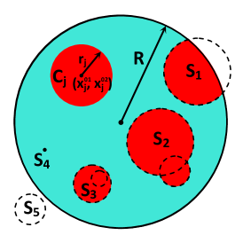
Figure 1: Different scenarios of $j$th circle appearance in the $i$th sample: regular case $C_{j}$ and special cases $S_{1}$ through $S_{5}$.

After completing the collection of $N$ sample solutions following the description above, the proposed computational algorithm for solving problem (5) could be executed in two steps:

• Define the initial basis of samples

  $$\mathcal{B}^{0}=(\bar{\sigma}_{i}(x))_{i=1}^{N_{s}}$$ (14)

  by choosing $N_{s}$ best samples out of collection $\mathcal{C}(N)$ which provide the best measurement fit in terms of cost functional (4).

• Set all parameters $(\mathcal{P}_{i})_{i=1}^{N_{s}}$ in the description of sample basis $\mathcal{B}$ as controls to perform optimization for solving problem (5) numerically to find the optimal basis $\hat{\mathcal{B}}$.

3.2 Step 1: Defining Initial Basis

This step requires solving forward problem (3) and evaluating cost functional (4) $N$ times for all samples in the $N$-collection. For a fixed scheme of potentials $U$ the data $\mathcal{D}_{i}=I^{k}_{\ell}(\sigma_{i})\in\mathbb{R}^{m^{2}},\ i=1,\ldots,N$, could be precomputed by (3) and (2) and then stored for multiple uses with different models. In addition, this task may be performed in parallel with minimal computational overhead which allows easy switching between various schemes for electrical potentials. Easy parallelization enables taking $N$ quite large which helps better approximate the solution by the initial state of basis $\mathcal{B}$ before proceeding to Step 2.

The number of samples $N_{s}$ in basis $\mathcal{B}$ may be defined experimentally based on the model complexity. We suggest $N_{s}$ to be sufficiently large to properly support a local/global search for optimal solution $\hat{\sigma}(x)$ during Step 2. At the same time this number should allow the total number of controls while solving problem (5) to be comparable with data dimension, namely $m^{2}$, for satisfying the well-posedness requirement.

Working with the models of complicated structures may require increasing the current number of elements (circles) in every sample within the chosen basis $\mathcal{B}$. In such a case, one could re-set parameters $N_{c}^{i},\ i=1,\ldots,N_{s}$, to higher values and add missing elements, for example, by generating new circles randomly as degenerate cases $S_{4}$. This will project the initial basis $\mathcal{B}^{0}$ onto a new control space of a higher dimension without any loses in the quality of the initial solution.

Step 1 will be completed after ranking samples in ascending order in terms of computed cost functionals (4) while comparing the obtained data $(\mathcal{D}_{i})_{i=1}^{N}$ with true data $(I_{\ell}^{k*})_{\ell,k=1}^{m}$ available from the actual measurements. After ranking, the first $N_{s}$ samples will create the initial basis $\mathcal{B}^{0}$ to be used in place of the initial guess for optimization in Step 2.

3.3 Step 2: Solving Optimal Control Problem

As discussed in Section 3.1, all elements (circles) in all samples of basis $\mathcal{B}$ obtained during Step 1 ranking procedure will be represented by a finite number of “sample-based” parameters $(\mathcal{P}_{i})_{i=1}^{N_{s}}$. In general, solution $\sigma(x)$ could be uniquely represented as a function of $\mathcal{P}_{i},\ i=1,\ldots,N_{s}$. The continuous form of optimal control problem (5) may be substituted with its new equivalent form defined over the finite set of controls $\mathcal{P}=(\mathcal{P}_{i})_{i=1}^{N_{s}}$. In addition to this, problem (5) could be further extended by adding weights $\alpha=(\alpha_{i})_{i=1}^{N_{s}}$ in (8) to the set of new controls. After this we arrive at the final form of the optimization problem to be later solved numerically:

$$(\hat{\mathcal{P}},\hat{\alpha})=\underset{\mathcal{P},\alpha}{\operatorname{argmin}}\ \mathcal{J}(\mathcal{P},\alpha)$$ (15)

subject to PDE constraint (3), linear constraint (9) and properly established bounds for all components of control $(\mathcal{P},\alpha)$. As easily followed from the structure of this new control, a dimension of the parameterized solution space is bounded by

$$\max(\dim(\mathcal{P},\alpha))=N_{s}\cdot[N_{c,\max}(n+1)+1].$$ (16)

When solving (15) iteratively, one may choose to terminate the optimization run at $k$th (major) iteration once the following criterion is satisfied:

$$\left|\dfrac{\mathcal{J}^{k}-\mathcal{J}^{k-1}}{\mathcal{J}^{k}}\right|<\epsilon$$ (17)

subject to chosen tolerance $\epsilon\in\mathbb{R}_{+}$. Although both (5) and (15) are obviously not separable optimization problems, the coordinate descent (CD) method is used to solve (15). This choice is motivated by several reasons, namely

• simplicity of the form for establishing the equivalence between controls $\sigma(x)$ and $(\mathcal{P},\alpha)$ provided by (8) and (11)–(12),

• close proximity of samples in the initial basis $\mathcal{B}^{0}$ to the local/global solutions after completing Step 1, and

• straightforward computational implementation.

The efficiency of the entire optimization framework is confirmed by extensive computational results for multiple models of different complexity presented in Section 4. A summary of the complete computational framework to perform our new optimization with sample-based parameterization is provided in Algorithm 1. We also note that in order to improve the computational efficiency, the applied CD method is modified by specifying the order in which all controls are perturbed while solving problem (15) as discussed in detail in Section 3.4. Briefly, instead of following the sensitivity feedback, choosing controls is considered in the sample-by-sample order, and within each sample $\bar{\sigma}_{i}$ we optimize over all circles’ triplets $\{x^{01}_{j},x^{02}_{j},r_{j}\}$ and then over the sample’s weight $\alpha_{i}$, see Step 2 in Algorithm 1 for clarity.

  set parameters: $N$, $N_{c,\max}$, $N_{s}$

  for $i\leftarrow 1$ to $N$ do

     generate $\bar{\sigma}_{i}(x)$ by (11)–(13)

     obtain data $\mathcal{D}_{i}=I^{k}_{\ell}(\bar{\sigma}_{i})$ by (3) and (2)

  end for

   Step 1 Defining Initial Basis

  select model and obtain true data $(I_{\ell}^{k*})_{\ell,k=1}^{m}$

  for $i\leftarrow 1$ to $N$ do

     compute $\mathcal{J}(\bar{\sigma}_{i})$ by (4)

  end for

  choose $N_{s}$ best samples from $\mathcal{C}(N)$ by values $\mathcal{J}(\bar{\sigma}_{i})$

  form initial basis $\mathcal{B}^{0}$ subject to $N_{c,\max}$

  set initial weights $\alpha^{0}$

  compute $\sigma^{0}(x)$ using $\mathcal{B}^{0}$ and $\alpha^{0}$ by (8)

   Step 2 Solving Optimal Control Problem

  $k\leftarrow 0$

  repeat

     for $i\leftarrow 1$ to $N_{s}$ do

        for $j\leftarrow 1$ to $N^{i}_{c}$ do

           optimize over $j$th circle triplet $\{x^{01}_{j},x^{02}_{j},r_{j}\}$ in $\bar{\sigma}_{i}$

        end for

        optimize over weight $\alpha_{i}$

     end for

     $k\leftarrow k+1$

     update $\sigma^{k}(x)$ using new basis $\mathcal{B}^{k}$ and weights $\alpha^{k}$ by (8)

  until termination criterion (17) is satisfied to given tolerance

Algorithm 1 Computational workflow for optimization with sample-based parameterized controls

3.4 Customized Coordinate Descent Method

To conclude on the practical implementation of our modified coordinate descent approach, customarily adopted for the proposed optimization framework, here we discuss some details. We also note that, despite the superior performance of the CD approach, its current version used for all computations in this paper still has enough room for further improvements towards computational efficiency and applicability for 2D and 3D problems.

After finishing Step 1 (refer to Section 3.2 for details), we then have a multitude of potential methods for performing optimization at Step 2 (see Section 3.3). As mentioned before, our preferred method is a customized version of the CD algorithm. Coordinate descent, or alternating variables, algorithms are a form of discrete gradient algorithms that determine if there is an apparent gradient by comparing the difference between the values of the cost functional when measured at two or more positions in the related domains, see [25] for more details. Gradient descent is then simulated by moving in discrete intervals, rather than a distance proportionate to the estimated gradient’s size as is common with typical gradient descent techniques.

In our algorithm, we start with initializing controls obtained from $N_{s}$ samples in use, namely all parameters $(\mathcal{P}_{i})_{i=1}^{N_{s}}$ from the initial basis $\mathcal{B}^{0}=(\bar{\sigma}^{0}_{i}(x))_{i=1}^{N_{s}}$ and associated weights $(\alpha^{0}_{i})_{i=1}^{N_{s}}$. We note that $\mathcal{B}^{0}$ and $\alpha^{0}$ are used to compute $\sigma^{0}(x)$, and the composite sample (image) to represent the final solution for Step 1 and simultaneously the initial guess used in Step 2.

The optimization process by the CD approach at Step 2 chooses controls one-by-one from the entire control space

$$(\mathcal{P},\alpha)=\{(\mathcal{P}_{i})_{i=1}^{N_{s}}\cup(\alpha_{i})_{i=1}^{N_{s}}\}$$ (18)

in the sample–by–sample order and circle-by-circle order within a sample. The ordered circles in all samples are sequentially moved horizontally, then vertically and finally resized by changing their radii. After completing the optimization over all circles in the $i$th sample, its weight $\alpha_{i}$ is also optimized to employ the benefits of the updated geometry of the current sample.

Now we focus on a single (minor) optimization iteration within this procedure for changing a single control $\zeta$ selected from $(\mathcal{P},\alpha)$. A summary for all steps within this iteration is provided in Algorithm 2.

  choose control $\zeta\in\{(\mathcal{P}_{i})_{i=1}^{N_{s}}\cup(\alpha_{i})_{i=1}^{N_{s}}\}$

  compute $\mathcal{J}_{curr}(\bar{\sigma}_{i})$ by (4)

  $d\leftarrow 1$

  $s\leftarrow 0$

  repeat

     if $d>0$ then

        increment $\zeta$ by (19) or (20)–(21)

     else

        decrement $\zeta$ by (19) or (20)–(21)

     end if

     compute $\mathcal{J}_{temp}(\bar{\sigma}_{i})$ by (4)

     if $\mathcal{J}_{curr}\leq\mathcal{J}_{temp}$ then

        if s = 0 then

           $d\leftarrow-1$

           decrement $\zeta$ by (19) or (20)–(21)

           $\mathcal{J}_{temp}\leftarrow\mathcal{J}_{curr}$

        end if

        $s\leftarrow s+1$

        if $s=s_{\max}$ then

           break

        end if

     else

        $s\leftarrow 1$

     end if

  until $\mathcal{J}_{curr}<\mathcal{J}_{temp}$

Algorithm 2 CD method: minor iteration

First, we choose a single parameter $\zeta$, for example, from the set of controls $\mathcal{P}$, as the current control variable and perturb it by a preset value, say constant step-size $\gamma$:

$$\zeta^{new}=\zeta^{old}\pm\gamma,\qquad\zeta\in(\mathcal{P}_{i})_{i=1}^{N_{s}}.$$ (19)

Then we determine if the cost functional $\mathcal{J}(\bar{\sigma})$ of the altered composite sample $\bar{\sigma}(x)$ improves (decreases) or worsens (increases). We always perturb the control $\zeta$ in the same direction along the given axis initially and then, depending upon if the cost functional improves or not, we decide how to proceed. If the cost functional improves, we perturb it in the same direction again and continue in that direction until we see an increase in the functional value. At this point, we select the best position found and move to the next control. If the initial perturbation worsens the functional, we then reverse direction along the given axis and continue in the same manner as before until we reach a point at which the cost functional worsens.

Perturbations in both directions may result in a position/radius associated with the cost functional value which is worse than its value computed at the initial position/radius. In this case, we revert to the parameter’s initial value and continue to the next parameter (control variable). If there is no change in the functional value, we continue in the same direction until there is either a change in the functional or some pre-specified amount of steps $s_{max}$ is reached, at which point the same behavior as described before is continued or we move to the first position that had the same functional value, respectively.

We perform a highly similar process when optimizing over the weights of each sample image in the composite, $\zeta\in\alpha$, but with a key difference. Being that instead of perturbing $\zeta=\alpha_{i}$ by some $\gamma$ value, we multiply the weight $\alpha_{i}$ by $1\pm\gamma$, i.e.

$$\zeta^{new}=(1\pm\gamma)\,\zeta^{old},\qquad\zeta\in(\alpha_{i})_{i=1}^{N_{s}},$$ (20)

and then normalize all weights subject to the convexity condition (9):

$$\alpha_{i}^{new}=\dfrac{\alpha_{i}^{old}}{1\pm\gamma\zeta^{old}},\qquad i=1,\ldots,N_{s}.$$ (21)

We would like to conclude on our modified CD approach by re-iterating that all operations across the controls are performed following the specific “schedule”. We start with the first circle in the description of the best matching sample identified during the Step 1 procedure. Then we proceed towards each consecutive control in this sample, namely $x^{01}_{1j}$ followed by $x^{02}_{1j}$ followed by $r_{1j}$, $j=1,\ldots,N_{c}^{i}$, until every parameter is optimized at which point the weight $\alpha_{1}$ for that sample is optimized. Then we proceed to the next sample, $i=2,3,\ldots,N_{s}$, and do the same. Once all $N_{s}$ samples have been optimized, we loop back to the first sample image and perform the same operations again and continue this process until at least one of the termination criteria is met.

4 Computational Results

4.1 Computational Model in 2D

Our optimization framework integrates computational facilities for solving forward PDE problem (3) and evaluating cost functionals by (4). These facilities are incorporated by using FreeFem++, see [19] for details, an open-source, high-level integrated development environment for obtaining numerical solutions of PDEs based on the finite element nethod (FEM). For solving numerically forward PDE problem (3), spatial discretization is carried out by implementing 7730 FEM triangular finite elements: P2 piecewise quadratic (continuous) representation for electrical potential $u(x)$ and P0 piecewise constant representation for conductivity field $\sigma(x)$. Systems of algebraic equations obtained after such discretization are solved with UMFPACK, a solver for nonsymmetric sparse linear systems [15].

All computations are performed using a 2D domain (6) which is a disc of radius $R=0.1$ with $m=16$ equidistant electrodes $E_{\ell}$ with half-width $w=0.12$ rad covering approximately 61% of boundary $\partial\Omega$ as shown in Figure 2(a). Electrical potentials $U_{\ell}$, see Figure 2(b), are applied to electrodes $E_{\ell}$ following the “rotation scheme” discussed in Section 2 and chosen to be consistent with the ground potential condition (1). Determining the Robin part of the boundary conditions in (3c), we equally set the electrode contact impedance $Z_{\ell}=0.1$. To solve optimal control problem (15) iteratively, our framework is utilizing derivative-free Coordinate Descent or alternating variables approach, see [25] for more details. The actual (true) electrical conductivity $\sigma_{true}(x)$ we seek to reconstruct is defined analytically for each model in (7) by setting $\sigma_{d}=0.4$ and $\sigma_{n}=0.2$. The initial guess for control $\mathcal{P}$ at Step 2 is provided by the parameterization of initial basis $\mathcal{B}^{0}$ obtained after completion of Step 1. For control $\alpha$, the initial values are set to be equal, i.e., $\alpha^{0}_{i}=1/N_{s}$. Termination criteria are set by tolerance $\epsilon=10^{-4}$ in (17) and the total number of cost functional evaluations 50,000 whichever is reached first.

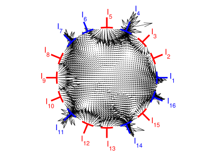
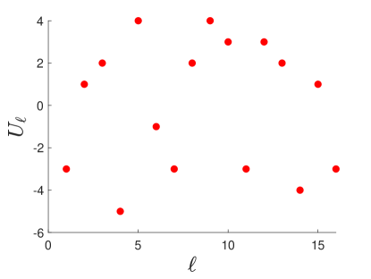
Figure 2: (a) Equispaced geometry of electrodes $(E_{\ell})_{\ell=1}^{16}$ and electrical currents $I_{\ell}$ (positive in red, negative in blue) measured at $E_{\ell}$. Black arrows show the distribution of flux $\sigma(x)\bm{\nabla}u(x)$ in the interior of $\Omega$. (b) Electrical potentials $U_{\ell}$.

For generating $N$-collection of samples discussed in Section 3.1 we use $N=10000$ and $N_{c,max}=8$. The set of sample solutions $\mathcal{C}(10000)$ is pre-computed using a generator of uniformly distributed random numbers. Therefore, each sample $\bar{\sigma}_{i}(x)$ “contains” from one to eight “defective” areas with $\sigma_{d}=0.4$. Each area is located randomly within domain $\Omega$ and represented by a circle of randomly chosen radius $0<r\leq 0.3R$. Also, we fix the number of samples $N_{s}$ to 10 for all numerical experiments shown in this paper, see [5] for more details. The entire preparation stage also involves computations for electrical currents (measurements) using (2)–(3) one time per sample solution with total computing time equivalent roughly to 10,000 cost functional evaluations. For example, this phase is completed in 10.3 h on a computer with a 26-core Intel Xeon Cascade Lake Refresh Gold 6230R processor running at 2.1 GHz using 256 GB of RAM under MS Windows Server 2019 by utilizing only one core. As all samples are independent of each other, the associated computations are highly parallelizable; this adds more to the computational efficiency of our new approach.

4.2 Framework Validation

To begin checking the performance of the proposed optimization framework, we created our (benchmark) model #1 to mimic a case when a medium contains three areas of different sizes and circular shapes to appear defective as seen in Figure 3(a). To prove the superior performance of the proposed algorithm supplied with the customized CD method for optimization, we refer first to Figure 3(b,c). The center image (b) shows the best, in terms of the measurement fit, sample solution found in the collection $\mathcal{C}(10000)$ for model #1 and placed into the initial basis $\mathcal{B}^{0}$ as $\bar{\sigma}_{1}(x)$. The right image (c) shows the solution $\sigma^{0}(x)$ obtained after Step 1 optimization procedure. Next, Figure 4(a,b) depicts the solutions obtained after Step 2 respectively with no circles and after adding new ones to each sample. It is noticeable that the structure of the best sample solution $\bar{\sigma}_{1}(x)$ is very far from $\sigma_{true}(x)$, and $\sigma^{0}(x)$, derived from the initial basis $\mathcal{B}^{0}$, poorly approximates model #1. However, the proposed sample-based parameterization enables the framework to accurately locate all defective regions, including the smallest one. As the next step, we investigate the effect of re-setting parameters $N_{c}^{i}$ as discussed in Section 3.2. Figure 4(c) shows the progress during Step 1 (first 10 major iterations, in pink) and Step 2 with no circles added (in blue) and after adding new circles to each sample (in red) so that $N_{c}^{i}=8,\ i=1,\ldots,10$. An interesting observation could be made from Figure 4(d,e) presenting the history of control $\alpha$ changes during Step 2 optimization. The comparison reveals more sensitivity (wider oscillation spans for all $\alpha$’s) in the second case related to the increased size of control space $\mathcal{P}$. Due to obviously better performance for that case, we use the same strategy, by setting $N_{c}^{i}=N_{c,max}$, in all numerical experiments presented in this paper unless otherwise stated.

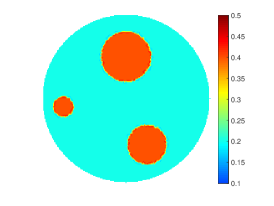
(a) model #1: $\sigma_{true}(x)$

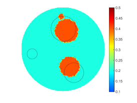
(b) best sample $\bar{\sigma}_{1}(x)$

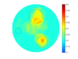
(c) solution $\sigma^{0}(x)$ after Step 1

Figure 3: Model #1. (a) True electrical conductivity $\sigma_{true}(x)$. Solutions by (b) best sample $\bar{\sigma}_{1}(x)$ from initial basis $\mathcal{B}^{0}$, and (c) complete initial basis $\mathcal{B}^{0}$ approximation $\sigma^{0}(x)$ obtained after Step 1.

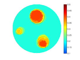
(a) $\hat{\sigma}(x)$: no circles added

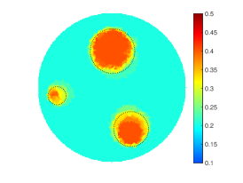
(b) $\hat{\sigma}(x)$: 8 circles/sample

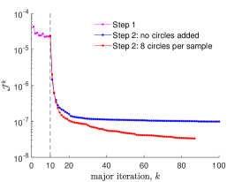
(c) effect of re-setting $N_{c}^{i}$

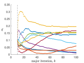
(d) $\alpha$: no circles added

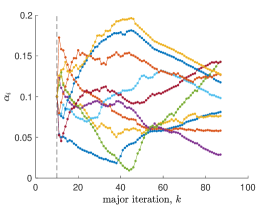
(e) $\alpha$: 8 circles/sample

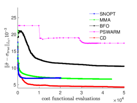
(f) solution error

Figure 4: Model #1. (a,b) Solution images after Step 2 with (d,e) history of control $\alpha$ changes for cases with (a,d) no circles added and (b,e) after adding new circles to each sample enforcing $N_{c}^{i}=8$. (c) Cost functionals $\mathcal{J}^{k}$ as a function of major iteration count $k$ evaluated at Step 1 (pink dots) and Step 2 with no circles added to samples (blue dots) and 8 circles per sample (red dots). (f) Solution error $\|\hat{\sigma}-\sigma_{true}\|_{L_{2}}$ as a function of number of cost functional evaluations for results obtained by gradient-based SNOPT (blue) and MMA (green), derivative-free BFO (black) and PSWARM (pink) all using PCA compared with CD (red) method with enforced $N_{c}^{i}=8$ condition.

We also use model #1 to compare the performance of the proposed framework with those observed after applying various methods, namely

• gradient-based sequential quadratic and sequential convex programming algorithms by, respectively, Sparse Nonlinear OPTimizer (SNOPT) [17] and method of moving asymptotes (MMA) [30],

• derivative-free brute force optimization (BFO) method from the BFO 2.0 package [27, 26] and the dual pattern and particle swarm algorithm Particle SWARM (PSWARM) [32] implemented through the OPTI Toolbox for nonlinear optimization problems [14] and

• our CD method customized to a predefined order of controls as described in Section 3.

To compare the quality of the obtained solutions both gradient-based and derivative-free methods (excluding our CD algorithm) are supplied with principal component analysis (PCA) techniques for control space reduction as described in detail in [22, 10, 33]. The PCA is performed on the same collection of samples $\mathcal{C}(10000)$ and with the same number of principal components, 250 (preserving about 90% of the “energy” in the full set of basis vectors), as the total number of controls used in the CD method.

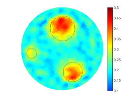
(a) $\hat{\sigma}(x)$ by SNOPT

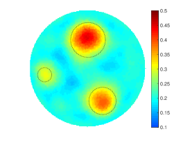
(b) $\hat{\sigma}(x)$ by MMA

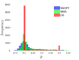
(c) $\hat{\sigma}(x)$ distribution

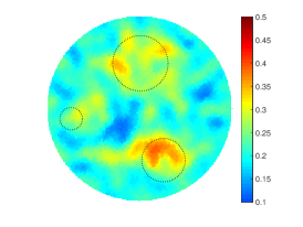
(d) $\hat{\sigma}(x)$ by BFO

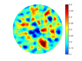
(e) $\hat{\sigma}(x)$ by PSWARM

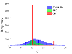
(f) $\hat{\sigma}(x)$ distribution

Figure 5: Model #1. (a,b,d,e) Solutions images obtained by (a) SNOPT, (b) MMA, (d) BFO, and (e) PSWARM. (c,f) Histograms for solutions obtained by (c) SNOPT and MMA, (f) BFO and PSWARM compared with the CD method.

Figure 5(a,b,d,e) shows the images obtained, respectively, by SNOPT, MMA, BFO, and PSWARM approaches with combined accuracy results provided in Figure 4(f). To make the superior performance of the proposed customized CD method even more distinctive, all four approaches used termination tolerance $\epsilon=10^{-9}$ in contrast to $10^{-4}$ in the CD’s case. As seen in Figure 4(f), in general, gradient-based approaches are able to provide images of better qualities. Both derivative-free approaches, as expected, showed much slower convergence terminated when the total number of cost functional evaluations reached 50,000. Although our derivative-free CD approach is also terminated with the same condition, it arrives at a solution with better quality than is seen in the gradient-based methods. To add more, only our new CD method results in quality close to the desired binary distribution (refer to Figure 5(c,f) for analysis by histograms).

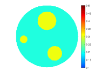
(a) $\sigma_{true}(x),\sigma_{d}=0.3$

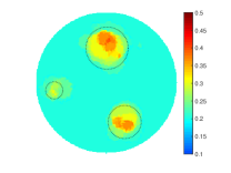
(b) $\hat{\sigma}(x),\sigma_{d}=0.3$

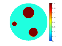
(c) $\sigma_{true}(x),\sigma_{d}=0.5$

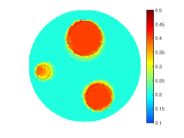
(d) $\hat{\sigma}(x),\sigma_{d}=0.5$

Figure 6: Model #1. (a,c) True electrical conductivity $\sigma_{true}(x)$ and (b,d) respective solution images obtained by the derivative-free customized CD method when (a,b) $\sigma_{d}=0.3$ and (c,d) $\sigma_{d}=0.5$.

Finally, we would like to address the issue of a priori knowledge of $\sigma_{d}$ and $\sigma_{n}$ used in (11) as approximations for conductivities, respectively, of defective region $\Omega_{d}$ and the rest of the domain $\Omega_{n}$. The solution formulation given by (8) suggests that values $\sigma_{d}$ and $\sigma_{n}$ in (7) may vary from those used in the sampling procedure by (11). We check this ability for reconstructing different conductivity values by running two numerical experiments where $\sigma_{d}$ is set to 0.3 and 0.5 (instead of 0.4 used before). Figure 6 presents the results from both cases proving the method’s ability to detect the inclusions accurately. Further comparison of images in Figures 6(b,d) and 4(b) (varied vs. predefined conductivity) reveals the difference in the $\sigma$-values within the defective regions and suggests the suitability of the proposed methodology for quantitative imaging. The entire computational framework may be further modified to allow both $\sigma_{d}$ and $\sigma_{n}$ to be randomly chosen at the expense of enlarging the control space. It may require adding gradients combined with the derivative-free approach considered in this paper to keep the method computationally efficient.

4.3 Effect of Noise in Data

Now we would like to address a well-known issue of the noise present in the measurements due to improper electrode-medium contacts, possible electrode misplacement, wire interference, etc. The effect of noise has already been investigated by many researchers both theoretically and within practical applications with suggested approaches to mitigate its negative impact on the quality of images. In this section, we compare the effect of noise in reconstructions obtained by the gradient-based SNOPT and MMA (both with PCA) and our proposed derivative-free customized CD method.

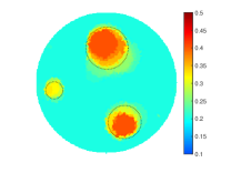
(a) CD: 0.5% noise

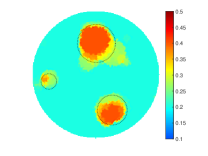
(b) 1% noise

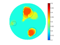
(c) 2% noise

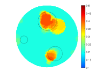
(d) 5% noise

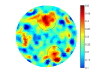
(e) SNOPT: 0.5% noise

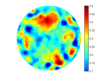
(f) 1% noise

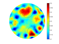
(g) 2% noise

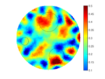
(h) 5% noise

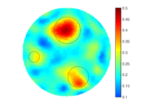
(i) MMA: 0.5% noise

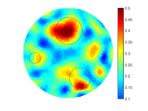
(j) 1% noise

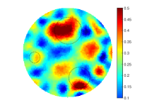
(k) 2% noise

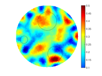
(l) 5% noise

Figure 7: Model #1. Solution images obtained by (a-d) the proposed derivative-free customized CD, gradient-based (e-h) SNOPT, and (i-l) MMA methods when measurements are contaminated with (a,e,i) 0.5%, (b,f,j) 1%, (c,g,k) 2%, and (d,h,l) 5% noise.

In Figure 7, we revisit model #1 presented first in Section 4.2 now with measurements contaminated with 0.5%, 1%, 2% and 5% normally distributed noise. As expected, we see that various levels of noise lead to oscillatory instabilities in the images reconstructed by the gradient-based approaches utilizing parameterization via PCA. This will obviously result in multiple cases of false positive outcomes in screening procedures. On the other hand, our new approach with sample-based parameterization shows its stable ability to provide clear and accurate images with the appearance of false negative results for small regions only with noise higher than 2%. Figure 8 provides the complete comparison of the solution error for results obtained by our framework for various levels of noise between 0% and 5%. We close this section by concluding on using 0.5% noise for the rest of the numerical experiments shown in this paper.

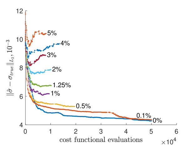
Figure 8: Model #1. Solution error $\|\hat{\sigma}-\sigma_{true}\|_{L_{2}}$ as a function of the number of cost functional evaluations for results obtained by the proposed framework for various levels of noise.

4.4 Validation with Complicated Models

In this section, we present results obtained using our new optimization framework with sample-based parameterization applied to models with a significantly increased level of complexity. The new algorithm has already confirmed its ability to reconstruct accurately defective regions of various size and at multiple locations. Therefore, the added complications we are focusing on here are of small sizes and non-circular shapes for those regions.

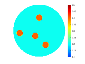
(a) model #2: $\sigma_{true}(x)$

(b) CD: no noise

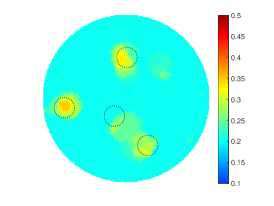
(c) CD: 0.5% noise

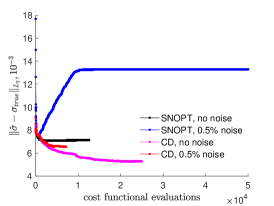
(d) solution error

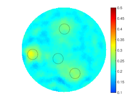
(e) SNOPT: no noise

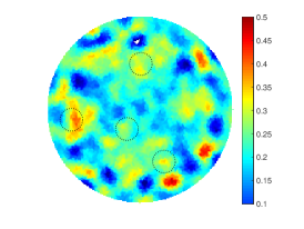
(f) SNOPT: 0.5% noise

Figure 9: Model #2. (a) True electrical conductivity $\sigma_{true}(x)$. (b,c,e,f) Solution images obtained by (b,c) the proposed framework and (e,f) the gradient-based SNOPT with PCA with (b,e) no noise added and (c,f) 0.5% noise in measurements. (d) Solution error $\|\hat{\sigma}-\sigma_{true}\|_{L_{2}}$ as a function of the number of cost functional evaluations for images shown in (b,c,e,f).

Our model #2 is created to check the ability of the EIT techniques coupled with our new approach to find the inclusions (defects) of very small sizes. It mimics, for example, the application of EIT in medical practice for recognizing cancer at early stages. The systematic analysis on the distinguishability of two different conductivity distributions with a specified precision is provided in [21]. The electrical conductivity $\sigma_{true}(x)$ is shown in Figure 9(a). This model contains four circular-shaped defective regions all of the same size as the smallest region in model #1. The known complication comes from the fact that the order of difference in measurements generated by this model and “fully normal medium” ($\sigma(x)=\sigma_{n},\ \forall x\in\Omega$) is very close to the order of noise that appears naturally in the provided data. In addition to this, small regions have a lower chance of being detected if they are located closer to the center of the domain.

Figure 9(b-f) compares the results obtained by the gradient-based SNOPT with PCA and our proposed derivative-free customized CD methods without noise and with 0.5% noise added to the measurements. By analyzing images in Figure 9, we see that our approach is able to provide more assistance in concluding on possible defects in medium and help navigate for their search. When noise is negligible, Figure 9(b), all four small spots are distinguishable with accurately reconstructed shapes. Although adding noise, as seen in Figure 9(c), brings more complexity to image interpretation, it still keeps the possibility to help identify defective regions. In fact we cannot claim the same for images obtained by means of PCA and gradients, see Figure 9(e,f). Figure 9(d) also proves computational efficiency of our framework in comparison with the gradient-based method.

Our last model #3, the hardest one, is created to check the method’s performance when the reconstructed region is not of a circular shape, see Figure 10(a) with a C-shape region. As seen in Figure 10(d), the gradient-based method with PCA is unable to get a clear image even without noise, as the PCA transform honors the structures of samples in the $\mathcal{C}(10000)$ collection. On the other hand, our new framework could provide a good quality image with no noise in the data. This performance may be further enhanced, even in the presence of noise, once we re-set the number of circles condition to $N_{c}^{i}=N_{c,max}=20$. This proves the potential of the proposed algorithm in applications with rather complex models.

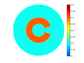
(a) model #3: $\sigma_{true}(x)$

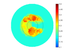
(b) CD: 8 circles, no noise

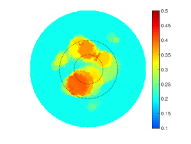
(c) CD: 8 circles, 0.5% noise

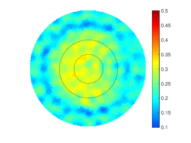
(d) SNOPT: no noise

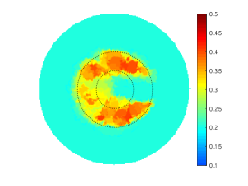
(e) CD: 20 circles, no noise

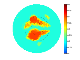
(f) CD: 20 circles, 0.5% noise

Figure 10: Model #3. (a) True electrical conductivity $\sigma_{true}(x)$. (b-f) Solution images obtained by (b,c,e,f) the proposed framework and (d) the gradient-based SNOPT with PCA with (b,d,e) no noise added and (c,f) 0.5% noise in measurements. Images in (b,c,e,f) are obtained by utilizing (b,c) $N_{c}^{i}=N_{c,max}=8$ and (e,f) $N_{c}^{i}=N_{c,max}=20$ conditions for the number of circles.

5 Concluding Remarks

In this work, we presented a novel computational approach for optimal reconstruction of binary-type images useful in various applications for (bio)medical practices. The proposed computational framework uses a derivative-free optimization algorithm supported by a set of sample solutions generated synthetically based on prior knowledge of the simulated phenomena. This framework has an easy-to-follow design tuned by a nominal number of computational parameters. High computational efficiency is achieved by applying the coordinate descent method customized to work with individual controls in the predefined custom order.

We investigated the performance of the complete framework in applications to the 2D IPCD by the EIT technique. We claim, based upon our results, that the proposed methodology of determining whether certain material or medium contains a defective region has superior efficiency in comparison with commonly used gradient-based and derivative-free techniques utilizing control space parameterization via PCA. It is due primarily to the predominately geometric nature of our approach, wherein we perturb known solutions to similar related problems in order to converge to the best available local/global minima.

There are many ways in which our proposed optimization framework can be further tested and extended. Among other directions, we see the greatest importance to test this approach in various applications to real data and different types of defects/abnormalities in the media, as this would certainly suggest new areas in which future developments may be required. Even though this computational approach is initially tested with synthetic EIT-related problems, we believe that this methodology could also be easily applied to a broad range of problems seen in various fields such as physics, geology, chemistry, etc.

References

- [1] Abascal, J.F.P.J., Lionheart, W.R.B., Arridge, S.R., Schweiger, M., Atkinson, D., Holder, D.S.: Electrical impedance tomography in anisotropic media with known eigenvectors. Inverse Problems 27(6), 1–17 (2011)
- [2] Abdulla, U.G., Bukshtynov, V., Seif, S.: Cancer detection through Electrical Impedance Tomography and optimal control theory: Theoretical and computational analysis. Mathematical Biosciences and Engineering 18(4), 4834–4859 (2021)
- [3] Adler, A., Arnold, J., Bayford, R., Borsic, A., Brown, B., Dixon, P., Faes, T.J., Frerichs, I., Gagnon, H., Gärber, Y., Grychtol, B., Hahn, G., Lionheart, W., Malik, A., Stocks, J., Tizzard, A., Weiler, N., Wolf, G.: GREIT: towards a consensus EIT algorithm for lung images. In: 9th EIT conference 2008, 16-18 June 2008, Dartmouth, New Hampshire. Citeseer (2008)
- [4] Adler, A., Gaburro, R., Lionheart, W.: Handbook of Mathematical Methods in Imaging, chap. Electrical Impedance Tomography, pp. 701–762. Springer New York, New York, NY (2015)
- [5] Arbic II, P.R.: Optimization Framework for Reconstructing Biomedical Images by Efficient Sample-based Parameterization. M.S. Thesis, Florida Institute of Technology, Scholarship Repository (2020). URL http://hdl.handle.net/11141/3220
- [6] Bera, T.K.: Applications of electrical impedance tomography (EIT): A short review. IOP Conference Series: Materials Science and Engineering 331, 012,004 (2018)
- [7] Borcea, L.: Electrical impedance tomography. Inverse Problems 18, 99–136 (2002)
- [8] Boverman, G., Kao, T.J., Kulkarni, R., Kim, B.S., Isaacson, D., Saulnier, G.J., Newell, J.C.: Robust linearized image reconstruction for multifrequency eit of the breast. IEEE Transactions on Medical Imaging 27(10), 1439–1448 (2008)
- [9] Brown, B.: Electrical impedance tomography (EIT): A review. Journal of Medical Engineering and Technology 27(3), 97–108 (2003)
- [10] Bukshtynov, V., Volkov, O., Durlofsky, L., Aziz, K.: Comprehensive framework for gradient-based optimization in closed-loop reservoir management. Computational Geosciences 19(4), 877–897 (2015)
- [11] Calderon, A.P.: On an inverse boundary value problem. In: Seminar on Numerical Analysis and Its Applications to Continuum Physics, pp. 65–73. Soc. Brasileira de Mathematica, Rio de Janeiro (1980)
- [12] Cheney, M., Isaacson, D., Newell, J.: Electrical impedance tomography. SIAM Review 41(1), 85–101 (1999)
- [13] Choi, M.H., Kao, T.J., Isaacson, D., Saulnier, G.J., Newell, J.C.: A reconstruction algorithm for breast cancer imaging with electrical impedance tomography in mammography geometry. IEEE Transactions on Biomedical Engineering 54(4), 700–710 (2007)
- [14] Currie, J., Wilson, D.I.: OPTI: lowering the barrier between open source optimizers and the industrial MATLAB user. In: N. Sahinidis, J. Pinto (eds.) Foundations of Computer-Aided Process Operations. Savannah, Georgia, USA (2012)
- [15] Davis, T.A.: Algorithm 832: UMFPACK V4.3 – an unsymmetric-pattern multifrontal method. ACM Transactions on Mathematical Software (TOMS) 30(2), 196–199 (2004)
- [16] Fan, Y., Ying, L.: Solving electrical impedance tomography with deep learning. Journal of Computational Physics 404, 109,119 (2020)
- [17] Gill, P., Murray, W., Saunders, M.: User’s Guide for SNOPT Version 7: Software for Large-Scale Nonlinear Programming. Stanford University (2008)
- [18] Hamilton, S.J., Hauptmann, A.: Deep d-bar: Real-time electrical impedance tomography imaging with deep neural networks. IEEE Transactions on Medical Imaging 37(10), 2367–2377 (2018)
- [19] Hecht, F.: New development in FreeFem++. Journal of Numerical Mathematics 20(3-4), 251–265 (2012)
- [20] Holder, D.S.: Electrical Impedance Tomography. Methods, History and Applications. CRC Press (2004)
- [21] Isaacson, D.: Distinguishability of conductivities by electric current computed tomography. IEEE Transactions on Medical Imaging 5(2), 91–95 (1986)
- [22] Koolman, P.M., Bukshtynov, V.: A multiscale optimization framework for reconstructing binary images using multilevel PCA-based control space reduction. Biomedical Physics & Engineering Express 7(2), 025,005 (2021)
- [23] Lionheart, W.: EIT reconstruction algorithms: Pitfalls, challenges and recent developments. Physiological Measurement 25(1), 125–142 (2004)
- [24] Liu, D., Du, J.: A moving morphable components based shape reconstruction framework for electrical impedance tomography. IEEE Transactions on Medical Imaging 38(12), 2937–2948 (2019)
- [25] Nocedal, J., Wright, S.J.: Numerical Optimization, 2nd edn. Springer (2006)
- [26] Porcelli, M., Toint, P.L.: Global and local information in structured derivative free optimization with BFO. arXiv:2001.04801
- [27] Porcelli, M., Toint, P.L.: BFO, a trainable derivative-free brute force optimizer for nonlinear bound-constrained optimization and equilibrium computations with continuous and discrete variables. ACM Trans. Math. Softw. 44(1) (2017)
- [28] Ren, S., Sun, K., Tan, C., Dong, F.: A two-stage deep learning method for robust shape reconstruction with electrical impedance tomography. IEEE Transactions on Instrumentation and Measurement 69(7), 4887–4897 (2020)
- [29] Somersalo, E., Cheney, M., Isaacson, D.: Existence and uniqueness for electrode models for electric current computed tomography. SIAM Journal on Applied Mathematics 52(4), 1023–1040 (1992)
- [30] Svanberg, K.: The method of moving asymptotes — a new method for structural optimization. International Journal for Numerical Methods in Engineering 24(2), 359–373 (1987)
- [31] Uhlmann, G.: Electrical impedance tomography and Calderón’s problem. Inverse Problems 25(12), 123,011 (2009)
- [32] Vaz, A.I.F., Vicente, L.N.: A particle swarm pattern search method for bound constrained global optimization. Journal of Global Optimization 39, 197–219 (2007)
- [33] Volkov, O., Bukshtynov, V., Durlofsky, L., Aziz, K.: Gradient-based Pareto optimal history matching for noisy data of multiple types. Computational Geosciences 22(6), 1465–1485 (2018)
- [34] Wang, Z., Yue, S., Wang, H., Yanqiu: Data preprocessing methods for electrical impedance tomography: a review. Physiological Measurement 41(9), 09TR02 (2020)
- [35] Wei, Z., Liu, D., Chen, X.: Dominant-current deep learning scheme for electrical impedance tomography. IEEE Transactions on Biomedical Engineering 66(9), 2546–2555 (2019)
- [36] Zou, Y., Guo, Z.: A review of electrical impedance techniques for breast cancer detection. Medical Engineering and Physics 25(2), 79–90 (2003)