Problems using deep generative models for probabilistic audio source separation

Abstract

Recent advancements in deep generative modeling make it possible to learn prior distributions from complex data that subsequently can be used for Bayesian inference. However, we find that distributions learned by deep generative models for audio signals do not exhibit the right properties that are necessary for tasks like audio source separation using a probabilistic approach. We observe that the learned prior distributions are either discriminative and extremely peaked or smooth and non-discriminative. We quantify this behavior for two types of deep generative models on two audio datasets.

1 Introduction: Langevin dynamics for source separation

Our initial goal was to use Langevin dynamics [11] in combination with deep generative priors to perform source separation of audio mixes. Our approach closely follows the work of [3], where mixed images are successfully separated. The biggest advantage of the approach used by [3] is that it does not rely on pairs of source signals and mixes as required by SOTA audio source separation models [10, 4]. Last, in contrast to [9], we are interested in performing the source separation in the time domain, which has multiple advantages like decreased computational complexity as well as the preservation of the phase of the signals. As common in the source separation literature, we assume that the mix $\boldsymbol{m}\in\mathcal{X}$ is a linear combination of $N$ source signals $\boldsymbol{s}_{1},\dots,\boldsymbol{s}_{N}\in\mathcal{X}$

$$\boldsymbol{m}=g(\boldsymbol{s})=\sum_{k=1}^{N}\alpha_{k}\boldsymbol{s}_{k}.$$ (1)

As seen in [3], we take a probabilistic approach in order to solve the source separation problem. According to Bayes rule we can compute the posterior distribution using

$$p(\boldsymbol{s}|\boldsymbol{m})=\frac{p(\boldsymbol{s})p(\boldsymbol{m}|\boldsymbol{s})}{p(\boldsymbol{m})},$$ (2)

where we use a Gaussian approximation $p(\boldsymbol{m})=\mathcal{N}(g(\boldsymbol{s}),\gamma^{2}I)$ with noise parameter $\gamma$. Stochastic Gradient Langevin Dynamics (SGLD) [21] enables us sample from the posterior distribution $p(\boldsymbol{s}|\boldsymbol{m})$ without the need for evaluating $p(\boldsymbol{m})$. A new sample of the source signals can be generated by

$$\boldsymbol{s}^{t+1}=\boldsymbol{s}^{t}+\eta\nabla_{\boldsymbol{s}}\left(\log p(\boldsymbol{s}^{t})+\frac{1}{2\gamma^{2}}\left\lVert\boldsymbol{m}-g(\boldsymbol{s}^{t})\right\rVert^{2}\right)+\sqrt{2\eta}\epsilon,$$ (3)

where $\epsilon=\mathcal{N}(0,1)$. Last, we assume that the prior of the source signals factorizes as follows

$$p(\boldsymbol{s})=p(\boldsymbol{s}_{1},\dots,\boldsymbol{s}_{N})=p(\boldsymbol{s}_{1})\dots p(\boldsymbol{s}_{N}).$$ (4)

We choose to parameterize the priors $p(\boldsymbol{s}_{1})\dots p(\boldsymbol{s}_{N})$ with deep generative models. This allows us to easily compute $\nabla_{\boldsymbol{s}}\log p(\boldsymbol{s}^{t})$ using the automatic differentiation tools from [12]. As noted in [3], in order to successfully recover the original source signals using Equation 3, we require the priors $p(\boldsymbol{s}_{1})\dots p(\boldsymbol{s}_{N})$ to be discriminative as well as sufficiently smooth. After our initial experiments failed, we observed that the learned prior distributions are either discriminative and extremely peaked or smooth and non-discriminative. In the following, we quantify this behavior for two types of deep generative models on two audio dataset.

2 Method: Modeling raw audio with generative models

Deep learning models as used for image applications are unsuitable for raw audio signals (signals in the time-domain). Digital audio is sampled at high sample rates, commonly 16kHz up to 44kHz. The features of interest lie at scales of strongly different magnitudes. Therefore, generative models need to model the complete range of frequencies containing high-frequency features like timbre and slow frequency features like song structure. We will be using two types of generative models to learn the likelihood $p(\boldsymbol{s})$ of audio signals, namely, WaveNet [18] and FloWaveNet [5].

WaveNet

The WaveNet is an autoregressive generative model for raw audio. The generation of a new sample $x_{t}$ is conditioned on all previous samples $x_{1},\dots,x_{t-1}$. The likelihood of the entire signal is given by

$$p(\boldsymbol{x})=\prod_{t=1}^{T}p(x_{t}|x_{1},\dots,x_{t-1}).$$ (5)

After training, starting from a single sample the model is able to iteratively generate a coherent time signal. The distribution $p(x_{t}|x_{1},\dots,x_{t-1})$ is modeled as a multinomial logistic regression, therefore the continuous signal $x$ is discretized using a so-called $\mu$-law encoding [18], resulting in 256 classes. Due to the autoregressive nature of the Wavenet the genrative process is diffiult to parallalize and generally slow.

The WaveNet adapts the PixelCNN [19] architecture to the audio domain. It is a fully-convolutional network where dilated causal convolutions [23] are used. Using a stack of dilated convolutions increases the receptive field of the deep features without increasing the computational complexity. Further, the convolutions are gated [2] and the output is constructed as the sum of skip connections from each layer. The skip connections fuse information from multiple time-scales.

FloWaveNet

An alternative to using an autoregressive model to model $p(\boldsymbol{x})$ are normalizing flows [15]. Normalizing flows are a class of exact likelihood models, which are amenable to gradient-based optimisation and efficient in inference and sampling. A standard normalizing flow in continuous space, is based on the simple change of variables formula. Given an observed data variable $\boldsymbol{x}\in X$; a prior probability distribution $p_{Z}(\cdot)$ on a latent variable $\boldsymbol{z}\in Z$, and a differentiable, bijective function $\boldsymbol{z}=f(\boldsymbol{x})$, we can model a probability distribution $p_{X}({\boldsymbol{x}})$ as

$$p_{X}(\boldsymbol{x}) =p_{Z}(f(\boldsymbol{x}))\bigg{\lvert}\det\bigg{(}\frac{\partial f(\boldsymbol{x})}{\partial\boldsymbol{x}}\bigg{)}\bigg{\rvert}.$$ (6)

Since Equation 6 requires the computation of a determinant, a special architecture is necessary to reduce the computational cost. One such architecture was introduced in [1]. [1] is using so-called coupling layers in which an input $\boldsymbol{x}$ is masked into two equally sized parts $\boldsymbol{x}_{a}$ and $\boldsymbol{x}_{b}$. One part is fed into a function to provide the weights of an affine transformation ($s(\cdot),t(\cdot)$) of the other

$$\hat{\boldsymbol{x}}_{b}=s(\boldsymbol{x}_{a})\cdot\boldsymbol{x}_{b}+t(\boldsymbol{x}_{a}).$$ (7)

The resulting Jacobian is a triangular matrix, whose determinant can be easily computed. There exist multiple approaches to combine the dilated convolutions used in the WaveNet and normalizing flows. In the case of FloWaveNet  [5] a WaveNet encoder is used to predict the weights of the affine transformation within every coupling layer. This architecture enables fast, parallel generation of audio samples.

3 Experiments

3.1 Datasets

Figure 1: One period of each of the four toy waveforms: sine, sawtooth, square and triangle wave.

Figure 2: The four source channels for the musdb18 dataset: bass ,drums, vocals and other.

Toy data

We create a toy-like dataset consisting of four distinct waveforms, as shown in Figure 2: a sine, a sawtooth, a square and a triangle wave. We generate the waveforms using a sampling frequency of $16$\mathrm{kHz}$$. For each waveform we sample a random frequency $f\in[27$\mathrm{Hz}$,4186$\mathrm{Hz}$]$, a random amplitude $A\in[0.8,1.0]$ and a random phase $\phi\in[0,2\pi]$.

$$\boldsymbol{m}=\frac{1}{4}\sum_{i}^{4}\boldsymbol{s}_{i}$$ (8)

The mix $\boldsymbol{m}$ is equal to the mean of the four source signals. We create 5000 mixes of one second length for training and a testset of 1500 mixes.

musdb18

The musdb18 [13] dataset, created for the 2018 Signal Separation Evaluation Campaign [16], is a benchmark dataset used to evaluate audio source separation algorithms. The dataset consists of 150 songs from various artists and genres, split into train and test sets sized 100 and 50, respectively. For each song, the full mix $\boldsymbol{m}$ and four separate sources $\boldsymbol{s}_{1},\boldsymbol{s}_{2},\boldsymbol{s}_{3},\boldsymbol{s}_{4}$ are given: drums, bass, vocals and others. The others source contains any instruments not contained in the first three. Note that the mix $\boldsymbol{m}$ does not strictly follow Equation 8 since it involves audio effects like compression. The song files are encoded with a sampling rate of $44.1$\mathrm{kHz}$$ which we down-sample to $16$\mathrm{kHz}$$. We extract 150 fixed-length frames of one second from each song.

3.2 Discrimative power of the priors

(a) FloWaveNet

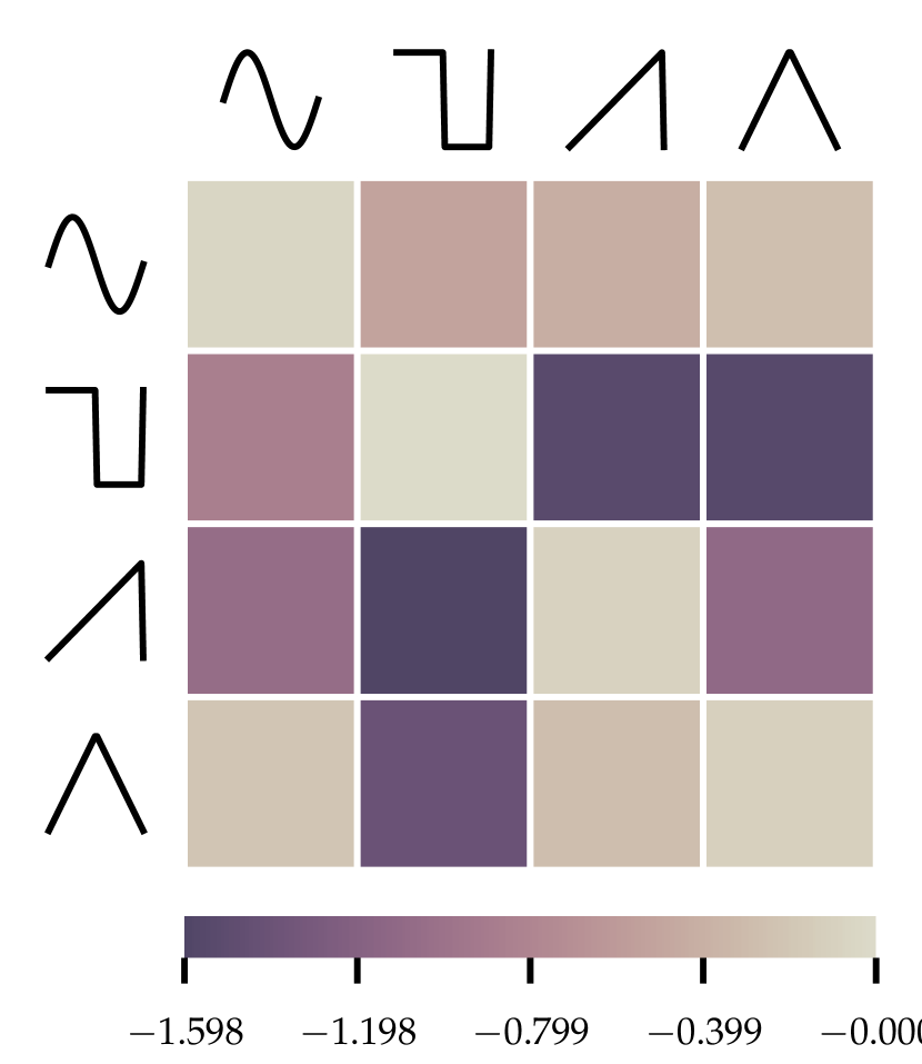
(b) WaveNet

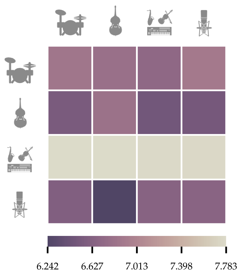
(c) FloWaveNet

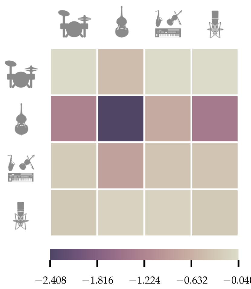
(d) WaveNet

Figure 3: The log-likelihood of each source under each prior for both sets of priors. Notice how for the Toy data we get the diagonal that we are expecting while for the real music the likelihood for every field is high and in the same range. The other prior assigns the highest likelihoods.

In the following, we train a separate WaveNet and FloWaveNet model for each signal source type of both datasets, in total eight separate generative models for each dataset. Details about architecture choices and training schedules can be found in the Appendix 5.

Using Langevin dynamics for separation we optimize the separated source frames under each prior model. During training of the deep generative priors, they explicitly contract the density for positive, in-class examples. During separation, the priors encounter negative out-of-distribution samples for the first time. To be useful for separation, the priors have to give a low likelihood to samples from the other possible sources.

Following the results in [8], we test the out-of-distribution detection performance of the deep generative priors by evaluating the mean log-likelihood of the test data of each source under each source prior. In Figure 3 we show that only for the FloWaveNet model trained with the Toy data behaves as anticipated. The in-class samples have a high likelihood while for all prior models the out-of-class samples have a low likelihood.

For the musdb18 dataset, neither the WaveNet- nor the FloWaveNet-based priors can discriminate between in-class and out-of-class samples. We hypothesize that this stems from the fact that the real musical data is severely more complicated compared than the Toy data. The in-class variability of the real sources is that high, that the models are not able to learn a distribution that would be discriminative. Note that the source other in musdb18 contains an undefined set of instruments making a model of those sounds in general impractical. But even if we are ignoring this subset neither prior model can discriminate the remaining source types. As a result, for the following experiments we focus on the Toy data dataset.

3.3 Smoothness of the learned distribution

In the case of the Toy dataset, only the FloWaveNet priors can distinguish between in-class and out-of-class signals. However, when we tried to use those priors for source separation as described in Section 1, we failed. We argue that one possible explanation is the peakedness of the learned prior distributions. The probability mass learned by the model is peaked at true samples but quickly decays with more disturbance of the input. The reason for this behavior is that all models are trained with noise-free samples of their respective signal sources (sine, square, saw, triangle).

As proposed in [3], we now approximate the noisy distribution $\log p_{\sigma}(\bm{x})$, which is the convolution of the noiseless distribution with a Gaussian with variance $\sigma$: $\log p_{\sigma}(\bm{x})*\mathcal{N}(0,\sigma)$ by adding Gaussian noise with the same variance to the input. Figuratively speaking, the Gaussian noise in data space translates to Gaussian smoothing of the peak in the probability distribution of the data.

Instead of retraining the deep generative priors we fine-tune [22] the noise-free models used in Section 3.2. We follow [3] in evaluating the noise-conditional model at different levels of noise $\sigma\in\{0.01,0.027,0.077,0.129,0.359\}$. In Figure 4 we show the cross mean log-likelihood for increasing noise-conditionals for the Toy data dataset. We find that even with small levels of conditional noise added the discriminative power of the learned generative models decays significantly. While being smooth the noise-conditional distributions cannot be used for source separation as intended.

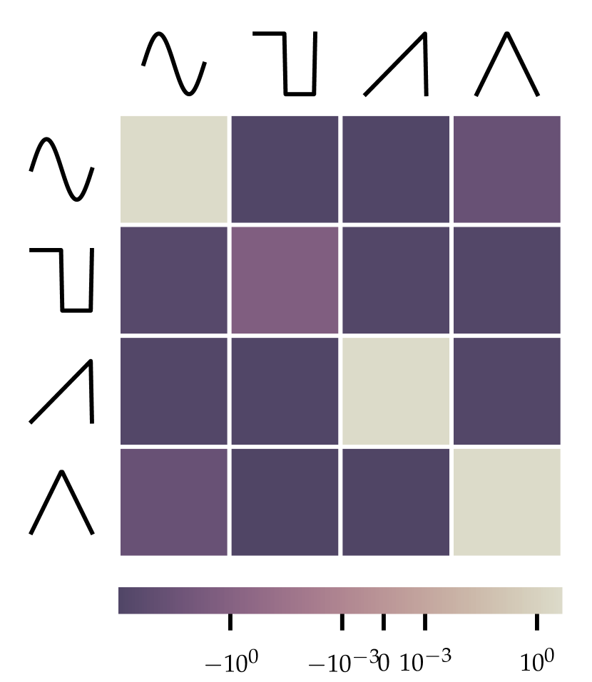
(a) $\sigma=0.0$

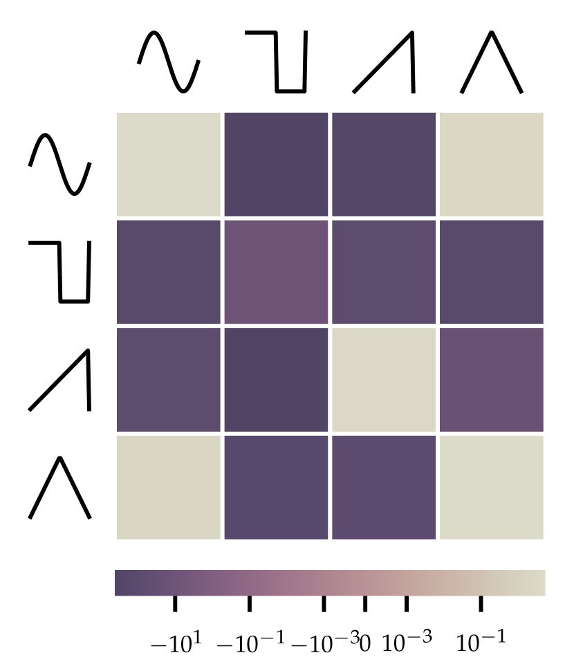
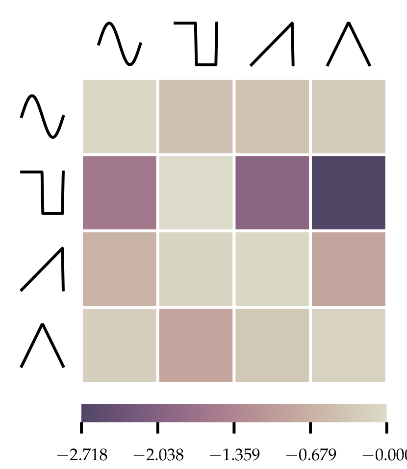
(b) $\sigma=0.01$

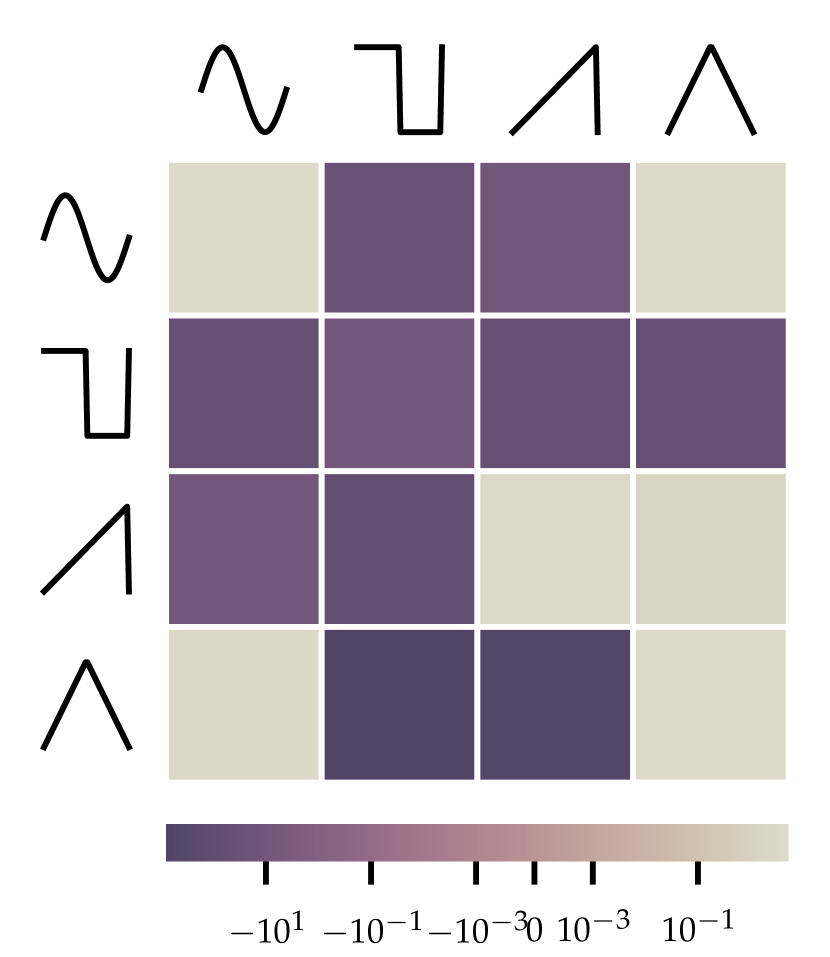
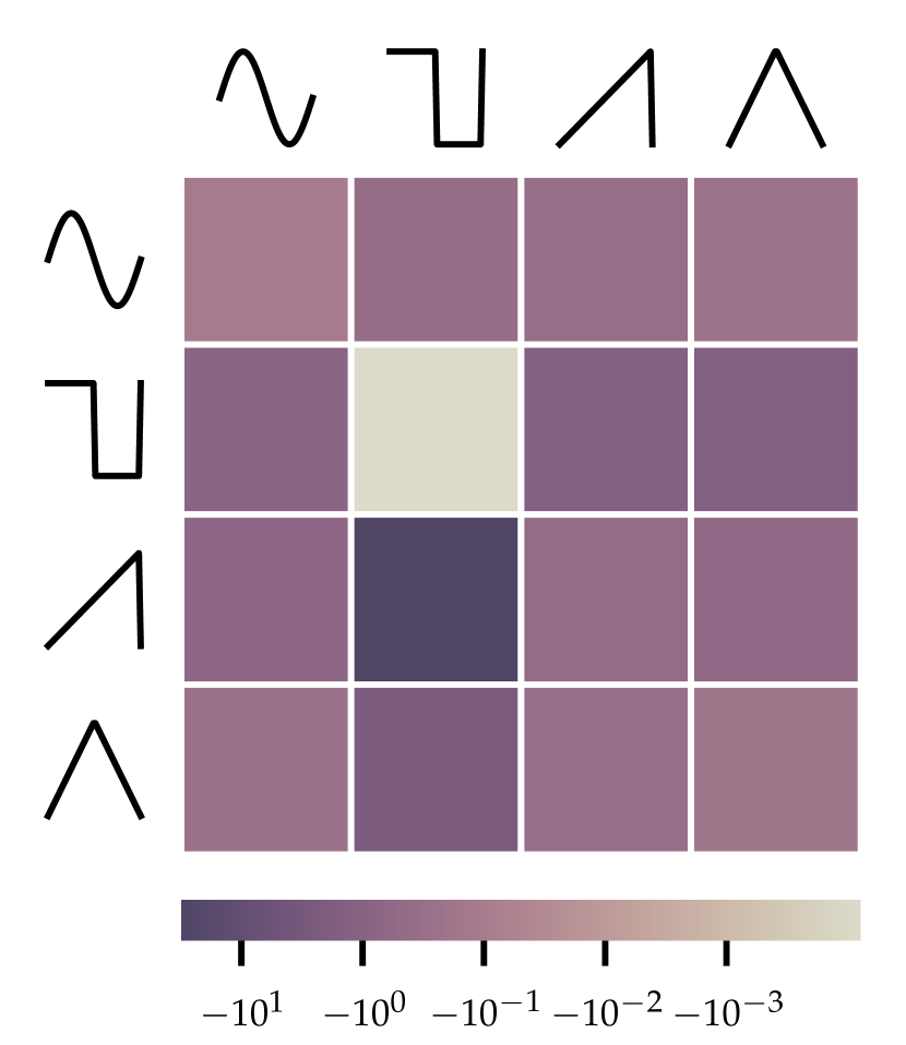
(c) $\sigma=0.027$

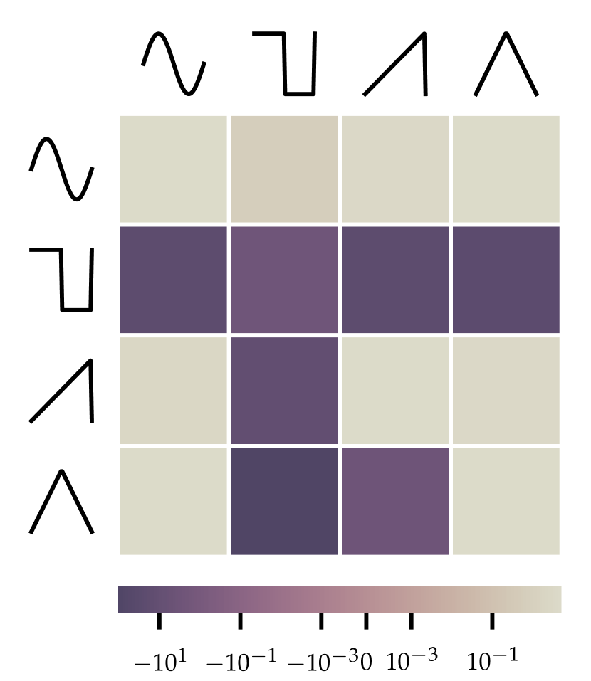
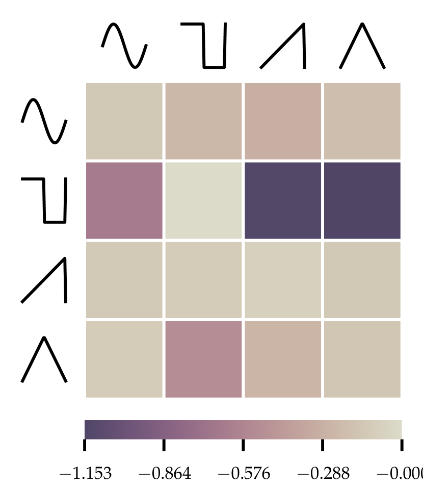
(d) $\sigma=0.077$

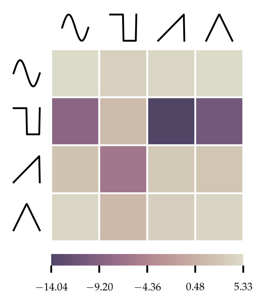
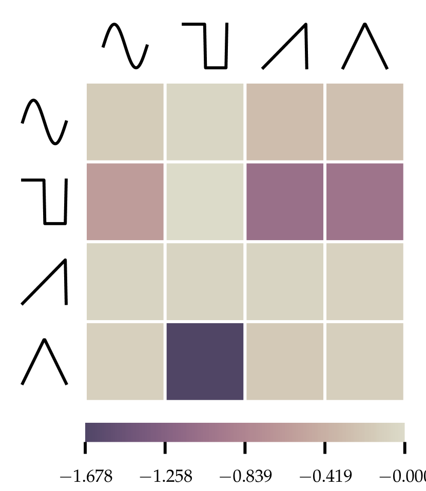
(e) $\sigma=0.129$

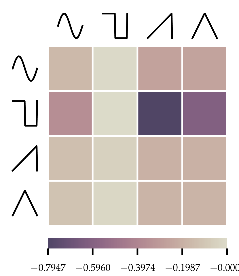
(f) $\sigma=0.359$

Figure 4: The cross-likelihood of the toy source channels under each model after conditioning the distribution on different levels of noise. The data noise level is going down and the conditional is going to the left. At the top is the FloWaveNet model and at the bottom of the WaveNet model.

3.4 Random and constant inputs

		sine	square	saw	triangle
input	$\sigma$
0.0	0.0	4.8e+00	-7.0e+02	4.4e+00	1.8e+00
	0.359	-5.0e-01	-3.1e+00	5.1e+00	-2.0e+11
$\mathcal{N}$(0, 0.5)	0.0	-2.7e+13	-3.4e+09	-1.4e+05	-1.1e+11
	0.359	4.4e+00	-5.8e+01	5.1e+00	-3.8e+05

Table 1: FloWaveNet: The mean log likelihood of a full receptive field of constant inputs $\{0,1\}$ for the noise-free and the widest noise-conditioned model.

Previous works [17][20][8] have pointed out that generative models tend to assign high likelihood values to constant inputs. We find the same holds true for generative priors trained on the Toy data dataset. Table 1 shows that for the noise-free model a constant zero input is highly likely, except under the square wave prior, which we assume stems from the square wave never having the value 0.0. When fine-tuning the model with a noise-conditioning of $\sigma=0.359$ the constant zero input becomes less likely for the sources sine and triangle but more likely for saw and square. To test whether the noise-conditioning results in simple constant inputs being unlikely but pure noise input in return becoming likely we evaluate the likelihood of noise drawn from a zero-centered Gaussian with reasonable wide variance for both the noise-free and noise-conditional model.

In Table 1, we see that for the noise-free prior model, a high variance input noise sampled from $\mathcal{N}(0,0.5)$ is highly unlikely. Evaluating the same input noise under the wider noise-conditioned prior model the input becomes more likely. For the sine and saw waveform the noise input is even as likely as a normal in-class input.

We read these results to support the previous interpretation that even a small amount of noise fine-tuning can have severe effects on the estimated density. The noise-free prior models have sharp likelihood peaks around true data, in which even small amounts of added noise are highly unlikely. The noise-conditioning of the flow models flattens these peaks in so far that noise and out-of-distribution samples become highly likely, even at small levels of noise-conditioning.

4 Conclusion

In this work, we show that contemporary generative models for modeling of audio signals also exhibit strong problems with out-of-distribution data as similarly described in [8] for models of image data. Our experiments reinforce a suspicion that was also experimentally found in prior work on image data. Current deep generative models do not learn a density that is discriminative against out-of-distribution samples. We show that in our case the models lose their ability to detect out-of-distribution samples when trained with additive noise which is added to smooth the learned densities. Therefore our work further demonstrates to be cautious when applying current flow-based models to data outside close bounds of their training distribution.

5 Appendix

5.1 Source separation with SGLD

For better understanding of the source separation approach we had in mind using the generative models as prior we give the implementation in Algorithm 1.

1:for $t=1\dots T$ do

2:     for $k=1\dots N$ do

3:         $\epsilon_{t}\sim\mathcal{N}(0,\bm{1})$

4:         $\Delta\bm{s}_{k}^{t}\leftarrow\bm{s}^{t}+\eta\cdot\nabla\log{p(\bm{s}^{t})}+2\sqrt{\eta}\epsilon_{t}$

5:     end for

6:     for $k=1\dots N$ do

7:         $\bm{s}_{k}^{t+1}\leftarrow\Delta\bm{s}_{k}^{t}-\frac{\eta}{\sigma^{2}}\cdot[\bm{m}-\frac{1}{N}\sum^{N}_{i}\bm{s}_{i}^{t}]$

8:     end for

9:end for

Algorithm 1 The Langevin sampling procedure for source separation is fairly straight forward. For a fixed number of steps $T$ we sample we take a step into the direction of the gradient under the priors and the gradient of the mixing constraint while adding Gaussian noise $\epsilon_{t}$.

5.2 Model and training details

We construct the flow models closely following the architecture of FloWaveNet [5] which we show in Figure 5. It combines the affine coupling layer proposed in RealNVP [1] with the Activation Normalization proposed in Glow [7] but does not learn the channel mixing function as in Glow and apply the fixed checkerboard masking over the channel dimension.

The WaveNets are constructed as described in the original WaveNet work [14]. As in the original work the outputs of the model at each time-point are modeled with a multinomial distribution with a size of 256 and therefore uses a cross-entropy loss for optimization. The quantization of the wave data is done with standard $\mu$-law encoding.

The hyperparameters for all for model architectures are listed in Table 2.

The models are trained with the Adam optimizer [6]. As all models are fully convolutional the input size is in no way regimented by the architecture, only in so far that we are avoiding padding in the lower layers nevertheless we fix the size of all frames to $2^{14}=16384$. The initial learning rate is set to $1e-4$ and decreased with $\gamma=0.6$ in a fixed five-step decrease schedule. The toy model is trained with a batch size of 5 and the musdb18 model with a batch size of 2. We train the two unconditional flows and the WaveNets are trained for each 150.000 steps. The fine-tuning with the added noise is each trained until convergence which in practice was achieved in 20.000 to 40.000 steps.

Figure 5: The building blocks for the FloWaveNet model. The model consists of $n_{b}$ blocks (left). Each block consists of $n_{f}$ flows (middle). In each flow we apply activation normalization, followed by the affine coupling (right), after which the binary mask for the even/odd mapping is inverted. The affine coupling layer uses a WaveNet with the even set as the input to output scaling $\log s$ and translation $t$ with which the odd set is transformed. The squeeze operator, squeezes the time-dimension into the channel dimension doubling the number of channels.

	blocks	flows	layers	kernel size	width
WaveNet (toy)	3	-	10	3	256
WaveNet (musdb18)	3	-	10	3	256
FloWaveNet (toy)	4	6	10	3	32
FloWaveNet (musdb18)	8	6	10	3	48

Table 2: The hyperparameters for the FloWaveNet and WaveNet models. In case of the WaveNet blocks refers to the blocks as described in the original WaveNet architecture [14] while in the FloWaveNet the layers refer to the layers of the WaveNet in the coupling layers.

References

- Dinh et al. [2017] Laurent Dinh, Jascha Sohl-Dickstein, and Samy Bengio. Density estimation using Real NVP. arXiv:1605.08803 [cs, stat], February 2017. URL http://arxiv.org/abs/1605.08803. arXiv: 1605.08803.
- Hochreiter & Schmidhuber [1997] Sepp Hochreiter and Jürgen Schmidhuber. Long Short-Term Memory. Neural Computation, 9(8):1735–1780, November 1997. ISSN 0899-7667. doi: 10.1162/neco.1997.9.8.1735. URL https://www.mitpressjournals.org/doi/10.1162/neco.1997.9.8.1735.
- Jayaram & Thickstun [2020] Vivek Jayaram and John Thickstun. Source Separation with Deep Generative Priors. arXiv:2002.07942 [cs, stat], February 2020. URL http://arxiv.org/abs/2002.07942. arXiv: 2002.07942.
- Kaspersen [2019] Esbern Torgard Kaspersen. HydraNet: A Network For Singing Voice Separation. 2019.
- Kim et al. [2019] Sungwon Kim, Sang-gil Lee, Jongyoon Song, Jaehyeon Kim, and Sungroh Yoon. FloWaveNet : A Generative Flow for Raw Audio. arXiv:1811.02155 [cs, eess], May 2019. URL http://arxiv.org/abs/1811.02155. arXiv: 1811.02155.
- Kingma & Ba [2017] Diederik P. Kingma and Jimmy Ba. Adam: A Method for Stochastic Optimization. arXiv:1412.6980 [cs], January 2017. URL http://arxiv.org/abs/1412.6980. arXiv: 1412.6980.
- Kingma & Dhariwal [2018] Diederik P. Kingma and Prafulla Dhariwal. Glow: Generative Flow with Invertible 1x1 Convolutions. arXiv:1807.03039 [cs, stat], July 2018. URL http://arxiv.org/abs/1807.03039. arXiv: 1807.03039.
- Nalisnick et al. [2019] Eric Nalisnick, Akihiro Matsukawa, Yee Whye Teh, Dilan Gorur, and Balaji Lakshminarayanan. Do Deep Generative Models Know What They Don’t Know? arXiv:1810.09136 [cs, stat], February 2019. URL http://arxiv.org/abs/1810.09136. arXiv: 1810.09136.
- Narayanaswamy et al. [2020] Vivek Narayanaswamy, Jayaraman J. Thiagarajan, Rushil Anirudh, and Andreas Spanias. Unsupervised Audio Source Separation using Generative Priors. arXiv:2005.13769 [cs, eess, stat], May 2020. URL http://arxiv.org/abs/2005.13769. arXiv: 2005.13769.
- Narayanaswamy et al. [2019] Vivek Sivaraman Narayanaswamy, Sameeksha Katoch, Jayaraman J. Thiagarajan, Huan Song, and Andreas Spanias. Audio Source Separation via Multi-Scale Learning with Dilated Dense U-Nets. arXiv:1904.04161 [cs, eess, stat], April 2019. URL http://arxiv.org/abs/1904.04161. arXiv: 1904.04161.
- Neal [2012] Radford M. Neal. MCMC using Hamiltonian dynamics. arXiv:1206.1901 [physics, stat], June 2012. URL http://arxiv.org/abs/1206.1901. arXiv: 1206.1901.
- Paszke et al. [2019] Adam Paszke, Sam Gross, Francisco Massa, Adam Lerer, James Bradbury, Gregory Chanan, Trevor Killeen, Zeming Lin, Natalia Gimelshein, Luca Antiga, Alban Desmaison, Andreas Kopf, Edward Yang, Zachary DeVito, Martin Raison, Alykhan Tejani, Sasank Chilamkurthy, Benoit Steiner, Lu Fang, Junjie Bai, and Soumith Chintala. PyTorch: An Imperative Style, High-Performance Deep Learning Library. In H. Wallach, H. Larochelle, A. Beygelzimer, F. d\textquotesingle Alché-Buc, E. Fox, and R. Garnett (eds.), Advances in Neural Information Processing Systems 32, pp. 8026–8037. Curran Associates, Inc., 2019. URL http://papers.nips.cc/paper/9015-pytorch-an-imperative-style-high-performance-deep-learning-library.pdf.
- Rafii et al. [2017] Zafar Rafii, Antoine Liutkus, Fabian-Robert Stöter, Stylianos Ioannis Mimilakis, and Rachel Bittner. MUSDB18 - a corpus for music separation, December 2017. URL https://zenodo.org/record/1117372. Version Number: 1.0.0 type: dataset.
- Rethage et al. [2018] Dario Rethage, Jordi Pons, and Xavier Serra. A Wavenet for Speech Denoising. arXiv:1706.07162 [cs], January 2018. URL http://arxiv.org/abs/1706.07162. arXiv: 1706.07162.
- Rezende & Mohamed [2016] Danilo Jimenez Rezende and Shakir Mohamed. Variational Inference with Normalizing Flows. arXiv:1505.05770 [cs, stat], June 2016. URL http://arxiv.org/abs/1505.05770. arXiv: 1505.05770.
- Stöter et al. [2018] Fabian-Robert Stöter, Antoine Liutkus, and Nobutaka Ito. The 2018 Signal Separation Evaluation Campaign. arXiv:1804.06267 [cs, eess], July 2018. URL http://arxiv.org/abs/1804.06267. arXiv: 1804.06267.
- Sønderby et al. [2017] Casper Kaae Sønderby, Jose Caballero, Lucas Theis, Wenzhe Shi, and Ferenc Huszár. Amortised MAP Inference for Image Super-resolution. arXiv:1610.04490 [cs, stat], February 2017. URL http://arxiv.org/abs/1610.04490. arXiv: 1610.04490.
- van den Oord et al. [2016a] Aäron van den Oord, Sander Dieleman, Heiga Zen, Karen Simonyan, Oriol Vinyals, Alex Graves, Nal Kalchbrenner, Andrew Senior, and Koray Kavukcuoglu. WaveNet: A Generative Model for Raw Audio. arXiv:1609.03499 [cs], September 2016a. URL http://arxiv.org/abs/1609.03499. arXiv: 1609.03499.
- van den Oord et al. [2016b] Aäron van den Oord, Nal Kalchbrenner, Oriol Vinyals, Lasse Espeholt, Alex Graves, and Koray Kavukcuoglu. Conditional Image Generation with PixelCNN Decoders. arXiv:1606.05328 [cs], June 2016b. URL http://arxiv.org/abs/1606.05328. arXiv: 1606.05328.
- van den Oord et al. [2017] Aäron van den Oord, Yazhe Li, Igor Babuschkin, Karen Simonyan, Oriol Vinyals, Koray Kavukcuoglu, George van den Driessche, Edward Lockhart, Luis C. Cobo, Florian Stimberg, Norman Casagrande, Dominik Grewe, Seb Noury, Sander Dieleman, Erich Elsen, Nal Kalchbrenner, Heiga Zen, Alex Graves, Helen King, Tom Walters, Dan Belov, and Demis Hassabis. Parallel WaveNet: Fast High-Fidelity Speech Synthesis. arXiv:1711.10433 [cs], November 2017. URL http://arxiv.org/abs/1711.10433. arXiv: 1711.10433.
- Welling & Teh [2011] Max Welling and Yee Whye Teh. Bayesian learning via stochastic gradient langevin dynamics. In Proceedings of the 28th International Conference on International Conference on Machine Learning, ICML’11, pp. 681–688, Bellevue, Washington, USA, June 2011. Omnipress. ISBN 978-1-4503-0619-5.
- Yosinski et al. [2014] Jason Yosinski, Jeff Clune, Yoshua Bengio, and Hod Lipson. How transferable are features in deep neural networks? arXiv:1411.1792 [cs], November 2014. URL http://arxiv.org/abs/1411.1792. arXiv: 1411.1792.
- Yu & Koltun [2016] Fisher Yu and Vladlen Koltun. Multi-Scale Context Aggregation by Dilated Convolutions. arXiv:1511.07122 [cs], April 2016. URL http://arxiv.org/abs/1511.07122. arXiv: 1511.07122.