The interaction of domain walls with fermions in the early Universe
Abstract
We consider the scalar field solitons and their interaction with the fermions in the early Universe. The analytical form of the reflection coefficient is obtained. The fermion mass is a function of the distance between the fermion and the soliton (wall). The function was approximated by the Woods-Saxon potential.
Keywords: domain wall, Dirac equation, PBH, early Universe
1 Introduction
Primordial black holes (PBHs) have been a source of significant interest for over 50 years. The possibility of the existence of such objects was predicted by Zeldovich and Novikov [1]. Despite the absence of direct evidence of their existence, there is a lot of observational data that can be interpreted in the framework of the hypothesis of the origin of black holes (BH) at the initial stages of the origin of the Universe [2, 3, 4].
In this paper, we base on the model of PBH formation as a result of the collapse of domain walls [5, 6, 7]. As a result of phase transitions during and after the inflationary stage, closed domain walls are formed. The formed non-spherical wall evolves: when interacting with hot plasma, the kinetic energy of the wall dissipates. As a result, the oscillations of the domain wall decay, the energy is transferred to the surrounding plasma, which leads to its additional heating. Further, the wall spheres and collapses into BH.
The rate of energy transfer from the domain wall to the surrounding plasma depends on the wall thickness, the initial plasma temperature and its density. The wall thickness is characterized by the parameters of the initial Lagrangian and can vary over a wide range. Plasma temperature and density depend on the moment the walls appear. Moreover, the dynamics of plasma parameters depends on whether it participates in cosmological expansion or is separated from it due to the gravitational well created by closed walls.
In this paper, we consider the fermion interaction with the scalar field solitons (walls).
2 Model of domain wall
Consider the domain wall model. We describe We describe the wall by a complex scalar field with a Lagrangian:
| (1) |
where - complex scalar field and is its phase. At the end of inflation, the field is captured by the potential minimum for which . Then we write the complex field in the form:
| (2) |
Substitution of the expression (2) into Lagrangian (1) gives Lagrangian, that describing the phase of complex scalar field:
| (3) |
The the phase is determined as follows [8]:
| (4) |
where we introduced the wall thickness parameter
| (5) |
The interaction of the fermions with the domain wall is
| (7) |
Then Lagrangian of fermions can be rewritten as
| (8) |
where - fermion mass.
3 Dirac equation
A description of the interaction between fermions and domain wall within the framework of the approach to solving the equation of motion is given in the papers [9, 10, 11] The result for the interaction of the wall with scalar particles is given in the monograph [12]. In the papers [9, 10, 11] the description of the domain wall is given by the kink solution: . In such model, the asymptotic fermion mass takes different values: . This problem does not arise for the Lagrangian (8): the fermion mass is the same on both sides of the wall.
The Dirac equation
| (9) |
holds for fermion Lagrangian (8) where function
| (10) |
is effective mass, depending on the coordinate in the coordinate perpendicular to the wall. Hereinafter, in asymptotics, we have: .
The fermion wave function is as follows
| (11) |
Here we put for simplicity, i.e. the component of the momentum in the plane of the domain wall is zero and the incident wave is perpendicular to the wall. Then the equation takes the form:
| (12) |
Hereafter, we choose the following representation of gamma matrices:
| (13) |
As a result of substitution, we obtain a system of equations for the bispinor components:
| (14) | |||
We obtain a similar system for the components if we replace: .
Let’s consider the following linear combinations of bispinor components:
| (15) | |||
As a result of such substitution we obtain a system:
| (16) | |||
Excluding the variables, we obtain the equations for the components :
| (17) |
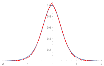
Let us carry out an approximation by a function for which the solution can be obtained in an analytical form. Let us choose the Woods-Saxon potential. The scattering problem for the Woods-Saxon potential is considered in detail in the papers [13, 14]: After approximation, the function takes the form
| (18) |
where parameters: , .
We solve the equation for two regions: and
Consider the region . We will solve the equation for (the superscript L denotes the region ). Let’s make a replacement:
| (19) |
Then the equation (17) takes the form:
| (20) |
Let’s consider the limit . Then, for the function we obtain superposition of two waves: incident and reflected waves:
| (23) |
The coefficients are determined by the formulas:
| (24) | |||
where . The asymptotic for is obtained by substituting solution (23) into the first equation of system (16). As a result, we obtain:
| (25) |
The region can be considered in the similar manner to obtain the function to the right of the wall.
In order to find coupling between coefficients and we match the solutions at :
| (26) | ||||
The normal component of the fermion current density is written as:
| (27) | ||||
Substitute the obtained functions As a result, we obtain The final form of the current
| (28) |
is obtained by substitution of the explicit form of functions and into the expressions for the current density. Here is the current density of the incident particles, - of the reflected ones.
The reflection and transmission coefficients are determined through the ratio of the current densities as follows
| (29) |
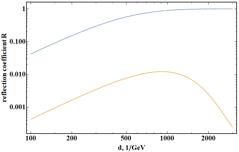
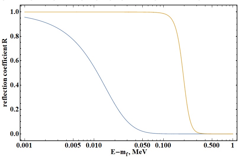
The coefficients are determined by the formulas (24). The results of calculating the reflection coefficient for electrons () are shown in Figure 3,3.
4 Conclusion
The deceleration of the primordial walls due to the interaction with the surrounding media is the important process that could influence the formation of the black holes clusters. In this paper, we have found the reflection probability of the fermions. This is necessary step for studying the cluster heating by the wall fluctuation.
Acknowledgements
This research was funded by the Ministry of Science and Higher Education of the Russian Federation, Project “Fundamental properties of elementary particles and cosmology” N 0723-2020-0041 and RFBR grant 19-02-00930. The work of S.R. is performed according to the Russian Government Program of Competitive Growth of Kazan Federal University.
References
- [1] Ya B Zel’dovich and ID Novikov “The hypothesis of cores retarded during expansion and the hot cosmological model” In Soviet Astronomy 10, 1967, pp. 602
- [2] Sebastien Clesse and Juan García-Bellido “Seven Hints for Primordial Black Hole Dark Matter” In Phys. Dark Univ. 22, 2018, pp. 137–146 DOI: 10.1016/j.dark.2018.08.004
- [3] A. Kashlinsky “Electromagnetic probes of primordial black holes as dark matter”, 2019 arXiv:1903.04424 [astro-ph.CO]
- [4] Bernard Carr and Florian Kuhnel “Primordial Black Holes as Dark Matter: Recent Developments”, 2020 arXiv:2006.02838 [astro-ph.CO]
- [5] Sergei G. Rubin, Alexander S. Sakharov and Maxim Yu. Khlopov “The Formation of primary galactic nuclei during phase transitions in the early universe” In J. Exp. Theor. Phys. 91, 2001, pp. 921–929 DOI: 10.1134/1.1385631
- [6] Konstantin M. Belotsky et al. “Clusters of primordial black holes” In Eur. Phys. J. C 79.3, 2019, pp. 246 DOI: 10.1140/epjc/s10052-019-6741-4
- [7] Heling Deng, Alexander Vilenkin and Masaki Yamada “CMB spectral distortions from black holes formed by vacuum bubbles” In JCAP 07, 2018, pp. 059 DOI: 10.1088/1475-7516/2018/07/059
- [8] R. Rajaraman “SOLITONS AND INSTANTONS. AN INTRODUCTION TO SOLITONS AND INSTANTONS IN QUANTUM FIELD THEORY”, 1982
- [9] Alejandro Ayala, Jamal Jalilian-Marian, Larry D. McLerran and Axel P. Vischer “Scattering in the presence of electroweak phase transition bubble walls” In Phys. Rev. D 49, 1994, pp. 5559–5570 DOI: 10.1103/PhysRevD.49.5559
- [10] D.. Steer and T. Vachaspati “Domain walls and fermion scattering in grand unified models” In Phys. Rev. D 73 American Physical Society, 2006, pp. 105021 DOI: 10.1103/PhysRevD.73.105021
- [11] Glennys R. Farrar and Jr. McIntosh “Scattering from a domain wall in a spontaneously broken gauge theory” In Phys. Rev. D 51, 1995, pp. 5889–5904 DOI: 10.1103/PhysRevD.51.5889
- [12] A. Vilenkin and E.P.. Shellard “Cosmic Strings and Other Topological Defects” Cambridge University Press, 2000
- [13] Piers Kennedy “The Woods-Saxon potential in the Dirac equation” In J. Phys. A 35, 2002, pp. 689–698 DOI: 10.1088/0305-4470/35/3/314
- [14] O. Panella, S. Biondini and A. Arda “New exact solution of the one dimensional Dirac Equation for the Woods-Saxon potential within the effective mass case” In J. Phys. A 43, 2010, pp. 325302 DOI: 10.1088/1751-8113/43/32/325302