Edge Universality for Nonintersecting Brownian Bridges

Abstract

In this paper we study fluctuations of extreme particles of nonintersecting Brownian bridges starting from $a_{1}\leqslant a_{2}\leqslant\cdots\leqslant a_{n}$ at time $t=0$ and ending at $b_{1}\leqslant b_{2}\leqslant\cdots\leqslant b_{n}$ at time $t=1$, where $\mu_{A_{n}}=(1/n)\sum_{i}\delta_{a_{i}},\mu_{B_{n}}=(1/n)\sum_{i}\delta_{b_{i}}$ are discretization of probability measures $\mu_{A},\mu_{B}$. Under regularity assumptions of $\mu_{A},\mu_{B}$, we show as the number of particles $n$ goes to infinity, fluctuations of extreme particles at any time $0<t<1$, after proper rescaling, are asymptotically universal, converging to the Airy point process.

New York University
E-mail: jh4427@nyu.edu

1 Introduction

One-dimensional Markov processes conditioned not to intersect form an important class of models which arise in the study of random matrix theory, growth processes, directed polymers and random tiling (dimer) models [27, 26, 49, 34, 53]. Among them, nonintersecting Brownian bridges, from conditioning $n$ standard Brownian bridges not to intersect, have been most studied. Their scaling limits give rise to determinantal point processes, which are believed to be universal objects for large families of interacting particle systems.

In the particular case, when nonintersecting Brownian bridges start at general position and end at the same position, say the origin, after a space-time transformation (1.4), it is the distribution of Dyson’s Brownian motion [23] on the real line. The positions of the particles at any time slice have the same distribution as the eigenvalues of the Gaussian unitary ensemble with external source [36]. In this case, as the number of particles goes to infinity, under proper scaling, the local statistics of nonintersecting Brownian bridges are universal, i.e. governed by the sine kernel inside the limit shape (in the bulk) [36, 39, 40, 7, 12], by the Airy kernel at the edge of the limit shape [51, 41, 7, 12], and by the Pearcey kernel at the cusp [5, 13, 15, 14, 52]. These kernels are universal since they appear in many other problems. In particular, the Airy process appears ubiquitously in the Kardar–Parisi–Zhang (KPZ) universality class [16], an important class of interacting particle systems and random growth models. The analysis of nonintersecting Brownian bridges greatly improves the understanding of the Airy process and the KPZ universality class, see [17, 19].

In this paper, we study the edge scaling limit of nonintersecting Brownian bridges with general boundary condition. They consist of $n$ standard Brownian bridges $\{(x_{1}(t),x_{2}(t),\cdots,x_{n}(t))\}_{0\leqslant t\leqslant 1}$ starting from $a_{1}\leqslant a_{2}\leqslant\cdots\leqslant a_{n}$ at time $t=0$ and ending at $b_{1}\leqslant b_{2}\leqslant\cdots\leqslant b_{n}$ at time $t=1$, conditioned not to intersect during the time interval $0<t<1$, i.e. $x_{i}(0)=a_{i},x_{i}(1)=b_{i}$ for $1\leqslant i\leqslant n$ and $x_{1}(t)<x_{2}(t)<\cdots<x_{n}(t)$ for $0<t<1$. We parametrize the starting and ending configurations as measures,

$$\mu_{A_{n}}=\frac{1}{n}\sum^{n}_{i=1}\delta_{a_{i}},\quad\mu_{B_{n}}=\frac{1}{n}\sum^{n}_{i=1}\delta_{b_{i}}.$$ (1.1)

If the measures $\mu_{A_{n}}$ and $\mu_{B_{n}}$ converge weakly to $\mu_{A}$ and $\mu_{B}$ respectively, as the number of particles $n$ goes to infinity, under mild assumptions of $\mu_{A},\mu_{B}$, it follows from [29, 30] that the empirical particle density of nonintersecting Brownian bridges with boundary data $\mu_{A_{n}},\mu_{B_{n}}$, converges

$$\frac{1}{n}\sum_{i=1}^{n}\delta_{x_{i}(t)}\rightarrow\rho_{t}^{*}(x){\rm d}x,\quad 0\leqslant t\leqslant 1,$$

in the weak sense. The measure valued process $\{\rho_{t}^{*}(x)\}_{0\leqslant t\leqslant 1}$ is given explicitly by a variational problem:

$$\{(\rho_{t}^{*},u_{t}^{*})\}_{0\leqslant t\leqslant 1}=\arg\inf\frac{1}{2}\left(\int_{0}^{1}\int_{\mathbb{R}}\left(u_{t}^{2}\rho_{t}+\frac{\pi^{2}}{3}\rho_{t}^{3}\right){\rm d}x{\rm d}t+\Sigma(\mu_{A})+\Sigma(\mu_{B})\right),$$ (1.2)

the $\inf$ is taken over all the pairs $\{(\rho_{t},u_{t})\}_{0\leqslant t\leqslant 1}$ such that $\partial_{t}\rho_{t}+\partial_{x}(\rho_{t}u_{t})=0$ in the sense of distributions, $\{\rho_{t}(\cdot)\}_{0\leqslant t\leqslant 1}\in{\mathcal{C}}([0,1],{\mathcal{M}}({\mathbb{R}}))$ and its initial and terminal data are given by

$$\lim_{t\rightarrow 0+}\rho_{t}(x){\rm d}x={\rm d}\mu_{A},\quad\lim_{t\rightarrow 1-}\rho_{t}(x){\rm d}x={\rm d}\mu_{B},$$

where convergence holds in the weak sense. We will discuss more on the variational problem in Section 2. Let $\Omega=\{(x,t)\in{\mathbb{R}}\times(0,1),\rho_{t}^{*}(x)>0\}$ be the region where $\rho_{t}^{*}(x)$ is positive. As in Figure 1, it turns out that the nonintersecting Brownian bridge occupies $\Omega$. The boundary of the region $\Omega$ is piecewise analytic, with possibly some cusp points. Let $\{({\sf a}(t),t)\}_{0\leqslant t\leqslant 1}$ be the left boundary of $\Omega$. For any $0<t<1$, in the neighborhood of $x={\sf a}(t)$, $\rho_{t}^{*}(x)$ has square root behavior

$$\rho_{t}^{*}(x)=\frac{{\sf s}(t)\sqrt{[x-{\sf a}(t)]_{+}}}{\pi}+\operatorname{O}(|x-{\sf a}(t)|^{3/2}),$$ (1.3)

and similar statement holds for the right boundary of $\Omega$.

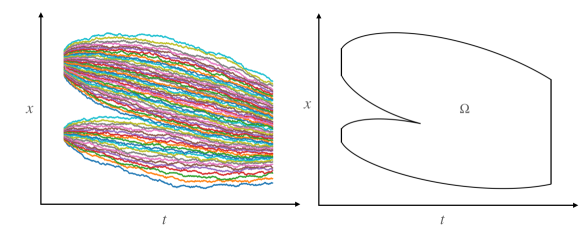
Figure 1: An example of nonintersecting Brownian bridges, and its support $\Omega$.

In this work, we study fluctuations of extreme particles of nonintersecting Brownian bridges. Under regularity assumptions of $\mu_{A},\mu_{B}$, we show as the number of particles $n$ goes to infinity, fluctuations of extreme particles at any time $0<t<1$, after proper rescaling, converge to the Airy point process.

Theorem 1.1.

Given probability measures $\mu_{A},\mu_{B}$ satisfying regularity Assumptions 3.1 and 3.2, and $\mu_{A_{n}},\mu_{B_{n}}$ the discretization of $\mu_{A},\mu_{B}$ satisfying Assumptions 3.3 and 3.4. Fix small ${\mathfrak{t}}>0$. For nonintersecting Brownian bridges with boundary data given by $\mu_{A_{n}},\mu_{B_{n}}$, as $n$ goes to infinity, fluctuations of extreme particles at time ${\mathfrak{t}}\leqslant t\leqslant 1-{\mathfrak{t}}$, after proper rescaling, converge to the Airy point process,

$$({\sf s}(t)n)^{2/3}(x_{1}(t)-{\sf a}(t),x_{2}(t)-{\sf a}(t),x_{3}(t)-{\sf a}(t),\cdots)\rightarrow\text{Airy Point Process}$$

The same statement holds for particles close to the right edge.

In Theorem 1.1, we need $\mu_{A_{n}}$ and $\mu_{B_{n}}$ to be sufficiently close to their limits $\mu_{A}$ and $\mu_{B}$. Especially, we do not allow outliers. Nonintersecting Brownian bridges with all but finitely many leaving from and returning to $0$, have been studied in [3, 2]. In this setting, the edge scaling limit is a new Airy process with wanderers, governed by an Airy-type kernel, with a rational perturbation.

A Brownian bridge $W(t)$ on $[0,1]$ from $a$ to $b$ i.e. $W(0)=a$ and $W(1)=b$ can be represented by a standard Brownian motion $B(t)$ starting from $a$ with drift $b$

$$W(t)=(1-t)B\left(\frac{t}{1-t}\right).$$ (1.4)

Under the transformation (1.4), nonintersecting Brownian bridges starting from $a_{1}\leqslant a_{2}\leqslant\cdots\leqslant a_{n}$ at time $t=0$ and ending at $b_{1}\leqslant b_{2}\leqslant\cdots\leqslant b_{n}$ at time $t=1$ become nonintersecting Brownian motions with drift [11, 50], i.e. $n$ standard Brownian motions starting from $a_{1}\leqslant a_{2}\leqslant\cdots\leqslant a_{n}$ at time $t=0$ and drifts $b_{1}\leqslant b_{2}\leqslant\cdots\leqslant b_{n}$ conditioned not to intersect. Our main result Theorem 1.1 implies the edge universality for nonintersecting Brownian motions with drift.

For nonintersecting Brownian bridges starting at time $t=0$ at $q$ and ending at time $t=1$ at $p$ prescribed positions, with $p,q\geqslant 2$, it was proven in [20] that the correlation functions of particle positions have a determinantal form, with a kernel expressed in terms of mixed multiple Hermite polynomials, which can be characterized by a Riemann-Hilbert problem of size $(p+q)\times(p+q)$. In the same setting, a partial differential equation for the probability to find all the particles in a given set has been obtained in [6]. However, it remains challenging to do an asymptotic analysis for those Rieman-Hilbert problems and partial differential equations. The only case where the asymptotic analysis was done is for $p=q=2$. In [18], the authors consider nonintersecting Brownian bridges, where $n/2$ particles go from $a$ to $b$, and $n/2$ particles go from $-a$ to $-b$. For a small separation of the starting and ending positions, they showed the kernels for the local statistics in the bulk and near the edges converge to the sine and Airy kernel in the large $n$ limit. For large separation of the starting and ending positions, those results have been extended in [20]. In the critical regime where the Brownian bridges fill two tangent ellipses in the time-space plane, a new correlation kernel, called the tacnode kernel, was obtained in [4, 21, 25, 35].

It seems to be a highly non-trivial problem to obtain concrete results about the scaling limit of nonintersecting Brownian bridges with general starting and ending configurations using its determinantal structure. In this paper we take a dynamical approach to study nonintersecting Brownian bridges. Let $\Delta_{n}$ be the Weyl chamber

$$\Delta_{n}=\{(z_{1},z_{2},\cdots,z_{n})\in{\mathbb{R}}^{n}:z_{1}<z_{2}<\cdots<z_{n}\}.$$ (1.5)

We reinterpret nonintersecting Brownian bridges as a random walk over $\Delta_{n}$ with drift. The transition probability density function of $n$ dimensional nonintersecting Brownian motions from ${\bm{x}}=(x_{1},x_{2},\cdots,x_{n})\in\Delta_{n}$ to ${\bm{y}}=(y_{1},y_{2},\cdots,y_{n})\in\Delta_{n}$ is given by the Karlin-McGregor formula [37]

$$p_{t}({\bm{x}},{\bm{y}})=\det\left[\sqrt{\frac{n}{2\pi t}}e^{-n(x_{i}-y_{j})^{2}/(2t)}\right]_{1\leqslant i,j\leqslant n}.$$ (1.6)

With the transition kernel (1.6), we can rewrite nonintersecting Brownian bridges as the following random walk over $\Delta_{n}$ with drift:

$${\rm d}x_{i}(t) =\frac{1}{\sqrt{n}}{\rm d}B_{i}(t)+\frac{1}{n}\partial_{x_{i}}\log p_{1-t}({\bm{x}}(t),{\bm{b}}){\rm d}t,\quad 1\leqslant i\leqslant n,$$ (1.7)

where ${\bm{x}}(t)=(x_{1}(t),x_{2}(t),\cdots,x_{n}(t))\in\Delta_{n}$, $\{B_{1}(t),B_{2}(t),\cdots,B_{n}(t)\}_{0\leqslant t\leqslant 1}$ are standard Brownian motions, and the drift $p_{1-t}({\bm{x}},{\bm{b}})$ is the heat kernel in the Weyl chamber,

$$-\partial_{t}p_{1-t}({\bm{x}},{\bm{b}})=\frac{1}{2n}\Delta p_{1-t}({\bm{x}},{\bm{b}}),\quad p_{1-t}({\bm{x}},{\bm{b}})=\det\left[\sqrt{\frac{n}{2\pi(1-t)}}e^{-n(x_{i}-b_{j})^{2}/(2(1-t))}\right]_{0\leqslant i,j\leqslant n}.$$ (1.8)

The limiting profile of nonintersecting Brownian bridges is characterized by the variational problem (1.2). We can use it to define a measure valued Hamiltonian system: given any probability measure $\mu\in{\mathcal{M}}({\mathbb{R}})$, and time $0\leqslant t\leqslant 1$ let

$$W_{t}(\mu)=-\frac{1}{2}\inf\left(\int_{t}^{1}\int_{\mathbb{R}}\rho_{s}\left(u_{s}^{2}+\frac{\pi^{2}}{3}\rho_{s}^{2}\right){\rm d}x{\rm d}s+\Sigma(\mu)+\Sigma(\mu_{B})\right),$$ (1.9)

where the non-commutative entropy $\Sigma(\mu)$ is defined in (2.3), the $\inf$ is taken over all the pairs $\{(\rho_{s},u_{s})\}_{t\leqslant s\leqslant{1}}$ such that $\partial_{s}\rho_{s}+\partial_{x}(\rho_{s}u_{s})=0$ in the sense of distributions, $\{\rho_{s}\}_{t\leqslant s\leqslant 1+\tau}\in{\mathcal{C}}([t,1],{\mathcal{M}}({\mathbb{R}}))$ and its initial and terminal data are given by

$$\lim_{s\rightarrow t+}\rho_{s}(x){\rm d}x=\mu,\quad\lim_{s\rightarrow 1-}\rho_{s}(x){\rm d}x=\mu_{B},$$

where convergence holds in the weak sense. Then the Hamilton’s principal function $W_{t}(\mu)$ satisfies the following Hamilton-Jacobi equation

$$\begin{split}-\partial_{t}W_{t}(\mu)&=\frac{1}{2}\int\left(\frac{\partial}{\partial x}\frac{\delta W_{t}}{\delta\mu}\right)^{2}{\rm d}\mu(x)+\int\frac{\partial}{\partial x}\frac{\delta W_{t}}{\delta\mu}H(\mu)(x){\rm d}\mu(x),\end{split}$$ (1.10)

where $H(\mu)(x)$ is the Hilbert transform of the measure $\mu$. There is a Riemann surface associated with the variational problem (1.9). Properties of $W_{t}(\mu)$ can be understood using tools for Riemann surfaces, i.e. Rauch variational formula and Hadamard’s Variation Formula.

Following Matytsin’s approach [42], we make an inverse Cole-Hopf transformation to convert the linear heat equation (1.8) to a nonlinear Hamilton-Jacobi equation, which is almost the same as (1.10) by taking $\mu=(1/n)\sum_{i}\delta_{x_{i}}$. Based on this observation, we make the following ansatz

$$\frac{1}{n}\frac{\partial}{\partial_{x_{k}}}\log\frac{p_{1-t}({\bm{x}},{\bm{b}})}{\prod_{i<j}(x_{i}-x_{j})}=\left.\frac{\partial}{\partial x}\frac{\delta W_{t}}{\delta\mu}\right|_{x=x_{k}}+{\mathcal{E}}^{(k)}_{t}({\bm{x}}),\quad 1\leqslant k\leqslant n.$$ (1.11)

Then we solve for the correction terms ${\mathcal{E}}^{(k)}_{t}({\bm{x}})$ by using Feynman-Kac formula. It turns out the correction terms ${\mathcal{E}}^{(k)}_{t}$ for $0\leqslant t\leqslant 1$ are of order $\operatorname{O}(1/n^{2})$. They have negligible influence on the random walk (1.7). By plugging the ansatz (1.11) into (1.7), and ignoring the correction terms ${\mathcal{E}}^{(k)}_{t}$, the system of stochastic differential equations becomes Dyson’s Brownian motion, with drifts depending on the particle configuration ${\bm{x}}(t)$. We analyze it using the method of characteristics, following the approach developed in [1, 32].

The heat kernel $p_{1-t}({\bm{x}},{\bm{b}})$ and the Hamilton’s principle function $W_{t}(\mu)$ are singular when $t$ approaches $1$, which makes the corresponding Hamilton-Jacobi equations hard to analyze. To overcome this problem, instead of studying nonintersecting Brownian bridges from ${\bm{a}}$ to ${\bm{b}}$ directly, we studied a weighted version of it. The weighted version corresponds to nonintersecting Brownian bridges with random boundary data at time $t=1$. There exists a natural choice of weight, such that at time $t=1$, the particle configuration of the weighted nonintersecting Brownian bridges concentrates around ${\bm{b}}$. We can analyze the weighted nonintersecting Brownian bridges using the above approach. Then by a coupling argument, we can transfer the edge universality result for the weighted nonintersecting Brownian bridges to the edge universality of nonintersecting Brownian bridges from ${\bm{a}}$ to ${\bm{b}}$.

We now outline the organization for the rest of the paper. In Section 2, we recall the variational problem which characterizes the limiting profile of nonintersecting Brownian bridges from [28]. In Section 3, We use the rate function of the variational problem to define a measure valued Hamiltonian system, and study its properties using tools from Riemann surfaces, i.e. Rauch variational formula and Hadamard’s Variation Formula. In Section 4, we define the weighted nonintersecting Brownian bridges, and reinterpret it as a drifted random walk. Based on the similarity to the Hamilton-Jacobi equation for the measure valued system, we make an ansatz for the drift term of the random walk. In Section 5, we solve for the correction term in the ansatz using Feynman-Kac formula. In Sections 6 we prove the optimal rigidity for the particle locations for this weighted nonintersecting Brownian bridges. And optimal rigidity estimates for nonintersecting Brownian bridges follow from a coupling argument in Section 7. Using optimal rigidity estimates as input in Section 8.1 we prove edge universality for nonintersecting Brownian bridges.

Notations

We denote ${\mathcal{M}}({\mathbb{R}})$ the set of probability measures over ${\mathbb{R}}$, and ${\mathcal{C}}([0,1],{\mathcal{M}}({\mathbb{R}}))$ the set of continuous measure valued process over $[0,1]$. We use ${\mathfrak{C}}$ to represent large universal constant, and ${\mathfrak{c}}$ a small universal constant, which may depend on other universal constants, i.e., the constants ${\mathfrak{a}},{\mathfrak{b}},{\mathfrak{t}}$ in Assumptions 3.2 and (3.3), and may be different from line by line. We write $a\vee b=\max\{a,b\}$ and $a\wedge b=\min\{a,b\}$. We write that $X=\operatorname{O}(Y)$ if there exists some universal constant such that $|X|\leqslant{\mathfrak{C}}Y$ . We write $X=\operatorname{o}(Y)$, or $X\ll Y$ if the ratio $|X|/Y\rightarrow\infty$ as $n$ goes to infinity. We write $X\asymp Y$ if there exist universal constants such that ${\mathfrak{c}}Y\leqslant|X|\leqslant{\mathfrak{C}}Y$. We say an event holds with overwhelming probability, if for any ${\mathfrak{C}}>0$, and $n\geqslant n_{0}({\mathfrak{C}})$ large enough, the event holds with probability at least $1-N^{-{\mathfrak{C}}}$.

Acknowledgements

The research of J.H. is supported by the Simons Foundation as a Junior Fellow at the Simons Society of Fellows.

2 Variational Principle

The transition probability density (1.6) of nonintersecting Brownian motions is closely related to the Harish-Chandra-Itzykson-Zuber integral formula [31, 33]. Let $A_{n},B_{n}$ be two $n\times n$ diagonal matrices, with diagonal entries given by $a_{1}\leqslant a_{2}\leqslant\cdots\leqslant a_{n}$ and $b_{1}\leqslant b_{2}\leqslant\cdots\leqslant b_{n}$ respectively, the Harish-Chandra-Itzykson-Zuber integral formula exactly computes the following integral

$$\begin{split}\int e^{n\operatorname{Tr}(A_{n}UB_{n}U^{*})}{\rm d}U=\frac{\prod_{j=1}^{n-1}j!}{n^{(n^{2}-n)/2}}\frac{\det[e^{na_{i}b_{j}}]_{i,j}}{\Delta(a_{1},a_{2},\cdots,a_{n})\Delta(b_{1},b_{2},\cdots,b_{n})},\end{split}$$ (2.1)

where $U$ follows the Haar probability measure of the unitary group and $\Delta$ denotes the Vandermonde determinant

$$\Delta(a_{1},a_{2},\cdots,a_{n})=\prod_{1\leqslant i<j\leqslant n}(a_{j}-a_{i}),\quad\Delta(b_{1},b_{2},\cdots,b_{n})=\prod_{1\leqslant i<j\leqslant n}(b_{j}-b_{i}).$$ (2.2)

We can rewrite the transition probability (1.6) of nonintersecting Brownian bridges by rescaling the Harish-Chandra-Itzykson-Zuber integral formula (2.1):

$$\begin{split}\frac{p_{1}({\bm{a}},{\bm{b}})}{\Delta({\bm{a}})\Delta({\bm{b}})}&=\frac{\det[\sqrt{n/2\pi}e^{-n(a_{i}-b_{j})^{2}/2}]_{i,j}}{\Delta(a_{1},a_{2},\cdots,a_{n})\Delta(b_{1},b_{2},\cdots,b_{N})}\\ &=\frac{{n}^{(n^{2}-n)/2}}{\prod_{j=1}^{n-1}j!}\prod_{i=1}^{n}\sqrt{n/2\pi}e^{-n(a_{i}^{2}+b_{i}^{2})/2}\int e^{n\operatorname{Tr}(A_{n}UB_{n}U^{*})}{\rm d}U.\end{split}$$

If the spectral measures $\mu_{A_{n}},\mu_{B_{n}}$ of $A_{n},B_{n}$ converge weakly towards $\mu_{A}$ and $\mu_{B}$ respectively, under mild assumptions, it was proven in [29, 30], see also [28, 22], that the Harish-Chandra-Itzykson-Zuber integral converges

$$\lim_{n\rightarrow\infty}\frac{1}{n^{2}}\log\int e^{n\operatorname{Tr}(A_{n}UB_{n}U^{*})}{\rm d}U=I(\mu_{A},\mu_{B}).$$

The asymptotics $I(\mu_{A},\mu_{B})$ of the Harish-Chandra-Itzykson-Zuber integral is characterized by a variational problem. We recall that for any probability measure $\mu\in{\mathcal{M}}({\mathbb{R}})$, we denote $\Sigma(\mu)$ the energy of its logarithmic potential, or its non-commutative entropy,

$$\Sigma(\mu)=\int\int\log|x-y|{\rm d}\mu(x){\rm d}\mu(y).$$ (2.3)

The following theorem is from [28, Theorem 2.1].

Theorem 2.1 ([28, Theorem 2.1]).

We assume that $\mu_{A},\mu_{B}$ are both compactly supported, then $I(\mu_{A},\mu_{B})$ is given by

$$I(\mu_{A},\mu_{B})=-\frac{1}{2}\inf\left(S(u,\rho)+\left(\Sigma(\mu_{A})+\Sigma(\mu_{B})\right)-\left(\int x^{2}{\rm d}\mu_{A}(x)+\int x^{2}{\rm d}\mu_{B}(x)\right)\right)+\text{const.}$$ (2.4)

where

$$S(u,\rho)=\int_{0}^{1}\int_{\mathbb{R}}\left(u_{t}^{2}\rho_{t}+\frac{\pi^{2}}{3}\rho_{t}^{3}\right){\rm d}x{\rm d}t,$$ (2.5)

the $\inf$ is taken over all the pairs $\{(\rho_{t},u_{t})\}_{0\leqslant t\leqslant 1}$ such that $\partial_{t}\rho_{t}+\partial_{x}(\rho_{t}u_{t})=0$ in the sense of distributions, $\{\rho_{t}(\cdot)\}_{0\leqslant t\leqslant 1}\in{\mathcal{C}}([0,1],{\mathcal{M}}({\mathbb{R}}))$ and its initial and terminal data are given by

$$\lim_{t\rightarrow 0+}\rho_{t}(x){\rm d}x={\rm d}\mu_{A},\quad\lim_{t\rightarrow 1-}\rho_{t}(x){\rm d}x={\rm d}\mu_{B},$$

where convergence holds in the weak sense.

The infimum in (2.4) is reached at a unique probability measure-valued path $\rho_{t}^{*}{\rm d}x\in{\mathcal{C}}([0,1],{\mathcal{M}}({\mathbb{R}}))$ such that for $t\in(0,1)$, $\rho_{t}^{*}{\rm d}x$ is absolutely continuous with respect to Lebesgue measure. The measure-valued path $\rho_{t}^{*}{\rm d}x\in{\mathcal{C}}([0,1],{\mathcal{M}}({\mathbb{R}}))$ describes the empirical particle locations of nonintersecting Brownian bridge (4.2): as $n$ goes to infinity

$$\left\{\frac{1}{n}\sum_{i=1}^{n}\delta_{x_{i}(t)}\right\}_{0\leqslant t\leqslant 1}\rightarrow\{\rho_{t}^{*}{\rm d}x\}_{0\leqslant t\leqslant 1}.$$

The minimizer $\{(\rho_{t}^{*}(\cdot),u^{*}_{t}(\cdot))\}_{0\leqslant t\leqslant 1}$ of the variational problem (2.4) can be described using the language of free probability, [28, Theorem 2.6].

Theorem 2.2 ([28, Theorem 2.6]).

There exist two non-commutative operators $\mathsf{a},\sf b$ with marginal distribution $(\mu_{A},\mu_{B})$ and a non-commutative brownian motion $\{\sf s_{t}\}_{0\leqslant t\leqslant 1}$ independent of $\sf a,\sf b$ in a non-commutative probability space $(\mathcal{A},\tau)$. The following free brownian bridge

$${\rm d}{\sf x}_{t}={\rm d}{\sf s}_{t}+\frac{{\sf b}-{\sf x}_{t}}{1-t}{\rm d}t,\quad{\sf x}_{0}=\sf a,\quad{\sf x}_{1}=\sf b,$$ (2.6)

at time $t$ has the law given by $\rho_{t}^{*}$, and

$$u_{t}^{*}=\frac{1}{t-1}\tau(\mathsf{x}_{t}-\mathsf{b}|\mathsf{x}_{t})+H(\rho^{*}_{t}),\qquad\rho_{t}^{*}(x){\rm d}x\quad a.s.$$ (2.7)

where $H(\rho_{t}^{*})$ is the Hilbert transform of $\rho_{t}^{*}$.

3 Complex Burger’s equation

We denote the minimizer of the variational problem (2.4) as $\{(\rho_{t}^{*}(\cdot),u^{*}_{t}(\cdot))\}_{0\leqslant t\leqslant 1}$ and let $\Omega$ be the domain where $\rho^{*}_{t}(x)>0$,

$$\Omega=\{(x,t)\in{\mathbb{R}}\times(0,1):\rho^{*}_{t}(x)>0\}.$$ (3.1)

Then it follows from [8, Lemma 7.2], $\Omega$ is a bounded simply connected (it does not contain holes) open domain in ${\mathbb{R}}\times[0,1]$. Moreover, the free brownian bridge representation, Theorem 2.2, implies that the infimum $\{(\rho_{t}^{*}(\cdot),u^{*}_{t}(\cdot))\}_{0\leqslant t\leqslant 1}$ is analytic in $\Omega$. In the rest of the paper, we call $\partial\Omega\cap{\mathbb{R}}\times(0,1)$ the left and right boundary of $\Omega$; $\partial\Omega\cap{\mathbb{R}}\times\{0\}$ the bottom boundary of $\Omega$; $\partial\Omega\cap{\mathbb{R}}\times\{1\}$ the top boundary of $\Omega$.

As derived in [28, Theorem 2.1], the Euler-lagurange equation for the variational problem (2.5) implies that the minimizer $\{(\rho_{t}^{*}(\cdot),u^{*}_{t}(\cdot))\}_{0\leqslant t\leqslant 1}$ satisfies

$$\partial_{t}u_{t}^{*}=-\frac{1}{2}\partial_{x}\left((u_{t}^{*})^{2}-\pi^{2}(\rho_{t}^{*})^{2}\right),\quad(x,t)\in\Omega.$$

If we define

$$f_{t}(x)=u^{*}_{t}(x)-\mathrm{i}\pi\rho^{*}_{t}(x),$$ (3.2)

then $f(x,t)$ satisfies the complex Burger’s equation

$$\partial_{t}f_{t}(x)+f_{t}(x)\partial_{x}f_{t}(x)=0,\quad(x,t)\in\Omega.$$ (3.3)

In physics literature, the complex Burger’s equation description of the Harish-Chandra-Itzykson-Zuber integral formula first appeared in the work of Matytsin [42]. Its rigorous mathematical study appears in the work of Guionnet [28].

The complex Burger’s equation can be solved using characteristic method. The argument in [38, Corollary 1] implies that there exists an analytic function of $Q$ of two variables such that the solution of (3.3) satisfies

$$Q(f_{t}(x),x-tf_{t}(x))=0,$$ (3.4)

where the analytic function $Q$ is determined by the boundary condition at $t=0,1$: $-\mathop{\mathrm{Im}}[f_{0}(x)]{\rm d}x/\pi={\rm d}\mu_{A}$ and $-\mathop{\mathrm{Im}}[f_{1}(x)]{\rm d}x/\pi={\rm d}\mu_{B}$. By the definition (3.1), on $\Omega$ we have $\mathop{\mathrm{Im}}[f_{t}(x)]<0$. We can recover $(x,t)$ from $(f_{t}(x),x-tf_{t}(x))$, by noticing that $t=-\mathop{\mathrm{Im}}[x-tf_{t}(x)]/\mathop{\mathrm{Im}}[f_{t}(x)]$. Thus, the map

$$\pi_{Q}:(x,t)\in\Omega\mapsto(f_{t}(x),x-tf_{t}(x))$$ (3.5)

is an orientation preserving diffeomorphism from $\Omega$ onto its image.

Thanks to the free Brownian bridge representation (2.6), $\rho_{t}^{*}$ is the law of

$$(1-t)\sf a+t\sf b+\sqrt{t(1-t)}\sf s,$$

where $\sf s$ is a free semi-circular law and it is free with $\sf a,\sf b$. As a direct consequence of [10], for any $t\in(0,1)$, and $x_{0}\in{\mathbb{R}}$ such that $(t,x_{0})\in\partial\Omega$, in a small neighborhood of $x_{0}$,

$$\rho_{t}^{*}(x)\leqslant\left({3\over 4\pi^{3}t^{2}(1-t)^{2}}\right)^{1\over 3}(x-x_{0})^{1\over 3},\quad x\in\operatorname{supp}\rho_{t}^{*}.$$

Especially, for $0<t<1$, $f_{t}(x)$ is continuous up to the boundary of $\Omega$. We can glue $f_{t}(x)$ and its complex conjugate along the left and right boundary of $\Omega$ (where $f_{t}(x)\in{\mathbb{R}}$). This map is orientation preserving and unramified by the discussion above, and so a covering map of $Q(f,z)=0$. Moreover, the Riemann surface $Q(f,z)=0$ is of the same genus as $\Omega$, which has genus zero [8, Lemma 7.2]. As a consequence the left and right boundary of the region $\Omega$ is piecewise analytic, with some cusp points. For any $0<t<1$, the density $\rho_{t}^{*}(x)$ is analytic. Moreover, $\rho_{t}^{*}(x)$ has square root behavior at left and right boundary points (which are not cusp points) of its support. Let $\{({\sf a}(t),t)\}_{0\leqslant t\leqslant 1}$ be the left boundary of $\Omega$. For any $0<t<1$, in the neighborhood of $x={\sf a}(t)$, $\rho_{t}^{*}(x)$ has square root behavior

$$\rho_{t}^{*}(x)=\frac{{\sf s}(t)\sqrt{[x-{\sf a}(t)]_{+}}}{\pi}+\operatorname{O}(|x-{\sf a}(t)|^{3/2}).$$ (3.6)

With the Riemann surface $Q(f,z)=0$, we can extend the function (3.2) $f_{t}(x)$ from $\{x:(x,t)\in\Omega\}$ to a meromorphic function on the Riemann surface $Q(f,z)=0$. At time $t$, the equation $\{(f,z)\in{\mathbb{C}}\times{\mathbb{C}}:Q(f,z-tf)=0\}$ defines a Riemann surface ${\mathcal{C}}_{t}$. We notice ${\mathcal{C}}_{0}$ is simply the Riemann surface $Q(f,z)=0$, and ${\mathcal{C}}_{t}$ can be obtained from ${\mathcal{C}}_{0}$ by the characteristic flow:

$$Z_{0}=(f,z)\in{\mathcal{C}}_{0}\mapsto Z_{t}=(f,z+tf)\in{\mathcal{C}}_{t}.$$ (3.7)

As a consequence, the family of Riemann surfaces $\{{\mathcal{C}}_{t}\}_{0\leqslant t\leqslant 1}$ are homeomorphic to each other. Comparing with (3.4), this gives a natural extension for $f_{t}(x)$ from $\{x:(x,t)\in\Omega\}$ to the Riemann surface ${\mathcal{C}}_{t}$. In this way $f_{t}:Z=(f,z)\in{\mathcal{C}}_{t}\mapsto f\in{\mathbb{C}}$. If the context is clear we will simply write $f_{t}(Z)=f_{t}((f,z))$ as $f_{t}(z)$ for $Z=(f,z)\in{\mathcal{C}}_{t}$. The complex Burger’s equation (3.3) extend naturally to $f_{t}$:

$$\partial_{t}f_{t}(Z)+\partial_{z}f_{t}(Z)f_{t}(Z)=0,\quad 0\leqslant t\leqslant 1,\quad Z\in{\mathcal{C}}_{t}.$$ (3.8)

3.1 Regularity Assumptions

In the rest of this paper, we will make the assumption that $\mu_{B}$ is regular enough, such that the solution of the complex Burger’s equation (3.3) can be extended to $t=1+\tau$ with some $\tau>0$.

Assumption 3.1 (Regularity).

The probability measures $\mu_{A},\mu_{B}$ are regular in the sense: There exists some constant $\tau>0$, the solution of the complex Burger’s equation (3.3), with boundary conditions:

$$-\frac{1}{\pi}\mathop{\mathrm{Im}}[f_{0}(x)]{\rm d}x={\rm d}\mu_{A},\quad-\frac{1}{\pi}\mathop{\mathrm{Im}}[f_{1}(x)]{\rm d}x={\rm d}\mu_{B},$$

can be extended up to time $t=1+\tau$.

Under Assumption 3.1, we denote the extension by $\{f_{t}(x)\}_{1\leqslant t\leqslant 1+\tau}$, and

$$-\frac{1}{\pi}\mathop{\mathrm{Im}}[f_{1+\tau}(x)]{\rm d}x={\rm d}\mu_{C}.$$

for some probability measure $\mu_{C}$.

For the following variational problem with boundary data $\mu_{A},\mu_{C}$,

$$-\frac{1}{2}\inf\left(\int_{0}^{1+\tau}\int_{\mathbb{R}}\rho_{t}\left(u_{t}^{2}+\frac{\pi^{2}}{3}\rho_{t}^{2}\right){\rm d}x{\rm d}t+\Sigma(\mu_{A})+\Sigma(\mu_{C})\right),$$ (3.9)

the $\inf$ is taken over all the pairs $\{(\rho_{t},u_{t})\}_{0\leqslant t\leqslant{1+\tau}}$ such that $\partial_{t}\rho_{t}+\partial_{x}(\rho_{t}u_{t})=0$ in the sense of distributions, $\{\rho_{t}\}_{0\leqslant t\leqslant 1+\tau}\in{\mathcal{C}}([0,1+\tau],{\mathcal{M}}({\mathbb{R}}))$ and its initial and terminal data are given by

$$\lim_{t\rightarrow 0+}\rho_{t}(x){\rm d}x={\rm d}\mu_{A},\quad\lim_{t\rightarrow(1+\tau)-}\rho_{t}(x){\rm d}x={\rm d}\mu_{C},$$

where convergence holds in the weak sense. The minimizer $\{(\rho_{t}^{*}(\cdot),u^{*}_{t}(\cdot))\}_{0\leqslant t\leqslant 1+\tau}$ of (3.9), satisfies

$$\rho_{B}(x){\rm d}x\mathrel{\mathop{:}}=\rho_{1}^{*}(x){\rm d}x={\rm d}\mu_{B},$$

and the density $\rho_{B}(x)$ is analytic. For our analysis, we need to assume that $\rho_{B}(x)$ has a connected support and is non-critical.

Assumption 3.2 (Non-critical).

We assume that $\mu_{B}$ has a connected support and is non-critical, that is, there exists a constant ${\mathfrak{b}}>0$ such that,

$$\rho_{B}(x)=S(x)\sqrt{(x-{\sf a}(1))({\sf b}(1)-x)},\quad S(x)\geqslant{\mathfrak{b}},\quad x\in[{\sf a}(1),{\sf b}(1)].$$

Under Assumptions 3.1 and 3.2, by shrinking $\tau$ if necessary, we can take ${\rm d}\mu_{C}=\rho_{C}(x){\rm d}x$ to be analytic, non-critical and have a connected support, i.e. $\rho_{C}$ also satisfies Assumption 3.2.

We make the following assumptions on the boundary data $\mu_{A_{n}},\mu_{B_{n}}$ of our nonintersecting Brownian bridges. We can take $\mu_{A_{n}},\mu_{B_{n}}$ to be the $1/n$-quantiles of measures $\mu_{A},\mu_{B}$. Assumptions 3.3 and 3.4 are slightly more general.

Assumption 3.3.

We assume the initial data $\mu_{A_{n}}$ of nonintersecting Brownian bridges satisfies: there exists a constant ${\mathfrak{a}}>0$ such that for any $\varepsilon>0$, and $n$ sufficiently large,

$$\left|\int\frac{{\rm d}\mu_{A}(x)-{\rm d}\mu_{A_{n}}(x)}{x-z}\right|\leqslant\frac{(\log n)^{\mathfrak{a}}}{n},$$ (3.10)

uniformly for any $\{z\in{\mathbb{C}}_{+}:\operatorname{dist}(z,\operatorname{supp}(\mu_{A}))\geqslant\varepsilon\}$.

Assumption 3.4.

We assume the terminal data $\mu_{B_{n}}$ of nonintersecting Brownian bridges satisfies: there exists a constant ${\mathfrak{a}}>0$ such

$$\gamma_{i-(\log n)^{\mathfrak{a}}}\leqslant b_{i}\leqslant\gamma_{i+(\log n)^{\mathfrak{a}}},\quad\frac{i+1/2}{n}=\int_{-\infty}^{\gamma_{i}}\rho_{B}(x){\rm d}x,\quad 1\leqslant i\leqslant n,$$ (3.11)

where we use the convention $\gamma_{i}=-\infty$ for $i\leqslant 0$ and $\gamma_{i}=+\infty$ for $i\geqslant n$, and

$$b_{1}\geqslant{\sf a}(1)-\frac{(\log n)^{{\mathfrak{a}}}}{n^{2/3}},\quad b_{n}\leqslant{\sf b}(1)+\frac{(\log n)^{{\mathfrak{a}}}}{n^{2/3}}.$$

Assumption 3.3 guaranteed that for any analytic test function $f(x)$, by a contour integral

$$\left|\int f(x)({\rm d}\mu_{A}(x)-{\rm d}\mu_{A_{n}}(x))\right|\lesssim\frac{(\log n)^{\mathfrak{a}}}{n}.$$ (3.12)

We will see in Section 6, the assumption is necessary for the optimal rigidity estimates. We remark that the assumption (3.11) implies (3.10) with possibly a different ${\mathfrak{a}}$. In this sense Assumption 3.4 is stranger than Assumption 3.3. Moreover, in Assumption 3.10 we allow to have outliers which are distance $\operatorname{o}(1)$ away from $\operatorname{supp}(\mu_{A})$. But, we do not allow outliers with are distance $\operatorname{O}(1)$ away from the support. Nonintersecting Brownian bridges with all but finitely many leaving from and returning to $0$, have been studied in [3, 2]. In this setting, the edge scaling limit is a new Airy process with wanderers, governed by an Airy-type kernel, with a rational perturbation.

The same as in (3.4), we can use the minimizer $\{(\rho_{t}^{*}(\cdot),u^{*}_{t}(\cdot))\}_{0\leqslant t\leqslant 1+\tau}$ of the variational problem (3.9), to construct the family of Riemann surfaces $\{{\mathcal{C}}_{t}\}_{0\leqslant t\leqslant 1+\tau}$, and extend $f_{t}(\cdot)$ to the Riemann surface ${\mathcal{C}}_{t}$ for $0\leqslant t\leqslant 1+\tau$. They satisfy the complex Burger’s equation

$$\partial_{t}f_{t}(Z)+\partial_{z}f_{t}(Z)f_{t}(Z)=0,\quad 0\leqslant t\leqslant 1+\tau,\quad Z\in{\mathcal{C}}_{t}.$$ (3.13)

The boundary conditions are $-\mathop{\mathrm{Im}}[f_{0}(x)]{\rm d}x/\pi={\rm d}\mu_{A}$ and $-\mathop{\mathrm{Im}}[f_{1+\tau}(x)]{\rm d}x/\pi={\rm d}\mu_{C}$.

Figure 2: We can identify the Riemann surface ${\mathcal{C}}_{0}$ with two copies of $\Omega$ gluing together. These curves $\{(f_{s}(x;\mu,t),x):(x,s)\in\Omega^{\mu,t}\}$ and $\{(\overline{f_{s}(x;\mu,t)},x):(x,s)\in\Omega^{\mu,t}\}$ cut the Riemann surface ${\mathcal{C}}_{s}^{\mu,t}$ into two parts: ${\mathcal{C}}_{s}^{\mu,t,-},{\mathcal{C}}_{s}^{\mu,t,+}$. ${\mathcal{C}}_{s}^{\mu,t,-}$ corresponds to $\{(x,r):(x,r)\in\Omega^{\mu,t},t\leqslant r\leqslant s\}$, and ${\mathcal{C}}_{s}^{\mu,t,+}$ corresponds to $\{(x,r):(x,r)\in\Omega,s\leqslant r\leqslant 1+\tau\}$.

We can reformulate our boundary conditions $-\mathop{\mathrm{Im}}[f_{0}(x)]{\rm d}x/\pi={\rm d}\mu_{A}$, $-\mathop{\mathrm{Im}}[f_{1+\tau}(x)]{\rm d}x/\pi={\rm d}\mu_{C}$ in terms of the residuals of the $1$-form $f_{0}(Z){\rm d}z$ over ${\mathcal{C}}_{0}$. Let $\Omega=\{(x,t)\in{\mathbb{R}}\times(0,1+\tau):\rho^{*}_{t}(x)>0\}$. We recall that using the map (3.5),

$$\pi_{Q}:(x,t)\in\Omega\mapsto(f_{t}(x),x-tf_{t}(x))\in{\mathcal{C}}_{0},$$ (3.14)

the Riemann surface ${\mathcal{C}}_{0}$ can be identified as gluing two copies of $\Omega$ along their left and right boundaries, and has cuts along the top and bottom boundaries of $\Omega$. The $1$-form $f_{0}(Z){\rm d}z$ has residuals along the bottom boundary of $\Omega$ corresponding to time $t=0$, and along the top boundary of $\Omega$ corresponding to time $t=1+\tau$, as in Figure 2. The boundary condition at time $t=0$, $-\mathop{\mathrm{Im}}[f_{0}(x)]{\rm d}x/\pi={\rm d}\mu_{A}$ gives that the residual of $f_{0}(Z){\rm d}z$ along the bottom boundary of $\Omega$ is given by

$$\frac{1}{\pi}\mathop{\mathrm{Im}}[f_{0}(x){\rm d}x]=-{\rm d}\mu_{A}(x).$$ (3.15)

For the boundary condition at time $t={1+\tau}$, $-\mathop{\mathrm{Im}}[f_{1+\tau}(x)]{\rm d}x/\pi={\rm d}\mu_{C}$, we use the characteristic flow (3.7), which send $Z_{0}=(f,z)\in{\mathcal{C}}_{0}$ to $Z_{1+\tau}=(f,z+(1+\tau)f)\in{\mathcal{C}}_{1+\tau}$

$$f_{1+\tau}(Z_{1+\tau})=f_{1+\tau}((f,z+(1+\tau)f))=f=f_{0}((f,z))=f_{0}(Z_{0}).$$

Let

$$f_{1+\tau}(x)=\gamma(x)-\mathrm{i}\pi\rho_{C}(x),\quad x\in\operatorname{supp}(\mu_{C}),$$

where $\gamma:\operatorname{supp}(\rho_{C})\mapsto{\mathbb{R}}$ is analytic. Then the preimage of $\{(f_{1+\tau}(x),x):x\in\operatorname{supp}(\rho_{C})\}$ under the characteristic flow consists of two curves in ${\mathcal{C}}_{0}$, which can be parametrized as

$$\left\{(f,z)=\left(\gamma(x)-\mathrm{i}\pi\rho_{C}(x),x+(1+\tau)(-\gamma(x)+\mathrm{i}\pi\rho_{C}(x))\right):x\in\operatorname{supp}(\rho_{C})\right\},$$ (3.16)

and its complex conjugate. Thus the residual of $f_{0}(Z){\rm d}z$ along the top boundary of $\pi_{Q}(\Omega)$ is given by

$$\frac{1}{\pi}\mathop{\mathrm{Im}}\left[(\gamma(x)-\mathrm{i}\pi\rho_{C}(x)){\rm d}(x+(1+\tau)(-\gamma(x)+\mathrm{i}\pi\rho_{C}(x)))\right]=-\rho_{C}(x){\rm d}x+(1+\tau){\rm d}\gamma(x)\rho_{C}(x).$$

Remark 3.5.

We remark that the residuals of $f_{0}(Z){\rm d}z$ along the bottom and top boundaries of $\Omega$, (3.15) and (3.16), uniquely determines the Riemann surface ${\mathcal{C}}_{0}:Q(f,z)=0$. However, it is not easy to directly write down the expression of $f$.

3.2 More General Boundary Condition

Slightly more general than (3.9), we can consider the following functional, for any probability measure $\mu$, and time $0\leqslant t\leqslant 1$,

$$W_{t}(\mu)=-\frac{1}{2}\inf\left(\int_{t}^{1+\tau}\int_{\mathbb{R}}\rho_{s}\left(u_{s}^{2}+\frac{\pi^{2}}{3}\rho_{s}^{2}\right){\rm d}x{\rm d}s+\Sigma(\mu)+\Sigma(\mu_{C})\right),$$ (3.17)

the $\inf$ is taken over all the pairs $\{(\rho_{s},u_{s})\}_{t\leqslant s\leqslant{1+\tau}}$ such that $\partial_{s}\rho_{s}+\partial_{x}(\rho_{s}u_{s})=0$ in the sense of distributions, $\{\rho_{s}\}_{t\leqslant s\leqslant 1+\tau}\in{\mathcal{C}}([t,1+\tau],{\mathcal{M}}({\mathbb{R}}))$ and its initial and terminal data are given by

$$\lim_{s\rightarrow t+}\rho_{s}(x){\rm d}x=\mu,\quad\lim_{s\rightarrow(1+\tau)-}\rho_{s}(x){\rm d}x=\mu_{C},$$

where convergence holds in the weak sense. Similarly to Theorem 2.2, (3.17) corresponds to certain free Brownian bridge $\{\sf x_{s}\}_{t\leqslant s\leqslant 1+\tau}$, with the law of $\sf x_{t}$ and $\sf x_{1+\tau}$ given by $\mu$ and $\mu_{C}$ respectively. The same as (3.3), if we denote the minimizer of (3.17) as $\{(\rho_{s}^{*}(\cdot;\mu,t),u_{s}^{*}(\cdot;\mu,t))\}_{t\leqslant s\leqslant 1}$ and

$$f_{s}(x;\mu,t)=u^{*}_{s}(x;\mu,t)-\mathrm{i}\pi\rho^{*}_{s}(x;\mu,t),\quad t\leqslant s\leqslant 1+\tau,$$ (3.18)

then $f_{s}(x;\mu,t)$ satisfies the complex Burger’s equation

$$\partial_{s}f_{s}(x;\mu,t)+f_{s}(x;\mu,t)\partial_{x}f_{s}(x;\mu,t)=0,\quad(x,s)\in\Omega^{\mu,t}\mathrel{\mathop{:}}=\{(x,s)\in{\mathbb{R}}\times(t,1+\tau):\rho_{s}^{*}(x;\mu,t)>0\}.$$ (3.19)

There exists an analytic function $Q^{\mu,t}$ of two variables such that the solution of (3.19) satisfies

$$Q^{\mu,t}(f_{s}(x;\mu,t),x-sf_{s}(x;\mu,t))=0,\quad t\leqslant s\leqslant 1+\tau.$$ (3.20)

With the analytic function $Q^{\mu,t}$, we can define the Riemann surface: ${\mathcal{C}}^{\mu,t}_{s}=\{(f,z)\in{\mathbb{C}}\times{\mathbb{C}}:Q^{\mu,t}(f,z-sf)=0\}$. Comparing with (3.20), this gives a natural extension for $f_{s}(x;\mu,t)$ from $\{x:(x,s)\in\Omega^{\mu,t}\}$ to the Riemann surface ${\mathcal{C}}_{s}^{\mu,t}$. In this way $f_{s}:Z=(f,z)\in{\mathcal{C}}_{s}^{\mu,t}\mapsto f\in{\mathbb{C}}$. The complex Burger’s equation extend naturally to $f_{s}$:

$$\partial_{s}f_{s}(Z;\mu,t)+\partial_{z}f_{s}(Z;\mu,t)f_{s}(Z;\mu,t)=0,\quad t\leqslant s\leqslant 1+\tau,\quad Z\in{\mathcal{C}}_{s}^{\mu,t}.$$ (3.21)

Similarly to (3.7), for $t\leqslant s\leqslant 1+\tau$, ${\mathcal{C}}^{\mu,t}_{s}$ can be obtained from ${\mathcal{C}}^{\mu,t}_{t}$ by the characteristic flow:

$$Z_{t}=(f,z)\in{\mathcal{C}}^{\mu,t}_{t}\mapsto Z_{s}=(f,z+(s-t)f)\in{\mathcal{C}}^{\mu,t}_{s}.$$ (3.22)

Using the map

$$\pi_{Q^{\mu,t}}:(x,r)\in\Omega^{\mu,t}\mapsto(f_{r}(x;\mu,t),x-(r-t)f_{r}(x;\mu,t))\in{\mathcal{C}}_{t}^{\mu,t},$$ (3.23)

we can identify ${\mathcal{C}}_{t}^{\mu,t}$ with two copies of $\Omega^{\mu,t}$ gluing along the left and right boundaries of $\Omega^{\mu,t}$. The bottom boundary $\{(x,t):x\in\operatorname{supp}(\mu)\}$ and top boundary $\{(x,1+\tau):x\in\operatorname{supp}(\mu_{C})\}$ of $\Omega^{\mu,t}$ are mapped to $\{X(x)=(f_{t}(x;\mu,t),x)\}_{x\in\operatorname{supp}(\mu)}$ and $\{C(x)=(f_{1+\tau}(x;\mu,t),x-(1+\tau-t)f_{1+\tau}(x;\mu,t))\}_{x\in\operatorname{supp}(\mu_{C})}$ of ${\mathcal{C}}^{\mu,t}_{t}$. The same as (3.15), the residual of $f_{t}(Z;\mu,t){\rm d}z$ along the bottom boundary of $\Omega^{\mu,t}$ is given by $-{\rm d}\mu(x)$, and

$$f_{t}(Z;\mu,t)=\int\frac{{\rm d}\mu(x)}{z-x}+\operatorname{O}(1),\quad Z\rightarrow X(x).$$ (3.24)

The same as (3.16), along the top boundary of $\Omega^{\mu,t}$, we have

$$f_{1+\tau}(x;\mu,t)=\gamma^{\mu,t}(x)-\mathrm{i}\pi\rho_{C}(x),\quad x\in\operatorname{supp}(\mu_{C}),$$ (3.25)

where $\gamma^{\mu,t}:\operatorname{supp}(\rho_{C})\mapsto{\mathbb{R}}$ is analytic. The residual of $f_{t}(Z;\mu,t){\rm d}z$ along the top boundary of $\Omega^{\mu,t}$ is given by

$$\left(-\rho_{C}(x){\rm d}x+(1+\tau-t){\rm d}\gamma^{\mu,t}(x)\rho_{C}(x)\right).$$ (3.26)

Using the characteristic flow (3.22), we can also map $\Omega^{\mu,t}$ to ${\mathcal{C}}_{s}^{\mu,t}$, for any $t\leqslant s\leqslant 1$:

$$\pi^{s}_{Q^{\mu,t}}:(x,r)\in\Omega^{\mu,t}\mapsto(f_{s}(x;\mu,t),x-(r-s)f_{s}(x;\mu,t))\in{\mathcal{C}}_{s}^{\mu,t},$$ (3.27)

and identify ${\mathcal{C}}_{s}^{\mu,t}$ as the gluing of two copies of $\Omega^{\mu,t}$ along the left and right boundaries.

Using the above identification, the points $(f,z)\in{\mathcal{C}}_{s}^{\mu,t}$ with $z$ real, i.e. $z\in{\mathbb{R}}$, correspond to the left and right boundary of $\Omega^{\mu,t}$ where $f_{s}(x;\mu,t)\in{\mathbb{R}}$, and the horizontal segments $\{(x,s):(x,s)\in\Omega^{\mu,t}\}$. The image of $\{(x,s):(x,s)\in\Omega^{\mu,t}\}$ under the map (3.27) $\{(f_{s}(x;\mu,t),x):(x,s)\in\Omega^{\mu,t}\}$ and its complex conjugate $\{(\overline{f_{s}(x;\mu,t)},x):(x,s)\in\Omega^{\mu,t}\}$ glue together to cycles on the Riemann surface ${\mathcal{C}}_{s}^{\mu,t}$. They cut the Riemann surface ${\mathcal{C}}_{s}^{\mu,t}$ into two parts: ${\mathcal{C}}_{s}^{\mu,t,-},{\mathcal{C}}_{s}^{\mu,t,+}$. ${\mathcal{C}}_{s}^{\mu,t,-}$ corresponds to $\{(x,r):(x,r)\in\Omega^{\mu,t},t\leqslant r\leqslant s\}$, and ${\mathcal{C}}_{s}^{\mu,t,+}$ corresponds to $\{(x,r):(x,r)\in\Omega^{\mu,t},s\leqslant r\leqslant 1+\tau\}$, as shown in Figure 2. If we consider the map,

$$(f,z)\in{\mathcal{C}}^{\mu,t,+}_{s}\mapsto z\in{\mathbb{C}},$$ (3.28)

it maps the cut $\{(f_{s}(x;\mu,t),x):(x,s)\in\Omega^{\mu,t}\}\subset{\mathcal{C}}_{s}^{\mu,t}\}\cup\{(\overline{f_{s}(x;\mu,t)},x):(x,s)\in\Omega^{\mu,t}\}\subset{\mathcal{C}}_{s}^{\mu,t}\}$ to the segment $\{x:(x,s)\in\Omega^{\mu,t}\}$ twice. We remark that in this notation, ${\mathcal{C}}_{t}^{\mu,t}={\mathcal{C}}_{t}^{\mu,t,+}$.

Let $m_{s}(z;\mu,t)$ be the Stieltjes transform of the measure $\rho_{s}^{*}(x;\mu,t)$,

$$m_{s}(z;\mu,t)=\int\frac{\rho_{s}^{*}(x;\mu,t)}{z-x}{\rm d}x.$$

As a meromorphic function over ${\mathbb{C}}$, we can lift $m_{s}(z;\mu,t)$ to a meromorphic function over ${\mathcal{C}}_{s}^{\mu,t,+}$ using the map (3.28). We notice that on $\{x:(x,s)\in\Omega^{\mu,t}\}$

$$\begin{split}&\lim_{\eta\rightarrow 0+}m_{s}(x+\mathrm{i}\eta;\mu,t)=-\mathrm{i}\pi\rho_{s}^{*}(x;\mu,t)=\mathop{\mathrm{Im}}[f_{s}(x;\mu,t)],\\ &\lim_{\eta\rightarrow 0-}m_{s}(x+\mathrm{i}\eta;\mu,t)=\mathrm{i}\pi\rho_{s}^{*}(x;\mu,t)=\mathop{\mathrm{Im}}[\overline{f_{t}(x;\mu,t)}].\end{split}$$

Therefore, if we subtract $m_{s}(z;\mu,t)$ from $f_{s}(z;\mu,t)$, what remaining can be glued along the cut $\{(f_{s}(x;\mu,t),x):(x,s)\in\Omega^{\mu,t}\}\cup\{(\overline{f_{s}(x;\mu,t)},x):(x,s)\in\Omega^{\mu,t}\}$, i.e. identifying $(f_{s}(x;\mu,t),x)$ with $(\overline{f_{s}(x;\mu,t)},x)$, to an analytic function in a neighborhood of the cut. More precisely, let

$$f_{s}(Z;\mu,t)=m_{s}(z;\mu,t)+g_{s}(Z;\mu,t),\quad z=z(Z)$$ (3.29)

then $g_{s}(Z;\mu,t)$, as a meromorphic function over ${\mathcal{C}}^{\mu,t,+}_{s}$, can be glued along the cut $\{(f_{s}(x;\mu,t),x):(x,s)\in\Omega^{\mu,t}\}\cup\{(\overline{f_{s}(x;\mu,t)},x):(x,s)\in\Omega^{\mu,t}\}$, to an analytic function in a neighborhood of the cut.

Comparing (3.29) with (3.18), on the cut $\{(f_{s}(x;\mu,t),x):(x,s)\in\Omega^{\mu,t}\}\cup\{(\overline{f_{s}(x;\mu,t)},x):(x,s)\in\Omega^{\mu,t}\}$, we have

$$\begin{split}f_{s}(x;\mu,t)&=u^{*}_{s}(x;\mu,t)-\mathrm{i}\pi\rho^{*}_{s}(x;\mu,t)=g_{s}(x;\mu,t)+m_{s}(x;\mu,t)\\ &=g_{s}(x;\mu,t)+\int\frac{\rho_{s}^{*}(y;\mu,t)}{x-y}{\rm d}y-\mathrm{i}\pi\rho^{*}_{s}(x;\mu,t).\end{split}$$

It follows that

$$g_{s}(x;\mu,t)=u^{*}_{s}(x;\mu,t)-\int\frac{\rho_{s}^{*}(y;\mu,t)}{x-y}{\rm d}y,\quad t\leqslant s\leqslant 1+\tau,$$ (3.30)

and especially by taking $s=t$, we have

$$g_{t}(x;\mu,t)=u^{*}_{t}(x;\mu,t)-\int\frac{1}{x-y}{\rm d}\mu(y).$$ (3.31)

We can use (3.30) to derive the differential equations of $m_{s}(z;\mu,t)$ the Stieltjest transform of $\rho_{s}^{*}(x;\mu,t)$. We recall from (3.17), $\partial_{s}\rho^{*}_{s}(x;\mu,t)=-\partial_{x}(\rho^{*}_{s}(x;\mu,t)u_{s}(x;\mu,t))$

$$\begin{split}&\phantom{{}={}}\partial_{s}m_{s}(z;\mu,t)=\int\frac{\partial_{s}\rho_{s}^{*}(x;\mu,t)}{z-x}{\rm d}x=\int\frac{-\partial_{x}(\rho^{*}_{s}(x;\mu,t)u_{s}(x;\mu,t))}{z-x}{\rm d}x\\ &=\int\rho_{s}^{*}(x;\mu,t)\left(g_{s}(x;\mu,t)+\int\frac{\rho_{s}^{*}(y;\mu,t)}{x-y}{\rm d}y\right)\partial_{x}\left(\frac{1}{z-x}\right){\rm d}x\\ &=-\partial_{z}m_{s}(z;\mu,t)m_{s}(z;\mu,t)+\int\frac{g_{s}(x;\mu,t)}{(z-x)^{2}}\rho^{*}_{s}(x;\mu,t){\rm d}x.\end{split}$$ (3.32)

Moreover, $f_{s}(Z;\mu,t)$ with $Z=(f,z)\in{\mathcal{C}}_{s}^{\mu,t}$ satisfies the complex Burger’s equation

$$\begin{split}0&=\partial_{s}f_{s}(z;\mu,t)+\partial_{z}f_{s}(Z;\mu,t)f_{s}(Z;\mu,t)\\ &=\partial_{s}(m_{s}(z;\mu,t)+g_{s}(Z;\mu,t))+\partial_{z}(m_{s}(z;\mu,t)+g_{s}(Z;\mu,t))(m_{s}(z;\mu,t)+g_{s}(Z;\mu,t)).\end{split}$$ (3.33)

We obtain the differential equation of $g_{s}(Z;\mu,t)$ by taking difference of (LABEL:e:dermt) and (3.33),

$$\begin{split}\partial_{s}g_{s}(Z;\mu,t)&+g_{s}(Z;\mu,t)\partial_{z}g_{s}(Z;\mu,t)\\ &+\int\frac{g_{s}(x;\mu,t)-g_{s}(Z;\mu,t)-(x-z)\partial_{z}g_{s}(Z;\mu,t)}{(x-z)^{2}}\rho^{*}_{s}(x;\mu,t){\rm d}x=0.\end{split}$$ (3.34)

3.3 Variational Formula

In Sections 5, we need to estimate the difference of two solutions of the complex Burger’s equation (3.21) with different initial data: $f_{t}(Z^{1};\mu^{1},t)-f_{t}(Z^{0};\mu^{0},t)$, where $z(Z^{1})=z(z^{0})=z$. To estimate it we interpolate the initial data

$$\mu^{\theta}=(1-\theta)\mu^{0}+\theta\mu^{1},\quad 0\leqslant\theta\leqslant 1,$$

and write

$$f_{t}(Z^{1};\mu^{1},t)-f_{t}(Z^{0};\mu^{0},t)=\int_{0}^{1}\partial_{\theta}f_{t}(Z^{\theta};\mu^{\theta},t){\rm d}\theta,\quad z(Z^{\theta})=z.$$

For any $0\leqslant\theta\leqslant 1$, we have that

$$(f_{t}(Z;\mu^{\theta},t)),z)\in{\mathcal{C}}_{t}^{\mu^{\theta},t}\mapsto z\in{\mathbb{C}},$$ (3.35)

is holomorphic except for some branch points. Since $Q^{\mu^{\theta},t}$ is real, the branch points of (3.35) come in pairs. We denote the branch points of (3.35) as $Z_{1}^{\theta}=(f_{1}^{\theta},z^{\theta}_{1}),\bar{Z}_{1}^{\theta}=(\bar{f}^{\theta}_{1},\bar{z}^{\theta}_{1}),Z_{2}^{\theta}=(f^{\theta}_{2},z^{\theta}_{2}),\bar{Z}_{2}^{\theta}=(\bar{f}^{\theta}_{2},\bar{z}^{\theta}_{2}),\cdots,Z_{w}^{\theta}=(f^{\theta}_{w},z^{\theta}_{w}),\bar{Z}_{w}^{\theta}=(\bar{f}^{\theta}_{w},\bar{z}^{\theta}_{w})$ with ramification indices $d_{1},d_{1},d_{2},d_{2},\cdots,d_{w},d_{w}$ respectively.

Given the Riemann surface, the Schiffer kernel [9, 24] $B(Z,Z^{\prime};\mu^{\theta},t)$ on $(Z,Z^{\prime})=((f,z),(f^{\prime},z^{\prime}))\in{\mathcal{C}}_{t}^{\mu^{\theta},t}\times{\mathcal{C}}_{t}^{\mu^{\theta},t}$ is a symmetric meromorphic bilinear differential, i.e. meromorphic $1$-form of $Z$ tensored by a meromorphic $1$-form of $Z^{\prime}$ and $B(Z,Z^{\prime};\mu^{\theta},t)=B(Z^{\prime},Z;\mu^{\theta},t)$. And it has a double pole on the diagonal, such that in a small neighborhood $V$ of $(f,z)\in{\mathcal{C}}^{\mu^{\theta},t}_{t}$, for $(Z,Z^{\prime})\in V\times V$,

$$B(Z,Z^{\prime};\mu^{\theta},t)=\frac{1}{(z-z^{\prime})^{2}}{\rm d}z{\rm d}z^{\prime}+\operatorname{O}(1).$$ (3.36)

We recall the map $\pi_{Q^{\mu^{\theta},t}}$ from (3.23), such that using $\pi_{Q^{\mu^{\theta},t}}$, ${\mathcal{C}}_{t}^{\mu^{\theta},t}$ can be identified as two copies of $\Omega^{\mu^{\theta},t}$ gluing along the boundary of $\Omega^{\mu^{\theta},t}$. Since $\Omega^{\mu^{\theta},t}$ is simply connected, we denote $\phi$ the Riemann map from $\pi_{Q^{\mu^{\theta},t}}(\Omega^{\mu^{\theta},t})$ to the upper half plane. We can extend $\phi$ to $\overline{\pi_{Q^{\mu^{\theta},t}}(\Omega^{\mu^{\theta},t})}$ by setting $\phi(\overline{Z})=\overline{\phi(Z)}$, for any $Z\in\pi_{Q^{\mu^{\theta},t}}(\Omega^{\mu^{\theta},t})$. In this way, $\phi$ is defined over ${\mathcal{C}}_{t}^{\mu^{\theta},t}$. The Green’s function of the domain $\pi_{Q^{\mu^{\theta},t}}(\Omega^{\mu^{\theta},t})$ can be expressed in terms of $\phi$:

$$G(Z,Z^{\prime};\mu^{\theta},t)=\log\left|\frac{\phi(Z)-\phi(Z^{\prime})}{\phi(Z)-\overline{\phi(Z^{\prime})}}\right|,$$

and the Schiffer kernel on ${\mathcal{C}}_{t}^{\mu^{\theta},t}$ is

$$B(Z,Z^{\prime};\mu^{\theta},t)=\partial_{z}\partial_{z^{\prime}}G(Z,Z^{\prime};\mu^{\theta},t){\rm d}z{\rm d}z^{\prime}=\frac{\phi^{\prime}(Z)\phi^{\prime}(Z^{\prime})}{(\phi(Z)-\phi(Z^{\prime}))^{2}}{\rm d}z{\rm d}z^{\prime}.$$ (3.37)

The integral of the Schiffer kernel

$$Q_{Z_{1},Z_{0}}(Z;\mu^{\theta},t)\mathrel{\mathop{:}}=\int_{Z^{\prime}=Z_{0}}^{Z^{\prime}=Z_{1}}B(Z,Z^{\prime};\mu^{\theta},t)=\frac{\phi^{\prime}(Z){\rm d}z}{\phi(Z)-\phi(Z_{1})}-\frac{\phi^{\prime}(Z){\rm d}z}{\phi(Z)-\phi(Z_{0})}.$$ (3.38)

is a meromorphic $1$-form (called third kind form) over ${\mathcal{C}}_{t}^{\mu^{\theta},t}$, having only poles at $Z_{0},Z_{1}$ with residual $-1,1$.

We recall from (3.24) and (3.26), as a meromorphic $1$-form over the Riemann surface ${\mathcal{C}}_{t}^{\mu^{\theta},t}$, $f(Z;\mu^{\theta},t){\rm d}z$ has residual along the top and bottom boundaries of $\Omega^{\mu^{\theta},t}$. Therefore we can write down $f_{t}(Z;\mu^{\theta},t){\rm d}z$ explicitly as a contour integral of the third kind form (3.38): for $Z=(f,z)\in{\mathcal{C}}_{t}^{\mu^{\theta},t}$

$$\begin{split}f_{t}(Z;\mu^{\theta},t){\rm d}z&=\frac{1}{2\pi\mathrm{i}}\oint_{{\sf C}_{0}}Q_{Z^{\prime},Z_{0}}(Z;\mu^{\theta},t)f(Z^{\prime};\mu^{\theta},t){\rm d}z(Z^{\prime})\\ &+\frac{1}{2\pi\mathrm{i}}\oint_{{\sf C}_{1}}Q_{Z^{\prime},Z_{0}}(Z;\mu^{\theta},t)f(Z^{\prime};\mu^{\theta},t){\rm d}z(Z^{\prime}),\end{split}$$ (3.39)

where the contour ${\sf C}_{0}$ encloses the bottom boundary of $\Omega^{\mu^{\theta},t}$, and the contour ${\sf C}_{1}$ encloses the top boundary of $\Omega^{\mu^{\theta},t}$. We remark that the total residual of $f(Z;\mu^{\theta},t)$ sum up to zero, the righthand side of the above expression does not have pole at $Z_{0}$, and is in fact independent of $Z_{0}$. Using (3.24) and (3.26), we can write (3.39) in terms of the residuals of $f_{t}(Z;\mu^{\theta},t){\rm d}z$,

$$\begin{split}f_{t}(Z;\mu^{\theta},t){\rm d}z&=\int Q_{X_{\theta}(x),Z_{0}}(Z;\mu^{\theta},t){\rm d}\mu^{\theta}(x)\\ &+\int Q_{C_{\theta}(x),Z_{0}}(Z;\mu^{\theta},t)\left(-\rho_{C}(x){\rm d}x+(1+\tau-t){\rm d}\gamma^{\mu^{\theta},t}(x)\rho_{C}(x)\right),\end{split}$$ (3.40)

where $\{X_{\theta}(x)=(f_{t}(x;\mu^{\theta},t),x)\}_{x\in\operatorname{supp}(\mu^{\theta})}$ corresponds to the bottom boundary of $\Omega^{\mu^{\theta},t}$, and $\{C_{\theta}(x)=(f_{1+\tau}(x;\mu^{\theta},t),x-(1+\tau-t)f_{1+\tau}(x;\mu^{\theta},t))\}_{x\in\operatorname{supp}(\mu_{C})}$ corresponds to the top boundary of $\Omega^{\mu^{\theta},t}$.

We have the following simple formula for the derivative of $f_{t}(Z;\mu^{\theta},t){\rm d}z$ with respect to $\theta$ in terms of the third kind form (3.38).

Proposition 3.6.

The derivative of $f_{t}(Z;\mu^{\theta},t){\rm d}z$ with respect to $\theta$ is given by

$$\partial_{\theta}f_{t}(Z;\mu^{\theta},t){\rm d}z=\int Q_{X_{\theta}(x),Z_{0}}(Z;\mu^{\theta},t){\rm d}(\mu^{1}(x)-\mu^{0}(x)),$$

where $\{X_{\theta}(x)=(f_{t}(x;\mu^{\theta},t),x)\}_{x\in\operatorname{supp}(\mu^{\theta})}$

Proof.

The derivative of $f_{t}(Z;\mu^{\theta},t){\rm d}z$ with respect to $\theta$ consists of three parts, either the derivative hits ${\rm d}\mu^{\theta}(x)$ in the first term of (3.40), or ${\rm d}\gamma^{\mu^{\theta},t}(x)\rho_{C}(x)$ in the last term of (3.40), or the derivative hits one of those third kind form. In the first case, $\partial_{\theta}{\rm d}\mu^{\theta}(x)={\rm d}(\mu^{1}(x)-\mu^{0}(x))$, and we get the term

$$\int Q_{X_{\theta}(x),Z_{0}}(Z;\mu^{\theta},t){\rm d}(\mu^{1}(x)-\mu^{0}(x)).$$ (3.41)

In the second case, we get the term

$$\begin{split}&\phantom{[{}={}}\int Q_{C_{\theta}(x),Z_{0}}(Z;\mu^{\theta},t)\left((1+\tau-t){\rm d}\partial_{\theta}(\gamma^{\mu^{\theta},t}(x))\rho_{C}(x)\right)\\ &=\frac{1}{\pi}\int Q_{C_{\theta}(x),Z_{0}}(Z;\mu^{\theta},t)\mathop{\mathrm{Im}}{\rm d}\left[\partial_{\theta}z(C_{\theta}(x))f_{t}(C_{\theta}(x);\mu^{\theta},t)\right]\\ &=-\frac{1}{\pi}\int B(Z,C_{\theta}(x);\mu^{\theta},t)\partial_{\theta}z(C_{\theta}(x))\mathop{\mathrm{Im}}\left[f_{t}(C_{\theta}(x);\mu^{\theta},t)\right],\end{split}$$ (3.42)

where $\{C_{\theta}(x)=(f_{1+\tau}(x;\mu^{\theta},t),x-(1+\tau-t)f_{1+\tau}(x;\mu^{\theta},t))\}_{x\in\operatorname{supp}(\mu_{C})}$ and we did an integration by part in the last line.

Finally, we study the case that the derivative hits one of those third kind forms in (3.40). We recall from (3.38) that the third kind forms are obtained from integrating the Schiffer kernel. The derivative of the Schiffer kernel $B(Z,Z^{\prime};\mu^{\theta},t){\rm d}z{\rm d}z^{\prime}$ with respect to the branch points $Z_{1}^{\theta},\bar{Z}_{1}^{\theta},\cdots,Z_{w}^{\theta},\bar{Z}_{w}^{\theta}$ is described by the Rauch Variational Formula, the derivative of the Schiffer kernel $B(Z,Z^{\prime};\mu^{\theta},t){\rm d}z{\rm d}z^{\prime}$ with respect to the change of the upper boundary curve $C_{\theta}(x)$ is described by Hadamard’s Variation Formula. We collect them in Theorem 3.7. For the derivative of the Schiffer kernel $B(Z,Z^{\prime};\mu^{\theta},t){\rm d}z{\rm d}z^{\prime}$ with respect to the branch points $Z_{1}^{\theta},\bar{Z}_{1}^{\theta},\cdots,Z_{w}^{\theta},\bar{Z}_{w}^{\theta}$, using (3.45), the derivative corresponding to the branch point $Z_{i}^{\theta}$ is

$$\begin{split}&\phantom{{}={}}\frac{\partial_{\theta}Z_{i}^{\theta}}{2\pi\mathrm{i}}\left(\oint_{{\sf S}_{i}}\frac{B(Z,Z^{\prime\prime};\mu^{\theta},t)}{{\rm d}z(Z^{\prime\prime})}\int Q_{X_{\theta}(x),Z_{0}}(Z^{\prime\prime};\mu^{\theta},t){\rm d}\mu^{\theta}(x)\right.\\ &\left.+\oint_{{\sf S}_{i}}\frac{B(Z,Z^{\prime\prime};\mu^{\theta},t)}{{\rm d}z(Z^{\prime\prime})}\int Q_{X_{\theta}(x),Z_{0}}(Z^{\prime\prime};\mu^{\theta},t)\left(-\rho_{C}(x){\rm d}x+(1+\tau){\rm d}\gamma^{\mu^{\theta},t}(x)\rho_{C}(x)\right)\right),\\ &=\frac{\partial_{\theta}Z_{i}^{\theta}}{2\pi\mathrm{i}}\oint_{{\sf S}_{i}}\frac{B(Z,Z^{\prime\prime};\mu^{\theta},t)}{{\rm d}z(Z^{\prime\prime})}f(Z^{\prime\prime};\mu^{\theta},t){\rm d}z(Z^{\prime\prime})\\ &=\frac{\partial_{\theta}Z_{i}^{\theta}}{2\pi\mathrm{i}}\oint_{{\sf S}_{i}}B(Z,Z^{\prime\prime};\mu^{\theta},t)f(Z^{\prime\prime};\mu^{\theta},t)=0,\end{split}$$ (3.43)

where in the last line the integral vanishes, because the integrand is holomorphic at the branch point $Z_{i}^{\theta}$. Similarly the contribution from other branch points also vanishes.

For the derivative of the Schiffer kernel $B(Z,Z^{\prime};\mu^{\theta},t){\rm d}z{\rm d}z^{\prime}$ with respect to the change of the upper boundary curve $C_{\theta}(x)$, using (3.46), it gives

$$\begin{split}&\phantom{{}={}}\frac{1}{\pi}\left(\int B(Z,C_{\theta}(x);\mu^{\theta},t)\partial_{\theta}z(C_{\theta}(x))\int\mathop{\mathrm{Im}}\left[\frac{Q_{X_{\theta}(y),Z_{0}}(C_{\theta}(x);\mu^{\theta},t)}{{\rm d}z(C_{\theta}(x))}\right]{\rm d}\mu^{\theta}(y)\right.\\ &\left.+\int B(Z,C_{\theta}(x);\mu^{\theta},t)\partial_{\theta}z(C_{\theta}(x))\int\mathop{\mathrm{Im}}\left[\frac{Q_{X_{\theta}(y),Z_{0}}(C_{\theta}(x);\mu^{\theta},t)}{{\rm d}z(C_{\theta}(x))}\right]\left(-\rho_{C}(y){\rm d}y+(1+\tau){\rm d}\gamma^{\mu^{\theta},t}(y)\rho_{C}(y)\right)\right),\\ &=\frac{1}{\pi}\int B(Z,C_{\theta}(x);\mu^{\theta},t)\partial_{\theta}z(C_{\theta}(x))\mathop{\mathrm{Im}}[f_{t}(C_{\theta}(x);\mu^{\theta},t)].\end{split}$$ (3.44)

We notice that (LABEL:e:boundarycc) cancels with (LABEL:e:dgamma). Proposition 3.6 follows from combining (3.41), (LABEL:e:dgamma), (LABEL:e:branchcc) and (LABEL:e:boundarycc).

∎

Theorem 3.7.

The derivative of the Schiffer kernel $B(Z,Z^{\prime};\mu^{\theta},t)$ with respect to any branch point $Z_{i}^{\theta}$ is given by

$$\begin{split}\frac{\partial_{\theta}Z_{i}^{\theta}}{2\pi\mathrm{i}}\oint_{{\sf S}_{i}}B(Z,Z^{\prime\prime};\mu^{\theta},t)B(Z^{\prime\prime},Z^{\prime};\mu^{\theta},t)/{\rm d}z(Z^{\prime\prime}),\end{split}$$ (3.45)

where the contour ${\sf S}_{i}$ encloses $Z_{i}^{\theta}$. The derivative of the Schiffer kernel $B(Z,Z^{\prime};\mu^{\theta},t)$ with respect to the boundary curve $\{z(C_{\theta}(x)):x\in\operatorname{supp}(\rho_{C})\}$ is given by

$$\begin{split}\frac{1}{\pi}\int B(Z,C_{\theta}(x);\mu^{\theta},t)\partial_{\theta}z(C_{\theta}(x))\mathop{\mathrm{Im}}\left[\frac{B(C_{\theta}(x),Z^{\prime};\mu^{\theta},t)}{{\rm d}z(C_{\theta}(x))}\right].\end{split}$$ (3.46)

Proof.

Formula (3.45) is the Rauch variational formula [45, 46] and [48, (2.4)]. Formula (3.46) follows from Hadamard’s Variation Formula for Green’s Function [47, (1)]. We recall the relation between Green’s function and the Schiffer kernel (3.37), i.e. the Schiffer kernel is obtained from the Green’s function by taking derivatives

$$G(Z,Z^{\prime};\mu^{\theta},t)=\partial_{z}\partial_{z^{\prime}}B(Z,Z^{\prime};\mu^{\theta},t){\rm d}z{\rm d}z^{\prime}.$$ (3.47)

Formula (3.46) follows from taking derivatives on both sides of [47, (1)] and plugging in (3.47). ∎

We recall $g_{t}(Z;\mu,t)$ from (3.29), its derivative with respect to the measure $\mu$ can be expressed explicitly using Proposition 3.6. Proposition 3.6 gives that

$$\frac{\delta f_{t}(Z;\mu,t)}{\delta\mu}=\frac{Q_{Z^{\prime},Z_{0}}(Z;\mu,t)}{{\rm d}z(Z)}.$$ (3.48)

We can take derivative with respect to $z^{\prime}$ on both sides of (3.49)

$$\partial_{z^{\prime}}\frac{\delta f_{t}(Z;\mu,t)}{\delta\mu}=\frac{B(Z,Z^{\prime};\mu,t)}{{\rm d}z(Z){\rm d}z(Z^{\prime})},$$ (3.49)

which is the Schiffer kernel (3.37). We recall $g_{t}(Z;\mu,t)$ from (3.29), by taking $s=t$. Then (3.49) gives

$$\partial_{z^{\prime}}\frac{\delta g_{t}(Z;\mu,t)}{\delta\mu}=\frac{B(Z,Z^{\prime};\mu,t)}{{\rm d}z(Z){\rm d}z(Z^{\prime})}-\frac{1}{(z(Z)-z(Z^{\prime}))^{2}}.$$ (3.50)

The double pole of the Schiffer kernel along the diagonal cancels with the double pole of $1/(z(Z)-z(Z^{\prime}))^{2}$. We conclude that $\partial_{z^{\prime}}(\delta g_{t}(Z;\mu,t)/\delta\mu)$ no longer has double poles along the diagonal.

We recall the region $\Omega^{\mu,t}$ from (3.19), and ${\mathcal{C}}_{t}^{\mu,t}$ can be identified with two copies of $\Omega^{\mu,t}$ using the map $\pi_{Q^{\mu,t}}$ from (3.23). The bottom boundary of $\Omega^{\mu,t}$ corresponds to a cut in ${\mathcal{C}}_{t}^{\mu,t}$. In the rest of this section, we identify ${\mathcal{C}}^{\mu,t}$ with two copies of $\Omega^{\mu,t}$ gluing together. We have the following covering map:

$$(f_{t}(Z;\mu,t)),z)\in{\mathcal{C}}_{t}^{\mu,t}\mapsto z\in{\mathbb{C}},$$ (3.51)

and the following proposition is on the branch points of the covering map (3.51).

Proposition 3.8.

Under the Assumptions 3.1, 3.2, there exists a neighborhood of $\operatorname{supp}(\mu)$ such that it is a bijection with its preimage under the covering map (3.51). As a consequence, the covering map (3.51) does not have a branch point in a neighborhood of the bottom boundary of $\Omega^{\mu,t}$.

Proof.

The points $(f,z)\in{\mathcal{C}}_{t}^{\mu,t}$ with $z$ real, i.e. $z\in{\mathbb{R}}$, correspond to the left and right boundaries of $\Omega^{\mu,t}$ where $f_{t}(x;\mu,t)\in{\mathbb{R}}$, and the bottom boundary $\{(x,t):x\in\operatorname{supp}(\mu)\}$. Under our assumption that ${\rm d}\mu_{C}$ has a density supported on one interval, the top boundary of $\Omega^{\mu,t}$ is one interval. The rest boundary (left, right and bottom boundary) of $\Omega^{\mu,t}$ is connected. So it is a bijection to its image under the covering map (3.51), which is an interval $I\subset{\mathbb{R}}$. Since $I$ is compact, there exists a neighborhood of $I$, such that it is a bijection with its preimage under the covering map (3.51). The support of $\mu$ is the image of the bottom boundary of ${\mathcal{C}}_{t}^{\mu,t}$ under (3.51), we have $\operatorname{supp}(\mu)\subset I$. We especially have that there exists a neighborhood of $\operatorname{supp}(\mu)$ such that it is a bijection with its preimage under the covering map (3.51).

If there is a branch point in a small neighborhood of the bottom boundary of ${\mathcal{C}}_{t}^{\mu,t}$, then there are $W\neq W^{\prime}$ close to the branch point, such that $z(W)=Z(W^{\prime})$. This is impossible, since a neighborhood of $\operatorname{supp}(\mu)$ is a bijection with its preimage under the covering map (3.51). ∎

Thanks to Proposition 3.8, using the covering map (3.51) we can identify a neighborhood of the bottom boundary of ${\mathcal{C}}_{t}^{\mu,t}$, with a neighborhood of $\operatorname{supp}(\mu)$ over ${\mathbb{C}}$. In this neighborhood, $g_{t}(z;\mu,t)=f_{t}(z;\mu,t)-\int{\rm d}\mu(x)/(z-x)$ is analytic, so is its derivatives with respect to $\mu$. . We conclude the following estimates for the derivatives of $g_{t}(z;\mu,t)$ with respect to the measure $\mu$, which will be used in Sections 5 and 6.

Proposition 3.9.

Under Assumptions 3.1 and 3.2, for any $0\leqslant t\leqslant 1$ and probability measure $\mu$, $g_{t}(z;\mu,t)$ satisfies: for any $z,z^{\prime},z^{\prime\prime}$ in a neighborhood of the bottom boundary of ${\mathcal{C}}_{t}^{\mu,t}$,

$$\left|\partial_{z}g(z;\mu,t)\right|,\left|\partial_{z^{\prime}}\frac{\delta g_{t}(z;\mu,t)}{\delta\mu}\right|,\left|\partial_{z^{\prime}}\frac{\delta\partial_{x}g_{t}(z;\mu,t)}{\delta\mu}\right|\lesssim 1,$$

and the higher derivatives are bounded

$$\left|\partial_{z^{\prime\prime}}\frac{\delta\partial_{z^{\prime}}\frac{\delta g_{t}(z;\mu,t)}{\delta\mu}}{\delta\mu}\right|\lesssim 1.$$

4 Random Walk Representation

In this section, we rewrite nonintersecting Brownian bridges as a random walk in the Weyl chamber $\Delta_{n}$. We recall the transition probability from (1.6)

$$p_{t}({\bm{x}},{\bm{y}})=\det\left[\sqrt{\frac{n}{2\pi t}}e^{-n(x_{i}-y_{j})^{2}/(2t)}\right]_{1\leqslant i,j\leqslant n}.$$ (4.1)

The density function for the nonintersecting Brownian bridge $\{{\bm{x}}(t)=(x_{1}(t),x_{2}(t),\cdots,x_{n}(t))\}_{0\leqslant t\leqslant 1}$ with starting point ${\bm{x}}(0)={\bm{a}}=(a_{1},a_{2},\cdots,a_{n})\in\Delta_{n}$, and ending point ${\bm{x}}(1)={\bm{b}}=(b_{1},b_{2},\cdots,b_{n})\in\Delta_{n}$ at times $0\leqslant t_{1}<t_{2}<\cdots<t_{k}\leqslant 1$ is given by

$$p({\bm{x}}(t_{1}),{\bm{x}}(t_{2}),\cdots,{\bm{x}}(t_{k}))=\frac{p_{t_{1}}({\bm{a}},{\bm{x}}(t_{1}))p_{t_{2}-t_{1}}({\bm{x}}(t_{1}),{\bm{x}}(t_{2}))\cdots p_{1-t_{k}}({\bm{x}}(t_{k}),{\bm{b}})}{p_{1}({\bm{a}},{\bm{b}})}.$$ (4.2)

The above probability can be extended by taking limit to the case that ${\bm{a}},{\bm{b}}$ belong to $\overline{\Delta}_{n}$, the closure of the Wyel chamber.

Let ${\bm{x}}=(x_{1},x_{2},\cdots,x_{n})\in\Delta_{n}$, and the transition probability

$$p_{1-t}({\bm{x}},{\bm{b}})=\det\left[\sqrt{\frac{n}{2\pi(1-t)}}e^{-n(x_{i}-b_{j})^{2}/(2(1-t))}\right]_{0\leqslant i,j\leqslant n}.$$ (4.3)

As a function of ${\bm{x}}$, $p_{1-t}({\bm{x}},{\bm{b}})$ is the heat kernel in the Weyl chamber, and it satisfies

$$-\partial_{t}p_{1-t}({\bm{x}},{\bm{b}})=\frac{1}{2n}\Delta p_{1-t}({\bm{x}},{\bm{b}}).$$ (4.4)

Using $p_{1-t}({\bm{x}},{\bm{b}})$, we can rewrite the nonintersecting Brownian bridge (4.2) as the following random walk:

$${\rm d}x_{i}(t) =\frac{1}{\sqrt{n}}{\rm d}B_{i}(t)+\frac{1}{n}\partial_{x_{i}}\log p_{1-t}({\bm{x}}(t),{\bm{b}}){\rm d}t,\quad 1\leqslant i\leqslant n,$$ (4.5)

where ${\bm{x}}(t)=(x_{1}(t),x_{2}(t),\cdots,x_{n}(t))$ and $\{B_{1}(t),B_{2}(t),\cdots,B_{n}(t)\}_{0\leqslant t\leqslant 1}$ are standard Brownian motions.

Proposition 4.1.

The joint law of the random walk $\{{\bm{x}}(t)=(x_{1}(t),x_{2}(t),\cdots,x_{n}(t))\}_{0\leqslant t\leqslant 1}$, as defined in (4.5), with initial data ${\bm{x}}(0)={\bm{a}}$ is the same as the nonintersecting Brownian bridge (4.2).

Proof.

We just need to check that the transition probability of (4.5) is given by

$$p({\bm{x}}(t)={\bm{x}}|{\bm{x}}(s)={\bm{y}})=\frac{p_{t-s}({\bm{y}},{\bm{x}})p_{1-t}({\bm{x}},{\bm{b}})}{p_{1-s}({\bm{y}},{\bm{b}})},\quad 0\leqslant s<t\leqslant 1.$$ (4.6)

We can take time derivative in both sides of (4.6)

$$\begin{split}\partial_{t}p({\bm{x}}(t)={\bm{x}}|{\bm{x}}(s)={\bm{y}})&=\frac{\partial_{t}p_{t-s}({\bm{y}},{\bm{x}})p_{1-t}({\bm{x}},{\bm{b}})+p_{t-s}({\bm{y}},{\bm{x}})\partial_{t}p_{1-t}({\bm{x}},{\bm{b}})}{p_{1-s}({\bm{y}})}\\ &=\frac{1}{2n}\frac{\Delta p_{t-s}({\bm{y}},{\bm{x}})p_{1-t}({\bm{x}},{\bm{b}})-p_{t-s}({\bm{y}},{\bm{x}})\Delta p_{1-t}({\bm{x}},{\bm{b}})}{p_{1-s}({\bm{y}},{\bm{b}})}\\ &=\frac{1}{2n}\frac{\Delta(p_{t-s}({\bm{y}},{\bm{x}})p_{1-t}({\bm{x}},{\bm{b}}))-2\nabla(p_{t-s}({\bm{y}},{\bm{x}})\nabla\log p_{1-t}({\bm{x}},{\bm{b}}))}{p_{1-s}({\bm{y}},{\bm{b}})}\end{split}$$

The righthand side is the generator for the random walk (4.5), the claim follows. ∎

4.1 Nonintersecting Brownian Bridges with random boundary data

As a function of ${\bm{x}}$, $p_{1-t}({\bm{x}},{\bm{b}})$ is the heat kernel in the Weyl chamber. It is singular as $t\rightarrow 1$. In fact it converges to the delta mass $\delta_{{\bm{b}}}$ as $t\rightarrow 1$. As a consequence, the drift term $\log p_{1-t}({\bm{x}}(t),{\bm{b}})$ in the random walk (4.5), as $t$ approaches $1$, is singular and hard to analyze. Instead of directly studying the random walk (4.5), which corresponds to nonintersecting Brownian bridges with boundary data ${\bm{a}},{\bm{b}}$, we study a weighted version of it. The weighted version corresponds to nonintersecting Brownian bridges with random boundary data ${\bm{b}}$.

We recall the functional $W_{t}(\mu)$ from (3.17): for any probability measure,

$$W_{t}(\mu)=-\frac{1}{2}\inf\left(\int_{t}^{1+\tau}\int_{\mathbb{R}}\rho_{s}\left(u_{s}^{2}+\frac{\pi^{2}}{3}\rho_{s}^{2}\right){\rm d}x{\rm d}s+\Sigma(\mu)+\Sigma(\mu_{B})\right),$$ (4.7)

the $\inf$ is taken over all the pairs $\{(\rho_{s},u_{s})\}_{t\leqslant s\leqslant 1+\tau}$ such that $\partial_{s}\rho_{s}+\partial_{x}(\rho_{s}u_{s})=0$ in the sense of distributions, $\{\rho_{s}\}_{t\leqslant s\leqslant 1}\in{\mathcal{C}}([t,1+\tau],{\mathcal{M}}({\mathbb{R}}))$ and its initial and terminal data are given by

$$\lim_{s\rightarrow t+}\rho_{s}(x){\rm d}x=\mu,\quad\lim_{s\rightarrow(1+\tau)-}\rho_{s}(x){\rm d}x=\mu_{C},$$

where convergence holds in the weak sense. We will construct nonintersecting Brownian bridges with boundary data ${\bm{b}}$ weighted by $\Delta({\bm{b}})e^{n^{2}W_{1}({\bm{b}})}$, where $\Delta({\bm{b}})$ is the Vandermonde determinant (2.2), and $W_{1}({\bm{b}})\mathrel{\mathop{:}}=W_{1}((1/n)\sum_{i=1}^{n}\delta_{b_{i}})$.

The density for the weighted nonintersecting Brownian bridges $\{{\bm{x}}(t)=(x_{1}(t),x_{2}(t),\cdots,x_{n}(t))\}_{0\leqslant t\leqslant 1}$ with starting point ${\bm{x}}(0)={\bm{a}}=(a_{1},a_{2},\cdots,a_{n})\in\Delta_{n}$ at times $0\leqslant t_{1}<t_{2}<\cdots<t_{k}\leqslant 1$ is given by

$$p({\bm{x}}(t_{1}),{\bm{x}}(t_{2}),\cdots,{\bm{x}}(t_{k}),{\bm{b}})=\frac{p_{t_{1}}({\bm{a}},{\bm{x}}(t_{1}))p_{t_{2}-t_{1}}({\bm{x}}(t_{1}),{\bm{x}}(t_{2}))\cdots p_{1-t_{k}}({\bm{x}}(t_{k}),{\bm{b}})\Delta({\bm{b}})e^{n^{2}W_{1}({\bm{b}})}}{Z({\bm{a}})},$$ (4.8)

where the partition function $Z({\bm{a}})$ is given by

$${Z({\bm{a}})}\mathrel{\mathop{:}}=\int_{{\bm{b}}\in\Delta_{n}}p_{1}({\bm{a}},{\bm{b}})\Delta({\bm{b}})e^{n^{2}W_{1}({\bm{b}})}{\rm d}{\bm{b}}.$$

The probability density for the boundary ${\bm{b}}$ is given by

$$p({\bm{b}})=\frac{p_{1}({\bm{a}},{\bm{b}})\Delta({\bm{b}})e^{n^{2}W_{1}({\bm{b}})}}{Z({\bm{a}})}.$$ (4.9)

The above probability can be extended by taking limit to the case that ${\bm{a}}$ belongs to $\overline{\Delta}_{n}$, the closure of the Wyel chamber. The weighted nonintersecting Brownian bridges (4.8) can be sampled in two steps. First we sample the boundary ${\bm{b}}$ using (4.9). Then we sample a nonintersecting Brownian bridge with boundary data ${\bm{a}},{\bm{b}}$. This gives a sample of the weighted nonintersecting Brownian bridges (4.8). As we will show in Section 6, for ${\bm{b}}$ sampled from (4.9), its empirical density $\mu_{B_{n}}$ concentrates around $\mu_{B}$.

Similarly to nonintersecting Brownian bridges (4.2), the weighted nonintersecting Brownian bridges (4.8) can also be interpreted as a random walk. Let

$$H_{t}({\bm{x}})=\int_{{\bm{b}}\in\Delta_{n}}p_{1-t}({\bm{x}},{\bm{b}})\Delta({\bm{b}})e^{n^{2}W_{1}({\bm{b}})}{\rm d}{\bm{b}},\quad{\bm{x}}\in\Delta_{n}.$$ (4.10)

Then $H_{t}({\bm{x}})$ also satisfies the backward heat equation (4.4)

$$-\partial_{t}H_{t}({\bm{x}})=\frac{1}{2n}\Delta H_{t}({\bm{x}}),$$ (4.11)

and the boundary condition is given by

$$\lim_{t\rightarrow 1}H_{t}({\bm{x}})=\Delta({\bm{x}})e^{n^{2}W_{1}({\bm{x}})}.$$ (4.12)

The same argument as for Proposition 4.1, we have

Proposition 4.2.

The joint law $\{{\bm{x}}(t)=(x_{1}(t),x_{2}(t),\cdots,x_{n}(t))\}_{0\leqslant t\leqslant 1}$ of the following random walk

$${\rm d}x_{i}(t) =\frac{1}{\sqrt{n}}{\rm d}B_{i}(t)+\frac{1}{n}\partial_{x_{i}}\log H_{t}({\bm{x}}(t)){\rm d}t,\quad 1\leqslant i\leqslant n,$$ (4.13)

with initial data ${\bm{x}}(0)={\bm{a}}$ is the same as the weighted nonintersecting Brownian bridges (4.8).

4.2 Hamilton-Jacobi Equation

We denote the minimizer of (4.7) as $\{(\rho_{s}^{*}(\cdot;\mu,t),u_{s}^{*}(\cdot;\mu,t))\}_{t\leqslant s\leqslant 1+\tau}$. In this section we derive the Hamilton-Jacobi equation for $W_{t}(\mu)$ as in (4.7).

The Euler-Lagrange equation, see [28, Theorem 2.1], for the variational problem (4.7) gives

$$\partial_{s}u_{s}^{*}=-\frac{1}{2}\partial_{x}\left((u_{s}^{*})^{2}-\pi^{2}(\rho_{s}^{*})^{2}\right),\quad(x,s)\in\Omega^{\mu,t}=\{(x,s)\in{\mathbb{R}}\times(t,1+\tau):\rho_{s}^{*}(x;\mu,t)>0\}.$$ (4.14)

We can compute the derivative of the functional $W_{t}(\mu)$ by perturbation. Let $m_{s}^{*}(x;\mu,t)=\rho_{s}^{*}(\cdot;\mu,t)u_{s}^{*}(\cdot;\mu,t)$ for $t\leqslant s\leqslant{1+\tau}$, and $\{(\Delta\rho_{s}(\cdot;\mu,t),\Delta m_{s}(\cdot;\mu,t))\}_{t\leqslant s\leqslant{1+\tau}}$ be the difference of the variational problem (4.7) with initial data $\mu+\Delta\mu$ and $\mu$. Then $\partial_{s}\Delta\rho_{s}=-\partial_{x}\Delta m_{s}$, and we have

$$\begin{split}&\phantom{{}={}}W_{t}(\mu+\Delta\mu)=-\frac{1}{2}\left(\int_{t}^{1+\tau}\int_{\mathbb{R}}\left(\frac{(m_{s}^{*}+\Delta m_{s})^{2}}{\rho_{s}^{*}+\Delta\rho_{s}}+\frac{\pi^{2}}{3}(\rho^{*}_{s}+\Delta\rho_{s})^{3}\right){\rm d}x{\rm d}s+\Sigma(\mu+\Delta\mu)+\Sigma(\mu_{B})\right)\\ &=W_{t}(\mu)-\frac{1}{2}\left(\int_{t}^{1+\tau}\int_{\mathbb{R}}\left(\frac{2m_{s}^{*}}{\rho_{s}^{*}}\Delta m_{s}+\left(\pi^{2}(\rho_{s}^{*})^{2}-\frac{(m_{s}^{*})^{2}}{(\rho_{s}^{*})^{2}}\right)\Delta\rho_{s}\right){\rm d}x{\rm d}s+2\int\ln|x-y|{\rm d}\mu(x){\rm d}\Delta\mu(y)\right)+\operatorname{O}(\Delta^{2})\\ &=W_{t}(\mu)+\left(\left(\int_{-\infty}^{x}u_{t}^{*}(y){\rm d}y\right){\rm d}\Delta\mu(x)-\int\ln|x-y|{\rm d}\mu(y){\rm d}\Delta\mu(x)\right)+\operatorname{O}(\Delta^{2}),\end{split}$$

where in the last line, we used (4.14) and performed an integration by part. It follows that, $\mu$ almost surely

$$\frac{\partial}{\partial x}\frac{\delta W_{t}}{\delta\mu}=u_{t}^{*}(x;\mu,t)-H(\mu)(x),\quad H(\mu)(x)=\int\frac{1}{x-y}{\rm d}\mu(y).$$ (4.15)

We notice that the expression (4.15) is exactly $g_{t}(x;\mu,t)$ as defined in (3.31). We get

$$\frac{\partial}{\partial x}\frac{\delta W_{t}}{\delta\mu}=g_{t}(x;\mu,t),$$ (4.16)

and it can be extended to a meromorphic function over the Riemann surface corresponding to the minimizer of (4.7).

Similarly, we can compute the time derivative of the functional $W_{t}(\mu)$. Let $m_{s}^{*}(x;\mu,t)=\rho_{s}^{*}(\cdot;\mu,t)u_{s}^{*}(\cdot;\mu,t)$ for $t\leqslant s\leqslant{1+\tau}$, and $\{(\Delta\rho_{s}(\cdot;\mu,t),\Delta m_{s}(\cdot;\mu,t))\}_{t\leqslant s\leqslant{1+\tau}}$ be the difference of the variational problem (4.7) with initial time $t+\Delta t$ and $t$. We have

$$\begin{split}&\phantom{{}={}}W_{t+\Delta t}(\mu)-W_{t}(\mu)\\ &=-\frac{1}{2}\int_{t+\Delta t}^{1+\tau}\int_{\mathbb{R}}\left(\frac{(m_{s}^{*}+\Delta m_{s})^{2}}{\rho_{s}^{*}+\Delta\rho_{s}}+\frac{\pi^{2}}{3}(\rho^{*}_{s}+\Delta\rho_{s})^{3}\right){\rm d}x{\rm d}s+\frac{1}{2}\int_{t}^{{1+\tau}}\int_{\mathbb{R}}\left(\frac{(m_{s}^{*})^{2}}{\rho_{s}^{*}}+\frac{\pi^{2}}{3}(\rho^{*}_{s})^{3}\right){\rm d}x{\rm d}s\\ &=\int_{\mathbb{R}}\left(\int_{-\infty}^{x}\int_{\mathbb{R}}u_{t}^{*}(y){\rm d}y\right)\Delta\rho_{t+\Delta t}{\rm d}x+\frac{\Delta t}{2}\int_{\mathbb{R}}\left(\frac{(m_{t}^{*})^{2}}{\rho_{t}^{*}}+\frac{\pi^{2}}{3}(\rho^{*}_{t})^{3}\right){\rm d}x+\operatorname{O}((\Delta t)^{2})\\ &=-\Delta t\int_{\mathbb{R}}u_{t}^{*}m_{t}^{*}{\rm d}x+\frac{\Delta t}{2}\int_{\mathbb{R}}\left(\frac{(m_{t}^{*})^{2}}{\rho_{t}^{*}}+\frac{\pi^{2}}{3}(\rho^{*}_{t})^{2}\right){\rm d}x+\operatorname{O}((\Delta t)^{2})\\ &=-\frac{\Delta t}{2}\int_{\mathbb{R}}\left((u_{t}^{*})^{2}-\frac{\pi^{2}}{3}(\rho_{t}^{*})^{2}\right)\rho_{t}^{*}{\rm d}x+\operatorname{O}((\Delta t)^{2}).\end{split}$$ (4.17)

Using (4.15), and the following identity of Hilbert transfrom

$$\frac{\pi^{2}}{3}\int_{\mathbb{R}}(\rho^{*}_{t})^{3}{\rm d}x=\int_{\mathbb{R}}(H(\rho_{t}^{*})(x))^{2}{\rm d}\rho_{t}^{*}(x),$$

we can represent (LABEL:e:Wtdertt), and get the Hamilton-Jacobi equation of $W_{t}(\mu)$,

$$\begin{split}-\partial_{t}W_{t}(\mu)&=\frac{1}{2}\int\left(\frac{\partial}{\partial x}\frac{\delta W_{t}}{\delta\mu}+H(\mu)(x)\right)^{2}{\rm d}\mu(x)-\frac{1}{2}\int(H(\mu)(x))^{2}{\rm d}\mu(x)\\ &=\frac{1}{2}\int\left(\frac{\partial}{\partial x}\frac{\delta W_{t}}{\delta\mu}\right)^{2}{\rm d}\mu(x)+\int\frac{\partial}{\partial x}\frac{\delta W_{t}}{\delta\mu}H(\mu)(x){\rm d}\mu(x).\end{split}$$ (4.18)

Using $g_{t}(x;\mu,t)$ as in (4.16), we can further rewrite the equation (4.18) as

$$-\partial_{t}W_{t}(\mu)=\frac{1}{2}\int\left(g_{t}(x;\mu,t)\right)^{2}{\rm d}\mu(x)+\frac{1}{2}\int\frac{g_{t}(x;\mu,t)-g_{t}(y;\mu,t)}{x-y}{\rm d}\mu(x){\rm d}\mu(y),$$ (4.19)

where when $x=y$,

$$\frac{g_{t}(x;\mu,t)-g_{t}(y;\mu,t)}{x-y}=\partial_{x}g_{t}(x;\mu,t).$$ (4.20)

If we take the measure $\mu=(1/n)\sum_{i=1}^{n}\delta_{x_{i}}$, then we can rewrite (4.19) more explicitly

$$-\partial_{t}W_{t}(\mu)=\frac{1}{2n^{2}}\sum_{i}\partial_{x_{i}}g_{t}(x_{i};\mu,t)+\frac{1}{2n}\sum_{i=1}^{n}\left(g_{t}(x_{i};\mu,t)\right)^{2}+\frac{1}{2n^{2}}\sum_{i\neq j}\frac{g_{t}(x_{i};\mu,t)-g_{t}(x_{j};\mu,t)}{x_{i}-x_{j}}.$$ (4.21)

We remark that $\partial_{x_{i}}g_{t}(x_{i};\mu,t)$ is slightly ambiguous, since $\mu$ also depends on $x_{i}$. We can interpret (4.20) as the definition of $\partial_{x}g_{t}(x;\mu,t)$ in this way we have

$$\partial_{x_{i}}(g_{t}(x_{i};\mu,t))=\partial_{x_{i}}g_{t}(x_{i};\mu,t)+\frac{1}{n}\partial_{x_{i}}\frac{\delta g_{t}(x_{i};\mu,t)}{\delta\mu}.$$

4.3 An Ansatz

We recall the backward heat equation (4.11) for $H_{t}({\bm{x}})$, which is defined on the Weyl chamber $\Delta_{n}$. Since in the definition (4.10) of $H_{t}({\bm{x}})$, $p_{1-t}({\bm{x}},{\bm{b}})$ extends naturally to an anti-symmetric function on ${\mathbb{R}}^{n}$. We also extend $H_{t}({\bm{x}})$ to an anti-symmetric function on ${\mathbb{R}}^{n}$. To kill the anti-symmetric factors, we introduce

$$S_{t}({\bm{x}})=\frac{1}{n}\log\frac{H_{t}({\bm{x}})}{\prod_{i<j}(x_{i}-x_{j})}.$$ (4.22)

In this way we have that $S_{1}({\bm{x}})=nW_{1}({\bm{x}})$. With the function $S_{t}({\bm{x}})$, we can rewrite the random walk (4.13) as

$${\rm d}x_{i}(t) =\frac{1}{\sqrt{n}}{\rm d}B_{i}(t)+\frac{1}{n}\sum_{j:j\neq i}\frac{{\rm d}t}{x_{i}(t)-x_{j}(t)}+\partial_{x_{i}}S_{t}({\bm{x}}(t)){\rm d}t,\quad 1\leqslant i\leqslant n,$$ (4.23)

Those are the Dyson’s Brownian motion [23] with time dependent drifts given by $\{\partial_{x_{i}}S_{t}\}_{1\leqslant i\leqslant n}$.

By plugging (4.22) into (4.11), we get the following equation of $S_{t}({\bm{x}})$.

$$-\partial_{t}S_{t}({\bm{x}})=\frac{1}{2n}\Delta S_{t}+\frac{1}{2}\sum_{i=1}^{n}(\partial_{x_{i}}S_{t})^{2}+\sum_{i=1}^{n}\left(\frac{1}{n}\sum_{j:j\neq i}\frac{1}{x_{i}-x_{j}}\right)\partial_{x_{i}}S_{t}.$$ (4.24)

By taking one more derivative with respect to $x_{k}$, we obtain

$$-\partial_{t}\partial_{x_{k}}S_{t}={\frac{1}{2n}\Delta\partial_{x_{k}}S_{t}}+\sum_{i=1}^{n}\left(\partial_{x_{i}}S_{t}+\frac{1}{n}\sum_{j:j\neq i}\frac{1}{x_{i}-x_{j}}\right)\partial_{x_{i}}\partial_{x_{k}}S_{t}+\frac{1}{n}\sum_{i:i\neq k}\frac{\partial_{x_{i}}S_{t}-\partial_{x_{k}}S_{t}}{(x_{i}-x_{k})^{2}},$$ (4.25)

which gives a system of equations for $\{\partial_{x_{k}}S_{t}\}_{1\leqslant k\leqslant n}$. The boundary condition at $t=1$ is given by (4.12), for $1\leqslant i\leqslant n$,

$$\partial_{x_{i}}S_{1}({\bm{x}})=n\partial_{x_{i}}W_{1}({\bm{x}}),\quad 1\leqslant i\leqslant n.$$ (4.26)

Up to a factor $1/n$, if we identify $\partial_{x_{i}}S_{t}$ with $g_{t}(x_{i};\mu,t)$, the righthand side of (4.24) and the righthand side of (4.21) look almost the same. The only difference is from $\Delta S_{t}$ and $\sum_{i}\partial_{x_{i}}g_{t}(x_{i};\mu,t)$. Motivated by this observation, we make the following ansatz for $\{\partial_{x_{k}}S_{t}\}_{1\leqslant k\leqslant n}$,

Ansatz 4.3.

Let $\mu=(1/n)\sum_{i=1}^{n}\delta_{x_{i}}$ and recall $g(\cdot,\mu,t)$ as defined in (3.29), we make the following ansatz

$$\partial_{x_{k}}S_{t}({\bm{x}})=g_{t}(x_{k};\mu,t)+{\mathcal{E}}^{(k)}_{t}({\bm{x}}),\quad 1\leqslant k\leqslant n.$$

The weighted nonintersecting Brownian motion 4.2 is constructed in a way such that

$$\partial_{x_{k}}S_{1}({\bm{x}})=n\partial_{x_{k}}W_{1}({\bm{x}})=\left.\frac{\partial}{\partial x}\frac{\delta W_{1}(\mu)}{\delta\mu}\right|_{x=x_{k}}=g_{1}(x_{k};\mu,1),\quad 1\leqslant i\leqslant n,$$

where $\mu=(1/n)\sum_{i=1}^{n}\delta_{x_{i}}$. Thus in the Ansatz 4.3, ${\mathcal{E}}_{1}^{(k)}({\bm{x}})=0$ for $1\leqslant k\leqslant n$.

In Section 5.1 we derive the equations for ${\mathcal{E}}^{(k)}_{t}$ using the Hamilton-Jacobi type equation (4.25), and solve for the leading order term of ${\mathcal{E}}^{(k)}_{t}$ in Section 5.2. It turns out the correction terms ${\mathcal{E}}^{(k)}_{t}$ for $0\leqslant t\leqslant 1$ are of order $\operatorname{O}(1/n^{2})$. They have negligible influence on the random walk (4.13). Then we use the random walk (4.23) to understand the weighted nonintersecting Brownian bridges (4.8) in Section 6.

4.4 Calogero-Moser system

The Hamilton-Jacobi equation (4.24) was first derived by A. Matytsin [42] to compute the asymptotics of the the Harish-Chandra-Itzykson-Zuber integral formula (2.1). In [42], Matytsin argues that the first term $\Delta S_{t}/2n$ in (4.24) is negligible comparing with the remaining terms. Then he ignored the Laplacian term $\Delta S_{t}/2n$,

$$-\partial_{t}S_{t}({\bm{x}})=\frac{1}{2}\sum_{i=1}^{n}(\partial_{x_{i}}S_{t})^{2}+\sum_{i=1}^{n}\left(\frac{1}{n}\sum_{j:j\neq i}\frac{1}{x_{i}-x_{j}}\right)\partial_{x_{i}}S_{t}.$$ (4.27)

and describes the limit of $S_{t}$ in terms of the complex Burger’s equation.

Later it is noticed by G. Menon [43] that (4.27) is exact solvable. It describes the Calogero-Moser system:

$$\begin{split}&\partial_{t}x_{i}(t)=v_{i}(t),\\ &\partial_{t}v_{i}(t)=-\frac{1}{n^{2}}\sum_{j:j\neq i}\frac{1}{(x_{i}-x_{j})^{3}},\end{split}$$ (4.28)

where $x_{1}<x_{2}<\cdots<x_{n}$ is in the Weyl chamber $\Delta_{n}$. We refer to [44] for a systematic study of systems of Calogero type. The Hamiltonian of the system (LABEL:e:CM) is given by

$$H({\bm{x}},{\bm{v}})=\frac{1}{2}\sum_{i}v_{i}^{2}-\frac{1}{2n^{2}}\sum_{i\neq j}\frac{1}{(x_{i}-x_{j})^{2}}.$$

The Lagrangian for the Calogero-Moser system (LABEL:e:CM) is the function

$$L({\bm{x}},{\bm{v}})=\frac{1}{2}\sum_{i}v_{i}^{2}+\frac{1}{2n^{2}}\sum_{i\neq j}\frac{1}{(x_{i}-x_{j})^{2}},$$

and we associate to any path $\gamma:[t,1]\mapsto\Delta_{n}$ the action

$$\int_{t}^{1}L(\gamma(s),\dot{\gamma}(s)){\rm d}s.$$

The principle of least action asserts that the true path is a minimizer for the above variational principle. In this case, the Euler-Lagrange equations are the equations of motion for the Calogero-Moser system (LABEL:e:CM):

$$\partial_{t}v_{i}(t)=-\partial_{t}\partial_{v_{i}}L(\gamma(t),\dot{\gamma}(t))=\partial_{x_{i}}L(\gamma(t),\dot{\gamma}(t))=-\frac{1}{n^{2}}\sum_{j:j\neq i}\frac{1}{(x_{i}-x_{j})^{3}}$$

If we define

$$W_{t}({\bm{x}})\mathrel{\mathop{:}}=\min_{\gamma(1)={\bm{b}},\gamma(t)={\bm{x}}}\int_{t}^{1}L(\gamma(s),\dot{\gamma}(s)){\rm d}s.$$

Then by a deformation argument, we obtain the Hamilton-Jacobian equation

$$-\partial_{t}W_{t}({\bm{x}})=H({\bm{x}},\nabla W_{t}({\bm{x}}))=\frac{1}{2}\sum_{i=1}^{n}\left(\partial_{x_{i}}W_{t}\right)^{2}-\frac{1}{2n^{2}}\sum_{i\neq j}\frac{1}{(x_{i}-x_{j})^{2}}$$

which is the equation (4.27) by a change of variable $S_{t}({\bm{x}})=W_{t}({\bm{x}})-\sum_{i<j}\log(x_{i}-x_{j})$.

5 Solve the Correction Term

We derive the partial differential equations of the correction terms ${\mathcal{E}}_{t}^{(k)}({\bm{x}})$ in Section 5.1, and solve it using Feynman-Kac formula in Section 5.2.

5.1 Equation of the Correction Term

In this Section, we derive the differential equation for the correction term ${\mathcal{E}}^{(k)}_{t}({\bm{x}})$ defined in Ansatz (4.3).

Proposition 5.1.

The correction terms ${\mathcal{E}}^{(k)}_{t}$ as in the ansatz 4.3 satisfy the following partial differential equations: for $1\leqslant k\leqslant n$,

$$\begin{split}-\partial_{t}{\mathcal{E}}^{(k)}_{t}&=\frac{1}{2n}\Delta{\mathcal{E}}^{(k)}_{t}+\sum_{i=1}^{n}\left(\partial_{x_{i}}S_{t}+\frac{1}{n}\sum_{j:j\neq i}\frac{1}{x_{i}-x_{j}}\right)\partial_{x_{i}}{\mathcal{E}}^{(k)}_{t}+\frac{1}{n}\sum_{i:i\neq k}\frac{{\mathcal{E}}^{(i)}_{t}-{\mathcal{E}}^{(k)}_{t}}{(x_{i}-x_{k})^{2}}+{\mathcal{L}}^{(k)}_{t},\end{split}$$ (5.1)

where $\mu=(1/n)\sum_{i=1}^{n}\delta_{x_{i}}$ and

$$\begin{split}{\mathcal{L}}^{(k)}_{t}&=\partial_{x_{k}}g_{t}(x_{k};\mu,t){\mathcal{E}}^{(k)}_{t}+\frac{1}{n}\sum_{i=1}^{n}\partial_{x_{i}}\frac{\delta g_{t}(x_{k};\mu,t)}{\delta\mu}{\mathcal{E}}^{(i)}_{t}\\ &+\frac{1}{2n^{2}}\partial_{x_{k}}\frac{\delta\partial_{x_{k}}g_{t}(x_{k};\mu,t)}{\delta\mu}+\sum_{i=1}^{n}\frac{1}{2n^{3}}\partial_{x_{i}}\frac{\delta\partial_{x_{i}}\frac{\delta g_{t}(x_{k};\mu,t)}{\delta\mu}}{\delta\mu}.\end{split}$$ (5.2)

We recall from (3.34), as a function over ${\mathcal{C}}_{s}^{\mu,t,+}$, $g_{s}(Z;\mu,t)$ satisfies the following equation

$$\begin{split}\partial_{s}g_{s}(Z;\mu,t)&+g_{s}(Z;\mu,t)\partial_{z}g_{s}(Z;\mu,t)\\ &+\int\frac{g_{s}(x;\mu,t)-g_{s}(Z;\mu,t)-(x-z)\partial_{z}g_{s}(Z;\mu,t)}{(x-z)^{2}}\rho^{*}_{s}(x;\mu,t){\rm d}x=0.\end{split}$$ (5.3)

The derivatives of $g_{t}(Z;\mu,t)$ with respect to the measure $\mu$ can be expressed explicitly using Proposition 3.6. We recall the Schiffer kernel (3.37) $B(Z,Z^{\prime};\mu,t)$ on $(Z,Z^{\prime})=((f,z),(f^{\prime},z^{\prime}))\in{\mathcal{C}}_{t}^{\mu,t}\times{\mathcal{C}}_{t}^{\mu,t}$ of the Riemann surface ${\mathcal{C}}_{t}^{\mu,t}$. Since $g_{t}(Z;\mu,t)=f_{t}(Z;\mu,t)-\int{\rm d}\mu(x)/(z(Z)-x)$, (3.49) gives

$$\partial_{z^{\prime}}\frac{\delta g_{t}(Z;\mu,t)}{\delta\mu}=\frac{B(Z,Z^{\prime};\mu,t)}{{\rm d}z(Z){\rm d}z(Z^{\prime})}-\frac{1}{(z(Z)-z(Z^{\prime}))^{2}},$$ (5.4)

which no longer have double poles along the diagonal. We remark that the Schiffer kernel is symmetric, it gives that

$$\partial_{z^{\prime}}\frac{\delta g_{t}(Z;\mu,t)}{\delta\mu}=\partial_{z}\frac{\delta g_{t}(Z^{\prime};\mu,t)}{\delta\mu}.$$ (5.5)

Using Theorem 3.7, one can further take derivative with respect to $\mu$ on both sides of (5.5). Those higher order derivatives are also bounded as in Proposition 3.9.

In the rest of this section we prove Proposition 5.1. Let $\{(\rho^{*}_{s}(\cdot;\mu,t),u^{*}_{s}(\cdot;\mu,t))\}_{t\leqslant s\leqslant{1+\tau}}$ be the minimizer of (4.7). For any $t\leqslant s\leqslant{1+\tau}$, $\{(\rho^{*}_{r}(\cdot;\mu,t),u^{*}_{r}(\cdot;\mu,t))\}_{t\leqslant r\leqslant{1+\tau}}$ restricted on time interval $[s,{1+\tau}]$ is the minimizer of

$$W_{s}(\rho_{s}^{*}(\cdot;\mu,t))=-\frac{1}{2}\inf\left(\int_{s}^{1+\tau}\int_{\mathbb{R}}\rho_{r}\left(u_{r}^{2}+\frac{\pi^{2}}{3}\rho_{r}^{2}\right){\rm d}x{\rm d}r+\Sigma(\rho_{s}^{*}(\cdot;\mu,t))+\Sigma(\mu_{C})\right),$$ (5.6)

the $\inf$ is taken over all the pairs $\{(\rho_{r},u_{r})\}_{s\leqslant r\leqslant{1+\tau}}$ such that $\partial_{r}\rho_{r}+\partial_{x}(\rho_{r}u_{r})=0$ in the sense of distributions, $\{\rho_{r}\}_{s\leqslant r\leqslant{1+\tau}}\in{\mathcal{C}}([t,{1+\tau}],{\mathcal{M}}({\mathbb{R}}))$ and its initial and terminal data are given by

$$\lim_{r\rightarrow s+}\rho_{r}(x){\rm d}x=\rho_{s}^{*}(x;\mu,t){\rm d}x,\quad\lim_{r\rightarrow(1+\tau)-}\rho_{r}(x){\rm d}x=\mu_{C},$$

where convergence holds in the weak sense. Therefore, (3.30) implies that

$$g_{s}(x;\mu,t)=u^{*}_{s}(x;\mu,t)-\int\frac{1}{x-y}{\rm d}\rho_{s}^{*}(y)=g_{s}(x;\rho_{s}^{*},s)$$ (5.7)

For the time derivative in (5.3), using (5.7), we can rewrite it as

$$\begin{split}\left.\partial_{s}g_{s}(x;\mu,t)\right|_{s=t}&=\left.\partial_{s}g_{s}(x;\rho_{s}^{*},s)\right|_{s=t}=\partial_{t}g_{t}(x;\mu,t)+\int\frac{\delta g_{t}(x;\mu,t)}{\delta\mu}\left.\partial_{s}\rho_{s}^{*}(y;\mu,t)\right|_{s=t}{\rm d}y\\ &=\partial_{t}g_{t}(x;\mu,t)-\int\frac{\delta g_{t}(z;\mu,t)}{\delta\mu}\partial_{y}\left.(\rho_{s}^{*}(y;\mu,t)u_{s}^{*}(y;\mu,t))\right|_{s=t}{\rm d}y\\ &=\partial_{t}g_{t}(x;\mu,t)+\int\partial_{y}\frac{\delta g_{t}(x;\mu,t)}{\delta\mu}\left(g_{t}(y;\mu,t)+\int\frac{{\rm d}\mu(w)}{y-w}\right){\rm d}\mu(y),\end{split}$$ (5.8)

where in the last line we used (3.30).

Using (5.8), we can take $s=t$ in (5.3), and $z=z(Z)$ with $Z\in{\mathcal{C}}^{\mu,t}_{t}$

$$\begin{split}\partial_{t}g_{t}(Z;\mu,t)&+g_{t}(Z;\mu,t)\partial_{z}g_{t}(Z;\mu,t)+\int\partial_{y}\frac{\delta g_{t}(Z;\mu,t)}{\delta\mu}\left(g_{t}(y;\mu,t)+\int\frac{{\rm d}\mu(w)}{y-w}\right){\rm d}\mu(y)\\ &+\int\frac{g_{t}(x;\mu,t)-g_{t}(Z;\mu,t)-(x-z)\partial_{z}g_{t}(Z;\mu,t)}{(x-z)^{2}}{\rm d}\mu(x)=0,\end{split}$$ (5.9)

After taking the measure $\mu=(1/n)\sum_{i=1}^{n}\delta_{x_{i}}$, (5.9) becomes

$$\begin{split}\partial_{t}g_{t}(Z;\mu,t)&+g_{t}(Z;\mu,t)\partial_{z}g_{t}(Z;\mu,t)+\frac{1}{n}\sum_{i}\partial_{z}\frac{\delta g_{t}(x_{i};\mu,t)}{\delta\mu}g_{t}(x_{i};\mu,t)\\ &+\frac{1}{2n^{2}}\sum_{i,j}\frac{\partial_{z}\frac{\delta g_{t}(x_{i};\mu,t)}{\delta\mu}-\partial_{z}\frac{\delta g_{t}(x_{j};\mu,t)}{\delta\mu}}{x_{i}-x_{j}}+\frac{1}{n}\sum_{i}\partial_{z}\left(\frac{g_{t}(Z;\mu,t)-g_{t}(x_{i};\mu,t)}{z-x_{i}}\right)=0,\end{split}$$ (5.10)

where we used (5.5), and formally when $x=x^{\prime}$, we take

$$\frac{\partial_{z}\frac{\delta g_{t}(x;\mu,t)}{\delta\mu}-\partial_{z}\frac{\delta g_{t}(x^{\prime};\mu,t)}{\delta\mu}}{x-x^{\prime}}=\partial_{x}\partial_{z}\frac{\delta g_{t}(x;\mu,t)}{\delta\mu},$$

and we $x=x^{\prime}$, we take

$$\frac{g_{t}(x;\mu,t)-g_{t}(x^{\prime};\mu,t)}{x-x^{\prime}}=\partial_{x}g_{t}(x;\mu,t).$$

We recall the partial differential equation (4.25) for $\partial_{x_{k}}S_{t}$,

$$-\partial_{t}\partial_{x_{k}}S_{t}={\frac{1}{2n}\Delta\partial_{x_{k}}S_{t}}+\sum_{i=1}^{n}\left(\partial_{x_{i}}S_{t}+\frac{1}{n}\sum_{j:j\neq i}\frac{1}{x_{i}-x_{j}}\right)\partial_{x_{i}}\partial_{x_{k}}S_{t}+\frac{1}{n}\sum_{i:i\neq k}\frac{\partial_{x_{i}}S_{t}-\partial_{x_{k}}S_{t}}{(x_{i}-x_{k})^{2}},$$ (5.11)

We can plug in (5.11) the Ansatz 4.3, $\partial_{x_{k}}S_{t}=g_{t}(x_{k};\mu,t)+{\mathcal{E}}^{(k)}_{t}$,

$$\begin{split}&-\partial_{t}(g_{t}(x_{k};\mu,t)+{\mathcal{E}}^{(k)}_{t})\\ &={\frac{1}{2n}\Delta(g_{t}(x_{k};\mu,t)+{\mathcal{E}}^{(k)}_{t})}+\sum_{i=1}^{n}\left(\partial_{x_{i}}S_{t}+\frac{1}{n}\sum_{j:j\neq i}\frac{1}{x_{i}-x_{j}}\right)\partial_{x_{i}}(g_{t}(x_{k};\mu,t)+{\mathcal{E}}^{(k)}_{t})\\ &+\frac{1}{n}\sum_{i:i\neq k}\frac{(g_{t}(x_{i};\mu,t)+{\mathcal{E}}^{(i)}_{t})-(g_{t}(x_{k};\mu,t)+{\mathcal{E}}^{(k)}_{t})}{(x_{i}-x_{k})^{2}},\end{split}$$

which can be written as

$$\begin{split}-\partial_{t}{\mathcal{E}}^{(k)}_{t}&=\frac{1}{2n}\Delta{\mathcal{E}}^{(k)}_{t}+\sum_{i=1}^{n}\left(\partial_{x_{i}}S_{t}+\frac{1}{n}\sum_{j:j\neq i}\frac{1}{x_{i}-x_{j}}\right)\partial_{x_{i}}{\mathcal{E}}^{(k)}_{t}+\frac{1}{n}\sum_{i:i\neq j}\frac{{\mathcal{E}}^{(i)}_{t}-{\mathcal{E}}^{(k)}_{t}}{(x_{i}-x_{k})^{2}}+{\mathcal{L}}^{(k)}_{t},\end{split}$$ (5.12)

where

$$\begin{split}{\mathcal{L}}^{(k)}_{t}=\partial_{t}g_{t}(x_{k};\mu,t)&+\frac{1}{2n}\Delta(g_{t}(x_{k};\mu,t))+\left(g_{t}(x_{k};\mu,t)+{\mathcal{E}}^{(k)}_{t}+\frac{1}{n}\sum_{j:j\neq k}\frac{1}{x_{k}-x_{j}}\right)\partial_{x_{k}}g_{t}(x_{k};\mu,t)\\ &+\sum_{i=1}^{n}\left(g_{t}(x_{i};\mu,t)+{\mathcal{E}}^{(i)}_{t}+\frac{1}{n}\sum_{j:j\neq i}\frac{1}{x_{i}-x_{j}}\right)\frac{1}{n}\partial_{x_{i}}\frac{\delta g_{t}(x_{k};\mu,t)}{\delta\mu}\\ &+\frac{1}{n}\sum_{i:i\neq k}\frac{g_{t}(x_{i};\mu,t)-g_{t}(x_{k};\mu,t)}{(x_{i}-x_{k})^{2}}.\end{split}$$ (5.13)

The equation (5.12) gives (5.1). In the following we will use (LABEL:e:Deltag) to simplify the expression (5.13) of ${\mathcal{L}}_{t}^{(k)}$. We recall that $\mu=(1/n)\sum_{i=1}^{n}\delta_{x_{i}}$, the Laplacian term in (5.13) can be written as

$$\begin{split}&\phantom{{}={}}\frac{1}{2n}\Delta(g_{t}(x_{k};\mu,t))=\frac{1}{2n}\partial_{x_{k}}(\partial_{x_{k}}g_{t}(x_{k};\mu,t))+\sum_{i=1}^{n}\frac{1}{2n^{2}}\partial_{x_{i}}\left(\partial_{x_{i}}\frac{\delta g_{t}(x_{k};\mu,t)}{\delta\mu}\right)\\ &=\frac{1}{2n}\partial_{x_{k}}^{2}g_{t}(x_{k};\mu,t)+\frac{1}{2n^{2}}\partial_{x_{k}}\frac{\delta\partial_{x_{k}}g_{t}(x_{k};\mu,t)}{\delta\mu}+\sum_{i=1}^{n}\frac{1}{2n^{2}}\partial_{x_{i}}^{2}\frac{\delta g_{t}(x_{k};\mu,t)}{\delta\mu}+\sum_{i=1}^{n}\frac{1}{2n^{3}}\partial_{x_{i}}\frac{\delta\partial_{x_{i}}\frac{\delta g_{t}(x_{k};\mu,t)}{\delta\mu}}{\delta\mu}\end{split}$$ (5.14)

It follows from plugging (LABEL:e:Deltag) into (5.13), and taking difference with (5.10) for $z(Z)=x_{k}$, we obtain

$$\begin{split}{\mathcal{L}}^{(k)}_{t}&=\partial_{x_{k}}g_{t}(x_{k};\mu,t){\mathcal{E}}^{(k)}_{t}+\frac{1}{n}\sum_{i=1}^{n}\partial_{x_{i}}\frac{\delta g_{t}(x_{k};\mu,t)}{\delta\mu}{\mathcal{E}}^{(i)}_{t}\\ &+\frac{1}{2n^{2}}\partial_{x_{k}}\frac{\delta\partial_{x_{k}}g_{t}(x_{k};\mu,t)}{\delta\mu}+\sum_{i=1}^{n}\frac{1}{2n^{3}}\partial_{x_{i}}\frac{\delta\partial_{x_{i}}\frac{\delta g_{t}(x_{k};\mu,t)}{\delta\mu}}{\delta\mu}.\end{split}$$

This finishes Proposition 5.1.

5.2 Solve the Correction Term

The partial differential equations (5.1) of the correction terms ${\mathcal{E}}_{t}^{(k)}$ can be solved by using Feynman-Kac formula. We recall the random walk corresponding to the weighted nonintersecting Brownian bridges from (4.23)

$${\rm d}x_{i}(t)=\frac{1}{\sqrt{n}}{\rm d}B_{i}(t)+\frac{1}{n}\sum_{j:j\neq i}\frac{{\rm d}t}{x_{i}(t)-x_{j}(t)}+(g_{t}(x_{i}(t);\mu,t)+{\mathcal{E}}_{t}^{(i)}(x_{1}(t),x_{2}(t),\cdots,x_{n}(t))){\rm d}t,$$ (5.15)

for $1\leqslant i\leqslant n$. We can use (5.15) to write down the stochastic differential equation of ${\mathcal{E}}_{t}^{(k)}({\bm{x}}(t))={\mathcal{E}}_{t}^{(k)}(x_{1}(t),x_{2}(t),\cdots,x_{n}(t))$,

$$\begin{split}&{\rm d}{\mathcal{E}}_{t}^{(k)}({\bm{x}}(t))={\rm d}{\mathcal{M}}_{t}^{(k)}-\frac{1}{n}\sum_{i:i\neq k}\frac{{\mathcal{E}}_{t}^{(i)}({\bm{x}}(t))-{\mathcal{E}}_{t}^{(k)}({\bm{x}}(t))}{(x_{i}(t)-x_{k}(t))^{2}}-\partial_{x_{k}}g_{t}(x_{k}(t);\mu_{t},t){\mathcal{E}}^{(k)}_{t}({\bm{x}}(t))\\ &-\frac{1}{n}\sum_{i=1}^{n}\partial_{x_{i}}\frac{\delta g_{t}(x_{k}(t);\mu_{t},t)}{\delta\mu}{\mathcal{E}}^{(i)}_{t}-\frac{1}{2n^{2}}\partial_{x_{k}}\frac{\delta\partial_{x_{k}}g_{t}(x_{k}(t);\mu_{t},t)}{\delta\mu}-\sum_{i=1}^{n}\frac{1}{2n^{3}}\partial_{x_{i}}\frac{\delta\partial_{x_{i}}\frac{\delta g_{t}(x_{k}(t);\mu_{t},t)}{\delta\mu}}{\delta\mu}.\end{split}$$ (5.16)

where $\mu_{t}=(1/n)\sum_{i=1}^{n}\delta_{x_{i}(t)}$, and ${\rm d}{\mathcal{M}}_{t}^{(k)}$ is the martingale

$${\rm d}{\mathcal{M}}_{t}^{(k)}=\frac{1}{\sqrt{n}}\sum_{i=1}^{n}\partial_{x_{i}}{\mathcal{E}}_{t}^{(k)}({\bm{x}}(t)){\rm d}B_{i}(t).$$

In this section we solve for the correction terms ${\mathcal{E}}_{t}^{(k)}$, and show they are of order $\operatorname{O}(1/n^{2})$.

Proposition 5.2.

Under Assumptions 3.1 and 3.2, the correction terms ${\mathcal{E}}_{t}^{(k)}({\bm{x}})$ as defined in Ansatz 4.3 satisfies

$$\left|{\mathcal{E}}_{t}^{(k)}({\bm{x}})\right|\lesssim\frac{1}{n^{2}}.$$

To solve (LABEL:e:keyeq), we define the following operator, for ${\bm{v}}=(v_{1},v_{2},\cdots,v_{n})^{\top}$

$$(\mathscr{B}(t){\bm{v}})_{k}=-\sum_{i:i\neq k}\frac{1}{n}\frac{v_{i}-v_{k}}{(x_{i}(t)-x_{k}(t))^{2}}-\partial_{x_{k}}g_{t}(x_{k}(t);\mu_{t},t)v_{k}-\frac{1}{n}\sum_{i=1}^{n}\partial_{x_{i}}\frac{\delta g_{t}(x_{k}(t);\mu_{t},t)}{\delta\mu}v_{i},$$ (5.17)

and the generator ${\mathcal{U}}(s,t)$ for $s\leqslant t$, with ${\mathcal{U}}(s,s)=I$ and

$$\partial_{t}{\mathcal{U}}(s,t)=-{\mathcal{U}}(s,t)\mathscr{B}(t).$$

Then we can rewrite (LABEL:e:keyeq) as

$${\rm d}({\mathcal{U}}(s,t)({\mathcal{E}}_{t}({\bm{x}}(t)))={\mathcal{U}}(s,t){\rm d}{\mathcal{M}}_{t}-{\mathcal{U}}(s,t){\mathcal{R}}_{t}({\bm{x}}(t)){\rm d}t,$$ (5.18)

where ${\mathcal{E}}_{t}=({\mathcal{E}}_{t}^{(1)},{\mathcal{E}}^{(2)}_{t},\cdots,{\mathcal{E}}^{(n)}_{t})^{\top}$, ${\rm d}{\mathcal{M}}_{t}=({\rm d}{\mathcal{M}}_{t}^{(1)},{\rm d}{\mathcal{M}}_{t}^{(2)},\cdots,{\rm d}{\mathcal{M}}_{t}^{(n)})^{\top}$, and ${\mathcal{R}}_{t}=({\mathcal{R}}_{t}^{(1)},{\mathcal{R}}_{t}^{(2)},\cdots,{\mathcal{R}}_{t}^{n})^{\top}$ is the vector

$${\mathcal{R}}_{t}^{(k)}({\bm{x}}(t))=-\frac{1}{2n^{2}}\partial_{x_{k}}\frac{\delta\partial_{x_{k}}g_{t}(x_{k}(t);\mu_{t},t)}{\delta\mu}-\sum_{i=1}^{n}\frac{1}{2n^{3}}\partial_{x_{i}}\frac{\delta\partial_{x_{i}}\frac{\delta g_{t}(x_{k}(t);\mu_{t},t)}{\delta\mu}}{\delta\mu}.$$

By taking expectation on both sides of (5.18) and integrate it from time $t=s$ to $t=1$, and condition on that ${\bm{x}}(s)={\bm{x}}$ we obtain

$${\mathcal{E}}_{s}({\bm{x}})=\mathbb{E}\left[\left.\int_{s}^{1}{\mathcal{U}}(s,t){\mathcal{R}}_{t}({\bm{x}}(t)){\rm d}t\right|{\bm{x}}(s)={\bm{x}}\right].$$ (5.19)

Since $({\mathcal{U}}(s,t){\mathcal{R}}_{t})_{i}=\langle{\mathcal{U}}(s,t)^{\top}{\bm{e}}_{i},{\mathcal{R}}_{t}\rangle$. We can use duality to understand the operator ${\mathcal{U}}(s,t)$, and compute ${\mathcal{U}}(s,t)^{\top}{\bm{e}}_{i}$. In other words, we need to analyze the evolution:

$${\bm{v}}(t)={\mathcal{U}}(s,t)^{\top}{\bm{e}}_{i},\quad\partial_{t}{\bm{v}}(t)=-\mathscr{B}(t){\bm{v}}(t),$$ (5.20)

where ${\bm{v}}(t)=(v_{1}(t),v_{2}(t),\cdots,v_{n}(t))$ and ${\bm{v}}(s)={\bm{e}}_{i}$. Then we can write the integrand in (5.19) as

$$({\mathcal{U}}(s,t){\mathcal{R}}_{t}({\bm{x}}(t)))_{i}=\langle{\mathcal{U}}(s,t)^{\top}{\bm{e}}_{i},{\mathcal{R}}_{t}({\bm{x}}(t))\rangle=\langle{\bm{v}}(t),{\mathcal{R}}_{t}({\bm{x}}(t))\rangle=\sum_{i=1}^{n}v_{i}(t){\mathcal{R}}^{(i)}_{t}({\bm{x}}(t)).$$ (5.21)

In the following we study the evolution (5.20) and obtain an upper bound for the $L_{1}$ norm of ${\bm{v}}(t)$.

Proposition 5.3.

Fix time $0\leqslant s\leqslant 1$ and assume the assumptions in Proposition 5.2. ${\bm{v}}(t)$ as defined in (5.20) satisfies the following $L_{1}$ norm bound: for $s\leqslant t\leqslant 1$,

$$\|{\bm{v}}(t)\|_{1}=\sum_{i=1}^{n}|v_{i}(t)|\leqslant e^{{\mathfrak{C}}(t-s)},$$

for some universal constant ${\mathfrak{C}}>0$.

The estimate Proposition 5.2 of the correction terms ${\mathcal{E}}_{t}^{(k)}$ follow easily from Claim 5.3.

Proof of Proposition 5.2.

We recall from (5.19)

$${\mathcal{E}}^{(i)}_{s}({\bm{x}})=\mathbb{E}\left[\left.\int_{s}^{1}({\mathcal{U}}(s,t){\mathcal{R}}_{t}({\bm{x}}(t)))_{i}{\rm d}t\right|{\bm{x}}(s)={\bm{x}}\right].$$ (5.22)

As in (5.21), $({\mathcal{U}}(s,t){\mathcal{R}}_{t}({\bm{x}}(t)))_{i}$ can be rewritten in terms of ${\bm{v}}(t)$ as defined in (5.20). Proposition 3.9 gives that $|{\mathcal{R}}_{t}^{(i)}|\lesssim 1/n^{2}$ for any $1\leqslant i\leqslant n$. It follows from combining with Claim 5.3

$$\left|({\mathcal{U}}(s,t){\mathcal{R}}_{t}({\bm{x}}(t)))_{i}\right|=\left|\sum_{i=1}^{n}v_{i}(t){\mathcal{R}}^{(i)}_{t}({\bm{x}}(t))\right|\leqslant\|{\bm{v}}(t)\|_{1}\max_{1\leqslant i\leqslant n}\left|{\mathcal{R}}^{(i)}_{t}({\bm{x}}(t))\right|\lesssim\frac{e^{{\mathfrak{C}}(t-s)}}{n^{2}}.$$ (5.23)

By plugging (5.23) into (5.22),

$$\left|{\mathcal{E}}^{(i)}_{s}({\bm{x}})\right|\lesssim\frac{1}{n^{2}}.$$

This finishes the proof of Proposition 5.2. ∎

Proof of Proposition 5.3.

For any time $s\leqslant t\leqslant 1$, we denote the index sets:

$$I_{t}^{+}=\{1\leqslant i\leqslant n:v_{i}(t)\geqslant 0\},\quad I_{t}^{-}=\{1\leqslant i\leqslant n:v_{i}(t)<0\}.$$

Then the $L_{1}$ norm of ${\bm{v}}(t)$ is simply $\|{\bm{v}}(t)\|_{1}=\sum_{k\in I_{t}^{+}}v_{k}(t)-\sum_{k\in I_{t}^{-}}v_{k}(t)$. We can write down the evolution of $\sum_{k\in I_{t}^{+}}v_{k}(t)$ and $\sum_{k\in I_{t}^{-}}v_{k}(t)$ separately. Using the definition (5.17) of the operator $\mathscr{B}(t)$

$$\partial_{t}\sum_{k\in I_{t}^{+}}v_{i}(t)=\sum_{k\in I_{t}^{+},i\in I_{t}^{-}}\frac{1}{n}\frac{v_{i}-v_{k}}{(x_{i}(t)-x_{k}(t))^{2}}+\sum_{k\in I_{t}^{+}}\left(\partial_{x_{k}}g_{t}(x_{k}(t);\mu_{t},t)v_{k}+\frac{1}{n}\sum_{i=1}^{n}\partial_{x_{i}}\frac{\delta g_{t}(x_{k}(t);\mu_{t},t)}{\delta\mu}v_{i}\right).$$

We notice that the first term is non-positive, and from Proposition 3.9, the derivatives of $g_{t}$ are bounded by $\operatorname{O}(1)$,

$$\partial_{t}\sum_{k\in I_{t}^{+}}v_{i}(t)\leqslant{\mathfrak{C}}\|{\bm{v}}(t)\|_{1}.$$ (5.24)

We have a similar upper bound for the sum $-\sum_{k\in I_{t}^{-}}v_{k}(t)$,

$$\partial_{t}\left(-\sum_{k\in I_{t}^{-}}v_{i}(t)\right)\leqslant{\mathfrak{C}}\|{\bm{v}}(t)\|_{1}.$$ (5.25)

The two estimates (5.24) and (5.25) together imply

$$\partial_{t}\|{\bm{v}}(t)\|_{1}=\partial_{t}\left(\sum_{k\in I_{t}^{+}}v_{i}(t)-\sum_{k\in I_{t}^{-}}v_{i}(t)\right)\leqslant{\mathfrak{C}}\|{\bm{v}}(t)\|_{1}.$$ (5.26)

At time $t=s$ we have $\|{\bm{v}}(s)\|_{1}=\|{\bm{e}}_{i}\|_{1}=1$. Therefore, (5.26) implies an upper bound for $\|{\bm{v}}(t)\|_{1}$

$$\|{\bm{v}}(t)\|_{1}\leqslant e^{{\mathfrak{C}}(t-s)}.$$

∎

6 Optimal Particle Rigidity

In this section, we show that the particle locations of the weighted nonintersecting Brownian bridge (4.8) are close to their classical locations.

We denote the minimizer of the variational problem (3.9) as $\{(\rho_{t}^{*}(\cdot),u^{*}_{t}(\cdot))\}_{0\leqslant t\leqslant 1+\tau}$. From the discussion after Assumption 3.1, we know that after restricting on the time interval $[0,1]$, $\{(\rho_{t}^{*}(\cdot),u^{*}_{t}(\cdot))\}_{0\leqslant t\leqslant 1}$ is the minimizer of (2.4). We recall $f_{t}$ from (3.2). In the notation of Section 3.2, we have $f_{t}(x)=f_{t}(x;\mu_{A},0)$. There is a Riemann surface ${\mathcal{C}}_{t}$ associated with the variational problem, which can be identified with two copies of the region $\Omega$ gluing along its left and right boundaries

$$\pi_{Q^{t}}:(x,s)\in\Omega=\{(x,t)\in{\mathbb{R}}\times(0,1+\tau):\rho_{t}^{*}(x)>0\}\mapsto(f_{t}(x),x-(s-t)f_{t}(x))\in{\mathcal{C}}_{t}.$$ (6.1)

$f_{t}$ can be extended to a meromorphic function over ${\mathcal{C}}_{t}$ and it satisfies the complex Burger’s equation from (3.13)

$$\partial_{t}f_{t}(Z)+\partial_{z}f_{t}(Z)f_{t}(Z)=0,\quad Z=(f,z)\in{\mathcal{C}}_{t}.$$ (6.2)

The complex Burger’s equation can be solved using the characteristic flow (3.7): for any $Z=(f,z)\in{\mathcal{C}}_{0}$, let

$$Z_{t}(Z)=(f,z+tf)\in{\mathcal{C}}_{t},\quad z_{t}(Z)=z+tf.$$ (6.3)

Then $f_{t}(Z_{t}(Z))=f$. Similar to (3.28), the cycles $\{(f_{t}(x),x):(x,t)\in\Omega\}\cup\{\overline{(f_{t}(x),x)}:(x,t)\in\Omega\}$ cut ${\mathcal{C}}_{t}$ into two parts ${\mathcal{C}}_{t}^{+}={\mathcal{C}}^{\mu_{A},0,+}_{t}$ and ${\mathcal{C}}_{t}^{-}={\mathcal{C}}^{\mu_{A},0,-}_{t}$ If we denote

$$g_{t}(Z)=g_{t}(Z;\mu_{A},0)=f_{t}(Z)-m_{t}(z),\quad z=z(Z),\quad Z\in{\mathcal{C}}_{t}^{+},$$ (6.4)

then it can be glued to an analytic function in a neighborhood the cut. Then (LABEL:e:dermt) gives

$$\begin{split}\partial_{t}m_{t}(z)=-\partial_{z}m_{t}(z)m_{t}(z)+\int\frac{g_{t}(x)}{(z-x)^{2}}\rho^{*}_{t}(x){\rm d}x,\end{split}$$ (6.5)

and (3.34) gives

$$\partial_{t}g_{t}(Z)+g_{t}(Z)\partial_{z}g_{t}(Z)+\int\frac{g_{t}(x)-g_{t}(Z)-(x-z)\partial_{z}g_{t}(Z)}{(z-x)^{2}}\rho_{t}^{*}(x){\rm d}x=0.$$ (6.6)

We denote the Stieltjes transform of the empirical particle density of the weighted nonintersecting Brownian bridge starting from $\mu_{A_{n}}$ and the minimizer of the variational problem (3.9) as

$$\tilde{m}_{t}(z)=\frac{1}{n}\sum_{i=1}^{n}\frac{1}{z-x_{i}(t)},\quad m_{t}(z)=\int\frac{\rho^{*}_{t}(x)}{z-x}{\rm d}x,\quad 0\leqslant t\leqslant 1.$$

With these notations, we can restate Assumption 3.3 as $|\tilde{m}_{0}(z)-m_{0}(z)|\lesssim(\log n)^{\mathfrak{a}}/n$.

Remark 6.1.

Assumption 3.3 is necessary for the optimal rigidity estimates. We will see from our proof, the error for the Stieltjes transform on the region away from the support of $\mu_{A}$ propagates. In other words, if $|\tilde{m}_{0}(z)-m_{0}(z)|$ is large, we do not expect that $|\tilde{m}_{t}(z)-m_{t}(z)|$ will be small for $0\leqslant t\leqslant 1$.

In this section we prove the following optimal particle rigidity estimates.

Theorem 6.2.

Under Assumptions 3.1, 3.2 and 3.3, for any small time ${\mathfrak{t}}>0$, the following holds for the particle locations of the weighted nonintersecting Brownian bridges (4.8) starting from $\mu_{A_{n}}$. With high probability, for any time ${\mathfrak{t}}\leqslant t\leqslant 1$ we have

1. We denote $\gamma_{i}(t)$ the $1/n$-quantiles of the density $\rho^{*}_{t}(\cdot)$, i.e.

   $$\frac{i+1/2}{n}=\int_{-\infty}^{\gamma_{i}(t)}\rho_{t}^{*}(x){\rm d}x,\quad 1\leqslant i\leqslant n,$$ (6.7)

   then uniformly for $1\leqslant i\leqslant n$, the locations of $x_{i}(t)$ are close to their corresponding quantiles

   $$\gamma_{i-(\log n)^{\operatorname{O}(1)}}(t)\leqslant x_{i}(t)\leqslant\gamma_{i+(\log n)^{\operatorname{O}(1)}}(t).$$ (6.8)

2. If $\rho_{t}^{*}$ is supported on $[{\sf a}(t),{\sf b}(t)]$, then the particles close to the left and right boundary points of $\operatorname{supp}(\rho_{t}^{*})$ satisfies

   $$x_{1}(t)\geqslant{\sf a}(t)-\frac{(\log n)^{\operatorname{O}(1)}}{n^{2/3}},\quad x_{n}(t)\leqslant{\sf b}(t)+\frac{(\log n)^{\operatorname{O}(1)}}{n^{2/3}}.$$ (6.9)

Remark 6.3.

The support of $\rho_{t}^{*}$ may consist of several intervals $[{\sf a}_{1}(t),{\sf b}_{1}(t)]\cup[{\sf a}_{2}(t),{\sf b}_{2}(t)]\cup\cdots\cup[{\sf a}_{r}(t),{\sf b}_{r}(t)]$. The argument of (6.9) can be extended to give optimal rigidity estimates for particles close to those inner endpoints, i.e. when ${\sf a}_{k+1}(t)-{\sf b}_{k}(t)\gtrsim 1$, we expect that

$$x_{i}(t)\leqslant{\sf b_{k}}(t)+\frac{(\log n)^{\operatorname{O}(1)}}{n^{2/3}},\quad x_{i+1}(t)\geqslant{\sf a_{k+1}}(t)-\frac{(\log n)^{\operatorname{O}(1)}}{n^{2/3}},\quad i=n\int_{-\infty}^{{\sf b}_{k}(t)}\rho_{t}^{*}(x){\rm d}x.$$

Theorem 6.2 follows from estimates of the Stieltjes transform of the empirical particle density. It follows from [32, Corollary 3.2] that (6.8) is equivalent to the following estimates of the Stieltjes transform of the empirical particle density.

Proposition 6.4.

Under the assumptions of Theorem 6.2, with high probability, the Stieltjes transform of the weighted nonintersecting Brownian bridges (4.8) satisfies the following estimates: for any ${\mathfrak{t}}\leqslant t\leqslant 1$, with high probability we have

$$\left|\tilde{m}_{t}(z)-m_{t}(z)\right|\lesssim\frac{(\log n)^{{\mathfrak{a}}+1}}{n\mathop{\mathrm{Im}}[z]}.$$ (6.10)

uniformly on $\{z\in{\mathbb{C}}:\operatorname{dist}(z,[{\sf a}(t),{\sf b}(t)])|\mathop{\mathrm{Im}}[m_{t}(z)]|\wedge|\mathop{\mathrm{Im}}[z]|\gtrsim(\log n)^{{\mathfrak{a}}+2}/n)\}$.

The proof of Proposition 6.4 follows similar arguments as in [32, Theorem 3.1], and the proof of (6.9) follows from similar argument as in [1, Theorem 4.3] with two modifications. Firstly, the drift term in the random walk (4.13) corresponding to the weighted nonintersecting Brownian bridges (4.8) depends on time, however the drift terms in [32, 1] do not depend on time. Secondly, the rigidity estimates in [32, 1] are proven for short time $t=\operatorname{o}(1)$. Here we need to show the rigidity estimates up to time $t=1$, which requires more careful analysis.

Using the Ansatz 4.3, we can rewrite the random walk (4.23) corresponding to the weighted nonintersecting Brownian bridges as

$${\rm d}x_{i}(t)=\frac{1}{\sqrt{n}}{\rm d}B_{i}(t)+\frac{1}{n}\sum_{j:j\neq i}\frac{{\rm d}t}{x_{i}(t)-x_{j}(t)}+(g_{t}(x_{i}(t);\mu_{t},t)+{\mathcal{E}}_{t}^{(i)}(x_{1}(t),x_{2}(t),\cdots,x_{n}(t))){\rm d}t,$$ (6.11)

for $1\leqslant i\leqslant n$, where

$$\mu_{t}=\frac{1}{n}\sum_{i=1}^{n}\delta_{x_{i}(t)},\quad\mu_{0}=\mu_{A_{n}}.$$

We denote the difference between the Stieltjes transforms $\tilde{m}_{t}(z)$ and $m_{t}(z)$ as

$$\Delta_{t}(z)\mathrel{\mathop{:}}=\tilde{m}_{t}(z)-m_{t}(z)=\int\frac{1}{z-x}({\rm d}\mu_{t}-\rho_{t}^{*}(x){\rm d}x).$$ (6.12)

To write down the stochastic differential equation of $\Delta_{t}(z)$, we introduce the following quantity,

$$\tilde{f}_{t}(Z)=\frac{1}{n}\sum_{i}\frac{1}{z-x_{i}(t)}+g_{t}(Z)=\int\tilde{m}_{t}(z)+g_{t}(Z),\quad Z=(f,z)\in{\mathcal{C}}_{t}.$$

Using Itô ’s formula, we can write down the stochastic differential equation for $\tilde{f}_{t}(Z)$:

$$\begin{split}{\rm d}\tilde{f}_{t}(Z)&=\frac{1}{n\sqrt{n}}\sum_{i=1}^{n}\frac{{\rm d}B_{i}(t)}{(z-x_{i}(t))^{2}}+\partial_{t}g_{t}(Z){\rm d}t+\frac{1}{n^{2}}\sum_{i=1}^{n}\frac{1}{(z-x_{i}(t))^{2}}\sum_{j=1}^{n}\frac{1}{z-x_{j}(t)}{\rm d}t\\ &+\frac{1}{n}\sum_{i=1}^{n}\frac{g_{t}(x_{i}(t);\mu_{t},t)+{\mathcal{E}}^{(i)}_{t}({\bm{x}}(t))}{(z-x_{i}(t))^{2}}{\rm d}t.\end{split}$$ (6.13)

Then we can use (6.6), to rewrite the righthand side of (6.13) as

$$\begin{split}{\rm d}\tilde{f}_{t}(Z)&=\frac{1}{n\sqrt{n}}\sum_{i=1}^{n}\frac{{\rm d}B_{i}(t)}{(z-x_{i}(t))^{2}}-\tilde{f}_{t}(Z)\partial_{z}\tilde{f}_{t}(Z){\rm d}t+\int\frac{g_{t}(x)-g_{t}(Z)-(x-z)\partial_{z}g_{t}(Z)}{(z-x)^{2}}({\rm d}\mu_{t}-\rho_{t}^{*}(x){\rm d}x){\rm d}t\\ &+\frac{1}{n}\sum_{i=1}^{n}\frac{(g_{t}(x_{i}(t);\mu_{t},t)-g_{t}(x_{i}(t)))+{\mathcal{E}}^{(i)}_{t}({\bm{x}}(t))}{(z-x_{i}(t))^{2}}{\rm d}t.\end{split}$$ (6.14)

To solve for (6.14), we recall the characteristic flow (6.3): for any $Z_{0}=(f,z)\in{\mathcal{C}}_{0}$, then $Z_{t}=(f,z+tf)\in{\mathcal{C}}_{t}$ and $f_{t}(Z_{t})=f$. We will use the notations $z_{t}=z(Z_{t})=z+tf$, and notice that

$$\partial_{t}z_{t}=f=f_{t}(Z_{t})=m_{t}(z_{t})+g_{t}(Z_{t}).$$ (6.15)

We plug $Z=Z_{t}$ in (6.14), and use (6.15) to get

$$\begin{split}{\rm d}\tilde{f}_{t}(Z_{t})&=\frac{1}{n\sqrt{n}}\sum_{i=1}^{n}\frac{{\rm d}B_{i}(t)}{(z_{t}-x_{i}(t))^{2}}-\Delta_{t}(z_{t})\partial_{z}\tilde{f}_{t}(Z_{t}){\rm d}t+\int\frac{g_{t}(x)-g_{t}(Z_{t})-(x-z_{t})\partial_{z}g_{t}(Z_{t})}{(z_{t}-x)^{2}}({\rm d}\mu_{t}-\rho_{t}^{*}(x){\rm d}x){\rm d}t\\ &+\frac{1}{n}\sum_{i=1}^{n}\frac{(g_{t}(x_{i}(t);\mu_{t},t)-g_{t}(x_{i}(t)))+{\mathcal{E}}^{(i)}_{t}({\bm{x}}(t))}{(z_{t}-x_{i}(t))^{2}}{\rm d}t.\end{split}$$ (6.16)

From our definition of the characteristic flow (6.3), $f_{t}(Z_{t})=f$, which is a constant. Thus we have $\partial_{t}f_{t}(Z_{t})=0$. In this way, we obtain a stochastic differential equation of $\Delta_{t}$ by taking difference of (6.16) with $\partial_{t}f_{t}(Z_{t})=0$.

$$\begin{split}{\rm d}\Delta_{t}(z_{t})&=\frac{1}{n\sqrt{n}}\sum_{i=1}^{n}\frac{{\rm d}B_{i}(t)}{(z_{t}-x_{i}(t))^{2}}-\Delta_{t}(z_{t})\partial_{z}\tilde{f}_{t}(Z_{t}){\rm d}t+\int\frac{g_{t}(x)-g_{t}(Z_{t})-(x-z_{t})\partial_{z}g_{t}(Z_{t})}{(z_{t}-x)^{2}}({\rm d}\mu_{t}-\rho_{t}^{*}(x){\rm d}x){\rm d}t\\ &+\frac{1}{n}\sum_{i=1}^{n}\frac{(g_{t}(x_{i}(t);\mu_{t},t)-g_{t}(x_{i}(t)))+{\mathcal{E}}^{(i)}_{t}({\bm{x}}(t))}{(z_{t}-x_{i}(t))^{2}}{\rm d}t.\end{split}$$ (6.17)

We can integrate both sides of (6.17) from $0$ to $t$ and obtain

$$\Delta_{t}(z_{t})=\int_{0}^{t}{\rm d}{\mathcal{E}}_{1}(s)+(-\Delta_{s}(z_{s})\partial_{z}\tilde{f}_{s}(Z_{s})+{\mathcal{E}}_{2}(s)+{\mathcal{E}}_{3}(s)){\rm d}s,$$ (6.18)

where the error terms are

$${\rm d}{\mathcal{E}}_{1}(s)=\frac{1}{n\sqrt{n}}\sum_{i=1}^{n}\frac{{\rm d}B_{i}(s)}{(z_{s}-x_{i}(s))^{2}},$$ (6.19)

$${\mathcal{E}}_{2}(s)=\int\frac{g_{t}(x)-g_{t}(Z_{t})-(x-z_{t})\partial_{z}g_{t}(Z_{t})}{(z_{t}-x)^{2}}({\rm d}\mu_{t}-\rho_{t}^{*}(x){\rm d}x),$$ (6.20)

$${\mathcal{E}}_{3}(s)=\frac{1}{n}\sum_{i=1}^{n}\frac{(g_{t}(x_{i}(t);\mu_{t},t)-g_{t}(x_{i}(t)))+{\mathcal{E}}^{(i)}_{t}({\bm{x}}(t))}{(z_{t}-x_{i}(t))^{2}}.$$ (6.21)

We remark that $\mathcal{E}_{1},{\mathcal{E}}_{2}$ and $\mathcal{E}_{3}$ implicitly depend on $Z_{0}=(f,z)$, the initial value of the flow $Z_{t}$. The optimal rigidity estimates will eventually follow from an application of the Grönwall’s inequality to (6.18).

We take a small time $0\leqslant{\mathfrak{t}}_{0}\leqslant 1$, after time ${\mathfrak{t}}_{0}$, the measure $\rho_{t}^{*}$ has square root behavior as in (3.6). It is straightforward to show the following asymptotics of the Stieltjes transform of $\rho_{t}^{*}$.

Proposition 6.5.

Under the assumptions of Theorem (6.2), for any ${\mathfrak{t}}_{0}\leqslant t\leqslant 1$ the measure $\rho_{t}^{*}$ has square root behavior in the following sense: in a small neighborhood of the left edge ${\sf a}(t)$ of $\rho_{t}^{*}$, its Stieltjes transform $m_{t}(z)$ satisfies

$$\mathop{\mathrm{Im}}[m_{t}({\sf a}(t)-\kappa+\mathrm{i}\eta)]\asymp\left\{\begin{array}[]{cc}\eta/\sqrt{\kappa+\eta},&\kappa\geqslant 0,\\ \sqrt{|\kappa|+\eta}&\kappa\leqslant 0.\end{array}\right.$$ (6.24)

The same statement holds right edge of $\rho_{t}^{*}$.

We decompose the proof of (6.9) and Proposition 6.4 into two parts. In the first part, Section 6.1, we show that for time $0\leqslant t\leqslant{\mathfrak{t}}_{0}$, the Stieltjes transform of the empirical particle density $\mu_{t}$ satisfies the same estimate (3.10) as $\mu_{A}$. In the second part, Section 6.2, we study the case ${\mathfrak{t}}_{0}\leqslant t\leqslant 1$. For which, we need certain estimates of the characteristic flow, which comes from the square root behavior of the density $\rho_{t}^{*}$ as in Proposition 6.5, and this holds only for time ${\mathfrak{t}}_{0}\leqslant t\leqslant 1$.

We recall the domain $\Omega=\{(x,t)\in{\mathbb{R}}\times(0,1+\tau):\rho_{t}^{*}(x)>0\}$, and use the map $\pi_{Q^{t}}$ from (6.1), ${\mathcal{C}}_{0}$ can be identified with two copies of $\Omega$ gluing together, and ${\mathcal{C}}_{t}^{+}$ can be identified with two copies of $\Omega\cap{\mathbb{R}}\times[t,1+\tau]$ gluing together. For any $0\leqslant r\leqslant 1+\tau$, we define the spectral domain

$${\mathcal{D}}_{0}(r)\mathrel{\mathop{:}}=\{(f,z)\in{\mathcal{C}}_{0}:Z_{s}(f,z)\in{\mathcal{C}}_{s}^{+},0\leqslant s\leqslant r\}\subset{\mathcal{C}}_{0}.$$

They correspond to points in $\{(x,s)\in\Omega:r\leqslant s\leqslant 1+\tau\}$. More generally for any $0\leqslant t\leqslant 1$ and $0\leqslant r\leqslant 1+\tau-t$, we define

$$\begin{split}{\mathcal{D}}_{t}(r)&=\{Z_{t}(f,z)\in{\mathcal{C}}_{t}^{+}:Z_{t+s}(f,z)\in{\mathcal{C}}_{t+s}^{+},0\leqslant s\leqslant r\}=Z_{t}({\mathcal{D}}_{0}(r+t))\subset{\mathcal{C}}_{t}.\end{split}$$ (6.25)

They correspond to points in $\{(x,s)\in\Omega:t+r\leqslant 1+\tau\}$, as in figure 3.

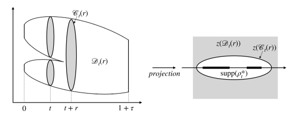
Figure 3: An illustration of the domain ${\mathcal{D}}_{t}(r)$, the contour $\mathscr{C}_{t}(r)$ , and their projections on the $z$-plane.

The bottom boundary of ${\mathcal{D}}_{t}(r)$ inside ${\mathcal{C}}_{t}^{+}$ is a curve, we denote it by $\mathscr{C}_{t}(r)$, and its projection on the $z$-plane as $z(\mathscr{C}_{t}(r))$. Then $z(\mathscr{C}_{t}(r))$ encloses $\operatorname{supp}(\rho_{t}^{*})$. Explicitly it is given

$$z(\mathscr{C}_{t}(r))=\{z=x-rf_{t+r}(x):(x,t+r)\in\Omega\}.$$ (6.26)

Thanks to Proposition 3.8, a neighborhood of $\operatorname{supp}(\rho_{t}^{*})$ is a bijection with its preimage under the projection map $(f_{t}(Z),z)\in{\mathcal{C}}_{t}^{+}\mapsto z\in{\mathbb{C}}$, i.e. for any $w$ in a neighborhood of $\operatorname{supp}(\rho_{t}^{*})$, the cardinality of $z^{-1}(w)$ is one. We can take ${\mathfrak{r}}>0$ small enough, such that for any $0\leqslant t\leqslant 1$, $z({\mathcal{C}}_{t}^{+}\setminus{\mathcal{D}}_{t}({\mathfrak{r}}))$ is inside such neighborhood of $\operatorname{supp}(\rho_{t}^{*})$. Then the projections $z({\mathcal{D}}_{t}({\mathfrak{r}})),z({\mathcal{C}}_{t}^{+}\setminus{\mathcal{D}}_{t}({\mathfrak{r}}))$ do not intersect with each other, $z({\mathcal{D}}_{t}({\mathfrak{r}}))\cap z({\mathcal{C}}_{t}^{+}\setminus{\mathcal{D}}_{t}({\mathfrak{r}}))=\emptyset$.

We define the following lattice on the domain ${\mathcal{D}}_{0}({\mathfrak{r}})$,

$$\mathcal{L}\mathrel{\mathop{:}}=\left\{z^{-1}(E+\mathrm{i}\eta)\in\operatorname{\mathcal{D}}_{0}({\mathfrak{r}}):E\in\mathbb{Z}/n^{2},\eta\in\mathbb{Z}/n^{2}\right\}.$$ (6.27)

It is easy to see from the characteristic flow (6.3), the image of the lattice ${\mathcal{L}}$ also gives a $1/n^{2}$ mesh of $Z_{t}({\mathcal{D}}_{0}({\mathfrak{r}}))$ after projected to the $z$-plane.

Proposition 6.6.

For any $0\leqslant t\leqslant 1$ and $W\in Z_{t}({\mathcal{D}}_{0}({\mathfrak{r}}))$, there exists some lattice point $Z\in\mathcal{L}$ as in (6.27), such that

$$|z_{t}(Z)-z(W)|\lesssim 1/n^{2}.$$

where the implicit constant depends on $\mu_{A}$.

By symmetry, in the rest of this section, we restrict ourselves in the subdomain that $\{Z\in{\mathcal{C}}_{0}:\mathop{\mathrm{Im}}[z(Z)]\geqslant 0\}$. In this case we have $\mathop{\mathrm{Im}}[f_{0}(Z)]\leqslant 0$, and for any $t\geqslant 0$ such that $Z_{t}(Z)\in{\mathcal{C}}_{t}^{+}$, $z_{t}(Z)$ remains nonnegative, i.e. $\mathop{\mathrm{Im}}[z_{t}(Z)]\geqslant 0$. The estimates for $\{Z\in{\mathcal{C}}_{0}:\mathop{\mathrm{Im}}[z(Z)]\leqslant 0\}$ follows by symmetry.

6.1 Short time estimates

Proposition 6.7.

Under the assumptions of Theorem 6.2, with high probability, the Stieltjes transform of the weighted nonintersecting Brownian bridge (4.8) satisfies the following estimates: with high probability, it holds uniformly for any $0\leqslant t\leqslant{\mathfrak{t}}_{0}$

$$\{x_{1}(t),x_{2}(t),\cdots,x_{n}(t)\}\in\cup_{k}[{\sf a}_{k}-{\mathfrak{C}}\sqrt{t}-\operatorname{o}(1),{\sf b}_{k}+{\mathfrak{C}}\sqrt{t}+\operatorname{o}(1)],$$ (6.28)

where $\mu_{A_{n}}$ is supported on $\cup_{k}[{\sf a}_{k}-\operatorname{o}(1),{\sf b}_{k}+\operatorname{o}(1)]$. As a consequence, $\operatorname{supp}\mu_{t}$ is contained in a ${\mathfrak{C}}\sqrt{t}+\operatorname{o}(1)$ neighborhood of $\operatorname{supp}\rho^{*}_{t}$.

We will need the following monotonicity statement for nonintersecting Brownian bridges, which follows directly from [17, Lemmas 2.6 and 2.7].

Theorem 6.8 ([17, Lemmas 2.6 and 2.7]).

Given two pairs of boundary data $(a_{1}\leqslant a_{2}\leqslant\cdots\leqslant a_{n})$, $(b_{1}\leqslant b_{2}\leqslant\cdots\leqslant b_{n})$, $(a^{\prime}_{1}\leqslant a^{\prime}_{2}\leqslant\cdots\leqslant a^{\prime}_{n})$ and $(b_{1}^{\prime}\leqslant b^{\prime}_{2}\leqslant\cdots\leqslant b^{\prime}_{n})$. We consider nonintersecting Brownian bridges from $(a_{1},a_{2},\cdots,a_{n})$ and $(a^{\prime}_{1},a^{\prime}_{2},\cdots,a^{\prime}_{n})$ to $(b_{1},b_{2},\cdots,b_{n})$ and $(b^{\prime}_{1},b^{\prime}_{2},\cdots,b^{\prime}_{n})$: $x_{1}(t)\leqslant x_{2}(t)\cdots\leqslant x_{n}(t)$ and $x^{\prime}_{1}(t)\leqslant x^{\prime}_{2}(t)\cdots\leqslant x^{\prime}_{n}(t)$. If $a_{i}\geqslant a^{\prime}_{i}$ and $b_{i}\geqslant b^{\prime}_{i}$ for all $1\leqslant i\leqslant n$, then there exists a coupling, such that at any time $0\leqslant t\leqslant 1$, $x_{i}(t)\geqslant x^{\prime}_{i}(t)$ for all $1\leqslant i\leqslant n$.

Proof of Proposition 6.7.

For weighted nonintersecting Brownian bridges (4.8) with boundary data $(a_{1}\leqslant a_{2}\leqslant\cdots\leqslant a_{n})$ and $(b_{1}\leqslant b_{2}\leqslant\cdots\leqslant b_{n})$, and $\mu_{A_{n}}$ is supported on $\cup_{k}[{\sf a}_{k}-\operatorname{o}(1),{\sf b}_{k}+\operatorname{o}(1)]$. We can take $a^{\prime}_{1}=a^{\prime}_{2}=\cdots=a_{n}^{\prime}=a_{1}={{\sf a}}_{1}-\operatorname{o}(1)\leqslant a_{1}$, and $b^{\prime}_{1}=b^{\prime}_{2}=\cdots=b^{\prime}_{n}=b_{1}$. Then the nonintersecting Brownian bridges $x^{\prime}_{1}(t)\leqslant x^{\prime}_{2}(t)\leqslant\cdots\leqslant x^{\prime}_{n}(t)$ is the well-understood Brownian watermelon (after an affine shift), and we have that with high probability $x^{\prime}_{1}(t)\geqslant{\sf a}_{0}-{\mathfrak{C}}\sqrt{t}+\operatorname{o}(1)$. Then Theorem 6.8 implies that $x_{1}(t)\geqslant x^{\prime}_{1}(t)\geqslant{\sf a}_{0}-{\mathfrak{C}}\sqrt{t}+\operatorname{o}(1)$. By the same argument we can show that

$$x_{i}(t)\leqslant{\sf b}_{k}+{\mathfrak{C}}\sqrt{t}+\operatorname{o}(1),\quad x_{i+1}(t)\leqslant{\sf a}_{k+1}-{\mathfrak{C}}\sqrt{t}+\operatorname{o}(1),\quad i=n\int_{-\infty}^{{\sf b}_{k}+\operatorname{o}(1)}{\rm d}\mu_{A_{n}},$$

and the claim 6.28 follows. ∎

Proposition 6.9.

Under the assumptions of Theorem 6.2, with high probability, the Stieltjes transform of the weighted nonintersecting Brownian bridge (4.8) satisfies the following estimates: for any $0\leqslant t\leqslant{\mathfrak{t}}_{0}$, and any $z\in{\mathbb{C}}_{+}$ outside the contour $z(\mathscr{C}_{t}({\mathfrak{r}}))$ as defined in (6.26), it holds for $z=z(Z)$

$$\left|\tilde{m}_{t}(z)-m_{t}(z)\right|\lesssim\frac{(\log n)^{{\mathfrak{a}}}}{n}.$$ (6.29)

We define the stopping time

$$\sigma\mathrel{\mathop{:}}=\inf_{t\geqslant 0}\left\{\exists W\in{\mathcal{D}}_{t}({\mathfrak{r}}):w=Z(W),\left|\Delta_{t}(w)\right|\geqslant\frac{{\mathfrak{M}}(t)}{n}\right\}\wedge{\mathfrak{t}}_{0},\quad{\mathfrak{M}}(t)\mathrel{\mathop{:}}={\mathfrak{C}}e^{{\mathfrak{C}}t}(\log n)^{{\mathfrak{a}}},$$ (6.30)

for some sufficiently large ${\mathfrak{C}}$, which we will choose later. We will prove that with high probability it holds that $\sigma={\mathfrak{t}}_{0}$. Then this implies that Proposition 6.9 holds for $z\in z({\mathcal{D}}_{t}({\mathfrak{r}}))$. For $z\not\in z({\mathcal{D}}_{t}({\mathfrak{r}}))$ and outside the contour $z(\mathscr{C}_{t}({\mathfrak{r}}))$, the estimate of the Stieltjes transform follows from a contour integral

$$\left|\tilde{m}_{t}(z)-m_{t}(z)\right|=\left|\frac{1}{2\pi\mathrm{i}}\oint_{z(\mathscr{C}_{t}({\mathfrak{r}}))}\frac{\tilde{m}_{t}(w)-m_{t}(w)}{z-w}{\rm d}w\right|\lesssim\frac{(\log n)^{{\mathfrak{a}}}}{n}.$$ (6.31)

For any $Z\in{\mathcal{L}}$ as in (6.27), we define $t(Z)$ to be the earliest time such that $Z_{t}(Z)$ no longer belongs to $\operatorname{\mathcal{D}}_{t}({\mathfrak{r}})$ up to ${\mathfrak{t}}_{0}$,

$$t(Z)\mathrel{\mathop{:}}=\sup_{s\geqslant 0}\{Z_{t}(Z)\in\operatorname{\mathcal{D}}_{t}({\mathfrak{r}})\}\wedge{\mathfrak{t}}_{0}.$$ (6.32)

Claim 6.10.

Under the assumptions of Theorem 6.2. There exists an event ${\mathcal{W}}$ that holds with high probability on which we have for every $Z\in\mathcal{L}$ as in (6.27) and $0\leqslant t\leqslant t(Z)\wedge\sigma$,

$$\left|\int_{0}^{t}{\rm d}{\mathcal{E}}_{2}(s)\right|\lesssim\frac{\log n}{n}.$$ (6.33)

Proof.

We have for any $0\leqslant t\leqslant t(Z)\wedge\sigma$, Proposition 6.7 implies that

$$\{x_{1}(t),x_{2}(t),\cdots,x_{n}(t)\}\in\cup_{k}[{\sf a}_{k}-{\mathfrak{C}}\sqrt{t}-\operatorname{o}(1),{\sf b}_{k}+{\mathfrak{C}}\sqrt{t}+\operatorname{o}(1)],$$ (6.34)

which is a small neighborhood of $\operatorname{supp}(\mu_{A})$. By taking ${\mathfrak{t}}_{0}$ sufficiently small and $n$ large enough, we can make sure that the righthand side of (6.34) is distance $\operatorname{O}(1)$ away from the contour $z(\mathscr{C}_{t}({\mathfrak{r}}))$. By the definition of $t(Z)$ as in (6.32), we have that $Z_{s}(Z)\in{\mathcal{D}}_{s}({\mathfrak{r}})$ for $0\leqslant s\leqslant t\leqslant t(Z)\wedge\sigma$. Especially $z_{s}(Z)$ is outside the contour $z(\mathscr{C}_{s}({\mathfrak{r}}))$. We conclude that

$$\operatorname{dist}(z_{s},\{x_{1}(s),x_{2}(s),\cdots,x_{n}(s)\})\gtrsim 1,\quad z_{s}=z_{s}(Z)$$ (6.35)

Then it follows that

$$\begin{split}&\left\langle\frac{1}{n^{3/2}}\int_{0}^{\cdot\wedge\sigma}\sum_{i=1}^{n}\frac{{\rm d}B_{i}(s)}{(x_{i}(s)-z_{s})^{2}}\right\rangle_{t}=\frac{1}{n^{3}}\int_{0}^{t\wedge\sigma}\sum_{i=1}^{n}\frac{{\rm d}s}{|x_{i}(s)-z_{s}|^{4}}\lesssim\frac{1}{n^{2}}.\end{split}$$

where we used (6.35). Therefore, by Burkholder-Davis-Gundy inequality, for any $Z\in\mathcal{L}$, the following holds with high probability, i.e., $1-n^{-{\mathfrak{C}}}$,

$$\begin{split}&\sup_{0\leqslant t\leqslant t(Z)}\left|\frac{1}{n^{3/2}}\int_{0}^{t\wedge\sigma}\sum_{i=1}^{n}\frac{{\rm d}B_{i}(s)}{(x_{i}(s)-z_{s})^{2}}\right|\lesssim\frac{\log n}{n}.\end{split}$$ (6.36)

We define ${\mathcal{W}}$ to be the set of Brownian paths $\{B_{1}(s),\cdots,B_{n}(s)\}_{0\leqslant s\leqslant{\mathfrak{t}}_{0}}$ on which (LABEL:eq:dd2term) holds for any $Z\in\mathcal{L}$. From the discussion above, ${\mathcal{W}}$ holds with overwhelming probability, i.e., $\mathbb{P}({\mathcal{W}})\geqslant 1-\operatorname{O}(|\mathcal{L}|n^{-{\mathfrak{C}}})$. This finishes the proof of Claim 6.10. ∎

We now bound the second term of (6.19).

Claim 6.11.

Under the assumptions of Theorem (6.2), for any $Z\in\mathcal{L}$ and $0\leqslant t\leqslant t(Z)\wedge\sigma$ as in (6.32), we have

$$\int\frac{g_{t}(x)-g_{t}(Z_{t})-(x-z_{t})\partial_{z}g_{t}(Z_{t})}{(z_{t}-x)^{2}}({\rm d}\mu_{t}-\rho_{t}^{*}(x){\rm d}x)\lesssim\frac{{\mathfrak{M}}(t)}{n},$$ (6.37)

where the implicit constant is independent of ${\mathfrak{M}}(t)$.

Proof.

We recall from (6.4), $g_{t}(Z)$ can be glued to an analytic function in a neighborhood of the bottom of ${\mathcal{C}}_{t}^{+}$, i.e. in a neighborhood of $\pi_{Q^{t}}(\{(x,t):x\in\operatorname{supp}(\rho_{t}^{*})\})$ and its complex conjugate. The integrand can also be extended to a meromorphic function on ${\mathcal{C}}_{t}^{+}$:

$$\frac{g_{t}(W)-g_{t}(Z_{t})-(z(W)-z_{t})\partial_{z}g_{t}(Z_{t})}{(z_{t}-z(W))^{2}},\quad W\in{\mathcal{C}}^{+}_{t}.$$ (6.38)

It only has poles at $\{W\in{\mathcal{C}}_{t}^{+}:W\neq Z_{t},z(W)=z_{t}\}$. By our choice of ${\mathcal{D}}_{t}({\mathfrak{r}})$, $z({\mathcal{C}}_{t}^{+}\setminus{\mathcal{D}}_{t}({\mathfrak{r}}))$ is a bijection with its preimage under the projection map $z:{\mathcal{C}}_{t}^{+}\mapsto{\mathbb{C}}$. So the poles of (6.38) are in ${\mathcal{D}}_{t}({\mathfrak{r}})$. Then we can take the contour $\mathscr{C}_{t}({\mathfrak{r}})$, whose projection on the $z$-plane encloses $\operatorname{supp}\mu_{t},\operatorname{supp}\rho_{t}^{*}$. We can rewrite (6.37) as a contour integral,

$$\frac{1}{2\pi\mathrm{i}}\oint_{\mathscr{C}_{t}({\mathfrak{r}})}\frac{g_{t}(W)-g_{t}(Z_{t})-(w-z_{t})\partial_{z}g_{t}(Z_{t})}{(z_{t}-w)^{2}}(\tilde{m}_{t}(w)-m_{t}(w)){\rm d}W,\quad w=z(W).$$

On the contour $\mathscr{C}_{t}({\mathfrak{r}})$, the integrand (6.38) is of order $\operatorname{O}(1)$, and our definition of the stopping time (6.30) implies that $|\tilde{m}_{t}(w)-m_{t}(w)|\leqslant{\mathfrak{M}}(t)/n$. It follows that

$$\left|\frac{1}{2\pi\mathrm{i}}\oint_{{\sf S}}\frac{g_{t}(W)-g_{t}(Z_{t})-(w-z_{t})\partial_{z}g_{t}(Z_{t})}{(z_{t}-w)^{2}}(\tilde{m}_{t}(w)-m_{t}(w)){\rm d}W\right|\lesssim\oint_{{\sf S}}\frac{{\mathfrak{M}}(t)}{n}|{\rm d}W|\lesssim\frac{{\mathfrak{M}}(t)}{n}.$$

The claim (6.37) follows. ∎

Claim 6.12.

Under the assumptions of Theorem (6.2), for any $Z\in\mathcal{L}$ and $0\leqslant t\leqslant t(Z)\wedge\sigma$ as in (6.32), we have

$$|(g_{t}(x_{i}(t);\mu_{t},t)-g_{t}(x_{i}(t))|\lesssim\frac{{\mathfrak{M}}(t)}{n}$$ (6.39)

and it follows that

$$\left|\frac{1}{n}\sum_{i=1}^{n}\frac{(g_{t}(x_{i}(t);\mu_{t},t)-g_{t}(x_{i}(t)))+{\mathcal{E}}^{(i)}_{t}({\bm{x}}(t))}{(z_{t}-x_{i}(t))^{2}}\right|\lesssim\frac{{\mathfrak{M}}(t)|\mathop{\mathrm{Im}}[\tilde{m}_{t}(z_{t})]|}{n\mathop{\mathrm{Im}}[z_{t}]},$$ (6.40)

where the implicit constant is independent of ${\mathfrak{M}}(t)$. When $\operatorname{dist}(z_{t},\{x_{1}(t),x_{2}(t),\cdots,x_{n}(t)\})\gtrsim 1$, the righthand side of (6.40) simplifies to $\operatorname{O}({\mathfrak{M}}(t)/n)$.

Proof.

To estimate (6.39) we interpolate the probability measures ${\rm d}\mu_{t}$ and $\rho_{t}^{*}(x){\rm d}x$

$${\rm d}\mu^{\theta}_{t}=\theta{\rm d}\mu_{t}+(1-\theta)\rho_{t}^{*}(x){\rm d}x,\quad 0\leqslant\theta\leqslant 1,$$

and write

$$g_{t}(x;\mu_{t},t)-g_{t}(x)=\int_{0}^{1}\partial_{\theta}g_{t}(x;\mu_{t}^{\theta},t){\rm d}\theta.$$

We recall that $g_{t}(x;\mu_{t}^{\theta},t)=f_{t}(x;\mu_{t}^{\theta},t)-\int 1/(x-y){\rm d}\mu_{t}^{\theta}(y)$. Using (3.6), we have

$$g_{t}(x;\mu_{t},t)-g_{t}(x)=\int_{0}^{1}\int\left(Q_{X_{\theta}(y),Z_{0}}(x;\mu_{t}^{\theta},t)-\frac{1}{y-x}\right)({\rm d}\mu_{t}(y)-\rho_{t}^{*}(y){\rm d}y){\rm d}\theta,$$ (6.41)

where $\{X_{\theta}(x)=(f_{t}(x;\mu^{\theta},t),x)\}_{x\in\operatorname{supp}(\mu^{\theta})}$. The integrand as a function of $y$, can be extended to a meromorphic function on ${\mathcal{C}}_{t}^{\mu_{t}^{\theta},t,+}$:

$$Q_{W,Z_{0}}(x;\mu_{t}^{\theta},t)-\frac{1}{z(W)-x},\quad W\in{\mathcal{C}}_{t}^{\mu_{t}^{\theta},t,+}.$$ (6.42)

More importantly, it glues to an analytic in a neighborhood of the bottom boundary of ${\mathcal{C}}_{t}^{\mu_{t}^{\theta},t,+}$. We can take a contour ${\sf S}$ over ${\mathcal{C}}_{t}^{\mu_{t}^{\theta},t,+}$, such that its projection encloses a neighborhood of $\operatorname{supp}\mu_{t},\operatorname{supp}\rho_{t}^{*}$, and is contained in $z({\mathcal{D}}_{t}({\mathfrak{r}}))$, and rewrite (6.41) as a contour integral,

$$\int_{0}^{1}\frac{1}{2\pi\mathrm{i}}\oint_{{\sf S}}\left(Q_{W,Z_{0}}(x;\mu_{t}^{\theta},t)-\frac{1}{z(W)-x}\right)(\tilde{m}_{t}(w)-m_{t}(w)){\rm d}W{\rm d}\theta,\quad w=z(W).$$

On the contour ${\sf S}$, the integrand (6.42) is of order $\operatorname{O}(1)$, and our definition of the stopping time (6.30) implies that $|\tilde{m}_{t}(w)-m_{t}(w)|\leqslant{\mathfrak{M}}(t)/n$. It follows that

$$\left|\int_{0}^{1}\frac{1}{2\pi\mathrm{i}}\oint_{{\sf S}}\left(Q_{W,Z_{0}}(x;\mu_{t}^{\theta},t)-\frac{1}{z(W)-x}\right)(\tilde{m}_{t}(w)-m_{t}(w)){\rm d}W{\rm d}\theta\right|\lesssim\int_{0}^{1}\oint_{{\sf S}}\frac{{\mathfrak{M}}(t)}{n}|{\rm d}W|{\rm d}\theta\lesssim\frac{{\mathfrak{M}}(t)}{n}.$$

The claim (6.39) follows.

For (6.40), using Proposition 5.2 and (6.39),

$$\left|\frac{1}{n}\sum_{i=1}^{n}\frac{(g_{t}(x_{i}(t);\mu_{t},t)-g_{t}(x_{i}(t)))+{\mathcal{E}}^{(i)}_{t}({\bm{x}}(t))}{(z_{t}-x_{i}(t))^{2}}\right|\lesssim\frac{1}{n}\sum_{i=1}^{n}\frac{{\mathfrak{M}}(t)/n+1/n^{2}}{|z_{t}-x_{i}(t)|^{2}}\lesssim\frac{{\mathfrak{M}}(t)|\mathop{\mathrm{Im}}[\tilde{m}_{t}(z_{t})]|}{n\mathop{\mathrm{Im}}[z_{t}]}.$$

This gives the claim (6.40). When $\operatorname{dist}(z_{t},\{x_{1}(t),x_{2}(t),\cdots,x_{n}(t)\})\gtrsim 1$, the above simplifies to $\operatorname{O}({\mathfrak{M}}(t)/n)$. ∎

We can now start analyzing (6.18). For any lattice point $Z\in\mathcal{L}$ and $0\leqslant t\leqslant t(Z)$ as in (6.32), by Claims 6.10, 6.11 and 6.12, we have

$$\left|\Delta_{t\wedge\sigma}(z_{t\wedge\sigma})\right|\lesssim|\Delta_{0}(z_{0})|+\int_{0}^{t\wedge\sigma}|\Delta_{s}(z_{s})||\partial_{z}\tilde{f}_{s}(Z_{s})|{\rm d}s+\frac{\log n}{n}+\int_{0}^{t\wedge\sigma}\frac{{\mathfrak{M}}(s){\rm d}s}{n}.$$ (6.43)

Notice that for $s\leqslant t\wedge\sigma$, we have $\left|\partial_{z}\tilde{f}_{s}(Z_{s})\right|\leqslant\left|\partial_{z}\tilde{m}_{s}(z_{s})\right|+\left|\partial_{z}g_{s}(Z_{s})\right|\lesssim 1$. Assumption 3.3 implies that $|\Delta_{0}(z_{0})|\lesssim(\log n)^{{\mathfrak{a}}}/n$. We can simplify (6.43) as

$$\left|\Delta_{t\wedge\sigma}(z_{t\wedge\sigma})\right|\lesssim\frac{(\log n)^{{\mathfrak{a}}}}{n}+\int_{0}^{t\wedge\sigma}\frac{{\mathfrak{M}}(s){\rm d}s}{n}.$$ (6.44)

We recall from (6.30), that ${\mathfrak{M}}(t)={\mathfrak{C}}e^{{\mathfrak{C}}t}(\log n)^{{\mathfrak{a}}}$. We can further simplify the righthand side of (6.44) and conclude that on the event ${\mathcal{W}}$,

$$\left|\Delta_{t\wedge\sigma}(z_{t\wedge\sigma})\right|\lesssim\frac{(1+e^{{\mathfrak{C}}(t\wedge\sigma)})(\log n)^{{\mathfrak{a}}}}{n}\leqslant\frac{{\mathfrak{C}}e^{{\mathfrak{C}}(t\wedge\sigma)}(\log n)^{{\mathfrak{a}}}}{2n},$$

provided ${\mathfrak{C}}$ is large enough. By Proposition 6.6, for any $W\in\operatorname{\mathcal{D}}_{t\wedge\sigma}({\mathfrak{r}})$ with $w=z(W)$, there exists some $Z\in\mathcal{L}$ such that $z_{t\wedge\sigma}(Z)\in\operatorname{\mathcal{D}}_{t\wedge\sigma}({\mathfrak{r}})$, and

$$|z_{t\wedge\sigma}(Z)-z(W)|\lesssim 1/n^{2}.$$

Moreover, on the domain $z(\mathcal{D}_{t\wedge\sigma}({\mathfrak{r}}))$, both $\tilde{m}_{t\wedge\sigma}$ and $m_{t\wedge\sigma}$ are Lipschitz with Lipschitz constant $\operatorname{O}(1)$. Therefore

$$\begin{split}&\phantom{{}={}}\left|\tilde{m}_{t\wedge\sigma}(w)-m_{t\wedge\sigma}(w)\right|\leqslant\left|\tilde{m}_{t\wedge\sigma}(z_{t\wedge\sigma}(Z))-m_{t\wedge\sigma}(z_{t\wedge\sigma}(Z))\right|\\ &+\left|\tilde{m}_{t\wedge\sigma}(w)-\tilde{m}_{t\wedge\sigma}(z_{t\wedge\sigma}(Z))\right|+\left|m_{t\wedge\sigma}(w)-m_{t\wedge\sigma}(z_{t\wedge\sigma}(Z))\right|\\ &\leqslant\frac{{\mathfrak{C}}e^{{\mathfrak{C}}(t\wedge\sigma)}(\log n)^{{\mathfrak{a}}}}{2n}+\operatorname{O}\left(\frac{1}{n^{2}}\right)\leqslant\frac{{\mathfrak{C}}e^{{\mathfrak{C}}(t\wedge\sigma)}(\log n)^{{\mathfrak{a}}}}{n}.\end{split}$$

It follows that $\sigma={\mathfrak{t}}_{0}$ and this completes the proof of Proposition 6.9.

6.2 Long time estimates

In this section, we prove Proposition 6.4 and (6.9). For them we need to understand the Stieltjes transform close to the spectrum. We define the following spectral domain as illustrated in Figure 4 :

$$\begin{split}{\mathcal{D}}_{t}^{\rm bulk}&=\left({\mathcal{D}}_{t}(\max\{{\mathfrak{r}}+({\mathfrak{t}}_{0}-t)/2,0\})\setminus{\mathcal{D}}_{t}(2{\mathfrak{r}})\right)\bigcap\\ &\{(f,z)\in{\mathcal{C}}_{t}^{+}:\operatorname{dist}(z,[{\sf a}(t),{\sf b}(t)])|\mathop{\mathrm{Im}}[f]|\wedge|\mathop{\mathrm{Im}}[z]|\geqslant(\log n)^{{\mathfrak{a}}+2}/n)\}.\end{split}$$ (6.45)

The estimates of Stieltjes transform on $\{(f,z)\in{\mathcal{C}}_{t}^{+}:\operatorname{dist}(z,[{\sf a}(t),{\sf b}(t)])|\mathop{\mathrm{Im}}[f]|\wedge|\mathop{\mathrm{Im}}[z]|\geqslant(\log n)^{{\mathfrak{a}}+2}/n)\}$ with $\mathop{\mathrm{Re}}[z]\in[{\sf a}(t),{\sf b}(t)]$ give the information of particles inside the bulk, and with $\mathop{\mathrm{Re}}[z]\notin[{\sf a}(t),{\sf b}(t)]$ can be used to control the locations of extreme particles.

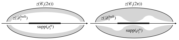
Figure 4: The projection of the spectral domain ${\mathcal{D}}_{t}^{\rm bulk}$ on the $z$-plane. The left subplot is the projection of ${\mathcal{D}}_{t}(\max\{{\mathfrak{r}}+({\mathfrak{t}}_{0}-t)/2,0\})\setminus{\mathcal{D}}_{t}(2{\mathfrak{r}})$ on the $z$-plane with ${\mathfrak{r}}+({\mathfrak{t}}_{0}-t)/2>0$. The right subplot is the projection of $\{(f,z)\in{\mathcal{C}}_{t}^{+}:\operatorname{dist}(z,[{\sf a}(t),{\sf b}(t)])|\mathop{\mathrm{Im}}[f]|\wedge|\mathop{\mathrm{Im}}[z]|\geqslant(\log n)^{{\mathfrak{a}}+2}/n)\}$ on the $z$-plane.

We recall the contours $\mathscr{C}_{t}(r)$ as defined in (6.26), which are the bottom boundary curves of ${\mathcal{D}}_{t}(r)$. For any $Z=(f,z)\in{\mathcal{C}}_{t}^{+}$, $f=m_{t}(z)+g_{t}(Z)$ (by (6.4)). Since $g_{t}(Z)$ is real for $z\in{\mathbb{R}}$, we have $|\mathop{\mathrm{Im}}[g_{t}(Z)]|=\operatorname{O}(\mathop{\mathrm{Im}}[z])\lesssim|\mathop{\mathrm{Im}}[m_{t}(z)]|$. Combining a contour integral similar to (6.31), the estimates on ${\mathcal{D}}_{t}^{\rm bulk}$ and ${\mathcal{D}}_{t}(2{\mathfrak{r}})$ give full information of the Stieltjes transform on

$$\{z\in{\mathbb{C}}:\operatorname{dist}(z,[{\sf a}(t),{\sf b}(t)])|\mathop{\mathrm{Im}}[m_{t}(z)]|\wedge|\mathop{\mathrm{Im}}[z]|\gtrsim(\log n)^{{\mathfrak{a}}+2}/n)\},$$

which is the domain in Proposition 6.4.

We recall from (6.26) that the curve $z(\mathscr{C}_{t}(r))$ is characterized by $\mathop{\mathrm{Im}}[z]+r\mathop{\mathrm{Im}}[f_{t}(z)]=0$, where $(f_{t}(z),z)\in{\mathcal{C}}_{t}^{+}$. Proposition 6.5 implies that for ${\mathfrak{t}}_{0}\leqslant t\leqslant 1$, the density $\rho_{t}^{*}$ has square root behavior. Thus $f_{t}(z)$ has square root behavior in a small neighborhood of ${\sf a}(t)$,

$$f_{t}(z)=f_{t}({\sf a}(t))+\Omega(1)\sqrt{{\sf a}(t)-z}+\operatorname{O}(|z-{\sf a}(t)|^{3/2})$$ (6.46)

where the square root is the branch with nonpositive imaginary part. Therefore, for $r\ll 1$, in a small neighborhood of ${\sf a}(t)$, if $z={\sf a}(s)-\kappa+\mathrm{i}\eta\in z(\mathscr{C}_{t}(r))$, solving $\mathop{\mathrm{Im}}[z]+r\mathop{\mathrm{Im}}[f_{t}(z)]=0$, we get that $\kappa+\eta\asymp r^{2}=\operatorname{o}(1)$ for $\kappa\geqslant 0$, and $\eta^{2}/(|\kappa|+\eta)\asymp r^{2}=\operatorname{o}(1)$ for $\kappa\leqslant 0$.

For any $Z\in{\mathcal{L}}$ as in (6.27), we define $t(Z)$ such that $Z_{t}(Z)$ no longer belong to $\operatorname{\mathcal{D}}_{t}^{\rm bulk}$ after time $t(Z)$:

$$t(Z)\mathrel{\mathop{:}}=\sup_{t\geqslant 0}\{Z_{t}(Z)\in{\mathcal{D}}_{t}(2{\mathfrak{r}})\cup{\mathcal{D}}_{t}^{\rm bulk}\}\wedge 1,$$ (6.47)

and the stopping time

$$\begin{split}\sigma&\mathrel{\mathop{:}}=\inf_{t\geqslant 0}\left\{\exists W\in{\mathcal{D}}_{t}(2{\mathfrak{r}}):w=z(W),\left|\Delta_{t}(w)\right|\geqslant\frac{{\mathfrak{M}}_{1}(t)}{n}\right\}\\ &\wedge\inf_{t\geqslant 0}\left\{\exists W\in{\mathcal{D}}_{t}^{\rm bulk}:w=z(W),\left|\Delta_{t}(w)\right|\geqslant\frac{{\mathfrak{C}}(\log n)^{{\mathfrak{a}}+1}}{n\sqrt{\mathop{\mathrm{Im}}[w]\operatorname{dist}(w,[{\sf a}(t),{\sf b}(t)])}}\right\}\wedge 1,\end{split}$$ (6.48)

for some sufficiently large ${\mathfrak{C}}$, which we will choose latter. Thanks to Proposition 6.9, on the event ${\mathcal{W}}$ as defined in Claim 6.10, we have that $\sigma\geqslant{\mathfrak{t}}_{0}$.

Claim 6.13.

Under the assumptions of Theorem 6.2, there exists a universal constant ${\mathfrak{C}}>0$ such that for any ${\mathfrak{t}}_{0}\leqslant t\leqslant 1$ and $Z\in{\mathcal{D}}_{0}({\mathfrak{r}})$ if $z_{t}(Z)={\sf a}(t)-\kappa_{t}(Z)+\mathrm{i}\eta_{t}(Z)$ and $\kappa_{t}(Z)\geqslant 0$, then for any ${\mathfrak{t}}_{0}\leqslant s\leqslant t$ either $\eta_{s}(Z)\gtrsim 1$, or $\kappa_{s}(Z)\gtrsim 1$, or

$$\partial_{s}\sqrt{\kappa_{s}(Z)}\leqslant-{\mathfrak{C}}\sqrt{\kappa_{s}(Z)+\eta_{s}(Z)}.$$ (6.49)

The same statement holds for characteristic flows close to the right edge. As a consequence if $Z_{t}(Z)\in{\mathcal{D}}_{t}^{\rm bulk}\cup{\mathcal{D}}_{t}(2{\mathfrak{r}})$, then $Z_{s}(Z)\in{\mathcal{D}}_{s}^{\rm bulk}\cup{\mathcal{D}}_{s}(2{\mathfrak{r}})$. If we further assume that ${\mathfrak{t}}_{0}\leqslant t\leqslant\sigma$ as defined in (6.48) and $Z_{t}(Z)\in{\mathcal{D}}_{t}^{\rm bulk}$, then we have

1. We denote

   $$\begin{split}&{\sf A}(t)\mathrel{\mathop{:}}={\sf a}(t)-(\log n)^{2{\mathfrak{a}}+4}/n^{2/3}\wedge\min\{E:E+\mathrm{i}\eta\in z(\mathscr{C}_{t}(\max\{{\mathfrak{r}}+({\mathfrak{t}}_{0}-t)/2,0\}))\},\\ &{\sf B}(t)\mathrel{\mathop{:}}={\sf b}(t)+(\log n)^{2{\mathfrak{a}}+4}/n^{2/3}\vee\max\{E:E+\mathrm{i}\eta\in z(\mathscr{C}_{t}(\max\{{\mathfrak{r}}+({\mathfrak{t}}_{0}-t)/2,0\}))\}.\end{split}$$ (6.50)

   The particles are all in the interval $[{\sf A}(t),{\sf B}(t)]$,

   $${\sf A}(t)\leqslant x_{1}(t)\leqslant x_{2}(t)\leqslant\cdots\leqslant x_{n}(t)\leqslant{\sf B}(t).$$ (6.51)

2. Let $z_{t}=z(Z_{t})$ the Stieltjes transform satisfies

   $$|\Delta_{t}(z_{t})|\lesssim(\log n)^{{\mathfrak{a}}+1}/(n\sqrt{\eta_{t}\operatorname{dist}(z_{t},[{\sf a}(t),{\sf b}(t)])})\lesssim\mathop{\mathrm{Im}}[m_{t}(z_{t})]/\log n.$$ (6.52)

3. For any ${\mathfrak{t}}_{0}\leqslant s\leqslant t$,

   $$\operatorname{dist}(z_{s}(Z),\{x_{1}(s),x_{2}(s),\cdots,x_{n}(s)\})\gtrsim\eta_{s}(Z)+\sqrt{\kappa_{s}(Z)+\eta_{s}(Z)}(t-s).$$ (6.53)

Proof.

The left edge ${\sf a}(s)$ of the density $\rho_{s}^{*}(x)$ is a critical point of $f_{s}$, which is characterized by $f_{s}^{\prime}({\sf a}(s))=\infty$ and satisfies the differential equation

$$\partial_{s}{\sf a}(s)=f_{s}({\sf a}(s)).$$ (6.54)

By taking difference between (6.54) and the characteristic flow $\partial_{s}z_{s}(Z)=f_{s}(z_{s}(Z))$, and then taking the real part we get

$$\partial_{s}\kappa_{s}=\mathop{\mathrm{Re}}[f_{s}({\sf a}_{s})-f_{s}(z_{s}(Z))].$$ (6.55)

There are several cases, either $\mathop{\mathrm{Im}}[z_{s}(Z)]\gtrsim 1$, then $\mathop{\mathrm{Im}}[z_{s^{\prime}}(Z)]\geqslant\mathop{\mathrm{Im}}[z_{s}(Z)]\gtrsim 1$ for all $0\leqslant s^{\prime}\leqslant s$; or $\kappa_{s}(Z)\gtrsim 1$; or $z_{s}(Z)$ is in a sufficiently small neighborhood of ${\sf a}(s)$. In this case, using the square root behavior (6.46) of $f_{t}(z)$, (6.55) implies that

$$\partial_{s}\kappa_{s}=\mathop{\mathrm{Re}}[f_{s}({\sf a}_{s})-f_{s}(z_{s}(Z))]\lesssim-\sqrt{\eta_{s}(Z)+\kappa_{s}(Z)}.$$ (6.56)

This gives (6.49).

If $Z_{t}(Z)\in{\mathcal{D}}_{t}^{\rm bulk}\cup{\mathcal{D}}_{t}(2{\mathfrak{r}})$, then $Z_{t}(Z)\in{\mathcal{D}}_{t}(\max\{{\mathfrak{r}}+({\mathfrak{t}}_{0}-t)/2,0\})$. By our construction (6.25) $Z_{s}(Z)\in{\mathcal{D}}_{s}(\max\{{\mathfrak{r}}+({\mathfrak{t}}_{0}-s)/2,0\})$. Moreover, since along the characteristic flow, for $s\leqslant r\leqslant t$, $\partial_{r}f_{r}(Z_{r})=0$, $\partial_{r}|\mathop{\mathrm{Im}}[z_{r}]|\leqslant 0$, and when $z_{r}={\sf a}(r)-\kappa_{r}(Z)+\mathrm{i}\eta_{r}(Z)$ with $\kappa_{r}(Z)\geqslant 0$ is in a small neighborhood of ${\sf a}(r)$, $\partial_{r}\sqrt{\kappa_{r}(Z)}\leqslant 0$ by (6.49). We conclude that $\operatorname{dist}(z_{s},[{\sf a}(s),{\sf b}(s)])|\mathop{\mathrm{Im}}[f_{s}(Z_{s})]|\wedge|\mathop{\mathrm{Im}}[z_{s}]|\geqslant(\log n)^{{\mathfrak{a}}+2}/n$, and $Z_{s}(Z)\in{\mathcal{D}}_{s}^{\rm bulk}\cup{\mathcal{D}}_{s}(2{\mathfrak{r}})$

The estimate (6.51) follows from estimates of the Stieltjes transform. More precisely, we take $\kappa\geqslant{\sf A}(t)-{\sf a}(A)\geqslant(\log n)^{2{\mathfrak{a}}+4}/n^{2/3}$ and $\eta=n^{-2/3}$. Then for $t\leqslant\sigma$, we have

$$|\tilde{m}_{t}({\sf a}(t)-\kappa+\mathrm{i}\eta)-m_{t}({\sf a}(t)-\kappa+\mathrm{i}\eta)|\lesssim\frac{(\log n)^{{\mathfrak{a}}+1}}{n\sqrt{\eta(\kappa+\eta)}}.$$ (6.57)

Thanks to the square root behavior of $m_{t}(z)$ from Proposition 6.5, $\mathop{\mathrm{Im}}[m_{t}({\sf a}(t)-\kappa+\mathrm{i}\eta)]\asymp\eta/\sqrt{\kappa+\eta}$. Thus we have

$$\tilde{m}_{t}({\sf a}(t)-\kappa+\mathrm{i}\eta)\lesssim\frac{\eta}{\sqrt{\kappa+\eta}}+\frac{(\log n)^{{\mathfrak{a}}+1}}{n\sqrt{\eta(\kappa+\eta)}}.$$ (6.58)

Thus by our choice take $\kappa\geqslant(\log n)^{2{\mathfrak{a}}+4}\eta$ and $\eta=n^{-2/3}$, (6.58) implies that $\mathop{\mathrm{Im}}[\tilde{m}_{t}({\sf a}(t)-\kappa+\mathrm{i}\eta)]\ll 1/n\eta$. However, if there exists a particle $x_{i}(t)$ such that $|x_{i}(t)-{\sf a}(t)+\kappa|\leqslant\eta$, we will have that

$$\mathop{\mathrm{Im}}[m_{t}({\sf a}(t)-\kappa+\mathrm{i}\eta)]=\frac{1}{n}\sum_{i=1}^{n}\frac{\eta}{(x_{i}(t)-\kappa-{\sf a}(t))^{2}+\eta^{2}}\geqslant\frac{1}{2n\eta}.$$ (6.59)

This leads to a contradiction. Since we can take any $\kappa\geqslant{\sf A}(t)-{\sf a}(t)$, we conclude that $x_{i}(t)\geqslant{\sf A}(t)$ for all $1\leqslant i\leqslant n$. The same argument implies that $x_{i}(t)\leqslant{\sf B}(t)$ for all $1\leqslant i\leqslant n$. This finishes the proof of (6.51).

The estimate (6.52) follows from the definition of the spectral domain ${\mathcal{D}}_{t}^{\rm bulk}$ as in (6.45).

For (6.53), since $\kappa_{t}(Z)\geqslant 0$, using (6.49), either $\eta_{s}(Z)\gtrsim 1$ or $\kappa_{s}(Z)\geqslant 0$. If $\eta_{s}(Z)\gtrsim 1$, (6.53) follows trivially,

$$\operatorname{dist}(z_{s}(Z),\{x_{1}(s),x_{2}(s),\cdots,x_{n}(s)\})\geqslant\eta_{s}(Z)\gtrsim 1\gtrsim\eta_{s}(Z)+\sqrt{\kappa_{s}(Z)+\eta_{s}(Z)}(t-s).$$

We consider the case that $\kappa_{s}(Z)\geqslant 0$. Using (6.51), we have

$$\operatorname{dist}(z_{s}(Z),\{x_{1}(s),x_{2}(s),\cdots,x_{n}(s)\})\geqslant\operatorname{dist}(z_{s}(Z),[{\sf A}(s),{\sf B}(s)])\geqslant\eta_{s}(Z).$$ (6.60)

We recall ${\sf A}(t)$ and ${\sf B}(t)$ from (LABEL:e:defsAB), and the behavior of the curve $z(\mathscr{C}_{t}(r))$ near ${\sf a}(t)$ from the discussion after (6.46). We take $r=\max\{{\mathfrak{r}}+({\mathfrak{t}}_{0}-s)/2,(\log n)^{{\mathfrak{a}}+2}/n^{1/3}\}$, then $[{\sf A}(s),{\sf B}(s)]$ is inside the contour $z(\mathscr{C}_{t}(r))$. Let $r^{\prime}$ to be such that $Z_{s}(Z)\in\mathscr{C}_{s}(r^{\prime})$. Then we have

$$\begin{split}\operatorname{dist}(z_{s}(Z),[{\sf A}(s),{\sf B}(s)])&\geqslant\operatorname{dist}(\{z\in z(\mathscr{C}_{s}(r^{\prime})):\mathop{\mathrm{Re}}[z]\leqslant{\sf a}(s)\},\{z\in z(\mathscr{C}_{s}(r)):\mathop{\mathrm{Re}}[z]\leqslant{\sf a}(s)\}).\end{split}$$ (6.61)

We have that $r^{\prime}\geqslant(t-s)/2+\max\{{\mathfrak{r}}+({\mathfrak{t}}_{0}-s)/2,(\log n)^{{\mathfrak{a}}+2}/n^{1/3}\}=(t-s)/2+r$.

If $r^{\prime}\gtrsim 1$, $\operatorname{dist}(\{z\in z(\mathscr{C}_{s}(r^{\prime})):\mathop{\mathrm{Re}}[z]\leqslant{\sf a}(s)\},{\sf a}(s))\gtrsim 1$. Moreover, since $f_{s}(z)$ is analytic away from the spectrum, in this case (6.61) implies

$$\begin{split}\operatorname{dist}(z_{s}(Z),[{\sf A}(s),{\sf B}(s)])&\geqslant\operatorname{dist}(\{z\in z(\mathscr{C}_{s}(r^{\prime})):\mathop{\mathrm{Re}}[z]\leqslant{\sf a}(s)\},\{z\in z(\mathscr{C}_{s}(r)):\mathop{\mathrm{Re}}[z]\leqslant{\sf a}(s)\})\\ &\gtrsim(r^{\prime}-r)\gtrsim(t-s)\gtrsim\sqrt{\kappa_{s}(Z)+\eta_{s}(Z)}(t-s).\end{split}$$ (6.62)

The claim (6.53) follows from combining (6.60) and (6.62).

If $r^{\prime}=\operatorname{o}(1)$, let $z={\sf a}(s)-\kappa+\mathrm{i}\eta\in z(\mathscr{C}_{s}(r^{\prime}))$, solving $\mathop{\mathrm{Im}}[z]+r^{\prime}\mathop{\mathrm{Im}}[f_{s}(z)]=0$, we get that $\kappa+\eta\asymp(r^{\prime})^{2}=\operatorname{o}(1)$. It follows that $r^{\prime}\asymp\sqrt{\kappa_{s}(Z)+\eta_{s}(Z)}$. Similarly, for any $z={\sf a}(s)-\kappa+\mathrm{i}\eta\in z(\mathscr{C}_{s}(r))$, we have that $\kappa+\eta\asymp r^{2}=\operatorname{o}(1)$. Thus (6.61) implies

$$\begin{split}\operatorname{dist}(z_{s}(Z),[{\sf A}(s),{\sf B}(s)])&\geqslant\operatorname{dist}(\{z\in z(\mathscr{C}_{s}(r^{\prime})):\mathop{\mathrm{Re}}[z]\leqslant{\sf a}(s)\},\{z\in z(\mathscr{C}_{s}(r)):\mathop{\mathrm{Re}}[z]\leqslant{\sf a}(s)\})\\ &\gtrsim r^{\prime}(r^{\prime}-r)\gtrsim(t-s)\sqrt{\kappa_{s}(Z)+\eta_{s}(Z)}.\end{split}$$ (6.63)

The claim (6.53) follows from combining (6.60) and (6.63).

∎

The following estimates on the integral of Stieltjes transform and characteristic flows will be used in later proofs.

Proposition 6.14.

Under the assumptions of Theorem 6.2, for any $Z\in{\mathcal{D}}_{0}({\mathfrak{r}})$, and $0\leqslant s\leqslant t\leqslant t(Z)$, let $z_{\tau}=z(Z_{\tau}(Z))$, then it holds

$$\int_{s}^{t}\frac{\mathop{\mathrm{Im}}[m_{\tau}(z_{\tau})]{\rm d}\tau}{\mathop{\mathrm{Im}}[z_{\tau}]}\leqslant{\mathfrak{C}}(t-s)+\log\frac{\mathop{\mathrm{Im}}[z_{s}]}{\mathop{\mathrm{Im}}[z_{t}]},\qquad\int_{s}^{t}\frac{\mathop{\mathrm{Im}}[m_{\tau}(z_{\tau})]{\rm d}\tau}{\mathop{\mathrm{Im}}[z_{\tau}]^{p}}\leqslant\frac{{\mathfrak{C}}}{\mathop{\mathrm{Im}}[z_{t}]^{p-1}},\quad p>1$$ (6.64)

Proof.

For (6.64) we have

$$\int_{s}^{t}\frac{\mathop{\mathrm{Im}}[m_{\tau}(z_{\tau})]{\rm d}\tau}{\mathop{\mathrm{Im}}[z_{\tau}]^{p}}=\int_{s}^{t}\frac{\mathop{\mathrm{Im}}[f_{\tau}(Z_{\tau})-g_{\tau}(Z_{\tau})]{\rm d}\tau}{\mathop{\mathrm{Im}}[z_{\tau}]^{p}}\leqslant\int_{s}^{t}\frac{\partial_{\tau}\mathop{\mathrm{Im}}[z_{\tau}]}{\mathop{\mathrm{Im}}[z_{\tau}]^{p}}+\int_{s}^{t}\frac{{\mathfrak{C}}{\rm d}\tau}{\mathop{\mathrm{Im}}[z_{\tau}]^{p-1}}$$

where we used that $\mathop{\mathrm{Im}}[g_{\tau}(Z_{\tau})]\lesssim\mathop{\mathrm{Im}}[z_{\tau}]$, and $f_{\tau}(Z_{\tau})=\partial_{\tau}z_{\tau}$. The claim (6.64) follows. ∎

Claim 6.15.

Under the assumptions of Theorem 6.2, there exists an event ${\mathcal{W}}$ with high probability, such that on ${\mathcal{W}}$ we have for every $Z\in\mathcal{L}$ and $0\leqslant t\leqslant\sigma$, if $z_{t}(Z)\in{\mathcal{D}}_{t}(2{\mathfrak{r}})$ then

$$\left|\int_{0}^{t}{\rm d}{\mathcal{E}}_{2}(s)\right|\lesssim\frac{\log n}{n};$$ (6.65)

if $z_{t}(Z)\in{\mathcal{D}}_{t}^{\rm bulk}$ then

$$\left|\int_{0}^{t}{\rm d}{\mathcal{E}}_{2}(s)\right|\lesssim\frac{\log n}{n\sqrt{\mathop{\mathrm{Im}}[z_{t}(Z)]\operatorname{dist}(z_{t}(Z),[{\sf a}(t),{\sf b}(t)])}},$$ (6.66)

where $\rho_{t}^{*}$ is surppored on $[{\sf a}(t),{\sf b}(t)]$

Proof.

If $z_{t}(Z)\in{\mathcal{D}}_{t}(2{\mathfrak{r}})$, the $z_{s}(Z)\in{\mathcal{D}}_{s}(2{\mathfrak{r}})$ for any $0\leqslant s\leqslant t$, and we have $\operatorname{dist}(z_{s}(Z),\{x_{1}(s),x_{2}(s),\cdots,x_{n}(s)\})\gtrsim 1$ from (6.51). The first claim (6.65) follows from the same argument as in Claim 6.10.

For (6.66), there are two cases i) $\operatorname{dist}(z_{t}(Z),[{\sf a}(t),{\sf b}(t)])\leqslant\mathop{\mathrm{Im}}[z_{t}(Z)]$, then the righthand side of (6.66) simplifies to $\operatorname{O}(\log n/n\mathop{\mathrm{Im}}[z_{t}(Z)])$. ii) $\operatorname{dist}(z_{t}(Z),[{\sf a}(t),{\sf b}(t)])\geqslant\mathop{\mathrm{Im}}[z_{t}(Z)]$, then it is necessary that $\mathop{\mathrm{Re}}[z_{t}(Z)]\not\in\operatorname{supp}(\rho_{t}^{*})$. Without loss of generality, we assume that $\operatorname{dist}(z_{t}(Z),\operatorname{supp}(\rho_{t}^{*}))$ is achieved at the left edge ${\sf a}(t)$ of $\rho_{t}^{*}$. Then we can write $z_{t}(Z)={\sf a}(t)-\kappa_{t}(Z)+\mathrm{i}\eta_{t}(Z)$, with $\kappa_{t}(Z)\geqslant 0$, and the righthand side of (6.66) simplifies to $\operatorname{O}(\log n/n\sqrt{\eta_{t}(Z)(\kappa_{t}(Z)+\eta_{t}(Z))})$.

In the first case that $\operatorname{dist}(z_{t}(Z),[{\sf a}(t),{\sf b}(t)])\leqslant\mathop{\mathrm{Im}}[z_{t}(Z)]$, we decompose the time interval $[0,t]$ in the following way. First we set $t_{0}=0$, and define

$$t_{i+1}(Z):=\sup_{s\geqslant t_{i}(Z)}\left\{\mathop{\mathrm{Im}}[z_{s}(Z)]\geqslant\frac{\mathop{\mathrm{Im}}[z_{t_{i}}(Z)]}{2}\right\}\wedge t,\quad i=0,1,2,\cdots.$$

From our choice of domain ${\mathcal{D}}_{t}^{\rm bulk}$, $\mathop{\mathrm{Im}}[z_{0}(Z)]/\mathop{\mathrm{Im}}[z_{t}(Z)]\lesssim n$. The above sequence will terminate at some $t_{k}(Z)=t$ for $k=\operatorname{O}(\log n)$ depending on $Z$. Moreover, since $\mathop{\mathrm{Im}}[z_{s}(Z)]$ is monotone decreasing for any $t_{i}(Z)\leqslant t\leqslant t_{i+1}(Z)$,

$$\mathop{\mathrm{Im}}[z_{t_{i}}(Z)]\leqslant\mathop{\mathrm{Im}}[z_{t}(Z)]\leqslant\mathop{\mathrm{Im}}[z_{t_{i+1}}(Z)]\leqslant 2\mathop{\mathrm{Im}}[z_{t_{i}}(Z)].$$ (6.67)

Then it follows that

$$\begin{split}&\left\langle\frac{1}{n^{3/2}}\int_{0}^{\cdot\wedge\sigma}\sum_{i=1}^{n}\frac{{\rm d}B_{i}(s)}{(x_{i}(s)-z_{s}(Z))^{2}}\right\rangle_{t_{i}}=\frac{1}{n^{3}}\int_{0}^{t_{i}\wedge\sigma}\sum_{i=1}^{n}\frac{{\rm d}s}{|x_{i}(s)-z_{s}(Z)|^{4}}\\ \leqslant&\frac{1}{n^{3}}\int_{0}^{t_{i}\wedge\sigma}\sum_{i=1}^{n}\frac{{\rm d}s}{\mathop{\mathrm{Im}}[z_{s}(Z)]^{2}|x_{i}(s)-z_{s}(Z)|^{2}}\leqslant\int_{0}^{t_{i}\wedge\sigma}\frac{\mathop{\mathrm{Im}}[\tilde{m}_{s}(z_{s}(Z))]{\rm d}s}{n^{2}\mathop{\mathrm{Im}}[z_{s}(Z)]^{3}}\\ \lesssim&\int_{0}^{t_{i}\wedge\sigma}\frac{\mathop{\mathrm{Im}}[m_{s}(z_{s}(Z))]{\rm d}s}{n^{2}\mathop{\mathrm{Im}}[z_{s}(Z)]^{3}}\lesssim\frac{1}{n^{2}\mathop{\mathrm{Im}}[z_{t_{i}\wedge\sigma}(Z)]^{2}},\end{split}$$

where we used (6.52) and (6.64). Therefore, by Burkholder-Davis-Gundy inequality, for any $Z\in\mathcal{L}$ and $t_{i}$, the following holds with high probability, i.e., $1-n^{-{\mathfrak{C}}}$,

$$\begin{split}&\sup_{0\leqslant t\leqslant t_{i}}\left|\frac{1}{n^{3/2}}\int_{0}^{t\wedge\sigma}\sum_{i=1}^{n}\frac{{\rm d}B_{i}(s)}{(x_{i}(s)-z_{s}(Z))^{2}}\right|\lesssim\frac{\log n}{n\mathop{\mathrm{Im}}[z_{t_{i}\wedge\sigma}(Z)]}.\end{split}$$ (6.68)

Moreover, for any $t\in[t_{i-1},t_{i}]$, the bound (LABEL:eq:2term0) and (6.67) yield

$$\begin{split}\left|\int_{0}^{t\wedge\sigma}{\rm d}{\mathcal{E}}_{2}(s)\right|\lesssim&\frac{\log n}{n\mathop{\mathrm{Im}}[z_{t_{i}\wedge\sigma}(Z)]}\lesssim\frac{\log n}{n\mathop{\mathrm{Im}}[z_{t\wedge\sigma}(Z)]}.\end{split}$$ (6.69)

where we used (6.67).

For the second case that $z_{t}(Z)={\sf a}(t)-\kappa_{t}(Z)+\mathrm{i}\eta_{t}(Z)$, with $\kappa_{t}(Z)\geqslant 0$. We decompose the time interval $[0,t]$ in the following way. First we set $t_{0}(Z)=0$, and define

$$t_{i+1}(Z):=\sup_{s\geqslant t_{i}(Z)}\left\{\eta_{s}(Z)(\kappa_{s}(Z)+\eta_{s}(Z))\geqslant\frac{\eta_{t_{i}}(Z)(\kappa_{t_{i}}(Z)+\eta_{t_{i}}(Z))}{2}\right\}\wedge t,\quad i=0,1,2,\cdots.$$ (6.70)

Since $\eta_{t}(Z)\geqslant n^{-2/3}$ and $\eta_{0}(Z),\kappa_{0}(Z)\lesssim 1$, we have $t_{k}(Z)=t$ for $k=\operatorname{O}(\log n)$. We compute the quadratic variance of ${\rm d}{\mathcal{E}}_{2}(s)$,

$$\begin{split}&\phantom{{}={}}\left\langle\frac{1}{n^{3/2}}\int_{0}^{\cdot\wedge\sigma}\sum_{i=1}^{n}\frac{{\rm d}B_{i}(s)}{(x_{i}(s)-z_{s})^{2}}\right\rangle_{t_{i}}=\frac{1}{n^{3}}\int_{0}^{t_{i}\wedge\sigma}\sum_{i=1}^{n}\frac{{\rm d}s}{|x_{i}(s)-z_{s}|^{4}}\\ &\leqslant\frac{1}{n^{3}}\int_{0}^{t_{i}\wedge\sigma}\sum_{i=1}^{n}\frac{{\rm d}s}{\operatorname{dist}(z_{s},\{x_{j}(s)\}_{1\leqslant j\leqslant n})^{2}|x_{i}(s)-z_{s}|^{2}}=\frac{1}{n^{2}}\int_{0}^{t_{i}\wedge\sigma}\frac{\mathop{\mathrm{Im}}[\tilde{m}_{s}(z_{s})]{\rm d}s}{\operatorname{dist}(z_{s},\{x_{j}(s)\}_{1\leqslant j\leqslant n})^{2}\eta_{s}}\\ &\lesssim\frac{1}{n^{2}}\int_{0}^{t_{i}\wedge\sigma}\frac{\mathop{\mathrm{Im}}[m_{s}(z_{s})]}{\eta_{s}((\kappa_{s}+\eta_{s})^{1/2}(t_{i}-s)+\eta_{s})^{2}}{\rm d}s\lesssim\frac{1}{n^{2}}\int_{0}^{t_{i}\wedge\sigma}\frac{\eta_{s}/{\sqrt{\kappa_{s}+\eta_{s}}}}{\eta_{s}((\kappa_{s}+\eta_{s})^{1/2}(t_{i}-s)+\eta_{s})^{2}}{\rm d}s\\ &\lesssim\frac{1}{n^{2}}\int_{0}^{t_{i}\wedge\sigma}\frac{{\rm d}s}{(\kappa_{s}+\eta_{s})^{3/2}(t_{i}-s+\eta_{s}/(\kappa_{s}+\eta_{s})^{1/2})^{2}}\\ &\leqslant\frac{1}{n^{2}}\int_{0}^{t_{i}\wedge\sigma}\frac{{\rm d}s}{(\kappa_{t_{i}\wedge\sigma}+\eta_{t_{i}\wedge\sigma})^{3/2}(t_{i}-s+\eta_{t_{i}\wedge\sigma}/(\kappa_{t_{i}\wedge\sigma}+\eta_{t_{i}\wedge\sigma})^{1/2})^{2}}\lesssim\frac{1}{n^{2}}\frac{1}{\eta_{t_{i}\wedge\sigma}(\kappa_{t_{i}\wedge\sigma}+\eta_{t_{i}\wedge\sigma})},\end{split}$$

where in the third line we used (6.24), (6.52) and (6.53), in the fifth line we used that

$$\frac{\eta_{s}}{\sqrt{\kappa_{s}+\eta_{s}}}\asymp\mathop{\mathrm{Im}}[m_{s}(z_{s})]\asymp\mathop{\mathrm{Im}}[f_{s}(z_{s})]=\mathop{\mathrm{Im}}[f_{t_{i}\wedge\sigma}(z_{t_{i}\wedge\sigma})]\asymp\mathop{\mathrm{Im}}[m_{t_{i}\wedge\sigma}(z_{t_{i}\wedge\sigma})]\asymp\frac{\eta_{t_{i}\wedge\sigma}}{\sqrt{\kappa_{t_{i}\wedge\sigma}+\eta_{t_{i}\wedge\sigma}}}.$$

Therefore, by Burkholder-Davis-Gundy inequality, for any $Z\in{\mathcal{L}}$ and $t_{i}(Z)$, the following holds with high probability, i.e., $1-n^{-{\mathfrak{C}}}$,

$$\begin{split}&\sup_{0\leqslant t\leqslant t_{i}}\left|\frac{1}{n^{3/2}}\int_{0}^{t\wedge\sigma}\sum_{i=1}^{n}\frac{{\rm d}B_{i}(s)}{(x_{i}(s)-z_{s}(Z))^{2}}\right|\lesssim\frac{\log n}{n\sqrt{\eta_{t_{i}\wedge\sigma}(Z)(\kappa_{t_{i}\wedge\sigma}(Z)+\eta_{t_{i}\wedge\sigma}(Z))}}.\end{split}$$ (6.71)

Moreover, for any $t\in[t_{i-1},t_{i}]$, the bound (LABEL:eq:2term) with (6.70) yield

$$\begin{split}\left|\int_{0}^{t\wedge\sigma}{\rm d}{\mathcal{E}}_{2}(s)\right|\lesssim&\frac{\log n}{n\sqrt{\eta_{t_{i}\wedge\sigma}(Z)(\kappa_{t_{i}\wedge\sigma}(Z)+\eta_{t_{i}\wedge\sigma}(Z))}}\lesssim\frac{\log n}{n\sqrt{\eta_{t\wedge\sigma}(Z)(\kappa_{t\wedge\sigma}(Z)+\eta_{t\wedge\sigma}(Z))}}.\end{split}$$ (6.72)

We define ${\mathcal{W}}$ to be the set of Brownian paths $\{B_{1}(s),\cdots,B_{n}(s)\}_{0\leqslant s\leqslant t}$ on which (6.65), (6.69) and (6.72) hold for any $Z\in{\mathcal{L}}$ and times $t_{0}(Z),t_{1}(Z),t_{2}(Z)\cdots$. The above discussions imply that ${\mathcal{W}}$ holds with overwhelming probability, i.e., $\mathbb{P}({\mathcal{W}})\geqslant 1-\operatorname{O}(\log n|{\mathcal{L}}|n^{-{\mathfrak{C}}})$. This finishes the proof of Claim 6.15. ∎

With Proposition 6.9 as input, we can now start to prove Proposition 6.4.

Proof of Proposition 6.4.

For $z\in{\mathbb{C}}_{+}$ outside the contour $z(\mathscr{C}_{t}(2{\mathfrak{r}}))$, the estimate (6.10) follows from the same argument as Proposition 6.9. In the following we prove (6.10) for $z$ close to the spectrum. We notice that the Claims 6.10, 6.11 and 6.12 still hold for any $Z\in{\mathcal{L}}$ with new $t(Z)$ and stoping time $\sigma$ defined in (6.47) and (6.48) respectively. Moreover, for any $Z\in{\mathcal{L}}$, Assumption 3.3 implies that $|\Delta_{0}(z_{0})|\lesssim(\log n)^{{\mathfrak{a}}}/n$. Thus, for $Z\in{\mathcal{L}}$ with $z_{t}(Z)\in{\mathcal{D}}_{t}^{\rm bulk}$, we can write (6.18) as

$$|\Delta_{t\wedge\sigma}(z_{t\wedge\sigma})|\leqslant\int_{0}^{t\wedge\sigma}|\Delta_{s}(z_{s})||\partial_{z}\tilde{f}_{s}(Z_{s}){\rm d}s|+\operatorname{O}\left(\frac{(\log n)^{{\mathfrak{a}}}}{n\sqrt{\mathop{\mathrm{Im}}[z_{t\wedge\sigma}]\operatorname{dist}(z_{t\wedge\sigma},[{\sf a}(t\wedge\sigma),{\sf b}(t\wedge\sigma)])}}\right).$$ (6.73)

For the integrand of (6.73), we notice that for $s\leqslant t\wedge\sigma$,

$$\begin{split}\left|\partial_{z}\tilde{f}_{s}(Z_{s})\right|&\leqslant\left|\partial_{z}\tilde{m}_{s}(z_{s})\right|+\left|\partial_{z}g_{s}(Z_{s})\right|\leqslant\frac{\mathop{\mathrm{Im}}[\tilde{m}_{s}(z_{s})]}{\mathop{\mathrm{Im}}[z_{s}]}+\operatorname{O}(1)\\ &=\frac{\mathop{\mathrm{Im}}[\tilde{f}_{s}(Z_{s})-g_{s}(Z_{s})]}{\mathop{\mathrm{Im}}[z_{s}]}+\operatorname{O}(1)\leqslant\frac{\mathop{\mathrm{Im}}[\tilde{f}_{s}(Z_{s})]}{\mathop{\mathrm{Im}}[z_{s}]}+\operatorname{O}(1),\end{split}$$ (6.74)

where we used that $g_{s}(Z)$ is real for $z=z(Z)\in{\mathbb{R}}$, and thus $\mathop{\mathrm{Im}}[g_{s}(Z_{s})]=\operatorname{O}(\mathop{\mathrm{Im}}[z_{s}])$. Since $z_{s}(Z)\in\mathcal{D}^{\rm bulk}_{s}$, by the definition of $\mathcal{D}^{\rm bulk}_{s}$, we have $\mathop{\mathrm{Im}}[f_{s}(Z_{s})]\geqslant(\log n)^{{\mathfrak{a}}+2}/(n\mathop{\mathrm{Im}}[z_{s}])$. Moreover, since $s\leqslant\sigma$, we have $|\tilde{f}_{s}(Z_{s})-f_{s}(Z_{s})|=|\Delta_{s}(z_{s})|\lesssim(\log n)^{{\mathfrak{a}}+1}/(n\mathop{\mathrm{Im}}[z_{s}])\lesssim\mathop{\mathrm{Im}}[f_{s}(Z_{s})]/\log n$. Therefore,

$$\begin{split}\left|\partial_{z}\tilde{f}_{s}(Z_{s})\right|&\leqslant\frac{\mathop{\mathrm{Im}}[\tilde{f}_{s}(Z_{s})]}{\mathop{\mathrm{Im}}[z_{s}]}+\operatorname{O}(1)\leqslant\frac{\mathop{\mathrm{Im}}[f_{s}(Z_{s})]+|\Delta_{s}(z_{s})|}{\mathop{\mathrm{Im}}[z_{s}]}+\operatorname{O}(1)\\ &=\left(1+\frac{\operatorname{O}(1)}{\log n}\right)\frac{\mathop{\mathrm{Im}}[f_{s}(Z_{s})]}{\mathop{\mathrm{Im}}[z_{s}(u)]}+\operatorname{O}(1)=\left(1+\frac{\operatorname{O}(1)}{\log n}\right)\frac{\partial_{s}\mathop{\mathrm{Im}}[z_{s}]}{\mathop{\mathrm{Im}}[z_{s}]}+\operatorname{O}(1).\end{split}$$ (6.75)

We denote

$$\beta_{s}\mathrel{\mathop{:}}=\left|\partial_{z}\tilde{f}_{s}(Z_{s})\right|=\left(1+\frac{\operatorname{O}(1)}{\log n}\right)\frac{\partial_{s}\mathop{\mathrm{Im}}[z_{s}]}{\mathop{\mathrm{Im}}[z_{s}]}+\operatorname{O}(1)=\operatorname{O}\left(\frac{\partial_{s}\mathop{\mathrm{Im}}[z_{s}]}{\mathop{\mathrm{Im}}[z_{s}]}\right).$$ (6.76)

With $\beta_{s}$, we can rewrite (6.73) as

$$\begin{split}\left|\Delta_{t\wedge\sigma}(z_{t\wedge\sigma})\right|\leqslant\int_{0}^{t\wedge\sigma}\beta_{s}\left|\Delta_{s}(z_{s})\right|{\rm d}s+\operatorname{O}\left(\frac{(\log n)^{{\mathfrak{a}}}}{n\sqrt{\mathop{\mathrm{Im}}[z_{t\wedge\sigma}]\operatorname{dist}(z_{t\wedge\sigma},[{\sf a}(t\wedge\sigma),{\sf b}(t\wedge\sigma)])}}\right).\end{split}$$

By Grönwall’s inequality, this implies the estimate

$$\begin{split}\left|\Delta_{t\wedge\sigma}(z_{t\wedge\sigma})\right|&\lesssim\frac{(\log n)^{{\mathfrak{a}}}}{n\sqrt{\mathop{\mathrm{Im}}[z_{t\wedge\sigma}]\operatorname{dist}(z_{t\wedge\sigma},[{\sf a}(t\wedge\sigma),{\sf b}(t\wedge\sigma)])}}\\ &+\int_{0}^{t\wedge\sigma}\beta_{s}e^{\int_{s}^{t\wedge\sigma}\beta_{\tau}{\rm d}\tau}\frac{(\log n)^{{\mathfrak{a}}}}{n\sqrt{\mathop{\mathrm{Im}}[z_{s}]\operatorname{dist}(z_{s},[{\sf a}(s),{\sf b}(s)])}}{\rm d}s.\end{split}$$ (6.77)

For the integral of $\beta_{\tau}$, we have

$$e^{\int_{s}^{t\wedge\sigma}\beta_{\tau}{\rm d}\tau}\leqslant e^{\operatorname{O}(t-s)}e^{\left(1+\frac{\operatorname{O}(1)}{\log n}\right)\log\left(\frac{\mathop{\mathrm{Im}}[z_{s}(u)]}{\mathop{\mathrm{Im}}[z_{t\wedge\sigma}(u)]}\right)}=e^{\operatorname{O}(t-s)}\left(\frac{\mathop{\mathrm{Im}}[z_{s}(u)]}{\mathop{\mathrm{Im}}[z_{t\wedge\sigma}(u)]}\right)^{1+\frac{\operatorname{O}(1)}{\log n}}\leqslant\operatorname{O}(1)\frac{\mathop{\mathrm{Im}}[z_{s}(u)]}{\mathop{\mathrm{Im}}[z_{t\wedge\sigma}(u)]}.$$

In the last inequality, we used that by our construction of ${\mathcal{D}}_{t}^{\rm bulk}$, we have $\mathop{\mathrm{Im}}[z_{s}(u)]/\mathop{\mathrm{Im}}[z_{t\wedge\sigma}(u)]=\operatorname{O}(n)$. Combining the above inequality with (6.76) we can bound the last term in (6.77) by

$$\begin{split}&\phantom{{}={}}\int_{0}^{t\wedge\sigma}\beta_{s}e^{\int_{s}^{t\wedge\sigma}\beta_{\tau}{\rm d}\tau}\frac{(\log n)^{{\mathfrak{a}}}}{n\sqrt{\mathop{\mathrm{Im}}[z_{s}]\operatorname{dist}(z_{s},[{\sf a}(s),{\sf b}(s)])}}{\rm d}s\\ &\lesssim\int_{0}^{t\wedge\sigma}\frac{\partial_{s}\mathop{\mathrm{Im}}[z_{s}]}{\mathop{\mathrm{Im}}[z_{t\wedge\sigma}]}\frac{(\log n)^{{\mathfrak{a}}}}{n\sqrt{\mathop{\mathrm{Im}}[z_{s}]\operatorname{dist}(z_{s},[{\sf a}(s),{\sf b}(s)])}}{\rm d}s\\ &\lesssim\frac{(\log n)^{{\mathfrak{a}}}}{n\mathop{\mathrm{Im}}[z_{t\wedge\sigma}(u)]}\int_{0}^{t\wedge\sigma}\frac{\partial_{s}\mathop{\mathrm{Im}}[z_{s}]}{\sqrt{\mathop{\mathrm{Im}}[z_{s}]\operatorname{dist}(z_{s},[{\sf a}(s),{\sf b}(s)])}}{\rm d}s.\end{split}$$ (6.78)

There are two cases i) $\operatorname{dist}(z_{t\wedge\sigma}(Z),[{\sf a}({t\wedge\sigma}),{\sf b}({t\wedge\sigma})])\leqslant\mathop{\mathrm{Im}}[z_{t\wedge\sigma}(Z)]$. ii)$\operatorname{dist}(z_{t\wedge\sigma}(Z),[{\sf a}({t\wedge\sigma}),{\sf b}({t\wedge\sigma})])\geqslant\mathop{\mathrm{Im}}[z_{t\wedge\sigma}(Z)]$, then it is necessary that $\mathop{\mathrm{Re}}[z_{t\wedge\sigma}(Z)]\not\in\operatorname{supp}(\rho_{t\wedge\sigma}^{*})$. Without loss of generality, we assume that $\operatorname{dist}(z_{t\wedge\sigma}(Z),\operatorname{supp}(\rho_{t\wedge\sigma}^{*}))$ is achieved at the left edge ${\sf a}_{1}({t\wedge\sigma})$ of $\rho_{t\wedge\sigma}^{*}$. Then we can write $z_{t\wedge\sigma}(Z)={\sf a}({t\wedge\sigma})-\kappa_{t\wedge\sigma}(Z)+\mathrm{i}\eta_{t\wedge\sigma}(Z)$, with $\kappa_{t\wedge\sigma}(Z)\geqslant 0$, and $\operatorname{dist}(z_{t\wedge\sigma}(Z),{\sf a}({t\wedge\sigma}))\asymp\kappa_{t}(Z)+\eta_{t}(Z)$.

In the first case, using (6.64) we have

$$\begin{split}\int_{0}^{t\wedge\sigma}\frac{\partial_{s}\mathop{\mathrm{Im}}[z_{s}]}{\sqrt{\mathop{\mathrm{Im}}[z_{s}]\operatorname{dist}(z_{s},[{\sf a}(s),{\sf b}(s)])}}{\rm d}s\lesssim\int_{0}^{t\wedge\sigma}\frac{\partial_{s}\mathop{\mathrm{Im}}[z_{s}]}{\mathop{\mathrm{Im}}[z_{s}]}{\rm d}s=\log\left(\frac{\mathop{\mathrm{Im}}[z_{0}]}{\mathop{\mathrm{Im}}[z_{t\wedge\sigma}]}\right)\lesssim\log n,\end{split}$$ (6.79)

It follows by combining (6.77), (LABEL:e:term2) and (6.79), we get that

$$\left|\Delta_{t\wedge\sigma}(z_{t\wedge\sigma})\right|\lesssim\frac{(\log n)^{{\mathfrak{a}}+1}}{n\mathop{\mathrm{Im}}[z_{t\wedge\sigma}]}\leqslant\frac{{\mathfrak{C}}(\log n)^{{\mathfrak{a}}+1}}{2n\sqrt{z_{t\wedge\sigma}\operatorname{dist}(z_{t\wedge\sigma}(Z),[{\sf a}({t\wedge\sigma}),{\sf b}({t\wedge\sigma})])}},$$ (6.80)

provided we take ${\mathfrak{C}}$ large enough.

In the second case, we can bound the last term in (6.77) by

$$\begin{split}&\int_{0}^{t\wedge\sigma}\frac{\partial_{s}\mathop{\mathrm{Im}}[z_{s}]}{\sqrt{\mathop{\mathrm{Im}}[z_{s}]\operatorname{dist}(z_{s},[{\sf a}(s),{\sf b}(s)])}}{\rm d}s\lesssim\int_{0}^{t\wedge\sigma}\frac{\partial_{s}\eta_{s}}{\sqrt{\eta_{s}(\kappa_{s}+\eta_{s})}}{\rm d}s\\ &\lesssim\frac{\eta_{t\wedge\sigma}}{\sqrt{\eta_{t\wedge\sigma}+\kappa_{t\wedge\sigma}}}\int_{0}^{t\wedge\sigma}\frac{\partial_{s}\eta_{s}}{(\eta_{s})^{3/2}}{\rm d}s\lesssim\frac{\sqrt{\eta_{t\wedge\sigma}}}{\sqrt{\eta_{t\wedge\sigma}+\kappa_{t\wedge\sigma}}},\end{split}$$ (6.81)

It follows by combining (6.77), (LABEL:e:term2) and (LABEL:e:term3), we get that

$$\left|\Delta_{t\wedge\sigma}(z_{t\wedge\sigma})\right|\lesssim\frac{(\log n)^{{\mathfrak{a}}}}{n\sqrt{\eta_{t\wedge\sigma}(\eta_{t\wedge\sigma}+\kappa_{t\wedge\sigma})}}\leqslant\frac{{\mathfrak{C}}(\log n)^{{\mathfrak{a}}+1}}{2n\sqrt{z_{t\wedge\sigma}\operatorname{dist}(z_{t\wedge\sigma}(Z),[{\sf a}({t\wedge\sigma}),{\sf b}({t\wedge\sigma})])}},$$ (6.82)

provided we take ${\mathfrak{C}}$ large enough.

Similarly to the proof of Proposition 6.4, we can approximate $W\in{\mathcal{D}}_{t\wedge\sigma}^{\rm bulk}$ with $w=z(W)$, by the image of some lattice point $Z\in{\mathcal{L}}$. And on the domain ${\mathcal{D}}_{t\wedge\sigma}^{\rm bulk}$, we also have that both both $\tilde{m}_{t\wedge\sigma}$ and $m_{t\wedge\sigma}$ are Lipschitz with Lipschitz constant $\operatorname{O}(n)$. Therefore (6.80) and (6.82) imply

$$\begin{split}&\phantom{{}={}}\left|\tilde{m}_{t\wedge\sigma}(w)-m_{t\wedge\sigma}(w)\right|\leqslant\frac{{\mathfrak{C}}(\log n)^{{\mathfrak{a}}+1}}{n\mathop{\mathrm{Im}}[z_{t\wedge\sigma}]},\end{split}$$

uniformly for $w\in z({\mathcal{D}}_{t\wedge\sigma}^{\rm bulk})$. It follows that $\sigma=1$, and this finishes the proof of Proposition 6.4.

∎

7 Optimal particle rigidity for nonintersecting Brownian bridges

In Theorem 6.2, we have proved the Optimal particle rigidity for the weighted nonintersecting Brownian bridges. In this section, using a coupling argument, we show the optimal particle rigidity for nonintersecting Brownian bridges with fixed boundary data.

Theorem 7.1.

Under Assumptions 3.1, 3.2, 3.3 and 3.4, for any small time ${\mathfrak{t}}>0$, the following holds for the particle locations of nonintersecting Brownian bridges between $\mu_{A_{n}}$ and $\mu_{B_{n}}$. With high probability, for any time ${\mathfrak{t}}\leqslant t\leqslant 1$ we have

1. We denote $\gamma_{i}(t)$ the $1/n$-quantiles of the density $\rho^{*}_{t}(\cdot)$, i.e.

   $$\frac{i+1/2}{n}=\int_{-\infty}^{\gamma_{i}(t)}\rho_{t}^{*}(x){\rm d}x,\quad 1\leqslant i\leqslant n,$$

   then uniformly for $1\leqslant i\leqslant n$, the locations of $x_{i}(t)$ are close to their corresponding quantiles

   $$\gamma_{i-(\log n)^{\operatorname{O}(1)}}(t)\leqslant x_{i}(t)\leqslant\gamma_{i+(\log n)^{\operatorname{O}(1)}}(t).$$ (7.1)

2. If $\rho_{t}^{*}$ is supported on $[{\sf a}(t),{\sf b}(t)]$, then the particles close to the left and right boundary points of $\operatorname{supp}(\rho_{t}^{*})$ satisfies

   $$x_{1}(t)\geqslant{\sf a}(t)-\frac{(\log n)^{\operatorname{O}(1)}}{n^{2/3}},\quad x_{n}(t)\leqslant{\sf b}(t)+\frac{(\log n)^{\operatorname{O}(1)}}{n^{2/3}}.$$ (7.2)

Proof.

We recall from (4.8), the weighted nonintersecting Brownian bridges (4.8) can be sampled in two steps. First we sample the boundary ${\bm{b}}^{\prime}=(b_{1}^{\prime},b_{2}^{\prime},\cdots,b_{n}^{\prime})$ using the density (4.9). Then we sample nonintersecting Brownian bridges with boundary data ${\bm{a}},{\bm{b}}^{\prime}$. Under Assumptions 3.1, 3.2 and 3.3, in Theorem 6.2, we showed that for any time ${\mathfrak{t}}\leqslant t\leqslant 1$, the particles of the weighted nonintersecting Brownian bridges satisfy optimal rigidity estimates. As an easy consequence, there exists a boundary data ${\bm{b}}^{\prime}$ (sampled from the density (4.9)), it satisfies:

$$\gamma_{i-(\log n)^{\operatorname{O}(1)}}(1)\leqslant b_{i}^{\prime}\leqslant\gamma_{i+(\log n)^{\operatorname{O}(1)}}(1).$$

and

$$b^{\prime}_{1}\geqslant{\sf a}(1)-\frac{(\log n)^{\operatorname{O}(1)}}{n^{2/3}},\quad b^{\prime}_{n}\leqslant{\sf b}(1)+\frac{(\log n)^{\operatorname{O}(1)}}{n^{2/3}}.$$

Moreover, the nonintersecting Brownian bridges between ${\bm{a}},{\bm{b}}^{\prime}$ satisfies the optimal rigidity estimates as in Theorem 6.2.

We denote the nonintersecting Brownian bridges between ${\bm{a}}$ and ${\bm{b}}^{\prime}$ as $\{y_{1}(t)\leqslant y_{2}(t)\leqslant\cdots\leqslant y_{n}(t)\}_{0\leqslant t\leqslant 1}$. Then with high probability, it holds

$$\gamma_{i-(\log n)^{\operatorname{O}(1)}}(t)\leqslant y_{i}(t)\leqslant\gamma_{i+(\log n)^{\operatorname{O}(1)}}(t).$$ (7.3)

If $\rho_{t}^{*}$ is supported on $[{\sf a}(t),{\sf b}(t)]$, then the particles close to the left and right boundary points of $\operatorname{supp}(\rho_{t}^{*})$ satisfies

$$y_{1}(t)\geqslant{\sf a}(t)-\frac{(\log n)^{\operatorname{O}(1)}}{n^{2/3}},\quad y_{n}(t)\leqslant{\sf b}(t)+\frac{(\log n)^{\operatorname{O}(1)}}{n^{2/3}}.$$ (7.4)

Since $b_{i}\leqslant b^{\prime}_{i+(\log n)^{\operatorname{O}(1)}}$, and $a_{i}\leqslant a_{i+(\log n)^{\operatorname{O}(1)}}$, using the monotonicity of nonintersecting brownian bridges, Theorem 6.8, we can couple the nonintersecting Brownian bridges $\{x_{1}(t)\leqslant x_{2}(t)\leqslant\cdots\leqslant x_{n}(t)\}_{0\leqslant t\leqslant 1}$ and $\{y_{1}(t)\leqslant y_{2}(t)\leqslant\cdots\leqslant y_{n}(t)\}_{0\leqslant t\leqslant 1}$,

$$x_{i}(t)\leqslant y_{i+(\log n)^{\operatorname{O}(1)}},\quad 0\leqslant t\leqslant 1,$$ (7.5)

where we used the convention that $y_{i}=+\infty$ for $i>n$. The coupling (7.5) and (7.3) together implies

$$x_{i}(t)\leqslant y_{i+(\log n)^{\operatorname{O}(1)}}(t)\leqslant\gamma_{i+(\log n)^{\operatorname{O}(1)}},\quad{\mathfrak{t}}\leqslant t\leqslant 1,$$ (7.6)

with high probability. A similar coupling using $b_{i}\geqslant b^{\prime}_{i-(\log n)^{\operatorname{O}(1)}}$ and $a_{i}\geqslant a_{i-(\log n)^{\operatorname{O}(1)}}$ implies

$$x_{i}(t)\geqslant y_{i-(\log n)^{\operatorname{O}(1)}}(t)\geqslant\gamma_{i-(\log n)^{\operatorname{O}(1)}},\quad{\mathfrak{t}}\leqslant t\leqslant 1,$$ (7.7)

where we used the convention that $y_{i}=-\infty$ for $i\leqslant 0$. The claim (7.1) follows from combining (7.6) and (7.7).

To prove (7.2), we construct the new boundary data:

$${\bm{b}}^{\pm}=(b^{\prime}_{1}\pm(\log n)^{{\mathfrak{C}}}n^{-2/3},b^{\prime}_{2}\pm(\log n)^{{\mathfrak{C}}}n^{-2/3},\cdots,b^{\prime}_{n}\pm(\log n)^{{\mathfrak{C}}}n^{-2/3}).$$ (7.8)

Thanks to Assumption 3.4, if we take ${\mathfrak{C}}$ large enough, then

$$b_{i}^{-}\leqslant b_{i},b_{i}^{\prime}\leqslant b_{i}^{+},\quad 1\leqslant i\leqslant n.$$

Since affine shifts preserve nonintersecting Brownian bridges, the nonintersecting Brownian bridges between ${\bm{a}}$ and ${\bm{b}}^{\pm}$, denoted as $y_{1}^{\pm}(t)\leqslant y^{\pm}_{2}(t)\leqslant\cdots\leqslant y^{\pm}_{n}(t)$, they can be coupled with the nonintersecting Brownian bridge $y_{1}(t)\leqslant y_{2}(t)\leqslant\cdots\leqslant y_{n}(t)$

$$y_{i}^{-}(t)=y_{i}(t)-\frac{t(\log n)^{{\mathfrak{C}}}}{n^{2/3}},\quad y_{i}^{+}(t)=y_{i}(t)+\frac{t(\log n)^{{\mathfrak{C}}}}{n^{2/3}},\quad 0\leqslant t\leqslant 1.$$

Thanks to Theorem 6.2, it holds with high probability,

$${\sf a}(t)-\frac{(\log n)^{\operatorname{O}(1)}}{n^{2/3}}\leqslant y_{1}^{-}(t)\leqslant y_{1}^{+}(t)\leqslant y_{n}^{-}(t)\leqslant y_{n}^{+}(t)\leqslant{\sf b}(t)+\frac{(\log n)^{\operatorname{O}(1)}}{n^{2/3}},\quad 0\leqslant t\leqslant 1.$$

Using the monotonicity of nonintersecting brownian bridges, Theorem 6.8, we can couple the nonintersecting Brownian bridges $x_{1}(t)\leqslant x_{2}(t)\leqslant\cdots\leqslant x_{n}(t)$ with the nonintersecting Brownian bridges $\{y_{1}^{\pm}(t)\leqslant y^{\pm}_{2}(t)\leqslant\cdots\leqslant y^{\pm}_{n}(t)\}_{t_{0}\leqslant t\leqslant 1}$, and conclude that with high probability

$${\sf a}(t)-\frac{(\log n)^{\operatorname{O}(1)}}{n^{2/3}}\leqslant y_{1}^{-}(t)\leqslant x_{1}(t)\leqslant x_{n}(t)\leqslant y_{n}^{+}(t)\leqslant{\sf b}(t)+\frac{(\log n)^{\operatorname{O}(1)}}{n^{2/3}},\quad{\mathfrak{t}}\leqslant t\leqslant 1.$$ (7.9)

This finishes the proof of (7.2).

∎

8 Edge Universality

In this section we prove edge universality for nonintersecting Brownian bridges Theorem 1.1. The proof consists of two parts. In Section 8.1, we prove the edge universality for the weighted nonintersecting Brownian bridges (4.8). The edge universality for nonintersecting Brownian bridges follows from a coupling with weighted nonintersecting Brownian bridges. The proof is given in Section 8.2.

8.1 Edge Universality for weighted nonintersecting Brownian bridges

We recall the random walk corresponding to the weighted nonintersecting Brownian bridges from (4.13)

$${\rm d}x_{i}(t)=\frac{1}{\sqrt{n}}{\rm d}B_{i}(t)+\frac{1}{n}\sum_{j:j\neq i}\frac{{\rm d}t}{x_{i}(t)-x_{j}(t)}+g_{t}(x_{i}(t),\mu_{t},t)+{\mathcal{E}}_{t}^{(i)}({\bm{x}}(t)).$$ (8.1)

In this section we prove edge universality for the weighted nonintersecting Brownian bridges (8.1). We recall from (3.6), for any $0<t<1$, in the neighborhood of $x={\sf a}(t)$, the limiting density $\rho_{t}^{*}(x)$ has square root behavior

$$\rho_{t}^{*}(x)=\frac{{\sf s}(t)\sqrt{[x-{\sf a}(t)]_{+}}}{\pi}+\operatorname{O}(|x-{\sf a}(t)|^{3/2}).$$ (8.2)

Proposition 8.1.

Fix small ${\mathfrak{t}}>0$. Under the Assumptions 3.1, 3.2 and 3.3 as $n$ goes to infinity, the fluctuations of extreme particles of the weighted nonintersecting Brownian bridges (8.1) after proper rescaling, converge to the Airy point process: for any time ${\mathfrak{t}}\leqslant t\leqslant 1$, the

$$({\sf s}(t)n)^{2/3}(x_{1}(t)-{\sf a}(t),x_{2}(t)-{\sf a}(t),x_{3}(t)-{\sf a}(t),\cdots)\rightarrow\text{Airy Point Process}$$

The same statement holds for particles close to the right edge.

Under Assumptions 3.1, 3.2 and 3.3, in Theorem 6.2, we showed that for any time ${\mathfrak{t}}\leqslant t\leqslant 1$, the particles of the random walk (8.1) satisfy optimal rigidity estimates. Fix time ${\mathfrak{t}}_{0}={\mathfrak{t}}-n^{-1/3+\operatorname{o}(1)}$, we can condition on the weighted nonintersecting Brownian bridge (8.1) at time ${\mathfrak{t}}_{0}$, such that ${\bm{x}}({\mathfrak{t}}_{0})$ satisfies the optimal rigidity estimates. Then from Claim 6.12, we have that with high probability for any ${\mathfrak{t}}_{0}\leqslant t\leqslant 1$, $g_{t}(x_{i}(t),\mu_{t},t)=g_{t}(x_{i}(t))+\operatorname{O}(\log n/n)$, and we can rewrite (8.1) as

$${\rm d}x_{i}(t)=\frac{1}{\sqrt{n}}{\rm d}B_{i}(t)+\frac{1}{n}\sum_{j:j\neq i}\frac{{\rm d}t}{x_{i}(t)-x_{j}(t)}+g_{t}(x_{i}(t))+\operatorname{O}\left(\frac{\log n}{n}\right).$$ (8.3)

The error term $\operatorname{O}(\log n/n)$ does not affect edge fluctuation, which is on the scale $\operatorname{O}(n^{-2/3})$. If we ignore the error term, (8.3) is the Dyson’s Brownian motion with drift $g_{t}(\cdot)$. For Dyson’s Brownian motion with general drift, the short time edge universality is well-understood.

In [1], joint with A. Adhikari, we considered the $\beta$-Dyson’s Brownian motion with general potential $V$,

$${\rm d}y_{i}(t)=\sqrt{\frac{2}{\beta n}}{\rm d}B_{i}(t)+\frac{1}{n}\sum_{j:j\neq i}\frac{{\rm d}t}{y_{i}(t)-y_{j}(t)}-\frac{1}{2}V^{\prime}(y_{i}(t)){\rm d}t,\quad i=1,2,\cdots,n.$$ (8.4)

For any probability density $\rho_{0}$, we denote $\rho_{t}$ the solution of the McKean-Vlasov equation [1, Equation (2.2)] associated to (8.4) with initial data $\rho_{0}$. If the initial data of the Dyson’s Brownian motion (8.4), weakly converges to $\rho_{0}$, then the empirical particle density of (8.4) at time $t\geqslant 0$ weakly converges to $\rho_{t}$. Moreover, if $\rho_{0}$ has square root behavior in a small neighborhood of its left edge, i.e. $\rho_{0}(x)=S(0)\sqrt{[x-E(0)]_{+}}/\pi+\operatorname{O}(|x-E(0)|^{3/2})$, then $\rho_{t}$ also has square root behavior, $\rho_{t}(x)=S(t)\sqrt{[x-E(t)]_{+}}/\pi+\operatorname{O}(|x-E(t)|^{3/2})$.

One result of [1] states that the extreme particles of the Dyson’s Brownian motion for general $\beta$ and potential $V$ converge to the Airy-$\beta$ point process in a short time.

Theorem 8.2.

[1, Theorem 6.1] Suppose the potential $V$ is analytic, and near the left edge the initial data of (8.4) satisfies rigidity estimates on the optimal scale $(\log n)^{\operatorname{O}(1)}/n^{2/3}$ with respect to a measure $\rho_{0}$, which has square root behavior in a small neighborhood of its left edge . Let $t\asymp N^{-1/3+\operatorname{o}(1)}$, then with high probability,

$$(S(t)n)^{2/3}(y_{1}(t)-E(t),y_{2}(t)-E(t),y_{3}(t)-E(t),\cdots)\rightarrow\text{Airy-$\beta$ Point Process}.$$

The same statement holds for particles close to the right edge.

Although the potential for the $\beta$-Dyson’s Brownian motion (8.4) studied in [1] does not depend on time. It is straightforward to adapt the proof in [1] for the case that the potential smoothly depends on time. Proposition 8.1 follows from applying Theorem 8.2 to (8.3).

8.2 Edge Universality for nonintersecting Brownian bridge

In this section we prove the main result of this paper Theorem 1.1, edge universality of nonintersecting Brownian bridges.

Proof of Theorem 1.1.

Fix time $t_{0}\leqslant t$ such that $n^{-2/3+\operatorname{o}(1)}\leqslant t-t_{0}\ll(\log n)^{-{\mathfrak{C}}}$, where the constant ${\mathfrak{C}}$ will be chosen later. We construct the new boundary data:

$${\bm{b}}^{\pm}=(b_{1}\pm(\log n)^{{\mathfrak{C}}}n^{-2/3},b_{2}\pm(\log n)^{{\mathfrak{C}}}n^{-2/3},\cdots,b_{n}\pm(\log n)^{{\mathfrak{C}}}n^{-2/3}),$$ (8.5)

with ${\mathfrak{C}}$ large enough, such that

$$b_{i}^{-}\leqslant b_{i}\leqslant b_{i}^{+},\quad 1\leqslant i\leqslant n.$$

We denote nonintersecting Brownian bridges between ${\bm{a}}$ and ${\bm{b}}$ after conditioning on time $t_{0}$, as $\{x_{1}(s)\leqslant x_{2}(s)\leqslant\cdots\leqslant x_{n}(s)\}_{t_{0}\leqslant s\leqslant 1}$. The affine shifts preserve nonintersecting Brownian bridges. If we denote the nonintersecting Brownian bridges between $x_{1}(t_{0})\leqslant x_{2}(t_{0})\leqslant\cdots\leqslant x_{n}(t_{0})$, and ${\bm{b}}^{\pm}$, as $x_{1}^{\pm}(s)\leqslant x^{\pm}_{2}(s)\leqslant\cdots\leqslant x^{\pm}_{n}(s)$, we can couple it with the nonintersecting Brownian bridges between ${\bm{a}}$ and ${\bm{b}}$

$$x_{i}^{-}(s)=x_{i}(s)-\frac{s-t_{0}}{1-t_{0}}\frac{(\log n)^{{\mathfrak{C}}}}{n^{2/3}},\quad x_{i}^{+}(s)=x_{i}(s)+\frac{s-t_{0}}{1-t_{0}}\frac{(\log n)^{{\mathfrak{C}}}}{n^{2/3}},\quad t_{0}\leqslant s\leqslant 1$$

Especially, at time $s=t$ with $t-t_{0}\ll(\log n)^{-{\mathfrak{C}}}$, it holds that

$$x_{i}^{-}(t),x_{i}^{+}(t)=x_{i}(t)+\operatorname{o}(n^{-2/3})$$ (8.6)

We denote $\{y_{1}(s)\leqslant y_{2}(s)\leqslant\cdots\leqslant y_{n}(s)\}_{t_{0}\leqslant s\leqslant 1}$ the weighted nonintersecting Brownian bridges starting at time $t_{0}$ with initial data $x_{1}(t_{0})\leqslant x_{2}(t_{0})\leqslant\cdots\leqslant x_{n}(t_{0})$. Then the same argument as in Proposition 8.1 gives that at time $s=t$, the extreme particles of $\{y_{1}(t)\leqslant y_{2}(t)\leqslant\cdots\leqslant y_{n}(t)\}$ are asymptotically given by Airy point process,

$$({\sf s}(t)n)^{2/3}(y_{1}(t)-{\sf a}(t),y_{2}(t)-{\sf a}(t),y_{3}(t)-{\sf a}(t),\cdots)\rightarrow\text{Airy Point Process}.$$ (8.7)

Moreover, Theorem 6.2 implies that with high probability $y_{i}(1)$ is close to the corresponding $1/n$-quantiles of the density $\rho_{B}$, as defined in (6.7)

$$\gamma_{i-(\log n)^{\operatorname{O}(1)}}(1)\leqslant y_{i}(1)\leqslant\gamma_{i+(\log n)^{\operatorname{O}(1)}}(t),$$ (8.8)

and the particles close to the left and right boundary points of $\operatorname{supp}(\rho_{B})$ satisfies

$$y_{1}(t)\geqslant{\sf a}(1)-\frac{(\log n)^{\operatorname{O}(1)}}{n^{2/3}},\quad y_{n}(t)\leqslant{\sf b}(1)+\frac{(\log n)^{\operatorname{O}(1)}}{n^{2/3}}.$$ (8.9)

Thanks to Assumption 3.4, if we take ${\mathfrak{C}}$ large enough, then with high probability

$$b_{i}^{-}\leqslant y_{i}(1)\leqslant b_{i}^{+}.$$

Using the monotonicity of nonintersecting Brownian bridges, Theorem 6.8, we can couple the the weighted nonintersecting Brownian bridges starting at time $t_{0}$ with initial data $x_{1}(t_{0})\leqslant x_{2}(t_{0})\leqslant\cdots\leqslant x_{n}(t_{0})$ with the nonintersecting Brownian bridges $\{x_{1}^{\pm}(s)\leqslant x^{\pm}_{2}(s)\leqslant\cdots\leqslant x^{\pm}_{n}(s)\}_{t_{0}\leqslant s\leqslant 1}$, and conclude that with high probability

$$x_{i}^{-}(s)\leqslant y_{i}(s)\leqslant x_{i}^{+}(s).$$ (8.10)

Estimates (8.6) and (8.10) imply that with high probability at time $s=t$ with $t-t_{0}\ll(\log n)^{-{\mathfrak{C}}}$,

$$y_{i}(t)=x_{i}(t)+\operatorname{o}(n^{-2/3}).$$ (8.11)

Theorem 1.1 follows from combining (8.7) and (8.11). ∎

References

- [1] A. Adhikari and J. Huang. Dyson brownian motion for general and potential at the edge. Probability Theory and Related Fields, pages 1–58, 2020.
- [2] M. Adler, J. Delépine, and P. Van Moerbeke. Dyson’s nonintersecting brownian motions with a few outliers. Communications on Pure and Applied Mathematics: A Journal Issued by the Courant Institute of Mathematical Sciences, 62(3):334–395, 2009.
- [3] M. Adler, P. L. Ferrari, P. Van Moerbeke, et al. Airy processes with wanderers and new universality classes. The Annals of Probability, 38(2):714–769, 2010.
- [4] M. Adler, P. L. Ferrari, P. Van Moerbeke, et al. Nonintersecting random walks in the neighborhood of a symmetric tacnode. The Annals of Probability, 41(4):2599–2647, 2013.
- [5] M. Adler and P. Van Moerbeke. PDEs for the gaussian ensemble with external source and the pearcey distribution. Communications on Pure and Applied Mathematics: A Journal Issued by the Courant Institute of Mathematical Sciences, 60(9):1261–1292, 2007.
- [6] M. Adler, P. van Moerbeke, and D. Vanderstichelen. Non-intersecting brownian motions leaving from and going to several points. Physica D: Nonlinear Phenomena, 241(5):443–460, 2012.
- [7] A. I. Aptekarev, P. M. Bleher, and A. B. Kuijlaars. Large n limit of gaussian random matrices with external source, part ii. Communications in mathematical physics, 259(2):367–389, 2005.
- [8] S. Belinschi, A. Guionnet, and J. Huang. Large deviation principles via spherical integrals. preprint, arXiv:2004.07117, 2020.
- [9] S. Bergman and M. Schiffer. Kernel functions and conformal mapping. Compositio Math., 8:205–249, 1951.
- [10] P. Biane. On the free convolution with a semi-circular distribution. Indiana Univ. Math. J., 46(3):705–718, 1997.
- [11] P. Biane, P. Bougerol, N. O’Connell, et al. Littelmann paths and brownian paths. Duke Mathematical Journal, 130(1):127–167, 2005.
- [12] P. Bleher and A. B. Kuijlaars. Large n limit of gaussian random matrices with external source, part i. Communications in mathematical physics, 252(1-3):43–76, 2004.
- [13] P. M. Bleher and A. B. Kuijlaars. Large n limit of gaussian random matrices with external source, part iii: double scaling limit. Communications in mathematical physics, 270(2):481–517, 2007.
- [14] E. Brézin and S. Hikami. Level spacing of random matrices in an external source. Physical Review E, 58(6):7176, 1998.
- [15] E. Brézin and S. Hikami. Universal singularity at the closure of a gap in a random matrix theory. Physical Review E, 57(4):4140, 1998.
- [16] I. Corwin. The kardar–parisi–zhang equation and universality class. Random matrices: Theory and applications, 1(01):1130001, 2012.
- [17] I. Corwin and A. Hammond. Brownian gibbs property for airy line ensembles. Inventiones mathematicae, 195(2):441–508, 2014.
- [18] E. Daems, A. B. Kuijlaars, and W. Veys. Asymptotics of non-intersecting brownian motions and a 4 4 riemann–hilbert problem. Journal of Approximation Theory, 153(2):225–256, 2008.
- [19] D. Dauvergne, J. Ortmann, and B. Virág. The directed landscape. arXiv preprint arXiv:1812.00309, 2018.
- [20] S. Delvaux and A. B. Kuijlaars. A phase transition for nonintersecting brownian motions, and the painlevé ii equation. International Mathematics Research Notices, 2009(19):3639–3725, 2009.
- [21] S. Delvaux, A. B. Kuijlaars, and L. Zhang. Critical behavior of nonintersecting brownian motions at a tacnode. Communications on pure and applied mathematics, 64(10):1305–1383, 2011.
- [22] M. Duits, A. B. J. Kuijlaars, and M. Y. Mo. Asymptotic analysis of the two-matrix model with a quartic potential. In Random matrix theory, interacting particle systems, and integrable systems, volume 65 of Math. Sci. Res. Inst. Publ., pages 147–161. Cambridge Univ. Press, New York, 2014.
- [23] F. J. Dyson. A Brownian-motion model for the eigenvalues of a random matrix. J. Mathematical Phys., 3:1191–1198, 1962.
- [24] B. Eynard. Lectures on compact Riemann surfaces. preprint, arXiv:1805.06405, 2018.
- [25] P. Ferrari, B. Vető, et al. Non-colliding brownian bridges and the asymmetric tacnode process. Electronic Journal of Probability, 17, 2012.
- [26] P. L. Ferrari. From interacting particle systems to random matrices. Journal of Statistical Mechanics: Theory and Experiment, 2010(10):P10016, 2010.
- [27] P. L. Ferrari and H. Spohn. Random growth models. arXiv preprint arXiv:1003.0881, 2010.
- [28] A. Guionnet. First order asymptotics of matrix integrals; a rigorous approach towards the understanding of matrix models. Comm. Math. Phys., 244(3):527–569, 2004.
- [29] A. Guionnet and O. Zeitouni. Large deviations asymptotics for spherical integrals. J. Funct. Anal., 188(2):461–515, 2002.
- [30] A. Guionnet and O. Zeitouni. Addendum to: “Large deviations asymptotics for spherical integrals” [J. Funct. Anal. 188 (2002), no. 2, 461–515; mr1883414]. J. Funct. Anal., 216(1):230–241, 2004.
- [31] Harish-Chandra. Differential operators on a semisimple Lie algebra. Amer. J. Math., 79:87–120, 1957.
- [32] J. Huang and B. Landon. Rigidity and a mesoscopic central limit theorem for Dyson Brownian motion for general and potentials. Probab. Theory Related Fields, 175(1-2):209–253, 2019.
- [33] C. Itzykson and J. B. Zuber. The planar approximation. II. J. Math. Phys., 21(3):411–421, 1980.
- [34] K. Johansson. Random matrices and determinantal processes. arXiv preprint math-ph/0510038, 2005.
- [35] K. Johansson. Non-colliding brownian motions and the extended tacnode process. Communications in Mathematical Physics, 319(1):231–267, 2013.
- [36] K. J. Johansson. Universality of the local spacing distribution in certain ensembles of hermitian wigner matrices. Communications in Mathematical Physics, 215(3):683–705, 2001.
- [37] S. Karlin and J. McGregor. Coincidence probabilities. Pacific J. Math., 9:1141–1164, 1959.
- [38] R. Kenyon and A. Okounkov. Limit shapes and the complex Burgers equation. Acta Math., 199(2):263–302, 2007.
- [39] B. Landon, P. Sosoe, and H.-T. Yau. Fixed energy universality of Dyson Brownian motion. Adv. Math., 346:1137–1332, 2019.
- [40] B. Landon and H.-T. Yau. Convergence of local statistics of Dyson Brownian motion. Comm. Math. Phys., 355(3):949–1000, 2017.
- [41] B. Landon and H.-T. Yau. Edge statistics of dyson brownian motion. arXiv preprint arXiv:1712.03881, 2017.
- [42] A. Matytsin. On the large- limit of the Itzykson-Zuber integral. Nuclear Phys. B, 411(2-3):805–820, 1994.
- [43] G. Menon. The complex Burger’s equation, the HCIZ integral and the Calogero-Moser system. http://www.dam.brown.edu/people/menon/talks/cmsa.pdf, 2017.
- [44] M. Olshanetsky and A. Perelomov. Integrable systems and finite-dimensional lie algebras. In Dynamical Systems VII, pages 87–116. Springer, 1994.
- [45] H. E. Rauch. Weierstrass points, branch points, and moduli of Riemann surfaces. Comm. Pure Appl. Math., 12:543–560, 1959.
- [46] H. E. Rauch. Addendum to “Weierstrass points, branch points, and moduli of Riemann surfaces.”. Comm. Pure Appl. Math., 13:165, 1960.
- [47] M. Schiffer. Hadamard’s formula and variation of domain-functions. American Journal of Mathematics, 68(3):417–448, 1946.
- [48] V. Shramchenko. Deformations of Frobenius structures on Hurwitz spaces. Int. Math. Res. Not., (6):339–387, 2005.
- [49] H. Spohn. Kardar?parisi?zhang equation in one dimension and line ensembles. Pramana, 64(6):847–857, 2005.
- [50] Y. Takahashi and M. Katori. Noncolliding brownian motion with drift and time-dependent stieltjes-wigert determinantal point process. Journal of mathematical physics, 53(10):103305, 2012.
- [51] C. A. Tracy and H. Widom. Level-spacing distributions and the airy kernel. Communications in Mathematical Physics, 159(1):151–174, 1994.
- [52] C. A. Tracy and H. Widom. The pearcey process. Communications in mathematical physics, 263(2):381–400, 2006.
- [53] T. Weiss, P. Ferrari, and H. Spohn. Reflected Brownian motions in the KPZ universality class. Springer, 2017.