Extensive frequency response and inertia analysis under high renewable energy source integration scenarios: application to the European interconnected power system

Abstract

Traditionally, power system’s inertia has been estimated according to the rotating masses directly connected to the grid. However, a new generation mix scenario is currently identified, where conventional supply-side is gradually replaced by renewable sources decoupled from the grid by electronic converters (i.e., wind and photovoltaic power plants). Due to the significant penetration of such renewable generation units, the conventional grid inertia is decreasing, subsequently affecting both reliability analysis and grid stability. As a result, concepts such as ‘synthetic inertia’, ‘hidden inertia’ or ‘virtual inertia’, together with alternative spinning reserves, are currently under discussion to ensure power system stability and reliability. Under this new framework, an algorithm to estimate the minimum inertia needed to fulfil the ENTSO-E requirements for ROCOF values is proposed and assessed under a relevant variety of imbalanced conditions. The additional active power needed to be within the frequency dynamic range is also estimated and determined. Both inertia and additional active power can come from different sources, such as storage solutions, renewable sources decoupled from the grid including some frequency control strategies, interconnections with other grids, or a combination of them. The power system under consideration includes thermal, hydro-power plants, and renewable generation units, in line with most current and future European supply-side power systems. More than 700 generation mix scenarios are identified and simulated, varying the renewable integration, the power imbalance, and the inertia constant of conventional power plants. In fact, the solutions studied here provide important information to ease the massive integration of renewable resources, without reducing the capacity of the grid in terms of stability and response to contingencies.

Nomenclature

The following nomenclature has been used:

$\Delta f$	Frequency variation
$\Delta P_{add}$	Additional power
$\Delta P_{g}$	Variation of the supply-side active power
$\Delta P_{load}$	Variation of the demand-side active power
$\Delta P_{L}$	Power imbalance
$D_{eq}$	Equivalent damping factor of loads
$f$	Frequency
$H$	Inertia constant
$H_{eq}$	Equivalent inertia constant
$H_{RES}$	Virtual inertia constant
$H_{S}$	Synchronous inertia constant
$S_{B}$	Rated power of power plant/power system
aFR	Automatic frequency restoration
DSO	Distribution system operators
ENTSO-E	European network of transmission system operators for electricity
EU	European Union
FC	Frequency containment
IN	Imbalance netting
mFR	Manual frequency restoration
PFR	Primary frequency reserves
PV	Photovoltaic
RES	Renewable energy sources
ROCOF	Rate of change of frequency
TSO	Transmission system operators
VSWT	Variable speed wind turbines

1 Introduction

Power system stability analysis currently relies on synchronous machines with rotational masses connected to the grid. These generation units store kinetic energy, which is automatically extracted in response to a sudden loss of generation, slowing down the machine and reducing the grid frequency d15 . However, power systems are gradually changing hadjipaschalis09 . Fossil fuel problems, such as resource scarcity, increasing prices and geopolitical risks related to import dependency european10 ; liu12 ; huber14 , have encouraged most developed countries to promote Renewable Energy Sources (RES) large-scale integration tselepis15 . In Europe, wind, solar and biomass overtook coal power for the first time in 2017 sandbag18 . According the current road-maps, 323 GW and 192 GW of wind and photovoltaic (PV) power plants are expected to be installed in Europe by 2030, covering up to 30% and 18% of the European Union (EU) demand respectively wind17 ; iea14 . Some authors affirm that with current technologies, only 50% of the overall electricity demand can be given by RES zakeri15 . By 2030, the EU will be close to achieving this theoretical limit. As a result, under this European roadmap, it is desirable to analyse the theoretical renewable threshold by considering the international frequency control requirements for a reliable and secure interconnection frequency response.

Among the different RES, PV and wind resources —especially variable speed wind turbines, VSWT OchoaCorrea2017 — are considered as the two most promising resources for power generation SHAH20151423 . However, their intermittent behaviour makes them difficult to integrate into current power systems. In fact, Transmission and Distribution System Operators (TSO/DSO) deal with not only uncontrollable demand, but also oscillated generation green10 ; rodriguez14 ; SHAH20151423 ; zhang17 . Additionally, these resources do not contribute directly to inertia and power system reserves tielens12 , as they are electrically decoupled from the grid through power converters spahic16 . It significantly reduces the grid effective inertia gautam11 , compromising power system stability and modifying their transient response delille12 . Moreover, low system inertia is related to $(i)$ a faster rate of change of frequency (ROCOF) and $(ii)$ larger frequency deviations (larger nadir) within a shorter time frame daly15 . Therefore, inertia reduction is considered as a relevant problem to the large integration of RES into power systems du18 . Subsequently, xu18  considers that there is an acute need to study how inertia reduction impacts system dynamic performances. Some contributions can be found in the specific literature focused on such inertia reduction impacts. The application of probabilistic and risk-based assessment techniques for operation planning in power systems with high wind power generation has attracted high interest from electrical power industry 6870479 .

Different wind turbine controllers with virtual inertia are proposed in the specific literature, mostly evaluated under simplified power system modelling and usually including a few imbalance situations. Fu et al 7984999 includes only a sudden load decrease and a sudden decrease as experimental test. Another examples of such test conditions with a sudden load increase/decrease can be found in OchoaCorrea2017 ; 7778835 ; en11040981 ; 8260147 . Six case studies are considered in 6519514 , with hypothetical load step rise events. The loss of the largest power plant of thirty energy schedules were simulated in fernandez2020frequency under different wind power integration levels. Wang et al 7371182 performs statistical analysis of dynamic frequency stability studies, but considering only the current reference incident (a loss of 3 GW). This reference incident —also known as worst contingency— is simulated both in over and under frequency to study the impact of synchronous compensators and battery energy storage systems in order to maintain the stability of the power system adding real or virtual inertia 8836314 . Also the impact of large-scale PV power plants have been also analysed. A review focused on power stability challenges can be found in SHAH20151423 . As an example, Bueno et al 7456535 defines six scenarios for stability purposes in transmission systems with large PV power plant integration.

However, it is noted that all these studies focus on providing a specific technique for VSWT/PV power plants to participate in frequency control, evaluating the proposal under a reduced number of scenarios from the supply-side and the imbalance conditions. Even though these approaches can be acceptable to improve the frequency response of power systems, authors propose a more general but detailed and precise frequency analysis in terms of nadir and ROCOF. As a result, this papers focuses on estimating and determining the minimum inertia and additional active power to be provided after an imbalance, following the European Network of Transmission System Operators for Electricity (ENTSO-E) recommendations for nadir and ROCOF values. Such virtual inertia and additional power can be provided by a variety of complementary solutions/resources, which can be combined in an optimised power system environment. A similar but simpler studied was performed in pddotnuschel2018frequency for the Australian power system. Primary frequency reserves (PFR) requirements were estimated as a function of the system inertia and the maximum power imbalance; following some predefined frequency constraints such as ROCOF and frequency nadir. The power system under analysis includes thermal, hydro-power plants, and different RES integration levels, in line with current and future European generation mix scenarios. Moreover, different inertia constant values for the conventional power plants (i.e., thermal and hydro-power) are considered for the analysis. Preliminary results and a simplified previous analysis was addressed by the authors in fernandezguillamon-ICCEP19 . The contributions of the paper are then summarised as follows:

• A relevant variety of scenarios are considered for simulation. In total, 720 different scenarios are analysed, resulting from the combination of 5 RES penetration levels (up to 60%), 16 power imbalance conditions (up to 40% in line with ENTSO-E recommendations), 3 thermal inertia constant values, and 3 hydro-power inertia constant values (both inertia constants of conventional power plants are usually considered as constant in most of previous works).

• An algorithm to estimate the minimum inertia and the additional power to fulfil the ROCOF and nadir values recommended by ENTSO-E is proposed. These inertia and additional power can come from different sources, such as storage solutions (flywheels, batteries, super-capacitors), participation of RES into frequency control, interconnection with other power systems, increased primary frequency control reserves of conventional units, or a combination of them.

• This study gives extensive results regarding the massive integration of RES and current power system characteristics, maintaining the frequency stability of the grid. Subsequently, it would be then possible to gradually replace conventional power plants providing the same reliability. The proposed analysis can be extended to other international requirements and rules.

The rest of the paper is organised as follows: Section 2 discusses the importance of inertia in power system stability and summarises the recommendations regarding nadir and ROCOF developed by ENTSO-E. The methodology is presented in Section 3, describing the power system modelling and the different scenarios to be simulated. Results are described in Section 4. Finally, Section 5 presents the conclusions.

2 Inertia for power system stability. ENTSO-E recommendations

2.1 Preliminaries

Let us consider turbine-synchronous generators submitted to small variations around their steady-state conditions. The mechanical and electrical power of a generation unit can be then related as follows boldea15 :

$$\Delta\omega_{r}=\dfrac{\Delta P_{m}-\Delta P_{e}}{2\;H\;s+D},$$ (1)

where $\omega_{r}$ is the rotational pulsation of the generator, $P_{m}$ is the mechanical power, $P_{e}$ represents the electrical power, $H$ is the inertia constant, and $D$ is the damping factor of the loads. $H$ is defined in the specific literature as the time interval (in seconds) during which the generator can supply its rated power from the stored kinetic energy. This time interval usually lies between 2 and 10 s for conventional generators tielens16 ; fernandez17 . Regarding eq. (1), certain simplifications are usually considered to apply such expression to power systems with conventional generation: $(i)$ loads are reduced to an aggregated load with an equivalent damping factor $D_{eq}$ chiodo18 ; $(ii)$ the synchronous generators are reduced to an equivalent rotating mass $H_{eq}$:

$$H_{eq}=\dfrac{\displaystyle\sum_{i=1}^{CG}H_{i}\cdot S_{B,i}}{S_{B}},$$ (2)

where $H_{i}$ is the inertia constant of the $i$-power plant, $S_{B,i}$ is the rated power of the $i$-power plant, $S_{B}$ is the rated power of the power system, and $CG$ is the total number of conventional generators.

Conventional power plants have been replaced by RES over the last ten years, mainly in response to different policies focused on promoting their integration. These actions have subsequently generated a decline in system inertia li17design . Consequently, larger frequency deviations can be suffered after a supply-side and demand imbalance nedd17 ; being ROCOF also depending on the available inertia ulbig15 . In consequence, TSO and DSO require that RES also contribute to ancillary services aho12 , especially wind turbines kayikcci09 . Indeed, toulabi17 affirms that the wind turbine participation in frequency control is inevitable. By considering these requirements, different alternatives providing additional inertia and frequency control from RES can be found in the recent specific literature. These solutions are commonly known as ‘hidden’, ‘synthetic’, or ‘virtual’ inertial techniques sun10 ; dreidy17 ; fernandez19 . The equivalent inertia of power systems can be then divided into two different components: $(i)$ synchronous inertia provided by conventional generators $H_{S}$ and $(ii)$ virtual inertia provided by RES electrically decoupled from the grid, $H_{RES}$,

$$H_{eq}=\dfrac{\overbrace{\displaystyle\sum_{i=1}^{CG}H_{i}\cdot S_{B,i}}^{H_{S}}+\overbrace{\displaystyle\sum_{j=1}^{VPP}H_{RES,j}\cdot S_{B,j}}^{H_{RES}}}{S_{B}},$$ (3)

where $H_{RES,j}$ is the emulated inertia constant corresponding to the $j$–renewable power plant, and $VPP$ the total number of renewable virtual power plants included in the grid under study. Further information about this equivalent inertia definition can be found in morren06phd ; tielens17 ; fernandez19analysis .

2.2 ENTSO-E recommendations

ENTSO-E has already focused on the high RES integration–low synchronous inertia problem. In fact, several reports have been published for the EU entsoe_europe ; entsoe_high ; entsoe_si ; entsoe_rocof ; entsoe_frequency ; entsoe_note ; entsoe_nc ; entsoe_explanatory . In Europe, frequency control has a hierarchical structure, usually organised in a maximum of five layers (from fast to slow timescales): $(i)$ frequency containment (FC); $(ii)$ imbalance netting (IN); $(iii,iv)$ frequency restoration (automatic (aFR) and/or manual (mFR)) and $(v)$ replacement (R) entsoe_europe . Table 2.2 presents an overview of each layer. IN reduces the simultaneous activation of aFR from different areas and thus, is not included in the table. The increase in RES and loads connected through power electronics is currently a major issue, as several problems are involved, including frequency stability, voltage stability, and power quality entsoe_high . In this paper, the authors focus on frequency stability problems due to the reduction of the power systems’ inertia. According to entsoe_high , the minimum inertia of a power system should range between 2–3 s, which is lower than conventional power plants, as discussed in Section 2. Solutions to avoid a huge decrease of system inertia include entsoe_high : $(i)$ real-time restriction of the maximum penetration of RES connected through power electronics; $(ii)$ inclusion of synchronous compensators or flywheels; and $(iii)$ addition of virtual inertia from power electronic interfaced sources.

European frequency control structure Type Activation Timescale FC Automatic activation 0 – 30 s aFR Automatic activation 30 s – 15 min mFR Semi-automatic or manual activation 15 min maximum R Semi-automatic or manual activation 15 min minimum

According to the ENTSO-E recommendations, if the integration of generation units and loads connected to the grid through power electronics is higher than 65%, the grid may suffer from severe problems in terms of frequency deviation entsoe_high . Current power systems should be robust enough to support a load imbalance of 40% entsoe_si . Consequently, virtual inertia is proposed for small/isolated power systems/areas (such as Ireland and Great Britain) with a high integration of non-synchronous elements entsoe_si . In terms of nadir and ROCOF requirements, the main challenges that face these grids after an imbalance are entsoe_si :

• High initial ROCOF. The grid inertia value determines the initial ROCOF after an imbalance. To reduce this initial ROCOF when some synchronous generators have been replaced by RES, the electronic interfaced sources (such as PV and VSWT) should deliver virtual inertia without any delay.

• Low nadir (minimum frequency). It is important to increase nadir frequency in order to avoid a load shedding program. The frequency control response of conventional power plants can be too slow for this target. However, generation units including power electronics or other storage solutions can be highly effective for this aim, due to power electronic flexibility and control.

By considering both challenges, high initial ROCOF is assumed to be more critical than low nadir, as nadir takes some seconds to reach the minimum frequency value entsoe_si and initial ROCOF is reached practically instantaneously. Indeed, a high ROCOF can endanger the secure system operation of a grid due to entsoe_rocof : $(i)$ mechanical limitations of synchronous machines; $(ii)$ failure of protection systems; or $(iii)$ load shedding programs. The ROCOF limits defined by ENTSO-E depend on the sliding time-window, considering three different limits entsoe_rocof :

• $\pm$ 2 Hz/s for a sliding time-window of 0.5 s

• $\pm$ 1.5 Hz/s for a sliding time-window of 1 s

• $\pm$ 1.25 Hz/s for a sliding time-window of 2 s

With regard to supply-side generators, they can only be disconnected $(i)$ if any of such ROCOF limits is achieved or $(ii)$ if the frequency deviation is below 47.5 Hz or above 51.5 Hz entsoe_rocof . Nevertheless, under such large frequency deviations, it is difficult to avoid a power system blackout entsoe_frequency . The dynamic range allowed for frequency deviations is currently $\pm 800$ mHz. However, and according to entsoe_frequency , future power systems should handle 2 Hz/s ROCOF and 40% power imbalance. Under these circumstances, the considered scenarios cover a variety of imbalances (up to 40%) in line with these recommendations, see Section 4.

3 Methodology

3.1 Power system modelling

With the aim of analysing the influence on the frequency response of high integration of generation units connected to the grid through power electronics, an equivalent power system with a total capacity of 1000 MW is first proposed for simulations. The supply-side mix is in line with most current European power systems, where conventional and renewable units can be considered as an averaged common generation scenario. The system consists of conventional power plants (reheat thermal and hydro-power) and non-dispatchable RES (VSWT and/or PV power plants). Both thermal and hydro-power plants are modelled by using simplified governor-based models, derived from speed-governing systems widely used and described in kundur94 , see Figure 1. Different inertia constants for thermal and hydro-power plants ($H_{T}$ and $H_{H}$ respectively) considered following the review fernandez19 .

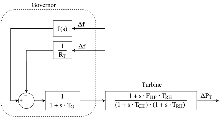
(a) Thermal power plant

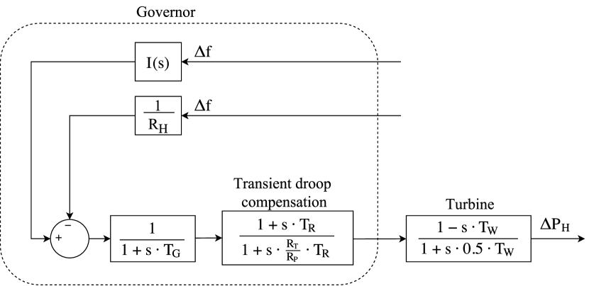
(b) Hydro-power plant

Figure 1: Conventional power plant models.

The power system model for frequency deviation analysis is based on the swing equation, see Section 2,

$$\Delta f=\dfrac{1}{2\;H_{eq}\;s+D_{eq}}\cdot(\Delta P_{g}-\Delta P_{load}),$$ (4)

where $\Delta P_{g}=\Delta P_{RES}+\Delta P_{T}+\Delta P_{H}$ is the active power variation from supply-side and $\Delta P_{load}$ is the demand-side variation. $H_{eq}$ is the equivalent inertia of the power system according to eq. (3) and $D_{eq}$ is the damping factor, considered as constant $D_{eq}=2$ %/Hz following the ENTSO-E recommendations entsoe_frequency . The power imbalance $\Delta P_{L}$ is simulated as a sudden step. Most frequency deviation analysis only consider a reduced number of such sudden imbalances, as was discussed in Section 1. To overcome this drawback, $\Delta P_{L}$ varies from 2.5% to 40% (2.5% steps) following the ENTSO-E recommendations previously discussed in Section 2.2.

3.2 Virtual inertia and additional power estimation

Following the case studies explained in Section 3.1, the equivalent synchronous inertia of each simulated scenario is determined by eq. (2). This equivalent inertia lies between 8.71 s (5% RES, $H_{T}=10$ s and $H_{H}=4.75$ s) and 0.76 s (60% RES, $H_{T}=2$ s and $H_{H}=1.75$ s). Authors analyse such $H_{eq}$ variations to emphasise the relevance of such conventional power plant inertia constants. Indeed, small $H$ variations can drastically affect the whole inertia power system $H_{eq}$, and subsequently, the minimum additional virtual inertia to be provided by the other sources. As will be discussed in Section 4, only by considering the synchronous inertia, the ROCOF limits would be violated (especially for imbalances $\Delta P_{L}\geq 20$%) and the nadir frequency would be lower than 49.2 Hz in most cases. Consequently, the virtual additional inertia that should be provided $H_{RES}$ to fulfil the ROCOF limits established by ENTSO-E, as well as the additional power $\Delta P_{add}$ to be within the allowable dynamical variation of frequency, are estimated. Both virtual inertia and additional supply-side power can be provided by a variety of different, complementary solutions/resources, which can be combined in an optimised power system source environment.

3.2.1 Estimation of minimum $H_{RES}$

From the ROCOF limits presented in Section 2.2, the minimum system inertia can be obtained as

$$H_{eq,min}=\dfrac{\Delta P_{L}}{P_{load}}\cdot\dfrac{f_{0}}{ROCOF_{lim}},$$ (5)

where $\Delta P_{L}$ is the power imbalance, $P_{load}$ is the total load of the power system, $f_{0}$ is the nominal frequency and $ROCOF_{lim}$ is the maximum limit ROCOF allowed entsoe_frequency . Combining eqs. (3) and (5), it is possible to obtain the minimum $H_{RES}$ required to fulfil the ROCOF limits:

$$H_{RES}=\dfrac{H_{eq,min}\cdot S_{B}-H_{T}\cdot S_{B,T}-H_{H}\cdot S_{B,H}}{S_{B,RES}}.$$ (6)

In consequence, an algorithm to estimate the minimum RES inertia constant $H_{RES}$ is proposed, see Figure 2,

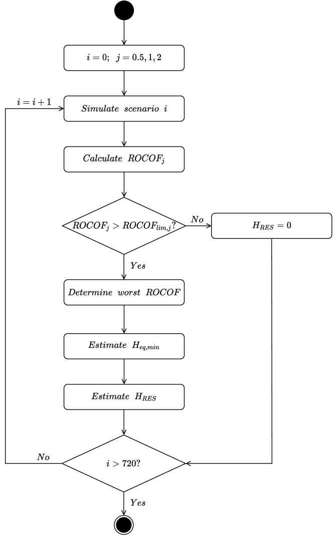
Figure 2: Graphic description to estimate minimum $H_{RES}$ according to the ENTSO-E recommendations.

1. Simulate the $i$–scenario, depending on the RES percentage, conventional generation units’ inertia ($H_{T}$ and $H_{H}$, respectively), and power imbalance $\Delta P_{L}$.

2. Determine each ROCOF_j (being $j=0.5$, $1$ and $2$) with eq. (7)–(9), where $t_{0}$ is the imbalance time instant (in $s$):

   $$ROCOF_{0.5}=\dfrac{\Delta f_{t_{0}+0.5}-\Delta f_{t_{0}}}{0.5},$$ (7)

   $$ROCOF_{1}=\dfrac{\Delta f_{t_{0}+1}-\Delta f_{t_{0}}}{1},$$ (8)

   $$ROCOF_{2}=\dfrac{\Delta f_{t_{0}+2}-\Delta f_{t_{0}}}{2}.$$ (9)

3. Check whether any of the previously determined ROCOF_j is over their limit: ROCOF${}_{0.5}>2$ Hz/s, ROCOF${}_{1}>1.5$ Hz/s, and/or ROCOF${}_{2}>1.25$ Hz/s.

   1. If no ROCOF_j exceeds the corresponding limit, non-additional inertia is required ($H_{RES}=0$), and the following scenario is then simulated ($i=i+1$).

   2. If one (or more) of the ROCOF_j exceed/s its/their limits, the algorithm proceeds to the next step.

4. Determine the worst ROCOF_j value. This is performed by calculating the relative differences between each ROCOF_j exceeding the limits and the corresponding ROCOF_lim,j (in %). The maximum value of such relative differences is then considered for the next step.

5. Estimate the minimum equivalent inertia $H_{eq,min}$ (eq. (5)) for the worst ROCOF previously determined, considering ROCOF_lim as 2, 1.5 or 1.25 Hz/s depending on ROCOF_j (0.5, 1 or 2), respectively.

6. Calculate the additional RES inertia constant $H_{RES}$ from eq. (6).

7. Simulate the following ($i=i+1$) scenario, finishing the algorithm when all scenarios under consideration are simulated ($i>720$).

3.2.2 Estimation of minimum $\Delta P_{add}$

According to ENTSO-E, the maximum dynamic variation of frequency is $f_{0}\pm 800$ mHz. Moreover, if $f\leq 47.5$ Hz, it is difficult to avoid a power system blackout entsoe_frequency . These frequency limits are exceeded in most of the supply-side scenarios currently under analysis. Consequently, some additional power $\Delta P_{add}$ should be provided to be within the dynamic range of such frequency variations. The estimated $\Delta P_{add}$ can be provided by: $(i)$ additional power from RES (by including frequency control strategies), $(ii)$ energy storage solutions, $(iii)$ increasing the PFR of conventional power plants, $(iv)$ other power systems from interconnections, or $(v)$ a combination of them. Taking into account the power system discussed in Section 3.1, the corresponding additional active power $\Delta P_{add}$ is then estimated as follows, see Figure 3:

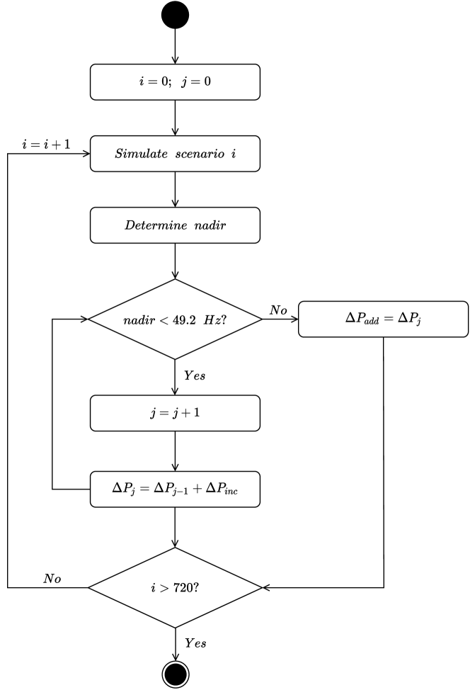
Figure 3: Graphic description to estimate minimum $\Delta P_{add}$ according to the ENTSO-E recommendations.

1. Simulate the $i$–scenario, which depends on the RES integration, conventional generation units’ inertia ($H_{T}$ and $H_{H}$, respectively) and power imbalance $\Delta P_{L}$.

2. Determine the nadir (minimum value of the frequency deviation).

3. Check if the nadir value is below 49.2 Hz (800 mHz deviation) as recommended by ENTSO-E.

   1. If nadir is $f\geq 49.2$ Hz, no additional power is needed ($\Delta P_{add}=0$), and a new scenario is simulated ($i=i+1$), going back to the first step of the algorithm.

   2. If nadir is below 49.2 Hz, the algorithm proceeds to the next step.

4. Increase the additional power $\Delta P_{j}$ by a predefined value $\Delta P_{inc}$. In this case, $\Delta P_{inc}=0.01$ pu. This step is repeated until the nadir value is over 49.2 Hz.

5. Simulate the following ($i=i+1$) scenario, finishing the algorithm when all scenarios under consideration are simulated ($i>720$).

4 Results

4.1 Case study discussion

Considering the recommendations of ENTSO-E previously discussed in Section 2.2 as well as current RES integration and roadmaps cited in Section 3.1, 5 different RES integration levels and 16 different power imbalances are identified for simulation and analysis purposes. Although the existing studies offer no guidance for the maximum RES limit integration, the percentage to maintain the system frequency response within the permissible bounds is estimated to be around 50% 8106748 , or even higher by other authors with the installation of small, but highly efficient storage devices weitemeyer15 . Hydro-power capacity remains constant in all cases. Thermal capacity decreases proportionately as RES capacity increases. The five generation mix cases are summarised in Table 1. These generation mix cases are in line with those proposed by the 10-year network development plan for the EU tyndp2020scenarios . The power imbalance $\Delta P_{L}$ increases from 2.5% up to 40% in 2.5% steps.

Table 1: Generation by source

Supply-side resource	Mix generation (%)
Thermal power plant	80	70	55	40	25
Hydro-power plant	15	15	15	15	15
Renewable power plant	5	15	30	45	60

Most of previous contributions discussed in Section 1 assume a supply-side modelling without any parameter diversity in their equivalent generation units. Following the recent review by fernandez19 , three different values for the inertia constant of the thermal $H_{T}$ and hydro-power $H_{H}$ plants are considered for simulations. The minimum, mean and maximum value of such inertia constants are then taken into account: $H_{T}=\left\{2,6,10\right\}$, $H_{H}=\left\{1.75,3.25,4.75\right\}$. Therefore, by combining the different $\Delta P_{L}$ (16), RES integration (5), $H_{T}$ (3) and $H_{H}$ (3), 720 scenarios are identified and simulated. The equivalent synchronous inertia corresponding to the conventional generation units (i.e., thermal and hydro-power) is then determined from eq. (2), which also depends on the RES integration. All of the simulations are carried out under a Matlab/Simulink environment.

4.2 Results

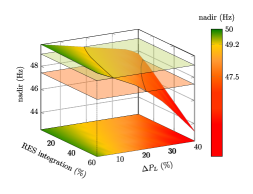
(a) Nadir frequency

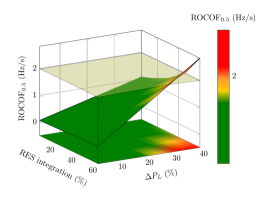
(b) ROCOF_0.5 overview

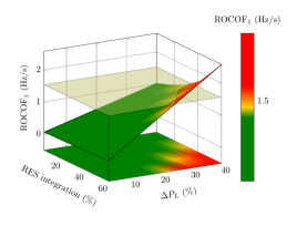
(c) ROCOF₁ overview

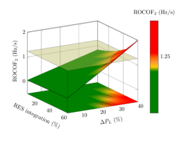
(d) ROCOF₂ overview

Figure 4: Overview of nadir frequency and ROCOFs when $H_{T}=10$ s and $H_{H}=4.75$ s

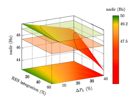
(a) Nadir frequency

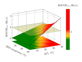
(b) ROCOF_0.5 overview

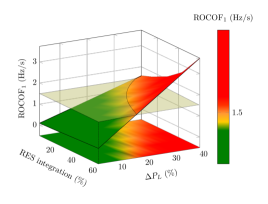
(c) ROCOF₁ overview

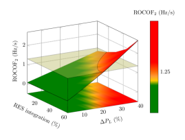
(d) ROCOF₂ overview

Figure 5: Overview of nadir frequency and ROCOFs when $H_{T}=6$ s and $H_{H}=3.25$ s

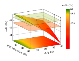
(a) Nadir frequency

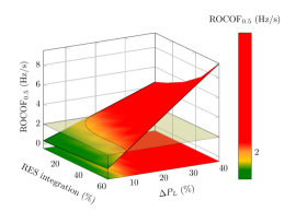
(b) ROCOF_0.5 overview

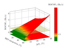
(c) ROCOF₁ overview

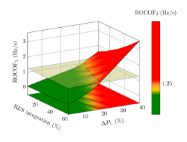
(d) ROCOF₂ overview

Figure 6: Overview of nadir frequency and ROCOFs when $H_{T}=6$ s and $H_{H}=3.25$ s

Figures 4–6 depict 240 cases out of the 720 under consideration. In each figure, 80 scenarios are summarised (combination of the 16 power imbalances and the 5 generation mix). Both the nadir frequency and the three ROCOF values for three different combinations of $H_{T}$ and $H_{H}$ are depicted, being significant the diversity of results under a variety of such parameters, commonly assumed as constant in most of previous contributions as was discussed in Section 1. The equivalent synchronous inertia of the system for each figure is detailed in Table 4.2, depending on the RES integration.

Synchronous equivalent inertia ($H_{eq}$). Example of results RES Integration (%) 5 15 30 45 60 $H_{T}=10$ 8.71 7.71 6.21 4.71 3.21 $H_{H}=4.75$ $H_{T}=6$ 5.29 4.69 3.79 2.89 1.99 $H_{H}=3.25$ $H_{T}=2$ 1.86 1.66 1.36 1.06 0.76 $H_{H}=1.75$

With regard to nadir frequency, values over $f\geq 49.2$ Hz are dynamically accepted by ENTSO-E. As a consequence, they are coloured in green. If the nadir decreases under $f<49.2$ Hz (but is still over $f\geq 47.5$ Hz), it is coloured in yellow and orange, as they are outside the dynamic range allowed by ENTSO-E. When nadir is under $f<47.5$ Hz, a possible blackout may occur in the grid, subsequently being coloured in red. Two different planes are included in Figures 4–6 determining such limits. As can be seen, most of the scenarios under consideration are outside the dynamically accepted range, especially if both the RES integration and the power imbalance are high. Even though the equivalent synchronous inertia is significantly reduced depending on the $H_{T}$ and $H_{H}$ values (for instance, $H_{eq}=8.71$ s, $H_{eq}=5.29$ s or $H_{eq}=1.86$ s for 5% RES integration, refer to Table 4.2), the nadir frequency does not decrease drastically for the same generation mix. In fact, if comparing the 5% RES integration energy mix, and the imbalance $\Delta P_{L}=2.5$%, the nadir frequencies are 49.88, 49.86 and 49.80 Hz, from the highest to the lowest combination values of $H_{T}$ and $H_{H}$. Similar results are obtained for the worst scenario (i.e., 60% RES integration energy mix and the imbalance $\Delta P_{L}=40$%), where the nadir frequencies are 43.33, 43.33 and 42.75 Hz, respectively.

By considering the three ROCOF values, the limits established by ENTSO-E are ROCOF${}_{0.5}\leq 2$ Hz/s, ROCOF${}_{1}\leq 1.5$ Hz/s and ROCOF${}_{2}\leq 1.25$ Hz/s for the 0.5, 1 and 2 s time-window, respectively. ROCOF values are coloured in accordance to their limits, in line with the nadir frequency.Most scenarios under consideration are outside the limits determined, especially if both the RES integration and the power imbalance $\Delta P_{L}$ are high values. In contrast to nadir values, ROCOFs are really dependent on the synchronous equivalent inertia. Indeed, the lower the $H_{eq}$, the higher the ROCOFs values (compare, for instance, the ROCOFs of Figure 4 to those values of Figure 6).

4.3 $H_{RES}$ and $\Delta P_{add}$ estimation

(a) $\Delta P_{add}$ to fulfil nadir frequency limit

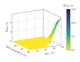
(b) $H_{RES}$ to fulfil ROCOFs limits

Figure 7: $H_{RES}$ and $\Delta P_{add}$ estimation ($H_{T}=10$ s, $H_{H}=4.75$ s).

(a) $\Delta P_{add}$ to fulfil nadir frequency limit

(b) $H_{RES}$ to fulfil ROCOFs limits

Figure 8: $H_{RES}$ and $\Delta P_{add}$ estimation ($H_{T}=6$ s, $H_{H}=3.25$ s).

Following the methodology described in Section 3.2, the virtual inertia $H_{RES}$ to fulfil the ROCOF limits, and the additional active power $\Delta P_{add}$ needed to be within the dynamic range of frequency variations are estimated. The results shown in Figures 7–9 correspond to the 240 cases presented in Figures 4–6.

(a) $\Delta P_{add}$ to fulfil nadir frequency limit

(b) $H_{RES}$ to fulfil ROCOFs limits

Figure 9: $H_{RES}$ and $\Delta P_{add}$ estimation ($H_{T}=2$ s, $H_{H}=1.75$ s).

The additional power $\Delta P_{add}$ to be provided in order to avoid the nadir frequency under $f<49.2$ Hz takes a maximum value of 0.32 pu. This $\Delta P_{add}$ can be given by different resources (such as including RES in frequency control, storage solutions, increasing the PFR of conventional power plants, interconnections, or a combination of some of these). As can be seen in Figures 7–9, the higher the RES integration and $\Delta P_{L}$, the higher the additional power $\Delta P_{add}$ required. In fact, a lineal regression with $R^{2}=0.96$ depending on the RES integration and the $\Delta P_{L}$ can be deduced.

With regard to $H_{RES}$, some of the estimated results may lead to unrealistic solutions. Indeed, a maximum value of $H_{RES}=96$ s was obtained. This $H_{RES}$ could also come from different resources. Moreover, the RES virtual inertia constant does not have any physical meaning (and an arbitrary value could be set). According to zhang12 ; krpan2017inertial , the most appropriate value for VSWT is $1.85\cdot H_{WT}$ (being $H_{WT}$ the inertia constant of the wind turbine) to avoid the stalling of the turbine. As a result, a maximum $H_{RES}$ of 15 s is considered in Figures 7–9, which is slightly over inertia constants of conventional power plants (2–10 s) fernandez19 ; fernandez19analysis . By considering this maximum limit, ROCOF is within the limits of the ENTSO-E recommendations for 85% of the analysed cases (612 scenarios).

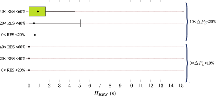
(a) Thermal and hydro inertia constant scenarios for 0<$\Delta P_{L}$<20.

(b) Thermal and hydro inertia constant scenarios for 20<$\Delta P_{L}$<40.

Figure 10: $H_{RES}$ to fulfil ROCOFs limits: summary of virtual inertia values.

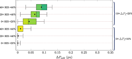
(a) Thermal and hydro inertia constant scenarios for 0<$\Delta P_{L}$<20.

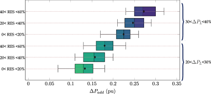
(b) Thermal and hydro inertia constant scenarios for 20<$\Delta P_{L}$<40.

Figure 11: $\Delta P_{add}$ to fulfil nadir frequency limit: summary of values.

4.4 Discussion

The recommended inertia constant of future power systems, according to ENTSO-E, ranges in between 2–3 s entsoe_high , whereas in conventional power plants it used to be 5–6 s entsoe_si . In this study, authors have considered cases in which $H_{eq}$ is lower and higher than such recommended values, corresponding to a wide range of RES. In fact, under the same RES integration percentage, a relevant variety of $H_{eq}$ is obtained, highly depending on the $H_{T}$ and $H_{H}$, refer to Table 4.2. As a result, the different values of $H$ for conventional power plants is identified as a major importance to properly carry out frequency deviation studies for future scenarios.

As was mentioned in Section 1, PV and wind resources are considered as the most promising RES technologies. The absence of rotational parts in PV power plants implies an inertia constant $H\approx 0$ tielens17phd . The stored kinetic energy and, subsequently, deployable inertia of VSWTs is not directly available due to the power inverter gonzalez2014frequency . As a consequence, the more the RES penetration into a power system, the weaker it will be in terms of frequency stability due to the reduction of $H_{eq}$ pulgar2017inertia ; fang2018improved . Consequently, the maximum penetration of RES for this $H_{eq,min}$ of 2–3 s is between 50-70%. In fact, some authors affirm that with current RES technologies, only 50% of the overall electricity demand can be provided by them zakeri15 ; weitemeyer15 . This RES integration discussion should also include an extensive frequency response analysis, which is the aim of this work. The 720 scenarios previously analysed have been then simulated by including the results of $H_{RES}$ and $\Delta P_{add}$ estimated in Section 4.3. In this way, it is then possible to verify that $H_{RES}$ and $\Delta P_{add}$ values are suitable to fulfil the ENTSO-E recommendations. Figure 10 summarises in a box-and-whisker plot the virtual inertia values for all thermal and hydro inertia constant scenarios depending on the RES integration and the power imbalance. A maximum 15 s for virtual inertia is assumed by the authors to achieve such requirements. Additionally, Figure 11 depicts the corresponding $\Delta P_{add}$ values in a box-and-whisker plot.

Finally, and as examples of these frequency excursion analysis, some scenarios are depicted in Figures 12–13, including the frequency evolution and the three ROCOF values considering in the ENTSO-E requirements. Different inertia values for $H_{T}$ and $H_{H}$, together with several imbalances $\Delta P_{L}$ and RES integration levels are shown. As can be seen, all nadirs are $f\geq 49.2$ Hz, thus staying in the dynamic accepted range of frequency variations. Moreover, the three ROCOF values are lower than their recommended limit values. As a consequence, the proposed methodology is suitable to estimate $\Delta P_{add}$ and $H_{RES}$ values, and it can be apply to other international power system requirements.

(a) Frequency evolution for $\Delta P_{L}=20$%

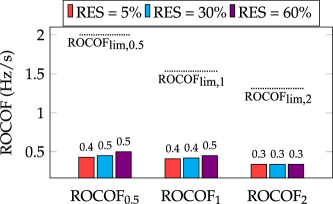
(b) ROCOF values for $\Delta P_{L}=20$%

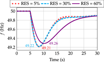
(c) $\Delta P_{L}=40$%

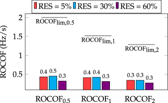
(d) ROCOF values for $\Delta P_{L}=40$%

Figure 12: Frequency evolution and ROCOF values ($H_{T}=10$ s, $H_{H}=4.75$ s).

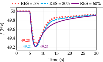
(a) Frequency evolution for $\Delta P_{L}=12.5$%

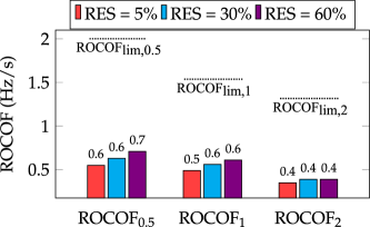
(b) ROCOF values for $\Delta P_{L}=12.5$%

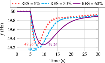
(c) $\Delta P_{L}=35$%

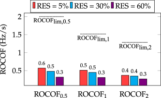
(d) ROCOF values for $\Delta P_{L}=35$%

Figure 13: Frequency evolution and ROCOF values ($H_{T}=6$ s, $H_{H}=3.25$ s).

5 Conclusion

This paper presents a detailed analysis of nadir and ROCOFs values following ENTSO-E recommendations for the interconnected European power system. A total of 720 generation mix scenarios are simulated, considering different RES integration (between 5% and 60%), power imbalance and inertia constants of conventional power plants (thermal and hydro-power). The minimum additional power and virtual inertia required to fulfil the nadir and ROCOF limits established by ENTSO-E are estimated for each scenario. The results show that an additional power between 0 and 0.32 pu is enough to avoid any frequency excursion lower than 49.2 Hz, even if RES generation is over 50% and the power imbalance is 40%. This additional power can be provided by a sort of sources, such as RES (through frequency control techniques), increasing the primary frequency reserves of conventional power plants, storage systems, provided by a different power system through interconnections, or a combination of some of them. Authors assume a maximum virtual inertia lower than 15 s. Under this assumption, the ROCOF values following the ENTSO-E requirements are fulfilled for 85% of the simulated scenarios. From our analysis, it can be deduced that the additional power and virtual inertia to support frequency deviations after power imbalances can be provided independently and from different resources. This is due to the fact that ROCOF is directly related to inertia, but nadir is not so affected by such parameter. This analysis is carried out considering the interconnected European power system. Nevertheless, it can be applied to any other power system with high penetration of renewable sources, considering the specific recommendations of such grid.

6 Acknowledgements

This work is supported by the Spanish Ministry of Education, Culture and Sport —FPU16/04282— and by the Spanish Ministry of Economy and Competitiveness and the European Union —FEDER Funds, ENE2016-78214-C2-1-R—.

References

- [1] D’hulst, R., Fernandez, J.M., Rikos, E., Kolodziej, D., Heussen, K., Geibelk, D., et al. ‘Voltage and frequency control for future power systems: the electra irp proposal’. In: Smart Electric Distribution Systems and Technologies (EDST), 2015 International Symposium on. (IEEE, 2015. pp. 245–250
- [2] Hadjipaschalis, I., Poullikkas, A., Efthimiou, V.: ‘Overview of current and future energy storage technologies for electric power applications’, Renewable and sustainable energy reviews, 2009, 13, (6-7), pp. 1513–1522
- [3] Zervos, A., Lins, C., Muth, J.: ‘RE-thinking 2050: a 100% renewable energy vision for the European Union’. (Erec, 2010)
- [4] Liu, G., Tomsovic, K.: ‘Quantifying spinning reserve in systems with significant wind power penetration’, IEEE Transactions on Power Systems, 2012, 27, (4), pp. 2385–2393
- [5] Huber, M., Dimkova, D., Hamacher, T.: ‘Integration of wind and solar power in europe: Assessment of flexibility requirements’, Energy, 2014, 69, (Supplement C), pp. 236 – 246
- [6] Tselepis, S., Nikoletatos, J.: ‘Renewable energy integration in power grids’, , 2015,
- [7] ‘The european power sector in 2017. state of affairs and review of current developments’. (Agora Energiewende and Sandbag, 2018.
- [8] Europe, W.: ‘Wind energy in europe: Scenarios for 2030’, Wind Europe: Brussels, Belgium, 2017,
- [9] Energy, S.P.: ‘Technology roadmap’, , 2014,
- [10] Zakeri, B., Syri, S., Rinne, S.: ‘Higher renewable energy integration into the existing energy system of finland–is there any maximum limit?’, Energy, 2015, 92, pp. 244–259
- [11] Ochoa.Correa, D., Martinez, S.: ‘Fast-frequency response provided by dfig-wind turbines and its impact on the grid’, IEEE Transactions on Power Systems, 2017, 32, pp. 4002–4011
- [12] Shah, R., Mithulananthan, N., Bansal, R.C., Ramachandaramurthy, V.K.: ‘A review of key power system stability challenges for large-scale PV integration’, Renewable and Sustainable Energy Reviews, 2015, 41, pp. 1423 – 1436
- [13] Green, R., Vasilakos, N.: ‘Market behaviour with large amounts of intermittent generation’, Energy Policy, 2010, 38, (7), pp. 3211–3220
- [14] Rodriguez, R.A., Becker, S., Andresen, G.B., Heide, D., Greiner, M.: ‘Transmission needs across a fully renewable european power system’, Renewable Energy, 2014, 63, pp. 467–476
- [15] Zhang, W., Fang, K.: ‘Controlling active power of wind farms to participate in load frequency control of power systems’, IET Generation, Transmission & Distribution, 2017, 11, pp. 2194–2203(9)
- [16] Tielens, P., Van.Hertem, D.: ‘Grid inertia and frequency control in power systems with high penetration of renewables’, , 2012,
- [17] Spahic, E., Varma, D., Beck, G., Kuhn, G., Hild, V. ‘Impact of reduced system inertia on stable power system operation and an overview of possible solutions’. In: Power and Energy Society General Meeting (PESGM), 2016. (IEEE, 2016. pp. 1–5
- [18] Gautam, D., Goel, L., Ayyanar, R., Vittal, V., Harbour, T.: ‘Control strategy to mitigate the impact of reduced inertia due to doubly fed induction generators on large power systems’, IEEE Transactions on Power Systems, 2011, 26, (1), pp. 214–224
- [19] Delille, G., Francois, B., Malarange, G.: ‘Dynamic frequency control support by energy storage to reduce the impact of wind and solar generation on isolated power system’s inertia’, IEEE Transactions on Sustainable Energy, 2012, 3, (4), pp. 931–939
- [20] Daly, P., Flynn, D., Cunniffe, N. ‘Inertia considerations within unit commitment and economic dispatch for systems with high non-synchronous penetrations’. In: PowerTech, 2015 IEEE Eindhoven. (IEEE, 2015. pp. 1–6
- [21] Du, P., Matevosyan, J.: ‘Forecast system inertia condition and its impact to integrate more renewables’, IEEE Transactions on Smart Grid, 2018, 9, (2), pp. 1531–1533
- [22] Xu, T., Liu, Y., Overbye, T.J. ‘Metric development for evaluating inertia’s locational impacts on system primary frequency response’. In: Texas Power and Energy Conference (TPEC), 2018 IEEE. (IEEE, 2018. pp. 1–6
- [23] Negnevitsky, M., Nguyen, D.H., Piekutowski, M.: ‘Risk assessment for power system operation planning with high wind power penetration’, IEEE Transactions on Power Systems, 2015, 30, (3), pp. 1359–1368
- [24] Fu, Y., Wang, Y., Zhang, X.: ‘Integrated wind turbine controller with virtual inertia and primary frequency responses for grid dynamic frequency support’, IET Renewable Power Generation, 2017, 11, (8), pp. 1129–1137
- [25] Nguyen, H.T., Yang, G., Nielsen, A.H., Jensen, P.H. ‘Frequency stability improvement of low inertia systems using synchronous condensers’. In: 2016 IEEE International Conference on Smart Grid Communications (SmartGridComm). (, 2016. pp. 650–655
- [26] Kerdphol, T., Rahman, F.S., Mitani, Y.: ‘Virtual inertia control application to enhance frequency stability of interconnected power systems with high renewable energy penetration’, Energies, 2018, 11, (4)
- [27] Canevese, S., Iaria, A., Rapizza, M. ‘Impact of fast primary regulation and synthetic inertia on grid frequency control’. In: 2017 IEEE PES Innovative Smart Grid Technologies Conference Europe (ISGT–Europe). (, 2017. pp. 1–6
- [28] Attya, A.B.T., Hartkopf, T.: ‘Control and quantification of kinetic energy released by wind farms during power system frequency drops’, IET Renewable Power Generation, 2013, 7, (3), pp. 210–224
- [29] Fernández.Guillamón, A., Sarasúa, J.I., Chazarra, M., Vigueras.Rodríguez, A., Fernández.Muñoz, D., Molina.García, Á.: ‘Frequency control analysis based on unit commitment schemes with high wind power integration: A spanish isolated power system case study’, International Journal of Electrical Power & Energy Systems, 2020, 121, pp. 106044
- [30] Wang, Y., Silva, V., Lopez-Botet-Zulueta, M.: ‘Impact of high penetration of variable renewable generation on frequency dynamics in the continental europe interconnected system’, IET Renewable Power Generation, 2016, 10, (1), pp. 10–16
- [31] Mosca, C., Arrigo, F., Mazza, A., Bompard, E., Carpaneto, E., Chicco, G., et al.: ‘Mitigation of frequency stability issues in low inertia power systems using synchronous compensators and battery energy storage systems’, IET Generation, Transmission Distribution, 2019, 13, (17), pp. 3951–3959
- [32] Bueno, P.G., Hernández, J.C., Ruiz-Rodriguez, F.J.: ‘Stability assessment for transmission systems with large utility-scale photovoltaic units’, IET Renewable Power Generation, 2016, 10, (5), pp. 584–597
- [33] Pschel.LØvengreen, S., Mancarella, P. ‘Frequency response constrained economic dispatch with consideration of generation contingency size’. In: 2018 Power Systems Computation Conference (PSCC). (IEEE, 2018. pp. 1–7
- [34] Fenández.Guillamón, A., Molina.Garcia, A., Vigueras.Rodríguez, A., Gómez.Lázaro, E. ‘Frequency response and inertia analysis in power systems with high wind energy integration’. In: International Conference on Clean Electrical Power – ICCEP, Italy. (IEEE, 2019. pp. 1–6
- [35] Boldea, I.: ‘Synchronous generators’. (CRC Press, 2015)
- [36] Tielens, P., Van.Hertem, D.: ‘The relevance of inertia in power systems’, Renewable and Sustainable Energy Reviews, 2016, 55, pp. 999–1009
- [37] Fernández.Guillamón, A., Vigueras.Rodríguez, A., Molina.García, A. ‘Análisis y simulación de estrategias agregadas de control de frecuencia entre grandes parques eólicos y aprovechamientos hidroeléctricos’ [M.S. thesis]. Universidad Politécnica de Cartagena, 2017
- [38] Chiodo, E., Lauria, D., Mottola, F. ‘On-line bayes estimation of rotational inertia for power systems with high penetration of renewables. part i: Theoretical methodology’. In: 2018 International Symposium on Power Electronics, Electrical Drives, Automation and Motion (SPEEDAM). (IEEE, 2018. pp. 835–840
- [39] Li, W., Du, P., Lu, N.: ‘Design of a new primary frequency control market for hosting frequency response reserve offers from both generators and loads’, IEEE Transactions on Smart Grid, 2017,
- [40] Nedd, M., Booth, C., Bell, K. ‘Potential solutions to the challenges of low inertia power systems with a case study concerning synchronous condensers’. In: Universities Power Engineering Conference (UPEC), 2017 52nd International. (IEEE, 2017. pp. 1–6
- [41] Ulbig, A., Borsche, T.S., Andersson, G.: ‘Analyzing rotational inertia, grid topology and their role for power system stability’, IFAC-PapersOnLine, 2015, 48, (30), pp. 541–547
- [42] Aho, J., Buckspan, A., Laks, J., Fleming, P., Jeong, Y., Dunne, F., et al. ‘A tutorial of wind turbine control for supporting grid frequency through active power control’. In: 2012 American Control Conference (ACC). (, 2012. pp. 3120–3131
- [43] Kayikçi, M., Milanovic, J.V.: ‘Dynamic contribution of dfig-based wind plants to system frequency disturbances’, IEEE Transactions on Power Systems, 2009, 24, (2), pp. 859–867
- [44] Toulabi, M., Bahrami, S., Ranjbar, A.M.: ‘An input-to-state stability approach to inertial frequency response analysis of doubly-fed induction generator-based wind turbines’, IEEE Transactions on Energy Conversion, 2017, 32, (4), pp. 1418–1431
- [45] Sun, Y.z., Zhang, Z.s., Li, G.j., Lin, J. ‘Review on frequency control of power systems with wind power penetration’. In: Power System Technology (POWERCON), 2010 International Conference on. (IEEE, 2010. pp. 1–8
- [46] Dreidy, M., Mokhlis, H., Mekhilef, S.: ‘Inertia response and frequency control techniques for renewable energy sources: A review’, Renewable and Sustainable Energy Reviews, 2017, 69, pp. 144–155
- [47] Fernández.Guillamón, A., Gómez.Lázaro, E., Muljadi, E., Molina.García, Á.: ‘Power systems with high renewable energy sources: A review of inertia and frequency control strategies over time’, Renewable and Sustainable Energy Reviews, 2019, 115, pp. 109369
- [48] Morren, J.. ‘PhD Grid support by power electronic converters of distributed generation units (TU Delft)’. (, 2006
- [49] Tielens, P., Van.Hertem, D.: ‘Receding horizon control of wind power to provide frequency regulation’, IEEE Transactions on Power Systems, 2017, 32, (4), pp. 2663–2672
- [50] Fernández.Guillamón, A., Vigueras.Rodríguez, A., Molina.García, Á.: ‘Analysis of power system inertia estimation in high wind power plant integration scenarios’, IET Renewable Power Generation, 2019, 13, (15), pp. 2807–2816
- [51] ENTSO-E. ‘Electricity balancing in Europe’. (, . Available from: https://docstore.entsoe.eu/
- [52] ENTSO-E. ‘High Penetration of Power Electronic Interfaced Power Sources (HPoPEIPS)’. (, . Available from: https://consultations.entsoe.eu/
- [53] ENTSO-E. ‘Need for synthetic inertia (SI) for frequency regulation’. (, 2017.11. Available from: https://consultations.entsoe.eu/
- [54] ENTSO-E. ‘Rate of Change of Frequency (RoCoF) withstand capability’. (, . Available from: https://docstore.entsoe.eu/
- [55] ENTSO-E. ‘Frequency Stability Evaluation Criteria for the Synchronous Zone of Continental Europe ’. (, . Available from: https://docstore.entsoe.eu/
- [56] ENTSO-E. ‘Explanatory note for the FCR dimensioning rules proposal’. (, . Available from: https://consultations.entsoe.eu/
- [57] ENTSO.E. ‘Nc load frequency control & reserve: Overview last developments’. (, 2012. Available from: https://www.entsoe.eu/
- [58] ENTSO-E. ‘Explanatory document for the Nordic synchronous area Proposal for the dimensioning rules for FCR in accordance with Article 153 of the Commission Regulation (EU) 2017/1485 of 2 August 2017 establishing a guideline on electricity transmission system operation’. (, . Available from: https://consultations.entsoe.eu/
- [59] Kundur, P., Balu, N.J., Lauby, M.G.: ‘Power system stability and control’. vol. 7. (McGraw-hill New York, 1994)
- [60] Ahmadyar, A.S., Riaz, S., Verbič, G., Chapman, A., Hill, D.J.: ‘A framework for assessing renewable integration limits with respect to frequency performance’, IEEE Transactions on Power Systems, 2018, 33, (4), pp. 4444–4453
- [61] Weitemeyer, S., Kleinhans, D., Vogt, T., Agert, C.: ‘Integration of renewable energy sources in future power systems: The role of storage’, Renewable Energy, 2015, 75, pp. 14 – 20
- [62] ENTSO-E: ‘Ten–Year Network Development Plan (TYNDP) 2020 – Scenario Report’, , 2020, Available from: https://tyndp.entsoe.eu/scenarios/
- [63] Zhang, Z.S., Sun, Y.Z., Lin, J., Li, G.J.: ‘Coordinated frequency regulation by doubly fed induction generator-based wind power plants’, IET Renewable Power Generation, 2012, 6, (1), pp. 38–47
- [64] Krpan, M., Kuzle, I.: ‘Inertial and primary frequency response model of variable-speed wind turbines’, The Journal of Engineering, 2017, 2017, (13), pp. 844–848
- [65] Tielens, P.. ‘PhD Operation and control of power systems with low synchronous inertia (KU Leuven)’. (, 2017. Available from: https://core.ac.uk/download/pdf/95687043.pdf
- [66] Gonzalez.Longatt, F. ‘Frequency control and inertial response schemes for the future power networks’. In: Large Scale Renewable Power Generation. (Springer, 2014. pp. 193–231
- [67] Pulgar.Painemal, H., Wang, Y., Silva.Saravia, H.: ‘On inertia distribution, inter-area oscillations and location of electronically-interfaced resources’, IEEE Transactions on Power Systems, 2017, 33, (1), pp. 995–1003
- [68] Fang, J., Lin, P., Li, H., Yang, Y., Tang, Y.: ‘An improved virtual inertia control for three-phase voltage source converters connected to a weak grid’, IEEE Transactions on Power Electronics, 2018, 34, (9), pp. 8660–8670