Dynamic wormhole geometries in hybrid metric-Palatini gravity

Abstract

In this work, we analyse the evolution of time-dependent traversable wormhole geometries in a Friedmann-Lemaître-Robertson-Walker background in the context of the scalar-tensor representation of hybrid metric-Palatini gravity. We deduce the energy-momentum profile of the matter threading the wormhole spacetime in terms of the background quantities, the scalar field, the scale factor and the shape function, and find specific wormhole solutions by considering a barotropic equation of state for the background matter. We find that particular cases satisfy the null and weak energy conditions for all times. In addition to the barotropic equation of state, we also explore a specific evolving wormhole spacetime, by imposing a traceless energy-momentum tensor for the matter threading the wormhole and find that this geometry also satisfies the null and weak energy conditions at all times.

I Introduction

The explanation of the accelerated expansion of the Universe is one of the most challenging problems in modern cosmology Perlmutter:1998np ; Riess:1998cb . From the mathematical point of view, the simplest way to treat this problem is to consider the cosmological constant term Carroll:2000fy . Nonetheless, this model faces some difficulties such as the coincidence problem and the cosmological constant problem. The latter dictates a huge discrepancy between the observed values of the vacuum energy density and the theoretical large value of the zero-point energy suggested by quantum field theory Carroll:2000fy . There are some alternative models proposed to overcome these problems such as modified gravity Nojiri:2010wj ; Sotiriou:2008rp ; Capozziello:2011et ; Avelino:2016lpj ; Lobo:2008sg ; Bamba:2015uma ; Nojiri:2017ncd , mysterious energy-momentum sources Copeland:2006wr ; Horndeski:1974wa ; Deffayet:2011gz , such as quintessence Wetterich:1987fm ; Ratra:1987rm ; Caldwell:1997ii ; Zlatev:1998tr and $k$-essence ArmendarizPicon:1999rj ; ArmendarizPicon:2000dh ; ArmendarizPicon:2000ah fields, and complex equations of state storing the missing energy of the dark side of the Universe Bento:2002ps ; Arun:2017uaw . In general, models with varying dark energy candidates may be capable of overcoming all the mathematical and theoretical difficulties, however, the main underlying question is the origin of these terms. One proposal is to relate this behavior to the energy of quantum fields in vacuum through the holographic principle which allows us to reconcile infrared (IR) and ultraviolet (UV) cutoffs Cohen:1998zx (see Ref. Tawfik:2019dda for a review on various attempts to model the dark side of the Universe).

However, an alternative to these dark energy models, as mentioned above, is modified gravity Nojiri:2010wj ; Sotiriou:2008rp ; Capozziello:2011et ; Avelino:2016lpj ; Lobo:2008sg ; Bamba:2015uma ; Nojiri:2017ncd . Here, one considers generalizations of the Hilbert-Einstein Lagrangian specific curvature invariants such as $R^{2}$, $R_{\mu\nu}R^{\mu\nu}$, $R_{\alpha\beta\mu\nu}R^{\alpha\beta\mu\nu}$, $\varepsilon^{\alpha\beta\mu\nu}R_{\alpha\beta\gamma\delta}R_{\mu\nu}^{\gamma\delta}$, etc. A popular theory that has attracted much attention is $f(R)$ gravity, where one may tackle the problem through several approaches, namely, the metric formalism Nojiri:2010wj ; Sotiriou:2008rp ; Capozziello:2011et ; Avelino:2016lpj ; Lobo:2008sg ; Bamba:2015uma ; Nojiri:2017ncd , which considers that the metric is the fundamental field, or the Palatini formalism Olmo:2011uz , where here one varies the action with respect to the metric and an independent connection. However, one may also consider a hybrid combination of these approaches that has recently been proposed, namely, the hybrid metric-Palatini gravitational theory Harko:2011nh , where the metric Einstein-Hilbert action is supplemented with a metric-affine (Palatini) correction term. The hybrid metric-Palatini theory has the ability to avoid several of the problematic issues that arise in the pure metric and Palatini formalisms. For instance, metric $f(R)$ gravity introduces an additional scalar degree of freedom, which must possess a low mass in order to be relevant for the large scale cosmic dynamics. However, the presence of such a low mass scalar field would influence the dynamics on smaller scales, such as at the level of the Solar System, and since these small scale effects remain undetected, one must resort to screening mechanisms Capozziello:2007eu ; Khoury:2003rn . Relative to the Palatini formalism, no additional degrees of freedom are introduced, as the scalar field is an algebraic function of the trace of the energy-momentum tensor. It has been shown that this fact entails serious consequences for the theory, leading to the presence of infinite tidal forces on the surface of massive astrophysical type objects Olmo:2011uz .

In this context, the hybrid metric-Palatini gravity theories were proposed initially in Harko:2011nh in order to circumvent the above shorcomings in the metric and Palatini formalisms of $f(R)$ gravity. One of the main advantages of the hybrid metric-Palatini theory is that in its scalar-tensor representation a long-range force is introduced that automatically passes the Solar System tests, and thus no contradiction between the theory and the local measurements arise. In a cosmological context, it has also been shown that hybrid metric-Palatini gravity may also explain the cosmological epochs Lima:2014aza ; Lima:2015nma (we refer the reader to Capozziello:2015lza ; Harko:2018ayt ; Harko:2020ibn for more details). In fact, hybrid metric-Palatini gravity has attracted much attention recently, and has a plethora of applications, namely, in the galactic context Capozziello:2012qt ; Capozziello:2013yha ; Capozziello:2013uya , in cosmology Capozziello:2012ny ; Carloni:2015bua ; Capozziello:2013wq ; Boehmer:2013oxa ; Lima:2014aza ; Lima:2015nma , in braneworlds Fu:2016szo ; Rosa:2020uli , black holes Bronnikov:2019ugl ; Chen:2020evr ; Rosa:2020uoi ; Bronnikov:2020vgg , stellar solutions Danila:2016lqx , cosmic strings Bronnikov:2020zob ; Harko:2020oxq , tests of binary pulsars Avdeev:2020jqo , and wormholes Rosa:2018jwp ; Capozziello:2012hr , amongst others.

Here, we explore the possibility that evolving wormhole geometries may be supported by hybrid metric-Palatini gravity. These compact objects, which are theoretical shortcuts in spacetime, have been shown to be threaded by an exotic fluid that violates the null energy condition (NEC), at least for the static case Morris:1988cz ; Morris:1988tu . However, it has been shown that evolving wormholes are able to satisfy the energy conditions in arbitrary but finite intervals of time Kar:1994tz ; Kar:1995ss , contrary to their static counterparts Visser:1995cc ; Lobo:2017oab . One way to study this subject is to embed a wormhole in a Friedmann–Lemaître–Robertson–Walker (FLRW) metric, which permits the geometry to evolve in a cosmological background Roman:1992xj ; Anchordoqui:1997du ; Arellano:2006ex ; Ebrahimi:2009ih ; Ebrahimi:2009rv ; Bordbar:2010zz ; Sajadi:2012zz ; Cataldo:2013sma ; Setare:2015iqa ; Bhattacharya:2015oma ; Ovgun:2018uin ; Zangeneh:2014noa ; Cataldo:2008pm ; Cataldo:2008ku ; Cataldo:2012pw ; Maeda:2009tk ; KordZangeneh:2020jio . Due to the somewhat problematic nature of the energy condition violations, an important issue is whether traversable wormholes can be constructed from normal matter throughout the spacetime, or at least partially. Different wormhole structures have been explored from this point of view Zangeneh:2014noa ; Mehdizadeh:2015jra ; Mehdizadeh:2015dta ; Zangeneh:2015jda ; KordZangeneh:2020jio ; Parsaei:2019utg . Indeed, it has been shown that in modified gravity, it is possible to impose that the matter threading the wormhole throat satisfies the energy conditions Capozziello:2013vna ; Capozziello:2014bqa , and it is the higher order curvature terms that support these nonstandard wormhole geometries Lobo:2007qi ; Lobo:2009ip ; Garcia:2010xb ; MontelongoGarcia:2010xd ; Harko:2013yb ; Korolev:2020ohi . Furthermore, different wormhole structures have been studied extensively in the context of alternative theories of gravity Antoniou:2019awm ; Tangphati:2019pxh ; Papantonopoulos:2019ugr ; Godani:2019kgy ; Banerjee:2020uyi ; Fayyaz:2020jzh ; Restuccia:2020wls ; Tangphati:2020mir ; Singh:2020rai ; Ibadov:2020btp ; Richarte:2009zz and also from different aspects Lazov:2017tjs ; Savelova:2019lye ; Bak:2019nnu ; Xu:2020wfm ; Jusufi:2020rpw ; Berry:2020tky ; Fallows:2020ugr ; Maldacena:2020sxe ; Lobo:2020kxn ; Parsaei:2020hke ; DeFalco:2020afv ; Moti:2020whf ; Wielgus:2020uqz .

In this paper, we study the evolution of traversable wormholes in a FLRW universe background in the scalar-tensor representation of hybrid metric-Palatini gravity. Furthermore, we explore the energy conditions for matter which threads these wormhole geometries. The paper is organized in the following manner: In Sec. II, we briefly present the action and field equations of hybrid metric-Palatini gravity, we consider the spacetime metric and explore a barotropic equation of state for the background fluid. In Sec. III, we analyse evolving traversable wormhole geometries for specific values of the barotropic equation of state parameter, as well as evolving wormholes with a traceless energy-momentum tensor (EMT), and study the energy conditions for the solutions obtained. Finally, in Sec. IV, we summary our results and conclude.

II Evolving wormholes in hybrid metric-Palatini gravity

II.1 Action and field equations

Here, we briefly present the hybrid metric-Palatini gravitational theory. The action is given by

$$S=\frac{1}{2\kappa^{2}}\int d^{4}x\sqrt{-g}\left[R+f(\mathcal{R})\right]+S_{m}\ ,$$ (1)

where $\kappa^{2}\equiv 8\pi G$, $R$ is the metric Ricci scalar, and the Palatini curvature is $\mathcal{R}\equiv g^{\mu\nu}\mathcal{R}_{\mu\nu}$, with the Palatini Ricci tensor, $\mathcal{R}_{\mu\nu}$, defined in terms of an independent connection, $\hat{\Gamma}^{\alpha}_{\mu\nu}$, given by

$$\mathcal{R}_{\mu\nu}\equiv\hat{\Gamma}^{\alpha}_{\mu\nu,\alpha}-\hat{\Gamma}^{\alpha}_{\mu\alpha,\nu}+\hat{\Gamma}^{\alpha}_{\alpha\lambda}\hat{\Gamma}^{\lambda}_{\mu\nu}-\hat{\Gamma}^{\alpha}_{\mu\lambda}\hat{\Gamma}^{\lambda}_{\alpha\nu}\,,$$ (2)

and $S_{m}$ is the matter action.

However, the scalar-tensor representation of hybrid metric-Palatini gravity provides a theoretical framework which is easier to handle from a computational point of view Harko:2011nh , where the equivalent action to (1) is provided by

$$S=\int\frac{d^{4}x\sqrt{-g}}{2\kappa^{2}}\left[(1+\phi)R+\frac{3}{2\phi}\partial_{\mu}\phi\partial^{\mu}\phi-V(\phi)\right]+S_{m}.$$ (3)

Note a similarity with the the action of the $w=-3/2$ Brans-Dicke theory version of the Palatini approach to $f(R)$ gravity. However, the hybrid theory exhibits an important and subtle difference appearing in the scalar field-curvature coupling, which in the $w=-3/2$ Brans-Dicke theory is of the form $\phi R$ Harko:2011nh .

By varying the action (3) with respect to the metric provides the following gravitational field equation

$$G_{\mu\nu}=\kappa^{2}\left(\frac{1}{1+\phi}T_{\mu\nu}+T_{\mu\nu}^{(\phi)}\right),$$ (4)

where $T_{\mu\nu}$ is the standard matter energy-momentum tensor, and

$$T_{\mu\nu}^{(\phi)} = \frac{1}{\kappa^{2}}\frac{1}{1+\phi}\Bigg{[}\nabla_{\mu}\nabla_{\nu}\phi-\frac{3}{2\phi}\nabla_{\mu}\phi\nabla_{\nu}\phi$$ (5)

$$\text{\hskip 21.33955pt}+\Bigg{(}\frac{3}{4\phi}\nabla_{\lambda}\phi\nabla^{\lambda}\phi-\square\phi-\frac{1}{2}V\Bigg{)}g_{\mu\nu}\Bigg{]},$$

is the energy-momentum tensor of the scalar field of the theory.

Varying the action with the scalar field yields the following second-order differential equation,

$$-\square\phi+\frac{1}{2\phi}\partial_{\mu}\phi\partial^{\mu}\phi+\frac{\phi[2V-(1+\phi)V_{\phi}]}{3}=\frac{\phi\kappa^{2}}{3}T\ .$$ (6)

The above equation shows that in hybrid metric-Palatini gravity the scalar field is dynamical. This represents an important and interesting difference with respect to the standard Palatini case Olmo:2011uz .

II.2 Spacetime metric

The metric of a time-dependent wormhole geometry is given by

$$ds^{2}=-e^{2\Phi\left(r\right)}dt^{2}+a^{2}\left(t\right)\left[\frac{dr^{2}}{1-b\left(r\right)/r}+r^{2}d\Omega^{2}\right],$$ (7)

where $\Phi\left(r\right)$ and $b\left(r\right)$, respectively, are the redshift and shape functions, which are $r$-dependent, and $a\left(t\right)$ is the time-dependent scale factor, and $d\Omega^{2}=d\theta^{2}+\sin^{2}\theta d\varphi^{2}$ is the linear element of the unit sphere.

To correspond to a wormhole solution, the shape function has the following restrictions Morris:1988cz : (i) $b(r_{0})=r_{0}$, where $r_{0}$ is the wormhole throat, corresponding to a minimum radial coordinate, (ii) $b(r)\leq r$, and (iii) the flaring-out condition given in the form $rb^{\prime}(r)-b\left(r\right)<0$. The latter condition is the fundamental ingredient in wormhole physics, as taking into account the Einstein field equation, one verifies that this flaring-out condition imposes the violation of the NEC. In fact, it violates all of the pointwise energy conditions Morris:1988cz ; Morris:1988tu ; Visser:1995cc ; Lobo:2017oab ; Lobo:2004wq . In order to avoid the presence of event horizons, so that the wormhole is traversable, one also imposes that the redshift function, $\Phi(r)$, be finite everywhere. However, throughout this work, we consider a zero redshift function, $\Phi=0$, which simplifies the calculations significantly.

II.3 Evolving embedding analysis

It is also interesting to explore how the time evolution of the scale factor affects the wormhole itself. To this effect, in the following analysis, we will follow closely the analysis outlined in Refs. Morris:1988cz ; Roman:1992xj ; KordZangeneh:2020jio , and analyse how the (effective) radius of the throat or length of the wormhole changes it time. As mentioned above, throughout this paper, we consider $\Phi=0$ for simplicity. Thus, in order to analyse the time-dependent dynamic wormhole geometry, we need to choose a specific $b(r)$ to provide a reasonable wormhole at $t=0$, which is assumed to be the onset of the evolution. Note that the radial proper length between any two points $A$ and $B$, through the wormhole, at any $t={\rm const}$ is given by $l(t)=\pm\,a(t)\int_{r_{A}}^{r_{B}}{(1-b/r)^{-1/2}}\,dr$, which is merely the initial radial proper separation multiplied by the scale factor.

Now, to analyse how the “wormhole” form of the metric is maintained throughout the evolution, we consider a $t={\rm const}$ and $\theta=\pi/2$ slice of the spacetime (7). Thus, the metric reduces to

$$ds^{2}=\frac{a^{2}(t)\,dr^{2}}{1-b(r)/r}+a^{2}(t)\,r^{2}\,d\varphi^{2}\,,$$ (8)

and is embedded in a flat 3-dimensional Euclidean space given by

$$ds^{2}=d{\bar{z}}^{2}+d{\bar{r}}^{2}+{\bar{r}}^{2}\,{d\varphi}^{2}\,.$$ (9)

Comparing the angular coefficients, yields

$$\bar{r} = {a(t)\,r}\big{|}_{t={\rm const}}\,,$$ (10)

$${d\bar{r}}^{2} = a^{2}(t)\,{dr}^{2}\big{|}_{t={\rm const}}\,.$$ (11)

Note, that when considering derivatives, these relations do not represent a “coordinate transformation”, but a “rescaling” of the radial coordinate $r$ along each $t={\rm constant}$ slice.

The “wormhole” form of the metric will be preserved, with respect to the ${\bar{z}},{\bar{r}},\varphi$ coordinates, if the embedded slice has the following metric

$$ds^{2}=\frac{d{\bar{r}}^{2}}{1-\bar{b}(\bar{r})/\bar{r}}+{\bar{r}}^{2}{d\varphi}^{2}\,,$$ (12)

and the shape functions $\bar{b}(\bar{r})$ has a minimum at a specific $\bar{b}(\bar{r}_{0})=\bar{r}_{0}$. Now, the embedded slice (8) can be readily rewritten in the form of Eq. (12) by using Eqs. (10) and (11), and the following relation

$$\bar{b}(\bar{r})=a(t)\,b(r).$$ (13)

Thus, the evolving wormhole will have the same overall shape and size and relative to the ${\bar{z}},{\bar{r}},\varphi$ coordinate system, as the initial wormhole had relative to the initial $z,r,\varphi$ embedding space coordinate system. In addition to this, using Eqs. (9) and (12), one deduces that

$${{d{\bar{z}}}\over{d{\bar{r}}}}=\pm\left({{\bar{r}}\over{\bar{b}(\bar{r})}}-1\right)^{-1/2}={{dz}\over{dr}}\,,$$ (14)

which implies

$$\bar{z}(\bar{r}) = \pm\int{{d\bar{r}}\over{(\bar{r}/{\bar{b}(\bar{r})}-1)^{1/2}}}$$ (15)

$$= \pm\,a(t)\,\int{\left(\frac{r-b}{b}\right)^{-1/2}}\,dr$$

$$= \pm\,a(t)\,z(r)\,.$$

Thus, the relation between the initial embedding space at $t=0$ and the embedding space at any time $t$ is, from Eqs. (11) and (15)

$$ds^{2}=d{\bar{z}}^{2}+d{\bar{r}}^{2}+{\bar{r}}^{2}\,{d\varphi}^{2}=a^{2}(t)\,[dz^{2}+dr^{2}+r^{2}{d\varphi}^{2}]\,.$$ (16)

The wormhole will always remain the same size, relative to the ${\bar{z}},{\bar{r}},\phi$ coordinate system, as the scaling of the embedding space compensates for the evolution of the wormhole. Nevertheless, the wormhole will change size relative to the initial $t=0$ embedding space.

We also note that the “flaring out condition” for the evolving wormhole is given by

$${{d\,^{2}{\bar{r}(\bar{z})}}\over{d{\bar{z}}^{2}}}>0\,,$$ (17)

at or near the throat, so that taking into account Eqs. (10), (11), (13), and (14), it follows that

$${{d\,^{2}{\bar{r}(\bar{z})}}\over{d{\bar{z}}^{2}}}=\frac{1}{a(t)}\,{{b-b^{\prime}r}\over{2b^{2}}}=\frac{1}{a(t)}\,{{d\,^{2}r(z)}\over{dz^{2}}}>0\,,$$ (18)

at or near the throat. Using Eqs. (10), (13), and

$${\bar{b}}^{\prime}(\bar{r})={{d\bar{b}}\over{d\bar{r}}}=b^{\prime}(r)={{db}\over{dr}}\,,$$ (19)

the right-hand side of Eq. (18), relative to the ${\bar{z}},{\bar{r}},\phi$ coordinate system, may be written as

$${{d\,^{2}{\bar{r}(\bar{z})}}\over{d{\bar{z}}^{2}}}=\left({{\bar{b}-{\bar{b}}^{\prime}\bar{r}}\over{2{\bar{b}}^{2}}}\right)>0\,,$$ (20)

at or near the throat. Thus, we have verified that the flaring out condition (20), using the barred coordinates, has the same form as for the static wormhole.

II.4 Gravitational field equations

We also consider an anisotropic matter energy-momentum tensor given by $T_{\nu}^{\mu}={\rm diag}(-\rho,-\tau,p,p)$, where $\rho$, $\tau$ and $p$ are the energy density, the radial tension (which is equivalent to a negative radial pressure) and the tangential pressure, respectively. Using the metric (7), the gravitational field equations (4) provide the following energy-momentum profile:

$$\rho(t,r)=\left(3H^{2}+\frac{b^{\prime}}{r^{2}a^{2}}\right)\left(1+\phi\right)+3\dot{\phi}H+\frac{3\dot{\phi}^{2}}{4\phi}-\frac{1}{2}V(\phi),~{}$$ (21)

$$\tau\left(t,r\right) = \left(H^{2}+2\frac{\ddot{a}}{a}+\frac{b}{r^{3}a^{2}}\right)\left(1+\phi\right)$$ (22)

$$+2\dot{\phi}H-\frac{3\dot{\phi}^{2}}{4\phi}+\ddot{\phi}-\frac{1}{2}V(\phi),$$

$$p\left(t,r\right) = \left(-H^{2}-2\frac{\ddot{a}}{a}-\frac{rb^{\prime}-b}{2r^{3}a^{2}}\right)\left(1+\phi\right)$$ (23)

$$-2\dot{\phi}H+\frac{3\dot{\phi}^{2}}{4\phi}-\ddot{\phi}+\frac{1}{2}V(\phi),$$

respectively, where $H=\dot{a}/a$ and $\phi=\phi\left(t\right)$, the overdot and prime denote derivatives with respect to $t$ and $r$, respectively, and for notational simplicity, we have considered $\kappa=1$. One recovers the standard field equations of the Morris-Thorne wormhole Morris:1988cz , by fixing the scale factor $a$ to unity and excluding the background time-dependent evolution and the scalar field $\phi$ contribution.

Furthermore, we will also analyse the null and weak energy conditions for the solutions obtained below. The weak energy condition (WEC) is defined as $T_{\mu\nu}u^{\mu}u^{\nu}\geq 0$, where $u^{\mu}$ is a timelike vector, and is expressed in terms of the energy density $\rho$, radial tension $\tau$ and tangential pressure $p$ as $\rho\geq 0$, $\rho-\tau\geq 0$ and $\rho+p\geq 0$, respectively. The last two inequalities, i.e., $\rho-\tau\geq 0$ and $\rho+p\geq 0$ correspond to the NEC, which is defined as $T_{\mu\nu}k^{\mu}k^{\nu}\geq 0$, where $k^{\mu}$ is any null vector.

The scalar field equation of motion (6) yields

$$\ddot{\phi}+3\dot{\phi}H-\frac{\dot{\phi}^{2}}{2\phi}-\frac{1}{3}\phi\left[T+\left(1+\phi\right)\frac{dV}{d\phi}-2V(\phi)\right]=0,$$ (24)

where the trace of the energy-momentum tensor $T=T\left(t,r\right)=T_{\mu}^{\mu}=-\rho-\tau+2p$ is given by

$$T\left(t,r\right)=-2\left(\frac{b^{\prime}}{a^{2}r^{2}}+3H^{2}+3\frac{\ddot{a}}{a}\right)(1+\phi)$$

$$-3\ddot{\phi}+\frac{3\dot{\phi}^{2}}{2\phi}-9\dot{\phi}H+2V(\phi).$$ (25)

In order to solve the differential equation (24) for $\phi\left(t\right)$, the trace $T\left(t,r\right)$, given by Eq. (25), should be independent of $r$. This condition leads to $b^{\prime}/r^{2}=CH_{0}^{2}$ where $H_{0}$ is the present value of the Hubble parameter and $C$ is an arbitrary dimensionless constant. Thus, the shape function is given by $b(r)=r_{0}+C{H_{0}^{2}}(r^{3}-r_{0}^{3})/3$, which satisfies $b(r_{0})=r_{0}$, and the flaring-out condition at the throat imposes $CH_{0}^{2}r_{0}^{2}<1$.

To solve Eq. (24) numerically for $\phi$, it is useful to rewrite it in terms of dimensionless functions of the scale factor $a$. Thus, we consider the definitions:

$$\ddot{\phi}=\ddot{a}\phi^{\prime}(a)+\dot{a}^{2}\phi^{\prime\prime}(a),\qquad\dot{\phi}=\dot{a}\phi^{\prime}(a),$$

$$\ddot{a}=H\dot{a}+\dot{H}a,\qquad\dot{H}=\dot{a}H^{\prime}(a),\qquad\dot{a}=Ha\,.$$

Note that in the above definitions, the prime denotes a derivative with respect to the scale factor. In addition to this, consider $U=V/3H_{0}^{2}$ and $E=H/H_{0}$, so that Eq. (24) finally takes the following form

$$\phi^{\prime\prime}(a)-\frac{\phi^{\prime 2}}{2\phi(a)}+\frac{4(a\phi^{\prime}(a)+\phi(a))}{a^{2}}+\frac{E^{\prime}(a)\phi^{\prime}(a)}{E(a)}$$

$$+\frac{2C\phi(a)}{3a^{4}E(a)^{2}}+\frac{2\phi(a)E^{\prime}(a)}{aE(a)}-\frac{\phi(a)}{a^{2}E(a)^{2}}\frac{dU}{d\phi}=0.$$ (26)

II.5 Barotropic equation of state

To solve the differential equation (26) for $\phi\left(a\right)$, we need to deduce $E$. To this effect, it is also useful to define the following background quantities:

$$\rho_{b}\left(t\right)=3H^{2},\qquad\tau_{b}\left(t\right)=H^{2}+2\frac{\ddot{a}}{a}\,,$$ (27)

and consider a background barotropic equation of state given by $\tau_{b}=-\omega_{b}\rho_{b}$. From this condition, we find $E=a^{-3\left(\omega_{b}+1\right)/2}$. One could solve this equation of state for scale factor as a function of the time coordinate $t$, which yields $a(t)\propto t^{2/3(1+\omega_{b})}$. For $\omega_{b}=-1$, the scale factor takes the exponential form in terms of $t$. Furthermore, we set $C=0$ which satisfies the flaring-out condition at the throat (see discussion below Eq. (25)), and in addition simplifies the solution, so that $b(r)=r_{0}$. Thus, taking into these conditions and using the dimensionless definitions given above, Eqs. (21)-(23) lead to the following relations

$$\frac{\rho}{3H_{0}^{2}}=\frac{1+\phi(a)}{a^{3\left(\omega_{b}+1\right)}}+\frac{\phi^{\prime}(a)}{a^{3\omega_{b}+2}}+\frac{\phi^{\prime 2}(a)}{4a^{3\omega_{b}+1}\phi(a)}-\frac{1}{2}U(\phi),$$ (28)

$$\frac{\rho-\tau}{3H_{0}^{2}}=\left(\frac{\omega_{b}+1}{a^{3\left(\omega_{b}+1\right)}}-\frac{r_{0}}{3a^{2}H_{0}^{2}r^{3}}\right)\left(1+\phi(a)\right)$$

$$\qquad+\frac{\left(\omega_{b}+1\right)\phi^{\prime}(a)}{2a^{3\omega_{b}+2}}+\frac{\phi^{\prime 2}(a)}{2a^{3\omega_{b}+1}\phi(a)}-\frac{\phi^{\prime\prime}(a)}{3a^{3\omega_{b}+1}},$$ (29)

$$\frac{\rho+p}{3H_{0}^{2}}=\left(\frac{\omega_{b}+1}{a^{3\left(\omega_{b}+1\right)}}+\frac{r_{0}}{6a^{2}H_{0}^{2}r^{3}}\right)\left(1+\phi(a)\right)$$

$$\qquad+\frac{\left(\omega_{b}+1\right)\phi^{\prime}(a)}{2a^{3\omega_{b}+2}}+\frac{\phi^{\prime 2}(a)}{2a^{3\omega_{b}+1}\phi(a)}-\frac{\phi^{\prime\prime}(a)}{3a^{3\omega_{b}+1}},$$ (30)

respectively. It is interesting to note that $\rho$ is independent of the radial coordinate $r$. To keep the terms dimensionless, we will consider the wormhole throat as $r_{0}=AH_{0}^{-1}$, where $A$ is a dimensionless constant. In what follows, we set $A$ to unity.

In the following, we shall consider specific solutions for the parameters $\omega_{b}=(-1,1/3,0)$, respectively. These parameters range tentatively correspond to the inflationary, radiation and matter epochs.

III Specific evolving wormhole solutions and the energy conditions

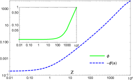
(a)  Specific case of $\omega_{b}=-1$ with $U(\phi)=\phi^{0.5}$

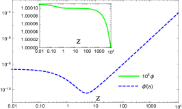
(b)  Specific case of $\omega_{b}=1/3$ with $U(\phi)=\phi^{2}$

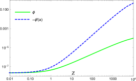
(c)  Specific case of $\omega_{b}=0$ with $U(\phi)=\phi^{2}$

Figure 1: The behaviors of $\phi$ and $\phi^{\prime}(a)$ vs $z$ for the specific case of $\omega_{b}=-1$, $\omega_{b}=1/3$, and $\omega_{b}=0$, respectively. Note that both horizontal and vertical axes are logarithmic.

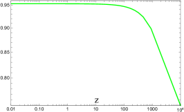
(a)  $\rho/3H_{0}^{2}$ vs $z$

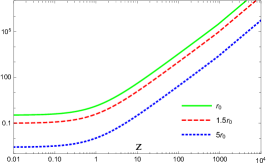
(b)  $\lvert\rho-\tau\rvert/3H_{0}^{2}$ vs $z$

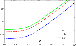
(c)  $(\rho+p)/3H_{0}^{2}$ vs $z$

Figure 2: The behaviors of $\rho$, $\rho-\tau$ (which is negative) and $\rho+p$, respectively, versus $z$ for different values of $r$ for $\omega_{b}=-1$ with $U(\phi)=\phi^{0.5}$. Note that both horizontal and vertical axes are logarithmic, except for the vertical axis of Fig. 2(a).

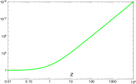
(a)  $\rho/3H_{0}^{2}$ vs $z$

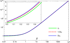
(b)  $(\rho-\tau)/3H_{0}^{2}$ vs $z$

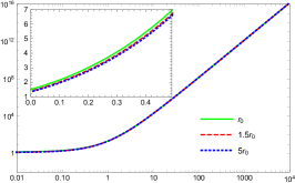
(c)  $(\rho+p)/3H_{0}^{2}$ vs $z$

Figure 3: The behaviors of $\rho$, $\rho-\tau$ and $\rho+p$, respectively, versus $z$ for different values of $r$ in the specific case of $\omega_{b}=1/3$ with $U(\phi)=\phi^{2}$. Note that both the horizontal and vertical axes are logarithmic.

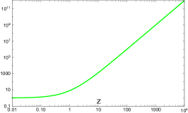
(a)  $\rho/3H_{0}^{2}$ vs $z$

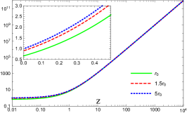
(b)  $(\rho-\tau)/3H_{0}^{2}$ vs $z$

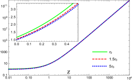
(c)  $(\rho+p)/3H_{0}^{2}$ vs $z$

Figure 4: The behaviors of $\rho$, $\rho-\tau$ and $\rho+p$, respectively, versus $z$ for different values of $r$ in the specific case of $\omega_{b}=0$ with $U(\phi)=\phi^{2}$. Both horizontal and vertical axes are logarithmic.

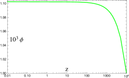
(a)  $\phi$ vs $z$

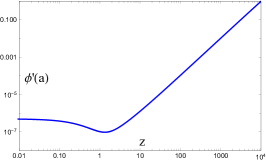
(b)  $\phi^{\prime}(a)$ vs $z$

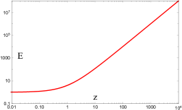
(c)  $E$ vs $z$

Figure 5: The behaviors of $\phi$, $\phi^{\prime}(a)$ and $E$ vs $z$ for the traceless EMT case with $U(\phi)=\phi^{2}$. Note that both horizontal and vertical axes are logarithmic, except for the vertical axis of Fig. 5(a). See the text for more details.

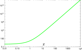
(a)  $\rho/3H_{0}^{2}$ vs $z$

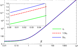
(b)  $(\rho-\tau)/3H_{0}^{2}$ vs $z$

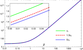
(c)  $(\rho+p)/3H_{0}^{2}$ vs $z$

Figure 6: The behaviors of $\rho$, $\rho-\tau$ and $\rho+p$, respectively, versus $z$ for different values of $r$ for a wormhole with traceless EMT with $U(\phi)=\phi^{2}$. Both horizontal and vertical axes are logarithmic.

In this section, we analyse evolving traversable wormhole geometries for the specific parameters $\omega_{b}=(-1,1/3,0)$ considered above, as well as evolving wormholes with a traceless EMT, and study the NEC and WEC for the solutions obtained.

Before going on further, we would like to comment on the potential for the scalar field $U(\phi)$ and its effects on the results. As Eqs. (29) and (30) (and (21)-(23)) show, the quantities $\rho-\tau$ and $\rho+p$ (and consequently the NEC) are independent of the scalar field potential. However, it affects the behavior of $\rho$. We will consider a power law potential for scalar field $U(\phi)=\phi^{\alpha}$. There are some reasonable choice for $\alpha$, such as $\alpha=2$ and $\alpha=4$, inspired by a mass term and the Higgs potential, respectively. In fact, we emphasize that all the results below hold qualitatively for potentials of the form $\phi^{2}$ and $\phi^{4}$. For the sake of economy, we will present the results for the quadratic case, $U(\phi)=\phi^{2}$. In addition to this, to verify that other choices for $\alpha$ could also present reliable results, we consider the specific choice $\alpha=0.5$ in one of the cases.

III.1 Specific case: $\omega_{b}=-1$

Here, we consider the specific case $\omega_{b}=-\tau_{b}/\rho_{b}=-1$ with $U\left(\phi\right)=V\left(\phi\right)/3H_{0}^{2}=\phi^{0.5}$. Figure 1(a) depicts the behaviors of $\phi$ and $\phi^{\prime}$ with respect to the redshift $z$ $(=1/a-1)$. In Fig. 2, the behaviors of $\rho$, $\rho-\tau$ and $\rho+p$ versus $z$ for different values of $r$ are shown. As one can see, $\rho-\tau$ is negative throughout the entire evolution. We emphasize that we have imposed different possible initial values and obtained the same result. Note that one may justify this outcome in the following manner. For this case with $\omega_{b}=-1$, Eq. (29) reduces to

$$\frac{\rho-\tau}{3H_{0}^{2}}=-\frac{\left(1+\phi(a)\right)r_{0}}{3a^{2}H_{0}^{2}r^{3}}+a^{2}\left(\frac{\phi^{\prime 2}(a)}{2\phi(a)}-\frac{\phi^{\prime\prime}(a)}{3}\right).$$ (31)

Since $a\leq 1$, the term with a coefficient $1/a^{2}$ is dominant. This term is therefore negative, rendering $\rho-\tau$ negative. Thus, for this specific case, both the NEC and the WEC are violated.

III.2 Specific case: $\omega_{b}=1/3$

Figure 1(b) illustrates the behavior of $\phi$ and $\phi^{\prime}$ versus $z$ for the specific case $\omega_{b}=1/3$. For this case, $E=a^{-2}$, $a(t)\propto t^{1/2}$ and we consider $U\left(\phi\right)=\phi^{2}$. The behaviors of $\rho$, $\rho-\tau$ and $\rho+p$ with respect to the redshift $z$ for different values of $r$ are displayed in Fig. 3, which shows explicitly that these quantities decrease as time evolves. However, they remain positive at all times and consequently the NEC and WEC are always satisfied. This occurs for the wormhole throat as well as for other wormhole radii. It is interesting to note that at a specified time/redshift, the quantity $\rho-\tau$ increases for increasing values of the radius, and the minimum value corresponds to the throat, as depicted by Fig. 3(b). On the other hand, $\rho+p$ decreases for increasing values of the radius, and has a maximum at the throat (Fig. 3(c)).

III.3 Specific case: $\omega_{b}=0$

Here we intend to study the energy conditions for the case $\omega_{b}=0$, for which $E=a^{-3/2}$ and $a(t)\propto t^{2/3}$. One can verify the behaviors of the scalar field $\phi$ and its derivative with respect to $a$ as functions of the redshift $z$ in Fig. 1(c), where we consider the power law potential corresponding to scalar field as $U\left(\phi\right)=\phi^{2}$. The energy conditions are depicted in Fig. 4, where one verifies that $\rho$, $\rho-\tau$ and $\rho+p$ are positive at all times and for different values of spatial coordinate $r$. These quantities are also decreasing (increasing) functions with respect to time (redshift). Thus, the NEC and WEC are always satisfied for all wormhole radii including the wormhole throat. The behaviors of $\rho-\tau$ and $\rho+p$ at a specified time/redshift are analogous to the previous case with $\omega_{b}=1/3$, namely, the quantity $\rho-\tau$ ($\rho+p$) increases (decreases) for increasing values of the radius (see Figs. 4(b) and 4(c)).

III.4 Wormholes with traceless EMT

In this subsection, we consider the traceless energy-momentum tensor, with $T=-\rho-\tau+2p=0$, which taking into account the dimensionless quantities defined above, provides the following differential equation

$$-3a^{2}E(a)^{2}\left[\phi^{\prime\prime}(a)-\frac{\phi^{\prime}(a)^{2}}{2\phi(a)}\right]-3aE(a)\big{[}aE^{\prime}(a)$$

$$+4E(a)\big{]}\phi^{\prime}(a)-6E(a)\left[aE^{\prime}(a)+2E(a)\right]$$

$$\times\left[1+\phi(a)\right]+6U(\phi)=0.$$ (32)

Here, we solve the system of coupled differential equations (26) and (III.4), for $\phi$ and $E$, numerically. The behaviors of $\phi$, $\phi^{\prime}$ and $E$ versus $z$, taking into account the choice $U\left(\phi\right)=\phi^{2}$, are shown in Fig. 5. Note that $E$ tends to unity at the present time ($z\rightarrow 0$), as expected (Fig. 5(c)). In Fig. 6, the behaviors of $\rho$, $\rho-\tau$ and $\rho+p$, with respect to $z$ for different values of $r$ are displayed. Note that $\rho$, $\rho-\tau$ and $\rho+p$ are decreasing (increasing) functions of time (redshift) and are positive for all radii, as time evolves. Thus, the NEC and WEC are satisfied at all times. Moreover, as shown in Figs. 6(b) and 6(c), the qualitative behaviors of $\rho-\tau$ and $\rho+p$ with respect to $r$ is analogous to the previous two cases, namely, $\omega_{b}=1/3$ and $\omega_{b}=0$, where the quantity $\rho-\tau$ ($\rho+p$) has a minimum (maximum) value at throat.

IV Discussion and Conclusion

In the present paper, we have studied the evolution of dynamic traversable wormhole geometries in a FLRW background in the context of hybrid metric-Palatini gravity. This theory, which recently attracted much attention, consists of a hybrid combination of metric and Palatini terms and is capable of avoiding several of the problematic issues associated to each of the metric or Palatini formalisms (for more details, we refer the reader to Refs. Capozziello:2015lza ; Harko:2018ayt ; Harko:2020ibn ). For the evolving wormholes, we presented the components of the energy-momentum tensor that supports these geometries in terms of the model’s functions, namely, the scalar field, the scale factor and the shape function (we considered a zero redshift function, for simplicity). Furthermore, we found specific wormhole solutions by considering a barotropic equation of state for the background matter, i.e., $\tau_{b}=-\omega_{b}\rho_{b}$, and considered particular equation of state parameters.

More specifically, we showed that for the specific cases of $\omega_{b}=1/3$ and $\omega_{b}=0$, the entire wormhole matter satisfies the NEC and WEC for all times. The latter cases are similar to the wormhole geometries analysed in the presence of pole dark energy KordZangeneh:2020jio , however, there the WEC is violated at late times, i.e., the energy density becomes negative. Thus, the present results outlined in this work strengthen the varying dark energy models and may suggest that hybrid metric-Palatini gravity is a rather more promising model to explore. In addition to the barotropic equation of state, we also studied evolving wormhole geometries supported by the matter with a traceless EMT. For this specific geometry, we discovered that both the NEC and the WEC are satisfied at all times as well. These results are extremely promising as they build on previous work that consider that the energy conditions may be satisfied in specific flashes of time Kar:1994tz ; Kar:1995ss .

An interesting astrophysical observational aspect on how to detect these wormholes would be to analyse the physical properties and characteristics of matter forming thin accretion disks around the wormhole geometries analysed in this work, much in the spirit of the analysis carried out in Refs. Harko:2008vy ; Harko:2009xf ; Harko:2009gc ; Harko:2017fra . In fact, specific signatures could appear in the electromagnetic spectrum, thus leading to the possibility of distinguishing these wormhole geometries by using astrophysical observations of the emission spectra from accretion disks. This would be an interesting avenue of research to explore.

- (1) S. Perlmutter et al. [Supernova Cosmology Project], “Measurements of and from 42 high redshift supernovae,” Astrophys. J. 517, 565-586 (1999) [arXiv:astro-ph/9812133 [astro-ph]].
- (2) A. G. Riess et al. [Supernova Search Team], “Observational evidence from supernovae for an accelerating universe and a cosmological constant,” Astron. J. 116, 1009-1038 (1998) [arXiv:astro-ph/9805201 [astro-ph]].
- (3) S. M. Carroll, “The Cosmological constant,” Living Rev. Rel. 4, 1 (2001) [arXiv:astro-ph/0004075 [astro-ph]].
- (4) S. Nojiri and S. D. Odintsov, “Unified cosmic history in modified gravity: from F(R) theory to Lorentz non-invariant models,” Phys. Rept. 505, 59-144 (2011) [arXiv:1011.0544 [gr-qc]].
- (5) T. P. Sotiriou and V. Faraoni, “f(R) Theories Of Gravity,” Rev. Mod. Phys. 82, 451-497 (2010) [arXiv:0805.1726 [gr-qc]].
- (6) S. Capozziello and M. De Laurentis, “Extended Theories of Gravity,” Phys. Rept. 509, 167-321 (2011) [arXiv:1108.6266 [gr-qc]].
- (7) P. Avelino, T. Barreiro, C. S. Carvalho, A. da Silva, F. S. N. Lobo, P. Martin-Moruno, J. P. Mimoso, N. J. Nunes, D. Rubiera-Garcia and D. Saez-Gomez, et al. “Unveiling the Dynamics of the Universe,” Symmetry 8, no.8, 70 (2016) [arXiv:1607.02979 [astro-ph.CO]].
- (8) F. S. N. Lobo, “The Dark side of gravity: Modified theories of gravity,” [arXiv:0807.1640 [gr-qc]].
- (9) K. Bamba and S. D. Odintsov, “Inflationary cosmology in modified gravity theories,” Symmetry 7 (2015) no.1, 220-240 [arXiv:1503.00442 [hep-th]].
- (10) S. Nojiri, S. D. Odintsov and V. K. Oikonomou, “Modified Gravity Theories on a Nutshell: Inflation, Bounce and Late-time Evolution,” Phys. Rept. 692 (2017), 1-104 [arXiv:1705.11098 [gr-qc]].
- (11) E. J. Copeland, M. Sami and S. Tsujikawa, “Dynamics of dark energy,” Int. J. Mod. Phys. D 15 (2006), 1753-1936 [arXiv:hep-th/0603057 [hep-th]].
- (12) G. W. Horndeski, “Second-order scalar-tensor field equations in a four-dimensional space,” Int. J. Theor. Phys. 10 (1974), 363-384
- (13) C. Deffayet, X. Gao, D. A. Steer and G. Zahariade, “From k-essence to generalised Galileons,” Phys. Rev. D 84 (2011), 064039 [arXiv:1103.3260 [hep-th]].
- (14) C. Wetterich, “Cosmology and the Fate of Dilatation Symmetry,” Nucl. Phys. B 302, 668-696 (1988) [arXiv:1711.03844 [hep-th]].
- (15) B. Ratra and P. J. E. Peebles, “Cosmological Consequences of a Rolling Homogeneous Scalar Field,” Phys. Rev. D 37, 3406 (1988).
- (16) R. R. Caldwell, R. Dave and P. J. Steinhardt, “Cosmological imprint of an energy component with general equation of state,” Phys. Rev. Lett. 80, 1582-1585 (1998) [arXiv:astro-ph/9708069 [astro-ph]].
- (17) I. Zlatev, L. M. Wang and P. J. Steinhardt, “Quintessence, cosmic coincidence, and the cosmological constant,” Phys. Rev. Lett. 82, 896-899 (1999) [arXiv:astro-ph/9807002 [astro-ph]].
- (18) C. Armendariz-Picon, T. Damour and V. F. Mukhanov, “k - inflation,” Phys. Lett. B 458, 209-218 (1999) [arXiv:hep-th/9904075 [hep-th]].
- (19) C. Armendariz-Picon, V. F. Mukhanov and P. J. Steinhardt, “A Dynamical solution to the problem of a small cosmological constant and late time cosmic acceleration,” Phys. Rev. Lett. 85, 4438-4441 (2000) [arXiv:astro-ph/0004134 [astro-ph]].
- (20) C. Armendariz-Picon, V. F. Mukhanov and P. J. Steinhardt, “Essentials of k essence,” Phys. Rev. D 63, 103510 (2001) [arXiv:astro-ph/0006373 [astro-ph]].
- (21) M. C. Bento, O. Bertolami and A. A. Sen, “Generalized Chaplygin gas, accelerated expansion and dark energy matter unification,” Phys. Rev. D 66, 043507 (2002) [arXiv:gr-qc/0202064 [gr-qc]].
- (22) K. Arun, S. B. Gudennavar and C. Sivaram, “Dark matter, dark energy, and alternate models: A review,” Adv. Space Res. 60, 166-186 (2017) [arXiv:1704.06155 [physics.gen-ph]].
- (23) A. G. Cohen, D. B. Kaplan and A. E. Nelson, “Effective field theory, black holes, and the cosmological constant,” Phys. Rev. Lett. 82, 4971-4974 (1999) [arXiv:hep-th/9803132 [hep-th]].
- (24) A. N. Tawfik and E. A. El Dahab, “Review on Dark Energy Models,” Grav. Cosmol. 25, no.2, 103-115 (2019).
- (25) G. J. Olmo, “Palatini Approach to Modified Gravity: f(R) Theories and Beyond,” Int. J. Mod. Phys. D 20, 413-462 (2011) [arXiv:1101.3864 [gr-qc]].
- (26) T. Harko, T. S. Koivisto, F. S. N. Lobo and G. J. Olmo, “Metric-Palatini gravity unifying local constraints and late-time cosmic acceleration,” Phys. Rev. D 85, 084016 (2012) [arXiv:1110.1049 [gr-qc]].
- (27) S. Capozziello and S. Tsujikawa, “Solar system and equivalence principle constraints on f(R) gravity by chameleon approach,” Phys. Rev. D 77 (2008), 107501 [arXiv:0712.2268 [gr-qc]].
- (28) J. Khoury and A. Weltman, “Chameleon cosmology,” Phys. Rev. D 69 (2004), 044026 [arXiv:astro-ph/0309411 [astro-ph]].
- (29) N. A. Lima, “Dynamics of Linear Perturbations in the hybrid metric-Palatini gravity,” Phys. Rev. D 89, no.8, 083527 (2014) [arXiv:1402.4458 [astro-ph.CO]].
- (30) N. A. Lima and V. S.-Barreto, “Constraints on Hybrid Metric-palatini Gravity from Background Evolution,” Astrophys. J. 818, no.2, 186 (2016) [arXiv:1501.05786 [astro-ph.CO]].
- (31) S. Capozziello, T. Harko, T. S. Koivisto, F. S. N. Lobo and G. J. Olmo, “Hybrid metric-Palatini gravity,” Universe 1, no.2, 199-238 (2015) [arXiv:1508.04641 [gr-qc]].
- (32) T. Harko and F. S. N. Lobo, Extensions of Gravity: Curvature-Matter Couplings and Hybrid Metric-Palatini Theory, Cambridge Monographs on Mathematical Physics, Cambridge, Cambridge University Press (2018).
- (33) T. Harko and F. S. N. Lobo, “Beyond Einstein’s General Relativity: Hybrid metric-Palatini gravity and curvature-matter couplings,” to appear in IJMPD [arXiv:2007.15345 [gr-qc]].
- (34) S. Capozziello, T. Harko, T. S. Koivisto, F. S. N. Lobo and G. J. Olmo, “The virial theorem and the dark matter problem in hybrid metric-Palatini gravity,” JCAP 07, 024 (2013) [arXiv:1212.5817 [physics.gen-ph]].
- (35) S. Capozziello, T. Harko, T. S. Koivisto, F. S. N. Lobo and G. J. Olmo, “Galactic rotation curves in hybrid metric-Palatini gravity,” Astropart. Phys. 50-52, 65-75 (2013) [arXiv:1307.0752 [gr-qc]].
- (36) S. Capozziello, T. Harko, F. S. N. Lobo and G. J. Olmo, “Hybrid modified gravity unifying local tests, galactic dynamics and late-time cosmic acceleration,” Int. J. Mod. Phys. D 22, 1342006 (2013) [arXiv:1305.3756 [gr-qc]].
- (37) S. Capozziello, T. Harko, T. S. Koivisto, F. S. N. Lobo and G. J. Olmo, “Cosmology of hybrid metric-Palatini f(X)-gravity,” JCAP 04, 011 (2013) [arXiv:1209.2895 [gr-qc]].
- (38) S. Carloni, T. Koivisto and F. S. N. Lobo, “Dynamical system analysis of hybrid metric-Palatini cosmologies,” Phys. Rev. D 92, no.6, 064035 (2015) [arXiv:1507.04306 [gr-qc]].
- (39) S. Capozziello, T. Harko, T. S. Koivisto, F. S. N. Lobo and G. J. Olmo, “Hybrid theories, local constraints, and cosmic speedup,” [arXiv:1301.2209 [gr-qc]].
- (40) C. G. Böhmer, F. S. N. Lobo and N. Tamanini, “Einstein static Universe in hybrid metric-Palatini gravity,” Phys. Rev. D 88, no.10, 104019 (2013) [arXiv:1305.0025 [gr-qc]].
- (41) Q. M. Fu, L. Zhao, B. M. Gu, K. Yang and Y. X. Liu, “Hybrid metric-Palatini brane system,” Phys. Rev. D 94, no.2, 024020 (2016) [arXiv:1601.06546 [gr-qc]].
- (42) J. L. Rosa, D. A. Ferreira, D. Bazeia and F. S. N. Lobo, “Thick brane structures in generalized hybrid metric-Palatini gravity,” [arXiv:2010.10074 [gr-qc]].
- (43) K. A. Bronnikov, “Spherically symmetric black holes and wormholes in hybrid metric-Palatini gravity,” Grav. Cosmol. 25, 331-341 (2019) [arXiv:1908.02012 [gr-qc]].
- (44) C. Y. Chen, Y. H. Kung and P. Chen, “Black Hole Perturbations and Quasinormal Modes in Hybrid Metric-Palatini Gravity,” [arXiv:2010.07202 [gr-qc]].
- (45) J. L. Rosa, J. P. S. Lemos and F. S. N. Lobo, “Stability of Kerr black holes in generalized hybrid metric-Palatini gravity,” Phys. Rev. D 101, 044055 (2020) [arXiv:2003.00090 [gr-qc]].
- (46) K. A. Bronnikov, S. V. Bolokhov and M. V. Skvortsova, “Hybrid metric-Palatini gravity: black holes, wormholes, singularities and instabilities,” Grav. Cosmol. 26, no.3, 212-227 (2020) [arXiv:2006.00559 [gr-qc]].
- (47) B. Danila, T. Harko, F. S. N. Lobo and M. K. Mak, “Hybrid metric-Palatini stars,” Phys. Rev. D 95, no.4, 044031 (2017) [arXiv:1608.02783 [gr-qc]].
- (48) K. A. Bronnikov, S. V. Bolokhov and M. V. Skvortsova, “Hybrid metric-Palatini gravity: Regular stringlike configurations,” Universe 6, 172 (2020) [arXiv:2009.03952 [gr-qc]].
- (49) T. Harko, F. S. N. Lobo and H. M. R. da Silva, “Cosmic stringlike objects in hybrid metric-Palatini gravity,” Phys. Rev. D 101, no.12, 124050 (2020) [arXiv:2003.09751 [gr-qc]].
- (50) N. Avdeev, P. Dyadina and S. Labazova, “Test of hybrid metric-Palatini -gravity in binary pulsars,” [arXiv:2009.11156 [gr-qc]].
- (51) J. L. Rosa, J. P. S. Lemos and F. S. N. Lobo, “Wormholes in generalized hybrid metric-Palatini gravity obeying the matter null energy condition everywhere,” Phys. Rev. D 98, no.6, 064054 (2018) [arXiv:1808.08975 [gr-qc]].
- (52) S. Capozziello, T. Harko, T. S. Koivisto, F. S. N. Lobo and G. J. Olmo, “Wormholes supported by hybrid metric-Palatini gravity,” Phys. Rev. D 86, 127504 (2012) [arXiv:1209.5862 [gr-qc]].
- (53) M. S. Morris and K. S. Thorne, “Wormholes in space-time and their use for interstellar travel: A tool for teaching general relativity,” Am. J. Phys. 56, 395-412 (1988).
- (54) M. S. Morris, K. S. Thorne and U. Yurtsever, “Wormholes, Time Machines, and the Weak Energy Condition,” Phys. Rev. Lett. 61, 1446-1449 (1988).
- (55) S. Kar, “Evolving wormholes and the weak energy condition,” Phys. Rev. D 49, 862-865 (1994).
- (56) S. Kar and D. Sahdev, “Evolving Lorentzian wormholes,” Phys. Rev. D 53, 722 (1996) [arXiv:gr-qc/9506094 [gr-qc]].
- (57) M. Visser, Lorentzian wormholes: From Einstein to Hawking, AIP press, New York (1995).
- (58) F. S. N. Lobo, Wormholes, Warp Drives and Energy Conditions, Fundam. Theor. Phys. 189, Springer, Switzerland (2017).
- (59) T. A. Roman, “Inflating Lorentzian wormholes,” Phys. Rev. D 47 (1993), 1370-1379 [arXiv:gr-qc/9211012 [gr-qc]].
- (60) L. A. Anchordoqui, D. F. Torres, M. L. Trobo and S. E. Perez Bergliaffa, “Evolving wormhole geometries,” Phys. Rev. D 57, 829-833 (1998) [arXiv:gr-qc/9710026 [gr-qc]].
- (61) A. V. B. Arellano and F. S. N. Lobo, “Evolving wormhole geometries within nonlinear electrodynamics,” Class. Quant. Grav. 23, 5811-5824 (2006) [arXiv:gr-qc/0608003 [gr-qc]].
- (62) E. Ebrahimi and N. Riazi, “(n+1)-Dimensional Lorentzian Wormholes in an Expanding Cosmological Background,” Astrophys. Space Sci. 321, 217-223 (2009) [arXiv:0905.3882 [hep-th]].
- (63) E. Ebrahimi and N. Riazi, “Expanding (n+1)-Dimensional Wormhole Solutions in Brans-Dicke Cosmology,” Phys. Rev. D 81, 024036 (2010) [arXiv:0905.4116 [hep-th]].
- (64) M. R. Bordbar and N. Riazi, “Time-dependent wormhole in an inhomogeneous spherically symmetric space time with a cosmological constant,” Astrophys. Space Sci. 331, 315-320 (2011).
- (65) S. N. Sajadi and N. Riazi, “Expanding lorentzian wormholes in gravity,” Prog. Theor. Phys. 126, 753-760 (2011).
- (66) M. Cataldo, F. Aróstica and S. Bahamonde, “(N+1)-dimensional Lorentzian evolving wormholes supported by polytropic matter,” Eur. Phys. J. C 73, no.8, 2517 (2013) [arXiv:1307.4122 [gr-qc]].
- (67) M. R. Setare and A. Sepehri, “Role of higher-dimensional evolving wormholes in the formation of a big rip singularity,” Phys. Rev. D 91, no.6, 063523 (2015) [arXiv:1612.05077 [gr-qc]].
- (68) S. Bhattacharya and S. Chakraborty, “ gravity solutions for evolving wormholes,” Eur. Phys. J. C 77, no.8, 558 (2017) [arXiv:1506.03968 [gr-qc]].
- (69) A. Ovgün, “Hawking’s universe as an evolving dark wormhole,” [arXiv:1803.04256 [physics.gen-ph]].
- (70) M. Cataldo, P. Labrana, S. del Campo, J. Crisostomo and P. Salgado, “Evolving Lorentzian wormholes supported by phantom matter with constant state parameters,” Phys. Rev. D 78, 104006 (2008) [arXiv:0810.2715 [gr-qc]].
- (71) M. Cataldo, S. del Campo, P. Minning and P. Salgado, “Evolving Lorentzian wormholes supported by phantom matter and cosmological constant,” Phys. Rev. D 79, 024005 (2009) [arXiv:0812.4436 [gr-qc]].
- (72) M. Cataldo and S. del Campo, “Two-fluid evolving Lorentzian wormholes,” Phys. Rev. D 85, 104010 (2012) [arXiv:1204.0753 [gr-qc]].
- (73) H. Maeda, T. Harada and B. J. Carr, “Cosmological wormholes,” Phys. Rev. D 79, 044034 (2009) [arXiv:0901.1153 [gr-qc]].
- (74) M. K. Zangeneh, F. S. N. Lobo and N. Riazi, “Higher-dimensional evolving wormholes satisfying the null energy condition,” Phys. Rev. D 90, no.2, 024072 (2014) [arXiv:1406.5703 [gr-qc]].
- (75) M. Kord Zangeneh, F. S. N. Lobo and H. Moradpour, “Evolving traversable wormholes satisfying the energy conditions in the presence of pole dark energy,” Phys. Dark Univ. 31 (2021), 100779 [arXiv:2008.04013 [gr-qc]].
- (76) M. R. Mehdizadeh, M. Kord Zangeneh and F. S. N. Lobo, “Einstein-Gauss-Bonnet traversable wormholes satisfying the weak energy condition,” Phys. Rev. D 91, no.8, 084004 (2015) [arXiv:1501.04773 [gr-qc]].
- (77) M. R. Mehdizadeh, M. Kord Zangeneh and F. S. N. Lobo, “Higher-dimensional thin-shell wormholes in third-order Lovelock gravity,” Phys. Rev. D 92, no.4, 044022 (2015) [arXiv:1506.03427 [gr-qc]].
- (78) M. Kord Zangeneh, F. S. N. Lobo and M. H. Dehghani, “Traversable wormholes satisfying the weak energy condition in third-order Lovelock gravity,” Phys. Rev. D 92, no.12, 124049 (2015) [arXiv:1510.07089 [gr-qc]].
- (79) F. Parsaei and S. Rastgoo, “Wormhole solutions with a polynomial equation-of-state and minimal violation of the null energy condition,” Eur. Phys. J. C 80, no.5, 366 (2020) [arXiv:1909.09899 [gr-qc]].
- (80) S. Capozziello, F. S. N. Lobo and J. P. Mimoso, “Energy conditions in modified gravity,” Phys. Lett. B 730, 280-283 (2014) [arXiv:1312.0784 [gr-qc]].
- (81) S. Capozziello, F. S. N. Lobo and J. P. Mimoso, “Generalized energy conditions in Extended Theories of Gravity,” Phys. Rev. D 91, no.12, 124019 (2015) [arXiv:1407.7293 [gr-qc]].
- (82) F. S. N. Lobo, “A General class of braneworld wormholes,” Phys. Rev. D 75, 064027 (2007) [arXiv:gr-qc/0701133 [gr-qc]].
- (83) F. S. N. Lobo and M. A. Oliveira, “Wormhole geometries in modified theories of gravity,” Phys. Rev. D 80, 104012 (2009) [arXiv:0909.5539 [gr-qc]].
- (84) N. M. Garcia and F. S. N. Lobo, “Wormhole geometries supported by a nonminimal curvature-matter coupling,” Phys. Rev. D 82, 104018 (2010) [arXiv:1007.3040 [gr-qc]].
- (85) N. Montelongo Garcia and F. S. N. Lobo, “Nonminimal curvature-matter coupled wormholes with matter satisfying the null energy condition,” Class. Quant. Grav. 28, 085018 (2011) [arXiv:1012.2443 [gr-qc]].
- (86) T. Harko, F. S. N. Lobo, M. K. Mak and S. V. Sushkov, “Modified-gravity wormholes without exotic matter,” Phys. Rev. D 87, no.6, 067504 (2013) [arXiv:1301.6878 [gr-qc]].
- (87) R. Korolev, F. S. N. Lobo and S. V. Sushkov, “General constraints on Horndeski wormhole throats,” Phys. Rev. D 101, no.12, 124057 (2020) [arXiv:2004.12382 [gr-qc]].
- (88) G. Antoniou, A. Bakopoulos, P. Kanti, B. Kleihaus and J. Kunz, “Novel Einstein-scalar-Gauss-Bonnet wormholes without exotic matter,” Phys. Rev. D 101, no.2, 024033 (2020) [arXiv:1904.13091 [hep-th]].
- (89) T. Tangphati, A. Chatrabhuti, D. Samart and P. Channuie, “Thin-shell wormholes in de Rham-Gabadadze-Tolley massive gravity,” Eur. Phys. J. C 80, no.8, 722 (2020) [arXiv:1912.12208 [gr-qc]].
- (90) E. Papantonopoulos and C. Vlachos, “Wormhole solutions in modified Brans-Dicke theory,” Phys. Rev. D 101, no.6, 064025 (2020) [arXiv:1912.04005 [gr-qc]].
- (91) A. Restuccia and F. Tello-Ortiz, “A new class of f(R)-gravity model with wormhole solutions and cosmological properties,” Eur. Phys. J. C 80, no.6, 580 (2020).
- (92) N. Godani and G. C. Samanta, “Traversable Wormholes in Gravity,” Eur. Phys. J. C 80, no.1, 30 (2020) [arXiv:2001.00010 [gr-qc]].
- (93) K. N. Singh, A. Banerjee, F. Rahaman and M. K. Jasim, “Conformally symmetric traversable wormholes in modified teleparallel gravity,” Phys. Rev. D 101, no.8, 084012 (2020) [arXiv:2001.00816 [gr-qc]].
- (94) A. Banerjee, M. K. Jasim and S. G. Ghosh, “Traversable wormholes in gravity satisfying the null energy condition with isotropic pressure,” [arXiv:2003.01545 [gr-qc]].
- (95) T. Tangphati, A. Chatrabhuti, D. Samart and P. Channuie, “Traversable wormholes in -massive gravity,” Phys. Rev. D 102, no.8, 084026 (2020) [arXiv:2003.01544 [gr-qc]].
- (96) I. Fayyaz and M. F. Shamir, “Wormhole Structures in Logarithmic-Corrected Gravity,” Eur. Phys. J. C 80, no.5, 430 (2020) [arXiv:2005.10023 [gr-qc]].
- (97) M. G. Richarte and C. Simeone, “Wormholes in Einstein-Born-Infeld theory,” Phys. Rev. D 80, 104033 (2009) [erratum: Phys. Rev. D 81, 109903 (2010)] [arXiv:2006.12272 [gr-qc]].
- (98) R. Ibadov, B. Kleihaus, J. Kunz and S. Murodov, “Wormholes in Einstein-scalar-Gauss-Bonnet theories with a scalar self-interaction potential,” Phys. Rev. D 102, no.6, 064010 (2020) [arXiv:2006.13008 [gr-qc]].
- (99) B. Lazov, P. Nedkova and S. Yazadjiev, “Uniqueness theorem for static phantom wormholes in Einstein-Maxwell-dilaton theory,” Phys. Lett. B 778, 408 (2018) [arXiv:1711.00290 [gr-qc]].
- (100) A. A. Kirillov and E. P. Savelova, “Wormhole as a possible accelerator of high-energy cosmic-ray particles,” Eur. Phys. J. C 80, 45 (2020) [arXiv:1902.05742 [gr-qc]].
- (101) D. Bak, C. Kim and S. H. Yi, “Experimental Probes of Traversable Wormholes,” JHEP 12, 005 (2019) [arXiv:1907.13465 [hep-th]].
- (102) Z. Xu, M. Tang, G. Cao and S. N. Zhang, “Possibility of traversable wormhole formation in the dark matter halo with istropic pressure,” Eur. Phys. J. C 80, 70 (2020).
- (103) K. Jusufi, P. Channuie and M. Jamil, “Traversable Wormholes Supported by GUP Corrected Casimir Energy,” Eur. Phys. J. C 80, 127 (2020) [arXiv:2002.01341 [gr-qc]].
- (104) F. S. N. Lobo, A. Simpson and M. Visser, “Dynamic thin-shell black-bounce traversable wormholes,” Phys. Rev. D 101, no.12, 124035 (2020) [arXiv:2003.09419 [gr-qc]].
- (105) F. Parsaei and N. Riazi, “Evolving wormhole in the braneworld scenario,” Phys. Rev. D 102, no.4, 044003 (2020) [arXiv:2004.01750 [gr-qc]].
- (106) V. De Falco, E. Battista, S. Capozziello and M. De Laurentis, “General relativistic Poynting-Robertson effect to diagnose wormholes existence: static and spherically symmetric case,” Phys. Rev. D 101, no.10, 104037 (2020) [arXiv:2004.14849 [gr-qc]].
- (107) R. Moti and A. Shojai, “Traversability of quantum improved wormhole solution,” Phys. Rev. D 101, no.12, 124042 (2020) [arXiv:2006.06190 [gr-qc]].
- (108) T. Berry, F. S. N. Lobo, A. Simpson and M. Visser, “Thin-shell traversable wormhole crafted from a regular black hole with asymptotically Minkowski core,” Phys. Rev. D 102, 064054 (2020) [arXiv:2008.07046 [gr-qc]].
- (109) M. Wielgus, J. Horak, F. Vincent and M. Abramowicz, “Reflection-asymmetric wormholes and their double shadows,” Phys. Rev. D 102, no.8, 084044 (2020) [arXiv:2008.10130 [gr-qc]].
- (110) S. Fallows and S. F. Ross, “Making near-extremal wormholes traversable,” [arXiv:2008.07946 [hep-th]].
- (111) J. Maldacena and A. Milekhin, “Humanly traversable wormholes,” [arXiv:2008.06618 [hep-th]].
- (112) F. S. N. Lobo and M. Visser, “Fundamental limitations on ‘warp drive’ spacetimes,” Class. Quant. Grav. 21, 5871-5892 (2004) [arXiv:gr-qc/0406083 [gr-qc]].
- (113) T. Harko, Z. Kovacs and F. S. N. Lobo, “Electromagnetic signatures of thin accretion disks in wormhole geometries,” Phys. Rev. D 78 (2008), 084005 [arXiv:0808.3306 [gr-qc]].
- (114) T. Harko, Z. Kovacs and F. S. N. Lobo, “Thin accretion disks in stationary axisymmetric wormhole spacetimes,” Phys. Rev. D 79 (2009), 064001 [arXiv:0901.3926 [gr-qc]].
- (115) T. Harko, Z. Kovacs and F. S. N. Lobo, “Can accretion disk properties distinguish gravastars from black holes?,” Class. Quant. Grav. 26 (2009), 215006 [arXiv:0905.1355 [gr-qc]].
- (116) T. Harko, Z. Kovács and F. S. N. Lobo, “Astrophysical Signatures of Thin Accretion Disks in Wormhole Spacetimes,” Fundam. Theor. Phys. 189 (2017), 63-88.