Spaces that can be ordered effectively: virtually free groups and hyperbolicity
Abstract.
We study asymptotic invariants of metric spaces, defined in terms of the travelling salesman problem, and our goal is to classify groups and spaces depending on how well they can be ordered in this context. We characterize virtually free groups as those admitting an order which has some efficiency on -point subsets. We show that all -hyperbolic spaces can be ordered extremely efficiently, for the question when the number of points of a subset tends to .
Key words and phrases:
hyperbolic space, hyperbolic groups, quasi-isometric invariants, uniform embeddings, space of ends, accessible groups2010 Mathematics Subject Classification:
20F65, 20F67,20F69, 20F181. Introduction
Given a metric space , we consider a finite subset of . We denote by the minimal length of a path which visits all points of . Now assume that is an order on (here and in the sequel we always assume that the orders are total orders). For a finite subset we consider the restriction of the order on , and enumerate the points of accordingly:
where . Here and in the sequel denotes the cardinality of the set . We denote by the length of the corresponding path
Definition 1.1.
Given an ordered metric space containing at least two points and , we define the order ratio function
If consists of a single point, then the supremum in the definition above is taken over an empty set. We use in this case the convention that for all .
Given an (unordered) metric space , we also define the order ratio function as
Given an algorithm to find an approximate solution of an optimization problem, the worst case of the ratio between the value provided by this algorithm and the optimal value is called the competitive ratio in computer science literature. We will recall below the setting of the universal travelling salesman problem. In this setting the function corresponds to the competitive ratio for -point subsets, in the situation when we do not require for a path to return to the starting point.
It can be shown that even in the case of a finite metric space, where the infimum in the definition above is clearly attained, the order that attains this minimum might depend on (see Remark 3.3).
We say that a metric space is uniformly discrete if there exists such that for all pairs of points the distance between and is at least . It is not difficult to see that the asymptotic class of the order ratio function behaves well with respect to quasi-isometries of uniformly discrete spaces, see Lemma 2.10.
This is no longer true without the assumption of uniform discreteness: and are in the same quasi-isometry class, but has a bounded order ratio function and the order ratio function of is unbounded; indeed, the latter space contains a square. It is shown in [HKL] that given any order on the square, there exist a finite subset of this lattice, such that the length of the path, associated to this order, is at least multiplied by the length of the optimal path. This implies an analogous bound in terms of the number of points of the subset rather than the size of the square: .
To avoid non-stability with respect to quasi-isometries, given a metric space , we can consider order ratio functions for -nets of (see Definition 2.5). It is not difficult to see (see Lemma 2.8) that the function is well-defined, up to a multiplicative constant, for being an -net of . This allows us to speak about the order ratio invariant of a metric space, see Definition 2.9 in Section 2.
In contrast with previous works on the competitive ratio of the universal travelling salesman problem ([bartholdiplatzman82, bertsimasgrigni, jiadoubling, HKL, Christodoulou, Schalekamp, bhalgatetal, gorodezkyetal, eades2]), we are interested not only in this asymptotic behaviour but also in particular values of . In the definition below we introduce the order breakpoint of an order :
Definition 1.2.
Let be a metric space, containing at least two points, and let be an order on . We say that the order breakpoint if is the smallest integer such that . If such does not exist, we say that . In particular, for a one-point space .
Given an (unordered) metric space , we define as the minimum over all orders on :
Given an order on , the order breakpoint describes the minimal value for which using this order as a universal order for the travelling salesman problem has some efficiency on -point subsets.
From the definition, it is clear that for any and it is easy to see that if is finite. In Section 3, Theorem 3.22 we evaluate the order breakpoint of finite graphs (containing edges): it is 2 for graphs homeomorphic to intervals, 3 for cactus graphs (see Definition 3.20) and 4 otherwise. In what concerns infinite graphs and metric spaces, it can be shown (see Lemma 4.1) that a metric space quasi-isometric to a geodesic one has unless it is bounded or quasi-isometric to a ray or to a line; metric on the vertex set of a graph has order breakpoint equal to 2 if and only if the graph is bounded, or quasi-isometric to a ray or line.
The order breakpoint is a quasi-isometric invariant for uniformly discrete metric spaces (see Lemma 2.13), hence it is well-defined for finitely generated groups. We characterize finitely generated groups with small () order breakpoint (in other words, groups that admit an order that has some efficiency on -point subsets):
Theorem A.
(= Thm 4.8) Let be a finitely generated group. Then is virtually free if and only if (in other words, if admits an order with ).
Using Stallings theorem and Dunwoody’s result about accessibility of finitely presented groups, we reduce the proof of Theorem A to Lemma 4.5, which provides a lower bound for for one-ended groups, and to Lemma 4.7 about mappings of trimino graphs to infinitely presented groups.
It seems interesting to better understand groups and spaces with given order breakpoint, in particular with . We mention that there are examples of metric spaces with arbitrarily large order breakpoint (see Remark 5.11).
Now we discuss the asymptotics of the order ratio function. The travelling salesman problem is a problem to find a cycle of minimal total length that visits each of given points. Bartholdi and Platzman introduced the idea to order all points of a metric space and then, given a -point subset, visit its points in the corresponding order [bartholdiplatzman82], [bartholdiplatzman89]. Such an approach is called the universal travelling salesman problem. (One of the motivations of Bartholdi and Platzman was that this approach works fast for subsets of a two-dimensional plane.) Their argument implies a logarithmic upper bound for the function .
For some metric spaces the function is even better. Namely, it is not difficult to show that , for all in the case of metric trees, see Thm 2 [Schalekamp] (an approriate order is shown on Figure 3.2, see also Corollary 3.5).
We prove that this best possible situation ( is bounded above by a constant) holds true for uniformly discrete hyperbolic spaces.
Theorem B.
(= Thm 5.10). Let be a -hyperbolic graph of bounded degree. Then there exists an order and a constant such that for all
It is essential that the constant depends on . In contrast with trees, this constant does not need to be bounded by and it can be arbitrarily large. In particular, for subsets of this constant depends on the dimension and the constants of uniform discreteness; if we fix and consider -nets, then this constant tends to infinity as the dimension of tends to infinity. In contrast with trees where the statement is true for any metric tree, it is essential in general to assume that the degree of the graph is bounded.
It is not difficult to see that some non-hyperbolic metric spaces also have bounded order ratio function; a particular family that arises from gluing together trees or hyperbolic spaces is studied in Subsection 5.3. So far we do not know whether a finitely generated non-hyperbolic group can have bounded ; for more related questions see the discussion at the end of Subsection 5.3.
We continue our study of the order ratio function and the order breakpoint in our subsequent paper [ErschlerMitrofanov2], where we show their relation with Assouad-Nagata dimension.
1.1. Plan of the paper
In Section we discuss basic properties of the order ratio function and the order breakpoint, their relation to quasi-isometries, uniform mappings and the notion of “snakes”.
In Section 3 we start with elementary examples of metric trees. We describe the asymptotics of the order ratio function for compositions of wedged sums of metric spaces. As a particular case we characterise the values of of finite graphs.
In Section 4 we study metric spaces and groups with small order breakpoint. The already mentioned Lemma 4.1 studies spaces with . Its proof – which uses a result of M. Kapovich about what are called -tripods – is given in Appendix . The main goal of the section is to prove Theorem 4.8 and thus characterise groups with .
The goal of Section 5 is the proof of Theorem B. Since by a theorem of Bonk and Schramm [bonkschramm] any -hyperbolic space of bounded geometry can be quasi-isometrically embedded into , taking in account Lemma 2.10 about quasi-isometric embeddings, the main goal in the proof of Theorem B is to prove it for an -net of . We do it by choosing an appropriate tiling of this space and considering a naturally associated tree; there is a family of hierarchical orders on this tree, and we choose any of these orders. While it is well-known that finite subsets of hyperbolic spaces can be well approximated by metric trees, we would like to stress that such an approximation does not provide a priori any upper bound for the order ratio function. We control the total length of piecewise-geodesic continuous paths associated to this order by bounding the number of tiles that are visited by such paths (here we use bounds on cones of a continuous path in a hyperbolic space, Lemma 5.7), and bounding the number of visits (see Lemma 5.6).
In subsection 5.3 we study (not necessarily hyperbolic) families of metric spaces with bounded .
Acknowledgements. We would like to thank Chien-Chung Huang and Kevin Schewior for references on the travelling salesman problem, and Nick Ramsey for conversations on first order logic. This project has received funding from the European Research Council (ERC) under the European Union’s Horizon 2020 research and innovation program (grant agreement No.725773).
Data availability. Data sharing not applicable to this article as no datasets were generated or analysed during the current study.
2. Preliminaries and basic properties
In this section we describe basic properties of the order ratio function and order breakpoint.
Lemma 2.1.
For any ordered metric space and any it holds that
Proof.
The first inequality is obvious. Let , and let be the diameter of . Then and . ∎
Definition 2.2.
Given metric spaces and , a map from to is a quasi-isometric embedding if there exist , such that for any it holds that
If is at bounded distance from , this map is called a quasi-isometry, and the spaces and are called quasi-isometric. If is bijective and , then the spaces are said to be bi-Lipschitz equivalent.
A significantly weaker condition is the following.
Definition 2.3.
Given metric spaces and , a map from to is an uniform embedding (also called coarse embedding) if there exist two non-decreasing functions , , with , such that
Definition 2.4.
We say that for a subset in a metric set is an -net if any point of is at distance at most from .
Definition 2.5.
We say that for a subset in a metric set is an -net if any point of is at distance at most from and the distance between any two distinct points of is at least .
It is clear that any -net of (in particular, any -net of ), endowed with the restriction of the metric of , is quasi-isometric to . Indeed, its embedding to satisfies the condition of Definition 2.2 with and . Observe also that is at distance of most from the image of this embedding. It is also clear from the definition that any -net is uniformly discrete. For convenience of the reader, we recall the following well-known observation.
Remark 2.6.
Let be a metric space. For any there exists an -net of .
Proof.
Consider a maximal, with respect to inclusion, subset of such that the distance between any two points is at least (in other words is a maximal with respect to inclusions -separated net of ). The maximality of this set guarantees that any point is at distance at most from . ∎
Definition 2.7.
Given (a not necessary injective) map and an order on let us say that an order on is a pullback of if the following holds: for any such that we have .
Note that a pullback of an order always exists: to construct a pullback it is (necessary and) sufficient to fix an order on each preimage for .
Lemma 2.8.
Let be a quasi-isometric embedding of a uniformly discrete space to a uniformly discrete space , then there is a constant such that if is an order on and is its pullback on , then for all
The constant can be chosen depending only on the quasi-isometry constants of and the uniform discreteness constants of and .
Proof.
There exists such that all distances between distinct points in and are greater than . Since is a quasi-isometry and since and are uniformly discrete, we know that there exists such that
if , and if .
Let , , , , . Let , . We know that , because the function is non-decreasing. If some path goes through all points of , the corresponding path in goes through all points of . Hence . The path that enumerates according to the order consists of preimages of edges of and edges with one point image. The first group of edges gives a contribution of towards , and the second group of edges gives . We also know that . Putting these inequalities together, we obtain
Therefore
and we can take . ∎
Lemma 2.8 above allows to speak about the order ratio invariant of a metric space.
In the definition below we say that two functions are equivalent up to a multiplicative constant if there exists such that and for all .
Definition 2.9.
For a metric space its order ratio invariant is defined to be the equivalence class, with respect to equivalence up to a multiplicative constant, of functions , where is some -net of .
In view of Lemma 2.8 we obtain the following.
Lemma 2.10.
For any metric space , is well-defined, and it is a quasi-isometric invariant of a metric space.
Proof.
If and are -nets of , they are quasi-isometric and from Lemma 2.8 it follows that and are equivalent up to a multiplicative constant. If two spaces are quasi-isometric then their -nets are also quasi-isometric.
∎
While specific values of the order ratio function can change under quasi-isometries, as can be easily seen already from finite space examples, the equality for given (the maximal possible value, see Lemma 2.1) is preserved under quasi-isometries, as we will see in Lemma 2.13.
Consider a sequence of points: .
Definition 2.11.
We call such sequence to be a snake on points, of diameter and of width , if the diameter of this set is and the maximal distance where and are of the same parity, is . For a snake on at least two points, we say that the ratio is the elongation of the snake. If , then the width of the snake is , and we say in this case that the elongation is infinite.
Lemma 2.12.
Let be a metric space, containing at least two points, and let be an order on and consider . The following conditions are equivalent:
-
(1)
-
(2)
There exist snakes on points in of arbitrarily large elongation.
Proof.
. Let be a snake of diameter and width . From the triangle inequality it follows that the distance between any consecutive points is greater than or equal to . This shows that . Observe also that , because we can pass first through all points with odd indexes and then all points with even indexes. Hence
that tends to as tends to . The other inequality comes from Lemma 2.1.
. We can assume that . Let , and .
Since and , we conclude that
-
•
and
-
•
.
The first inequality implies that for all , is close to the diameter of : .
The second inequality implies that for any triple of points of , the minimal sum of two pairwise distances is at most . If , then .
Applying these inequalities for the triple , we observe that . Observe that the shortest path joining , , can not be the path visiting them in this order , , . Indeed, the sum can not be the minimal sum of two pairwise distances from the triple, because .
This implies that the width of the snake is at most , and its elongation is greater than of equal than . ∎
Since a snake on points contains snakes on fewer points, it is clear that implies for all integers .
Lemma 2.13.
[Snakes, Order Breakpoint and quasi-isometries]
-
(1)
Let an integer be , let be a uniformly discrete space with and let be a quasi-isometric embedding of to a metric space . Then .
-
(2)
In particular, if and are quasi-isometric uniformly discrete metric spaces, then .
Proof.
(1) Observe that if , then by definition of order ratio function we have for any order on . If , then there exist an order such that . Let be a pullback of . Since , we know that admits a sequence of snakes on points with elongations that tend to infinity.
A snake on points in with large enough elongation maps to a snake on points in , and in particular these points are distinct. The argument is the same as in the beginning of the proof of Lemma 2.15 mutatis mutandis.
Since is a quasi-isometry, the length of is bounded from below by some affine function of the length of , and the width of is bounded from above by some affine function of the width of .
Because of the uniform discreteness, the widths of these snakes in are uniformly separated from zero, so their diameters tend to infinity. The diameter of is bounded below by some affine function of the diameter of , and the width of is bounded above by some affine function of the width of . As is uniformly discrete, and by restricting to snakes of large diameter, we can choose these affine functions to have ho additive constants. Since the elongations of the snakes tend to infinity, it follows that the elongations of the snakes tend to infinity, and this is in contradiction with the fact that .
(2) Follows from (1), because is the smallest integer such that . ∎
Now we introduce a strengthening of the condition . In contrast with the property of admitting snakes of large elongation, this property will be inherited by the images of uniform embeddings.
Definition 2.14.
We say that an ordered metric space admits an -sequence of snakes on points if it admits a sequence of snakes on points, in which the diameters of snakes tend to and the widths of all snakes are . If a sequence of snakes on points is an -sequence for some , we say that this sequence of snakes is an -sequence.
This notion allows us to obtain estimates for in the case when one metric space is uniformly embedded in another one.
Lemma 2.15.
Let and be metric spaces. Let be a uniform embedding of to , be an order on , and be its pullback on . Then if for some the ordered space admits an -sequence of snakes on points, then also admits such sequence of snakes and .
Proof.
Let be such that any two points at distance in map to a pair of distinct points in . Let be a snake in of diameter and width and let . Note that for any and of different parity. This means that
hence is a snake on points in .
Consider an -sequence of snakes in . Observe that its image under a uniform embedding is a sequence of -snakes in . We can conclude therefore that admits snakes on points of arbitrarily large elongation, and hence by Lemma 2.12 we know that . ∎
The following lemma implies that the order ratio function of a metric space is defined by the order ratio functions of all its finite subsets.
Lemma 2.16.
Let be a metric space. Consider a function and assume that for any finite subset there exists an order satisfying for all . Then there exists an order on satisfying for all .
Proof.
Indeed, we can take one constant symbol for each point of . Observe that for a binary predicate “”, the fact that it defines an order can be described by first order sentences. Also for any finite subset we forbid all its orders for which for some , this can also be described by a set of first order formulas. Then the statement of this lemma follows from the Compactness theorem. ∎
Note that for any finite metric space its is equal to . This means that the inequality does not follow from inequalities for finite subsets of . To prove that you also have to provide for all finite some uniform bound for elongations of snakes on points.
Now we give one more definition that will be used in later sections.
Definition 2.17.
Let be a set, be an order on and be a subset. We say that is convex with respect to if for all such that it can not be that and .
We give a lemma that provides a sufficient condition for the existence of an order where the sets of some given family are “convex”.
Lemma 2.18.
Let be a family of subsets of such that for any two sets either their intersection is empty, or one of the sets is contained in another one. Then there exists an order on such that all sets in are convex with respect to .
Proof.
For finite the claim can be proved by induction on the cardinality of . If (and hence ) then the statement is obvious. Inductive step: if there are no sets besides and in , then any order satisfies the desired conditions. Otherwise, let a set be maximal by inclusion in (we use the same letter for the space and here for the set containing all points of ) and let . Our assumption on and the maximality of implies that any , , is either a subset of or a subset of . Since , the induction hypothesis implies the existence of orders on and on such that for all sets of that are subsets of are convex with respect to . The required order can be constructed as follows: all elements of are than all elements of , and on for or .
Now consider the case when is not necessarily finite. We use again the Compactness theorem (similarly to the proof of Lemma 2.16) to make a reduction to the finite case. Consider constant symbols corresponding to points of and to the binary relation . Observe that the axioms of a relation to be an order and the condition in the definition of convex sets can be described by sentences of first order. Any finite collection of these sentences has a model by applying the lemma to finite subsets of , hence the whole collection of sentences has a model. ∎
Now we mention some examples of families of convex sets for metric spaces which we describe in the following sections.
-
(1)
For rooted trees we can choose an order such that all branches of the tree are convex with respect to the order (see Lemma 3.4.)
-
(2)
For the graph associated to a tiling of a hyperbolic space and the order, constructed in Section 5, the sets that correspond to branches of the corresponding tree are convex.
-
(3)
In Definition 3.16 we define Star orders for graphs endowed with edges. Star figures (union of a vertex and all the outgoing half-edges) are convex with respect to these orders.
In these examples we could find the orders by showing that the above mentioned sets satisfy the assumption of Lemma 2.18 and apply this lemma. We do not explain the details, since, as we have mentioned, we will describe these orders more explicitly in Sections 3, 5.
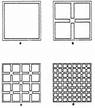
We already mentioned an order on a square, constructed by Bartholdi and Platzman. Now we describe explicitly another hierarchical order on the unit square.
This order also uses self-similarity in its construction, and we chose this particular order to guarantee that the squares (discussed below) are convex.
Example 2.19.
Let . For each point we consider the binary representations and of and correspondingly. Given , we define to be the number with binary representation . We define the order by setting . Then all parts that are obtained by splitting into equal squares are convex with respect to .
The figure below illustrates the order on these smaller squares.
3. Metric trees, acyclic gluings, finite graphs
In this section we describe first examples of evaluation of the order breakpoint and of asymptotic behaviour of the order ratio function. Some of these examples will be used in the following sections.
Lemma 3.1.
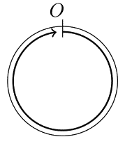
Let be a circle (with its inner metric). Then for all . More precisely, for any order of and any there exists a snake on points such that its points are located in -neighborhoods of two antipodal points of .
Proof.
Denote by the length of the circle. Let be a natural order on this circle (see Figure 3.1). Suppose that and . This means that the set lies on an arc of length . If this arc does not contain the point , then . If this arc contains , then . Hence for all .
Since the function is non-decreasing in , it is enough to prove that . We will show that for any order on and any there exist points , , such that and , i.e. is a snake of large elongation.
Take , . Consider points with , numbered with respect to the order . Consider a map from to the two point set which takes value at a point if the antipodal point to is -smaller than and otherwise. Clearly, the preimages of and are non-empty. Therefore, there exists an index (considered modulo ) such that , .
This means that and . If , then the snake has large elongation. Otherwise we take the snake . ∎
This lemma has a generalisation to spheres of dimension . For statements and applications we refer to Section in [ErschlerMitrofanov2].
A tripod is a metric space that consists of three segments meeting at one vertex.
Corollary 3.2.
Let be a tripod. Then . If is the minimal length of the three segments of , then for all and for any order of there exists a snake on three points, of diameter at least and of width at most .
Proof.
We can assume that all segments of the tripod have length . Consider to be a circle of length . There is a -Lipschitz map (see the figure below) such that any two antipodal points map to a pair of points at distance .
Let be an arbitrary order on and let be some pullback of to . From Lemma 3.1 we know that for any there are two antipodal points and points such that , . Here denotes an open ball of radius centered at .
We know that . Then and , and . Since is a pullback of we can conclude that . This implies the second claim of the Corollary, and in particular that . ∎
The following example shows that for some metric spaces the choice of an order that optimizes depends on .
Example 3.3 (Dependence of an optimal order on the number of points).
Let be a six point metric space, with the distance function described by the matrix
Observe that the pairwise distances take values between and , and hence satisfy the triangular inequality.
It can be checked that the only orders that minimize are and , but these two orders are not optimal for . It can be shown that the order satisfies .
3.1. Orders on trees. Hierarchical orders
Consider a finite directed rooted tree . The root of the tree is denoted by . Any vertex can be joined with the root by a unique directed path, and in particular each vertex has at most one parent. We assume that the direction on each edge is from the parent to its child.
We also assign to each edge some positive length, and this provides a structure of a metric space on the vertices of . We say that is an ascendant of if there exists a sequence of vertices , such that for each the vertex is a parent of .
Let be an order on the vertices of the rooted tree , defined as follows. First for any vertex we fix an arbitrary order on the children of this vertex. Now if a vertex is an ascendant of then . Otherwise consider paths of minimal length from to and : and . Observe that if neither is an ascendant of nor is an ascendant of , then there exists such that . Take minimal with this property and put if (in our fixed order on the children of ).
Any order obtained in this manner we call a rooted order. Let us say that a subset of a rooted tree is a branch if it consists of some vertex and all vertices such that is an ascendant of . We denote this subset .
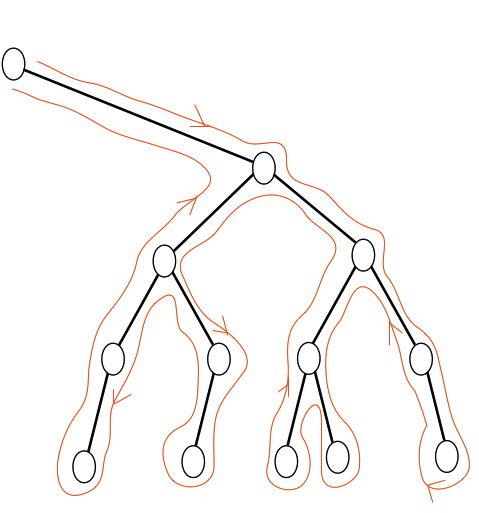
Let us say that an order on vertices of a rooted tree is hierarchical if the following holds. Suppose that and and belong to some branch. Then also belongs to this branch.
The existence of hierarchical orders can be deduced from Lemma 2.18. Without referring to this Lemma, it is also not difficult to see it more directly, in Lemma 3.4. Claim (1) of this Lemma is proven in Thm 2, [Schalekamp]. For the convenience of the reader we provide the proof.
Lemma 3.4.
Let be a rooted tree as above, then
-
(1)
For any and any rooted order it holds that
where is the set of vertices of .
-
(2)
Any rooted order is hierarchical.
Proof.
Let be a subset of vertices of , . Observe that any (possibly self-intersecting) continuous path passing through passes through all the vertices of the spanning tree of . Observe also that is at least the sum of the lengths of all edges in . It is clear that the restriction of to is a rooted order on .
Now consider a path through vertices of with respect to our order . Let us show that this path passes at most twice through each edge of the spanning tree, this would show that the length of this path is at most twice the length of the optimal tour. Without loss of generality we can assume that . We prove the claim by induction on the number of vertices of the tree . For each child of , consider the corresponding branch. The tour with respect to first visits , then one of its children and all points of its branch, then another child and all points of its branch. Observe that the edge from to any of its children is visited at most twice: once passing from to its child, and, possibly second time, after visiting all points of the branch of this child, before passing to another child of . Now observe that all edges not adjacent to are visited at most twice by induction hypothesis, applied to the branches of . So we have proved the first claim of the lemma.
Now let be a vertex of and be a branch. From the argument above it follows that the tour with respect to after visiting visits all points of , before visiting any other points (not in ). This implies the second claim of the lemma that the order is hierarchical. ∎
Recall that a metric space is a metric tree if it is a geodesic metric space which is -hyperbolic.
Corollary 3.5.
Let be a metric tree. Then there is some order such that for all .
Proof.
By Lemma 2.16 we know that if the statement that is true for any finite tree, then it is true for any metric tree. ∎
We say that an order on a metric tree is hierarchical if for any finite subset there is a choice of root (which includes a rooted tree structure on ) such that the restriction of to is hierarchical. Hierarchical orders always exist. To show this we can choose a point as the root and obtain an order by applying Lemma 2.18 to the collection that consists of all subsets such that is a component of for some and . Given a finite subset , we can choose the root of to be any closest point to . It is then not hard to show that the restriction of to is hierarchical. It can be shown that any hierarchical order satisfies the conclusion of Corollary 3.5, the proof is essentially the same as the proof of the first statement of Lemma 3.4.
Remark 3.6.
Let be a free group with a free generating set , . If we consider as a metric space with the word metric with respect to , then embeds isometrically into its Cayley graph, which is a metric tree. Corollary 3.5 implies that for all . Now we describe a more explicit order. Recall that each element of corresponds to a unique irreducible word in the alphabet . Choose an order on the set , then the lexicographic order on words on this alphabet provides an example of a hierarchical order on with for all .
3.2. Acyclic gluing of spaces
Let us say that a metric space is an acyclic gluing of metric spaces if it is obtained as follows. Consider a graph which is a tree (finite or infinite), vertices of which have labellings of two types: each vertex is either labelled by , for some or it is labelled by a one-point space . Each edge joins some and , and is labelled by a point .
Our space is obtained from a disjoint union of and points by gluing all to the points in corresponding .
A graph which is an acyclic gluing of circles and intervals is also called a cactus graph. An example of a space homeomorphic to a cactus graph, with only circles glued together, is shown on Figure 3.3. Observe, that a finite acyclic gluing can be obtained by a finite number of operations which take a wedge sum of two metric spaces.
We will describe a natural way to order points of if orders on are given.
For acyclic gluings it will be more natural to consider cyclic order ratio functions.
Definition 3.7.
Let be a metric space with an order . If is a finite subset of we denote by the minimal length of a closed path visiting all points of . We denote by the length of the closed path corresponding to the order : if the distance between the first and the last vertices of is equal to , then .
We define the cyclic order ratio function as
Lemma 3.8.
For any ordered metric space and any it holds that
Moreover if is odd, then the following conditions are equivalent:
-
(1)
-
(2)
There exist snakes on points in of arbitrarily large elongation
Proof.
The inequality is obvious. Let , , and let be the diameter of . Then and . This implies the inequality .
Let be odd and let be a snake of diameter and width . By the triangle inequality, for any we have and hence . It also holds that . If the snake has large elongation then is close to .
Now assume that a subset has diameter and is close to . Suppose that . The following argument is analogous to that in the proof of Lemma 2.12. It is easy to see that for any the distances and are close to , and is close to 0 (we assume here that ). We can deduce that the width of the snake is also close to 0, and has large elongation. ∎
The equivalence of and in the lemma above means that for odd , if and only if .
Definition 3.9.
Let be a metric space (or more generally a set) and be an order on . Suppose that is a disjoint union and that for any two points , we have . We define a new order on as follows: if or we put if . For any two points and we put . We say that is a cyclic shift of the order .
It is clear that for a given metric space the relation to be a cyclic shift is an equivalence relation on orders. For example, all clockwise orders of a circle with different starting points are cyclic shifts of each other. For a given metric space , an order and a point , there exists a unique cyclic shift such that is the minimal point for this order.
In the following two remarks we state straightforward properties of cyclic shifts and cyclic order ratio functions.
Remark 3.10.
If is a metric space endowed with an order , then for any finite subset of it holds that
It follows that for any
For any , if and only if .
Remark 3.11.
If is a cyclic shift of , then for any we have
In particular, taking in account the last claim of the previous remark if and only if .
Now given a family and a family of orders on these spaces , we consider a metric space which is an acyclic gluing of ordered spaces , . We define a family of clockwise orders on as follows. We assume below that the tree in the definition of acyclic gluing is finite (this is assumption is not essential). One way is to define such orders recursively: having already defined orders and on two metric spaces and , we will define an order on the wedge sum of and over a point . We choose any of the two ways to enumerate and , for example and . We use the notation that denotes by both a point in and one in .
Recall that for any point in any space, there is a cyclic shift that makes this point minimal. Let and be cyclic shifts of and respectively such that is the minimal point in and . Consider the order on a wedge sum of and , such that is a minimal point, then come all points of ordered as in and then all points of ordered as in . In such a way we construct recursively an order on an acyclic gluing. We say that such orders and any cyclic shift of these orders are clockwise orders on . Finally, if the tree in the definition of an acyclic gluing is infinite, we can say that an order on this space is a clockwise order if the restriction of this order to any finite (connected) acyclic gluing is a clockwise order.
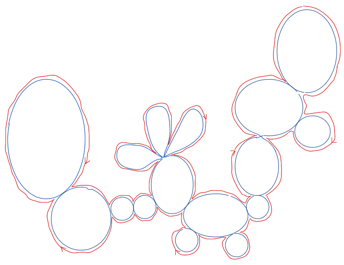
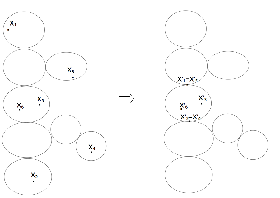
There is another way to formulate this definition and to visualize clockwise orders. Given an acyclic gluing of , , we consider circles , and choose a direction (clockwise order) on each . For all joint points on we consider points on enumerated in the same order, up to a cyclic shift, and we consider the corresponding acyclic gluing of . The clockwise order on an acyclic gluing of can be obtained in the following way. We construct a continuous embedding of in the plane in such a way that the image of is equal to its outer boundary, and the clockwise orientation of the boundary of the image of (in the plane) coincides with clockwise orientations of .
We choose a joint point (among joint points joining our circles) as a base point and consider an order corresponding to the first visit of a clockwise path in the plane, see Figure 3.3. For each point of we can associate an arc in . If is a joint point in , then it corresponds to a joint point in . We will use a convention that the initial point of an arc (with respect to the first visit of the clockwise path starting from ) is included in the arc and the last point of the arc is not included.
A clockwise order on can be described as follows. Take . First suppose that there exists such that . Observe that our choice of fixes a choice of a cyclic shift on the acyclic gluing of our circles (and in particular on ). This induces a choice of an acyclic shift also on . In case when there exists such that we compare with respect to the above mentioned cyclic shift of (on ). Finally, if there is no such that belong to the same , we consider corresponding arcs , , choose any point , and compare and in . If with respect the order in , then we say that
Now observe that a metric tree is an acyclic gluing of intervals, and recall that for all in this case. Here we prove a statement about general acyclic gluings.
Lemma 3.12.
Let be an acyclic gluing of ordered spaces , . Let be a clockwise order on . For all we have
If we allow metric spaces with infinite distances between some points, there is a way to define also in this more general setting (considering subsets with finite pairwise distances) and in this setting the lemma can be reformulated to claim that order ratio function of an acyclic gluing is the same as for the disjoint union of .
Proof.
It is obvious that the left hand side in the equation in the lemma is at least as large as the right hand side, so it is enough to prove that
To prove this inequality, we first observe that it is enough to prove this claim for finite acyclic gluings. We consider a finite set consisting of points . Consider a minimal (with respect to inclusion) acyclic gluing of , , containing . If are path-connected metric spaces, then observe that any continuous path passing through visits each , for . Even though are not assumed to be path-connected in general, for any two points we can consider a finite sequence of points , …, where depends on and , such that for any the points and belong to the same component , and the distance between and is
It is clear that such exist and we can choose the such that for these points are joint points in the acyclic gluing.
Now we choose a component , and consider the retract mapping that maps every point of to the nearest point of . It is clear that if then is a joint point. Observe, that the retract sends the clockwise order on to some (cyclic shift) of . More precisely, if we choose an arbitrary point that is not a joint point and consider the cyclic shift of , then for any two points we have .
Observe also that any closed path passing through () passes through all their images (). To be more precise, if are not necessarily geodesic, we use the same convention as before: by a path in we mean a sequence of points such that any two consecutive points are in the same component. We call such pairs of consecutive points jumps.
For the shortest closed path visiting all points of we consider all its jumps inside . These jumps form a cyclic tour visiting all the points of , and their total length is at least . Now we consider a tour of with respect to a clockwise order , and take all its “jumps” inside . They form a tour of with respect to and , and its length can be bounded from above as follows
Summing these inequalities over all and using the obvious inequality
we prove the claim of the lemma. ∎
In Remark 3.10 we mention that and are the same up to the multiplicative constant . So we get the following
Corollary 3.13.
Let be an acyclic gluing of ordered spaces , . Let be a clockwise order on . Then for any
As another corollary we obtain
Corollary 3.14.
Let be an acyclic gluing of ordered spaces , , and let be a clockwise order on . For a finite acyclic gluing if and only if for some it holds that . More generally, for a not necessarily finite acyclic gluing we have if and only if there is no uniform upper bound for all on elongations of snakes on points in .
Proof.
The “if” directions obviously follow from Lemma 2.12. Now suppose that for each the elongations of snakes on points in all are uniformly bounded from above. Using the upper bound for in terms of the elongations of snakes (see the proof of Lemma 3.8), we observe that there exists such that for any . Lemma 3.12 shows that , and the result follows from Lemmas 3.8 and 2.12. ∎
The following corollary is about for free product of groups. In the particular case of virtually free groups we will show later that they can be characterized as groups with small . In this corollary the metric associated to the groups is the word metric on the elements of these groups (we consider only vertices of Cayley graphs, not edges).
Corollary 3.15.
Let be a free product of groups and . If the maximum of , is odd, then is equal to this maximum. If the maximum is even, then is either equal to this maximum or the maximum plus one.
Proof.
Observe that the metric space associated to (that is, the word metric on this free product) is an acyclic gluing of metric spaces where each is isometric to or to . It is clear that . Let be an integer such that , then and . From Corollary 3.14 it follows that and . ∎
If we do not assume that the maximum is odd, the “plus one” in the formulation is essential. For example, and (see Lemma 4.1).
3.3. Order breakpoint of finite graphs.
In this subsection we consider both finite and infinite graphs, but the main goal is to classify finite graphs depending on their order breakpoints. Let be a graph, finite or infinite, with edges of length . We consider as a geodesic metric space with edges included. Given an order on the set of vertices of , we define an order on all points of as follows.
Definition 3.16.
Given an order on the set of vertices of , we define the order on . We subdivide each edge into two halves of length , and we assume that the middle point belongs to the half of if . We call a union of a vertex and all the outgoing half-edges a star figure. For each point in we have defined therefore the vertex (to the half-interval of which it belongs). If we put . On points with the same we consider a hierarchical order on the corresponding star figure, assuming that the vertex is smaller than the other points. So we have an order on the set of half-edges, and each half-edge is ordered by identifying it with the interval or , where 0 corresponds to the vertex.
A comment on the definition above: the choice to which half edge the middle point belongs, and the order we have chosen for half edges with a common vertex (the corresponding star figure) is not important. We have made this choice to fix an order on star figures which we will study in the sequel.
Lemma 3.17 below shows that for the asymptotic behaviour of the order ratio function it does not matter whether we consider the graph together with the edges or only the metric on the vertices. In a more general setting, the asymptotic behavior of the order ratio function depends on both the local and global geometry of the metric space.
Lemma 3.17.
For any graph and all it holds that
This lemma is proven by associating to a path in a path that passes through the centers of corresponding star figures. For details of the proof see Appendix A. We do not use this lemma in the sequel, but we will use some other properties of the orders.
It is clear that order breakpoint can change by applying operation: for example, of the tripod is while of the set of its four vertices is . However, this operation provides a bound on of the graph.
Lemma 3.18.
If is any (finite or infinite) graph, then is at most . In particular, if is a finite graph, then .
Proof.
Let be a constant such that any star figure does not admit snakes on points of elongation greater than with respect to the order (from the proof of Lemma 2.12 it follows that for any hierarchical order on a metric tree, the elongation of snakes on points is bounded by ). Let be such that does not admit snakes of arbitrarily large elongation on points. Let us show that does not admit snakes of arbitrarily large elongation on points. Suppose that this is not the case and admits such snakes. For each point of the snake , , consider the vertex such that belongs to the star figure of . If the elongation of the snake is , then it is clear that among the vertices there are at least two distinct points.
Let and be the diameter and the width of the snake , . First suppose that all , are distinct. Observe that . Indeed, , , belong to three distinct star figures, so not all the pairwise distances between these points can be less than . We can assume that the elongation of the snake is , hence . Observe that in this case the corresponding vertices of , , form a snake of diameter satisfying and of width . We see that under our assumption the elongation of the snake is at least of the elongation of .
Now observe that if there exist at least two points of the snake belonging to the same star figure , then (since the star figure is convex with respect to the order on ) there exist two points of indices of different parity belonging to . We see that . Assume that the elongation . We have , and . We conclude that all points of our snake are in the “extended” star figure with edges of length . We know that not all belong to , and that this star figure is convex with respect to the Star order. Thus, reversing if necessary our order we can assume that does not belong to this star figure. We know that the distance between and and between and is at most . This implies in particular that these points belong to the same edge of as .
If belongs to the same half-edge as , then, taking in account convexity of this half-edge, we conclude that also belong to the same half-edge. In this case the elongation of the -point snake is . Its diameter is and its width is , where and are the parameters of the initial snake. Hence , and the elongation of the initial snake is at most .
Finally, if does not belong to the same (external) half-edge as , then can not belong to the same interval as because the half edge is convex with respect to the order. Then and belong to the same half-edge. In this case we obtain a snake on points with elongation and again get a contradiction.
We have proved the first claim of the lemma. The second claim follows from the fist one, since it is clear that finite sets do not admit snakes on three points of large elongation.
∎
For the rest of this section, we assume that our graph is finite. As before, we consider a metric space of a finite graph , with edges (not only vertices) included.
Now we compute the order breakpoint for such graphs. It is clear that is equal to if is homeomorphic to an interval. We have seen already that is equal to for a circle or a tripod. We start with an example with . The domino graph is the graph with 6 vertices and 7 edges, shown at Figure 3.5.
Lemma 3.19.
[Order breakpoint of a domino graph] Let be a graph homeomorphic to the domino graph. Then for any order on , this graph admits snakes on points of large elongation. More precisely, for any there exists a snake on 4 points of diameter and of width at most .
Proof.
Consider two tripods and , with segments of length , with their joint vertices at and (see Figure 3.5). By Corollary 3.2 we know that in there exists a snake on three points of diameter at least and of width at most . Denote its points , , , here . Without loss of generality, the distance between and is . Observe that there is a continuous path from to any point of which stays at distance at least from . If equipped with our order does not admit snakes on points of width at most and diameter at least , we would see that any point on this continuous path stays (with respect to the order ) between and . This would show that all points of are between some two points of the first tripod . The same argument shows that all points of the first tripod are between some two points of the second one, and this contradiction implies the claim of the lemma. ∎
An argument similar to the argument above about the order breakpoint of the domino graph will be used later to estimate the order breakpoint of infinitely presented groups.
Definition 3.20.
A cactus graph is a graph homeomorphic to an acyclic gluing of circles and intervals.
Lemma 3.21.
Let be a finite connected graph that does not contain a subgraph homeomorphic to the domino graph, then is a cactus graph.
Proof.
Any tree is a cactus graph. If is not a tree, then contains a simple cycle . Observe that either any two vertices of this cycle belong to distinct connected components of , in this case we can argue by induction claiming that the connected components of are acyclic gluings. Or there exist on , and a continuous path from to not passing through , and this provides a homeomorphic image of a domino graph. ∎
Theorem 3.22.
Let be a finite connected graph, with edges included. Then there are possibilities
-
(1)
is homeomorphic to an interval, then .
-
(2)
is a cactus graph, but not homeomorphic to an interval, then .
-
(3)
Otherwise, .
Proof.
If is homeomorphic to an interval, then the claim is straightforward.
Otherwise, if does not contain a homeomorphic copy of a domino graph, then is a cactus graph, as follows from Lemma 3.21. Observe that in this case either there is at least one circle in this wedge sum decomposition, or is a tree which contains an isometric copy of a tripod. In both cases, we know that for a subset of it holds that , and hence . Also observe that , as follows from Corollary 3.14.
If contains a homeomorphic image of the domino graph, Lemma 3.19 implies that . By Lemma 3.18 we know that , and we can conclude that .
∎
4. Spaces and Groups with small order breakpoint
We recall that given a metric space and an order on , is the minimal such that . One can define as the minimum of , where the minimum is taken over all orders on .
In this section we will be mostly interested in uniformly discrete metric spaces. Given a graph , we consider the metric space with graph metric (all the edges have length ). For a group with generating set we consider the word metric on .
It is straightforward that for any metric space we have . We know (see Lemma 2.13) that quasi-isometric uniformly discrete metric spaces have the same value of . In particular, for any finite metric space , for any order , because there are finitely many triples of points and elongation of snakes on points is bounded (see Lemma 2.12).
The following lemma characterizes spaces (quasi-isometric to geodesic ones) with this minimal possible value of .
Lemma 4.1.
Let be quasi-isometric to a geodesic metric space, and not quasi-isometric to a point, a ray or a line. Then . If we assume moreover that is uniformly discrete, then if and only if is either bounded or quasi-isometric to a ray or to a line.
A particular case for the last claim of Lemma 4.1 above is when is a connected graph, finite or infinite (as we have mentioned, a convention of this section is that the length of edges is equal to ). Then the order breakpoint if and only if the graph is quasi-isometric to a point, a ray or a line. Moreover, it can be shown in this case that if is not quasi-isometric to a point, a ray or a line, then for any order the space admits an -sequence of snakes on points.
Before we prove this lemma, we formulate a discrete version of Lemma 3.1 and Corollary 3.2, which we will use also later in this section.
Lemma 4.2.
-
(1)
Let be a set of points of a circle of length , with distance between consecutive points. Let be an order on . Then admits a snake on three points, of diameter at least and of width at most .
-
(2)
Consider a tripod with segments of length . Let be a set of points, containing the center of the tripod and points on each segment of the tripod, with distance between consecutive points . Let be an order on . Then admits a snake on points, of diameter at least and of width at most .
Proof.
The claims of the lemma can be proven in the same way as Lemma 3.1 and Corollary 3.2. To avoid referring to these proofs, we observe that it follows from the claims of this lemma and this corollary. Indeed, if and are some orders on and , consider the corresponding orders on the circle (which is the union of points of and edges between neighbouring points) and on the tripod. Let us call these star orders and . By Lemma 3.1 we know that admits a snake on three points in -neighborhoods of two antipodal points, and by Corollary 3.2 we know that admits a snake on points of diameter close to and of width at most . The claims for and follow by mapping each point in each snake to the center of its star figure (noting that the points are in distinct star figures). ∎
The statement of Lemma 4.3 below can be obtained as a corollary of a result of M. Kapovich [kapovich], see Appendix B.
In this lemma we use the following notation for tripods. A tripod consists of 3 segments of length glued together by an endpoint.
Lemma 4.3.
There exists such that the following holds. If is a geodesic metric space which is not quasi-isometric to a point, a ray or a line, then for any , admits a quasi-isometric embedding of a tripod of arbitrarily large size. More precisely, for each there exists such that for any
One can choose .
Now we prove Lemma 4.1.
Proof.
The order breakpoint for or is 2 (we can take the natural order). If a uniformly discrete metric space is quasi-isometric to or , then because of Lemma 2.13. Any uniformly discrete space that is quasi-isometric to a point has .
Now let be a geodesic metric space that is not quasi-isometric to a point, ray or line, and let be an order on . Now observe that from Lemmas 2.15, 4.3 and 4.2 it follows that admits an -sequence of snakes on 3 points. Using Lemma 2.15 we can extend this for metric spaces that are not necessarily geodesic but are quasi-isometric to a geodesic space. Then follows from Lemma 2.12. ∎
A graph with does not need to be quasi-isometric to a tree. Indeed, consider a ray and for each glue a circle of length at the point at distance from the base point. This is a particular case of an acyclic gluing constructions (in this case applied to parts that are circles and intervals), considered in Section (see Lemma 3.12). We can choose an order on each part such that the elongations of snakes on points are uniformly bounded from above in each part. From Corollary 3.14 it follows that for this acyclic gluing we have .
However, groups with the word metric on their vertices satisfying are virtually free and, hence, quasi-isometric to trees. We start with the following observation.
Lemma 4.4.
Let be a uniformly discrete metric space which is quasi-isometric to a tree. Then there exists an order such that .
Let be a group with a finite generating set , and let be the Cayley graph of with respect to . The number of ends of a group is the supremum, taken over all finite sets , of the number of infinite connected components of . It is not difficult to see that the number of ends does not depend on the choice of the generating set. Moreover, it is a quasi-isometric invariant of groups. The number of ends of an infinite group can be equal to , or . The notion of ends and their numbers can be more generally defined for metric spaces, or even more generally for topological spaces, but this notion has particular importance in group theory due to Stallings theorem that we will recall in the proof of Corollary 4.6. For generalities about the number of ends see for example [drutukapovichbook].
Lemma 4.5 (One-ended groups have snakes on points).
Let be a one-ended finitely generated group. Then for any order and any integer in there exists a snake on points of width and of diameter at least . In particular, .
Proof.
Assume the contrary: for some order and integer there are no snakes on points of width and diameter at least . Take a point and consider a ball of radius , centered at . Since is one-ended, the complement of this ball has (in the Cayley graph for some generating set ) one infinite connected component, which we denote by , and finitely many finite connected components. Take such that all these finite connected components belong to the ball , and let be the number of points in a ball of radius . Note that for any two points if then lies in the unique infinite connected component of (this unique connected component is a translation of ).
We recall that the growth function of a group with respect to a generating set is the cardinaly of the ball of radius in the word metric of . Observe that all groups of linear growth are virtually , and thus have two ends. We know therefore that the growth function of satisfies , as follows from an elementary case of the Polynomial Growth theorem, due to Justin (see [justin71], see also [MannHowgroupsgrow]).
Now we fix a sufficiently large . It is sufficient to assume that , . Consider any two points of at distance larger than . We define , observe that . Enumerate the points of with respect to the order : ; . It is clear that and can be connected with a path of length not greater than . There are two neighbouring points along this path such that their indices differ by at least . We denote these points by and , assuming that . Observe that (in fact the ball ) contains at least elements such that . The infinite connected component of contains at least one such .
Observe that in this case all elements in this connected component are between and with respect to . Indeed, otherwise in there exist two vertices at distance such that one of them is -between and and the second is either or . This would imply that in there is a snake on points with width and diameter , this is in a contradiction with our assumption. In particular, for any point in we have .
But in the same way we can prove that in there are two points at distance such that for any it holds that . So we see that all points of are between some two points of , and all points of are between some two points of . Since these two balls do no intersect, we obtain a contradiction. ∎
Corollary 4.6.
If a finitely generated group contains a one-ended (finitely generated) subgroup, then . In particular, this inequality holds for any finitely presented not virtually free group.
Proof.
Let be a finitely generated one-ended subgroup of and an order on . By Lemma 4.5 we know that admits an -sequence of snakes on points. Observe that the embedding map of any finitely generated subgroup into an ambient group is uniform. We can therefore apply Lemma 2.15 to conclude that for any order the space admits a sequence of snakes of bounded width on points, and therefore that .
Now we explain the second claim of the corollary about finitely presented groups. Stallings theorem (see e.g. [drutukapovichbook]) shows that if a finitely generated group has at least two ends, then it is an amalgamated free product over a finite group or an HNN extension over a finite subgroup. For any group which we obtain in this way if it has at least two ends, one can again write it as an amalgamated free product or an HNN extension over a finite subgroup. We recall that a group is said to be accessible if this process terminates. That is, if the group is accessible, then it is the fundamental group of a finite graph of group such that each of the vertex groups is either finite or has one end, and each of the edge groups is finite, see [dunwoody], [serreTrees]. If all vertex groups are finite, the group is virtually free (see Proposition 11, Section 2.6 [serreTrees]). Since the vertex groups are subgroups of the fundamental group of a graph of groups, it is clear that if a group is accessible and not virtually free, then it contains a one-ended subgroup. By a result of Dunwoody any finitely presented group is accessible (see [dunwoody], see also [drutukapovichbook]). Therefore, any finitely presented not virtually free group admits a one-ended subgroup. ∎
Any infinitely presented group admits isometric embeddings of arbitrarily large cycles. See Theorem A in [Nima], which states that shortcut groups (they are by definitions those that act properly and cocompactly on graphs that do not admit isometric embeddings of large cycles) are finitely presented. In particular, this result shows that Cayley graphs of not finitely presented groups have long cycles. This is formultated in the first part of the Lemma below, for the convenience of the reader we include the proof.
Lemma 4.7 (Cycles and Trimino graphs in infinitely presented groups).
Let be a group with a finite generating set . Assume that is not finitely presented.
-
(1)
Then for any there is an isometric embedding of a cycle with length more than into the Cayley graph .
-
(2)
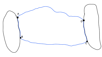
For any and there exist three isometric embeddings of cycles , , in such a way that and have a common path , and have a common path , and have lengths ; the ratio of the length of or to that of or is . (see Figure 4.1).
Proof.
Take in a cyclically irreducible relation , such that is not a consequence of shorter relations of (since is not finitely presented, there are infinitely many such ). Consider in a path starting at an arbitrary vertex and having labelling . This is a cycle with length , assume it is not an isometric embedding. Then some two vertices and are connected with a path such that has fewer edges than both parts of between and . If we keep one of these parts and replace another one by , we obtain two relations in that are shorter than and imply . This contradiction implies the first claim.
To prove the second part of the lemma, it is sufficient to take an isometric embedding of a long cycle, choose another, much longer isometrically embedded cycle that has a long common word with the first one, and finally take a third, long but much shorter than the second one isometrically embedded cycle which has a long almost antipodal common subword with the second one.
More precisely, we argue as follows. For a word in the alphabet we denote by its length. From we know that there exists an infinite sequence of words in the alphabet such that and for any and any , the path in , starting at and labelled is an isometric image of a cycle of length .
Any word of length greater than can be decomposed as follows:
where and . In other words, we chose this decomposition in such a way that two segments labeled by and are almost opposite in the cycle labeled by .
Since the number of such pairs is bounded by , there exist and such that , , and .
In there are vertices and six paths (lower indices denote starting and ending points) , , , , , with label words , , , , , correspondingly (see Figure 4.1).
The cycles , and have labels , and a cyclic shift of correspondingly, they are isometrically embedded, and are geodesics, and all the required inequalities hold. ∎
Theorem 4.8.
Let be a finitely generated group. Then if and only if is virtually free.
Proof.
We know that free groups have , see Remark 3.6. In fact, if the number of generators is at least (see Lemma 4.1), and is otherwise (if is ). Since is a quasi-isometric invariant of groups (see Lemma 2.13), we can conclude that any virtually free group satisfies .
Now we have to prove the non-trivial claim of the theorem. That is, to prove that if is not virtually free and is a finite generating set, then for any order it holds that .
The second claim of Corollary 4.6 says that if is finitely presented but not virtually free, then for any order .
Therefore, it is enough to assume now that is not finitely presented. In this case we consider a mapping of the “trimino figure”, guaranteed by Lemma 4.7, and search for an appropriate snake in the image of this figure. (If we would have a quasi-isometric embedding of a domino figure, with length of its edges large enough, in our group then we could use directly a discrete version of the domino Lemma 3.19. Since we do not have this information, it is more convenient for us to work with the trimino figure).
Suppose that the claim we want to prove is not satisfied: is a group which is not finitely presented, is a finite generating set, is an order on and there are no snakes on points with large elongation in , with respect to the order . In particular, this means that for some there are no snakes on points in with width and of diameter greater than or equal to .
Apply the second part of Lemma 4.7 and consider the image of the “trimino figure” satisfying the claim of this lemma for , .
The cycles , and , constructed in this lemma, are isometrically embedded, , , .
Since and are geodesics, the cycles and have length . From the first claim of Lemma 4.2 we know that the cycle contains points such that , , .
We claim that in there is a (not necessarily directed) continuous path from to the vertex such that it does not intersect with the ball .
First observe that the distance between the cycles and is
Hence does not intersect with , so reaching any point of is enough for our purpose. Since the cycle is isometrically embedded, its intersection with is a geodesic segment of length , denote this segment by . It is clear that .
We also observe that can not intersect with both and . Indeed, since the cycle is isometrically embedded, the distance in between the subsets and is equal to . Without loss of the generality we assume that the set does not intersect with . In particular, . Then there is a path from to such that vertices of it belong to . Denote by the path , this path satisfies the property we were looking for.
Consider some points . If and then we claim that , otherwise we find a snake on points with width and diameter greater than . So, all points of the path are between and , and all points of the circle are greater than (in this sentence “between” and “greater” refers to the order ).
But in the same way we can prove that for some point and any point of we have , this leads to a contradiction. ∎
5. Hyperbolic spaces
It is known that -hyperbolic spaces behave nicely with respect to some questions related to the travelling salesman problem. See Krauthgamer and Lee [KrauthgamerLee] who show that under a natural local assumption on such spaces there exists an approximate randomized algorithm for the travelling salesman problem.
The goal of this section is to prove Theorem 5.10, showing that there is a very efficient order on these spaces to solve the universal travelling salesman problem. In contrast with the context of [KrauthgamerLee], the constant in the bound for the order ratio function can not be close to one even in the case of metric trees (unless the tree is homeomorphic to a ray, line or an interval, otherwise it clearly admits an embedded tripod).
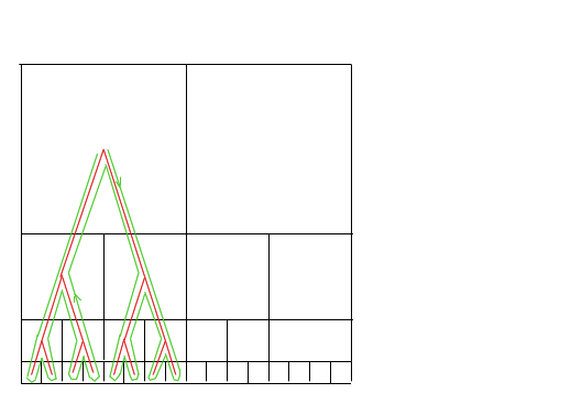
In the introduction it was already mentioned that in view of the theorem of Bonk and Schramm, our main step in the proof of Theorem 5.10 is to prove it for uniformly discrete spaces that are quasi-isometric to hyperbolic spaces . We work with a graph that corresponds to a specific tiling of (also shown on Figure 1.2 for this tiling in the case of ). The order we define on this graph comes from a hierarchical order on a certain associated tree (see Figure 1.2). It is well known that the metric of any finite subset of a -hyperbolic space can be well approximated by the metric of a tree. A comparison lemma (see for example [ghysdelaharpe]) states that given a subset of cardinality in a -hyperbolic space, its metric can be approximated by the metric of a finite tree up to an additive logarithmic error . As we have already mentioned in the introduction, this metric approximation is not enough for our purposes. We will work with some trees, which in some other sense approximate our space, associate an order to these trees and we need check some properties of these trees and their associated orders.
5.1. Definitions and basic properties of -hyperbolic spaces
A metric space is said to be -hyperbolic if there exists such that the following holds. For any points , , , consider three numbers , , . Here we use the notation . We require that the difference between the largest of these three numbers and the middle one is at most . It is well-known that for geodesic metric spaces this definition (with appropriate choice of ) is equivalent to several other possible definitions, one of them is in terms of thin triangles. A geodesic triangle is said to be -slim if each of its sides is contained in the -neighborhood of the union of the two other sides. A geodesic metric space is -hyperbolic if there exists such that any geodesic triangle is -slim. Any Hadamard manifold (complete simply connected Riemannian manifold of sectional curvature ) is -hyperbolic for some depending on (see e.g. Chapter in [ghysdelaharpe]). In particular, a hyperbolic space is -hyperbolic for some . We recall that a quasi-geodesic is the image of an interval with respect to a quasi-isometric embedding. If this quasi-isometry has multiplicative constant and additive constant , we say that such quasi-geodesic is an -quasi-geodesic.
If a metric space is geodesic, a basic property of a -hyperbolic space is that all -quasi-geodesics between points and lie at a bounded distance from any geodesic between , where this distance is estimated in terms of , and . This statement is sometimes called the Morse Lemma.
We also recall that if and are quasi-isometric geodesic metric spaces and is -hyperbolic, then there exists such that is -hyperbolic. For these and other basic properties of -hyperbolic spaces see e.g. [ghysdelaharpe, BridsonHaefliger]. For optimal estimates of the constants in the Morse Lemma see [schur, gouezelschur].
5.2. Binary tiling
There is a well-known tiling of the hyperbolic plane , which is called the binary tiling and also sometimes called the Børøczky tiling. A version of this tiling that we describe below exists in -dimensional hyperbolic spaces ,
Consider the space , the coordinates of this space we denote by . Denote by its half-space with . We will use the words up and down to refer to increases and decreases in the coordinate . We also call changes of this coordinate vertical, and changes of all the other coordinates horizontal. We subdivide (viewed as a subset of Euclidean space into cubes: for integers consider the set of points satisfying
We call such a cube a tile with coordinates , and when we speak about faces of this cube we refer to its -dimensional faces. (This tiling of , that is for and , is shown on Figure 1.2).
We call the subset the layer of the level . The layer of level consists of -dimensional cubes of the same size, with the sides of length . The centers of these cubes form a standard Euclidean -dimensional lattice. A tile with coordinates is adjacent to tiles of the same level with coordinates , it is also adjacent to one of the upper level, namely to and it is adjacent to tiles of the lower level of the form , where each is equal to or .
Consider the graph , the vertices of which correspond to (centers of) tiles, and two vertices are joined by an edge if the tiles are adjacent. We know that the degree of each vertex of is equal to .
We define a metric on the space by putting
We identify together with this metric with the hyperbolic space (half-space model). The distance between two points and is then
Observe that the graph is quasi-isometric to . To see this observe that the mapping from to
is an isometry of , as follows from the above mentioned definition of the hyperbolic metric. Hence any tile can be mapped to any other tile of our tiling by an isometry of . Observe also that each tile has a bounded number of faces, and that each point is adjacent to a bounded number of tiles. Therefore, our graph is quasi-isometric to .
Definition 5.1.
For given two vertices and of the graph we consider a path of the following form. This path makes from several (possibly none) steps upwards to some vertex . After this it makes several horizontal steps to some vertex that is close to : close in the sense that the tiles corresponding to and have a common point. We require that this segment of the path has minimal length among all horizontal paths connecting and in . After that the geodesic makes several steps (possibly none) downwards from to . We will call paths of the form described above up-and-down paths. The first group of edges of the path is called its upwards component, the last group of edges is called its downwards component. We call an up-and-down path which has a minimal number of vertical edges a standard up-and-down path.
Such standard up-and-down paths are essentially unique, that is, their “upwards” and “downwards” components are uniquely defined, and the only freedom is the choice of at most horizontal steps.
Lemma 5.2 (Standard quasi-geodesics).
There exist , depending on the dimension , such that for any two vertices and of the graph a standard up-and-down path between them is an -quasi-geodesic in .
Proof.
Observe that a subpath of an up-and-down path is also an up-and-down path, and that this subpath is clearly standard if the initial one is standard. Therefore in order to show that standard up-and-down paths are quasi-geodesics, it is sufficient to show that for all and in , such paths between and have length at most , where is the distance between and and depends only on .
Observe that a standard quasi-geodesics between two points can be obtained in the following way: given two points and , if the level of is greater than or equal than that of , we first move from upwards to some point of the same level as . Then we start moving upwards (simultaneously) from and until we reach for the first time the points of the same level that are close in the sense described in the definition of up-and-down paths, see Figure 5.1.
Let be the shortest length of a path among paths that move only horizontally from to . Observe that the length of a standard up-and-down path between and is at most . The length of a standard up-and-down path connecting and is clearly the difference of their levels . This shows that, for some positive depending on , the length of a standard up-and-down path between and in is at most .
On the other hand, for any path between and in , observe that its length satisfies . From the distance formula of the half-space model we have
where depends only on . Since and are quasi-isometric, we also conclude that for some depending only on . Hence the length of our up-and-down path is . ∎
We will also call standard up-and-down paths up-and-down quasi-geodesics and standard quasi-geodesics.
If we relax the closeness condition in the definition of up-and-down paths by saying that and are of the same vertical level and at bounded distance (the bound depends on ), one can moreover show that a geodesic between any two points in can be chosen in this standard form. We do not use this statement in our paper, but we mention that it can lead to an alternative proof of Lemma 5.2. We are grateful for the referee for indicating us that such proof is somehow analogous to Lemma 3.10 in [manning].
Let us say that an edge in is vertical if this edge has a non-zero change of coordinate. Now consider a graph which has the same vertex set as and where the edges consist of just the vertical edges of . We denote this graph by .
Remark 5.3.
The graph is a forest. Indeed, observe that any point has only one vertical ascendant, hence this graph does not have cycles. This forest consists of disjoint trees. For example, in the case , these two trees correspond to the two quadrants , and , in the upper half plane .
Denote by one of the connected components of . We know that is a tree. We can introduce an orientation on the edges of , saying that the edges are oriented downwards.
Remark 5.4.
Any finite set of vertices of can be moved to the component by an isometry of .
By Lemma 2.16 if we want to find an order on with bounded order ratio function, it is sufficient to find an order with this property on the connected component . We will check this claim for orders on with convex branches.
In this section when we discuss branches of we mean branches in the sense of an oriented tree: a branch of corresponds to the set of tiles belonging to
| (1) |
for some choice of integers and .
Observe that Lemma 2.18 implies that admits orders such that branches are convex with respect to . We also described explicitly such an order for a finite tree in the beginning of Subsection 3.1, this construction can easily be modified for the infinite tree .
Now we prove
Lemma 5.5.
[Standard paths are inside branches] Suppose that and belong to some branch of the tree . Then the vertices of any standard up-and-down path between and also belong to this branch.
Proof.
Let be a vertex of such that and belong to the branch of . Let
be the shortest path connecting and and let
be the shortest path connecting and . If one of these paths contains the other, the statement of the Lemma is clear.
Otherwise there exists a maximal index such that but the tiles corresponding to and have a common point. For any standard up-and-down path connecting and its upwards component is and its downwards component is . Consider arbitrary vertex of its horizontal component. Any of its coordinates is equal to the corresponding coordinate of or , and from formula 1 it follows that also belongs to the branch of . The Lemma follows. ∎
Lemma 5.6 (Multiplicity upper bound on paths with respect to hierarchical orders).
Let be an order on such that all the branches of the tree are convex with respect to . Consider distinct vertices and for each assume that the sequence of tiles
with and is a standard up-and-down quasi-geodesic, we denote it by . Then each vertical edge appears at most once among upwards edges of the above mentioned paths and at most once among downwards edges. There exists depending only on such that any vertex belongs to at most paths among .
Proof.
Let be some edge in , with one level lower than . Suppose that this edge belongs to the upward part of the standard up-and-down path between and . Take and let us show that can not belong to .
Indeed, belongs to the branch of . We know that the level of is higher than that of , and hence does not belong to the branch of . We can therefore conclude by Lemma 5.5 that is also not inside the branch of . Since branches of the tree are convex with respect to our order, this implies that for any the vertex does not belong to the branch of (since by assumption of the lemma is between and , and since we know that is in the branch, and is not in the branch). This implies that any path going upward from does not enter this branch. In particular, the edge is not on the standard up-and-down path from to . The case of downwards paths is analogous.
Now to prove the last claim of the lemma observe that it is sufficient to bound the multiplicity of all (not necessarily vertical) edges on our path. (Indeed, any but the very last vertex of our path belongs to an edge of our path starting from this vertex).
Consider a horizontal edge . Observe that each standard up-and-down quasi-geodesic that contains is either short, i.e. has length , or long and contains a vertical edge at distance from . The total number of possible short paths that contain is bounded. The number of long paths among that contain is bounded by the doubled number of vertical edges at distance from . ∎
Take a subset in and a point . Let us call a cone the union of all geodesics between and , where the union is taken over all . We denote this cone by . This definition can be also given for an arbitrary metric space if we consider the union of all geodesics between and , but we will use this notion only for .
For a set we denote by its -neighborhood. The standard volume in the space is denoted by , the volume of a ball of radius is denoted by . Clearly, this volume does not depend on the center of the ball, and in the notation above we write without introducing the notation for the center.
Lemma 5.7 (Linear bound for the volume of neighborhoods of a cone).
For all there exists , depending on and , such that if is a curve of length and is a point of , then the volume of the -neighborhood of the cone satisfies .
Proof.
Note that adding a geodesic interval to our curve, we obtain a closed curve of length at most . Therefore we can assume that our curve in the assumption of the lemma is closed.
If we move the point a small distance away from and replace by another curve that is close to in the sense of the Hausdorff metric, then the original cone is contained in a small neighbourhood of the new one. Therefore we can also assume that is at distance from but . We also assume that is a union of geodesics. Further we will use the estimation .
In the sequel we use the following notation. Given a continuous path , its length is denoted by . Given a metric space and , we will use the notation
that is is the minimal cardinality of a -net of .
Observe that for we have
| (2) |
The volume depends clearly only on and . Therefore, it is sufficient to prove a linear upper bound for .
For a piecewise geodesic curve , (with geodesic for all ) and , define the angular length of with respect to as
Decompose the curve into pieces in such a way that and for .
It is clear that is the union of cones . Let us show that for some , depending on and , we have
| (3) |
and for
| (4) |
Moreover, we will show that the -nets that assure the inequalities above can be chosen among -nets containing . This would imply the claim of the lemma, because the union of these -nets is an -net for , and we have the estimation
| (5) |
The term corresponds to the point which belongs to each of our -nets.
Now we will prove our statement for , we assume that it decomposes as a piecewise geodesic . The cone is a union of triangles. In the hyperbolic plane consider a polygon (possibly degenerate) consisting of the same triangles: is such that the triangle is isometric to the triangle for all . (Such is what is called a net, not to be confused with -nets). The perimeter of can be estimated by . For all observe that , this implies that the union of and forms a geodesic, and hence , and therefore, the perimeter of is at most .
By a linear isoperimetric inequality in (see e. g. [teufel] for a more general version), we know that a loop , of length , in a hyperbolic plane of constant curvature is the boundary of a figure of volume (area in ) at most .
Denote by the set of points of that are at distance greater than or equal to from its boundary. Consider an -net of (such a net exists by Remark 2.6). Its cardinality is at most , where is the volume (the area in ) of a ball of radius . We can also find an -net of the boundary of such that and . Observe that is an -net of .
We get therefore an -net of of cardinality at most points (including ). To show that there exists an -net of of the same cardinality, observe the following. The polygon is obtained by unfolding cone of piecewise geodesic curve of angular length at most , then maps to this cone by a map that does not increase distances. Assuming the estimations on , we have proved inequalities 3 and 4 for
| (6) |
| (7) |
∎
In the claim of the Lemma below the word “convex” refers to adding paths between two points, not to Definition 2.17 of convexity with respect to an order. Note that in contrast to the result of [benjaminironen] the number of points (on our path) is not bounded. Given a set in a metric space , define its partial convex hull as the union of all geodesics between pairs of points in .
Lemma 5.8 (Bound on the partial convex hull).
There exists , depending on and , such that if is a curve of length , then the volume of the -neighborhood of its partial convex hull satisfies .
Proof.
Fix some point . Observe that by -hyperbolicity of we know that lies in the -neighborhood of the cone , for some . Therefore, its -neighborhood belongs to the -neighborhood of the cone, and the claim follows therefore from the previous lemma. ∎
Proposition 5.9.
There exists a constant depending on such that for any order on , with branches of all trees of convex with respect to , we have , for any .
Proof.
For any finite subset of we can choose a hierarchical order of and find a subset that is isometric to and that is ordered in the same way as . So we assume that we have a finite subset , of cardinality , and assume that this subset admits a path of length in visiting its points. Let us number the points of the set with respect to an order on , satisfying the assumption of the proposition: . We want to show that
for some constant depending only on .
Connect with , by a geodesic in , and consider the union of these geodesics. We estimate the total number of vertices on the obtained path using Lemma 5.7 about cones and its corollary (Lemma 5.8) to partial convex hulls.
Now for each consider a standard up-and-down path between and :
From Lemma 5.2 we know that these paths are quasi-geodesics in with some constants . Hence they are also quasi-geodesics in with some constants and (depending only on ).
As we have already mentioned, the Morse Lemma for -hyperbolic spaces implies that there exists depending on and (and the hyperbolicity constant of the space ) such that any -quasi-geodesic between two points in belongs to the -neighborhood of any geodesic between these points, see e.g. Chapter 5 of [ghysdelaharpe]. As we have mentioned, , and therefore also depend only on .
Recall that we are discussing a finite set , which admits a path of length in visiting all its points. Since the vertices of form a uniformly discrete space, quasi-isometrically embedded in , there is a piecewise geodesic path of length at most in , visiting all points of . Here the constant depend only on . The constants that we will choose later in the proof will also depend only on .
The geodesics joining points and in lie in . All tiles corresponding to are in the -neighborhood of , for some . Constant can be chosen as the sum of and the diameter of a tile.
We can therefore apply Lemma 5.8 for and and find a constant depending only on such that all tiles containing corresponding points belong to a subset of volume at most of .
Let be the volume of a tile in (since the tiles are isometric they have the same volume). We can conclude that the number of distinct vertices in in the union of quasi-geodesics is at most .
The observation above holds for any order, we did not use that branches are convex with respect to . However, in the following observation this assumption for is essential. We recall that by Lemma 5.6 there exists a constant such that any point appears at most times among the vertices of the quasi-geodesics . This implies that is at most .
∎
As we have already mentioned, the result of Bonk and Schramm [bonkschramm] implies that any -hyperbolic metric space of bounded growth embeds quasi-isometrically into for some . We do not explain the definition of bounded growth but recall that any graph of bounded degree is a particular case of this definition.
Observe that if a space embeds quasi-isometrically into , this space also embeds quasi-isometrically into . Therefore, combining Proposition 5.9 with Lemma 2.8 we obtain
Theorem 5.10.
Let be a -hyperbolic graph of bounded degree. Then there exists an order and a constant such that for all
In the formulation of the Theorem above we use the convention that edges of the graph are of length , and we can assume that they are included in the metric space , see Lemma 3.17.
Remark 5.11.
The order breakpoint of and the constant in Theorem 5.10 of tend to infinity as tends to infinity. To see this it is enough to consider uniform embeddings of a cube of dimension into . For more on this see Section in [ErschlerMitrofanov2].
From Lemma 2.13 it follows that the same claim is clearly true for any uniformly discrete metric space, quasi-isometric to . We remind the reader that for each there exist finitely generated groups quasi-isometric to [Borel63, gromovpiatetski], but it seems to be a challenging open problem [gromovMarkov] to understand whether one can find more elementary constructions of such groups (for ).
Remark 5.12.
The properties of the function we consider are not to be confused with the “travelling salesman property” of a very different nature, introduced for finitely generated groups by Akhmedov [akhmedov1], see also [akhmedov2], [guba]. While hyperbolic groups (and spaces) are best possible cases for our question about , hyperbolic groups are among worst possible case (“TS” groups) for the question of Akhmedov, see [akhmedov1]. We also mention that all amenable groups are not so bad for that problem (they are not “TS” groups, see [guba] , where this observation is attributed to Thurston), while for the questions of our paper there is no visible relation with amenability. Both amenable and non-amenable groups can have finite -dimension (and thus satisfy logarithmic bound for , as we will show in [ErschlerMitrofanov2], see Theorem I) and there are numerous classes of amenable groups satisfying ( [ErschlerMitrofanov2], Corollary 6.8).
5.3. Further examples with bounded order ratio functions
A metric space with bounded order ratio function does not need to be hyperbolic. We have seen already in Section (see Lemma 3.12 and Remark 3.10) that for cactus graphs the order ratio function is bounded. Choosing circles of unbounded length we clearly can obtain not-hyperbolic examples (in particular among graphs of bounded degree).
A wider family of examples is provided by the following lemma.
Lemma 5.13.
Let be a metric space that admits an order such that for all . Let be a subset of . Given , denote by a space which is obtained from copies of by gluing them over . For any the space admits an order such that .
Proof.
For we denote by the subset of that corresponds to the -th copy of . It is clear that is the intersection of all . We define the order on as follows:
-
(1)
if , , then ;
-
(2)
if , then we define if and only if ;
-
(3)
if , , and , then ;
-
(4)
if for some and , then .
Consider a finite set and denote by the length of the shortest path in . We want to estimate from above. Let be the intersection and let for be the intersection . Without loss of generality we assume that all are non empty.
It is clear that
where is the distance between the maximal point of with respect to and the minimal point of with respect to .
For any we can estimate , , . Hence . ∎
We know that the assumption of Lemma 5.13 is in particular satisfied when is a uniformly discrete hyperbolic space of uniformly bounded growth. This assumption holds also for any metric tree (not necessarily uniformly discrete). Figure 5.2 shows an example of the construction above, where is a tree, . Observe that the space in this example is non-hyperbolic. For all it contains an isometric copy of a cycle of length .
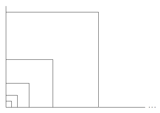
Other particular cases of the spaces from the claim of Lemma 5.13 are spaces obtained by gluing together several copies of graphs (which is quasi-isometric to ), by a horizontal subspace in the half-space model of dimension . We recall that in our terminology is defined to be the equivalence class, with respect to equivalence up to a multiplicative constant, of functions , where is some -net of . If we glue two copies of by this horizontal subspace, we obtain a space , satisfying , but admitting contractible quasi-isometrically embedded circles of arbitrarily large length.
We have discussed non-hyperbolic spaces with bounded function . It seems interesting to understand whether this can happen for finitely generated non-hyperbolic groups. In this context we ask the following questions: what is the asymptotics of for solvable Baumslag-Solitar groups? The same question can be asked for .
Appendix A Proof of Lemma 3.17
Let be a graph (finite or infinite) with edges of length 1 and let be an order on the set of its vertices. We remind the reader that is the order defined on (including its edges) described in Definition 3.16.
We want to prove that for all it holds that
In the definition of the order we consider the partition of into star figures. Consider a subset . First observe that if belongs to one of the stars, then . This is because the order on this star is (a very particularly easy) example of a hierarchical order on a tree. Also observe that if belongs to one of the edges of the graph, then . Indeed, the edge consists of two halves, in each of the halves the points are visited in a linear order, and the jump from one half to the other is not larger than the diameter of the set. In the sequel we can therefore assume that does not belong to one of the star figures and also is not inside one of the edges of the graph.
Assume that . The points of belong to star figures. Denote by the set of centers of these stars, and put . It is clear that . We recall that by definition of our order the path first visits all points of one of the star figures, then all points from another one and so on. We can therefore write
where is the sum of lengths of jumps between distinct star figures (the number of such jumps is ), and is the total length of jumps inside star figures.
First we estimate . The length of the jump from the star figure centered at to the star figure centered at is at most . This implies that the total sum of such jumps is not greater than the length of the associated path in , that is
Let us understand the relation between and . If we have some path through the points of , we can modify it to visit also all points of : after the first visit of each star figure, except of the first and last visited star figures, we jump to its center and back after this first visit. In the first visited star figure, we start with its center and then continue as in the original path. In the last visited star figure, after the last visit we jump to its center (and do not jump back).
The length is increased by at most for each star figure, and not by more than in case of the first visited star figure and the last visited star figure. Therefore,
For the optimal path of consider for each visited star figure (except the first one) the first visited point. These points are distinct middle points of some edges. Since the distance between two distinct middle points is at least , we observe that
Summing this with the inequality (which holds because of our assumption that is not inside one star figure and not inside one edge), we get that . And, therefore, satisfies .
Now we estimate . Let us look at the position of the points of on the corresponding edges of the graph. Suppose that belongs to the edge . We denote by the middle point of this edge, and suppose that belongs to the half-edge , . We suppose also that the interval does not have other points of . In this case we associate to the number . In other words, we associate the distance from to the vertex if is the most distant point from the vertex on the half-edge . Otherwise, we do not associate anything to . Observe that if is the total sum of associated numbers, then because of the hierarchical order on each star figure. Note that for each edge there are at most two associated numbers. Let us call a point of leading if it has an associated number and it is the largest of the two numbers associated to the points of its edge. The set of leading points is denoted by . The sum of the numbers associated to leading points clearly satisfies . If we have a leading point with an associated number , and another leading point with an associated number , then the distance between these two points is at least . Taking in account that does not belong to one edge and hence , we get , and consequently, . Therefore,
this concludes the proof of Lemma 3.17. ∎
Appendix B A theorem of Kapovich about tripods in geodesic metric spaces and related questions
Definition B.1.
Let be a metric space. An -tripod is the union of an -geodesic (a curve of length at most ) and a curve of length at most , where is the distance from to , where .
We do not recall the definition of path metric spaces (a generalisation of a notion of geodesic metric spaces, which makes sense for spaces which are not necessarily complete), but mention that any geodesic metric space is an example of a path metric space.
We use the following result of M. Kapovich.
Claim B.2.
[[kapovich], Theorem 1.4, see also Corollary 7.3] Let be a path metric space not quasi-isometric to a point, a ray or a line. Then for any and any , admits an -tripod.
Moreover, Kapovich showed that for any one can find a -tripod inside any ultralimit of the constant sequence of (pointed) metric spaces from the theorem. Since for proper geodesic metric spaces, such metric spaces (if not quasi-isometric to a point a ray or a line) admit tripods with being a geodesic segment and being a geodesic segment of shortest length to .
Now we recall our notation for tripods: a tripod consists of segments of length glued together by an endpoint.
Claim B.3.
Let be a geodesic metric space and let be a tripod with center and legs , and . Let be a mapping and denote , , , . Assume that is a length parametrized curve such that
for . Assume that is a length parametrized geodesic curve, and , where is the distance from to .
Then the map satisfies
for any .
Proof.
It is clear that for any that correspond to the leg we have . We also know that for any such that (that is, in the union of two legs) it holds that
It is sufficient therefore to consider the case when the point and the other point .
Observe that in this case
and hence
Denote by and denote by . It is clear that .
If , then and
If , then and
∎
Using Claim B.2 (taking in account a remark below this claim) and Claim B.3 we conclude that if is a geodesic metric space, not quasi-isometric to a point, a ray or a line, then for any and each there exists such that for any
Thus we have proved Lemma 4.3.
Remark B.4.
It is clear that the constant in Claim B.3 can not be improved, as an example of a circle shows (or, if one wants to avoid degenerate tripods, an example of an interval attached by its endpoint to a circle)
References
- [1] AkhmedovAzerTravelling salesman problem in groupstitle={Geometric methods in group theory}, series={Contemp. Math.}, volume={372}, publisher={Amer. Math. Soc., Providence, RI}, 2005225–230Review MathReviewsDocument@article{akhmedov1, author = {Akhmedov, Azer}, title = {Travelling salesman problem in groups}, conference = {title={Geometric methods in group theory}, }, book = {series={Contemp. Math.}, volume={372}, publisher={Amer. Math. Soc., Providence, RI}, }, date = {2005}, pages = {225–230}, review = {\MR{2140092}}, doi = {10.1090/conm/372/06888}}
- [3] AkhmedovAzerPerturbation of wreath products and quasi-isometric rigidity. iInt. Math. Res. Not. IMRN20084Art. ID rnn004, 18ISSN 1073-7928Review MathReviewsDocument@article{akhmedov2, author = {Akhmedov, Azer}, title = {Perturbation of wreath products and quasi-isometric rigidity. I}, journal = {Int. Math. Res. Not. IMRN}, date = {2008}, number = {4}, pages = {Art. ID rnn004, 18}, issn = {1073-7928}, review = {\MR{2424177}}, doi = {10.1093/imrn/rnn004}}
- [5] BenjaminiItaiEldanRonenConvex hulls in the hyperbolic spaceGeom. Dedicata1602012365–371ISSN 0046-5755Review MathReviewsDocument@article{benjaminironen, author = {Benjamini, Itai}, author = {Eldan, Ronen}, title = {Convex hulls in the hyperbolic space}, journal = {Geom. Dedicata}, volume = {160}, date = {2012}, pages = {365–371}, issn = {0046-5755}, review = {\MR{2970060}}, doi = {10.1007/s10711-011-9687-8}}
- [7] BartholdiIIIJ. J.PlatzmanL. K.An planar travelling salesman heuristic based on spacefilling curvesOper. Res. Lett.119824121–125ISSN 0167-6377Review MathReviewsDocument@article{bartholdiplatzman82, author = {Bartholdi, J. J., III}, author = {Platzman, L. K.}, title = {An $O(N\,{\rm log}\,N)$ planar travelling salesman heuristic based on spacefilling curves}, journal = {Oper. Res. Lett.}, volume = {1}, date = {1982}, number = {4}, pages = {121–125}, issn = {0167-6377}, review = {\MR{687352}}, doi = {10.1016/0167-6377(82)90012-8}}
- [9] PlatzmanLoren K.BartholdiIIIJohn J.Spacefilling curves and the planar travelling salesman problemJ. Assoc. Comput. Mach.3619894719–737ISSN 0004-5411Review MathReviewsDocument@article{bartholdiplatzman89, author = {Platzman, Loren K.}, author = {Bartholdi, John J., III}, title = {Spacefilling curves and the planar travelling salesman problem}, journal = {J. Assoc. Comput. Mach.}, volume = {36}, date = {1989}, number = {4}, pages = {719–737}, issn = {0004-5411}, review = {\MR{1072243}}, doi = {10.1145/76359.76361}}
- [11] BertsimasDimitrisGrigniMichelangeloWorst-case examples for the spacefilling curve heuristic for the euclidean traveling salesman problemOper. Res. Lett.819895241–244ISSN 0167-6377Review MathReviewsDocument@article{bertsimasgrigni, author = {Bertsimas, Dimitris}, author = {Grigni, Michelangelo}, title = {Worst-case examples for the spacefilling curve heuristic for the Euclidean traveling salesman problem}, journal = {Oper. Res. Lett.}, volume = {8}, date = {1989}, number = {5}, pages = {241–244}, issn = {0167-6377}, review = {\MR{1022839}}, doi = {10.1016/0167-6377(89)90047-3}}
- [13] BhalgatAnandChakrabartyDeeparnabKhannaSanjeevOptimal lower bounds for universal and differentially private steiner trees and tspstitle={Approximation, randomization, and combinatorial optimization}, series={Lecture Notes in Comput. Sci.}, volume={6845}, publisher={Springer, Heidelberg}, 201175–86Review MathReviews@article{bhalgatetal, author = {Bhalgat, Anand}, author = {Chakrabarty, Deeparnab}, author = {Khanna, Sanjeev}, title = {Optimal lower bounds for universal and differentially private Steiner trees and TSPs}, conference = {title={Approximation, randomization, and combinatorial optimization}, }, book = {series={Lecture Notes in Comput. Sci.}, volume={6845}, publisher={Springer, Heidelberg}, }, date = {2011}, pages = {75–86}, review = {\MR{2863250}}}
- [15] BonkM.SchrammO.Embeddings of gromov hyperbolic spacesGeom. Funct. Anal.1020002266–306ISSN 1016-443XReview MathReviewsDocument@article{bonkschramm, author = {Bonk, M.}, author = {Schramm, O.}, title = {Embeddings of Gromov hyperbolic spaces}, journal = {Geom. Funct. Anal.}, volume = {10}, date = {2000}, number = {2}, pages = {266–306}, issn = {1016-443X}, review = {\MR{1771428}}, doi = {10.1007/s000390050009}}
- [17] BorelArmandCompact clifford-klein forms of symmetric spacesTopology21963111–122ISSN 0040-9383Review MathReviewsDocument@article{Borel63, author = {Borel, Armand}, title = {Compact Clifford-Klein forms of symmetric spaces}, journal = {Topology}, volume = {2}, date = {1963}, pages = {111–122}, issn = {0040-9383}, review = {\MR{0146301}}, doi = {10.1016/0040-9383(63)90026-0}}
- [19] BridsonMartin R.HaefligerAndréMetric spaces of non-positive curvatureGrundlehren der Mathematischen Wissenschaften [Fundamental Principles of Mathematical Sciences]319Springer-Verlag, Berlin1999xxii+643ISBN 3-540-64324-9Review MathReviewsDocument@book{BridsonHaefliger, author = {Bridson, Martin R.}, author = {Haefliger, Andr\'{e}}, title = {Metric spaces of non-positive curvature}, series = {Grundlehren der Mathematischen Wissenschaften [Fundamental Principles of Mathematical Sciences]}, volume = {319}, publisher = {Springer-Verlag, Berlin}, date = {1999}, pages = {xxii+643}, isbn = {3-540-64324-9}, review = {\MR{1744486}}, doi = {10.1007/978-3-662-12494-9}}
- [21] ChristodoulouGeorgeSgouritsaAlkminiAn improved upper bound for the universal tsp on the gridtitle={Proceedings of the Twenty-Eighth Annual ACM-SIAM Symposium on Discrete Algorithms}, publisher={SIAM, Philadelphia, PA}, 20171006–1021Review MathReviewsDocument@article{Christodoulou, author = {Christodoulou, George}, author = {Sgouritsa, Alkmini}, title = {An improved upper bound for the universal TSP on the grid}, conference = {title={Proceedings of the Twenty-Eighth Annual ACM-SIAM Symposium on Discrete Algorithms}, }, book = {publisher={SIAM, Philadelphia, PA}, }, date = {2017}, pages = {1006–1021}, review = {\MR{3627793}}, doi = {10.1137/1.9781611974782.64}}
- [23] DruţuCorneliaKapovichMichaelGeometric group theoryAmerican Mathematical Society Colloquium Publications63With an appendix by Bogdan NicaAmerican Mathematical Society, Providence, RI2018xx+819ISBN 978-1-4704-1104-6Review MathReviews@book{drutukapovichbook, author = {Dru\c{t}u, Cornelia}, author = {Kapovich, Michael}, title = {Geometric group theory}, series = {American Mathematical Society Colloquium Publications}, volume = {63}, note = {With an appendix by Bogdan Nica}, publisher = {American Mathematical Society, Providence, RI}, date = {2018}, pages = {xx+819}, isbn = {978-1-4704-1104-6}, review = {\MR{3753580}}}
- [25] DunwoodyM. J.The accessibility of finitely presented groupsInvent. Math.8119853449–457ISSN 0020-9910Review MathReviewsDocument@article{dunwoody, author = {Dunwoody, M. J.}, title = {The accessibility of finitely presented groups}, journal = {Invent. Math.}, volume = {81}, date = {1985}, number = {3}, pages = {449–457}, issn = {0020-9910}, review = {\MR{807066}}, doi = {10.1007/BF01388581}}
- [27] EadesPatrickMestreJuliánAn optimal lower bound for hierarchical universal solutions for tsp on the planeComputing and combinatorics. 26th international conference, COCOON 2020, Atlanta, GA, USA, August 29–31, 2020. Proceedings222–2332020Cham: Springer@article{eades2, author = {Eades, Patrick}, author = {Mestre, Juli\'{a}n}, title = {An optimal lower bound for hierarchical universal solutions for TSP on the plane}, journal = {Computing and combinatorics. 26th international conference, COCOON 2020, Atlanta, GA, USA, August 29–31, 2020. Proceedings}, pages = {222–233}, date = {2020}, publisher = {Cham: Springer}}
- [29] ErschlerAnnaMitrofanovIvanAssouad-nagata dimension and gap for ordered metric spacesto appear in Commenarii Mathematici Helvetici, https://arxiv.org/abs/2109.12181@article{ErschlerMitrofanov2, author = {Erschler, Anna}, author = {Mitrofanov, Ivan}, title = {Assouad-Nagata dimension and gap for ordered metric spaces}, status = {to appear in Commenarii Mathematici Helvetici, https://arxiv.org/abs/2109.12181}}
- [31] Sur les groupes hyperboliques d’après mikhael gromovFrenchProgress in Mathematics83GhysÉ.de la HarpeP.Papers from the Swiss Seminar on Hyperbolic Groups held in Bern, 1988Birkhäuser Boston Inc.Boston, MA1990xii+285ISBN 0-8176-3508-4Review MathReviews@collection{ghysdelaharpe, title = {Sur les groupes hyperboliques d'apr\`es Mikhael Gromov}, language = {French}, series = {Progress in Mathematics}, volume = {83}, editor = {Ghys, {\'E}.}, editor = {de la Harpe, P.}, note = {Papers from the Swiss Seminar on Hyperbolic Groups held in Bern, 1988}, publisher = {Birkh\"auser Boston Inc.}, place = {Boston, MA}, date = {1990}, pages = {xii+285}, isbn = {0-8176-3508-4}, review = {\MR{1086648 (92f:53050)}}}
- [33] GorodezkyIgorKleinbergRobert D.ShmoysDavid B.SpencerGwenImproved lower bounds for the universal and a priori tsptitle={Approximation, randomization, and combinatorial optimization}, series={Lecture Notes in Comput. Sci.}, volume={6302}, publisher={Springer, Berlin}, 2010178–191Review MathReviews@article{gorodezkyetal, author = {Gorodezky, Igor}, author = {Kleinberg, Robert D.}, author = {Shmoys, David B.}, author = {Spencer, Gwen}, title = {Improved lower bounds for the universal and {\it a prior}i TSP}, conference = {title={Approximation, randomization, and combinatorial optimization}, }, book = {series={Lecture Notes in Comput. Sci.}, volume={6302}, publisher={Springer, Berlin}, }, date = {2010}, pages = {178–191}, review = {\MR{2755835}}}
- [35] GouëzelSébastienShchurVladimirA corrected quantitative version of the morse lemmaJ. Funct. Anal.277201941258–1268ISSN 0022-1236Document@article{gouezelschur, author = {Gou\"ezel, S\'ebastien}, author = {Shchur, Vladimir}, title = {A corrected quantitative version of the Morse lemma}, journal = {J. Funct. Anal.}, volume = {277}, date = {2019}, number = {4}, pages = {1258–1268}, issn = {0022-1236}, doi = {https://doi.org/10.1016/j.jfa.2019.02.021}}
- [37] GromovM.Piatetski-ShapiroI.Nonarithmetic groups in lobachevsky spacesInst. Hautes Études Sci. Publ. Math.66198893–103ISSN 0073-8301Review MathReviews@article{gromovpiatetski, author = {Gromov, M.}, author = {Piatetski-Shapiro, I.}, title = {Nonarithmetic groups in Lobachevsky spaces}, journal = {Inst. Hautes \'{E}tudes Sci. Publ. Math.}, number = {66}, date = {1988}, pages = {93–103}, issn = {0073-8301}, review = {\MR{932135}}}
- [39] GromovM.Hyperbolic dynamics, markov partitions and symbolic categories, chapters and preprint 2016, https://www.ihes.fr/ gromov/wp-content/uploads/2018/08/SymbolicDynamicalCategories.pdf
- [41] @article{gromovMarkov, author = {Gromov, M.}, title = {Hyperbolic dynamics, Markov partitions and Symbolic Categories, Chapters $1$ and $2$}, journal = {{preprint 2016, https://www.ihes.fr/~gromov/wp-content/uploads/2018/08/SymbolicDynamicalCategories.pdf} \par}}
- [42] GrovesD.ManningJ.F.Dehn filling in relatively hyperbolic groups. Isr. J. Math.168317–4292008@article{manning, author = {Groves, D.}, author = {Manning, J.F.}, title = {Dehn filling in relatively hyperbolic groups.}, journal = { Isr. J. Math.}, number = {168}, pages = {317–429}, date = {2008}}
- [44] GubaV. S.Traveller salesman property and richard thompson’s group title={Topological and asymptotic aspects of group theory}, series={Contemp. Math.}, volume={394}, publisher={Amer. Math. Soc., Providence, RI}, 2006137–142Review MathReviewsDocument@article{guba, author = {Guba, V. S.}, title = {Traveller salesman property and Richard Thompson's group $F$}, conference = {title={Topological and asymptotic aspects of group theory}, }, book = {series={Contemp. Math.}, volume={394}, publisher={Amer. Math. Soc., Providence, RI}, }, date = {2006}, pages = {137–142}, review = {\MR{2216711}}, doi = {10.1090/conm/394/07439}}
- [46] HajiaghayiMohammad T.KleinbergRobertLeightonTomImproved lower and upper bounds for universal tsp in planar metricstitle={Proceedings of the Seventeenth Annual ACM-SIAM Symposium on Discrete Algorithms}, publisher={ACM, New York}, 2006649–658Review MathReviewsDocument@article{HKL, author = {Hajiaghayi, Mohammad T.}, author = {Kleinberg, Robert}, author = {Leighton, Tom}, title = {Improved lower and upper bounds for universal TSP in planar metrics}, conference = {title={Proceedings of the Seventeenth Annual ACM-SIAM Symposium on Discrete Algorithms}, }, book = {publisher={ACM, New York}, }, date = {2006}, pages = {649–658}, review = {\MR{2368861}}, doi = {10.1145/1109557.1109628}}
- [48] KapovichMichaelTriangle inequalities in path metric spacesGeom. Topol.1120071653–1680ISSN 1465-3060Review MathReviewsDocument@article{kapovich, author = {Kapovich, Michael}, title = {Triangle inequalities in path metric spaces}, journal = {Geom. Topol.}, volume = {11}, date = {2007}, pages = {1653–1680}, issn = {1465-3060}, review = {\MR{2350463}}, doi = {10.2140/gt.2007.11.1653}}
- [50] HodaNimaShortcut graphs and groupsTrans. Amer. Math. Soc.375202242417–2458ISSN 0002-9947Review MathReviewsDocument@article{Nima, author = {Hoda, Nima}, title = {Shortcut graphs and groups}, journal = {Trans. Amer. Math. Soc.}, volume = {375}, date = {2022}, number = {4}, pages = {2417–2458}, issn = {0002-9947}, review = {\MR{4391723}}, doi = {10.1090/tran/8555}}
- [52] JiaLujunLinGuolongNoubirGuevaraRajaramanRajmohanSundaramRaviUniversal approximations for tsp, steiner tree, and set covertitle={STOC'05: Proceedings of the 37th Annual ACM Symposium on Theory of Computing}, publisher={ACM, New York}, 2005386–395Review MathReviewsDocument@article{jiadoubling, author = {Jia, Lujun}, author = {Lin, Guolong}, author = {Noubir, Guevara}, author = {Rajaraman, Rajmohan}, author = {Sundaram, Ravi}, title = {Universal approximations for TSP, Steiner tree, and set cover}, conference = {title={STOC'05: Proceedings of the 37th Annual ACM Symposium on Theory of Computing}, }, book = {publisher={ACM, New York}, }, date = {2005}, pages = {386–395}, review = {\MR{2181640}}, doi = {10.1145/1060590.1060649}}
- [54] JustinJacquesGroupes et semi-groupes à croissance linéaireFrenchC. R. Acad. Sci. Paris Sér. A-B2731971A212–A214ISSN 0151-0509Review MathReviews@article{justin71, author = {Justin, Jacques}, title = {Groupes et semi-groupes \`a croissance lin\'{e}aire}, language = {French}, journal = {C.~R.~Acad. Sci. Paris S\'{e}r. A-B}, volume = {273}, date = {1971}, pages = {A212–A214}, issn = {0151-0509}, review = {\MR{289689}}}
- [56] KrauthgamerRobertLeeJamesAlgorithms on negatively curved spaces47th Annual IEEE Symposium on Foundation of Computer Science (FOCS’06), date=2006, pages=119-132 @article{KrauthgamerLee, author = {Robert Krauthgamer}, author = {James Lee}, title = {Algorithms on negatively curved spaces}, journal = {47th Annual IEEE Symposium on Foundation of Computer Science (FOCS'06), date={2006}, pages={119-132} }}
- [58] MannAvinoamHow groups growLondon Mathematical Society Lecture Note Series395Cambridge University Press, Cambridge2012x+199ISBN 978-1-107-65750-2Review MathReviews@book{MannHowgroupsgrow, author = {Mann, Avinoam}, title = {How groups grow}, series = {London Mathematical Society Lecture Note Series}, volume = {395}, publisher = {Cambridge University Press, Cambridge}, date = {2012}, pages = {x+199}, isbn = {978-1-107-65750-2}, review = {\MR{2894945}}}
- [60] SchalekampFransShmoysDavid B.Algorithms for the universal and a priori tspOper. Res. Lett.36200811–3ISSN 0167-6377Review MathReviewsDocument@article{Schalekamp, author = {Schalekamp, Frans}, author = {Shmoys, David B.}, title = {Algorithms for the universal and a priori TSP}, journal = {Oper. Res. Lett.}, volume = {36}, date = {2008}, number = {1}, pages = {1–3}, issn = {0167-6377}, review = {\MR{2377182}}, doi = {10.1016/j.orl.2007.04.009}}
- [62] ShchurVladimirA quantitative version of the morse lemma and quasi-isometries fixing the ideal boundaryJ. Funct. Anal.26420133815–836ISSN 0022-1236Review MathReviewsDocument@article{schur, author = {Shchur, Vladimir}, title = {A quantitative version of the Morse lemma and quasi-isometries fixing the ideal boundary}, journal = {J. Funct. Anal.}, volume = {264}, date = {2013}, number = {3}, pages = {815–836}, issn = {0022-1236}, review = {\MR{3003738}}, doi = {10.1016/j.jfa.2012.11.014}}
- [64] SerreJean-PierreTreesSpringer Monographs in MathematicsTranslated from the French original by John Stillwell; Corrected 2nd printing of the 1980 English translationSpringer-Verlag, Berlin2003x+142ISBN 3-540-44237-5Review MathReviews@book{serreTrees, author = {Serre, Jean-Pierre}, title = {Trees}, series = {Springer Monographs in Mathematics}, note = {Translated from the French original by John Stillwell; Corrected 2nd printing of the 1980 English translation}, publisher = {Springer-Verlag, Berlin}, date = {2003}, pages = {x+142}, isbn = {3-540-44237-5}, review = {\MR{1954121}}}
- [66] TeufelEberhardA generalization of the isoperimetric inequality in the hyperbolic planeArch. Math. (Basel)5719915508–513ISSN 0003-889XReview MathReviewsDocument@article{teufel, author = {Teufel, Eberhard}, title = {A generalization of the isoperimetric inequality in the hyperbolic plane}, journal = {Arch. Math. (Basel)}, volume = {57}, date = {1991}, number = {5}, pages = {508–513}, issn = {0003-889X}, review = {\MR{1129528}}, doi = {10.1007/BF01246751}}
- [68]