Multi-Iteration Stochastic Optimizers

Abstract.

We here introduce Multi-Iteration Stochastic Optimizers, a novel class of first-order stochastic optimizers where the coefficient of variation of the mean gradient approximation, its relative statistical error, is estimated and controlled using successive control variates along the path of iterations. By exploiting the correlation between iterates, control variates may reduce the estimator’s variance so that an accurate estimation of the mean gradient becomes computationally affordable. We name the estimator of the mean gradient Multi-Iteration stochastiC Estimator—MICE. In principle, MICE can be flexibly coupled with any first-order stochastic optimizer given its non-intrusive nature. Optimally, our generic algorithm decides whether to drop a particular iteration out of the control variates hierarchy, restart it, or clip it somewhere in the hierarchy, discarding previous iterations. We present a simplified study of the convergence and complexity of Multi-Iteration Stochastic Optimizers for strongly-convex and $L$-smooth functions. Motivated by this analysis, we provide a generic step-size choice for Stochastic Gradient Descent (SGD) with MICE, which, combined with the above characteristics, yields an efficient and robust stochastic optimizer. To assess the efficiency of MICE, we present several examples in which we use SGD-MICE and Adam-MICE. We include one example based on a stochastic adaptation of the Rosenbrock function and logistic regression training for various datasets. When compared to SGD, SAG, SAGA, SRVG, and SARAH methods, the Multi-Iteration Stochastic Optimizers reduced, without the need to tune parameters for each example, the gradient sampling cost in all cases tested, also lowering the total runtime in some cases.

AMS subject classifications: $\cdot$ 65K05 $\cdot$ 90C15 $\cdot$ 65C05 $\cdot$
Keywords: Stochastic Optimization; Monte Carlo; Multilevel Monte Carlo; Variance Reduction; Control Variates; Machine Learning

1. Introduction

We focus on the stochastic optimization problem of minimizing the objective function $\mathbb{E}[f(\boldsymbol{\xi},\boldsymbol{\theta})|\boldsymbol{\xi}],$ where $f$ is a given real-valued function, $\boldsymbol{\xi}$ is the design variable vector, $\boldsymbol{\theta}$ is a random vector, and $\mathbb{E}[\cdot|\boldsymbol{\xi}]$ is the expectation conditioned on $\boldsymbol{\xi}$. Stochastic optimization problems [1, 2, 3] are relevant to different fields, such as Machine Learning [4], Stochastic Optimal Control [5, 6], Computational Finance [7, 8, 9], Economics [10], Insurance [11], Communication Networks [12], Queues and Supply Chains [13], and Bayesian Optimal Design of Experiments [14, 15], among many others.

In the same spirit and inspired by the work by Heinrich [16] and Giles [17] on Multilevel Monte Carlo methods, we propose the Multi-Iteration stochastiC Estimator—MICE—to obtain a computationally efficient and affordable approximation of the mean gradient, $\nabla_{\boldsymbol{\xi}}\mathbb{E}[f(\boldsymbol{\xi},\boldsymbol{\theta})|\boldsymbol{\xi}]$, which may be coupled with any first order stochastic optimizer in a non-intrusive fashion. Combining MICE with any stochastic optimizer furnishes Multi-Iteration Stochastic Optimizers, a novel class of efficient and robust stochastic optimizers. In this class of stochastic optimizers, the mean gradient estimator’s relative variance is controlled using successive control variates based on previous iterations’ available information. This procedure results in a more accurate yet affordable estimation of the mean gradient. In approximating the mean gradient, MICE constructs a hierarchy of iterations and performs control variates for every pair of nested elements of this hierarchy. As the stochastic optimization evolves, we increase the number of samples along the hierarchy while keeping the previously sampled gradients, i.e., we use gradient information from previous iterations to reduce the variance in the current gradient estimate, which is a crucial feature to make MICE competitive. We design MICE to achieve a given relative statistical error for the mean gradient with minimum additional gradient sampling cost. Indeed, in the MICE hierarchy constructed along the stochastic optimization path $\{\boldsymbol{\xi}_{\ell}\}_{\ell=0}^{k}$, our generic optimizer optimally decides whether to drop a particular iteration $\ell$ out of the hierarchy or restart it in order to reduce the total optimization work. Moreover, it can decide if it is advantageous, from the computational work perspective, to clip the hierarchy at some point $\ell$, discarding the iterations before $\ell$. Since we control the gradients’ statistical error using an estimate of the gradient norm, we employ a resampling technique to get a gradient norm estimate, reducing the effect of sampling error and resulting in robust optimizers. We note in passing that MICE can be adjusted to the case of finite populations; see Remark 7, for optimization problems arising in supervised machine learning.

Generally speaking, in first-order stochastic optimization algorithms that produce convergent iterates, the mean gradient converges to zero as the number of iterations, $k$, goes to infinity, that is $\left\lVert{\mathbb{E}[\nabla_{\boldsymbol{\xi}}f(\boldsymbol{\xi}_{k},\boldsymbol{\theta})|\boldsymbol{\xi}_{k}]}\right\rVert\to 0$; however, the gradient covariance, $\mathbb{C}[\nabla_{\boldsymbol{\xi}}f(\boldsymbol{\xi}_{k},\boldsymbol{\theta}),\nabla_{\boldsymbol{\xi}}f(\boldsymbol{\xi}_{k},\boldsymbol{\theta})|\boldsymbol{\xi}_{k}]$, does not. Thus, to ensure convergence of the iterates $\boldsymbol{\xi}_{k}$, in the literature it is customary to use decreasing step-size (learning rate) schedules, reducing the effect of the statistical error in the gradient onto the iterates $\boldsymbol{\xi}_{k}$. However, this approach also results in sublinear convergence rates [18]. Another approach to deal with the gradient’s statistical error is to increase the sample sizes (batch sizes) while keeping the step-size fixed, thus avoiding worsening the convergence. Byrd et al. [19] propose to adaptively increase the sample sizes to guarantee that the trace of the covariance matrix of the mean gradient is proportional to its norm. This approach forces the statistical error to decrease as fast as the gradient norm. Balles et al. [20] use a similar approach; however, instead of setting a parameter to control the statistical error, they set a step-size and find the parameter that guarantees the desired convergence. Bollapragada et al. [21] propose yet another approach to control the variance of gradient estimates in stochastic optimization, which they call the inner product test. Their approach ensures that descent directions are generated sufficiently often.

Instead of increasing the sample size, some methods rely on using control variates with respect to previously sampled gradients to reduce the variance in current iterations and thus be able to keep a fixed step-size. Pioneering ideas of control variates in stochastic optimization, by Johnson & Zhang [22], profit on an accurate mean gradient estimation at the initial guess $\boldsymbol{\xi}_{0}$, $\nabla_{\boldsymbol{\xi}}\mathbb{E}[f(\boldsymbol{\xi}_{0},\boldsymbol{\theta})|\boldsymbol{\xi}_{0}]$, to update and compute, via single control variates, an inexpensive and accurate version of the mean gradient at the iteration $k$, $\nabla_{\boldsymbol{\xi}}\mathbb{E}[f(\boldsymbol{\xi}_{k},\boldsymbol{\theta})|\boldsymbol{\xi}_{k}]$. Instead of doing control variates with respect to one starting full-gradient, SARAH, by Nguyen et al. [23], computes an estimate of the gradient at the current iteration by using control variates with respect to the last iteration. An ‘inexact’ version of SARAH is presented in [24], where SARAH is generalized to the minimization of expectations. In the spirit of successive control variates, SPIDER by Fang et al. [25] uses control variates between subsequent iterations; however, it employs the normalized gradient descent instead of plain gradient descent. In a different approach, SAGA, by Defazio et al. [26], keeps in the memory the last gradient $\nabla_{\boldsymbol{\xi}}f$ observed for each data point and computes $\nabla_{\boldsymbol{\xi}}\mathbb{E}[f(\boldsymbol{\xi}_{k},\boldsymbol{\theta})|\boldsymbol{\xi}_{k}]$ using control variates with respect to the average of this memory. Lastly, many algorithms try to ‘adapt’ the initial batch size of the hierarchy of batches using predefined rules, such as exponential or polynomial growth, as presented by Friedlander & Schmidt [27], or based on statistical bounds as discussed by De Soham et al. [28] and Ji et al. [29], to mention a few.

Although Multi-Iteration Stochastic Optimizers share similarities with SVRG [22], SARAH, and SPIDER, our stochastic optimizers distinctly control the relative variance in gradient estimates. We achieve this control by sampling the entire hierarchy of iterations, optimally distributing the samples to minimize the gradient sampling cost. Moreover, we provide additional flexibility by including dropping, restart, and clipping operations in the MICE hierarchy updates.

Since MICE is non-intrusive and designed for both continuous and discrete random variables, it can be coupled with most available optimizers with ease. For instance, we couple MICE with SGD [30] and Adam [31], showing the robustness of our approach. The Adam algorithm by Kingma & Ba [31] does not exploit control variates techniques for variance reduction. Instead, it reduces the gradient estimator’s variance based on iterate history by adaptive estimates of lower-order moments, behaving similarly to a filter. Thus, the coupling Adam-MICE profits from the information available in the optimizer path in more than one way. Finally, the reader is referred to the books by Spall [32] and Shapiro, Dentcheva, and Ruszczyński [33] for comprehensive overviews on stochastic optimization.

To assess MICE’s applicability, we numerically minimize expectations of continuous and discrete random variables using analytical functions and logistic regression datasets, respectively. Also, we compare SGD-MICE with SVRG, SARAH, SAG, and SAGA in training the logistic regression model with datasets with different sizes and numbers of features.

The remainder of this work is as follows. In §2, we construct the MICE statistical estimator §2.1; define its statistical error §2.2; compute the optimal number of samples for the current hierarchy §2.3; present and derive the criteria for dropping iterations out of the hierarchy §2.4, restarting the hierarchy §2.5, and clipping the hierarchy §2.6. In §3, we present a simplified study of the convergence §3.1 and complexity §3.2 of Multi-Iteration Stochastic Optimizers for strongly-convex and $L$-smooth functions. In §4, a pseudocode of the MICE algorithm is presented. In §5, to assess the efficiency of Multi-Iteration Stochastic Optimizers, we present some numerical examples, ranging from analytical functions to the training of a logistic regression model over a dataset with millions of data points. In Appendix A, we present implementation details of the idealized MICE with stochastic gradient descent that is used to validate the theory presented in §3. In Appendix B, detailed pseudocodes for the Multi-Iteration Stochastic Optimizers used in this work are presented.

1.1. Optimization of expectations and stochastic optimizers

To state the stochastic optimization problem, let $\boldsymbol{\xi}$ be the design variable in dimension $d_{\boldsymbol{\xi}}$ and $\boldsymbol{\theta}$ a vector-valued random variable in dimension $d_{\theta}$, whose probability distribution $\pi$ may depend on $\boldsymbol{\xi}.$ Throughout this work we assume that we can produce as many independent, identically distributed samples from $\pi$ as needed. Here, $\mathbb{E}[\cdot|\boldsymbol{\xi}]$, $\mathbb{V}[\cdot|\boldsymbol{\xi}]$, $\mathbb{C}[\cdot,\cdot|\boldsymbol{\xi}]$ are respectively the expectation, variance, and covariance operators conditioned on $\boldsymbol{\xi}$. Aiming at optimizing conditional expectations on $\boldsymbol{\xi}$, we state our problem as follows. Find $\boldsymbol{\xi}^{*}$ such that

(1) $$\boldsymbol{\xi}^{*}=\underset{\boldsymbol{\xi}\in\mathbb{R}^{d_{\boldsymbol{\xi}}}}{\arg\min}\,\mathbb{E}[f(\boldsymbol{\xi},\boldsymbol{\theta})|\boldsymbol{\xi}],$$

where $f\colon\mathbb{R}^{d_{\boldsymbol{\xi}}}\times\mathbb{R}^{d_{\theta}}\to\mathbb{R}$. Through what follows, let the objective function in our problem be denoted by $F(\boldsymbol{\xi})\coloneqq\mathbb{E}[f(\boldsymbol{\xi},\boldsymbol{\theta})|\boldsymbol{\xi}]$.

In minimizing (1) with respect to the design variable $\boldsymbol{\xi}\in\mathbb{R}^{d_{\boldsymbol{\xi}}}$, SGD is constructed with the following updating rule

(2) $$\boldsymbol{\xi}_{k+1}=\boldsymbol{\xi}_{k}-\eta_{k}\boldsymbol{\upsilon}_{k},$$

where $\eta_{k}>0$ is the step-size and $\boldsymbol{\upsilon}_{k}$ is an unbiased estimator of the gradient of $F$ at $\boldsymbol{\xi}_{k}$. For instance, an unbiased estimator $\boldsymbol{\upsilon}_{k}$ of the gradient of $F$ at $\boldsymbol{\xi}$ at the iteration $k$ may be constructed by means of a Monte Carlo estimator, namely

(3) $$\nabla_{\boldsymbol{\xi}}F(\boldsymbol{\xi}_{k})=\mathbb{E}[\nabla_{\boldsymbol{\xi}}f(\boldsymbol{\xi}_{k},\boldsymbol{\theta})|\boldsymbol{\xi}_{k}]\approx\boldsymbol{\upsilon}_{k}:=\dfrac{1}{M}\sum_{\alpha\in\mathcal{I}}\nabla_{\boldsymbol{\xi}}f(\boldsymbol{\xi}_{k},\boldsymbol{\theta}_{\alpha}),$$

with $M$ independent and identically distributed (iid) random variables $\boldsymbol{\theta}_{\alpha}\sim\pi$ given $\boldsymbol{\xi}_{k}$, $\alpha\in\mathcal{I}$, with $\mathcal{I}$ being an index set with cardinality $M\coloneqq|\mathcal{I}|$. Bear in mind that an estimator of the type (3) is, in fact, a random variable and its use in optimization algorithms gives rise to the so called Stochastic Optimizers. The challenge of computing the gradient of $F$ in an affordable and accurate manner motivated the design of several gradient estimators.

For the sake of brevity, the following review on control variates techniques for stochastic optimization is not comprehensive. To motivate our approach, we recall the control variates proposed by Johnson & Zhang [22] (and similarly, by Defazio et al. [26]) for the optimization of a function defined by a finite sum of functions. The idea of control variates is to add and subtract the same quantity, that is,

(4) $$\nabla_{\boldsymbol{\xi}}F(\boldsymbol{\xi}_{k})=\mathbb{E}\left[\nabla_{\boldsymbol{\xi}}f(\boldsymbol{\xi}_{k},\boldsymbol{\theta})-\nabla_{\boldsymbol{\xi}}f(\boldsymbol{\xi}_{0},\boldsymbol{\theta})|\boldsymbol{\xi}_{k},\boldsymbol{\xi}_{0}\right]+\mathbb{E}\left[\nabla_{\boldsymbol{\xi}}f(\boldsymbol{\xi}_{0},\boldsymbol{\theta})|\boldsymbol{\xi}_{0}\right],$$

rendering the following sample-based version

(5) $$\nabla_{\boldsymbol{\xi}}F(\boldsymbol{\xi}_{k})\approx\dfrac{1}{M_{k}}\sum_{\alpha\in\mathcal{I}_{k}}(\nabla_{\boldsymbol{\xi}}f(\boldsymbol{\xi}_{k},\boldsymbol{\theta}_{\alpha})-\nabla_{\boldsymbol{\xi}}f(\boldsymbol{\xi}_{0},\boldsymbol{\theta}_{\alpha}))+\dfrac{1}{M_{0}-M_{k}}\sum_{\alpha\in\mathcal{I}_{0}\!\setminus\mathcal{I}_{k}}\nabla_{\boldsymbol{\xi}}f(\boldsymbol{\xi}_{0},\boldsymbol{\theta}_{\alpha}),$$

where $M_{0}\gg M_{k}$ and $\boldsymbol{\theta}_{\alpha}$ are iid samples from the $\pi$ distribution, which does not depend on $\boldsymbol{\xi}$ in their setting. In the original work by Johnson & Zhang [22], $M_{0}$ is the total population and $M_{k}=1$. Later, Nitanda [34] and Konečnỳ et al. [35] also used the total populations $M_{0}$ at $\boldsymbol{\xi}_{0}$, but with $M_{k}=2,4,8\ldots$, to study the efficiency of the algorithm. Additionally, the work [22] restarts the algorithm after a pre-established number of iterations by setting $\boldsymbol{\xi}_{0}\leftarrow\boldsymbol{\xi}_{k}$. The efficiency of this algorithm relies on the correlation between the components of the gradients $\nabla_{\boldsymbol{\xi}}F(\boldsymbol{\xi}_{0})$ and $\nabla_{\boldsymbol{\xi}}F(\boldsymbol{\xi}_{k})$. If this correlation is high, the variance of the mean gradient estimator (5) is reduced.

2. Multi-iteration stochastic optimizers

2.1. Multi-iteration gradient estimator

We now construct an affordable estimator of the mean gradient at the current iteration $k$, $\nabla_{\boldsymbol{\xi}}F(\boldsymbol{\xi}_{k})=\mathbb{E}[\nabla_{\boldsymbol{\xi}}f(\boldsymbol{\xi}_{k},\boldsymbol{\theta})|\boldsymbol{\xi}_{k}]$. We name the estimator (10) Multi-Iteration stochastiC Estimator—MICE, see Definition 1 below. Profiting from available information already computed in previous iterations, MICE uses multiple control variates between pairs of, possibly non-consecutive, iterations along the optimization path to approximate the mean gradient at the iteration $k$. Bearing in mind that stochastic optimization algorithms, in a broad sense, create a strongly convergent path where $\left\lVert{\boldsymbol{\xi}_{k}-\boldsymbol{\xi}_{\ell}}\right\rVert\to 0$ as $\ell,k\to\infty$, the gradients evaluated at $\boldsymbol{\xi}_{\ell}$ and $\boldsymbol{\xi}_{k}$ should become more and more correlated for $k,\ell\to\infty$. In this scenario, control variates with respect to previous iterations become more efficient, in the sense that one needs fewer and fewer new samples to accurately estimate the mean gradient.

To introduce the MICE gradient estimator below in Definition 1, we need first some notation. Let $\mathcal{L}_{k}$ be an index set, such that, $\mathcal{L}_{k}\subset\{0,\ldots,k\}$, where $k$ is the current iteration and $k\in\mathcal{L}_{k}$. This index set is just $\mathcal{L}_{0}=\{0\}$ at the initial iteration, $k=0$, and for later iterations it contains the indices of the iterations MICE uses to reduce the computational work at the current iteration, $k>0$, via control variates.

Next, for any $\min\{\mathcal{L}_{k}\}<\ell\in\mathcal{L}_{k}$, let $p_{k}(\ell)$ be the previous from $\ell$ in $\mathcal{L}_{k}$ given by

(6) $$p_{k}(\ell)\coloneqq\max\{\ell^{\prime}\in\mathcal{L}_{k}\colon\ell^{\prime}<\ell\}.$$

Then, the mean gradient at $\boldsymbol{\xi}_{k}$ conditioned on the sequence of random iterates, $\boldsymbol{\xi}$, indexed by the set $\mathcal{L}_{k}$ can be decomposed as

(7) $$\mathbb{E}[\nabla_{\boldsymbol{\xi}}f(\boldsymbol{\xi}_{k},\boldsymbol{\theta})|\{\boldsymbol{\xi}_{\ell}\}_{\ell\in\mathcal{L}_{k}}]=\sum_{\ell\in\mathcal{L}_{k}}\boldsymbol{\mu}_{\ell,k},\qquad\boldsymbol{\mu}_{\ell,k}\coloneqq\mathbb{E}[\Delta_{\ell,k}|\boldsymbol{\xi}_{\ell},\boldsymbol{\xi}_{p_{k}(\ell)}],$$

with the gradient difference notation

(8) $$\Delta_{\ell,k}\coloneqq\left\{\begin{aligned} \nabla_{\boldsymbol{\xi}}f(\boldsymbol{\xi}_{\ell},\boldsymbol{\theta})-\nabla_{\boldsymbol{\xi}}f(\boldsymbol{\xi}_{p_{k}(\ell)},\boldsymbol{\theta}),&\text{ if }\ell>\min\{\mathcal{L}_{k}\},\\ \nabla_{\boldsymbol{\xi}}f(\boldsymbol{\xi}_{\ell},\boldsymbol{\theta}),&\text{ if }\ell=\min\{\mathcal{L}_{k}\}.\end{aligned}\right.$$

so the conditional mean $\boldsymbol{\mu}_{\ell,k}$ defined in (7) is simply

(9) $$\boldsymbol{\mu}_{\ell,k}=\left\{\begin{aligned} \mathbb{E}[\nabla_{\boldsymbol{\xi}}f(\boldsymbol{\xi}_{\ell},\boldsymbol{\theta})|\boldsymbol{\xi}_{\ell}]-\mathbb{E}[\nabla_{\boldsymbol{\xi}}f(\boldsymbol{\xi}_{p_{k}(\ell)},\boldsymbol{\theta})|\boldsymbol{\xi}_{p_{k}(\ell)}],&\text{ if }\ell>\min\{\mathcal{L}_{k}\},\\ \mathbb{E}[\nabla_{\boldsymbol{\xi}}f(\boldsymbol{\xi}_{\ell},\boldsymbol{\theta})|\boldsymbol{\xi}_{\ell}],&\text{ if }\ell=\min\{\mathcal{L}_{k}\}.\end{aligned}\right.$$

In what follows, for readability sake, we make the assumption that the distribution of $\boldsymbol{\theta}$ does not depend on $\boldsymbol{\xi}.$ Observe that this assumption is more general than it may seem, see the discussion on Remark 12.

Assumption 1 (Simplified probability distribution of $\boldsymbol{\theta}$).

The probability distribution of $\boldsymbol{\theta}$, $\pi$, does not depend on $\boldsymbol{\xi}$.

Now we are ready to introduce the MICE gradient estimator.

Definition 1 (MICE gradient estimator).

Given an index set $\mathcal{L}_{k}$ such that $k\in\mathcal{L}_{k}\subset\{0,\ldots,k\}$ and nonzero integer numbers $\{M_{\ell,k}\}_{\ell\in\mathcal{L}_{k}}$, we define the MICE gradient estimator for $\nabla_{\boldsymbol{\xi}}F(\boldsymbol{\xi}_{k})$ at iteration $k$ as

(10) $$\nabla_{\boldsymbol{\xi}}\mathcal{F}_{k}\coloneqq\sum_{\ell\in\mathcal{L}_{k}}\dfrac{1}{M_{\ell,k}}\sum_{\alpha\in\mathcal{I}_{\ell,k}}\Delta_{\ell,k,\alpha},$$

denoting as before the difference to the previous gradient as

(11) $$\Delta_{\ell,k,\alpha}\coloneqq\nabla_{\boldsymbol{\xi}}f(\boldsymbol{\xi}_{\ell},\boldsymbol{\theta}_{\alpha})-\nabla_{\boldsymbol{\xi}}f(\boldsymbol{\xi}_{p_{k}(\ell)},\boldsymbol{\theta}_{\alpha}).$$

Here, for each index $\ell\in\mathcal{L}_{k}$, the set of samples, $\mathcal{I}_{\ell,k}$, has cardinality $M_{\ell,k}$.

Definition 1 accounts for the case when dropping iterations from the MICE hierarchy (see §2.4) or just restarting the hierarchy (see §2.5). For instance, if iteration $2$ is to be dropped, $\Delta_{\ell,k,\alpha}$ in (11) at iteration $\ell=3$ is computed with the pair $(p_{k}(\ell=3)=1,\ell=3)$. Also, if a restart is to be performed at the current iteration $k$, then we take $\mathcal{L}_{k}=\{k\}$ and the previous hierarchy is deleted.

Remark 1 (Cumulative sampling in MICE).

As the stochastic optimization progresses, new additional samples of $\boldsymbol{\theta}$ are taken and others, already available from previous iterations, are reused to compute the MICE estimator at the current iteration. This sampling procedure is defined by the couples $(M_{\ell,k},\boldsymbol{\xi}_{\ell})_{\ell\in\mathcal{L}_{k}}$, making $\boldsymbol{\xi}_{k+1}$ a deterministic function of all the samples in the hierarchy $\mathcal{L}_{k}$. For example, using SGD-MICE with step length $\eta>0$ on the first iteration, we have

(12) $$\boldsymbol{\xi}_{1}=\boldsymbol{\xi}_{0}-\eta\nabla_{\boldsymbol{\xi}}\mathcal{F}_{0},$$

with

(13) $$\nabla_{\boldsymbol{\xi}}\mathcal{F}_{0}=\dfrac{1}{M_{0,0}}\sum_{\alpha\in\mathcal{I}_{0,0}}\nabla_{\boldsymbol{\xi}}f(\boldsymbol{\xi}_{0},\boldsymbol{\theta}_{\alpha}).$$

Conversely, we have that the conditional expectation of the MICE estimator given the values of $\boldsymbol{\xi}_{0}$ and $\boldsymbol{\xi}_{1}$ then becomes

(14) $$\mathbb{E}[\nabla_{\boldsymbol{\xi}}\mathcal{F}_{0}|\boldsymbol{\xi}_{0},\boldsymbol{\xi}_{1}]=\frac{\boldsymbol{\xi}_{0}-\boldsymbol{\xi}_{1}}{\eta}.$$

However, the $(M_{0,1}-M_{0,0})$ new samples of $\nabla_{\boldsymbol{\xi}}f(\boldsymbol{\xi}_{0},\boldsymbol{\theta})$, taken at iteration $k=1$ once $\boldsymbol{\xi}_{1}$ is known, will be independent from $\boldsymbol{\xi}_{1}$. Therefore, we can see that the samples $\Delta_{\ell,k,\alpha}$ with $\alpha\in\mathcal{I}_{\ell,k}$ used in (10) are in general heterogeneous, since they may be sampled based on different information on the $\boldsymbol{\xi}$ iterations, and thus only conditionally independent. Some of those realizations, corresponding to the underlying random input $\boldsymbol{\theta}$, are sampled conditioned on the knowledge of the pair $(\boldsymbol{\xi}_{p_{k}(\ell)},\boldsymbol{\xi}_{\ell})$ and possibly other future iterates $\boldsymbol{\xi}_{\ell^{\prime}},$ with $\ell<\ell^{\prime}\in\mathcal{L}_{k}$.

Note that the MICE gradient estimator introduced in Definition (1) is conditionally unbiased if all the $\Delta_{\ell,k,\alpha}$ are conditionally sampled based on the knowledge of $\{\boldsymbol{\xi}_{\ell}\}_{\ell\in\mathcal{L}_{k}}$, that is,

(15) $$\mathbb{E}[\nabla_{\boldsymbol{\xi}}\mathcal{F}_{k}|\{\boldsymbol{\xi}_{\ell}\}_{\ell\in\mathcal{L}_{k}}]=\mathbb{E}[\nabla_{\boldsymbol{\xi}}f(\boldsymbol{\xi}_{k},\boldsymbol{\theta})|\boldsymbol{\xi}_{k}]=\nabla_{\boldsymbol{\xi}}F(\boldsymbol{\xi}_{k}).$$

This happens for instance at $k=0$ and at any other iteration where the hierarchy is restarted. As we shall see later in Remark 4, the unbiased property is indeed more subtle once we start reusing samples from previous iterations and may not be fulfilled in that general case.

As for the construction of the MICE hierarchy at iteration $k$, that is, $\mathcal{L}_{k}$, from the previous one, $\mathcal{L}_{k-1}$, consider the following Definition. Once the new iterate $\boldsymbol{\xi}_{k}$ is known, the new hierarchy $\mathcal{L}_{k}$ is constructed as follows:

Definition 2.

[Construction of the hierarchy $\mathcal{L}_{k}$] For $k=0$, let $\mathcal{L}_{0}=\{0\}$. If $k\geq 1$ then take

(16) $$\mathcal{L}_{k}\leftarrow\mathcal{L}_{k-1}\cup\{k\}.$$

After this step, there are three possible cases to finish the construction of $\mathcal{L}_{k}$:

Regular case:

MICE keeps the hierarchy $\mathcal{L}_{k}$ in (16).

Drop case:

MICE drops the last iteration, that is, $k-1$. Thus, the hierarchy is reduced as follows: $\mathcal{L}_{k}\leftarrow\mathcal{L}_{k}\!\setminus\{k-1\}.$

Restart case:

MICE restarts the hierarchy, keeping only iteration $k$, that is, $\mathcal{L}_{k}\leftarrow\{k\}$.

For more details, see §4 for an algorithmic description. As for the additional cost in iterating from $\boldsymbol{\xi}_{k-1}$ to $\boldsymbol{\xi}_{k}$, consider the following Remark.

Remark 2 (MICE estimator sampling cost at iteration $k$).

Here, we discuss the three scenarios introduced in Definition 2, detailing the associated cost in computing the MICE estimator at iteration $k$. Denote, with $\Delta_{\ell,k,\alpha}$ as in (11), the sample average

(17) $$\hat{\boldsymbol{\mu}}_{\ell,k}\coloneqq\frac{1}{M_{\ell,k}}\sum_{\alpha\in\mathcal{I}_{\ell,k}}\Delta_{\ell,k,\alpha}.$$

Then, we can rewrite MICE in (10) as follows, distinguishing the terms that can be computed using previous available information and those that need fresh gradient evaluations at iteration $k$:

Regular case:

Rephrasing expression (10) to make explicit the difference between the sunk cost and the additional cost, the MICE estimator with the hierarchy $\mathcal{L}_{k}$ reads

(18) $$\nabla_{\boldsymbol{\xi}}\mathcal{F}_{k}=\underbrace{\Bigg{\{}\sum_{\ell\in\mathcal{L}_{k-1}}\dfrac{M_{\ell,k-1}}{M_{\ell,k}}\hat{\boldsymbol{\mu}}_{\ell,k-1}\Bigg{\}}}_{\text{Sunk cost, previous iterations}}+\underbrace{\Bigg{\{}\hat{\boldsymbol{\mu}}_{k,k}+\sum_{\ell\in\mathcal{L}_{k-1}}\dfrac{1}{M_{\ell,k}}\sum_{\alpha\in\mathcal{I}_{\ell,k}\!\setminus\mathcal{I}_{\ell,k-1}}\Delta_{\ell,k,\alpha}\Bigg{\}}}_{\text{Additional {MICE} cost incurred at iteration $k$}},$$

Observe that here only the second and third terms contribute to the increment in the computational cost, namely the cost associated to sampling new gradients. Thus, the additional cost is proportional to $|\mathcal{I}_{k,k}|+\sum_{\ell\in\mathcal{L}_{k-1}}|\mathcal{I}_{\ell,k}\!\setminus\mathcal{I}_{\ell,k-1}|$;

Dropping case:

Dropping iteration $k-1$ of the hierarchy $\mathcal{L}_{k}$, expression (18) reads,

(19) $$\nabla_{\boldsymbol{\xi}}\mathcal{F}_{k}=\underbrace{\Bigg{\{}\sum_{\ell\in\mathcal{L}_{k-1}\!\setminus\{k-1\}}\dfrac{M_{\ell,k-1}}{M_{\ell,k}}\hat{\boldsymbol{\mu}}_{\ell,k-1}\Bigg{\}}}_{\text{Sunk cost, previous iterations}}+\underbrace{\Bigg{\{}\hat{\boldsymbol{\mu}}_{k,k}+\sum_{\ell\in\mathcal{L}_{k-1}\!\setminus\{k-1\}}\dfrac{1}{M_{\ell,k}}\sum_{\alpha\in\mathcal{I}_{\ell,k}\!\setminus\mathcal{I}_{\ell,k-1}}\Delta_{\ell,k,\alpha}\Bigg{\}}}_{\text{Additional {MICE} cost incurred at iteration $k$}}.$$

Again, only the second and third terms contribute to the increment in the computational cost. Thus, the additional gradient sampling cost is proportional to $|\mathcal{I}_{k,k}|+\sum_{\ell\in\mathcal{L}_{k-1}\!\setminus\{k-1\}}|\mathcal{I}_{\ell,k}\!\setminus\mathcal{I}_{\ell,k-1}|$;

Restart case:

In this case, we simply compute the estimator from scratch, namely we base our mean gradient estimator solely on new gradient samples,

(20) $$\nabla_{\boldsymbol{\xi}}\mathcal{F}_{k}=\hat{\boldsymbol{\mu}}_{k,k}.$$

Here, the additional cost is the cost of starting from scratch, namely proportional to $|\mathcal{I}_{k,k}|$.

Note that because of the structure of $\mathcal{L}_{k}$, when computing $\hat{\boldsymbol{\mu}}_{k,k}$, the differences $\Delta_{k,k}$ appearing in (18), (19) and (20) are not necessarily the same. Indeed, in the regular case we have $\Delta_{k,k}=\nabla_{\boldsymbol{\xi}}f(\boldsymbol{\xi}_{k},\boldsymbol{\theta})-\nabla_{\boldsymbol{\xi}}f(\boldsymbol{\xi}_{k-1},\boldsymbol{\theta})$ while in the dropping case we have $\Delta_{k,k}=\nabla_{\boldsymbol{\xi}}f(\boldsymbol{\xi}_{k},\boldsymbol{\theta})-\nabla_{\boldsymbol{\xi}}f(\boldsymbol{\xi}_{p_{k-1}(k-1)},\boldsymbol{\theta})$. Finally, in the restart case we simply have $\Delta_{k,k}=\nabla_{\boldsymbol{\xi}}f(\boldsymbol{\xi}_{k},\boldsymbol{\theta})$. However, the summation over the hierarchy $\mathcal{L}_{k}$ and the use of the previous operator (6) make the definition of the MICE estimator (10) univocal. We refer the reader to Remark 6, which discusses the total cost, including the aggregation of already known gradients to compute the MICE estimator optimally. Finally, note that the MICE update, dropping, and restart are performed in an optimal fashion for a given statistical tolerance; see, for instance, §2.3.

Remark 3 (About MICE and MLMC).

Note that MICE resembles the estimator obtained in the Multilevel Monte Carlo method—MLMC [36, 17, 37]. For instance, in the absence of Dropping, Clipping and Restart, MICE reads

(21) $$\nabla_{\boldsymbol{\xi}}\mathcal{F}_{k}\eqqcolon\dfrac{1}{M_{0,k}}\sum_{\alpha\in\mathcal{I}_{0,k}}\nabla_{\boldsymbol{\xi}}f(\boldsymbol{\xi}_{0},\boldsymbol{\theta}_{\alpha})+\sum_{\ell=1}^{k}\dfrac{1}{M_{\ell,k}}\sum_{\alpha\in\mathcal{I}_{\ell,k}}(\nabla_{\boldsymbol{\xi}}f(\boldsymbol{\xi}_{\ell},\boldsymbol{\theta}_{\alpha})-\nabla_{\boldsymbol{\xi}}f(\boldsymbol{\xi}_{\ell-1},\boldsymbol{\theta}_{\alpha})).$$

Indeed, we may think that in MICE, the iterations play the same role as the levels of approximation in MLMC. However, there are several major differences with MLMC, namely i) MICE exploits sunk cost of previous computations, computing afresh only what is necessary to have enough accuracy on the current iteration ii) there is dependence in MICE across iterations and iii) in MICE, the sample cost for the gradients is the same in different iterations while in MLMC one usually has higher cost per sample for deeper, more accurate levels.

Indeed, assuming the availability of a convergent hierarchy of approximations and following the MLMC lines, the work [38] proposed and analyzed multilevel stochastic approximation algorithms, essentially recovering the classical error bounds for multilevel Monte Carlo approximations in this more complex context. In a similar MLMC hierarchical approximation framework, the work by Yang, Wand, and Fang [39] proposed a stochastic gradient algorithm for solving optimization problems with nested expectations as objective functions. Last, the combination of MICE and the MLMC ideas like those in [38] and [39] is thus a natural research avenue to pursue.

Let us consider now the conditional bias of the MICE gradient estimator introduced in Definition (1) when we reuse samples from previous iterations.

Remark 4 (Conditional bias in MICE).

To introduce the bias issue, let us consider a regular case given by (18), with only two iterates, $(\boldsymbol{\xi}_{0},\boldsymbol{\xi}_{1})$:

(22) $$\nabla_{\boldsymbol{\xi}}\mathcal{F}_{1}=\underbrace{\dfrac{M_{0,0}}{M_{0,1}}\,\nabla_{\boldsymbol{\xi}}\mathcal{F}_{0}}_{\text{Samples computed at $k=0$}}+\underbrace{\Bigg{\{}\hat{\boldsymbol{\mu}}_{1,1}+\dfrac{1}{M_{0,1}}\sum_{\alpha\in\mathcal{I}_{0,1}\!\setminus\mathcal{I}_{0,0}}\nabla_{\boldsymbol{\xi}}f(\boldsymbol{\xi}_{0},\theta_{\alpha})\Bigg{\}}}_{\text{Samples computed at $k=1$}},$$

with $\hat{\boldsymbol{\mu}}_{1,1}$ as in (17). Let us assume that we iterate from $\boldsymbol{\xi}_{0}$ to $\boldsymbol{\xi}_{1}$ using SGD-MICE with step length $\eta>0$, namely that

(23) $$\boldsymbol{\xi}_{1}=\boldsymbol{\xi}_{0}-\eta\nabla_{\boldsymbol{\xi}}\mathcal{F}_{0}.$$

Then, from (22) and (23) we can see that

(24) $$\mathbb{E}[\nabla_{\boldsymbol{\xi}}\mathcal{F}_{1}|\boldsymbol{\xi}_{0},\boldsymbol{\xi}_{1}]=\dfrac{M_{0,0}}{M_{0,1}}\,\frac{\boldsymbol{\xi}_{0}-\boldsymbol{\xi}_{1}}{\eta}+\nabla_{\boldsymbol{\xi}}{F}(\boldsymbol{\xi}_{1})-\nabla_{\boldsymbol{\xi}}{F}(\boldsymbol{\xi}_{0})+\dfrac{M_{0,1}-M_{0,0}}{M_{0,1}}\,\nabla_{\boldsymbol{\xi}}{F}(\boldsymbol{\xi}_{0}),$$

yielding the conditional bias

(25) $$\mathbb{E}[\nabla_{\boldsymbol{\xi}}\mathcal{F}_{1}|\boldsymbol{\xi}_{0},\boldsymbol{\xi}_{1}]-\nabla_{\boldsymbol{\xi}}{F}(\boldsymbol{\xi}_{1})=\dfrac{M_{0,0}}{M_{0,1}}\,\left(\frac{\boldsymbol{\xi}_{0}-\boldsymbol{\xi}_{1}}{\eta}-\nabla_{\boldsymbol{\xi}}{F}(\boldsymbol{\xi}_{0})\right)$$

which is not zero in general.

The conditional bias in (25) is subtle: observe that we have

(26) $$\mathbb{E}\left[\frac{\boldsymbol{\xi}_{0}-\boldsymbol{\xi}_{1}}{\eta}-\nabla_{\boldsymbol{\xi}}{F}(\boldsymbol{\xi}_{0})\bigg{|}\boldsymbol{\xi}_{0}\right]=0,$$

and that

(27) $$\mathbb{E}\left[\left\|\frac{\boldsymbol{\xi}_{0}-\boldsymbol{\xi}_{1}}{\eta}-\nabla_{\boldsymbol{\xi}}{F}(\boldsymbol{\xi}_{0})\right\|^{2}\bigg{|}\boldsymbol{\xi}_{0}\right]=\dfrac{\sum_{i=1}^{d_{\boldsymbol{\xi}}}\,\mathbb{V}[\partial_{i}f(\boldsymbol{\xi}_{0})|\boldsymbol{\xi}_{0}]}{\eta^{2}M_{0,0}}=\mathcal{O}(1/M_{0,0}),$$

where $\partial_{i}$ represents the conventional partial derivative with respect to the $i$-th component of $\boldsymbol{\xi}$. Fortunately, the effect of the conditional bias on the convergence of the MICE-based stochastic optimizers does not seem to be relevant in practice, as shown in the numerical examples from §5. In §5, we compare different versions of MICE with corresponding unbiased ones, observing no relevant deterioration in their convergence.

2.2. MICE gradient statistical error

To determine the optimal number of samples per iteration $\ell\in\mathcal{L}_{k}$, we begin by defining the square of the statistical error, $\mathcal{E}_{\text{stat}}$, as the squared $L^{2}$-distance between MICE estimator (10) and its conditional expectation, which leads to

(28) $$\left(\mathcal{E}_{\text{stat}}(k)\right)^{2}\coloneqq\mathbb{E}\left[\left\|\nabla_{\boldsymbol{\xi}}\mathcal{F}_{k}-\mathbb{E}\left[\nabla_{\boldsymbol{\xi}}\mathcal{F}_{k}|\{\boldsymbol{\xi}_{\ell}\}_{\ell\in\mathcal{L}_{k}}\right]\right\|^{2}|\{\boldsymbol{\xi}_{\ell}\}_{\ell\in\mathcal{L}_{k}}\right].$$

Remark 5 (Conditional statistical error in MICE).

To introduce the statistical error as we did with the bias in Remark 4, let us consider a regular case given by (18), with only two iterates, $(\boldsymbol{\xi}_{0},\boldsymbol{\xi}_{1})$:

(29) $$\nabla_{\boldsymbol{\xi}}\mathcal{F}_{1}=\underbrace{\dfrac{M_{0,0}}{M_{0,1}}\,\nabla_{\boldsymbol{\xi}}\mathcal{F}_{0}}_{\text{Samples computed at $k=0$}}+\underbrace{\Bigg{\{}\hat{\boldsymbol{\mu}}_{1,1}+\dfrac{1}{M_{0,1}}\sum_{\alpha\in\mathcal{I}_{0,1}\!\setminus\mathcal{I}_{0,0}}\nabla_{\boldsymbol{\xi}}f(\boldsymbol{\xi}_{0},\theta_{\alpha})\Bigg{\}}}_{\text{Samples computed at $k=1$}}$$

with $\hat{\boldsymbol{\mu}}_{1,1}$ as in (17). Taking the expected value of expression (29) conditioned on the pair $(\boldsymbol{\xi}_{0},\boldsymbol{\xi}_{1})$, we have that

(30) $$\mathbb{E}[\nabla_{\boldsymbol{\xi}}\mathcal{F}_{1}|\boldsymbol{\xi}_{0},\boldsymbol{\xi}_{1}]=\dfrac{M_{0,0}}{M_{0,1}}\,\frac{\boldsymbol{\xi}_{0}-\boldsymbol{\xi}_{1}}{\eta}+\nabla_{\boldsymbol{\xi}}{F}(\boldsymbol{\xi}_{1})-\nabla_{\boldsymbol{\xi}}{F}(\boldsymbol{\xi}_{0})+\dfrac{M_{0,1}-M_{0,0}}{M_{0,1}}\,\nabla_{\boldsymbol{\xi}}{F}(\boldsymbol{\xi}_{0}).$$

Next, subtracting expression (29) from (30), we arrive at

(31) $$\nabla_{\boldsymbol{\xi}}\mathcal{F}_{1}-\mathbb{E}[\nabla_{\boldsymbol{\xi}}\mathcal{F}_{1}|\boldsymbol{\xi}_{0},\boldsymbol{\xi}_{1}]=\dfrac{M_{0,0}}{M_{0,1}}\,\left(\nabla_{\boldsymbol{\xi}}\mathcal{F}_{0}-\frac{\boldsymbol{\xi}_{0}-\boldsymbol{\xi}_{1}}{\eta}\right)\\ +\left(\hat{\boldsymbol{\mu}}_{1,1}-\nabla_{\boldsymbol{\xi}}{F}(\boldsymbol{\xi}_{1})+\nabla_{\boldsymbol{\xi}}{F}(\boldsymbol{\xi}_{0})\right)+\dfrac{1}{M_{0,1}}\sum_{\alpha\in\mathcal{I}_{0,1}\!\setminus\mathcal{I}_{0,0}}(\nabla_{\boldsymbol{\xi}}f(\boldsymbol{\xi}_{0},\theta_{\alpha})-\nabla_{\boldsymbol{\xi}}{F}(\boldsymbol{\xi}_{0})),$$

and then we can conclude, using conditioning, that the statistical error takes the form

$$\left(\mathcal{E}_{\text{stat}}(1)\right)^{2}={} \frac{M_{0,1}-M_{0,0}}{(M_{0,1})^{2}}\mathbb{E}[\|\nabla_{\boldsymbol{\xi}}f(\boldsymbol{\xi}_{0},\theta)-\nabla_{\boldsymbol{\xi}}{F}(\boldsymbol{\xi}_{0})\|^{2}|\boldsymbol{\xi}_{0}],$$

$$+\frac{1}{M_{1,1}}\mathbb{E}[\|(\nabla_{\boldsymbol{\xi}}f(\boldsymbol{\xi}_{1},\theta)-\nabla_{\boldsymbol{\xi}}{F}(\boldsymbol{\xi}_{1}))-(\nabla_{\boldsymbol{\xi}}f(\boldsymbol{\xi}_{0},\theta)-\nabla_{\boldsymbol{\xi}}{F}(\boldsymbol{\xi}_{0}))\|^{2}|\boldsymbol{\xi}_{0},\boldsymbol{\xi}_{1}]$$

$$\leq\frac{1}{M_{0,1}}\mathbb{E}[\|\nabla_{\boldsymbol{\xi}}f(\boldsymbol{\xi}_{0},\theta)-\nabla_{\boldsymbol{\xi}}{F}(\boldsymbol{\xi}_{0})\|^{2}|\boldsymbol{\xi}_{0}]$$

(32) $$+\frac{1}{M_{1,1}}\mathbb{E}[\|(\nabla_{\boldsymbol{\xi}}f(\boldsymbol{\xi}_{1},\theta)-\nabla_{\boldsymbol{\xi}}{F}(\boldsymbol{\xi}_{1}))-(\nabla_{\boldsymbol{\xi}}f(\boldsymbol{\xi}_{0},\theta)-\nabla_{\boldsymbol{\xi}}{F}(\boldsymbol{\xi}_{0}))\|^{2}|\boldsymbol{\xi}_{0},\boldsymbol{\xi}_{1}].$$

The previous remark motivates the following approximation for the statistical error. Letting $\Delta_{\ell,k,\alpha}^{(i)}$ be the $i$-th component of the $d_{\boldsymbol{\xi}}$ dimensional vector $\Delta_{\ell,k,\alpha}$, we define

(33) $$V_{\ell,k}^{(i)}\coloneqq\mathbb{V}\left[\Delta_{\ell,k}^{(i)}\bigg{|}\{\boldsymbol{\xi}_{\ell}\}_{\ell\in\mathcal{L}_{k}}\right],\qquad\quad 1\leq i\leq d_{\boldsymbol{\xi}},$$

and

(34) $$V_{\ell,k}\coloneqq\sum_{i=1}^{d_{\boldsymbol{\xi}}}V_{\ell,k}^{(i)}.$$

Then, in this work, we use the following approximation

(35) $$\left(\mathcal{E}_{\text{stat}}(k)\right)^{2}\approx\sum_{\ell\in\mathcal{L}_{k}}\frac{V_{\ell,k}}{M_{\ell,k}}.$$

Note that, in practice, the terms $V_{\ell,k}$ are computed using sample approximations for each $\ell\in\mathcal{L}_{k}$. In the idealized convergence analysis in §3.1, we assume that they are computed exactly.

2.3. Multi-iteration optimal setting for gradient variability control

First, let the gradient sampling cost and the total MICE work be defined as in the following Remark.

Remark 6 (MICE gradient sampling cost and work).

The number of gradient evaluations is $1$ for $\Delta_{\ell,k,\alpha}$ when $\ell=\min{\mathcal{L}_{k}}$ and $2$ otherwise. For this reason, we define the auxiliary index function

(36) $$\mathbbm{1}_{\mskip-2.0mu\underline{\mathcal{L}_{k}}}(\ell)\coloneqq\begin{cases}0&\text{if}\quad\ell=\min{\mathcal{L}_{k}},\\ 1&\text{otherwise}\end{cases},$$

and define the gradient sampling cost in number of gradient evaluations as

(37) $$\mathcal{C}(\{M_{\ell,k}\}_{\ell\in\mathcal{L}_{k}})\coloneqq\sum_{\ell\in\mathcal{L}_{k}}(1+\mathbbm{1}_{\mskip-2.0mu\underline{\mathcal{L}_{k}}}(\ell))M_{\ell,k}.$$

The total work of a MICE evaluation is then the sum of the cost of sampling the gradients and the cost of aggregating the gradients as

(38) $$\mathcal{W}\left(\{M_{\ell,k}\}_{\ell\in\mathcal{L}_{k}}\right)\coloneqq\mathcal{C}(\{M_{\ell,k}\}_{\ell\in\mathcal{L}_{k}})C_{\nabla}+|\mathcal{L}_{k}|C_{\text{aggr}},$$

where $C_{\nabla}$ is the work of sampling $\nabla_{\boldsymbol{\xi}}f$ and $C_{\text{aggr}}$ is the work of averaging the $\Delta_{\ell,k}$ to construct $\mathcal{F}_{k}$. Then, the work done in iteration $k$ to update MICE is

(39) $$\Delta\mathcal{W}\left(\{M_{\ell,k}\}_{\ell\in\mathcal{L}_{k}}\right)\coloneqq\sum_{\ell\in\mathcal{L}_{k}}(1+\mathbbm{1}_{\mskip-2.0mu\underline{\mathcal{L}_{k}}}(\ell))(M_{\ell,k}-M_{\ell,k-1})C_{\nabla}+|\mathcal{L}_{k}|C_{\text{aggr}}.$$

Motivated by the analysis of the idealized MICE in §3, here we choose the number of samples for the hierarchy $\mathcal{L}_{k}$ by approximate minimization of the gradient sampling cost (39) subject to a given tolerance $\epsilon>0$ on the relative statistical error in the mean gradient approximation, cf. (35), that is

(40) $$\{M^{*}_{\ell,k}\}_{\ell\in\mathcal{L}_{k}}= \underset{\{M_{\ell,k}\}_{\ell\in\mathcal{L}_{k}}}{\text{arg min}}\mathcal{C}\left(\{M_{\ell,k}\}_{\ell\in\mathcal{L}_{k}}\right)$$

$$\text{subject to}\quad\left(\mathcal{E}_{\text{stat}}(k)\right)^{2}\leq\epsilon^{2}\left\lVert{\nabla_{\boldsymbol{\xi}}F(\boldsymbol{\xi}_{k})}\right\rVert^{2}.$$

Thus, an approximate integer-valued solution based on Lagrangian relaxation to problem (40) is

(41) $$M^{*}_{\ell,k}=\left\lceil\frac{1}{\epsilon^{2}\left\lVert{\nabla_{\boldsymbol{\xi}}F(\boldsymbol{\xi}_{k})}\right\rVert^{2}}\left(\sum_{\ell^{\prime}\in\mathcal{L}_{k}}\left(V_{\ell^{\prime}\!,k}(1+\mathbbm{1}_{\mskip-2.0mu\underline{\mathcal{L}_{k}}}(\ell^{\prime}))\right)^{1/2}\right)\left(\dfrac{V_{\ell,k}}{(1+\mathbbm{1}_{\mskip-2.0mu\underline{\mathcal{L}_{k}}}(\ell))}\right)^{1/2}\right\rceil,\qquad\forall\ell\in\mathcal{L}_{k}.$$

In general, in considering the cost of computing new gradients at the iteration $k$, the expenditure already carried out up to the iteration $k-1$ is sunk cost and must not be included, as described in Remark 2, that is, one should only consider the incremental cost of going from $k-1$ to $k$. However, since the cost is linear with respect to the samples $M_{\ell,k}$, when considering the increment $\Delta M_{\ell,k}$ in (40) for $\ell\in\mathcal{L}_{k}$, rather than $M_{\ell,k}$, the optimal setting $M^{*}_{\ell,k}$ remains the same, $M^{*}_{\ell,k}=M^{*}_{\ell,k-1}+\Delta M^{*}_{\ell,k}$. Moreover, in the variance constraint of problem (40), since we do not have access to the norm of the mean gradient, $\left\lVert{\nabla_{\boldsymbol{\xi}}F(\boldsymbol{\xi}_{k})}\right\rVert$, we use a resampling technique combined with the MICE estimator as an approximation; see Remark 8.

Remark 7 (Multi-iteration optimal setting in finite populations).

When working with a finite amount of data, the variance of the estimator should account for the ratio between the actual number of samples $M_{\ell,k}$ used in the estimator and the total population $N$, see, for instance, the work by Isserlis [40],

(42) $$\left(\mathcal{E}_{\text{stat}}(k)\right)^{2}\approx\sum_{\ell\in\mathcal{L}_{k}}\frac{V_{\ell,k}}{M_{\ell,k}}\left(\frac{N-M_{\ell,k}}{N-1}\right).$$

Similarly as in (40), we now use the approximation (42) in the statistical constraint, yielding the following optimal samples,

(43) $$M^{*}_{\ell,k}=\Bigg{\lceil}\frac{N}{N-1}\frac{\left(\sum_{\ell^{\prime}\in\mathcal{L}_{k}}(V_{\ell^{\prime}\!,k}(1+\mathbbm{1}_{\mskip-2.0mu\underline{\mathcal{L}_{k}}}(\ell^{\prime})))^{1/2}\right)\left(\frac{V_{\ell,k}}{(1+\mathbbm{1}_{\mskip-2.0mu\underline{\mathcal{L}_{k}}}(\ell))}\right)^{1/2}}{\epsilon^{2}\left\lVert{\nabla_{\boldsymbol{\xi}}F(\boldsymbol{\xi}_{k})}\right\rVert^{2}+\frac{1}{N-1}\sum_{\ell^{\prime\prime}\in\mathcal{L}_{k}}V_{\ell^{\prime\prime}\!,k}}\Bigg{\rceil},\qquad\forall\ell\in\mathcal{L}_{k}.$$

Remark 8 (Gradient resampling for calculating sample sizes).

To calculate the optimal sample sizes according to (41) and (43), we need the norm of the mean gradient at $\boldsymbol{\xi}_{k}$, $\|\nabla_{\boldsymbol{\xi}}F(\boldsymbol{\xi}_{k})\|$. Since the mean gradient is not available, we can use the MICE estimate as an approximation. However, this estimate might not be accurate enough, leading to sample sizes that are lower than necessary. If that happens then the constraint on (40) may not be satisfied and the stochastic optimizer may loose efficiency. Properly estimating $\|\nabla_{\boldsymbol{\xi}}F(\boldsymbol{\xi}_{k})\|$ gets harder as optimization proceeds since $\nabla_{\boldsymbol{\xi}}F(\boldsymbol{\xi}_{k})$ converges to zero while the sample gradients, $\nabla_{\boldsymbol{\xi}}f(\boldsymbol{\xi}_{k},\theta)$, do not in general. To address this issue, we perform a jackknife [41] resampling of the approximate mean gradient using sample subsets for each iteration $\ell\in\mathcal{L}_{k}$ and use the $p_{\text{re}}$ percentile of the norms resampled when calculating $M_{\ell,k}$.

First, for each iteration $\ell\in\mathcal{L}_{k}$, we partition the index set $\mathcal{I}_{\ell,k}$ in $n_{\text{part}}$ disjoint sets $\mathcal{I}^{(1)}_{\ell,k},\mathcal{I}^{(2)}_{\ell,k},..,\mathcal{I}^{(n_{\text{part}})}_{\ell,k}$ with the same cardinality. Then, we create, for each of these sets, their complement with respect to $\mathcal{I}_{\ell,k}$, i.e., $\overline{\mathcal{I}}^{(i)}_{\ell,k}=\mathcal{I}_{\ell,k}\setminus\mathcal{I}^{(i)}_{\ell,k}$ for all $i=1,2,..,n_{\text{part}}$. We use these complements to construct a set of gradient mean estimates $\{\nabla_{\boldsymbol{\xi}}\mathcal{F}_{k,\nu}\}_{\nu=1}^{n_{\text{samp}}}$ with

(44) $$\nabla_{\boldsymbol{\xi}}\mathcal{F}_{k,\nu}\coloneqq\sum_{\ell\in\mathcal{L}_{k}}\left(\left|\overline{\mathcal{I}}^{\left(i_{\ell,\nu}\right)}_{\ell,k}\right|^{-1}\sum_{\alpha\in\overline{\mathcal{I}}^{\left(i_{\ell,\nu}\right)}_{\ell,k}}\Delta_{\ell,k,\alpha}\right),$$

by independently sampling $i_{\ell,\nu}\sim\mathcal{U}\{1,n_{\text{part}}\}$. The gradient average norm chosen to calculate the sample-sizes is the largest value below the $p_{\text{re}}$ percentile, i.e., we order $\nabla_{\boldsymbol{\xi}}\mathcal{F}_{k,\nu}$ increasingly by $\nu$ and choose $\nu^{*}=\lfloor n_{\text{samp}}\,p_{\text{re}}/100\rfloor$, then,

(45) $$\|\nabla_{\boldsymbol{\xi}}\mathcal{F}_{k}^{\text{re}}\|\coloneqq\|\nabla_{\boldsymbol{\xi}}\mathcal{F}_{k,\nu^{*}}\|.$$

To control the work of the resampling procedure, we set its cost as a fraction $\delta_{\text{re}}$ of work to be done at the current iteration, that is

(46) $$\mathcal{W}_{\text{re}}=\delta_{\text{re}}C_{\nabla}\Delta\mathcal{W}\left(\{M_{\ell,k}^{*}\}_{\ell\in\mathcal{L}_{k}}\right),$$

for a gradient cost $C_{\nabla}$. To obtain the number of samples $n_{\text{samp}}$, we assume that the resampling cost is $\mathcal{W}_{\text{re}}=C_{\text{samp}}|\mathcal{L}_{k}|n_{\text{samp}}$, where $C_{\text{samp}}$ is the cost of resampling one iteration from the hierarchy, thus arriving at

(47) $$n_{\text{samp}}=\max\left\{\underline{n_{\text{samp}}},\left\lfloor\frac{\delta_{\text{re}}\Delta\mathcal{W}\left(\{M_{\ell,k}^{*}\}_{\ell\in\mathcal{L}_{k}}\right)}{\frac{C_{\text{samp}}}{C_{\nabla}}|\mathcal{L}_{k}|}\right\rfloor\right\},$$

where $\underline{n_{\text{samp}}}$ is the minimum resampling size. The parameters $\delta_{\text{re}}$, $n_{\text{part}}$, and $\underline{n_{\text{samp}}}$ need to be set, whereas the ratio $\nicefrac{{C_{\text{samp}}}}{{C_{\nabla}}}$ can be measured on-the-fly. Note that the parameter $\delta_{\text{re}}$ controls the resampling overhead in terms of processing and the parameter $n_{\text{part}}$ controls the memory overhead due to storing the partitions. From our numerical tests, we recommend $n_{\text{part}}$ to be set between $3$ and $10$, $\delta_{\text{re}}$ between $0.1$ (for expensive gradients) and $1$, $\underline{n_{\text{samp}}}$ of $10$, and $p_{\text{re}}=5\%.$

2.4. Dropping iterations of the MICE hierarchy

Given our estimator’s stochastic nature, at the current iteration $k$, we may wonder if the iteration $k-1$ should be kept or dropped out from the MICE hierarchy since it may not reduce the computational work. The procedure we follow here draws directly from an idea introduced by Giles [37] for the MLMC method. Although the numerical approach is the same, we construct the algorithm in a greedy manner. We only check the case of dropping the previous iteration in the current hierarchy. In this approach, we never drop the initial iteration $\ell_{0}$. We begin this analysis by noting that the cost of evaluating $\Delta_{\ell,k,\alpha}$ for $\ell>\min\mathcal{L}_{k}$ is of $2$ evaluations of $\nabla_{\boldsymbol{\xi}}f$. In the optimal setting (41), we have that $M^{*}_{\ell,k}\propto\sqrt{V_{\ell,k}}$ for all $\ell>\min\mathcal{L}_{k}$. Next, considering two consecutive iterations $k$ and $k-1$, we arrive at the following relation

(48) $$M^{*}_{k,k}\sqrt{\dfrac{1}{V_{k,k}}}\approx M^{*}_{k-1,k}\sqrt{\dfrac{1}{V_{k-1,k}}}.$$

The combined variance of the estimator relating these two terms, for $k$ and $k-1$, leads to

(49) $$\dfrac{V_{k,k}}{M^{*}_{k,k}}+\dfrac{V_{k-1,k}}{M^{*}_{k-1,k}}\approx\dfrac{V_{k,k}}{M^{*}_{k,k}}\left(1+\sqrt{\dfrac{V_{k-1,k}}{V_{k,k}}}\right),$$

while the combined cost is

(50) $$M^{*}_{k,k}+M^{*}_{k-1,k}\approx M^{*}_{k,k}\left(1+\sqrt{\dfrac{V_{k-1,k}}{V_{k,k}}}\right),$$

and the product of the combined cost and variance yields

(51) $$V_{k,k}\left(1+\sqrt{\dfrac{V_{k-1,k}}{V_{k,k}}}\right)^{2}.$$

Next, consider the variance of the difference related to the pair $(k,p_{k}(k-1))$ as $\bar{V}_{k,k}$. By comparing the variance of the pairs $(k,k-1)$ and $(k,p_{k}(k-1))$, we arrive at

(52) $$\bar{V}_{k,k}<V_{k,k}\left(1+\sqrt{\dfrac{V_{k-1,k}}{V_{k,k}}}\right)^{2},$$

the inequality condition expressing that, if true, using the pair $(k,k-1)$ is computationally more expensive than using the pair $(k,p_{k}(k-1))$.

Finally, the inequality condition (52), is written algorithmically as

(53) $$\begin{split}\texttt{if}&\quad\dfrac{\bar{V}_{k,k}}{(\sqrt{V_{k-1,k}}+\sqrt{V_{k,k}})^{2}}\leq 1+\delta_{\mathrm{drop}},\\ \texttt{then}&\quad\text{drop iteration $k-1$ of {MICE}}\colon\quad\mathcal{L}_{k}\leftarrow\mathcal{L}_{k}\!\setminus\{k-1\},\end{split}$$

where $\delta_{\mathrm{drop}}\geq 0$ is a real parameter that favors dropping. The larger $\delta_{\mathrm{drop}}$, the smaller the resulting hierarchy $\mathcal{L}_{k}$ and the storage memory overhead. We recommend values between $0.1$ and $0.5$ for $\delta_{\mathrm{drop}}$.

2.5. Restarting the MICE hierarchy

As we verified in the previous section on whether or not we should keep the iteration $\ell=k-1$ in the MICE hierarchy, we also may wonder if restarting the estimator may be less expensive than updating it. Usually, in the literature of control variates techniques for stochastic optimization, the restart step is performed after a fixed number of iterations; see, for instance, [22, 26, 34, 35]. Here, the restart is instead done to minimize the work required to achieve the desired tolerance $\epsilon$.

Given the optimal work $\mathcal{W}(\{M_{\ell,k}^{*}\}_{\ell\in\mathcal{L}_{k}})$ (for $M_{\ell,k}^{*}$ as presented in (41) and (43)), the additional work required to perform iteration $k$ is given by $\Delta\mathcal{W}\left(\{M_{\ell,k}^{*}\}_{\ell\in\mathcal{L}_{k}}\right)$.

To decide whether to restart or not, we compare it with the cost of restarting at $k$,

(54) $$\mathcal{W}_{\text{rest},k}^{*}=M_{\text{rest},k}^{*}C_{\nabla}=\left\lceil\frac{\mathbb{V}[\left\lVert{\nabla_{\boldsymbol{\xi}}f(\boldsymbol{\xi}_{k},\theta)}\right\rVert|\{\boldsymbol{\xi_{\ell}}\}_{\ell\in\mathcal{L}_{k}}]}{\epsilon^{2}\left\lVert{\nabla_{\boldsymbol{\xi}}F(\boldsymbol{\xi_{k}})}\right\rVert^{2}}\right\rceil C_{\nabla}.$$

Thus,

(55) $$\begin{split}\texttt{if}&\quad\dfrac{\mathcal{W}_{\text{rest},k}^{*}}{\Delta\mathcal{W}\left(\{M_{\ell,k}^{*}\}_{\ell\in\mathcal{L}_{k}}\right)}\leq 1+\delta_{\mathrm{rest}},\\ \texttt{then}&\quad\text{restart {MICE} at }\boldsymbol{\xi}_{k}\colon\quad\mathcal{L}_{k}\leftarrow\{k\},\end{split}$$

for a real parameter $\delta_{\mathrm{rest}}\geq 0$ that favors restarting. The larger $\delta_{\mathrm{rest}}$, the smaller the resulting hierarchy $\mathcal{L}_{k}$, which may be desired to decrease the storage memory. Note that if a restart is performed, then the index set is also restarted with the current iteration, that is, $\mathcal{L}_{k}\leftarrow\{k\}$. In all cases, we use the resampling presented in Remark 8 to get an estimate of the norm of the gradient at iteration $k$, i.e., $\left\lVert{\nabla_{\boldsymbol{\xi}}F(\boldsymbol{\xi_{k}})}\right\rVert\approx\left\lVert{\nabla_{\boldsymbol{\xi}}\mathcal{F}^{\text{re}}_{k}}\right\rVert$. We recommend values between $0$ and $0.3$ for $\delta_{\mathrm{rest}}$.

2.6. Clipping the MICE hierarchy

In some cases, it may be advantageous to discard only some initial iterations and not the whole hierarchy. We refer to this procedure as clipping the hierarchy. We propose two different approaches to decide when and where to clip the hierarchy.

2.6.1. Clipping “A”

Here, for a given hierarchy $\mathcal{L}_{k}$, we check, for every $\ell\in\mathcal{L}_{k}$, what would be the cost of clipping the hierarchy at $\ell$ and choose the case where the cost is minimized. For that sake, we create a family of clipped hierarchies $\mathcal{S}=\left\{\mathcal{L}_{k}^{\geq\ell}\right\}_{\ell\in\mathcal{L}_{k}}$, where

(56) $$\mathcal{L}_{k}^{\geq\ell}\coloneqq\left\{\ell^{\prime}\in\mathcal{L}_{k}:\ell^{\prime}\geq\ell\right\}.$$

For each candidate clipped hierarchy $\mathcal{L}_{k}^{\geq\ell}\in\mathcal{S}$, we calculate the optimal sample sizes using either (41) or (43),

(57) $$\left\{\{M_{\ell,k}^{*}\}_{\ell\in\mathcal{L}_{k}^{\geq\ell}}\right\}_{\mathcal{L}_{k}^{\geq\ell}\in\mathcal{S}}.$$

Then, the best clipped hierarchy at iteration $k$ is chosen as the one that minimizes the additional work,

(58) $$\mathcal{L}_{k}^{\geq\ell^{*}}=\underset{\mathcal{L}_{k}^{\geq\ell}\in\mathcal{S}}{\text{arg min}}\,\Delta\mathcal{W}\left(\mathcal{L}_{k}^{\geq\ell}\right),$$

where we abuse notation by suppressing the dependency of $\Delta\mathcal{W}$ on $M_{\ell,k}^{*}$, noting that $M_{\ell,k}^{*}$ is completely defined by $\mathcal{L}_{k}$ using (41) or (43). This clipping technique can be applied in both the continuous and discrete cases.

2.6.2. Clipping “B”

Another alternative is, for finite sets of size $N$, to clip the hierarchy whenever $M^{*}_{\ell,k}=N$ for $\ell\in\mathcal{L}_{k}$, thus

(59) $$\ell^{*}=\max\left\{\ell\in\mathcal{L}:M_{\ell,k}^{*}=N\right\},$$

then,

(60) $$\mathcal{L}_{k}=\mathcal{L}_{k}^{\geq\ell^{*}}.$$

Clipping “A” adds an extra computation overhead when calculating $M_{\ell,k}$ for each $\ell\in\mathcal{L}_{k}$ each iteration $k$. However, clipping shortens the hierarchy, thus possibly reducing the general overhead of MICE. Moreover, clipping the hierarchy may reduce the frequency of restarts and the bias of the MICE estimator.

3. Idealized SGD-MICE convergence and gradient sampling cost analysis

As shown in Remarks 4 and 5, MICE estimator has a bias from sampling gradients at $\boldsymbol{\xi}_{\ell}$ for $\ell<k$ when we condition the MICE estimator on $\boldsymbol{\xi}_{k}$. In the analysis of the convergence and gradient sampling cost in this section, we ignore this bias, which we refer to as idealized MICE. Later, in the numerical section, we compare the performance of MICE and idealized MICE to show that the effect of the bias is negligible. To perform this comparison, we created an algorithm that satisfies all the conditions used to prove the convergence of MICE, which we present in Appendix A.

3.1. Idealized SGD-MICE convergence analysis

We now aim at establishing the rate of convergence of the idealized version of SGD-MICE. Here, we crucially assume that the relative control of the statistical error in the mean gradient estimation is satisfied; see Assumption 4. Additionally, we make some standard assumptions on the strong convexity and regularity of the objective function $F$.

Assumption 2 ($L$-Lipschitz gradient).

The gradient of $F\colon\mathbb{R}^{d_{\boldsymbol{\xi}}}\mapsto\mathbb{R}$ is $L$-Lipschitz, for some $L>0$, then

(61) $$\left\lVert{\nabla_{\boldsymbol{\xi}}F(\boldsymbol{x})-\nabla_{\boldsymbol{\xi}}F(\boldsymbol{y})}\right\rVert\leq L\left\lVert{\boldsymbol{y}-\boldsymbol{x}}\right\rVert,\qquad\forall\boldsymbol{x},\boldsymbol{y}\in\Xi.$$

Assumption 3 (Strongly convex).

If $F$ is $\mu$-strongly convex, then, for some $\mu>0$,

(62) $$F(\boldsymbol{y})\geq F(\boldsymbol{x})+\langle\nabla_{\boldsymbol{\xi}}F(\boldsymbol{x}),\boldsymbol{y}-\boldsymbol{x}\rangle+\dfrac{\mu}{2}\left\lVert{\boldsymbol{y}-\boldsymbol{x}}\right\rVert^{2},\qquad\forall\,\boldsymbol{x},\boldsymbol{y}\in\Xi.$$

Assumptions 2 and 3 allow for a simple, idealized stopping criterion at iteration $k^{*}=k^{*}(tol)$, namely that $k^{*}$ is the minimum integer that satisfies

(63) $$\left\lVert{\nabla_{\boldsymbol{\xi}}F(\boldsymbol{\xi}_{k^{*}})}\right\rVert<\mu\,tol.$$

Assumption 4 (Gradient variability control).

Assume that the update of SGD (2) uses a conditionally unbiased mean gradient estimator $\boldsymbol{\upsilon}_{k}$, satisfying

(64) $$\mathbb{E}[\boldsymbol{\upsilon}_{k}|\{\boldsymbol{\xi}_{\ell}\}_{\ell\in\mathcal{L}_{k}}]=\nabla_{\boldsymbol{\xi}}F(\boldsymbol{\xi}_{k})$$

and, for a given value of $\epsilon>0,$

(65) $$\mathbb{E}[\left\lVert{\nabla_{\boldsymbol{\xi}}F(\boldsymbol{\xi}_{k})-\boldsymbol{\upsilon}_{k}}\right\rVert^{2}|\{\boldsymbol{\xi}_{\ell}\}_{\ell\in\mathcal{L}_{k}}]\leq\left\lVert{\nabla_{\boldsymbol{\xi}}F(\boldsymbol{\xi}_{k})}\right\rVert^{2}\epsilon^{2}.$$

Proposition 1 (Idealized SGD-MICE convergence).

If Assumptions 2, 3 and 4 hold, with a constant step-size given by

(66) $$\eta=\dfrac{2}{(L+\mu)(1+\epsilon^{2})},$$

the SGD method given by (2) enjoys linear convergence rate, namely

(67) $$\mathbb{E}[\left\lVert{\boldsymbol{\xi}_{k+1}-\boldsymbol{\xi}^{*}}\right\rVert^{2}] \leq\left[\frac{\left(\dfrac{\kappa-1}{\kappa+1}\right)^{2}+\epsilon^{2}}{1+\epsilon^{2}}\right]^{k}\mathbb{E}[\left\lVert{\boldsymbol{\xi}_{0}-\boldsymbol{\xi}^{*}}\right\rVert^{2}].$$

Here, $\epsilon$ is the relative statistical tolerance, while the Lipschitz gradient constant $L$ is given in (61), the strongly convex constant $\mu$ in (62), and the condition number $\kappa=L/\mu$.

Proof.

From the update of SGD (2) with constant step-size and the conditionally unbiased mean gradient estimator $\boldsymbol{\upsilon}_{k}$, we have that

$$\left\lVert{\boldsymbol{\xi}_{k+1}-\boldsymbol{\xi}^{*}}\right\rVert^{2} =\left\lVert{\boldsymbol{\xi}_{k}-\boldsymbol{\xi}^{*}-\eta\boldsymbol{\upsilon}_{k}}\right\rVert^{2},$$

(68) $$=\left\lVert{\boldsymbol{\xi}_{k}-\boldsymbol{\xi}^{*}}\right\rVert^{2}-2\eta\left\langle{\boldsymbol{\xi}_{k}-\boldsymbol{\xi}^{*}},{\boldsymbol{\upsilon}_{k}}\right\rangle+\eta^{2}\left\lVert{\boldsymbol{\upsilon}_{k}}\right\rVert^{2}.$$

Taking conditional expectation on $\{\boldsymbol{\xi}_{\ell}\}_{\ell\in\mathcal{L}_{k}}$ and using (64), we arrive at

$$\mathbb{E}[\left\lVert{\boldsymbol{\xi}_{k+1}-\boldsymbol{\xi}^{*}}\right\rVert^{2}|\{\boldsymbol{\xi}_{\ell}\}_{\ell\in\mathcal{L}_{k}}] =\mathbb{E}[\left\lVert{\boldsymbol{\xi}_{k}-\boldsymbol{\xi}^{*}-\eta\boldsymbol{\upsilon}_{k}}\right\rVert^{2}|\{\boldsymbol{\xi}_{\ell}\}_{\ell\in\mathcal{L}_{k}}]$$

(69) $$=\left\lVert{\boldsymbol{\xi}_{k}-\boldsymbol{\xi}^{*}}\right\rVert^{2}-2\eta\left\langle{\boldsymbol{\xi}_{k}-\boldsymbol{\xi}^{*}},{\nabla_{\boldsymbol{\xi}}F(\boldsymbol{\xi}_{k})}\right\rangle+\eta^{2}\mathbb{E}[\left\lVert{\boldsymbol{\upsilon}_{k}}\right\rVert^{2}|\{\boldsymbol{\xi}_{\ell}\}_{\ell\in\mathcal{L}_{k}}].$$

Given Assumptions 2 and 3, the coercivity of the gradient classical theorem (see the book by Nesterov [42, Theorem 2.1.12]) reads

(70) $$\left\langle{\nabla_{\boldsymbol{\xi}}F(\boldsymbol{\xi}_{k})-\nabla_{\boldsymbol{\xi}}F(\boldsymbol{\xi}^{*})},{\boldsymbol{\xi}_{k}-\boldsymbol{\xi}^{*}}\right\rangle\geq\frac{\mu L}{\mu+L}\left\lVert{\boldsymbol{\xi}_{k}-\boldsymbol{\xi}^{*}}\right\rVert^{2}+\frac{1}{\mu+L}\left\lVert{\nabla_{\boldsymbol{\xi}}F(\boldsymbol{\xi}_{k})-\nabla_{\boldsymbol{\xi}}F(\boldsymbol{\xi}^{*})}\right\rVert^{2}.$$

Combining the two previous expressions, yields

(71) $$\mathbb{E}[\left\lVert{\boldsymbol{\xi}_{k+1}-\boldsymbol{\xi}^{*}}\right\rVert^{2}|\{\boldsymbol{\xi}_{\ell}\}_{\ell\in\mathcal{L}_{k}}]\leq\left(1-\dfrac{2\eta\mu L}{L+\mu}\right)\left\lVert{\boldsymbol{\xi}_{k}-\boldsymbol{\xi}^{*}}\right\rVert^{2}-\dfrac{2\eta}{L+\mu}\left\lVert{\nabla_{\boldsymbol{\xi}}F(\boldsymbol{\xi}_{k})}\right\rVert^{2}+\eta^{2}\mathbb{E}[\left\lVert{\boldsymbol{\upsilon}_{k}}\right\rVert^{2}|\{\boldsymbol{\xi}_{\ell}\}_{\ell\in\mathcal{L}_{k}}].$$

Now, using the identity

(72) $$\mathbb{E}[\left\lVert{\nabla_{\boldsymbol{\xi}}F(\boldsymbol{\xi}_{k})-\boldsymbol{\upsilon}_{k}}\right\rVert^{2}|\{\boldsymbol{\xi}_{\ell}\}_{\ell\in\mathcal{L}_{k}}]=-\left\lVert{\nabla_{\boldsymbol{\xi}}F(\boldsymbol{\xi}_{k})}\right\rVert^{2}+\mathbb{E}[\left\lVert{\boldsymbol{\upsilon}_{k}}\right\rVert^{2}|\{\boldsymbol{\xi}_{\ell}\}_{\ell\in\mathcal{L}_{k}}],$$

and the MICE control on the relative variability of the gradient stated in Assumption 4, (65)

(73) $$\mathbb{E}[\left\lVert{\nabla_{\boldsymbol{\xi}}F(\boldsymbol{\xi}_{k})-\boldsymbol{\upsilon}_{k}}\right\rVert^{2}|\{\boldsymbol{\xi}_{\ell}\}_{\ell\in\mathcal{L}_{k}}]\leq\left\lVert{\nabla_{\boldsymbol{\xi}}F(\boldsymbol{\xi}_{k})}\right\rVert^{2}\epsilon^{2},$$

together with (71) we obtain

(74) $$\mathbb{E}[\left\lVert{\boldsymbol{\xi}_{k+1}-\boldsymbol{\xi}^{*}}\right\rVert^{2}|\{\boldsymbol{\xi}_{\ell}\}_{\ell\in\mathcal{L}_{k}}]\leq\left(1-\dfrac{2\eta\mu L}{L+\mu}\right)\left\lVert{\boldsymbol{\xi}_{k}-\boldsymbol{\xi}^{*}}\right\rVert^{2}+\eta\left(-\dfrac{2}{L+\mu}+\eta(1+\epsilon^{2})\right)\left\lVert{\nabla_{\boldsymbol{\xi}}F(\boldsymbol{\xi}_{k})}\right\rVert^{2}.$$

Setting the step-size to be the largest step-size that guarantees linear convergence in the $L^{2}$ sense, we get

(75) $$\eta=\dfrac{2}{(L+\mu)(1+\epsilon^{2})}.$$

Substituting this step-size in (74), we obtain

(76) $$\mathbb{E}[\left\lVert{\boldsymbol{\xi}_{k+1}-\boldsymbol{\xi}^{*}}\right\rVert^{2}|\{\boldsymbol{\xi}_{\ell}\}_{\ell\in\mathcal{L}_{k}}]\leq\left(\left(\dfrac{\kappa-1}{\kappa+1}\right)^{2}+\epsilon^{2}\right)\frac{1}{1+\epsilon^{2}}\left\lVert{\boldsymbol{\xi}_{k}-\boldsymbol{\xi}^{*}}\right\rVert^{2}.$$

Next, with the tower property and by unrolling the recursion, we conclude this proof. ∎

Remark 9 (Canonical convergence for infinite populations of strongly convex functions).

For strongly convex functions, the classical convergence analysis of the Vanilla SGD is sublinear $\propto k^{-1}$, see the book by Nemirovski [43, Proposition 14.1.2], whereas the idealized SGD-MICE with constant step-size (66) attains linear convergence as in (67). Moreover, observe that as $\epsilon\to 0$, the idealized SGD-MICE recovers the convergence of the deterministic Gradient Descent (GD) method; see the book by Nesterov [42, Theorem 2.1.13] for deterministic convex functions. However, as we show in the §3.2 below, it is not advantageous to take $\epsilon$ too small in SGD-MICE.

3.2. Idealized SGD-MICE gradient sampling cost analysis

Introduce the gradient sampling cost for SGD-MICE:

For the sake of simplicity and given the cumulative nature of the computational gradient sampling cost in MICE, we analyze the total gradient sampling cost on a set of iterations $\{\boldsymbol{\xi}_{\ell}\}_{\ell=0}^{k^{*}}$ converging to $\boldsymbol{\xi}^{\ast}$ as per Proposition 1. Observe that in this simplified setting, the number of iterations required to stop the iteration, $k^{*}=k^{*}(tol)$, and both the sequences $(\boldsymbol{\xi}_{\ell})$ and $(M_{\ell,k})$ are still random. Indeed, we define

$$k^{*}=\min\{k\geq 0\colon\|\boldsymbol{\xi}_{k}-\boldsymbol{\xi}^{*}\|\leq tol\}.$$

Proposition 1 establishes the $L^{2}$ convergence rate of the distance to the optimal point $\boldsymbol{\xi}^{\ast}$. The following corollary gives a similar rate that holds a.s.

Corollary 1.

Under the same assumptions in Proposition 1, define $0<\delta,\alpha<1$ by

(77) $$\delta\coloneqq 1-\left(\dfrac{\kappa-1}{\kappa+1}\right)^{2}$$

and

(78) $$\alpha=\frac{\delta}{1+\epsilon^{2}},$$

respectively. Then, for $0<\beta<\alpha$, we have, a.s. that

(79) $$\|\boldsymbol{\xi}_{k}-\boldsymbol{\xi}^{*}\|\leq C(1-\beta)^{k/2}\text{ for all }k\text{ with $C$ not depending on }k.$$

Proof.

Observe that from Proposition 1 we have

(80) $$\mathbb{E}[\|\boldsymbol{\xi}_{k}-\boldsymbol{\xi}^{*}\|^{2}]\leq\left(1-\alpha\right)^{k}\mathbb{E}[\|\boldsymbol{\xi}_{0}-\boldsymbol{\xi}^{*}\|^{2}].$$

Define, the sequence

(81) $$a_{k}\coloneqq\frac{\|\boldsymbol{\xi}_{k}-\boldsymbol{\xi}^{*}\|}{(1-\beta)^{k/2}}.$$

Then we have that $\sum_{k}\mathbb{E}[a_{k}^{2}]<\infty$ and that $\sum_{k}\mathbb{E}[a_{k}]\leq\sum_{k}\mathbb{E}[a_{k}^{2}]^{1/2}<\infty$ so Kolmogorov’s two series theorem implies that

(82) $$\sum_{k}a_{k}<\infty,\text{ a.s.},$$

and from here, we conclude that $a_{k}$ is bounded a.s., implying (79). ∎

Observe that for $\kappa\gg 1$, $\alpha$ defined in Corollary 1 satisfies

(83) $$\alpha\sim\frac{4}{\kappa\left({1+\epsilon^{2}}\right)}\ll 1.$$

Also, we thus have that the idealized SGD-MICE has linear convergence a.s., meaning that the number of required iterations to stop satisfies $k^{*}=\mathcal{O}(\log(tol^{-1}))$ a.s. We can actually characterize the distribution of $k^{*}$ as follows:

Corollary 2 (SGD-MICE number of iterations).

If assumptions in Proposition 1 hold then, letting

(84) $$k_{1}\coloneqq\frac{\log(tol^{-2}\mathbb{E}[\|\boldsymbol{\xi}_{0}-\boldsymbol{\xi}^{*}\|^{2}])}{\log(1/(1-\alpha))},$$

we have

(85) $$\mathbb{P}[k^{*}\geq k]\leq\left\{\begin{aligned} 1,&\text{ if }k<k_{1}\\ (1-\alpha)^{k-k_{1}}&\text{ otherwise.}\end{aligned}\right.$$

Moreover, we have

(86) $$\mathbb{E}[k^{*}]\leq\frac{1}{\alpha}+\max\left\{0,\frac{\log(tol^{-2}\mathbb{E}[\|\boldsymbol{\xi}_{0}-\boldsymbol{\xi}^{*}\|^{2}])}{\log(1/(1-\alpha))}\right\}.$$

Proof.

First observe that

(87) $$\mathbb{P}[k^{*}\geq k]\leq\mathbb{P}[\|\boldsymbol{\xi}_{k}-\boldsymbol{\xi}^{*}\|\geq tol].$$

Then apply Chebyshev’s inequality and the exponential convergence in $L^{2}$ in Proposition 1, yielding

(88) $$\mathbb{P}[k^{*}\geq k]\leq\min\left\{1,\left(1-\alpha\right)^{k}\mathbb{E}[\|\boldsymbol{\xi}_{0}-\boldsymbol{\xi}^{*}\|^{2}]tol^{-2}\right\}.$$

The result (85) follows then directly. To show (86), simply use (88) and that

(89) $$\mathbb{E}[k^{*}]=\sum_{k\geq 0}\mathbb{P}[k^{*}\geq k]\leq\max\{0,k_{1}\}+\frac{1}{\alpha}.$$

∎

We now define the total gradient sampling cost, $\mathcal{C}_{k}=\mathcal{C}_{k}(tol)$, as the sum over all iterations of the number of samples, taking into account that on the base iteration the cost is halved, namely

(90) $$\mathcal{C}_{k}\coloneqq M_{0}+2\sum_{\ell=1}^{k}M_{\ell}.$$

Now let us recall that $k^{*}$ is the iteration when we reach the desired accuracy and we stop. This means that $\|\boldsymbol{\xi}_{k^{*}}-\boldsymbol{\xi}^{*}\|\leq tol$ and that $\|\boldsymbol{\xi}_{k^{*}-1}-\boldsymbol{\xi}^{*}\|>tol$.

Evaluating the gradient sampling cost (90) at iteration $k^{*}-1$ with the optimal sample sizes $M^{*}_{\ell}$ (41), and keeping in mind the enforced minimum number of samples per iteration $M_{min}\geq 1$, we obtain

(91) $$\mathcal{C}_{k^{*}}\leq 2\left(\frac{1}{\epsilon^{2}\left\lVert{\nabla_{\boldsymbol{\xi}}F(\boldsymbol{\xi}_{k^{*}-1})}\right\rVert^{2}}\left(\sum_{\ell\in\mathcal{L}_{k^{*}}}\sqrt{V_{\ell,k^{*}}}\right)^{2}\right)+M_{min}\,|\mathcal{L}_{k^{*}}|.$$

Here in (91), $V_{\ell,k}$ are the conditional variances defined in (34). Due to strong convexity and that $\|\boldsymbol{\xi}_{k^{*}-1}-\boldsymbol{\xi}^{*}\|\geq tol$ we have

(92) $$\left\lVert{\nabla_{\boldsymbol{\xi}}F(\boldsymbol{\xi}_{k^{*}-1})}\right\rVert\geq\mu\,tol$$

and combining this last inequality with (91) yields

(93) $$\mathcal{C}_{k^{*}}\leq 2\left(\frac{\sum_{\ell\in\mathcal{L}_{k^{*}}}\sqrt{V_{\ell,k^{*}}}}{\epsilon\,\mu\,tol}\right)^{2}+M_{min}\,|\mathcal{L}_{k^{*}}|.$$

To carry out the analysis of the total gradient sampling cost, we need to make an extra assumption that relates to the $L^{2}$ Lipschitz continuity of the gradients, namely

Assumption 5 (Strong Lipschitz gradient).

There exists $\hat{L}>0$ such that

(94) $$\mathbb{E}[\|\nabla_{\boldsymbol{\xi}}f(\boldsymbol{x},\boldsymbol{\theta})-\nabla_{\boldsymbol{\xi}}f(\boldsymbol{y},\boldsymbol{\theta})\|^{2}|\boldsymbol{x},\boldsymbol{y}]\leq(\hat{L})^{2}\|\boldsymbol{x}-\boldsymbol{y}\|^{2},\text{for all }\boldsymbol{x},\boldsymbol{y}.$$

Observe that we have $L\leq\hat{L}$, with $L$ from Assumption 2. Indeed, Assumption 5 is the natural counterpart of the strong rate of convergence assumption that is standard in MLMC analysis, cf. [37].

Corollary 3 (SGD-MICE total gradient sampling cost).

Consider SGD-MICE without Dropping or Restart. If assumptions in Proposition 1 and Assumption 5 hold, we have, letting

(95) $$\hat{\kappa}\coloneqq\hat{L}/\mu\geq\kappa,$$

that

(96) $$\mathbb{E}[\mathcal{C}_{k^{*}}]\leq tol^{-2}\,2\,\left(\frac{2\hat{\kappa}}{\epsilon}\right)^{2}\frac{\mathbb{E}[\|\boldsymbol{\xi}_{0}-\boldsymbol{\xi}^{*}\|^{2}]}{(1-\left(1-\alpha\right)^{1/2})^{2}}$$

$$+M_{min}\left(\frac{1}{\alpha}+\max\left\{0,\frac{2\log(tol^{-1})+\log(\mathbb{E}[\|\boldsymbol{\xi}_{0}-\boldsymbol{\xi}^{*}\|^{2}])}{\log(1/(1-\alpha))}\right\}\right).$$

Proof.

To bound the expected value of the gradient sampling cost on (93), observe that, since there is neither Dropping nor Restart, $|\mathcal{L}_{k^{*}}|\leq k^{*}.$ Then Corollary 2 and (91) imply the second term in (96). To bound the other term in (91), we need to estimate the conditional variances using the pathwise Lipschitz constant of the gradients, i.e. using Assumption 5 for some $\hat{L}>0$ we have

(97) $$V_{\ell,k^{*}}\leq\mathbb{E}[\|\nabla_{\boldsymbol{\xi}}f(\boldsymbol{\xi}_{\ell},\boldsymbol{\theta})-\nabla_{\boldsymbol{\xi}}f(\boldsymbol{\xi}_{\ell-1},\boldsymbol{\theta})\|^{2}|\boldsymbol{\xi}_{\ell-1},\boldsymbol{\xi}_{\ell}]\leq(\hat{L})^{2}\|\boldsymbol{\xi}_{\ell}-\boldsymbol{\xi}_{\ell-1}\|^{2},$$

and therefore

(98) $$\sqrt{V_{\ell,k^{*}}}\leq\hat{L}\|\boldsymbol{\xi}_{\ell}-\boldsymbol{\xi}_{\ell-1}\|,$$

with $\boldsymbol{\xi}_{-1}=0.$ Thus

(99) $$\sum_{\ell\in\mathcal{L}_{k^{*}}}\sqrt{V_{\ell,k^{*}}}\leq\hat{L}\sum_{0\leq\ell\leq{k^{*}}}\|\boldsymbol{\xi}_{\ell}-\boldsymbol{\xi}_{\ell-1}\|\leq 2\hat{L}\sum_{0\leq\ell\leq{k^{*}}}\|\boldsymbol{\xi}_{\ell}-\boldsymbol{\xi}^{*}\|$$

To conclude, we need to estimate, using Proposition 1,

$$\mathbb{E}\left[\left(\sum_{0\leq\ell\leq{k^{*}}}\|\boldsymbol{\xi}_{\ell}-\boldsymbol{\xi}^{*}\|\right)^{2}\right]\leq {}\sum_{0\leq\ell_{1},\ell_{2}<{\infty}}\mathbb{E}[\|\boldsymbol{\xi}_{\ell_{1}}-\boldsymbol{\xi}^{*}\|\,\|\boldsymbol{\xi}_{\ell_{2}}-\boldsymbol{\xi}^{*}\|]$$

$$\leq {}\mathbb{E}[\|\boldsymbol{\xi}_{0}-\boldsymbol{\xi}^{*}\|^{2}]\,\left(\sum_{0\leq\ell<\infty}\left(1-\alpha\right)^{k/2}\right)^{2}$$

(100) $$\leq {}\frac{\mathbb{E}[\|\boldsymbol{\xi}_{0}-\boldsymbol{\xi}^{*}\|^{2}]}{\left(1-\left(1-\alpha\right)^{1/2}\right)^{2}}.$$

Finally, combining the last two inequalities we arrive at

(101) $$\mathbb{E}\left[\left(\frac{\sum_{\ell\in\mathcal{L}_{k^{*}}}\sqrt{V_{\ell,k^{*}}}}{\epsilon\,\mu\,tol}\right)^{2}\right]\leq\left(\frac{2\hat{L}}{\mu\,\epsilon\,tol}\right)^{2}\frac{\mathbb{E}[\|\boldsymbol{\xi}_{0}-\boldsymbol{\xi}^{*}\|^{2}]}{(1-\left(1-\alpha\right)^{1/2})^{2}},$$

which, combined with (93), finishes the proof. ∎

Following the lines in Corollary 3, a similar analysis can be carried out to estimate the variance of the gradient sampling cost, yielding that the variance is $\mathcal{O}(tol^{-4})$ with a proper characterization of the multiplicative constant.

Remark 10 (Optimal $\epsilon$).

Here we motivate the existence of an optimal choice for $\epsilon$. Recall the expected gradient sampling cost in (96) and that, for $\kappa\gg 1$,

(102) $$\alpha=\frac{\delta}{1+\epsilon^{2}}\sim\frac{4}{\kappa(1+\epsilon^{2})}.$$

Furthermore, with the approximations $\log(1+x)\sim x$ and $(1-\left(1-x\right)^{1/2})^{2}\sim({x/2})^{2}$ for $|x|\ll 1$ we approximate the upper bound in (96) by

$$\mathbb{E}[\mathcal{C}_{k^{*}}]\leq {}tol^{-2}\,8\,\left(\frac{2\hat{\kappa}}{\epsilon}\right)^{2}\frac{\mathbb{E}[\|\boldsymbol{\xi}_{0}-\boldsymbol{\xi}^{*}\|^{2}]}{\alpha^{2}}$$

$${}+\frac{M_{min}}{\alpha}\left(1+\max\{0,2\log(tol^{-1})+\log(\mathbb{E}[\|\boldsymbol{\xi}_{0}-\boldsymbol{\xi}^{*}\|^{2}])\}\right)$$

$$\lesssim {}tol^{-2}\,\frac{1}{2}\,\left(\frac{2\hat{\kappa}}{\epsilon}\right)^{2}\,{\mathbb{E}[\|\boldsymbol{\xi}_{0}-\boldsymbol{\xi}^{*}\|^{2}]}(\kappa(1+\epsilon^{2}))^{2}$$

(103) $$+\frac{\kappa(1+\epsilon^{2})}{4}{M_{min}}\left(1+\max\{0,2\log(tol^{-1})+\log(\mathbb{E}[\|\boldsymbol{\xi}_{0}-\boldsymbol{\xi}^{*}\|^{2}])\}\right).$$

It can now be argued that the first term in (10) always dominates the second term for all values of $\epsilon$. Thus, the optimal gradient sampling cost corresponds to the minimization of the first term with respect to $\epsilon$, yielding $\epsilon=1$ and the corresponding complexity for the idealized SGD-MICE to be $tol^{-2}.$

Indeed, substituting the optimal value of $\epsilon$ yields

(104) $$\mathbb{E}[\mathcal{C}_{k^{*}}]\lesssim \,tol^{-2}\,8\left(\kappa{\hat{\kappa}}\right)^{2}\,{\mathbb{E}[\|\boldsymbol{\xi}_{0}-\boldsymbol{\xi}^{*}\|^{2}]}+\frac{\kappa}{2}{M_{min}}\left(1+\max\{0,2\log(tol^{-1})+\log(\mathbb{E}[\|\boldsymbol{\xi}_{0}-\boldsymbol{\xi}^{*}\|^{2}])\}\right).$$

Remark 11 (Stopping criterion).

In practice, applying the stopping criterion (63) requires an approximation of the mean gradient norm at each iteration. A natural approach is to use the MICE estimator as such an approximation, yielding

(105) $$\left\lVert{\nabla_{\boldsymbol{\xi}}\mathcal{F}_{k^{*}}}\right\rVert<\mu\,tol,$$

provided that the statistical error in the mean gradient is controlled in a relative sense. This quality assurance requires a certain number of gradient samples. For example, let us consider the ideal case of stopping when we start inside the stopping region, near the optimal point $\boldsymbol{\xi}^{\ast}$. To this end, suppose that the initial iteration point, $\boldsymbol{\xi}_{0}$, is such that $\|\boldsymbol{\xi}_{0}-\boldsymbol{\xi}^{*}\|\leq tol$. What is the cost needed to stop by sampling gradients at $\boldsymbol{\xi}_{0}$ without iterating at all? Observing that we need a statistical tolerance $\mu\,tol$, we thus need a number of samples $M$ that satisfies

(106) $$\frac{\mathbb{E}[\|\nabla_{\boldsymbol{\xi}}f(\boldsymbol{\xi}_{0},\theta)\|^{2}]}{(\mu\,tol)^{2}}\leq M.$$

Compare the last estimate with (104).

4. MICE algorithm

In this section, we describe the MICE algorithm. In Algorithm 1, we present the pseudocode for the MICE estimator, with the verification for dropping iterations from the MICE hierarchy and with the restart technique. Two coupling algorithms for the multi-iteration stochastic optimizers are presented in Appendix B, these are SGD-MICE and Adam-MICE.

Algorithm 1 Pseudocode for MICE with dropping and restart techniques. MICE has as input the current iteration, $k$; the gradient of $f$, $\nabla_{\boldsymbol{\xi}}f$; the current point $\boldsymbol{\xi}_{k}$ where the expectation of $\nabla_{\boldsymbol{\xi}}f$ is to be estimated; some distribution $\pi$ from which $\boldsymbol{\theta}$ can be sampled; the statistical tolerance for the error in MICE estimates, $\epsilon$; and an initial sample size, $M_{min}$. Moreover, the history of the previous evaluations of MICE, the hierarchy of batches, is supposed to be known.

1:procedure MICE($k$, $\nabla_{\boldsymbol{\xi}}f$, $\boldsymbol{\xi}_{k}$, $\pi$, $\epsilon$, $M_{min}$)

2:     $\mathcal{L}_{k}\leftarrow\mathcal{L}_{k-1}\cup\{k\}$

3:     $\mathcal{I}_{k}\leftarrow\{\alpha\}_{\alpha=1}^{M_{min}}$

4:     Sample $\boldsymbol{\theta}_{\alpha}\sim\pi\qquad\forall\alpha\in\mathcal{I}_{k}$

5:     Obtain $\Delta_{k\alpha}$ from (11) for each $\alpha$

6:     Calculate $V_{k}$ from (33)

7:     Evaluate $\bar{V}_{k}$ between the pairs $(k,k-2)$ using (33)

8:     if condition (53) is satisfied then

9:         $\mathcal{L}_{k}\leftarrow\mathcal{L}_{k}\setminus\{k-1\}$ $\triangleright$ Drop last iteration

10:     end if

11:     if condition (55) is satisfied then

12:         $\mathcal{L}_{k}\leftarrow\{k\}$ $\triangleright$ Restart hierarchy

13:     end if

14:     Clip the hierarchy using either “A” as in §2.6.1 or “B” as in §2.6.2

15:     Obtain $\left\lVert{\nabla_{\boldsymbol{\xi}}\mathcal{F}_{k}^{\text{re}}}\right\rVert$ using the resampling as in Remark 8

16:     while $\sum_{\ell\in\mathcal{L}_{k}}\nicefrac{{V_{\ell,k}}}{{M_{\ell}}}\geq\epsilon^{2}\left\lVert{\nabla_{\boldsymbol{\xi}}\mathcal{F}_{k}^{\text{re}}}\right\rVert^{2}$ do

17:         Calculate $\left\{M^{*}_{\ell,k}\right\}_{\ell\in\mathcal{L}_{l}}$ from (41) or (43) using $\left\lVert{\nabla_{\boldsymbol{\xi}}\mathcal{F}_{k}^{\text{re}}}\right\rVert^{2}$

18:         for $\ell\in\mathcal{L}_{k}$ do

19:              $\Delta M_{\ell}=M^{*}_{\ell}-M_{\ell}$

20:              $\mathcal{I}^{\prime}_{\ell}\leftarrow\{\alpha\}_{\alpha=M_{\ell}+1}^{M_{\ell}+\Delta M_{\ell}}$

21:              Sample $\boldsymbol{\theta}_{\alpha}\sim\pi\qquad\forall\alpha\in\mathcal{I}^{\prime}_{\ell}$

22:              Obtain $\Delta_{\ell,k,\alpha}$ from (11) for each $\alpha\in\mathcal{I}^{\prime}_{\ell}$

23:              Calculate $V_{\ell,k}$ from (33)

24:         end for

25:         $M_{\ell}\leftarrow M^{*}_{\ell}$

26:     end while

27:     return $\nabla_{\boldsymbol{\xi}}\mathcal{F}_{k}=\sum_{\ell\in\mathcal{L}_{k}}\dfrac{1}{M_{\ell,k}^{*}}\sum_{\alpha\in\mathcal{I}_{\ell,k}}\Delta_{\ell,k,\alpha}$ from (10)

28:end procedure

In general, keeping all gradient realizations for all iterations in memory may be computationally inefficient, especially for large-dimensional problems. To avoid this unnecessary memory overhead, we use Welford’s online algorithm to estimate the variances $V_{\ell,k}$ online. We keep in memory only the samples mean and second-centered moments and update them in an online fashion [44]. Thus, with the Welford’s online algorithm, the memory overhead is reduced to the storage of a single gradient, namely the mean, and a scalar, namely $M_{\ell}V_{\ell,k}$, for each iteration. This procedure makes the memory overhead much smaller than naively storing all gradients and evaluating variances when needed. For first-order methods such as Adam-MICE and SGD-MICE, with a hierarchy $\mathcal{L}_{k}$ at iteration $k$, the memory overhead of MICE is of $|\mathcal{L}_{k}|(d_{\xi}+1)$ floating-point numbers. Thus, for large-scale problems, dropping iterations and restarting the hierarchy are very important to reduce memory allocation.

Remark 12 (More general $\boldsymbol{\theta}$ probability distributions).

Although in Assumption 1 we restricted our attention to the case where the probability distribution of $\boldsymbol{\theta}$, $\pi$, does not depend on $\boldsymbol{\xi}$, it is possible to use mappings to address more general cases. Indeed, let us consider the case where

(107) $$\boldsymbol{\theta}=h(\tilde{\boldsymbol{\theta}},\boldsymbol{\xi}),$$

for some given smooth function $h$ and such that the distribution of $\tilde{\boldsymbol{\theta}}$, $\tilde{\pi}$, does not depend on $\boldsymbol{\xi}$. Then we can simply write, letting $\tilde{f}(\boldsymbol{\xi},\tilde{\boldsymbol{\theta}})=f(\boldsymbol{\xi},h(\tilde{\boldsymbol{\theta}},\boldsymbol{\xi}))$,

(108) $$F(\boldsymbol{\xi})=E[f(\boldsymbol{\xi},\boldsymbol{\theta})|\boldsymbol{\xi}]=E[\tilde{f}(\boldsymbol{\xi},\tilde{\boldsymbol{\theta}})|\boldsymbol{\xi}]$$

and, by sampling $\tilde{\boldsymbol{\theta}}$ instead of $\boldsymbol{\theta}$, we are back in the setup of Assumption 1.

5. Numerical examples

In this section, we present some numerical examples to assess the efficiency of Multi-Iteration Stochastic Optimizers. We focus on SGD-MICE, Adam-MICE and compare their performances with SGD, Adam, SAG, SAGA, SRVG, and SARAH methods in stochastic optimization. When using SGD, with or without MICE, we assume the constants $L$ and $\mu$ to be known and use them to compute the step-size as in (75). As a measure of the performance of the algorithms, we use the optimality gap, which is the difference between the approximate optimal value at iteration $k$ and the exact optimal value,

(109) $$F(\boldsymbol{\xi}_{k})-F(\boldsymbol{\xi}^{*}).$$

In some examples, we know the optimal value and optimal point analytically; otherwise, we estimate numerically by letting optimization algorithms run for many iterations.

As for MICE parameters, in each case we use different values for $\epsilon$, ranging from $0.5$ to $1.0$. The other parameters are fixed for all problems, showing the robustness of MICE with respect to the tuning: $\delta_{\mathrm{drop}}=0.5$, $\delta_{\mathrm{rest}}=0$, $M_{min}$ is set to $5$ for general iterations and $50$ for restarts, and the maximum hierarchy size is set to $100$. For the continuous cases, we use the clipping “A”, whereas, for the finite case, we opted to use clipping “B”. As for the resampling parameters, we use $n_{\text{part}}=5$, $\delta_{\text{re}}=1.0$, and $p_{\text{re}}=5\%$ with a minimum resampling size of $10$. We recommend using these parameters for general problems; however, $\delta_{\text{re}}$ can be reduced for problems with more computationally expensive gradients. In our numerical examples, we chose to report the run time taken by the different algorithms we tested in addition to the usual number of gradient evaluations. Although we believe that our MICE implementations, namely SGD-MICE and Adam-MICE, can be improved, we hope to show, that the different MICE versions are already robust and competitive.

5.1. Stochastic quadratic function

This problem is a simple numerical example devised to test the performance of SGD-MICE on the minimization of a strongly convex function. The function whose expected value we want to minimize is

(110) $$f(\boldsymbol{\xi},\theta)=\frac{1}{2}\boldsymbol{\xi}\cdot\boldsymbol{H}(\theta)\cdot\boldsymbol{\xi}-\boldsymbol{b}\cdot\boldsymbol{\xi},$$

where

(111) $$\boldsymbol{H}(\theta)\coloneqq\boldsymbol{I}_{2}(1-\theta)+\begin{bmatrix}2\kappa&0.5\\ 0.5&1\end{bmatrix}\theta,$$

$\boldsymbol{I}_{2}$ is the identity matrix of size $2$, $\boldsymbol{b}$ is a vector of ones, and $\theta\sim\mathcal{U}(0,1)$. We use $\kappa=100$ and initial guess $\boldsymbol{\xi}_{0}=(20,50)$. The objective function to be minimized is

(112) $$F(\boldsymbol{\xi})=\frac{1}{2}\boldsymbol{\xi}\cdot\mathbb{E}[\boldsymbol{H}(\boldsymbol{\theta})]\cdot\boldsymbol{\xi}-\boldsymbol{b}\cdot\boldsymbol{\xi},$$

where

(113) $$\mathbb{E}[\boldsymbol{H}(\theta)]=\begin{bmatrix}\kappa+0.5&0.25\\ 0.25&1\end{bmatrix}.$$

The optimal point of this problem is $\boldsymbol{\xi}^{*}=\mathbb{E}[\boldsymbol{H}(\theta)]^{-1}\boldsymbol{b}$. To perform optimization using SGD-MICE and SGD, we use the unbiased gradient estimator

(114) $$\nabla_{\boldsymbol{\xi}}f(\boldsymbol{\xi},\theta)=\boldsymbol{H}(\theta)\cdot\boldsymbol{\xi}-\boldsymbol{b}.$$

We use the eigenvalues of the Hessian of the objective function, $\mathbb{E}[\boldsymbol{H}(\theta)]$, to calculate $L$ and $\mu$ and thus define the step-size as in (66).

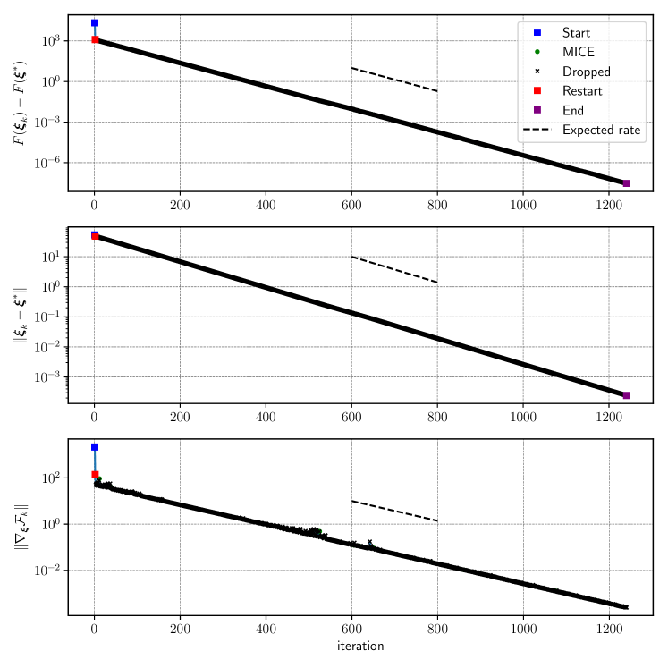
Figure 1. Single run, stochastic quadratic example, Equation (112) with $\kappa=100$ and $\epsilon=1$. Optimality gap (top), distance to the optimal point (center), and norm of gradient estimate (bottom) per iteration for SGD-MICE. The starting point, the restarts, and the end are marked respectively as blue, red, and purple squares, iterations dropped with black $\times$, and the remaining MICE points with green circles. SGD-MICE is able to achieve linear the $L^{2}$ convergence as predicted in Proposition 1.

In Figures 1 and 2, we present the optimality gap (109), the distance to the optimal point and the norm of the gradient estimate versus iteration and number of gradient evaluations, respectively. It Figure 2 we also plot the iteration per number of gradient evaluations. We mark the starting point, restarts, and ending point with blue, red, and purple squares, respectively; the dropped points with black $\times$, and the remaining iterations in the MICE hierarchy with green dots. In Figure 1, we depict that SGD-MICE attains the $L^{2}$ convergence with a constant step-size, as predicted in Proposition 1. In Figure 2, we present the convergence plots versus gradient evaluations, exhibiting numerical rates of $\mathcal{O}(M^{-\nicefrac{{1}}{{2}}})$ for the distance to the optimal point and for the norm of the gradient and of $\mathcal{O}(M^{-1})$ for the optimality gap. These rates are expected as the distance to the optimal point converges linearly (see Proposition 1) and the cost of sampling new gradients per iteration grows as $\mathcal{C}=\mathcal{O}(\|\nabla F(\boldsymbol{\xi}_{k})\|^{-2})$, as shown in (41). Consequently, since the objective function is quadratic, the convergence of the optimality gap is $\mathcal{O}(M^{-1})$. Note that the convergence is exponential as in the deterministic case until around $2\times 10^{4}$ gradient evaluations. After this point, there is a change of regime in which we achieve the asymptotic rates. We note that, after $2\times 10^{4}$, the cost of performing each iteration grows exponentially.

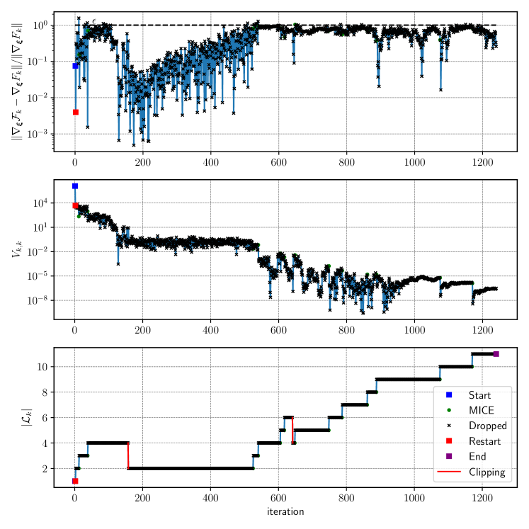
Figure 3. Single run, stochastic quadratic example, Equation (112) with $\kappa=100$ and $\epsilon=1$. Relative error in gradient estimates (top), estimated variances $V_{k,k}$ (center), and length of MICE hierarchy per iteration for SGD-MICE (bottom). The starting point, the restarts, and the end are marked respectively as blue, red, and purple squares, iterations dropped with black $\times$, and the remaining MICE points with green circles. The iterations where clipping is performed are marked with a red line. The tolerance on the statistical error is presented as a dashed line over the relative error in gradient estimates.

Figure 3 presents the relative error in gradient evaluations, the $V_{k,k}$, and the length of the hierarchy versus the number of iterations. Together with the relative error of the gradients, we plot the given tolerance on the statistical error, $\epsilon$. It can be observed that SGD-MICE is successful in keeping the relative error below $\epsilon$ and that most of the iterations are dropped with the hierarchy achieving a length of 11 after $1170$ iterations. Also, at around iterations $157$ and $641$, clipping can be observed, i.e., the hierarchy length is reduced without restarting it. Note that, when the first clipping is done, there is a significant reduction on the relative error. Once the relative statistical error becomes of size $\epsilon$, around iteration $k=500$ and $2\times 10^{4}$ gradient evaluations, the exponential convergence in Figure 2 is lost. The SGD-MICE algorithm drops all iterations from $180$ until $550$. When the relative error achieves $\epsilon$, it becomes advantageous to keep some iterations in the hierarchy, consequently progressively reducing the $V_{k,k}$. In the asymptotic regime, after iteration $1000$, two jumps can be seen in the $V_{k,k}$ exactly at the iterations where iterations are not dropped.

To verify if SGD-MICE indeed achieves the $L^{2}$ convergence predicted in §3.1, we perform a series of $1000$ independent runs for a few iterations arbitrarily close to the optimal point for SGD-MICE, idealized SGD-MICE (implemented as described in Appendix A), and the deterministic Gradient Descent (GD). In all cases we use the MICE step-size for strongly convex functions as presented in (66). Idealized SGD-MICE is devised to validate the theory presented in §3.1 when Assumptions 2, 3, and 4 are satisfied. Specifically, we want to test if the bias in MICE gradient estimates affects the $L^{2}$ convergence of SGD-MICE. In Figure 4, we present the mean-squared distance to the optimal point convergence for SGD-MICE, idealized SGD-MICE, and GD with confidence intervals of $99\%$ for each method using bootstrapping. For reference, we additionally plot the theoretical $L^{2}$ convergence for SGD-MICE. Two cases of $\kappa$ are presented, $\kappa=10$ and $100$; and two cases of $\epsilon$ are presented, $\epsilon=0.1$ and $1.0$. SGD-MICE performs as well as its idealized version, sometimes better. The better performance of SGD-MICE might be a consequence of the measures taken to make the algorithm robust, for instance, the resampling and $M_{min}$.

To validate the robustness and performance increase of SGD-MICE, we compare it with SGD using Monte Carlo sampling, at every iteration, to estimate the mean gradient, which we call SGD-A. Likewise SGD-MICE, SGD-A controls the relative statistical error in the mean gradient approximation and uses the resampling technique to estimate its norm.

In Figure 5, we present the optimality gap per iteration and number of gradient evaluations for SGD-A, SGD-MICE, and vanilla SGD (Robbins–Monro algorithm [30]). SGD-MICE appears to be more robust than SGD-A: the latter starts to oscillate once it gets close to the optimal point and thus is unable to maintain the linear convergence per iteration. Indeed, we performed $100$ independent runs of SGD-A and verified that, in all the runs, it oscillates in the same way as it gets close to the optimal point. Also, SGD-MICE requires less gradient evaluations to reduce the optimality gap than SGD-A. For vanilla SGD, we used a decreasing step-size of $\eta_{k}=(L(1+k/50))^{-1}$, tuned for the best performance of the method. When it comes to SGD, SGD-MICE performed better, achieving a lower optimality gap by several orders of magnitude for the same number of gradient evaluations.

Although this example is very simple, it illustrates the performance of SGD-MICE in an ideal situation where both $L$ and $\mu$ are known. Most importantly, we observed that the simplified theory presented in §2 and §3 still describes the behavior of SGD-MICE well; the linear $L^{2}$ convergence is achieved for the optimal step-size even with an $\epsilon=1.0$. Finally, SGD-MICE was able to automatically decide whether to drop iterations, restart, or clip the hierarchy to minimize the overall work required to attain the linear convergence per iteration.

Remark 13 (Alternative quadratic example).

Here, we aim instead at minimizing the expected value of

(115) $$f(\boldsymbol{\xi},\boldsymbol{\theta})\coloneqq(\boldsymbol{\xi}+\theta_{0}\mbox{\tenbfsl 1\/})\cdot\boldsymbol{H}\cdot(\boldsymbol{\xi}+\theta_{1}\mbox{\tenbfsl 1\/})\qquad\text{with}\qquad\boldsymbol{H}=\begin{bmatrix}100&3\\ 3&8\end{bmatrix}.$$

Here, 1 is a vector fully populated with ones, $\theta_{0}$ and $\theta_{1}$ are two independent, Gaussian $N(0,\sigma^{2})$ distributed, random variables. In this example, we performed numerical experiments, with $\sigma$ ranging from $10^{-4}$ to $10^{-1}$, to assess the efficiency of the couplings SGD-MICE and Adam-MICE. First, note that for two different values of $\boldsymbol{\xi}$, there is perfect correlation between the corresponding gradients, meaning that the variance of the gradient differences is zero. As a consequence, dropping occurs for all intermediate iterations and we only need one gradient difference sample at the current iteration point, $\boldsymbol{\xi}_{k}$. As we approach the optimal point $\boldsymbol{\xi}^{*},$ only the batch size at the initial point $\boldsymbol{\xi}_{0}$, that is, $M_{0,k}$, increases along the stochastic optimization process. In this example, MICE performs optimally and outperforms other alternatives.

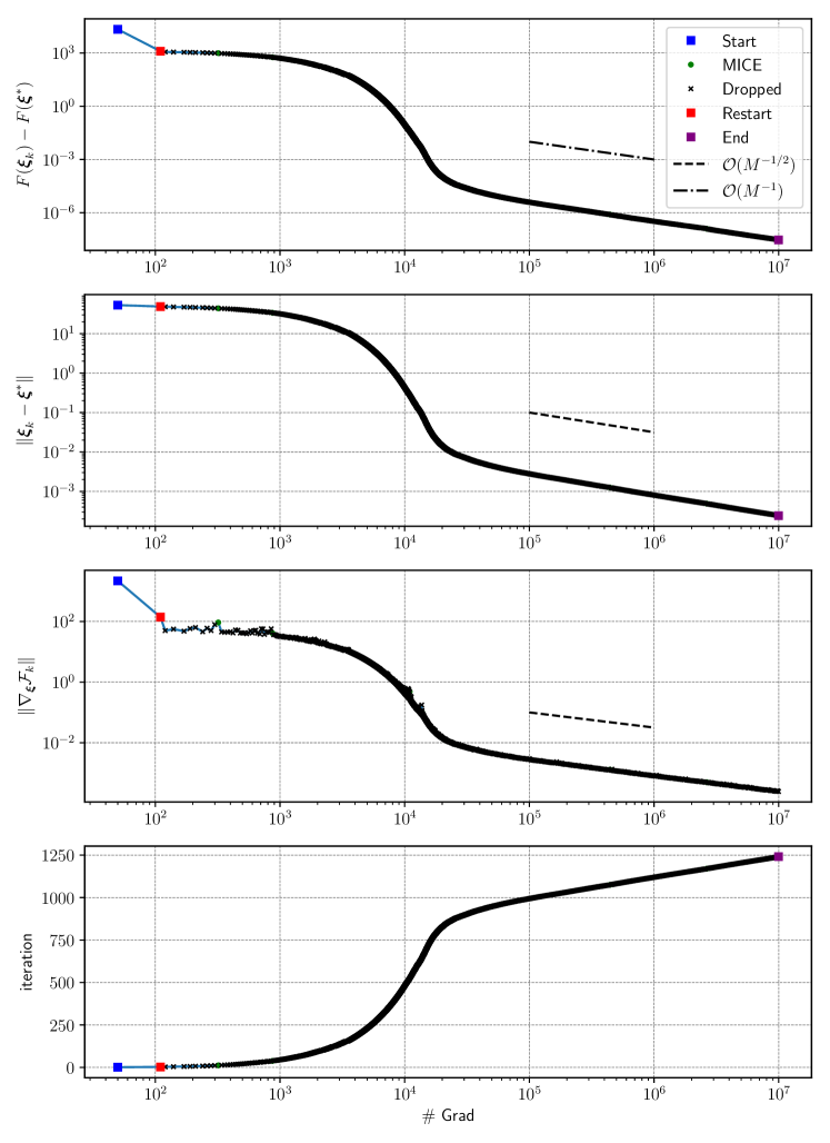
Figure 2. Single run, stochastic quadratic example, Equation (112) with $\kappa=100$ and $\epsilon=1$. Optimality gap (top), distance to the optimal point (center top), norm of gradient estimate (center bottom), and number of iterations (bottom) per number of gradient evaluations for SGD-MICE. The starting point, the restarts, and the end are marked respectively as blue, red, and purple squares, iterations dropped with black $\times$, and the remaining MICE points with green circles. The distance to the optimal point and the norm of the gradient achieve the Monte Carlo rate, $\mathcal{O}(M^{-\nicefrac{{1}}{{2}}})$ , whereas the optimality gap converges at the square of this rate, at $\mathcal{O}(M^{-1})$.

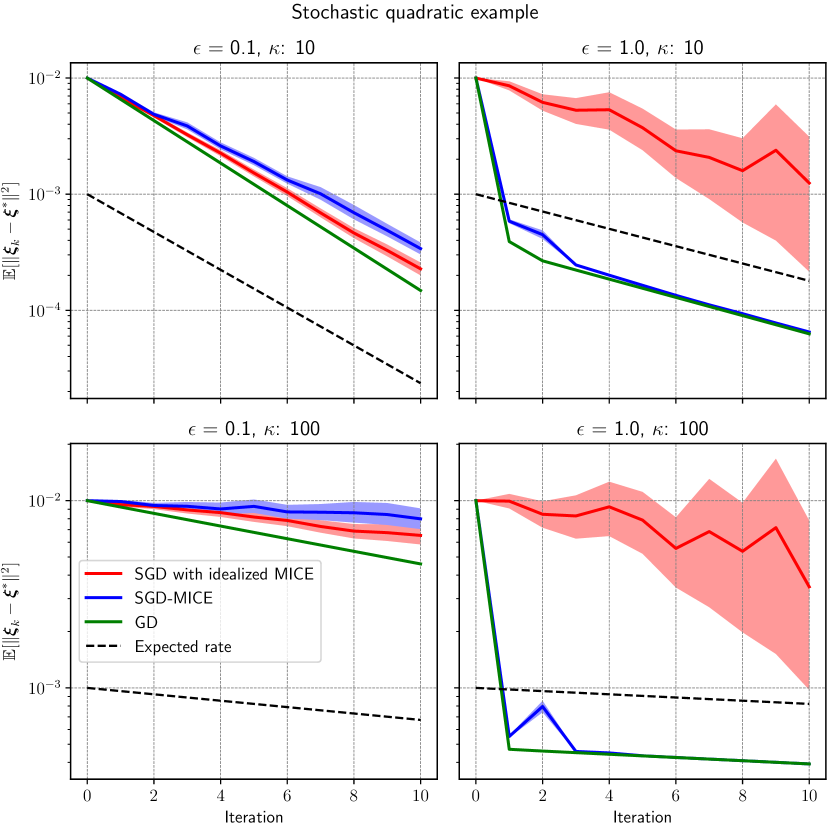
Figure 4. Estimates based on $1000$ independent runs. Stochastic quadratic example, Equation (112). Here, we plot estimates for the $L^{2}$ error studied in Proposition 1. We carry out this for SGD-MICE, SGD with the idealized MICE (see Appendix A), and gradient descent (GD) using the optimal SGD-MICE step-size for strongly convex functions, $\eta=\nicefrac{{2}}{{(L+\mu)(1+\epsilon^{2})}}$. The idealized MICE is implemented satisfying the conditions as presented in Proposition 1. In this case, we use the constants $\kappa$ as $10$ (top) and $100$ (bottom) and $\epsilon$ as $0.1$ (left) and $1.0$ (right). SGD-MICE achieves the theoretically predicted $L^{2}$ convergence rate, as can be observed by comparing it to the idealized SGD-MICE, showing numerically that, for this example, the bias in MICE estimates is negligible and does not affect the $L^{2}$ linear convergence rate. In fact, due to the minimum sample size and the resampling, for $\epsilon=1.0$, SGD-MICE performed better than theoretically predicted.

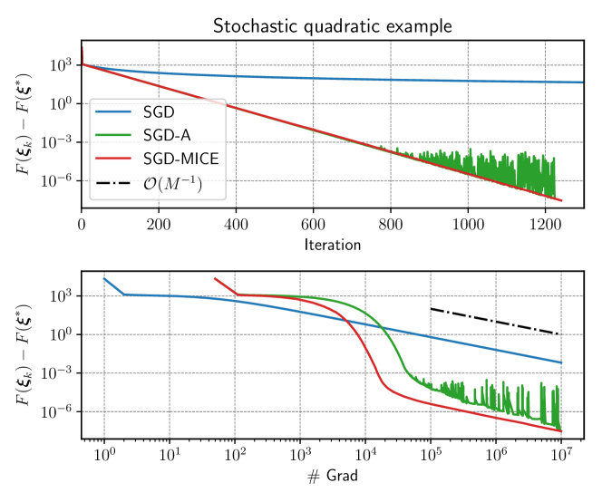
Figure 5. Single run, stochastic quadratic example, Equation (112) with $\kappa=100$ and $\epsilon=1$. For the sake of comparison, we solve this problem using SGD-MICE, vanilla SGD (Robbins–Monro algorithm [30]), and a version of SGD with fixed step-size and controlled variance, which we refer to as SGD-A. For SGD-A, we adaptively control the variance in gradient estimates by increasing the sample-size to keep the relative statistical error below a threshold, just as with SGD-MICE, also using the resampling technique to estimate the gradient norm. As for the tolerance on the statistical error and the resampling parameters, we used the same setup as for SGD-MICE. For SGD, we use a decreasing step-size of $\eta_{k}=1/(L+Lk/50)$, tuned to achieve the best performance possible. We present the optimality gap versus iterations (top) and the number of gradient evaluations (bottom) for the three versions of SGD. In the top figure, it can be observed that SGD-MICE is able to maintain stability in the asymptotic regime, whereas SGD-A oscillates. Moreover, SGD-MICE achieves better results for the same cost in terms of gradient evaluations than SGD-A during the optimization process. Thus, we can conclude that MICE not only improves the performance of stochastic gradient optimizers in terms of gradient evaluations as it also improves their stability in the asymptotic regime.

5.2. Stochastic Rosenbrock function

The goal of this example is to test the performance of Adam-MICE, that is, Adam coupled with our gradient estimator MICE, in minimizing the expected value of the stochastic Rosenbrock function in (117), showing that MICE can be coupled with different first-order optimization methods in a non-intrusive manner. Here we adapt the deterministic Rosenbrock function to the stochastic setting, specializing our optimization problem (1) with

(116) $$f(\boldsymbol{\xi},\boldsymbol{\theta})=\left(a-\xi_{0}+\theta_{0}\right)^{2}+b\left(-\xi_{0}^{2}+\xi_{1}+\theta_{0}^{2}-\theta_{1}^{2}\right)^{2},$$

where $a=1$, $b=100$, $\theta_{0},\theta_{1}\sim\mathcal{N}(0,\sigma_{\theta}^{2})$. The objective function to be minimized is thus

(117) $$F(\boldsymbol{\xi})=(a-\xi_{0})^{2}+\sigma_{\theta}^{2}+b\left(4\sigma_{\theta}^{4}+(\xi_{1}-\xi_{0}^{2})^{2}\right),$$

and its gradient is given by

(118) $$\nabla_{\boldsymbol{\xi}}F(\boldsymbol{\xi})=\begin{bmatrix}-2a+4b\xi_{0}^{3}-4b\xi_{0}\xi_{1}+2\xi_{0}\\ -2b\xi_{0}^{2}+2b\xi_{1}\end{bmatrix},$$

which coincides with the gradient of the deterministic Rosenbrock function. Therefore, the optimal point of the stochastic Rosenbrock is the same as the one of the deterministic: $\boldsymbol{\xi}^{*}=(a,a^{2})$. To perform the optimization, we sample the stochastic gradient

(119) $$\nabla_{\boldsymbol{\xi}}f(\boldsymbol{\xi},\boldsymbol{\theta})=\begin{bmatrix}-2a+4b\xi_{0}\left(\xi_{0}^{2}-\xi_{1}-\theta_{0}^{2}+\theta_{1}^{2}\right)+2\xi_{0}-2\theta_{0}\\ 2b\left(-\xi_{0}^{2}+\xi_{1}+\theta_{0}^{2}-\theta_{1}^{2}\right)\end{bmatrix}.$$

Although this is still a low dimensional example, minimizing the Rosenbrock function poses a difficult optimization problem for first-order methods; these tend to advance slowly in the region where the gradient has near-zero norm. Moreover, when noise is introduced in gradient estimates, their relative error can become large, affecting the optimization convergence.

We compare the convergence of the classical Adam algorithm against Adam-MICE. To illustrate the effect of the dispersion of the random variable $\boldsymbol{\theta}$, two distinct standard deviations are analyzed, namely $\sigma_{\theta}=10^{-4}$ and $\sigma_{\theta}=10^{-1}$. As for the optimization setup, we set Adam-MICE with fixed step-size $0.2$ and Adam with a decreasing step-size $\eta_{k}=\nicefrac{{0.02}}{{\sqrt{k}}}$, which we observed to be the best step-sizes for each method. The stopping criterion for both algorithms is set as $10^{7}$ gradient evaluations. For Adam-MICE, we use $\epsilon=0.7$, whereas for Adam we use a fixed batch size of $100$.

In Figures 6 and 7, we present, for $\sigma_{\theta}$ of $10^{-1}$ and $10^{-4}$, respectively, the optimality gap for both Adam and Adam-MICE versus the number of gradients, iterations, and runtime in seconds. It is clear that Adam-MICE is more stable than Adam, the latter oscillating as it approximates the optimal point in both cases. The efficient control of the error in gradient estimates allows Adam-MICE to converge monotonically in the asymptotic phase. Moreover, the number of iterations and the runtime are much smaller for Adam-MICE than for Adam.

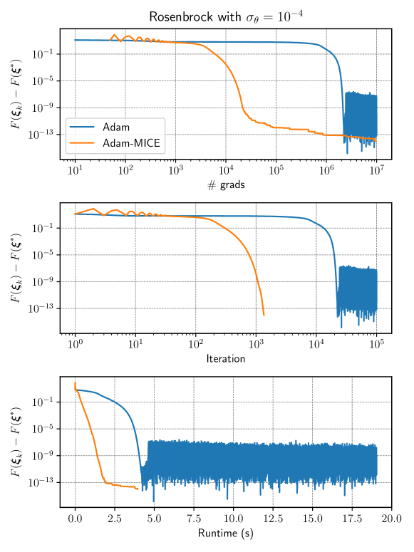
Figure 6. Single run, stochastic Rosenbrock function example, Equation (117) with $\sigma_{\theta}=10^{-4}$. Optimality gap for Adam and Adam-MICE versus number of gradient evaluations (top), iterations (center), and runtime in seconds (bottom).

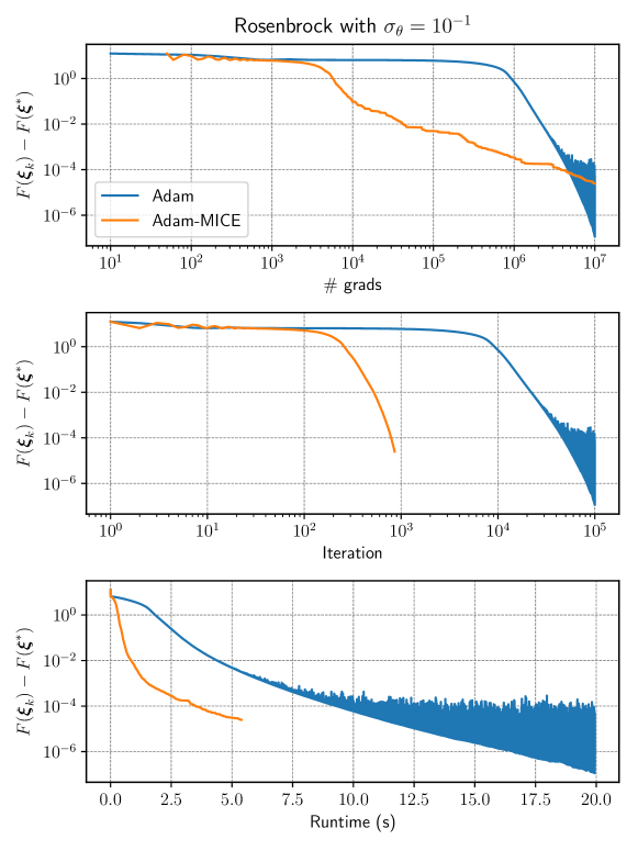
Figure 7. Single run, stochastic Rosenbrock function example, Equation (117) with $\sigma_{\theta}=10^{-1}$. Optimality gap for Adam and Adam-MICE versus number of gradient evaluations (top), iterations (center), and runtime in seconds (bottom).

5.3. Logistic regression

In this example, we train logistic regression models using SGD-MICE, SAG [45], SAGA [26], SARAH [23], and SVRG [22] to compare their performances. Here, we present a more practical application of MICE, where we can test its performance on high-dimensional settings with finite populations. Therefore, we calculate the statistical error as in Remark 7 and use (43) to obtain the optimal sample sizes. To train the logistic regression model for binary classification, we use the $\ell_{2}$-regularized log-loss function

(120) $$F(\boldsymbol{\xi})=\frac{1}{N}\sum_{i=1}^{N}f\left(\boldsymbol{\xi},\boldsymbol{\theta}_{i}=(\boldsymbol{x}_{i},y_{i})\right)=\frac{1}{N}\sum_{i=1}^{N}\log(1+\exp(-y_{i}\boldsymbol{\xi}\cdot\boldsymbol{x}_{i}))+\frac{\lambda}{2}\|\boldsymbol{\xi}\|^{2},$$

where each data point $(\boldsymbol{x}_{i},y_{i})$ is such that $\boldsymbol{x}_{i}\in\mathbb{R}^{d_{\boldsymbol{\xi}}}$ and $y_{i}\in\{-1,1\}$. We use the datasets mushrooms, gisette, and Higgs, obtained from LibSVM. The size of the datasets $N$, number of features $d_{\boldsymbol{\xi}}$, and regularization parameters $\lambda$ are presented in Table 1.

Table 1. Size, number of features, and regularization parameters for the datasets used in the logistic regression example.

Dataset	Size	Number of features	$\lambda$
mushrooms	8124	112	$10^{-5}$
gisette	6000	5000	$10^{-4}$
HIGGS	11000000	28	$10^{-4}$

When using SGD-MICE for training the logistic regression model, we use $\epsilon=0.5$. For the other methods, we use batchsizes of size $10$. Since we have finite populations, we use (43) to calculate the sample-sizes. SGD-MICE step is based on the Lipschitz smoothness and strong-convexity constant of the true objective function as presented in Proposition 1. Conversely, the other methods rely on a Lipschitz constant that must hold a.s., which we refer to as $L_{\text{a.s.}}$. The step-sizes for SAG, SAGA, SARAH, and SVRG are presented in Table 2. These steps were chosen as the best performing for each case based on the recommendations of their original papers.

Table 2. Step-sizes chosen for each method for the logistic regression example.

Method	SAG	SAGA	SARAH	SVRG
Step-size	$\frac{1}{16(L_{\text{a.s.}}+\mu N)}$	$\frac{1}{2(L_{\text{a.s.}}+\mu N)}$	$\frac{1}{2L_{\text{a.s.}}}$	$\frac{1}{2L_{\text{a.s.}}}$

Figures 8, 9, and 10 present the relative optimality gap (the optimality gap normalized by its starting value) for, respectively, the mushrooms, gisette, and HIGGS datasets versus the number of gradient evaluations, iterations and runtime in seconds. In the mushrooms dataset, SGD-MICE decreases the optimality gap more than the other methods for the same number of gradient samples during the whole optimization process. Moreover, the total number of iterations is much smaller than for the other methods. However, the overhead of our SGD-MICE implementation becomes plain to see when we compare the runtimes; the current implementation of SGD-MICE is more costly than the other methods. In the gisette dataset, the overall behavior of the methods is the same as in the first data set. Finally, for the HIGGS dataset, which is a much larger dataset, SGD-MICE performs better than the other methods both in the number of gradient evaluations and in runtime. Moreover, SGD-MICE performed around $2\times 10^{3}$ iterations while the other methods required more than $10^{6}$ iterations.

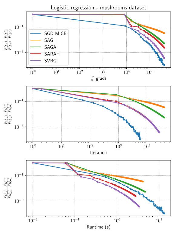
Figure 8. Single run, logistic regression example, Equation (120) for the mushrooms dataset. Relative optimality gap versus number of gradient evaluations (top), iterations (center), and runtime in seconds (bottom) for SGD-MICE, SAG, SAGA, SARAH, and SVRG.

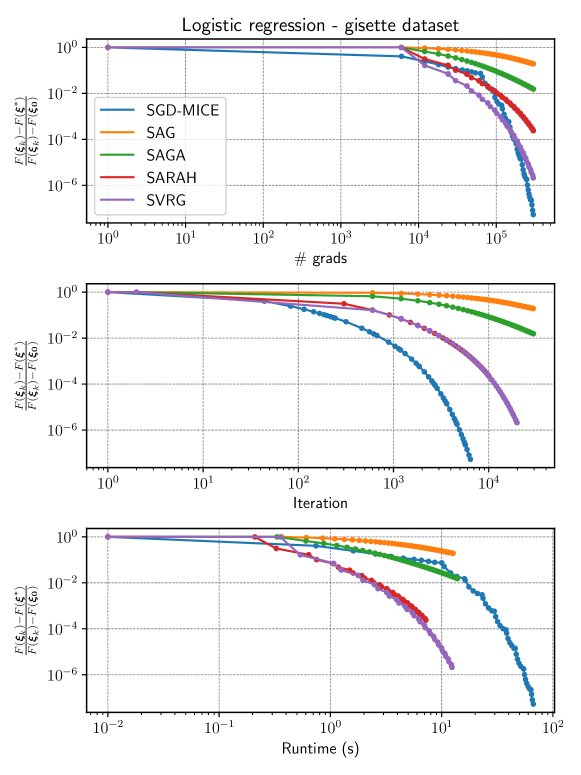
Figure 9. Single run, logistic regression example, Equation (120) for the gisette dataset. Relative optimality gap versus number of gradient evaluations (top), iterations (center), and runtime in seconds (bottom) for SGD-MICE, SAG, SAGA, SARAH, and SVRG.

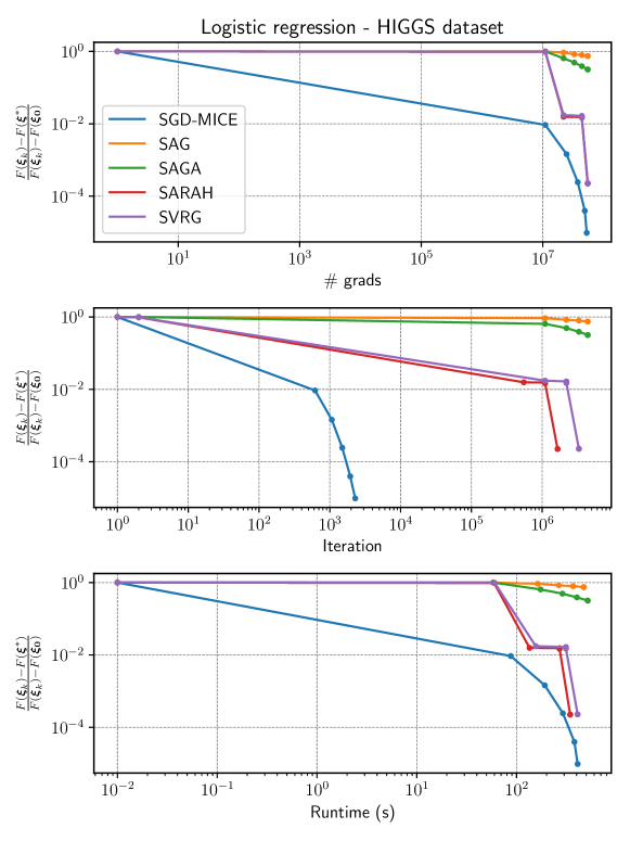
Figure 10. Single run, logistic regression example, Equation (120) for the HIGGS dataset. Relative optimality gap versus number of gradient evaluations (top), iterations (center), and runtime in seconds (bottom) for SGD-MICE, SAG, SAGA, SARAH, and SVRG.

From the results of this example, we observe that MICE performs well in problems with a reasonably large number of parameters, for instance, $5000$ in the gisette, and finite dataset populations ranging from the thousands to the millions. Moreover, it seems that SGD-MICE’s performance compared to the other methods increases as the population size grows. Note that both SAG and SAGA need to decrease their step-sizes as the sample-size increases, and that SARAH and SVRG need to reevaluate the full-gradient after a few epochs to keep their convergence.

6. Acknowledgments

This work was partially supported by the KAUST Office of Sponsored Research (OSR) under Award numbers URF$/1/2281-01-01$, URF$/1/2584-01-01$ in the KAUST Competitive Research Grants Program Round 8, the Alexander von Humboldt Foundation, and Coordination for the Improvement of Higher Education Personnel (CAPES).

Last but not least, we want to thank Dr. Sören Wolfers and Prof. Jesper Oppelstrup. They both provided us with valuable ideas and constructive comments.

7. Conclusion

We propose the Multi-Iteration Stochastic Optimizers, a novel class of first-order stochastic optimizers. To build this class, we presented an estimator of the mean gradient Multi-Iteration stochastiC Estimator—MICE—based on successive control variates along the path of iterations. MICE uses a hierarchy based on previously computed sample gradients from iterations in the optimization path. At each iteration, MICE samples new gradients to achieve a desired relative tolerance on the gradient’s statistical error with minimal computational cost. We coupled MICE with techniques to automatically update its hierarchy. These updates selectively perform restarting, dropping iterations, or clipping the hierarchy to minimize the computational work. Furthermore, to robustify the use of MICE, we use a jackknife resampling technique to estimate the norm of the mean gradient. This norm estimate is useful for picking the optimizer’s step length, thus controlling MICE’s relative statistical error. Due to its nonintrusive nature, it is relatively simple to couple MICE with many existing first-order optimization methods, resulting in a new family of optimizers.

An idealized theoretical analysis for Stochastic Gradient Descent coupled with the MICE estimator (SGD-MICE) is provided for $L$-smooth and strongly-convex functions. In this context, we motivate the relative error control’s usefulness in the mean gradient estimates, proving exponential convergence in $L^{2}$ sense with respect to the number of iterations using a constant step-size. We also estimate the resulting mean computational cost in terms of the number of sampled gradients.

To test the performance of this new family of optimizers, we present three numerical examples. In all three examples, with either finite and infinite populations, we use the same parameters for MICE, changing only the tolerance on the statistical error. The first example is a quadratic function with a stochastic Hessian, used to verify our analysis. We compare SGD-MICE with the expected convergence rates in terms of iterations and gradient evaluations. The second example is an adaptation of the Rosenbrock function to the stochastic setting, where we use Adam-MICE and Adam to perform optimization. The third example consists of training a logistic regression model over three different datasets, one of which is $11\times 10^{6}$, showing that SGD-MICE can outperform common optimization methods, such as SGD, SAG, SAGA, SRVG, and SARAH, in these supervised machine learning problems with large datasets.

Finally, although in this work we only address unconstrained optimization, one can use similar MICE estimators in constrained optimization, reusing all the standard techniques, for instance, projected gradients, active sets, among others.

Appendix A Stochastic gradient descent with idealized MICE

This section describes the stochastic gradient descent with Gaussian noise in gradients satisfying Assumption 4, which we call stochastic gradient descent with idealized MICE. We focus on the case where Assumptions 2 and 3 are also satisfied. This method is not a practical stochastic optimization method since we use the exact mean gradient to generate a noisy gradient estimate. The goal of this artificial method is to validate Proposition 1 and Corollary 1 on, respectively, the $L^{2}$ and a.s. convergence rates of SGD-MICE. If the bias of MICE and the errors in gradient norm and variances are negligible, SGD-MICE should behave like idealized SGD-MICE. Thus, by comparing SGD-MICE with idealized SGD-MICE, we can verify how close SGD-MICE is to achieving the $L^{2}$ and a.s. convergences in Proposition 1 and Corollary 1.

To implement idealized SGD-MICE, we add Gaussian noise to the true gradient and use it as an estimate of the gradient in SGD in such a way that Assumption 4 is satisfied. For a true gradient $\nabla_{\boldsymbol{\xi}}F(\boldsymbol{\xi}_{k})$ and a covariance matrix $\boldsymbol{\Sigma}$ of $\nabla_{\boldsymbol{\xi}}f(\boldsymbol{\xi},\boldsymbol{\theta})$, we define the mean gradient estimate $\tilde{\boldsymbol{\upsilon}}$ as

(121) $$\tilde{\boldsymbol{\upsilon}}=\nabla_{\boldsymbol{\xi}}F(\boldsymbol{\xi})+\frac{\epsilon\|\nabla_{\boldsymbol{\xi}}F(\boldsymbol{\xi})\|}{\sqrt{\hbox{{tr}}\mskip 2.0mu(\boldsymbol{\Sigma})}}\boldsymbol{\chi},$$

where $\boldsymbol{\chi}\sim\mathcal{N}(\boldsymbol{0},\boldsymbol{\Sigma})$. Taking the expectation of $\tilde{\boldsymbol{\upsilon}}$ conditioned on $\{\boldsymbol{\xi}_{\ell}\}_{\ell\in\mathcal{L}_{k}}$,

(122) $$\mathbb{E}[\tilde{\boldsymbol{\upsilon}}_{k}|\{\boldsymbol{\xi}_{\ell}\}_{\ell\in\mathcal{L}_{k}}]=\nabla_{\boldsymbol{\xi}}F(\boldsymbol{\xi}_{k}),$$

and taking the expectation of mean squared error conditioned on $\{\boldsymbol{\xi}_{\ell}\}_{\ell\in\mathcal{L}_{k}}$ we see that

(123) $$\mathbb{E}[\left\lVert{\nabla_{\boldsymbol{\xi}}F(\boldsymbol{\xi}_{k})-\tilde{\boldsymbol{\upsilon}}_{k}}\right\rVert^{2}|\{\boldsymbol{\xi}_{\ell}\}_{\ell\in\mathcal{L}_{k}}]=\epsilon^{2}\left\lVert{\nabla_{\boldsymbol{\xi}}F(\boldsymbol{\xi}_{k})}\right\rVert^{2},$$

hence, Assumption 4 holds. Consequently, idealized SGD-MICE $L^{2}$ and a.s. convergences follow Proposition 1 and Corollary 1, respectively.

Appendix B Multi-iteration stochastic optimizers

In this section, we present the detailed algorithms for the multi-iteration stochastic optimizers using the MICE estimator for the mean gradient. In Algorithms 2, 3, we respectively describe the pseudocodes for SGD-MICE and Adam-MICE.

Algorithm 2 Pseudocode for the SGD-MICE with fixed step-size. SGD-MICE requires an unbiased estimator of the true gradient, $\nabla f$; a starting point, $\boldsymbol{\xi}_{0}$; a step-size, $\eta$; and a distribution from which $\boldsymbol{\theta}$ can be sampled, $\pi$.

1:procedure SGD-MICE($\nabla_{\boldsymbol{\xi}}f$, $\boldsymbol{\xi}_{0},\eta,\pi$)

2:     for $k=0,1,2...K$ do

3:         Evaluate $\nabla_{\boldsymbol{\xi}}\mathcal{F}_{k}$ using Algorithm 1

4:         $\boldsymbol{\xi}_{k+1}\leftarrow\boldsymbol{\xi}_{k}-\eta\nabla_{\boldsymbol{\xi}}\mathcal{F}_{k}$

5:     end for

6:     return optimal point approximation $\boldsymbol{\xi}_{K+1}$

7:end procedure

Algorithm 3 Pseudocode for the Adam-MICE with fixed step-size. Adam-MICE requires an unbiased estimator of the true gradient, $\nabla_{\boldsymbol{\xi}}f$; a starting point, $\boldsymbol{\xi}_{0}$; a step-size, $\eta$; and a distribution from which $\boldsymbol{\theta}$ can be sampled, $\pi$. Moreover, Adam-MICE requires the constants $\beta_{1}$, $\beta_{2}$, and $\epsilon_{\text{Adam}}$. We use the values recommended by [31], $\beta_{1}=0.9$, $\beta_{2}=0.999$, and $\epsilon_{\text{Adam}}=10^{-8}$.

1:procedure Adam-MICE($\nabla_{\boldsymbol{\xi}}f$, $\boldsymbol{\xi}_{0},\eta,\pi$)

2:     Initialize $\boldsymbol{m}_{0}$ and $\boldsymbol{v}_{0}$ as zero-vectors

3:     for $k=1,2...K$ do

4:         Evaluate $\nabla_{\boldsymbol{\xi}}\mathcal{F}_{k}$ using Algorithm 1

5:         $\boldsymbol{m}_{k}\leftarrow\beta_{1}\boldsymbol{m}_{k-1}+(1-\beta_{1})\nabla_{\boldsymbol{\xi}}\mathcal{F}_{k}$

6:         $\boldsymbol{v}_{k}\leftarrow\beta_{2}\boldsymbol{v}_{k-1}+(1-\beta_{2})\nabla_{\boldsymbol{\xi}}\mathcal{F}_{k}^{2}$ $\triangleright$ The gradient estimates are squared element-wise

7:         $\boldsymbol{\hat{m}}_{k}\leftarrow\boldsymbol{m}_{k-1}/(1-\beta_{1}^{k})$

8:         $\boldsymbol{\hat{v}}_{k}\leftarrow\boldsymbol{v}_{k-1}/(1-\beta_{2}^{k})$

9:         $\boldsymbol{\xi}_{k+1}\leftarrow\boldsymbol{\xi}_{k}-\eta\boldsymbol{\hat{m}}_{k}/(\sqrt{\boldsymbol{\hat{v}}_{k}}+\epsilon_{\text{Adam}})$

10:     end for

11:     return optimal point approximation $\boldsymbol{\xi}_{K+1}$

12:end procedure

References

• [1] K. Marti. Stochastic optimization methods, volume 2. Springer, 2005.
• [2] S. Uryasev and P.M. Pardalos. Stochastic optimization: algorithms and applications, volume 54. Springer Science & Business Media, 2013.
• [3] J.R. Birge and F. Louveaux. Introduction to Stochastic Programming. Springer Publishing Company, Incorporated, 2nd edition, 2011.
• [4] G. Lan. First-order and Stochastic Optimization Methods for Machine Learning. Springer, 2020.
• [5] S.W. Wallace and W.T. Ziemba. Applications of stochastic programming. SIAM, 2005.
• [6] W.H. Fleming and R.W. R. Deterministic and stochastic optimal control, volume 1. Springer Science & Business Media, 2012.
• [7] W.T. Ziemba and R.G. Vickson. Stochastic optimization models in finance. Academic Press, 2014.
• [8] A.J. Conejo, M. Carrión, J.M. Morales, et al. Decision making under uncertainty in electricity markets, volume 1. Springer, 2010.
• [9] C. Bayer, R. Tempone, and S. Wolfers. Pricing American options by exercise rate optimization. Quant. Finance, 20(11):1749–1760, 2020.
• [10] F.-R. Chang. Stochastic optimization in continuous time. Cambridge University Press, 2004.
• [11] P. Azcue and N. Muler. Stochastic optimization in insurance. SpringerBriefs in Quantitative Finance. Springer, New York, 2014. A dynamic programming approach.
• [12] Z. Ding. Stochastic Optimization and Its Application to Communication Networks and the Smart Grid. University of Florida Digital Collections. University of Florida, 2012.
• [13] D.D. Yao, H. Zhang, and X.Y. Zhou, editors. Stochastic modeling and optimization. Springer-Verlag, New York, 2003. With applications in queues, finance, and supply chains.
• [14] E.G. Ryan, C.C. Drovandi, J.M. McGree, and A.N. Pettitt. A review of modern computational algorithms for bayesian optimal design. International Statistical Review, 84(1):128–154, 2016.
• [15] A.G. Carlon, B.M. Dia, L. Espath, R.H. Lopez, and R. Tempone. Nesterov-aided stochastic gradient methods using laplace approximation for bayesian design optimization. Computer Methods in Applied Mechanics and Engineering, 363, 2020.
• [16] S. Heinrich. The multilevel method of dependent tests. In Advances in stochastic simulation methods, pages 47–61. Springer, 2000.
• [17] M.B. Giles. Multilevel Monte Carlo path simulation. Operations research, 56(3):607–617, 2008.
• [18] D. Ruppert. Efficient estimations from a slowly convergent robbins-monro process. Technical report, Cornell University Operations Research and Industrial Engineering, 1988.
• [19] R.H. Byrd, G.M. Chin, J. Nocedal, and Y. Wu. Sample size selection in optimization methods for machine learning. Mathematical programming, 134(1):127–155, 2012.
• [20] L. Balles, J. Romero, and P. Hennig. Coupling adaptive batch sizes with learning rates. arXiv preprint arXiv:1612.05086, 2016.
• [21] R. Bollapragada, R. Byrd, and J. Nocedal. Adaptive sampling strategies for stochastic optimization. SIAM Journal on Optimization, 28(4):3312–3343, 2018.
• [22] R. Johnson and T. Zhang. Accelerating stochastic gradient descent using predictive variance reduction. In Advances in neural information processing systems, pages 315–323, 2013.
• [23] L.M. Nguyen, J. Liu, K. Scheinberg, and M. Takáč. Sarah: A novel method for machine learning problems using stochastic recursive gradient. In Proceedings of the 34th International Conference on Machine Learning-Volume 70, pages 2613–2621. JMLR. org, 2017.
• [24] L. Nguyen, K. Scheinberg, and M. Takáč. Inexact sarah algorithm for stochastic optimization. Optimization methods & software, 08 2020.
• [25] C. Fang, C.J. Li, Z. Lin, and T. Zhang. Spider: Near-optimal non-convex optimization via stochastic path-integrated differential estimator. In Advances in Neural Information Processing Systems, pages 689–699, 2018.
• [26] A. Defazio, F. Bach, and S. Lacoste-Julien. Saga: A fast incremental gradient method with support for non-strongly convex composite objectives. In Advances in neural information processing systems, pages 1646–1654, 2014.
• [27] M.P. Friedlander and M. Schmidt. Hybrid deterministic-stochastic methods for data fitting. SIAM Journal on Scientific Computing, 34(3):A1380–A1405, 2012.
• [28] S. De, A. Yadav, D. Jacobs, and T. Goldstein. Big batch sgd: Automated inference using adaptive batch sizes. arXiv preprint arXiv:1610.05792, 2016.
• [29] K. Ji, Z. Wang, Y. Zhou, and Y. Liang. Faster stochastic algorithms via history-gradient aided batch size adaptation. arXiv preprint arXiv:1910.09670, 2019.
• [30] H. Robbins and S. Monro. A stochastic approximation method. The annals of mathematical statistics, pages 400–407, 1951.
• [31] D. P Kingma and J. Ba. Adam: A method for stochastic optimization. arXiv preprint arXiv:1412.6980, 2014.
• [32] J.C. Spall. Introduction to stochastic search and optimization: estimation, simulation, and control, volume 65. John Wiley & Sons, 2005.
• [33] A. Shapiro, D. Dentcheva, and A. Ruszczyński. Lectures on stochastic programming: modeling and theory. SIAM, 2014.
• [34] A. Nitanda. Stochastic proximal gradient descent with acceleration techniques. In Advances in Neural Information Processing Systems, pages 1574–1582, 2014.
• [35] J. Konečnỳ, J. Liu, P. Richtárik, and M. Takáč. Mini-batch semi-stochastic gradient descent in the proximal setting. IEEE Journal of Selected Topics in Signal Processing, 10(2):242–255, 2016.
• [36] S. Heinrich. Multilevel Monte Carlo methods. In Large-Scale Scientific Computing, volume 2179 of Lecture Notes in Computer Science, pages 58–67. Springer Berlin Heidelberg, 2001.
• [37] M.B. Giles. Multilevel monte carlo methods. Acta Numerica, 24:259–328, 2015.
• [38] S. Dereich and T. Müller-Gronbach. General multilevel adaptations for stochastic approximation algorithms of Robbins-Monro and Polyak-Ruppert type. Numer. Math., 142(2):279–328, 2019.
• [39] S. Yang, M. Wang, and E.X. Fang. Multilevel stochastic gradient methods for nested composition optimization. SIAM Journal on Optimization, 29(1):616–659, 2019.
• [40] L. Isserlis. On the value of a mean as calculated from a sample. Journal of the Royal Statistical Society, 81(1):75–81, 1918.
• [41] B. Efron. The jackknife, the bootstrap, and other resampling plans, volume 38. Siam, 1982.
• [42] Y. Nesterov. Lectures on convex optimization, volume 137. Springer, 2018.
• [43] A. Nemirovski. Efficient methods in convex programming. Lecture notes, 1994.
• [44] B.P. Welford. Note on a method for calculating corrected sums of squares and products. Technometrics, 4(3):419–420, 1962.
• [45] M. Schmidt, N. Le Roux, and F. Bach. Minimizing finite sums with the stochastic average gradient. Mathematical Programming, 162(1-2):83–112, 2017.