Wrinkling transition in quenched disordered membranes at two loops

Abstract

We investigate the flat phase of quenched disordered polymerized membranes by means of a two-loop, weak-coupling computation performed near their upper critical dimension $D_{uc}=4$, generalizing the one-loop computation of Morse et al. [Phys. Rev. A 45, R2151 (1992), Phys. Rev. A 46, 1751 (1992)]. Our work confirms the existence of the finite-temperature, finite-disorder, wrinkling transition, which has been recently identified by Coquand et al.[Phys. Rev E 97, 030102 (2018)] using a nonperturbative renormalization group approach. We also point out ambiguities in the two-loop computation that prevent the exact identification of the properties of the novel fixed point associated with the wrinkling transition, which very likely requires a three-loop order approach.

Introduction

The critical and, more generally, the long-distance equilibrium statistical physics of pure, homogeneous, systems is now widely understood. By contrast, quenched, random heterogeneities, such as defects or impurities, inevitably present in most real physical systems, are known to give rise to a wide spectrum of new phenomena. Quenched disordered membranes occupy a special place; see e.g. Radzihovsky (2004), as their most famous physical realizations seem to bring out the physical effects of both random bonds and random fields; see Dotsenko (2001); Young (1998); T. Nattermann (1999); De Dominicis et al. (1998); De Dominicis and Giardina (2006); K. J. Wiese and P. Le Doussal (2007); Tarjus and Tissier (2020) for reviews. For instance, in a series of experiments beginning in the early 90’s, Mutz et al. M. Mutz, D. Bensimon, and M. J. Brienne (1991) then Chaieb et al. S. Chaieb, V.K. Natrajan, and A. A. El-rahman (2006); Chaieb et al. (2008) have shown that, upon cooling below the chain melting temperature, photo-induced partially polymerized vesicles made of diacetylenic phospholipid undergo a transition from a smooth structure, at high polymerization, to a wrinkled structure, at low polymerization, with randomly frozen normals that could characterize a glassy phase. This transition and the resulting wrinkled phase have been conjectured to result from the joint effects of random heterogeneities on both the internal metric and the curvature of the membrane Radzihovsky and D. R. Nelson (1991) that bear formal similarities with, respectively, random bonds and random fields in magnetic systems; see below. More recently, in the context of the rapidly growing defect engineering Banhart et al. (2011); Liu et al. (2015); G. Yang, L. Li, W. B. Lee and M.C. Ng (2018); B. Ni, T. Zhang, J. Li, X. Li and H. Gao (2019) of graphene Novoselov et al. (2004, 2005), it has been shown that by thoroughly damaging a clean sheet of this material with a laser beam, it was possible to induce a crystal-to-glass transition giving rise to a vacancy-amorphized graphene structure J. Kotakoski, A.V. Krasheninnikov, U. Kaiser and J.C. Meyer (2011); F.R. Eder, J. Kotakoski, U. Kaiser and J.C. Meyer (2014); W.-J. Joo et al (2017). Here also, the inclusion of lattice defects – foreign adatoms or substitutional impurities – is expected to lead, in addition to metric alterations, to a rearrangement of sp²-hybridized carbon atoms into nonhexagonal structures and, thus, to the generation of nonvanishing curvature structures showing again that the underlying physics could rely on the coexistence of the two kinds of disorder.

Disordered membranes also stand out from the crowd by the theoretical investigations to which they have been subjected. Stimulated by the work of Mutz et al. M. Mutz, D. Bensimon, and M. J. Brienne (1991) on partially polymerized vesicles, the first attempt to probe the effects of disorder in membranes has been realized by Nelson and Radzihovsky Nelson and Radzihovsky (1991); Radzihovsky and D. R. Nelson (1991), who have focused their study on the role of disorder in the preferred metric. Performing a weak-coupling expansion near the upper critical dimension $D_{\hbox{\scriptsize uc}}=4$ they have shown that, for $D<4$, while the disorder is irrelevant and the renormalization group (RG) flow is driven toward the disorder-free fixed point – $P_{4}$ – at any finite temperature, an instability close to $T=0$ could be accompanied by a diverging Edwards-Anderson correlation length, leading to a glassy phase. Then Radzihovsky and Le Doussal Radzihovsky and P. Le Doussal (1992), by employing a large embedding dimension $d$-expansion, have confirmed such a possibility, finding an instability of the flat phase toward a spin-glass-like phase. However no quantitative or qualitative empirical confirmation of this scenario has been provided. Morse et al. D. C. Morse, T. C. Lubensky and G. S. Grest (1992); D. C. Morse and T. C. Lubensky (1992) have then reconsidered the weak-coupling analysis of Ref.Nelson and Radzihovsky (1991); Radzihovsky and D. R. Nelson (1991) within an approach including both metric and curvature disorders. They have confirmed the irrelevance of the disorder in $D<4$ but shown that the presence of curvature disorder gives rise to a new and vanishing temperature fixed point – $P_{5}$ – stable with respect to randomness but unstable with respect to the temperature. Somewhat disappointing from the point of view of the search for a new exotic phase, these works have been followed mainly by mean-field approximations involving either short-range Radzihovsky and P. Le Doussal (1992); Bensimon et al. (1992, 1993); R. Attal, S. Chaieb, and D. Bensimon (1993); Park and Kwon (1996); Mori (1996); Benyoussef et al. (1998) or long-range Le Doussal and Radzihovsky (1993); Mori and Wadati (1994) disorder leading to speculate about the existence of a glassy phase at any temperature and for large enough disorder; see P. Le Doussal and L. Radzihovsky (2018) for a review. Again no confirmation of this conjecture has been provided. However very recently, an approach based on the nonperturbative renormalization group (NPRG), following those performed on disorder-free membranes J.-P. Kownacki and Mouhanna (2009); F. L. Braghin and N. Hasselmann (2010); Essafi et al. (2011); N. Hasselmann and F. L. Braghin (2011); Essafi et al. (2014); Coquand and Mouhanna (2016) has been realized by Coquand et al. Coquand et al. (2018) on the model considered by Morse and Lubensky displaying both metric and curvature disorders. Their main result has been to identify a novel finite temperature, finite disorder fixed-point – $P_{c}$ – once unstable, and thus associated with a second-order phase transition and making the $T=0$ fixed point fully attractive provided $T<T_{c}$. This study has allowed the identification of three distinct universal scaling behaviors Coquand et al. (2020a) corresponding both qualitatively and quantitatively to those observed in the experiments of Chaieb et al S. Chaieb, V.K. Natrajan, and A. A. El-rahman (2006); Chaieb et al. (2008).

Whereas the NPRG results have been challenged within a recent self-consistent screening approximation approach P. Le Doussal and L. Radzihovsky (2018) they have been confirmed within a large $d$ approach performed at next-to-leading order in $1/d$ D. R. Saykin, V. Yu. Kachorovskii and I. S. Burmistrov (2020) although in a model involving only curvature disorder. In this controversial context, it was compelling to further investigate the model of Morse et al. D. C. Morse, T. C. Lubensky and G. S. Grest (1992); D. C. Morse and T. C. Lubensky (1992). In that respect, an essential feature of the novel fixed point $P_{c}$ found in Coquand et al. (2018) is that its coordinates near $D_{\hbox{\scriptsize uc}}=4$ differ only from those of the vanishing temperature fixed point $P_{5}$ by terms of order $\epsilon^{2}$, with $\epsilon=4-D$, strongly suggesting that $P_{c}$ could be also identified within a perturbative $\epsilon$-expansion up to this order. This is the reason why we investigate, in this letter, quenched disordered membranes at two-loops in the vicinity of the upper critical dimension, extending both the one-loop computation of Morse et al. performed 30 years ago D. C. Morse, T. C. Lubensky and G. S. Grest (1992); D. C. Morse and T. C. Lubensky (1992), at the next order and the recent two-loop computation of Coquand et al. Coquand et al. (2020b) – see also A. Mauri and M.I. Katsnelson (2020) – on disorder-free membranes, to the disordered case. We derive the RG equations, analyze them and provide the critical quantities, notably the anomalous dimension $\eta$, at order $\epsilon^{2}$. Our approach confirms unambiguously the existence of the once-unstable fixed point $P_{c}$ characterizing a phase transition between a high-temperature phase controlled by the disorder-free fixed point $P_{4}$ and a low-temperature phase controlled by the vanishing-temperature, finite-disorder, fixed point $P_{5}$ . It nevertheless reveals also a drawback of the perturbative approach at two-loop order which manifests through the impossibility to identify exactly the location and properties of the fixed points $P_{5}$ and $P_{c}$ at this order; we argue that this should very likely be raised by a three-loop order computation.

The action

A membrane is modelized by a $D$-dimensional surface embedded in a $d$-dimensional Euclidean space. A point on the membrane is thus identified by $D$-dimensional vector ${\bf x}$ and a configuration of the membrane in the Euclidean space is described through the embedding ${\bf x}\to{\bf R}({\bf x})$ with ${\bf R}\in\mathbb{R}^{d}$. In the flat phase we define the average position of a point ${\bf x}$:

$${\bf{R}}^{0}({\bf x})=[\langle{\bf R}({\bf x})\rangle]=\zeta x_{i}\bm{e}_{i}$$ (1)

where the $\bm{e}_{i}$ form an orthonormal set of $D$ vectors and $\zeta$ is the stretching factor taken to be one in what follows. In Eq.(1) $[\dots]$ and $\langle\dots\rangle$ denote averages over disorder and thermal fluctuations respectively. The fluctuations around the configuration (1) are parametrized by writing $\bf{R}(\bm{x)}={\bf{R}}^{0}({\bf x})+{\bf u}({\bf x})+{\bf h}({\bf x})$ with ${\bf h}.\bm{e}_{i}=0$. The fields ${\bf u}$ and ${\bf h}$ represent $D$ longitudinal – phonon – and $d-D$ transverse – flexural – modes, respectively. The long-distance, effective, action is given by D. C. Morse, T. C. Lubensky and G. S. Grest (1992); D. C. Morse and T. C. Lubensky (1992):

$$\begin{array}[]{ll}{\cal S}=\displaystyle\int\text{d}^{D}x&\displaystyle\ \Big{\{}{\kappa\over 2}\big{(}{\Delta}{\bm{h}}({\bf x})\big{)}^{2}+{\lambda\over 2}\,u_{ii}({\bf x})^{2}+{\mu}\,u_{ij}({\bf x})^{2}\\ &-{\bm{c}}({\bf x}).{\Delta}{\bm{h}}({\bf x})-\sigma_{ij}({\bf x})\,u_{ij}(\bf{x})\Big{\}}\ .\end{array}$$ (2)

In Eq.(2) the first term represents the curvature energy with bending rigidity $\kappa$ while the second and third terms represent the elastic energies with $u_{ij}$ being the strain tensor which, truncated to its most relevant part reads $u_{ij}\simeq{1\over 2}\left[\partial_{i}u_{j}+\partial_{i}u_{j}+\partial_{i}{\bm{h}}.\partial_{j}{\bm{h}}\right]$; $\lambda$ and $\mu$ are the Lamé coefficients; The fourth and fifth terms in Eq.(2) represent disorder fields ${\bm{c}}$ and $\sigma_{ij}$ that couple respectively to the curvature $\Delta{\bm{h}}$ – thus linearly to ${\bm{h}}$ as a random field – and to the strain tensor $u_{ij}$ – thus quadratically to ${\bm{h}}$ as a random mass. These fields are chosen to be short-range quenched Gaussian ones with zero-mean value and variances given by D. C. Morse, T. C. Lubensky and G. S. Grest (1992); D. C. Morse and T. C. Lubensky (1992):

$$\begin{array}[]{ll}[c_{i}({\bf x})\ c_{j}({\bf x}^{\prime})]=\Delta_{\kappa}\,\delta_{ij}\ \delta^{(D)}({\bf x-x^{\prime}})\\ \\ \big{[}\sigma_{ij}({\bf x})\ \sigma_{kl}({\bf x^{\prime}})\big{]}=(\Delta_{\lambda}\delta_{ij}\delta_{kl}+2\Delta_{\mu}I_{ijkl})\ \delta^{(D)}({\bf x-x^{\prime}})\end{array}$$ (3)

where $I_{ijkl}={1\over 2}(\delta_{ik}\delta_{jl}+\delta_{il}\delta_{jk})$, with $i,j,k,l=1\dots D$. Stability considerations require that the coupling constants $\kappa$, $\mu$, and $\lambda+(2/D)\mu$ as well as $\Delta_{\kappa}$, $\Delta_{\mu}$ and $\Delta_{\lambda}+(2/D)\Delta_{\mu}$ are positive.

Disorder averages are performed through the replica trick which leads to the effective action D. C. Morse, T. C. Lubensky and G. S. Grest (1992); D. C. Morse and T. C. Lubensky (1992):

$$\begin{array}[]{ll}S=\displaystyle\int\text{d}^{D}x\ \bigg{\{}&\displaystyle{\widetilde{Z}_{\alpha\beta}\over 2}{\Delta}\bm{h}^{\alpha}({\bf x}){\Delta}\bm{h}^{\beta}({\bf x})+\displaystyle{\widetilde{\lambda}_{\alpha\beta}\over 2}u_{ii}^{\alpha}({\bf x})u_{jj}^{\beta}({\bf x})\\ &\displaystyle+{\widetilde{\mu}_{\alpha\beta}}\,u_{ij}^{\alpha}({\bf x})u_{ij}^{\beta}({\bf x})\bigg{\}}\end{array}$$ (4)

where Greek indices are associated with the $n$ replica. In Eq.(4) we have rescaled the fields $\bm{h}\mapsto T^{1/2}Z^{1/2}\kappa^{-1/2}\bm{h}$, $\bm{u}\mapsto TZ\kappa^{-1}\bm{u}$ where $Z$ is a field renormalization and introduced the running coupling constants: $\widetilde{\lambda}=\lambda TZ^{2}\kappa^{-2}$, $\widetilde{\mu}_{k}=\mu TZ^{2}\kappa^{-2}$, $\widetilde{\Delta}_{\lambda}=\Delta_{\lambda}Z^{2}\kappa^{-2}$, $\widetilde{\Delta}_{\mu}=\Delta_{\mu}Z^{2}\kappa^{-2}$, $\widetilde{\Delta}_{\kappa}=\Delta_{\kappa}T^{-1}Z\kappa^{-1}$ and $\widetilde{Z}^{\alpha\beta}=Z\,\delta^{\alpha\beta}-\widetilde{\Delta}_{\kappa}\,J^{\alpha\beta}$, $\widetilde{\mu}^{\alpha\beta}=\widetilde{\mu}\,\delta^{\alpha\beta}-\widetilde{\Delta}_{\mu}\,J^{\alpha\beta}$ and $\widetilde{\lambda}^{\alpha\beta}=\widetilde{\lambda}\,\delta^{\alpha\beta}-\widetilde{\Delta}_{\lambda}\,J^{\alpha\beta}$ where $J^{\alpha\beta}\equiv 1$ $\forall\,\alpha,\beta$. Note that $\widetilde{\mu}$ and $\widetilde{\lambda}$ can be used as a measure of the temperature $T$ while $\widetilde{\Delta}_{\kappa}$ diverges at vanishing temperatures. Finally, as usual, on defines the correlation functions $G_{{h_{i}}{h_{j}}}({\bm{q}})=\big{[}\langle{h_{i}}({\bm{q}})h_{j}(-{\bm{q}})\rangle\big{]}$ and $G_{{u_{i}}{u_{j}}}({\bm{q}})=\big{[}\langle{u_{i}}({\bm{q}})u_{j}(-{\bm{q}})\rangle\big{]}$ as well the thermal – $\chi({\bm{q}})$ – and disorder – $C({\bm{q}})$ – ones through D. C. Morse, T. C. Lubensky and G. S. Grest (1992); D. C. Morse and T. C. Lubensky (1992):

$$\begin{array}[]{ll}G_{{h_{i}h_{j}}}({\bm{q}})&=\big{[}\langle\delta{h_{i}}({\bm{q}})\delta h_{j}(-{\bm{q}})\rangle\big{]}+\big{[}\langle{h_{i}}({\bm{q}})\rangle\langle h_{j}(-{\bm{q}})\rangle\big{]}\\ \\ &=T\chi_{{h_{i}h_{j}}}({\bm{q}})+C_{{h_{i}h_{j}}}({\bm{q}})\end{array}$$ (5)

and

$$\begin{array}[]{ll}G_{{u_{i}u_{j}}}({\bm{q}})&=\big{[}\langle\delta{u_{i}}({\bm{q}})\delta u_{j}(-{\bm{q}})\rangle\big{]}+\big{[}\langle{u_{i}}({\bm{q}})\rangle\langle u_{j}(-{\bm{q}})\rangle\big{]}\\ \\ &=T\chi_{{u_{i}u_{j}}}({\bm{q}})+C_{{u_{i}u_{j}}}({\bm{q}})\end{array}$$ (6)

with $\delta h_{i}({\bm{q}})=h_{i}({\bm{q}})-\langle h_{i}({\bm{q}})\rangle$, $\delta u_{i}({\bm{q}})=u_{i}({\bm{q}})-\langle u_{i}({\bm{q}})\rangle$. At low momenta one expects the scaling behaviors D. C. Morse, T. C. Lubensky and G. S. Grest (1992); D. C. Morse and T. C. Lubensky (1992):

$$\begin{array}[]{ll}&\chi_{{h_{i}h_{j}}}({\bm{q}})\sim q^{-(4-\eta)}\ \,,\hskip 8.5359ptC_{{h_{i}h_{j}}}({\bm{q}})\sim q^{-(4-\eta^{\prime})}\\ &\chi_{{u_{i}u_{j}}}({\bm{q}})\sim q^{-(4-\eta_{u})},\hskip 8.5359ptC_{{u_{i}u_{j}}}({\bm{q}})\sim q^{-(4-\eta_{u}^{\prime})}\ .\end{array}$$ (7)

Ward identities relate these quantities D. C. Morse, T. C. Lubensky and G. S. Grest (1992); D. C. Morse and T. C. Lubensky (1992) through $\eta_{u}+2\eta=4-D$ and $\eta^{\prime}_{u}+2\eta^{\prime}=4-D$. Finally one defines D. C. Morse, T. C. Lubensky and G. S. Grest (1992); D. C. Morse and T. C. Lubensky (1992); P. Le Doussal and L. Radzihovsky (2018), from $\eta$ and $\eta^{\prime}$, the exponent $\phi=\eta^{\prime}-\eta$ that determines which kind of – thermal or disorder – fluctuations dominates at a given fixed point: (i) if $\phi>0$, the fixed point behavior is dominated by thermal fluctuations (ii) if $\phi<0$ the fixed point behavior is dominated by disorder fluctuations (iii) if $\phi=0$ both fluctuations coexist; the fixed point is said to be marginal.

Renormalization group equations and fixed points

As in the disorder-free Guitter et al. (1988, 1989); Coquand et al. (2020b) case Ward identities associated with a partial rotation invariance ensure the renormalizability of the theory. Also only the renormalizations of phonon and flexural mode propagators are required. As in Coquand et al. (2020b) we have treated the massless theory using the modified minimal substraction scheme and used standard techniques for computing massless Feynman diagram calculations; see, e.g., Kotikov and Teber (2019). As usual one defines dimensionless coupling constants $\overline{\mu}=Z^{-2}\,k^{D-4}\widetilde{\mu}$, $\overline{\lambda}=Z^{-2}\,k^{D-4}\widetilde{\lambda}$, $\overline{\Delta}_{\mu}=Z^{-2}\,k^{D-4}\widetilde{\Delta}_{\mu}$, $\overline{\Delta}_{\lambda}=Z^{-2}\,k^{D-4}\widetilde{\Delta}_{\lambda}$ and $\overline{\Delta}_{\kappa}=Z^{-1}\,\widetilde{\Delta}_{\kappa}$. The running anomalous dimension is given by $\eta_{t}=\partial_{t}\ln Z$ and $\phi_{t}=\eta_{t}^{\prime}-\eta_{t}=\partial_{t}\ln\overline{\Delta}_{\kappa}$ where $t=\ln\overline{k}$, $\overline{k}$ being a renormalization momentum scale . The RG equations are given in Appendix A and computational details will be given in a forthcoming publication Coquand and Mouhanna (2020). Note finally that our computations have been checked using the effective-field theory obtained by integrating over the Gaussian phonon-field ${\bf u}$ Nelson and Peliti (1987); Radzihovsky and P. Le Doussal (1992); P. Le Doussal and L. Radzihovsky (2018); Coquand and Mouhanna (2020), see below.

Let us first recall the one-loop results D. C. Morse, T. C. Lubensky and G. S. Grest (1992); D. C. Morse and T. C. Lubensky (1992). At this order one finds, in $D<4$, two nontrivial physical fixed points, located on the hypersurfaces $\overline{\lambda}/\overline{\mu}=\overline{\Delta}_{\lambda}/\overline{\Delta}_{\mu}=-1/3$. First is the disorder-free fixed point, $P_{4}$, for which $\overline{\mu}=96\pi^{2}\,\epsilon/(24+d_{c})$, $\overline{\Delta}_{\mu}=\overline{\Delta}_{\kappa}=0$ and $\eta=\eta^{\prime}/2=\phi=12\,\epsilon/(24+d_{c})$. It is fully attractive and thus controls the long distance behaviour of both disordered and disorder-free membranes. This fixed point is – obviously – dominated by thermal fluctuations. There is another fixed point, $P_{5}$, located at vanishing temperature, i.e. $\overline{\mu}=0$. To get this fixed point from the RG equations one has to consider the coupling constant $\overline{g}_{\mu}=\overline{\mu}\,\overline{\Delta}_{\kappa}$ that stays finite at vanishing temperature while $\overline{\Delta}_{\kappa}$ is diverging. $P_{5}$ is characterized by $\overline{\Delta}_{\mu}=24\pi^{2}\,\epsilon/d_{c6}$, $\overline{g}_{\mu}=48\pi^{2}\,\epsilon/d_{c6}$ and $\eta=\eta^{\prime}=3\,\epsilon/d_{c6}$ with $d_{c6}=d_{c}+6$. At this fixed point one has $\phi=0$; it is thus marginal. A further analysis taking account of nonlinear contributions shows that $P_{5}$ is marginally relevant D. C. Morse, T. C. Lubensky and G. S. Grest (1992); D. C. Morse and T. C. Lubensky (1992).

At two-loop order we recover the disorder-free fixed point $P_{4}$ whose coordinates and anomalous dimension have been given in Coquand et al. (2020b). Using the variables relevant to study the vanishing temperature we also identify a fixed point with $\overline{\mu}=0$ that coincides with the fixed point $P_{5}$ found at one-loop order. Note however that we are not able to fully characterize this fixed point – see below. Finally the search for a new fixed point is inspired by the NPRG results Coquand et al. (2018) where we recall that the coordinates of $P_{c}$ in the vicinity of $D_{uc}=4$ are given at leading nontrivial order in $\epsilon$ by Coquand et al. (2018); Coquand et al. (2020a): $\overline{\mu}=4\pi^{2}\epsilon^{2}(5d_{c}+27)/15d_{c6}^{2}+O(\epsilon^{3})$, $\overline{\lambda}=-1/3\,\overline{\mu}+O(\epsilon^{3})$, $\overline{\Delta}_{\mu}=24\pi^{2}\epsilon/d_{c6}+O(\epsilon^{2})$, $\overline{\Delta}_{\lambda}=-1/3\,\overline{\Delta}_{\mu}+O(\epsilon^{2})$ and $\overline{\Delta}_{\kappa}=180d_{c6}/(27+5d_{c})\epsilon$ while the anomalous dimension is given by:

$$\eta_{c}^{\hbox{\scriptsize nprg}}=\frac{3\,\epsilon}{d_{c6}}-\frac{d_{c}(425\,d_{c}+2556)}{240\,d_{c6}^{3}}\epsilon^{2}$$ (8)

with $\eta_{c}^{\prime\hbox{\scriptsize nprg}}=\eta_{c}^{\hbox{\scriptsize nprg}}$. Within the perturbative context we thus consider, for the various coupling constants, the ansatz:

$$\overline{X}=\mathcal{C}_{X}^{(1)}\,\epsilon+\mathcal{C}_{X}^{(2)}\epsilon^{2}\hskip 8.5359pt\hbox{for}\hskip 8.5359pt\overline{X}=\{\overline{\lambda},\overline{\mu},\overline{\Delta}_{\lambda},\overline{\Delta}_{\mu}\}$$ (9)

where the $\mathcal{C}_{X}^{(1)}$ are given by the coordinates of the vanishing temperature fixed point $P_{5}$ at one-loop order , and the unusual – singular – behaviour for $\overline{\Delta}_{\kappa}$:

$$\overline{\Delta}_{\kappa}={C_{\Delta_{\kappa}}^{(-1)}/\epsilon}+C_{\Delta_{\kappa}}^{(0)}\ .$$ (10)

Canceling the RG equations at (next-to-leading) order $\epsilon^{3}$ for the $\overline{X}$’s and at order $\epsilon$ for $\overline{\Delta}_{\kappa}$ we find a new fixed point $P^{*}$ with parameters:

$$\begin{split}&\mathcal{C}_{\lambda}^{(2)}=-\frac{\mathcal{C}_{\mu}^{(2)}}{3}\,,\\[5.69046pt] &\mathcal{C}_{\Delta_{\lambda}}^{(2)}=\frac{\mathcal{C}_{\mu}^{(2)}d_{c}}{6\,d_{c6}}-\frac{2(6d_{c}+83)\pi^{2}}{5\,d_{c6}^{3}},\\[5.69046pt] &\mathcal{C}_{\Delta_{\mu}}^{(2)}=-\frac{\mathcal{C}_{\mu}^{(2)}d_{c}}{2\,d_{c6}}-\frac{6(14d_{c}+37)\pi^{2}}{5\,d_{c6}^{3}},\\[5.69046pt] &\mathcal{C}_{\Delta_{\kappa}}^{(0)}=-\frac{2\,{(d_{c}+3)}}{d_{c6}}-\frac{4\big{(}28\,d_{c}+27\big{)}\pi^{2}}{5\,\mathcal{C}_{\mu}^{(2)}d_{c6}^{3}},\\ &\mathcal{C}_{\Delta_{\kappa}}^{(-1)}=\frac{48\pi^{2}}{\mathcal{C}_{\mu}^{(2)}{d_{c6}}}\ .\end{split}$$ (11)

As seen in these expressions one of the parameters entering in (9)-(11), here $\mathcal{C}_{\mu}^{(2)}$, is left undetermined. An analysis of the NPRG approach Coquand et al. (2018) shows that using the ansatz (9)-(10) and canceling the corresponding NPRG equations at the same order in $\epsilon$ leads to the same difficulty, i.e. the same indetermination of $\mathcal{C}_{\mu}^{(2)}$, which is thus a feature of the $\epsilon$-expansion and not of the loop expansion. It is thus judicious to go beyond the former expansion. One can first analyze the RG equations numerically. Doing this we clearly identify a once-unstable fixed point in the vicinity of $D=4$ with coordinates of the type (9)-(11). Thereafter, in order to identify analytically this fixed point one can push the solution of the RG equations beyond next-to-leading order, notably by canceling the equation for $\overline{\Delta}_{\kappa}$ at order $\epsilon^{2}$. This raises the indetermination on $\mathcal{C}_{\mu}^{(2)}$ which is found to be equal to:

$$C_{\mu,\hbox{\scriptsize 2f}}^{(2)}=\displaystyle\frac{4\pi^{2}\left(3075\,d_{c}^{2}+16850\,d_{c}-576\right)}{15\,d_{c6}^{2}\left(166+169\,d_{c}+20\,d_{c}^{2}\right)}$$ (12)

where the index 2f refers to the two-field (phonon-flexuron) theory. Note that this value is approximate as one expects a three-loop contribution to (12). However with the expressions (11) and (12) we reproduce very satisfactorily the numerical results in the extreme vicinity of $D=4$, e.g. for $\epsilon$ of order $10^{-3}$ the errors for the coordinates are at worst of order $10^{-8}$. We now give the eigenvalues around $P^{*}$ at leading non-vanishing order:

$$\left\{\frac{3\,d_{c}\,\mathcal{C}_{\mu}^{(2)}}{8\;d_{c6}^{3}}\,\epsilon^{2}\>;\ -\frac{d_{c}}{d_{c6}}\,\epsilon\>;-\frac{d_{c}}{d_{c6}}\,\epsilon\>;\ -\epsilon\>;\ -\epsilon\right\}\$$

with $\mathcal{C}_{\mu}^{(2)}$ given by (12) which is positive for any physical value of $d_{c}$. Having one repulsive direction the fixed point $P^{*}$ is associated with a second order phase transition. It is characterized by the anomalous dimensions:

$$\ \eta_{c}^{\hbox{\scriptsize 2l}}=\frac{3\epsilon}{d_{c6}}-\frac{d_{c}\big{(}5\,\mathcal{C}_{\mu}^{(2)}d_{c6}^{2}+2(407+60d_{c})\pi^{2}\big{)}}{80\pi^{2}d_{c6}^{3}}\epsilon^{2}\$$ (13)

and $\eta_{c}^{\prime}=\eta_{c}$ implying $\phi=0$ so that $P^{*}$ is marginal. The result (13) is also found within the effective (pure flexuron) approach of the theory, see Coquand and Mouhanna (2020) and Appendix B, which is a strong confirmation of the validity of our result. Note however that in the latter case the approximate expression of $\mathcal{C}_{\mu}^{(2)}$ slightly differs and is given by:

$$C_{\mu,\hbox{\scriptsize eff}}^{(2)}=\displaystyle\frac{4\pi^{2}\left(3450\,d_{c}^{2}+19100\,d_{c}-576\right)}{15\,d_{c6}^{2}\left(166+169\,d_{c}+20\,d_{c}^{2}\right)}\ .$$ (14)

However this change affects extremely weakly the physical results – see below.

All the qualitative properties of $P^{*}$ – one marginally relevant direction of order $\epsilon^{2}$ and one coupling constant $\mu$ of order $\epsilon^{2}$ – are shared with those of the fixed point $P_{c}$ found in Coquand et al. (2018); Coquand et al. (2020a) using a NPRG approach. Moreover the agreement between the anomalous dimension obtained within the present work, i.e. (13) with $\mathcal{C}_{\mu}^{(2)}$ given by (12) or (14), and that computed with the NPRG approach (8) is remarkable, see Fig.(1) where we have represented the two-loop corrections $\eta_{c}^{(2)}$ defined as $\eta_{c}=\eta_{c}^{(1)}+\eta_{c}^{(2)}\epsilon^{2}$ as functions of $d_{c}$. In the physical situation – $d_{c}=1$ – they are given by: $\eta_{c}^{\hbox{\scriptsize(2)NPRG}}=0.0362$, $\eta_{c,\hbox{\scriptsize 2f}}^{\hbox{\scriptsize(2)2l}}=0.0366$ and $\eta_{c,\hbox{\scriptsize eff}}^{\hbox{\scriptsize(2)2l}}=0.0370$. We thus identify $P^{*}$ with $P_{c}$ and fully confirms the existence of a – wrinkling – phase transition at finite temperature.

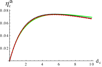
Figure 1: The correction of $O(\epsilon^{2})$ to $\eta_{c}$, $\eta_{c}^{\hbox{\scriptsize(2)}}$, as function of $d_{c}$ at the fixed point $P_{c}$. The solid line shows the prediction from the NPRG approach Coquand et al. (2018); the dashed line shows the two-loop/two-field result (present work); the dotted line shows the two-loop/efffective result (present work).

Concerning the fixed point $P_{5}$ we find – numerically – that it is, in fact marginally irrelevant – in agreement with the unstable character of $P_{c}$ and with the NPRG approach. However as said above there are difficulties to characterize $P_{5}$ – as well as $P_{c}$ – at low-temperatures. Indeed this implies to use the low-temperature variables $\overline{g}_{\lambda}=\overline{\lambda}\,\overline{\Delta}_{\kappa}$ and $\overline{g}_{\mu}=\overline{\mu}\,\overline{\Delta}_{\kappa}$ at order $\epsilon^{2}$. But, in the vicinity of $P_{5}$ – or $P_{c}$ – one has at next-to-leading order in $\epsilon$:

$$\overline{g}_{\mu}=\mathcal{C}_{\mu}^{(2)}\mathcal{C}_{\Delta_{\kappa}}^{(-1)}\epsilon+\mathcal{C}_{\mu}^{(3)}\mathcal{C}_{\Delta_{\kappa}}^{(-1)}\epsilon^{2}+\mathcal{C}_{\mu}^{(2)}\mathcal{C}_{\Delta_{\kappa}}^{(0)}\epsilon^{2}+O(\epsilon^{3})$$

where it appears that, due to the specific scaling of $\overline{\Delta}_{\kappa}$ with $\epsilon$ that involves negative powers of this parameter, the subsubleading contribution in $\epsilon$ to $\mu$ – $\mathcal{C}_{\mu}^{(3)}$ – is needed but is obviously lacking within the present – two-loop order – computation.

Conclusion

We have investigated quenched disordered membranes by means of a two-loop order perturbative approach. As a main result our approach clearly confirms the finding obtained with the NPRG approach Coquand et al. (2018), i.e. the existence of a richer phase diagram than that expected from previous investigations: the existence of a novel fixed point $P_{c}$ characterizing a wrinkling phase transition occurring at a temperature $T_{c}$ separating a disorder-free phase at $T>T_{c}$ controlled by the vanishing-disorder attractive fixed point $P_{4}$ and a low-temperature $T<T_{c}$ “glassy-phase” controlled by the vanishing-temperature, finite-disorder, attractive fixed point $P_{5}$. We thus have reached a consistent picture of disordered membranes at finite temperatures and in particular of the occurrence of a wrinkling transition. Our work reinforces the interest to investigate experimentally or numerically this transition in several systems involving both curvature and stretching disorder. This includes (i) a further study of partially polymerized fluid vesicles that have been already investigated by Chaieb et al. and have shown to be qualitatively and quantitatively well explained by the scenario proposed in Coquand et al. (2018); Coquand et al. (2020a) and (ii) a careful investigation of graphene and graphene-like materials with quenched lattice defects. Moreover our work, by confirming the attractive character of the vanishing temperature fixed point $P_{5}$, opens the possibility of a low-temperature phase controlled by a complex energy landscape and a genuine “glassy phase” that have been intensively looked for theoretically. It is thus pressing to probe this phase experimentally and numerically, notably in the context of the physics of graphene where it would be of prime interest to study the effects induced by disorder on the electronic and transport properties of graphene and graphene-like materials in this phase. Finally, from a more formal point of view our work strongly suggests to investigate deeply the nature of the perturbative series in the vicinity of the fixed points $P_{5}$ and $P_{c}$. In particular it would be of interest, even if it would represent a very substantial amount of work, to see whether the three-loop contributions indeed raise the ambiguities encountered within the two-loop order computation when studying the wrinkling transition.

Appendix A Renormalization group equations: two-field theory

One gives here the two-loop RG equations for the – dimensionless – coupling constants (forgetting their overlining) entering in action Eq.(4) :

$$\begin{split}\partial_{t}{\mu}&=-{\mu}\,\eta_{ut}+\frac{d_{c}\,{\mu}^{2}}{6(16\,\pi^{2})}(1+2{\Delta}_{\kappa})\\ &+\frac{d_{c}\,{\mu}^{2}\big{(}{\mu}(686{\Delta}_{\kappa}^{2}+908{\Delta}_{\kappa}+227)({\lambda}+{\mu})({\lambda}+2{\mu})-227{\Delta}_{\lambda}{\mu}^{2}(4{\Delta}_{\kappa}+1)-227{\Delta}_{\mu}(4{\Delta}_{\kappa}+1)({\lambda}^{2}+2{\lambda}{\mu}+2{\mu}^{2})\big{)}}{216(16\,\pi^{2})^{2}\,({\lambda}+2{\mu})^{2}}\,,\end{split}$$

$$\begin{split}\partial_{t}{\lambda}&=-{\lambda}\,\eta_{ut}+\frac{d_{c}\,(6{\lambda}^{2}+6{\lambda}{\mu}+{\mu}^{2})}{6(16\,\pi^{2})}(1+2{\Delta}_{\kappa})+\frac{d_{c}}{216(16\,\pi^{2})^{2}\,({\lambda}+2{\mu})^{2}}\bigg{[}{\mu}({\lambda}+2{\mu})\Big{(}-2{\Delta}_{\kappa}^{2}\big{(}108(d_{c}+9){\lambda}^{3}\\ &+18(16d_{c}+63){\lambda}^{2}{\mu}+(156d_{c}+239){\lambda}{\mu}^{2}+(24d_{c}+77){\mu}^{3}\big{)}-4{\Delta}_{\kappa}\big{(}54(d_{c}+7){\lambda}^{3}+72(2d_{c}+3){\lambda}^{2}{\mu}\\ &+(78d_{c}-179){\lambda}{\mu}^{2}+(12d_{c}-17){\mu}^{3}\big{)}-\big{(}54(d_{c}+7){\lambda}^{3}+72(2d_{c}+3){\lambda}^{2}{\mu}+(78d_{c}-179){\lambda}{\mu}^{2}+(12d_{c}-17){\mu}^{3}\big{)}\Big{)}\\ &+{\Delta}_{\lambda}{\mu}^{2}(4{\Delta}_{\kappa}+1)(378{\lambda}^{2}-162{\lambda}{\mu}-17{\mu}^{2})+{\Delta}_{\mu}(4{\Delta}_{\kappa}+1)(378{\lambda}^{4}+594{\lambda}^{3}{\mu}+415{\lambda}^{2}{\mu}^{2}-358{\lambda}{\mu}^{3}-34{\mu}^{4})\bigg{]}\,,\end{split}$$

$$\begin{split}\partial_{t}{\Delta}_{\mu}&=-{\Delta}_{\mu}\,\eta_{ut}+\frac{d_{c}\,{\mu}\,\big{(}2{\Delta}_{\mu}(2{\Delta}_{\kappa}+1)-{\Delta}_{\kappa}^{2}{\mu}\big{)}}{6(16\,\pi^{2})}+\frac{d_{c}\,{\mu}}{108\,(16\pi^{2})^{2}\,({\lambda}+2{\mu})^{2}}\bigg{[}{\Delta}_{\lambda}\big{(}343{\Delta}_{\kappa}^{2}{\mu}^{3}-227{\Delta}_{\mu}{\mu}^{2}(4{\Delta}_{\kappa}+1)\big{)}\\ &+{\Delta}_{\mu}{\mu}\big{(}343{\Delta}_{\kappa}^{2}(3{\lambda}^{2}+8{\lambda}{\mu}+6{\mu}^{2})+908{\Delta}_{\kappa}({\lambda}+{\mu})({\lambda}+2{\mu})+227({\lambda}+{\mu})({\lambda}+2{\mu})\big{)}\\ &-{\Delta}_{\kappa}^{2}{\mu}^{2}(232{\Delta}_{\kappa}+227)({\lambda}+{\mu})({\lambda}+2{\mu})-227{\Delta}_{\mu}^{2}(4{\Delta}_{\kappa}+1)({\lambda}^{2}+2{\lambda}{\mu}+2{\mu}^{2})\bigg{]}\,,\end{split}$$

$$\begin{split}\partial_{t}{\Delta}_{\lambda}&=-{\Delta}_{\lambda}\,\eta_{ut}-\frac{d_{c}\,{\Delta}_{\kappa}^{2}\,(6{\lambda}^{2}+6{\lambda}{\mu}+{\mu}^{2})}{6(16\,\pi^{2})}+\frac{2d_{c}\big{(}3{\Delta}_{\lambda}(2{\lambda}+{\mu})+{\Delta}_{\mu}(3{\lambda}+{\mu})\big{)}}{6(16\,\pi^{2})}(1+2{\Delta}_{\kappa})\\ &-\frac{d_{c}}{108\,(16\pi^{2})^{2}({\lambda}+2{\mu})^{2}}\bigg{[}{\Delta}_{\kappa}^{2}\Big{(}{\Delta}_{\lambda}{\mu}\big{(}216(d_{c}+9){\lambda}^{3}+18(52d_{c}+387){\lambda}^{2}{\mu}+72(16d_{c}+63){\lambda}{\mu}^{2}+(288d_{c}+401){\mu}^{3}\big{)}\\ &\>+{\Delta}_{\mu}\big{(}108(d_{c}+9){\lambda}^{4}+36(16d_{c}+63){\lambda}^{3}{\mu}+3(348d_{c}+995){\lambda}^{2}{\mu}^{2}+16(45d_{c}+79){\lambda}{\mu}^{3}+6(24d_{c}+77){\mu}^{4}\big{)}\Big{)}\\ &\>+(4{\Delta}_{\kappa}+1)({\lambda}+2{\mu})\Big{(}9d_{c}(3{\lambda}+{\mu})({\lambda}+2{\mu})\big{(}2{\Delta}_{\lambda}{\mu}+{\Delta}_{\mu}({\lambda}+{\mu})\big{)}+{\mu}({\lambda}+{\mu})\big{(}{\Delta}_{\lambda}(378{\lambda}-81{\mu})-{\Delta}_{\mu}(81{\lambda}+17{\mu})\big{)}\Big{)}\\ &\>+{\Delta}_{\kappa}^{2}{\mu}({\lambda}+2{\mu})\Big{(}-4{\Delta}_{\kappa}\big{(}27(d_{c}+11){\lambda}^{3}+9(8d_{c}+51){\lambda}^{2}{\mu}+(39d_{c}+209){\lambda}{\mu}^{2}+(6d_{c}+47){\mu}^{3}\big{)}\\ &\>-\big{(}54(d_{c}+7){\lambda}^{3}+72(2d_{c}+3){\lambda}^{2}{\mu}+(78d_{c}-179){\lambda}{\mu}^{2}+(12d_{c}-17){\mu}^{3}\big{)}\Big{)}\\ &\>-(4{\Delta}_{\kappa}+1)\big{(}{\Delta}_{\lambda}(378{\lambda}-81{\mu})-{\Delta}_{\mu}(81{\lambda}+17{\mu})\big{)}\big{(}{\Delta}_{\lambda}{\mu}^{2}+{\Delta}_{\mu}({\lambda}^{2}+2{\lambda}{\mu}+2{\mu}^{2})\big{)}\bigg{]}\,,\end{split}$$

$$\begin{split}\partial_{t}{\Delta}_{\kappa}&={\Delta}_{\kappa}\,\eta_{t}-\frac{5\,{\Delta}_{\kappa}\big{(}{\Delta}_{\lambda}{\mu}^{2}+{\Delta}_{\mu}({\lambda}^{2}+2{\lambda}{\mu}+2{\mu}^{2})\big{)}}{16\,\pi^{2}\,({\lambda}+2{\mu})^{2}}\\ &+\frac{{\Delta}_{\kappa}}{36(16\,\pi^{2})^{2}\,({\lambda}+2{\mu})^{4}}\bigg{[}-{\Delta}_{\kappa}^{2}{\mu}^{2}({\lambda}+2{\mu})^{2}\big{(}(39d_{c}+490){\lambda}^{2}+4(39d_{c}+110){\lambda}{\mu}+(81d_{c}+130){\mu}^{2}\big{)}\\ &+{\mu}({\lambda}+2{\mu})\bigg{(}5{\Delta}_{\lambda}{\mu}^{2}\big{(}3(15d_{c}+47){\Delta}_{\kappa}{\mu}+(15d_{c}+32){\mu}+411{\Delta}_{\kappa}{\lambda}+122{\lambda}\big{)}\\ &+{\Delta}_{\mu}\Big{(}{\lambda}^{3}\big{(}3(39d_{c}+415){\Delta}_{\kappa}+(39d_{c}+340)\big{)}+3{\lambda}^{2}{\mu}\big{(}234d_{c}{\Delta}_{\kappa}+78d_{c}+435{\Delta}_{\kappa}+70\big{)}\\ &+2{\lambda}{\mu}^{2}\big{(}(477d_{c}+600){\Delta}_{\kappa}+(159d_{c}+50)\big{)}+2{\mu}^{3}\big{(}3(81d_{c}+55){\Delta}_{\kappa}+(81d_{c}-20)\big{)}\Big{)}\bigg{)}\\ &+30{\mu}^{2}\big{(}-53{\Delta}_{\lambda}^{2}{\mu}^{2}-{\Delta}_{\lambda}{\Delta}_{\mu}(61{\lambda}^{2}+32{\lambda}{\mu}+32{\mu}^{2})\big{)}-30{\Delta\mu}^{2}\big{(}17{\lambda}^{4}+14{\lambda}^{3}{\mu}+10{\lambda}^{2}{\mu}^{2}-8{\lambda}{\mu}^{3}-4{\mu}^{4}\big{)}\bigg{]}\,,\end{split}$$

with

$$\begin{split}\eta_{t}&=\frac{5{\mu}\big{(}{\lambda}+{\mu})}{16\,\pi^{2}({\lambda}+2{\mu})}-\frac{5\Big{(}2{\Delta}_{\mu}({\lambda}^{2}+2{\lambda}{\mu}+2{\mu}^{2})-{\mu}\big{(}{\Delta}_{\kappa}({\lambda}^{2}+3{\lambda}{\mu}+2{\mu}^{2})-2{\Delta}_{\lambda}{\mu}\big{)}\Big{)}}{16\,\pi^{2}\,({\lambda}+2{\mu})^{2}}\\ &+\frac{{\mu}^{2}\big{(}(-39\,d_{c}-340){\lambda}^{2}-4(39\,d_{c}+35){\lambda}{\mu}+(20-81\,d_{c}){\mu}^{2}\big{)}}{72(16\,\pi^{2})^{2}\,({\lambda}+2{\mu})^{2}}\\ &-\frac{1}{72(16\,\pi^{2})^{2}\,({\lambda}+2{\mu})^{4}}\bigg{[}2({\lambda}+2{\mu})\bigg{(}{\mu}(2{\Delta}_{\kappa}+1)\Big{(}{\Delta}_{\mu}\big{(}(-39d_{c}-340){\lambda}^{3}-6(39d_{c}+35){\lambda}^{2}{\mu}-2(159d_{c}+50){\lambda}{\mu}^{2}\\ &+2(20-81d_{c}){\mu}^{3}\big{)}-5{\Delta}_{\lambda}{\mu}^{2}\big{(}(15d_{c}+32){\mu}+122{\lambda}\big{)}\Big{)}-2880\pi^{2}({\lambda}+2{\mu})\big{(}{\Delta}_{\lambda}{\mu}^{2}+{\Delta}_{\mu}({\lambda}^{2}+2{\lambda}{\mu}+2{\mu}^{2})\big{)}\bigg{)}\\ &+3{\Delta}_{\kappa}{\mu}^{2}({\lambda}+2{\mu})^{2}\Big{(}{\lambda}^{2}\big{(}39(d_{c}+10){\Delta}_{\kappa}+39d_{c}+340\big{)}+4{\lambda}{\mu}\big{(}(39d_{c}+60){\Delta}_{\kappa}+39d_{c}+35\big{)}\\ &+{\mu}^{2}\big{(}(81d_{c}+30){\Delta}_{\kappa}+81d_{c}-20\big{)}\Big{)}+20\Big{(}53{\Delta}_{\lambda}^{2}{\mu}^{4}+{\Delta}_{\lambda}{\Delta}_{\mu}{\mu}^{2}(61{\lambda}^{2}+32{\lambda}{\mu}+32{\mu}^{2})\\ &+{\Delta}_{\mu}^{2}(17{\lambda}^{4}+14{\lambda}^{3}{\mu}+10{\lambda}^{2}{\mu}^{2}-8{\lambda}{\mu}^{3}-4{\mu}^{4})\Big{)}\bigg{]}\end{split}$$

and $\eta_{ut}=\epsilon-2\eta_{t}\,.$

Appendix B Renormalization group equations: effective field theory

The effective field theory is obtained after an integration over the phonon field $\mathbf{u}$ in Eq.(4), see Coquand et al. (2020b):

$$\begin{split}&S_{\hbox{\scriptsize eff}}=\int_{\mathbf{k}}\frac{\widetilde{Z}_{\alpha\beta}}{2}k^{4}\,\mathbf{h}^{\alpha}(\mathbf{k}).\mathbf{h}^{\beta}(-\mathbf{k})\\ &+{1\over 4}\int_{\mathbf{k}_{1},\mathbf{k}_{2},\mathbf{k}_{3},\mathbf{k}_{4}}\!\!\!\!\!\!\!\!\!\!\!\!\!\!\!\!\!\!\!\!\!\!\mathbf{h}^{\alpha}(\mathbf{k}_{1}).\mathbf{h}^{\alpha}(\mathbf{k}_{2})\widetilde{R}^{ab,cd}_{\alpha\beta}(\mathbf{q})k_{1}^{a}\,k_{2}^{b}\,k_{3}^{c}\,k_{4}^{d}\,\mathbf{h}^{\beta}(\mathbf{k}_{3}).\mathbf{h}^{\beta}(\mathbf{k}_{4})\end{split}$$

where $\int_{\mathbf{k}}=\int{d^{D}k}/(2\pi^{D})$, $\mathbf{q}=\mathbf{k}_{1}+\mathbf{k}_{2}=-\mathbf{k}_{3}-\mathbf{k}_{4}$, and the interaction tensor $\widetilde{R}^{ab,cd}_{\alpha\beta}$ is defined as follows:

$$\widetilde{R}^{ab,cd}_{\alpha\beta}(\mathbf{q})=\widetilde{b}^{\alpha\beta}N_{ab,cd}(\mathbf{q})+\widetilde{\mu}^{\alpha\beta}M_{ab,cd}(\mathbf{q})\,.$$ (15)

In this expression the transverse tensors $N$ and $M$ are defined as a function of the projector transverse to $\mathbf{q}$, $P^{T}_{ab}=\delta_{ab}-q_{a}q_{b}/{\bf q}^{2}$, by:

$$\begin{split}&N_{ab,cd}(\mathbf{q})=\frac{1}{D-1}P^{T}_{ab}(\mathbf{q})P^{T}_{cd}(\mathbf{q})\\ &M_{ab,cd}(\mathbf{q})=\frac{1}{2}\big{[}P^{T}_{ac}(\mathbf{q})P^{T}_{bd}(\mathbf{q})+P^{T}_{ad}(\mathbf{q})P^{T}_{bc}(\mathbf{q})\big{]}-N_{ab,cd}(\mathbf{q})\,.\end{split}$$

Finally the coupling constant $\widetilde{b}_{\alpha\beta}=\widetilde{b}\,\delta_{\alpha\beta}-\widetilde{\Delta}_{b}\,J_{\alpha\beta}$ is related to the bare couplings $\widetilde{\mu}$, $\widetilde{\lambda}$, $\widetilde{\Delta}_{\mu}$ and $\widetilde{\Delta}_{\lambda}$ by:

$$\begin{split}&\widetilde{b}=\frac{\widetilde{\mu}(D\widetilde{\lambda}+2\widetilde{\mu})}{\widetilde{\lambda}+2\widetilde{\mu}}\\ &\widetilde{\Delta}_{b}=\frac{D(\widetilde{\Delta}_{\mu}\widetilde{\lambda}^{2}+2\widetilde{\Delta}_{\lambda}\widetilde{\mu}^{2})-2\widetilde{\mu}\big{(}\widetilde{\Delta}_{\lambda}\widetilde{\mu}-2\widetilde{\Delta}_{\mu}(\widetilde{\lambda}+\widetilde{\mu})\big{)}}{(\widetilde{\lambda}+2\widetilde{\mu})^{2}}\,.\end{split}$$

The two-loop RG equations are then given by:

$$\begin{split}\partial_{t}\mu&=-\mu\,\eta_{ut}+\frac{d_{c}\,\mu^{2}}{6(16\pi^{2})}(1+2\Delta_{\kappa})\\ &+\frac{d_{c}\,\mu^{2}}{1296(16\pi^{2})^{2}}\bigg{[}\mu(574+2296\Delta_{\kappa}+1732\Delta_{\kappa}^{2})+b(107+428\Delta_{\kappa}+326\Delta_{\kappa}^{2})-(574\Delta_{\mu}+107\Delta_{b})(1+4\Delta_{\kappa})\bigg{]}\,,\end{split}$$

$$\begin{split}\partial_{t}b&=-b\,\eta_{ut}+\frac{5\,d_{c}\,b^{2}}{12(16\pi^{2})}(1+2\Delta_{\kappa})\\ &-\frac{5\,d_{c}\,b^{2}}{2592(16\pi^{2})^{2}}\bigg{[}(178\Delta_{\mu}-91\Delta_{b})(1+4\Delta_{\kappa})+b(91+364\Delta_{\kappa}+394\Delta_{\kappa}^{2})-2\mu(89+356\Delta_{\kappa}+146\Delta_{\kappa}^{2})\bigg{]}\,,\end{split}$$

$$\begin{split}\partial_{t}\Delta_{\mu}&=-\Delta_{\mu}\,\eta_{ut}-\frac{d_{c}\,\mu\big{(}\mu\Delta_{\kappa}^{2}-2\Delta_{\mu}(1+2\Delta_{\kappa})\big{)}}{6(16\pi^{2})}\\ &-\frac{d_{c}\,\mu}{648(16\pi^{2})^{2}}\bigg{[}107\Delta_{b}\Delta_{\mu}(1+4\Delta_{\kappa})-b\Delta_{\mu}(107+428\Delta_{\kappa}+326\Delta_{\kappa}^{2})+574\Delta_{\mu}^{2}(1+4\Delta_{\kappa})-163\mu\,\Delta_{b}\,\Delta_{\kappa}^{2}\\ &+b\,\mu\,\Delta_{\kappa}^{2}(107+112\Delta_{\kappa})-2\mu\Delta_{\mu}(287+1148\Delta_{\kappa}+1299\Delta_{\kappa}^{2})+574\Delta_{\kappa}^{2}\mu^{2}+584\Delta_{\kappa}^{3}\mu^{2}\bigg{]}\,,\end{split}$$

$$\begin{split}\partial_{t}\Delta_{b}&=-\Delta_{b}\,\eta_{ut}-\frac{5\,d_{c}\,b\big{(}b\Delta_{\kappa}^{2}-2\Delta_{b}(1+2\Delta_{\kappa})\big{)}}{12(16\pi^{2})}\\ &-\frac{5d_{c}\,b}{1296(16\pi^{2})^{2}}\bigg{[}b^{2}\Delta_{\kappa}^{2}(91+212\Delta_{\kappa})-b\,\Delta_{b}(91+364\Delta_{\kappa}+591\Delta_{\kappa}^{2})+2b\,\Delta_{\kappa}^{2}\big{(}73\Delta_{\mu}+\mu(32\Delta_{\kappa}-89)\big{)}\\ &+\Delta_{b}\big{(}(91\Delta_{b}-178\Delta_{\mu})(1+4\Delta_{\kappa})+2\mu(89+356\Delta_{\kappa}+146\Delta_{\kappa}^{2})\big{)}\bigg{]}\,,\end{split}$$

$$\begin{split}\partial_{t}\Delta_{\kappa}&=\Delta_{\kappa}\,\eta_{t}-\frac{5(\Delta_{b}+2\Delta_{\mu})}{6(16\pi^{2})}\Delta_{\kappa}\\ &+\frac{\Delta_{\kappa}}{1296(16\pi^{2})^{2}}\bigg{[}5b^{2}(15d_{c}-242)\Delta_{\kappa}^{2}-2\Big{(}795\Delta_{b}^{2}-870\Delta_{b}\Delta_{\mu}-60\Delta_{\mu}^{2}+5\Delta_{b}\mu(58+129\Delta_{\kappa})\\ &-2\mu\,\Delta\mu\big{(}111d_{c}(1+3\Delta_{\kappa})+5(33\Delta_{\kappa}-4)\big{)}+2\mu^{2}\Delta_{\kappa}^{2}(130+111d_{c})\Big{)}\\ &-5b\Big{(}\Delta_{b}\big{(}15d_{c}(1+3\Delta_{\kappa})-212-681\Delta_{\kappa}\big{)}+2\big{(}\Delta_{\mu}(58+129\Delta_{\kappa})-56\mu\Delta_{\kappa}^{2}\big{)}\Big{)}\bigg{]}\,,\end{split}$$

with

$$\begin{split}\eta_{t}&=\frac{5(b+2\mu)}{6(16\pi^{2})}(1+\Delta_{\kappa})-\frac{5(\Delta_{b}+2\Delta_{\mu})}{6(16\pi^{2})}\\ &+\frac{1}{2592(16\pi^{2})^{2}}\bigg{[}-1060\Delta_{b}^{2}+5b^{2}\big{(}15d_{c}(1+3\Delta_{\kappa}+3\Delta_{\kappa}^{2})-2(106+318\Delta_{\kappa}+333\Delta_{\kappa}^{2})\big{)}+80\Delta_{\mu}^{2}\\ &+8\mu\Delta_{\mu}(1+2\Delta_{\kappa})(111d_{c}-20)-4\mu^{2}\big{(}111d_{c}(1+3\Delta_{\kappa}+3\Delta_{\kappa}^{2})+10(9\Delta_{\kappa}^{2}-6\Delta_{\kappa}-2)\big{)}\\ &+1160\Delta_{b}\big{(}\Delta_{\mu}-(1+2\Delta_{\kappa})\mu\big{)}-10b\big{(}\Delta_{b}(15d_{c}-212)(1+2\Delta_{\kappa})+116\Delta_{\mu}(1+2\Delta_{\kappa})-4\mu(29+87\Delta_{\kappa}+72\Delta_{\kappa}^{2})\big{)}\bigg{]}\end{split}$$

and $\eta_{ut}=\epsilon-2\eta_{t}\,.$

References

• Radzihovsky (2004) L. Radzihovsky, Proceedings of the Fifth Jerusalem Winter School for Theoretical Physics (World Scientific, Singapore, 2004).
• Dotsenko (2001) V. S. Dotsenko, Introduction to the Replica Theory of Disordered Statistical Systems (Cambridge University Press, Cambridge, 2001).
• Young (1998) A. P. Young, ed., Spin glasses and random fields (World Scientific, Singapore, 1998).
• T. Nattermann (1999) T. Nattermann, Spin Glasses and Random Fields (World Scientific, Singapore, 1999).
• De Dominicis et al. (1998) C. De Dominicis, I. Kondor, and T. Temesvari, Spin glasses and random fields (A. P. Young (Ed.), World Scientific, Singapore, 1998).
• De Dominicis and Giardina (2006) C. De Dominicis and I. Giardina, Random Fields And Spin Glasses: A Field Theory Approach (Cambridge University Press, Cambridge, 2006).
• K. J. Wiese and P. Le Doussal (2007) K. J. Wiese and P. Le Doussal, Markov Proc. Relat. Fields 13, 777 (2007).
• Tarjus and Tissier (2020) G. Tarjus and M. Tissier, Eur. Phys. J. B 93, 50 (2020).
• M. Mutz, D. Bensimon, and M. J. Brienne (1991) M. Mutz, D. Bensimon, and M. J. Brienne, Phys. Rev. Lett. 67, 923 (1991).
• S. Chaieb, V.K. Natrajan, and A. A. El-rahman (2006) S. Chaieb, V.K. Natrajan, and A. A. El-rahman, Phys. Rev. Lett. 96, 078101 (2006).
• Chaieb et al. (2008) S. Chaieb, S. Málková, and J. Lal, J. Theor. Biol. 251, 60 (2008).
• Radzihovsky and D. R. Nelson (1991) L. Radzihovsky and D. R. Nelson, Phys. Rev. A 44, 3525 (1991).
• Banhart et al. (2011) F. Banhart, J. Kotakoski, and A. Krasheninnikov, ACS Nano 5, 26 (2011).
• Liu et al. (2015) L. Liu, M. Qing, Y. Wang, and S. Chen, J. Mater. Sci. Technol. 31, 599 (2015).
• G. Yang, L. Li, W. B. Lee and M.C. Ng (2018) G. Yang, L. Li, W. B. Lee and M.C. Ng, Sci. Technol. Adv. Mater. 19, 613 (2018).
• B. Ni, T. Zhang, J. Li, X. Li and H. Gao (2019) B. Ni, T. Zhang, J. Li, X. Li and H. Gao, Handbook of Graphene: Physics, Chemistry, and Biology (John Wiley and Sons, 2019), vol. 2.
• Novoselov et al. (2004) K. S. Novoselov, A. K. Geim, S. V. Morozov, D. Jiang, Y. Zhang, S. V. Dubonos, I. V. Gregorieva, and A. A. Firsov, Science 306, 666 (2004).
• Novoselov et al. (2005) K. S. Novoselov, A. K. Geim, S. V. Morozov, D. Jiang, M. I. Katsnelson, I. V. Gregorieva, S. V. Dubonos, and A. A. Firsov, Nature (London) 438, 197 (2005).
• J. Kotakoski, A.V. Krasheninnikov, U. Kaiser and J.C. Meyer (2011) J. Kotakoski, A.V. Krasheninnikov, U. Kaiser and J.C. Meyer, Phys. Rev. Lett. 106, 105505 (2011).
• F.R. Eder, J. Kotakoski, U. Kaiser and J.C. Meyer (2014) F.R. Eder, J. Kotakoski, U. Kaiser and J.C. Meyer, Scientific Reports 4, 4060 (2014).
• W.-J. Joo et al (2017) W.-J. Joo et al, Science Advances 3, e1601821 (2017).
• Nelson and Radzihovsky (1991) D. R. Nelson and L. Radzihovsky, Europhys. Lett. 16, 79 (1991).
• Radzihovsky and P. Le Doussal (1992) L. Radzihovsky and P. Le Doussal, J. Phys. I France 2, 599 (1992).
• D. C. Morse, T. C. Lubensky and G. S. Grest (1992) D. C. Morse, T. C. Lubensky and G. S. Grest, Phys. Rev. A 45, R2151 (1992).
• D. C. Morse and T. C. Lubensky (1992) D. C. Morse and T. C. Lubensky, Phys. Rev. A 46, 1751 (1992).
• Bensimon et al. (1992) D. Bensimon, D. Mukamel, and L. Peliti, Europhys. Lett. 18, 269 (1992).
• Bensimon et al. (1993) D. Bensimon, M. Mutz, and T. Gulik, Physica A 194, 190 (1993).
• R. Attal, S. Chaieb, and D. Bensimon (1993) R. Attal, S. Chaieb, and D. Bensimon, Phys. Rev. E 48, 2232 (1993).
• Park and Kwon (1996) Y. Park and C. Kwon, Phys. Rev. E 54, 3032 (1996).
• Mori (1996) S. Mori, Phys. Rev. E 54, 338 (1996).
• Benyoussef et al. (1998) A. Benyoussef, D. Dohmi, A. E. Kenz, and L. Peliti, Eur. Phys. J. B 6, 503 (1998).
• Le Doussal and Radzihovsky (1993) P. Le Doussal and L. Radzihovsky, Phys. Rev. B 48, 3548 (1993).
• Mori and Wadati (1994) S. Mori and M. Wadati, Phys. Lett. A 185, 206 (1994).
• P. Le Doussal and L. Radzihovsky (2018) P. Le Doussal and L. Radzihovsky, Ann. Phys. (N.Y.) 392, 340 (2018).
• J.-P. Kownacki and Mouhanna (2009) J.-P. Kownacki and D. Mouhanna, Phys. Rev. E 79, 040101(R) (2009).
• F. L. Braghin and N. Hasselmann (2010) F. L. Braghin and N. Hasselmann, Phys. Rev. B 82, 035407 (2010).
• Essafi et al. (2011) K. Essafi, J.-P. Kownacki, and D. Mouhanna, Phys. Rev. Lett. 106, 128102 (2011).
• N. Hasselmann and F. L. Braghin (2011) N. Hasselmann and F. L. Braghin, Phys. Rev. E 83, 031137 (2011).
• Essafi et al. (2014) K. Essafi, J.-P. Kownacki, and D. Mouhanna, Phys. Rev. E 89, 042101 (2014).
• Coquand and Mouhanna (2016) O. Coquand and D. Mouhanna, Phys. Rev. E 94, 032125 (2016).
• Coquand et al. (2018) O. Coquand, K. Essafi, J.-P. Kownacki, and D. Mouhanna, Phys. Rev E 97, 030102(R) (2018).
• Coquand et al. (2020a) O. Coquand, K. Essafi, J.-P. Kownacki, and D. Mouhanna, Phys. Rev. E 101, 042602 (2020a).
• D. R. Saykin, V. Yu. Kachorovskii and I. S. Burmistrov (2020) D. R. Saykin, V. Yu. Kachorovskii and I. S. Burmistrov, Phys. Rev. Research. 2 (2020).
• Coquand et al. (2020b) O. Coquand, D. Mouhanna, and S. Teber, Phys. Rev. E 101, 062104 (2020b).
• A. Mauri and M.I. Katsnelson (2020) A. Mauri and M.I. Katsnelson, Nucl. Phys. B 956, 115040 (2020).
• Guitter et al. (1988) E. Guitter, F. David, S. Leibler, and L. Peliti, Phys. Rev. Lett. 61, 2949 (1988).
• Guitter et al. (1989) E. Guitter, F. David, S. Leibler, and L. Peliti, J. Phys. (Paris) 50, 1787 (1989).
• Kotikov and Teber (2019) A. V. Kotikov and S. Teber, Phys. Part. Nucl. 50, 1 (2019).
• Coquand and Mouhanna (2020) O. Coquand and D. Mouhanna, unpublished (2020).
• Nelson and Peliti (1987) D. R. Nelson and L. Peliti, J. Phys. (Paris) 48, 1085 (1987).