Dynamics and control of entangled electron-photon states in nanophotonic systems with time-variable parameters

Abstract

We study the dynamics of strongly coupled nanophotonic systems with time-variable parameters. The approximate analytic solutions are obtained for a broad class of open quantum systems including a two-level fermion emitter strongly coupled to a multimode quantized electromagnetic field in a cavity with time-varying cavity resonances or the electron transition energy. The coupling of the fermion and photon subsystems to their dissipative reservoirs is included within the stochastic equation of evolution approach, which is equivalent to the Lindblad approximation in the master equation formalism. The analytic solutions for the quantum states and the observables are obtained under the approximation that the rate of parameter modulation and the amplitude of the frequency modulation are much smaller than the optical transition frequencies. At the same time, they can be arbitrary with respect to the generalized Rabi oscillations frequency which determines the coherent dynamics. Therefore, our analytic theory can be applied to an arbitrary modulation of the parameters, both slower and faster than the Rabi frequency, for complete control of the quantum state. In particular, we demonstrate protocols for switching on and off the entanglement between the fermionic and photonic degrees of freedom, swapping between the quantum states, and the decoupling of the fermionic qubit from the cavity field due to modulation-induced transparency.

I Introduction

Solid-state photonic qubits based on the fermion systems coupled to a quantized electromagnetic (EM) field in a plasmonic or dielectric nanocavity are promising for a variety of quantum information and quantum sensing applications haroche ; lodahl2015 ; degen2017 . Their benefits include compatibility with semiconductor technology, scalability, and potential for operation at temperatures much higher than the alternative platforms based on superconducting qubits or trapped ions. Indeed, strong coupling to single quantum emitters in dielectric nanocavities was demonstrated in various systems, for example color centers lukin2016 or quantum dots (QDs) Refs. deppe ; reithmaier . In plasmonic cavities, strong coupling to single molecules Refs. chikkaraddy2016 ; benz2016 ; park2016 and colloidal QDs pelton2018 ; gross2018 ; park2019 has been achieved at room temperature; see, e.g., Refs. lodahl2015 ; thorma2015 ; bitton2019 ; kono2019 ; may2020 for recent reviews.

While the quantum dynamics of entangled nanophotonic systems is interesting by itself, many applications would benefit from to control and modify the qubit states by time-dependent variation of certain parameters, while taking into account various processes of decoherence and dissipation. There is of course a large body of work related to cavity quantum electrodynamics (QED) with time-variable parameters. For example, the dynamics of nanophotonics systems with periodic modulation of some parameter, such as the cavity size or the position of a quantum emitter in a cavity, has been studied extensively in the burgeoning fields of cavity optomechanics aspelmeyer2014 ; meystre2013 ; pirkkalainen2015 and quantum acoustics chu2017 ; hong2017 ; arriola2019 . In this case the most interesting new element added to the nanophotonic system is the parametric resonance or the dressing of the electron-photon coupling by mechanical oscillations. Near the parametric resonance, the system can be mapped to an exactly solvable time-independent Hamiltonian within the rotating-wave approximation tokman2020 .

There is a class of time-dependent Hamiltonians for which the nonstationary Schrödinger equation can be solved exactly in the analytic form, notably multistate Landau-Zener Hamiltonians and driven Tavis-Cummings Hamiltonians sinitsyn2018 ; chernyak2018 ; see also li2018 where this technique was applied to the quantum annealing problem. Here we are interested in the nanophotonic applications, so we have to consider open multimode photonic systems with an arbitrary time dependence of the parameters. Therefore, we restrict ourselves to the adiabatic dynamics, for which the analytic solution can be found for a broad variety of systems with time-dependent cavity or fermion emitter parameters, and with dissipation included at the level of the Lindblad formalism. We find that the condition of adiabaticity is not that restrictive; in particular it still allows one to consider the parameter variation at a rate comparable to or faster than the generalized Rabi frequency in strongly coupled systems, which may be required for qubit manipulation.

We will also stick to the rotating wave approximation (RWA) Scully1997 . The use of RWA restricts the coupling strength to the values much lower than the characteristic energies in the system, such as the optical transition or photon energy. The emerging studies of the so-called ultra-strong coupling regime kono2019 have to go beyond the RWA. Nevertheless, for the vast majority of experiments, including nonperturbative strong coupling dynamics and entanglement, the RWA is adequate and provides some crucial simplifications that allow one to obtain analytic solutions.

In particular, within Schrödinger’s description, the equations of motion for the components of an infinitely dimensional state vector $\left|\Psi\right\rangle$ that describes a coupled fermion-boson system can be split into the blocks of low dimensions if the RWA is applied. This is true even if the dynamics of the fermion subsystem is nonperturbative, e.g. the effects of saturation are important. Note that there is no such simplification in the Heisenberg representation, except within the perturbation theory; see e.g. Scully1997 . This is because boson operators are defined on a basis of infinite dimension and truncation of their dynamics into blocks of small dimensions is generally not possible (see also tokman2020 ). The Schrödinger’s approach also leads to fewer equations for the state vector components than the approach based on the von Neumann master equation for the elements of the density matrix. This is especially true for a system with many degrees of freedom, e.g., many electron states coupled to multiple boson field modes.

Obviously, the Schrödinger equation in its standard form cannot be applied to describe open systems coupled to a dissipative reservoir. In this case the stochastic versions of the equation of evolution for the state vector have been developed, e.g. the method of quantum jumps Scully1997 ; Plenio1998 . This method is optimal for numerical analysis in the Monte-Carlo type schemes. Here we formulate the stochastic equation which is more conducive to the analytic treatment. In tokman2020 we showed that the stochastic equation of evolution for the state vector can be derived directly from the Heisenberg-Langevin formalism.

The paper is structured as follows. Section II formulates the model and the Hamiltonian for two-level electron system and a quantized EM field in a nanocavity with time-variable parameters. It treats a single-mode cavity in detail as a particular case and describes simple manipulations with a single cavity mode coupled to a single fermionic qubit. Section III considers the dynamics of two time-modulated cavity modes coupled to a single quantum emitter and Sec. IV treats the case of a variable frequency of the optical transition in a fermion qubit. Section V solves the quantum dynamics for an open time-dependent system with the coupling to dissipative reservoirs taken into account. An interesting phenomenon of modulation-induced transparency is analyzed. Numerical estimations for various nanophotonic systems reported in the literature are presented. Conclusions are in Section VI. Appendix A describes the quantization procedure for a plasmon cavity field with strongly subwavelength localization. Appendix B summarizes the main properties of the stochastic equation of evolution and compares with the Lindblad density-matrix formalism.

II Cavity QED with time-variable parameters

II.1 Standard cavity QED Hamiltonian for a quantized field coupled to a two-level emitter

For reference, we start from summarizing basic textbook facts about a quantized electron system resonantly coupled to the quantum multimode EM field of a nanocavity without any time dependence, and then consider the time-dependent models in the next sections.

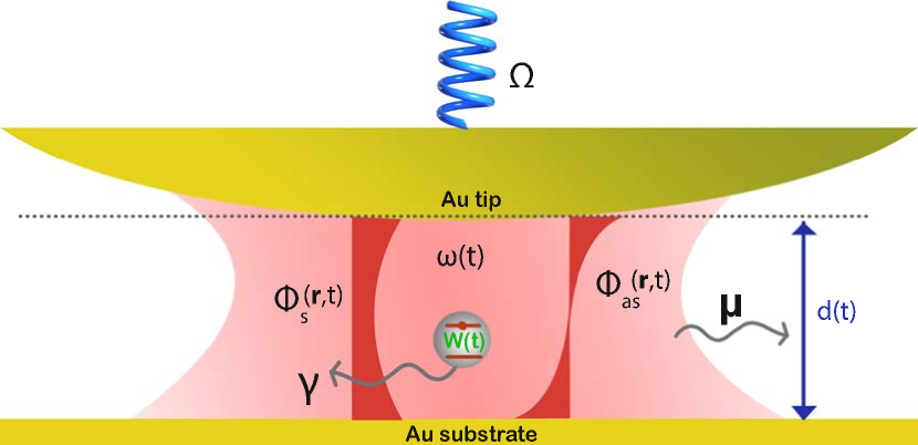
(a)

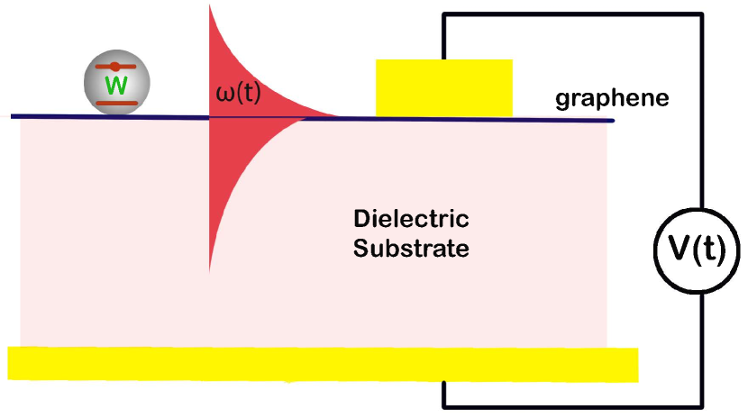
(b)

Figure 1: (a) A sketch of a quantum emitter (e.g. a quantum dot or a single molecule) in a nanocavity with time-dependent parameters created by a metallic nanotip of the scanning probe and a metallic substrate. The profiles of the electric potential $\Phi\left(\mathbf{r},t\right)$ for the symmetric and antisymmetric mode (see Appendix A) are sketched. Other parameters are the transition energy $W(t)$ for a quantum emitter, the optical field frequency $\omega(t)$, the cavity height $d(t)$, and the relaxation constants of the cavity field, $\mu$, and a quantum emitter, $\gamma$. (b) A quantum emitter coupled to the cavity surface plasmon field supported by graphene. The mode frequency $\omega(t)$ can be varied by applying variable voltage $V(t)$ which modifies the charge density in graphene.

Consider the simplest version of the fermion subsystem: two electron states $\left|0\right\rangle$ and $\left|1\right\rangle$ with energies $0$ and $W$, respectively. We will call it an “atom” for brevity, although it can be electron states of a molecule, a quantum dot, a defect in a semiconductor, or any other electron system. Introduce creation and annihilation operators of the excited state $\left|1\right\rangle$, $\hat{\sigma}=\left|0\right\rangle\left\langle 1\right|$, $\hat{\sigma}^{\dagger}=\left|1\right\rangle\left\langle 0\right|$, which satisfy standard commutation relations for fermions:

$$\hat{\sigma}^{\dagger}\left|0\right\rangle=\left|1\right\rangle,\hat{\sigma}\left|1\right\rangle=\left|0\right\rangle,\hat{\sigma}\hat{\sigma}=\hat{\sigma}^{\dagger}\hat{\sigma}^{\dagger}=0;\left[\hat{\sigma},\hat{\sigma}^{\dagger}\right]_{+}=\hat{\sigma}\hat{\sigma}^{\dagger}+\hat{\sigma}^{\dagger}\hat{\sigma}=1.$$

The Hamiltonian of an atom is

$$\hat{H}_{a}=W\hat{\sigma}^{\dagger}\hat{\sigma}.$$ (1)

We will also need the dipole moment operator, $\mathbf{\hat{d}}=\mathbf{d}\left(\hat{\sigma}^{\dagger}+\hat{\sigma}\right)$, where $\mathbf{d=}\left\langle 1\right|\mathbf{\hat{d}}\left|0\right\rangle$ is a real vector. For a finite motion we can always choose the coordinate representation of stationary states in terms of real functions.

We assume that an atom is placed in a nanocavity and is resonantly coupled to the electric field of quantized cavity modes. Figure 1 sketches two out of many possible geometries of a time-variable nanocavity, e.g. formed by the nanotip of the scanning probe and the metallic substrate (Fig. 1a), similar to the recent experiments with strong coupling to single quantum emitters park2016 ; pelton2018 ; gross2018 ; park2019 . Of course many other cavity geometries are possible, such as the one in Fig. 1b where the quantum emitter is coupled to the cavity surface plasmon field supported by graphene. Here the optical transition energy $W(t)$, the photon mode frequency $\omega(t)$, and field amplitudes described by an electric potential $\Phi\left(\mathbf{r},t\right)$ are all subject to external modulation by e.g. varying the tip distance to the substrate, the position of a quantum emitter in a cavity, or a variable voltage applied to graphene or to a QD in a semiconductor nanostructure, but we will start from the Hamiltonian without any time dependence for future comparison.

We use a standard representation for the electric field operator in a cavity:

$$\mathbf{\hat{E}}=\sum_{i}\left[\mathbf{E}_{i}\left(\mathbf{r}\right)\hat{c}_{i}+\mathbf{E}_{i}^{\ast}\left(\mathbf{r}\right)\hat{c}_{i}^{\dagger}\right],$$ (2)

where $\hat{c}_{i}^{\dagger},\hat{c}_{i}$ are creation and annihilation operators for photons at frequency $\omega_{i}$; the functions $\mathbf{E}_{i}\left(\mathbf{r}\right)$ describe the spatial structure of the EM modes in a cavity. The relation between the modal frequency $\omega_{i}$ and the function $\mathbf{E}_{i}\left(\mathbf{r}\right)$ can be found by solving the boundary-value problem of the classical electrodynamics Scully1997 . The normalization conditions Tokman2016

$$\int_{V}\frac{\partial\left[\omega_{i}^{2}\varepsilon\left(\omega_{i},\mathbf{r}\right)\right]}{\omega_{i}\partial\omega_{i}}\mathbf{E}_{i}^{\ast}\left(\mathbf{r}\right)\mathbf{E}_{i}\left(\mathbf{r}\right)d^{3}r=4\pi\hbar\omega_{i}$$ (3)

ensure correct bosonic commutators $\left[\hat{c}_{i},\hat{c}_{i}^{\dagger}\right]=\delta_{ij}$ and the field Hamiltonian in the form

$$\hat{H}_{em}=\hbar\sum_{i}\omega_{i}\left(\hat{c}_{i}^{\dagger}\hat{c}_{i}+\frac{1}{2}\right).$$ (4)

Here $V$ is a quantization volume and $\varepsilon\left(\omega,\mathbf{r}\right)$ is the dielectric function of a dispersive medium that fills the cavity.

Equation (3) is true for any fields satisfying Maxwell’s equations as long as intracavity losses can be neglected and the flux of the Poynting vector through the total cavity surface is zero; see, e.g., Refs. Tokman2016 ; Tokman2013 ; Tokman2015 ; Tokman2018 . Of course the photon losses are always important when calculating the decoherence rates and fluctuations. What matters for Eq. (3) is that the effect of losses on the spatial structure of the cavity modes is insignificant. The latter is true as long as it makes sense to talk about cavity modes at all, which means in practice that the cavity Q-factor is at least around 10 or greater.

In many experiments involving strong coupling to a single quantum emitter the plasmonic cavities of nanometer size and even below 1 nm are used. The quantization procedure for a strongly subwavelength plasmon field has its peculiarities. We describe it in detail in Appendix A.

Adding the interaction Hamiltonian with a EM cavity mode in the electric dipole approximation, $-\mathbf{\hat{d}}\cdot\mathbf{\hat{E}}$, the Hamiltonian of an atom coupled to a single mode EM field is

$$\hat{H}=\hat{H}_{em}+\hat{H}_{a}-\mathbf{d}\left(\hat{\sigma}^{\dagger}+\hat{\sigma}\right)\cdot\left[\mathbf{E}\left(\mathbf{r}\right)\hat{c}+\mathbf{E}^{\ast}\left(\mathbf{r}\right)\hat{c}^{\dagger}\right]_{\mathbf{r}=\mathbf{r}_{a}},$$ (5)

where $\mathbf{r}=\mathbf{r}_{a}$ denotes the position of an atom inside the cavity. This can be rewritten as

$$\hat{H} = \hat{H}_{em}+\hat{H}_{a}-\left(\chi\hat{\sigma}^{\dagger}\hat{c}+\chi^{\ast}\hat{\sigma}\hat{c}^{\dagger}+\chi\hat{\sigma}\hat{c}+\chi^{\ast}\hat{\sigma}^{\dagger}\hat{c}^{\dagger}\right)$$ (6)

where $\chi=\left(\mathbf{d}\cdot\mathbf{E}\right)_{\mathbf{r}=\mathbf{r}_{a}}$.

The best conditions for entanglement are realized in the vicinity of an atom-field resonance, where one can apply the rotating wave approximation (RWA). The RWA Hamiltonian is obtained by dropping the last two terms in Eq. (6). Note that we can always take the functions $\mathbf{E}\left(\mathbf{r}\right)$ to be real at the position of an atom. This single-mode model is of course the Jaynes-Cummings Hamiltonian JC1963 .

II.2 Quantized electromagnetic field in a time-variable cavity

In a standard approach to quantization of the EM field based on Eqs. (2)-(4), a set of mode frequencies $\omega_{i}$ and the relation between the frequency $\omega_{i}$ and the spatial structure of the field mode $\mathbf{E}_{i}\left(\mathbf{r}\right)$ are determined by solving the boundary-value problem for the classical EM field. Let’s assume that the solution of this boundary-value problem depends on a certain parameter $p$, for example the cavity height $d(t)$ in Fig. 1 or the position of the emitter with respect to the field distribution. In this case $\omega_{i}(p)$ and $\mathbf{E}_{i}\left(\mathbf{r,}p\right)$ are functions of $p$. Of course the solution depends on many parameters of the cavity, but we consider the situation when this particular parameter is adiabatically changing with time. As usual, “adiabatically” means that the change can be arbitrary (e.g. periodic or not) but it should be slow as compared to typical frequencies of all subsystems when the parameters are constant, such as the modal frequencies and the transition frequency of a quantum emitter. It is important that the rate of change of parameters can be arbitrary as compared to characteristic frequency scales which determine the interaction between subsystems, such as the Rabi frequency, as long as these scales are smaller than the modal or transition frequencies kruskal1962 ; tokman2011 .

For an adiabatically varying parameter Eqs. (2)-(4) depend on the instantaneous value of the parameter,

$$\mathbf{\hat{E}}=\sum_{i}\left[\mathbf{E}_{i}\left(\mathbf{r,}p\right)\hat{c}_{i}+\mathbf{E}_{i}^{\ast}\left(\mathbf{r,}p\right)\hat{c}_{i}^{\dagger}\right],$$ (7)

$$\hat{H}\ =\sum_{i}\hat{H}_{i}\ \ \ \hat{H}_{i}=\hbar\omega_{i}(p)\left(\hat{c}_{i}^{\dagger}\hat{c}_{i}+\frac{1}{2}\right),$$ (8)

$$\int_{V\left(p\right)}\frac{\partial\left[\omega_{i}^{2}\varepsilon\left(\omega_{i},\mathbf{r}\right)\right]}{\omega_{i}\partial\omega_{i}}\mathbf{E}_{i}^{\ast}\left(\mathbf{r,}p\right)\mathbf{E}_{i}\left(\mathbf{r,}p\right)d^{3}r=4\pi\hbar\omega_{i}(p).$$ (9)

The solution of the Schrödinger equation $i\hbar\frac{\partial}{\partial t}\left|\Psi_{i}\right\rangle=\hat{H}_{i}\left|\Psi_{i}\right\rangle$ for a given field mode is

$$\left|\Psi_{i}\right\rangle=\sum_{n=0}^{\infty}C_{n}\left|n\right\rangle$$ (10)

where $C_{n}=C_{n}^{0}e^{-i(n+\frac{1}{2})\int_{0}^{t}\omega_{i}\left(\tau\right)d\tau}$, $\omega_{i}\left(t\right)\equiv$ $\omega_{i}\left(p\left(t\right)\right)$, and $\left|n\right\rangle$ are Fock states. For a bosonic field described by a standard quantized harmonic oscillator, if we choose the coordinate representation expressed via Hermite polynomials, the parameters of the polynomials will be time-dependent. One can easily see that the above solution conserves the adiabatic invariant $\frac{\left\langle\Psi_{i}\right|\hat{H}_{i}\left|\Psi_{i}\right\rangle}{\omega_{i}\left(t\right)}$ , just like in a classical slowly time-varying harmonic oscillator problem LL1 .

II.3 Quantum emitter coupled to a quantized EM field with a time-variable amplitude

Let a two-level electron system (an atom) be located at the point $\mathbf{r}=\mathbf{0}$ inside the cavity. The Hamiltonian of the system including the coupling of an atom to a particular cavity mode and its adiabatic modulation can be described within the RWA,

$$\hat{H}=\hbar\omega(t)\left(\hat{c}^{\dagger}\hat{c}+\frac{1}{2}\right)+W\hat{\sigma}^{\dagger}\hat{\sigma}-\left[\mathbf{d}\cdot\mathbf{E}\left(t\right)\hat{\sigma}^{\dagger}\hat{c}+\mathbf{d}^{\ast}\cdot\mathbf{E}^{\ast}\left(t\right)\hat{\sigma}\hat{c}^{\dagger}\right],$$ (11)

where $\mathbf{E}\left(\mathbf{0},t\right)=\mathbf{E}\left(t\right)$. The time dependence of the field amplitude follows from the parameter modulation.

The wave function of the coupled photon-electron state can be written as

$$\Psi=\sum_{n=0}^{\infty}\left(C_{n0}\left|n\right\rangle\left|0\right\rangle+C_{n1}\left|n\right\rangle\left|1\right\rangle\right),$$ (12)

where we will maintain the same order, $\left|photon\right\rangle\left|fermion\right\rangle$ of the state products everywhere. Substituting it in the Schrödinger equation and taking into account the time variation of the parameter, we obtain the equation for the ground energy state,

$$\dot{C}_{00}+i\omega_{00}\left(t\right)C_{00}=0,$$ (13)

and a pair of equations for “resonant” states,

$$\dot{C}_{n0}+i\omega_{n0}\left(t\right)C_{n0}-i\Omega_{R}^{\ast}\left(t\right)C_{\left(n-1\right)1}=0,$$ (14)

$$\dot{C}_{\left(n-1\right)1}+i\omega_{\left(n-1\right)1}\left(t\right)C_{\left(n-1\right)1}-i\Omega_{R}\left(t\right)C_{n0}=0,$$ (15)

where

$$\omega_{n0}\left(t\right)=\omega\left(t\right)\left(n+\frac{1}{2}\right),\ \ \omega_{n1}\left(t\right)=\omega_{n0}\left(t\right)+\frac{W}{\hbar},\ \ \Omega_{R}\left(t\right)=\frac{\mathbf{d\cdot E}\left(t\right)}{\hbar}\sqrt{n}.$$

Equations (14), (15) can be written in a more convenient form after making a substitution

$$\left(\begin{array}[]{c}C_{n0}\\ C_{\left(n-1\right)1}\end{array}\right)=\left(\begin{array}[]{c}G_{n0}e^{-i\int_{0}^{t}\omega_{n0}\left(\tau\right)d\tau}\\ G_{\left(n-1\right)1}e^{-i\int_{0}^{t}\omega_{\left(n-1\right)1}\left(\tau\right)d\tau}\end{array}\right),$$ (16)

which gives

$$\dot{G}_{n0}-i\Omega_{R}^{\ast}\left(t\right)e^{i\int_{0}^{t}\delta\left(\tau\right)d\tau}G_{\left(n-1\right)1}=0,$$ (17)

$$\dot{G}_{\left(n-1\right)1}-i\Omega_{R}\left(t\right)e^{-i\int_{0}^{t}\delta\left(\tau\right)d\tau}G_{n0}=0,$$ (18)

where $\delta\left(t\right)=\omega\left(t\right)-\frac{W}{\hbar}$.

When there is no modulation, i.e. $\delta$, $\omega$, and $\Omega_{R}$ are constant, Eqs. (17), (18) have a simple solution $G_{(n-1)1},G_{n0}\propto e^{-i\nu t}$, where the eigenvalues are

$$\nu_{1,2}=\frac{\delta}{2}\pm\sqrt{\frac{\delta^{2}}{4}+|\Omega_{R}|^{2}},$$ (19)

and the eigenvectors satisfy

$$K_{1,2}=\left[\frac{G_{n0}}{G_{(n-1)1}}\right]_{1,2}=\frac{\nu_{1,2}e^{i\delta t}}{\Omega_{R}},$$ (20)

where $K_{1}K_{2}^{\ast}=-1$. The eigenvalues $\nu_{1,2}$ as a function of detuning $\delta$ are shown in Fig. 2. It is easy to verify that in the region $\delta\ll-|\Omega_{R}|$ the eigenvalue $\nu_{1}$ corresponds to the dominant state $\left|n-1\right\rangle\left|1\right\rangle$, whereas in the region $\delta\gg|\Omega_{R}|$ this eigenvalue corresponds to dominant state $\left|n\right\rangle\left|0\right\rangle$. For the eigenvalue $\nu_{2}$ it is exactly the opposite.

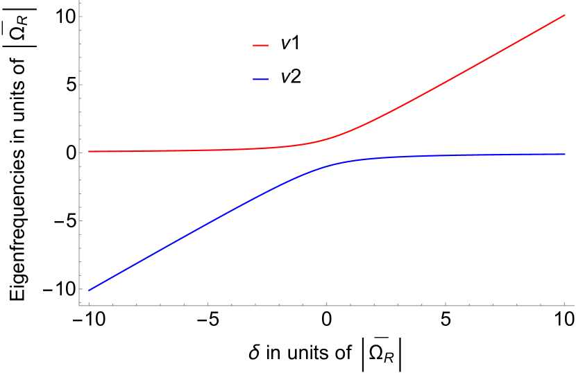
(a)

Figure 2: Frequency eigenvalues $\nu_{1,2}$ from Eq. (19) as a function of detuning $\delta$ from the resonance, $\delta=\omega-\frac{W}{\hbar}$. All frequencies are in units of the average Rabi frequency $\overline{\Omega_{R}}$.

When a cavity parameter is modulated, for example, a cavity height $d(t)$ in Fig. 1, both frequencies and field amplitudes $\mathbf{E}_{i}\left(\mathbf{r,}p\right)$ get modulated; see Eq. (9). Therefore, the Rabi frequency $\Omega_{R}$ gets modulated. For a periodic modulation, the function $\Omega_{R}\left(t\right)e^{-i\int_{0}^{t}\delta\left(\tau\right)d\tau}$ is periodic and can be expanded in the Fourier series,

$$\Omega_{R}\left(t\right)e^{-i\int_{0}^{t}\delta\left(\tau\right)d\tau}=\sum_{n=-\infty}^{\infty}R_{n}e^{-in\Omega t},$$ (21)

where $\Omega$ is the modulation frequency. The explicit expressions for the Fourier amplitudes $R_{n}$ can be obtained for any specific model of a cavity; see, e.g., Appendix A for the plasmonic cavity, which shows specific examples of the cavity mode frequencies, field amplitudes, and their modulation.

When the modulation frequency and amplitude of the eigenmode frequencies are small enough, one can neglect the modulation of the Rabi frequency in Eqs. (17), (18). This corresponds to the WKB approximation and one can see it by taking the time derivative of Eq. (18):

$$\frac{d^{2}G_{\left(n-1\right)1}}{dt^{2}}+\left(i\delta\left(t\right)-\frac{1}{\Omega_{R}\left(t\right)}\frac{d\Omega_{R}}{dt}\right)\frac{dG_{\left(n-1\right)1}}{dt}+\left|\Omega_{R}\left(t\right)\right|^{2}G_{\left(n-1\right)1}=0.$$ (22)

Now we can estimate the order of magnitude of different terms in Eq. (22). Assume that the cavity mode frequency is modulated as $\omega_{i}(t)=\bar{\omega}+\delta(t)$. Since Eq. (9) defines a certain dependence $\Omega_{R}(\omega_{i})$, one can estimate $\left|\frac{\Omega_{R}^{-1}\dot{\Omega}_{R}}{\delta}\right|\sim\left|\frac{\dot{\delta}}{\Omega_{R}\delta}\frac{d\Omega_{R}}{d\omega_{i}}\right|_{\omega_{i}=\bar{\omega}}$ and $\left|\Omega_{R}-\overline{\Omega_{R}}\right|\sim\left|\frac{d\Omega_{R}}{d\omega_{i}}\delta\right|$. For estimations we take $\frac{d\Omega_{R}}{d\omega_{i}}\sim\frac{\overline{\Omega_{R}}}{\bar{\omega}}$, $\delta\sim\Delta\omega$, and $\dot{\delta}\sim\Omega\Delta\omega$ where $\overline{\Omega_{R}}=\Omega_{R}(\bar{\omega})$ and $\Delta\omega$ is the frequency change over the time $\Omega^{-1}$. This gives $\left|\frac{\Omega_{R}^{-1}\dot{\Omega}_{R}}{\delta}\right|\sim\frac{\Omega}{\bar{\omega}}$ and $\left|\Omega_{R}-\overline{\Omega_{R}}\right|\sim\overline{\Omega_{R}}\frac{\Delta\omega}{\bar{\omega}}$. If $\Delta\omega,\Omega\ll\bar{\omega}$, Eq. (22) becomes

$$\frac{d^{2}G_{\left(n-1\right)1}}{dt^{2}}+i\delta\left(t\right)\frac{dG_{\left(n-1\right)1}}{dt}+\left|\overline{\Omega_{R}}\right|^{2}G_{\left(n-1\right)1}=0.$$ (23)

Equation (23) corresponds to the set of Eqs. (14), (15) with $\Omega_{R}=$ const $=\overline{\Omega_{R}}$.

If we consider for definiteness a sinusoidal modulation of the frequency of a given mode, $\omega\left(t\right)=\bar{\omega}-\Delta\omega\cdot\sin\left(\Omega t\right)$, and take into account that $\Delta\omega,\Omega,\overline{\Omega_{R}}\ll\overline{\omega}$, the Fourier amplitudes in Eq. (21) can be expressed through the Bessel functions,

$$R_{0}=\overline{\Omega_{R}}J_{0}\left(\frac{\Delta\omega}{\Omega}\right),\;R_{n}=(-i)^{|n|}\overline{\Omega_{R}}J_{|n|}\left(\frac{\Delta\omega}{\Omega}\right).$$ (24)

The decoherence processes can be added within the stochastic equation of evolution for the state vector, which is derived in Appendix B. However, we postpone doing this until we consider a more complex case of two quantized modes interacting with a quantum emitter.

II.4 Simple manipulations with a qubit coupled to a single-mode field

A single emitter coupled to a single-mode field in a time-variable cavity permits simple manipulations: a slow or fast sweep through the resonance $\omega(t)=W/\hbar$, bringing an electron-photon system in and out of entanglement by changing the values of coefficients in Eq. (12), transduction of the excitation between an atom and the EM field, e.g., between $\left|0\right\rangle\left|1\right\rangle$ and $\left|1\right\rangle\left|0\right\rangle$ states, etc.

Note that the rate of modulation or parameter variation has to be slow only as compared to the optical frequency. It does not have to be slow as compared to the average Rabi frequency $\overline{\Omega_{R}}$. Therefore, in the strong coupling regime a desired switching can be completed faster than the Rabi oscillations and decoherence rates.

Let’s look at some of these control operations in more detail. The sweep through resonance can be calculated exactly for each specific time dependence $\delta(t)$, but the limiting cases are well understood from the vast amount of literature on the linear coupling of the optical modes, Landau-Zener-type problems, etc kruskal1962 ; tokman2011 ; kochar1983 ; hallin1995 ; yokomizo2014 .

For a slow sweep, $\left|\frac{d\delta}{dt}\right|\ll\overline{|\Omega_{R}|^{2}}$, the system will follow each eigenvalue branch plotted in Fig. 2 without jumping between them: for example, if the system starts from $\nu_{1}$ at $\delta\ll-\overline{|\Omega_{R}|}$, it will stay on $\nu_{1}$ as it moves through resonance to $\delta\gg\overline{|\Omega_{R}|}$. This means that the quantum state of the system will be switched from $\left|n-1\right\rangle\left|1\right\rangle$ to $\left|n\right\rangle\left|0\right\rangle$.

In the opposite limit of a fast sweep, $\left|\frac{d\delta}{dt}\right|\gg\overline{|\Omega_{R}|^{2}}$, as the system moves through resonance from $\delta\ll-\overline{|\Omega_{R}|}$ to $\delta\gg\overline{|\Omega_{R}|}$ it jumps from one eigenvalue branch to another. As a result, the quantum state stays unchanged.

In the intermediate region $\left|\frac{d\delta}{dt}\right|\sim\overline{|\Omega_{R}|^{2}}$, by varying the sweep rate or the Rabi frequency $\overline{|\Omega_{R}|}$ one can get any desired combination of the quantum states at the output. In particular, for linear variation of the detuning, $\delta(t)=\beta t$ where $\beta$ is a constant, one can obtain an exact analytic solution of Eq. (23) to predict the evolution of the system:

$$G_{(n-1)1}(t)=\displaystyle e^{-\frac{i\beta t^{2}}{4}}\left[c_{1}D_{i\frac{\overline{|\Omega_{R}|}^{2}}{\beta}}\left(\sqrt{\beta}e^{-\frac{i\pi}{4}}t\right)+c_{2}D_{-i\frac{\overline{|\Omega_{R}|}^{2}}{\beta}-1}\left(i\sqrt{\beta}e^{-\frac{i\pi}{4}}t\right)\right],$$ (25)

where $D_{\nu}$ are the parabolic cylinder functions bateman and $c_{1,2}$ are arbitrary constants determined by initial conditions. This solution can be used, for example, to calculate the efficiency of the $\left|n-1\right\rangle\left|1\right\rangle$ quantum state tunneling, i.e., the probability of the transition from the top to bottom branch in Fig. 2 as the detuning $\delta(t)$ varies from $-\infty$ to $+\infty$:

$$\left|C_{(n-1)1}\right|_{\delta\rightarrow\infty}^{2}\approx\displaystyle e^{-\frac{\overline{2\pi|\Omega_{R}|}^{2}}{\beta}}\left|C_{(n-1)1}\right|_{\delta\rightarrow-\infty}^{2}.$$

As expected, the probability is approaching 1 when $\left|\frac{d\delta}{dt}\right|=\beta\gg\overline{|\Omega_{R}|}^{2}$ and becomes exponentially small in the opposite limit.

III Dynamics of two modulated cavity modes coupled to a quantum emitter

In order to perform more complex operations on the photonic qubits and get more functionality, we need to add one more quantized degree of freedom to the system. Here we consider two cavity modes in a time-variable cavity,

$$\mathbf{\hat{E}}=\mathbf{E}_{a}\left(\mathbf{r,}t\right)\hat{a}+\mathbf{E}_{a}^{\ast}\left(\mathbf{r,}t\right)\hat{a}^{\dagger}+\mathbf{E}_{b}\left(\mathbf{r,}t\right)\hat{b}+\mathbf{E}_{b}^{\ast}\left(\mathbf{r,}t\right)\hat{b}^{\dagger}.$$ (26)

We assume that the modulation of both frequencies has a small amplitude and average frequencies of both modes $\bar{\omega}_{a,b}$ are close to the transition frequency. In this case the RWA Hamiltonian for an atom + field system is

$$\hat{H}=\hbar\omega_{a}\left(t\right)\left(\hat{a}^{\dagger}\hat{a}+\frac{1}{2}\right)+\hbar\omega_{b}\left(t\right)\left(\hat{b}^{\dagger}\hat{b}+\frac{1}{2}\right)+W\hat{\sigma}^{\dagger}\hat{\sigma}-\left[\hat{\sigma}^{\dagger}\left(\chi_{a}\hat{a}+\chi_{b}\hat{b}\right)+\hat{\sigma}\left(\chi_{a}^{\ast}\hat{a}^{\dagger}+\chi_{b}^{\ast}\hat{b}^{\dagger}\right)\right],$$ (27)

where $\chi_{a,b}\left(t\right)=\mathbf{d\cdot E}_{a,b}\left(t\right)$.

The Schrödinger equation can be solved analytically within the RWA tokman2020 . As a simple example, we include only the transitions between the states with lowest energies, namely $\left|0_{a}\right\rangle\left|0_{b}\right\rangle\left|0\right\rangle,\left|0_{a}\right\rangle\left|0_{b}\right\rangle\left|1\right\rangle,\left|1_{a}\right\rangle\left|0_{b}\right\rangle\left|0\right\rangle,\left|0_{a}\right\rangle\left|1_{b}\right\rangle\left|0\right\rangle$, i.e. we seek the solution in the form

$$\Psi=C_{000}\left|0_{a}\right\rangle\left|0_{b}\right\rangle\left|0\right\rangle+C_{001}\left|0_{a}\right\rangle\left|0_{b}\right\rangle\left|1\right\rangle+C_{100}\left|1_{a}\right\rangle\left|0_{b}\right\rangle\left|0\right\rangle+C_{010}\left|0_{a}\right\rangle\left|1_{b}\right\rangle\left|0\right\rangle.$$ (28)

For arbitrary coefficients $C$ the state (28) is a tripartite entangled state which can be reduced to standard GHZ states by local operations dur2000 ; cunha2020 , e.g. by rotations on the Bloch sphere of each qubit. In most cases discussed in the literature the GHZ states are made of identical subsystems, e.g., photons shalm2012 ; agusti2020 . In our case the subsystems are of different nature: a fermionic electron system and bosonic EM field modes. This makes their rotations more complicated, but on the other hand, enables other interesting applications. For example, one can determine the statistics of atomic excitations by measuring the statistics of photons, or change the entangled state of coupled photon modes by changing the atomic state with a classical control field.

Similarly to tokman2020 , the equations for the coefficients are

$$\dot{C}_{000}+i\frac{\omega_{a}\left(t\right)+\omega_{b}\left(t\right)}{2}C_{000}=0;$$ (29)

$$\dot{C}_{001}+i\left(\frac{1}{2}\omega_{a}\left(t\right)+\frac{1}{2}\omega_{b}\left(t\right)+\frac{W}{\hbar}\right)C_{001}-i\Omega_{Ra}(t)C_{100}-i\Omega_{Rb}(t)C_{010}=0,$$ (30)

$$\dot{C}_{100}+i\left(\frac{3}{2}\omega_{a}\left(t\right)+\frac{1}{2}\omega_{b}\left(t\right)\right)C_{100}-i\Omega_{Ra}^{\ast}(t)C_{001}=0,$$ (31)

$$\dot{C}_{010}+i\left(\frac{1}{2}\omega_{a}\left(t\right)+\frac{3}{2}\omega_{b}\left(t\right)\right)C_{010}-i\Omega_{Rb}^{\ast}(t)C_{001}=0,$$ (32)

where $\Omega_{Ra,b}=\frac{\chi_{a,b}}{\hbar}$. Making the substitution

$$\left(\begin{array}[]{c}C_{001}\\ C_{100}\\ C_{010}\end{array}\right)=\left(\begin{array}[]{c}G_{0}\exp\left[-i\int_{0}^{t}\left(\frac{1}{2}\omega_{a}\left(\tau\right)+\frac{1}{2}\omega_{b}\left(\tau\right)+\frac{W}{\hbar}\right)d\tau\right]\\ G_{a}\exp\left[-i\int_{0}^{t}\left(\frac{3}{2}\omega_{a}\left(\tau\right)+\frac{1}{2}\omega_{b}\left(\tau\right)\right)d\tau\right]\\ G_{b}\exp\left[-i\int_{0}^{t}\left(\frac{1}{2}\omega_{a}\left(\tau\right)+\frac{3}{2}\omega_{b}\left(\tau\right)\right)d\tau\right]\end{array}\right),$$ (33)

we obtain

$$\dot{G}_{0}-i\Omega_{Ra}(t)G_{a}\exp\left[-i\int_{0}^{t}\left(\omega_{a}\left(\tau\right)-\frac{W}{\hbar}\right)d\tau\right]-i\Omega_{Rb}(t)G_{b}\exp\left[-i\int_{0}^{t}\left(\omega_{b}\left(\tau\right)-\frac{W}{\hbar}\right)d\tau\right]=0,$$ (34)

$$\dot{G}_{a}-i\Omega_{Ra}^{\ast}(t)G_{0}\exp\left[i\int_{0}^{t}\left(\omega_{a}\left(\tau\right)-\frac{W}{\hbar}\right)d\tau\right]=0,$$ (35)

$$\dot{G}_{b}-i\Omega_{Rb}^{\ast}(t)G_{0}\exp\left[i\int_{0}^{t}\left(\omega_{b}\left(\tau\right)-\frac{W}{\hbar}\right)d\tau\right]=0,$$ (36)

In Fig. 3, we show the eigenstates of the system described by Eqs. (30), (31) and (32) as a function of frequency detuning defined as $\omega_{a}-W/\hbar$. Here we assumed that $\Omega_{Ra}=\Omega_{Rb}\equiv\Omega_{R}$ and kept the difference $\omega_{b}-\omega_{a}=5\Omega_{R}$ constant, which can be achieved either by varying $W/\hbar$ while keeping constant $\omega_{a,b}$ or by varying $\omega_{a}$ and $\omega_{b}$ at the same rate while keeping $W/\hbar$ constant. The anticrossings are clearly seen in the plot of eigenfrequencies, when either $\omega_{a}$ or $\omega_{b}$ is resonant with the optical transition of an atom. As compared to Fig. 2, Fig. 3(b) shows more possibilities for switching between the three product states as the detuning is swept through the two resonances at the rate slower than the Rabi frequencies and the generation of both bipartite and tripartite entangled states in the vicinity of resonances if the sweeping rate is comparable to the Rabi frequencies.

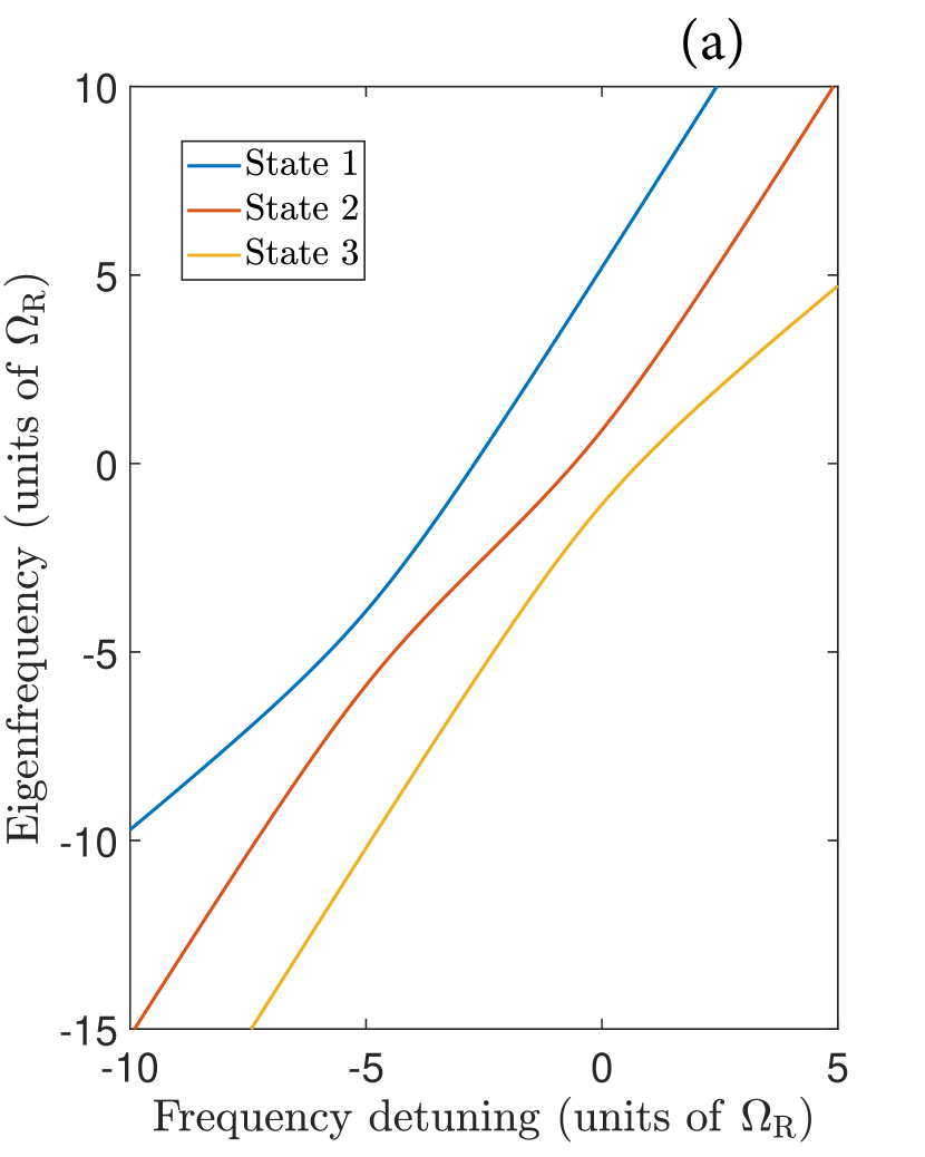
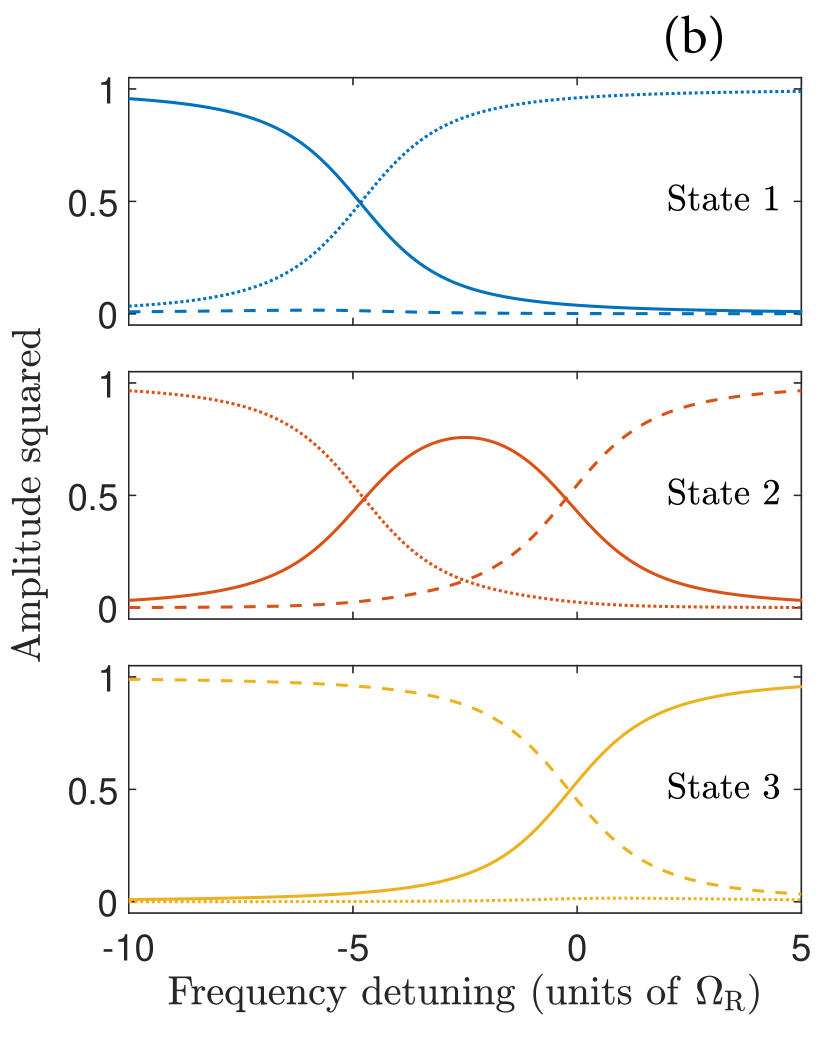
Figure 3: The eigenstates of the system described by Eqs. (30), (31) and (32) as a function of frequency detuning defined as $\omega_{a}-W/\hbar$, whereas the difference of modal frequencies $\omega_{b}-\omega_{a}=5\Omega_{R}$ is kept constant. The eigenfrequencies are shown in (a), and the amplitudes of the eigenstates are shown in (b), in which the amplitudes of $C_{001}$, $C_{100}$ and $C_{010}$ are represented by the solid, dashed and dotted lines, respectively. The eigenfrequencies are shifted by $\left.\left(\frac{1}{2}\omega_{a}+\frac{1}{2}\omega_{b}+\frac{W}{\hbar}\right)\right|_{\omega_{a}=W/\hbar}$.

Since the functions $\omega_{a,b}(t)$ and $\Omega_{a,b}$ are periodic with period $2\pi/\Omega$, we can use the expansion (21) in Eqs. (34)-(36).

If we keep only the resonant terms, assuming for example the following resonances, $\bar{\omega}_{a}=\frac{W}{\hbar}$ and $\bar{\omega}_{b}+m\Omega=\frac{W}{\hbar}$, where $m$ is the number of a particular Fourier harmonic, the equations get simplified,

$$\frac{d}{dt}\left(\begin{array}[]{c}G_{0}\\ G_{a}\\ G_{b}\end{array}\right)+\left(\begin{array}[]{ccc}0&-iR_{a0}&-iR_{bm}\\ -iR_{a0}^{\ast}&0&0\\ -iR_{bm}^{\ast}&0&0\end{array}\right)\left(\begin{array}[]{c}G_{0}\\ G_{a}\\ G_{b}\end{array}\right)=0.$$ (37)

Other (nonresonant) harmonics can be neglected only if $\Omega_{Ra,b}\ll\Omega$, see tokman2020 . When the modulation amplitude is zero, $R_{a0}=\Omega_{Ra}$ and $R_{bm}=0$. In this case one of the eigenvalues $\Gamma_{0}$ corresponds to the decoupled state $\left|0_{a}\right\rangle\left|1_{b}\right\rangle\left|0\right\rangle$. Two other eigenvalues $\Gamma_{1,2}$ describe the solution with Rabi oscillations between states $\left|0_{a}\right\rangle\left|0_{b}\right\rangle\left|1\right\rangle$ and $\left|1_{a}\right\rangle\left|0_{b}\right\rangle\left|0\right\rangle$.This is an obvious limit since frequency $\omega_{a}$ is in resonance with the transition frequency, whereas $\omega_{b}$ is out of resonance.

Assuming a sinusoidal modulation of the partial frequencies of both cavity modes as an example,

$$\omega_{a,b}\left(t\right)=\bar{\omega}_{a,b}-\Delta\omega_{a,b}\cdot\sin\left(\Omega t\right),$$ (38)

and using the well-known expansion in series of the harmonics of the modulation frequency $\Omega$, with coefficients expressed in terms of Bessel functions,

$$e^{-i\frac{\Delta\omega}{\Omega}\cos\left(\Omega t\right)}=J_{0}\left(\frac{\Delta\omega}{\Omega}\right)+2\sum_{n=1}^{\infty}\left(-i\right)^{n}J_{n}\left(\frac{\Delta\omega}{\Omega}\right)\cos\left(n\Omega t\right),$$ (39)

we can express Fourier amplitudes in Eq. (37) through Bessel functions:

$$R_{a0}=\overline{\Omega_{Ra}}J_{0}\left(\frac{\Delta\omega_{a}}{\Omega}\right),\;R_{bm}=(-i)^{|m|}\overline{\Omega_{Rb}}J_{|m|}\left(\frac{\Delta\omega_{b}}{\Omega}\right).$$ (40)

Note that the modulation amplitudes in Eq. (38) can be of the order of the modulation frequency, $\frac{\Delta\omega_{a,b}}{\Omega}\sim 1$, despite the requirement $\Delta\omega_{a,b}\ll$ $\bar{\omega}_{a,b}$.

As usual, to solve Eq. (37) one has to find the eigenvalues $\Gamma_{0,1,2}$ and eigenvectors of the matrix of coefficients. The characteristic equation for the eigenvalues is $\Gamma\left(\Gamma^{2}+\Omega_{R\Sigma}^{2}\right)=0$, where the cumulative Rabi frequency is

$$\Omega_{R\Sigma}=\sqrt{|R_{a0}|^{2}+|R_{bm}|^{2}}.$$ (41)

The result is

$$\Gamma_{0}=0,\ \Gamma_{1,2}=\pm i\Omega_{R\Sigma}.$$ (42)

Figure 4 shows one example of the cumulative Rabi frequency $\Omega_{R\Sigma}$ as a function of $\Delta\omega=\Delta\omega_{a}=\Delta\omega_{b}$ for $m=1$ and $\Omega_{Ra}=\Omega_{Rb}$. As expected, $\Omega_{R\Sigma}$ decays with detuning from resonances but the decay is nonmonotonic and depends on the order of harmonic resonances.

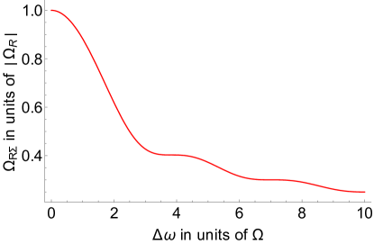
Figure 4: Cumulative Rabi frequency $\Omega_{R\Sigma}$ as a function of $\Delta\omega=\Delta\omega_{a}=\Delta\omega_{b}$ for $m=1$ and $\Omega_{R}=\Omega_{Ra}=\Omega_{Rb}$.

The eigenvalue $\Gamma_{0}$ (i.e. the solution $\propto e^{-\Gamma_{0}t}$ ) corresponds to the eigenvector $\left(\begin{array}[]{c}0\\ 1\\ -\frac{R_{a0}}{R_{bm}}\end{array}\right)$, whereas eigenvalues $\Gamma_{1,2}$ (i.e. the solution behaving as $\propto e^{-\Gamma_{1,2}t}$) correspond to the eigenvectors $\left(\begin{array}[]{c}\frac{\pm\Omega_{R\Sigma}}{R_{a0}^{\ast}}\\ 1\\ \frac{R_{bm}^{\ast}}{R_{a0}^{\ast}}.\end{array}\right)$. Here the eigenvectors are not normalized to $1$. The resulting solution is

$$\left(\begin{array}[]{c}G_{0}\\ G_{a}\\ G_{b}\end{array}\right)=A\left(\begin{array}[]{c}0\\ 1\\ -\frac{R_{a0}}{R_{bm}}\end{array}\right)+Be^{-i\Omega_{R\Sigma}t}\left(\begin{array}[]{c}\frac{\Omega_{R\Sigma}}{R_{a0}^{\ast}}\\ 1\\ \frac{R_{bm}^{\ast}}{R_{a0}^{\ast}}.\end{array}\right)+Ce^{i\Omega_{R\Sigma}t}\left(\begin{array}[]{c}\frac{-\Omega_{R\Sigma}}{R_{a0}^{\ast}}\\ 1\\ \frac{R_{bm}^{\ast}}{R_{a0}^{\ast}}.\end{array}\right),$$ (43)

where the constants $A$, $B$ and $C$ are determined by the initial conditions.

For an arbitrary initial state vector

$$\Psi=C_{000}(0)\left|0_{a}\right\rangle\left|0_{b}\right\rangle\left|0\right\rangle+C_{001}(0)\left|0_{a}\right\rangle\left|0_{b}\right\rangle\left|1\right\rangle+C_{100}(0)\left|1_{a}\right\rangle\left|0_{b}\right\rangle\left|0\right\rangle+C_{010}(0)\left|0_{a}\right\rangle\left|1_{b}\right\rangle\left|0\right\rangle,$$ (44)

satisfying the normalization condition

$$|C_{000}(0)|^{2}+|C_{001}(0)|^{2}+|C_{100}(0)|^{2}+|C_{010}(0)|^{2}=1,$$

the constants in Eq. (43) are

$$A=\frac{C_{100}(0)\frac{|R_{bm}|^{2}}{|R_{a0}|^{2}}-C_{010}(0)\frac{R_{bm}}{R_{a0}}}{1+\frac{|R_{bm}|^{2}}{|R_{a0}|^{2}}},$$

$$B=\frac{1}{2}\left(\frac{C_{100}(0)+C_{010}(0)\frac{R_{bm}}{R_{a0}}}{1+\frac{|R_{bm}|^{2}}{|R_{a0}|^{2}}}+C_{001}(0)\frac{R_{a0}^{\ast}}{\Omega_{R\Sigma}}\right),$$

$$C=\frac{1}{2}\left(\frac{C_{100}(0)+C_{010}(0)\frac{R_{bm}}{R_{a0}}}{1+\frac{|R_{bm}|^{2}}{|R_{a0}|^{2}}}-C_{001}(0)\frac{R_{a0}^{\ast}}{\Omega_{R\Sigma}}\right).$$ (45)

Let’s consider some examples of the initial conditions to illustrate this solution.

III.1 An atom is excited; both modes are in the vacuum state:

The initial state vector is $\Psi(0)=\left|0_{a}\right\rangle\left|0_{b}\right\rangle\left|1\right\rangle$. In this case Eq. (45) gives $A=0,B=-C=\frac{R_{a0}^{\ast}}{2\Omega_{R\Sigma}}$. The full expression for the state vector at any moment of time becomes

$$\Psi = e^{-i\int_{0}^{t}\omega_{001}\left(\tau\right)d\tau}\cos\left(\Omega_{R\Sigma}t\right)\left|0_{a}\right\rangle\left|0_{b}\right\rangle\left|1\right\rangle-i\frac{R_{a0}^{\ast}}{\Omega_{R\Sigma}}e^{-i\int_{0}^{t}\omega_{100}\left(\tau\right)d\tau}\sin\left(\Omega_{R\Sigma}t\right)\left|1_{a}\right\rangle\left|0_{b}\right\rangle\left|0\right\rangle$$ (46)

$$-i\frac{R_{bm}^{\ast}}{\Omega_{R\Sigma}}e^{-i\int_{0}^{t}\omega_{010}\left(\tau\right)d\tau}\sin\left(\Omega_{R\Sigma}t\right)\left|0_{a}\right\rangle\left|1_{b}\right\rangle\left|0\right\rangle,$$

where

$$\omega_{001}\left(t\right)=\frac{1}{2}\omega_{a}\left(t\right)+\frac{1}{2}\omega_{b}\left(t\right)+\frac{W}{\hbar},\ \ \omega_{100}\left(t\right)=\frac{3}{2}\omega_{a}\left(t\right)+\frac{1}{2}\omega_{b}\left(t\right),\ \ \ \ \omega_{010}\left(t\right)=\frac{1}{2}\omega_{a}\left(t\right)+\frac{3}{2}\omega_{b}\left(t\right).$$

As we see, an initial atomic excitation decays into a pair of electromagnetic modes. Their frequencies are modulated due to the modulation of the cavity geometry and are split by the cumulative Rabi frequency. In the absence of dissipation the excitation energy oscillates back and forth between an atom and the field modes at the cumulative Rabi frequency.

III.2 Both cavity modes are excited; the atom is in the ground state:

The initial state vector is $\Psi(0)=C_{100}(0)\left|1_{a}\right\rangle\left|0_{b}\right\rangle\left|0\right\rangle+C_{010}(0)\left|0_{a}\right\rangle\left|1_{b}\right\rangle\left|0\right\rangle$. In this case the state vector is

$$\Psi = -2iB\frac{\Omega_{R\Sigma}}{R_{a0}^{\ast}}e^{-i\int_{0}^{t}\omega_{001}\left(\tau\right)d\tau}\sin\left(\Omega_{R\Sigma}t\right)\left|0_{a}\right\rangle\left|0_{b}\right\rangle\left|1\right\rangle+\left(A+2B\cos\left(\Omega_{R\Sigma}t\right)\right)e^{-i\int_{0}^{t}\omega_{100}\left(\tau\right)d\tau}\left|1_{a}\right\rangle\left|0_{b}\right\rangle\left|0\right\rangle$$ (47)

$$+\left(2B\frac{R_{bm}^{\ast}}{R_{a0}^{\ast}}\cos\left(\Omega_{R\Sigma}t\right)-A\frac{R_{a0}}{R_{bm}}\right)e^{-i\int_{0}^{t}\omega_{010}\left(\tau\right)d\tau}\left|0_{a}\right\rangle\left|1_{b}\right\rangle\left|0\right\rangle,$$

where

$$A=\frac{C_{100}(0)\frac{|R_{bm}|^{2}}{|R_{a0}|^{2}}-C_{010}(0)\frac{R_{bm}}{R_{a0}}}{1+\frac{|R_{bm}|^{2}}{|R_{a0}|^{2}}},\;B=C=\frac{1}{2}\frac{C_{100}(0)+C_{010}(0)\frac{R_{bm}}{R_{a0}}}{1+\frac{|R_{bm}|^{2}}{|R_{a0}|^{2}}}.$$ (48)

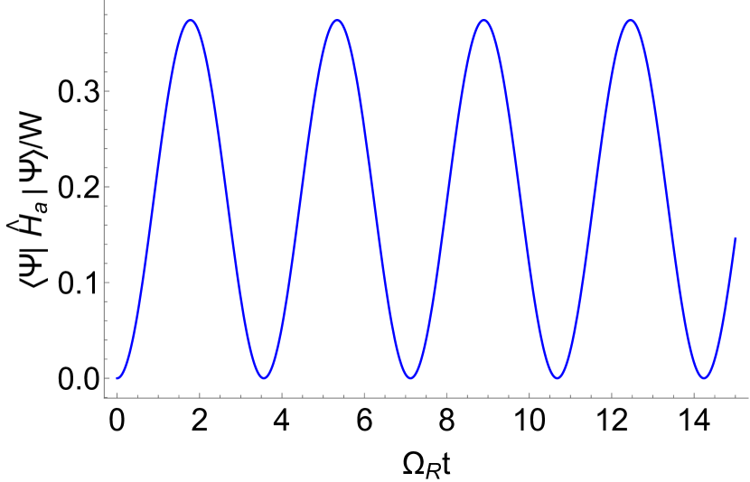
(a)

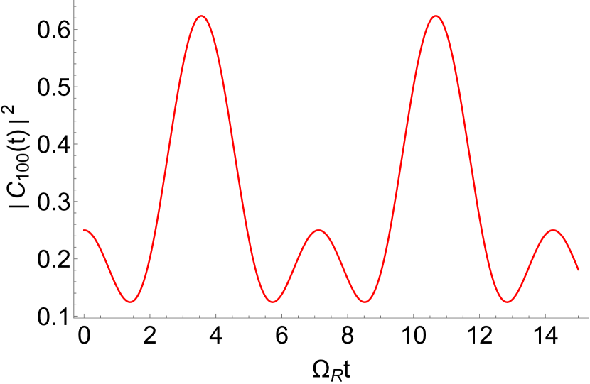
(b)

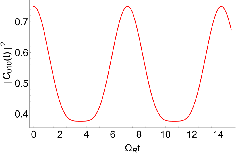
(c)

Figure 5: (a) The average normalized energy of an atom, (b) the number of quanta in mode $a$, and (c) the number of quanta in mode $b$ as a function of normalized time. The initial conditions are $C_{000}(0)=0$, $C_{001}(0)=0$, $C_{100}(0)=1/2$, and $C_{001}(0)=\sqrt{3}/2$; i.e., the two modes are initially excited with different amplitudes whereas an atom is in the ground state. Other parameters are $\Delta\omega_{a}=\Delta\omega_{b}=\Omega$, $m=1$, and $\Omega_{Ra}=\Omega_{Rb}=\Omega_{R}$.

An atom, originally in its ground state, will get excited through resonant coupling to the EM field, as is obvious from Eq. (47). The resulting dynamics of the averaged normalized energy of an atom $\left\langle\Psi\right|\hat{H}_{a}\left|\Psi\right\rangle/W$ and the numbers of quanta in mode $a$, $|C_{100}(t)|^{2}$ and mode $b$, $|C_{100}(t)|^{2}$ is shown in Fig. 5 for one generic set of initial conditions. Due to the presence of three coupled degrees of freedom, the evolution is more complicated than single-sinusoidal Rabi oscillations. Moreover, there is one particular choice of initial conditions, $C_{010}(0)=-C_{100}(0)\frac{R_{a0}}{R_{bm}}$, which corresponds to $B=C=0$ and $A=C_{100}(0)$, where the normalization condition gives $|C_{100}(0)|^{2}=\left(1+\frac{|R_{a0}|^{2}}{|R_{bm}|^{2}}\right)^{-1}$. This gives the following state vector,

$$\left(\begin{array}[]{c}C_{001}\\ C_{100}\\ C_{010}\end{array}\right)=C_{100}(0)\left(\begin{array}[]{c}0\\ e^{-i\int_{0}^{t}\omega_{100}\left(\tau\right)d\tau}\\ -\frac{R_{a0}}{R_{bm}}e^{-i\int_{0}^{t}\omega_{010}\left(\tau\right)d\tau}\end{array}\right).$$ (49)

It corresponds to the solution in which an atom stays in the ground state and is not excited by the electromagnetic field despite being in resonance. It happens because of destructive interference between two frequency-modulated electromagnetic modes. In this case the three quantities shown in Fig. 5 become constant in time, with the average atomic energy being zero at all times. This effect is discussed in more detail in Sec. V where the dissipation is taken into account.

IV Dynamics of two cavity modes coupled to a time-variable atom

Consider now the situation in which the cavity is not changing with time whereas the transition energy of an atom depends on the parameter $p$ which is adiabatically modulated. For example, it could be an optical transition in a semiconductor nanostructure under an applied time-variable bias. The Hamiltonian of such an atom can be written as $\hat{H}=W\left(p\right)\hat{\sigma}^{\dagger}\hat{\sigma}$. The dynamics of an isolated atom conserves the adiabatic invariant $\frac{\left\langle\Psi\right|\hat{H}\left|\Psi\right\rangle}{\omega\left(t\right)}$ , where $\omega\left(t\right)=\frac{W\left(p\left(t\right)\right)}{\hbar}$.

The dipole moment of the transition is also modulated, $\left\langle 1\right|\mathbf{\hat{d}}\left|0\right\rangle=\mathbf{d}\left(p\left(t\right)\right)$, because atom wave functions in the coordinate representation depend on the parameter $p$. We again consider small enough amplitude of modulation of the transition energy. In this case, using the arguments similar to those in Sec. II B, we can show that the dependence $\mathbf{d}(t)$ can be neglected; it is the dependence $W(t)$ which is important for the evolution of a coupled atom-field system. The RWA Hamiltonian which describes such a system is

$$\hat{H}=\hbar\omega_{a}\left(\hat{a}^{\dagger}\hat{a}+\frac{1}{2}\right)+\hbar\omega_{b}\left(\hat{b}^{\dagger}\hat{b}+\frac{1}{2}\right)+W\left(t\right)\hat{\sigma}^{\dagger}\hat{\sigma}-\left[\hat{\sigma}^{\dagger}\left(\chi_{a}\hat{a}+\chi_{b}\hat{b}\right)+\hat{\sigma}\left(\chi_{a}^{\ast}\hat{a}^{\dagger}+\chi_{b}^{\ast}\hat{b}^{\dagger}\right)\right].$$ (50)

Consider again a sinusoidal modulation of the transition energy,

$$W\left(t\right)=\bar{W}-\hbar\Delta\omega\sin\left(\Omega t\right),$$ (51)

where $\frac{\bar{W}}{\hbar}\gg\Delta\omega$.

The Schrödinger equation with this Hamiltonian allows analytic solutions. For simplicity, we again consider the basis states with lowest energies: $\left|0_{a}\right\rangle\left|0_{b}\right\rangle\left|0\right\rangle$, $\left|0_{a}\right\rangle\left|0_{b}\right\rangle\left|1\right\rangle$, $\left|1_{a}\right\rangle\left|0_{b}\right\rangle\left|0\right\rangle$, and $\left|0_{a}\right\rangle\left|1_{b}\right\rangle\left|0\right\rangle$. The corresponding wave function is

$$\Psi=C_{000}\left|0_{a}\right\rangle\left|0_{b}\right\rangle\left|0\right\rangle+C_{001}\left|0_{a}\right\rangle\left|0_{b}\right\rangle\left|1\right\rangle+C_{100}\left|1_{a}\right\rangle\left|0_{b}\right\rangle\left|0\right\rangle+C_{010}\left|0_{a}\right\rangle\left|1_{b}\right\rangle\left|0\right\rangle,$$ (52)

where the coefficients obey the equations

$$\dot{C}_{000}+i\frac{\omega_{a}+\omega_{b}}{2}C_{000}=0;$$ (53)

$$\dot{C}_{001}+i\left(\frac{1}{2}\omega_{a}+\frac{1}{2}\omega_{b}+\frac{W\left(t\right)}{\hbar}\right)C_{001}-i\Omega_{Ra}C_{100}-i\Omega_{Rb}C_{010}=0,$$ (54)

$$\dot{C}_{100}+i\left(\frac{3}{2}\omega_{a}+\frac{1}{2}\omega_{b}\right)C_{100}-i\Omega_{Ra}^{\ast}C_{001}=0,$$ (55)

$$\dot{C}_{010}+i\left(\frac{1}{2}\omega_{a}+\frac{3}{2}\omega_{b}\right)C_{010}-i\Omega_{Rb}^{\ast}C_{001}=0.$$ (56)

After the substitution

$$\left(\begin{array}[]{c}C_{001}\\ C_{100}\\ C_{010}\end{array}\right)=\left(\begin{array}[]{c}G_{0}\exp\left[-i\left(\frac{1}{2}\omega_{a}+\frac{1}{2}\omega_{b}\right)t+\int_{0}^{t}\frac{W\left(\tau\right)}{\hbar}d\tau\right]\\ G_{a}\exp\left[-i\left(\frac{3}{2}\omega_{a}+\frac{1}{2}\omega_{b}\right)t\right]\\ G_{b}\exp\left[-i\left(\frac{1}{2}\omega_{a}+\frac{3}{2}\omega_{b}\right)t\right]\end{array}\right),$$ (57)

we obtain

$$\dot{G}_{0}-i\Omega_{Ra}G_{a}\exp\left[-i\left(\omega_{a}t-\int_{0}^{t}\frac{W\left(\tau\right)}{\hbar}d\tau\right)\right]-i\Omega_{Rb}G_{b}\exp\left[-i\left(\omega_{b}t-\int_{0}^{t}\frac{W\left(\tau\right)}{\hbar}d\tau\right)\right]=0,$$ (58)

$$\dot{G}_{a}-i\Omega_{Ra}^{\ast}G_{0}\exp\left[-i\left(\omega_{a}t-\int_{0}^{t}\frac{W\left(\tau\right)}{\hbar}d\tau\right)\right]=0,$$ (59)

$$\dot{G}_{b}-i\Omega_{Rb}^{\ast}G_{0}\exp\left[-i\left(\omega_{b}t-\int_{0}^{t}\frac{W\left(\tau\right)}{\hbar}d\tau\right)\right]=0,$$ (60)

Similarly to the previous section, we expand the exponents in Eqs. (58)-(60) over the harmonics of the modulation frequency $\Omega$ using Eq. (39) and keep only the resonant terms, assuming for definiteness that $\omega_{a}=\frac{\bar{W}}{\hbar}$ and $\omega_{b}+m\Omega=\frac{\bar{W}}{\hbar}$. We again obtain Eq. (37), where $R_{a0}=\Omega_{Ra}J_{0}\left(\frac{\Delta\omega}{\Omega}\right)$, $R_{bm}=(-i)^{|m|}\Omega_{Rb}J_{|m|}\left(\frac{\Delta\omega}{\Omega}\right)$. Therefore, the modulation of the atomic transition and the cavity parameters leads to a similar dynamics.

V Dynamics of open time-dependent cavity QED systems

V.1 The stochastic evolution of the state vector

Consider again the dynamics of two adiabatically varying cavity modes coupled to an atom, but this time we include the processes of relaxation and decoherence in an open system, which is (weakly) coupled to a dissipative reservoir. We will use the approach based on the stochastic evolution of the state vector; see Appendix B and tokman2020 . This is basically the Schrödinger equation modified by adding a linear relaxation operator and the noise source term with appropriate correlation properties. The latter are related to the parameters of the relaxation operator, which is a manifestation of the fluctuation-dissipation theorem Landau1965 . In Appendix B we outlined the main properties of the stochastic equation of evolution and showed how physically reasonable constraints on the observables determine the properties of the noise sources. We also demonstrated the relationship between our approach and the Lindblad method of solving the master equation.

Within our approach the system is described by a state vector which has a fluctuating component: $\left|\Psi\right\rangle=\overline{\left|\Psi\right\rangle}+\widetilde{\left|\Psi\right\rangle}$, where the straight bar means averaging over the statistics of noise and the wavy bar denotes the fluctuating component. This state vector is of course very different from the state vector obtained by solving a standard Schrödinger equation for a closed system. In fact, coupling to a dissipative reservoir leads to the formation of a mixed state, which can be described by a density matrix $\hat{\rho}=\overline{\left|\Psi\right\rangle}\cdot\overline{\left\langle\Psi\right|}+\overline{\widetilde{\left|\Psi\right\rangle}\widetilde{\left\langle\Psi\right|}}$. However, the density matrix equations are more cumbersome for the analytic solution as compared to the formalism used in this paper.

One can view the stochastic equation approach as a convenient formalism for calculating physical observables which allows one to obtain analytic solutions for the evolution of a coupled system in the presence of dissipation and decoherence. When the Markov approximation is applied, the results are equivalent to those obtained within the Lindblad master equation formalism. Within the Markov approximation, the relaxation operator in the stochastic equation for the state vector is obtained simply by summing up partial Lindbladians for all subsystems, whatever they are (in our case these are a fermion emitter and two EM cavity modes). Then the noise source term is determined unambiguously by conservation of the norm of the state vector and the requirement that the system should approach thermal equilibrium when the external perturbation is turned off. This immediately gives Eqs. (61)-(64) below.

Following the derivation in Appendix B, equations (29)-(32) are modified due to the terms with relaxation constants $\gamma_{000}$,$\gamma_{001}$,$\gamma_{010}$, and $\gamma_{100}$ which are originated from the Lindladians, and the noise sources,

$$\left(\frac{\partial}{\partial t}+\gamma_{000}\right)C_{000}+i\frac{\omega_{a}\left(t\right)+\omega_{b}\left(t\right)}{2}C_{000}=-\frac{i}{\hbar}\mathfrak{R}_{000};$$ (61)

$$\left(\frac{\partial}{\partial t}+\gamma_{001}\right)C_{001}+i\left(\frac{1}{2}\omega_{a}\left(t\right)+\frac{1}{2}\omega_{b}\left(t\right)+\frac{W}{\hbar}\right)C_{001}-i\Omega_{Ra}C_{100}-i\Omega_{Rb}C_{010}=-\frac{i}{\hbar}\mathfrak{R}_{001},$$ (62)

$$\left(\frac{\partial}{\partial t}+\gamma_{100}\right)C_{100}+i\left(\frac{3}{2}\omega_{a}\left(t\right)+\frac{1}{2}\omega_{b}\left(t\right)\right)C_{100}-i\Omega_{Ra}^{\ast}C_{001}=-\frac{i}{\hbar}\mathfrak{R}_{100},$$ (63)

$$\left(\frac{\partial}{\partial t}+\gamma_{010}\right)C_{010}+i\left(\frac{1}{2}\omega_{a}\left(t\right)+\frac{3}{2}\omega_{b}\left(t\right)\right)C_{010}-i\Omega_{Rb}^{\ast}C_{001}=-\frac{i}{\hbar}\mathfrak{R}_{010}.$$ (64)

We assume that noise terms in Eq. (61)-(64) become equal to zero after averaging over the noise statistics. The averages of the quadratic combinations of noise source terms are nonzero and we assume here that they are delta-correlated in time (the Markov approximation),

$$\overline{\mathfrak{R}_{\beta}^{\ast}\left(t+\xi\right)\mathfrak{R}_{\alpha}\left(t\right)}=\overline{\mathfrak{R}_{\beta}^{\ast}\left(t\right)\mathfrak{R}_{\alpha}\left(t+\xi\right)}=\hbar^{2}\delta\left(\xi\right)D_{\alpha\beta}.$$ (65)

Here the indices $\alpha$ and $\beta$ span a set of the lowest-energy states $\left|0_{a}\right\rangle\left|0_{b}\right\rangle\left|0\right\rangle$, $\left|0_{a}\right\rangle\left|0_{b}\right\rangle\left|1\right\rangle$, $\left|1_{a}\right\rangle\left|0_{b}\right\rangle\left|0\right\rangle$, and $\left|0_{a}\right\rangle\left|1_{b}\right\rangle\left|0\right\rangle$. Including the noise sources is crucial for consistency of the formalism: it ensures the conservation of the norm of the state vector and leads to a physically meaningful equilibrium state.

Consider the case of zero temperatures for all reservoirs, which means in practice that these temperatures in energy units are much lower than the atomic transition energy and the cavity mode frequencies. In this case the relaxation constants are greatly simplified as compared to the general expressions given in Appendix B,

$$\gamma_{000}=0,\,\gamma_{001}=\frac{\gamma}{2},\,\gamma_{100}=\frac{\mu_{a}}{2},\,\gamma_{010}=\frac{\mu_{b}}{2},$$ (66)

where $\gamma$ is the inelastic relaxation rate for an isolated atom, $\mu_{a,b}$ are relaxation rates of the EM modes determined by the cavity Q-factor; these “partial” relaxation constants are determined by couplings to their respective dissipative reservoirs. Appendix B outlines how to include elastic decoherence processes.

In this limit we can drop the noise terms in the right-hand side of all equations for the components of the state vector, except the term $\mathfrak{R}_{000}$ in the equation for $C_{000}$; see Appendix B. This noise term ensures conservation of the norm,

$$\overline{\left|C_{000}\right|^{2}}+\overline{\left|C_{001}\right|^{2}}+\overline{\left|C_{010}\right|^{2}}+\overline{\left|C_{100}\right|^{2}}=0,$$

if its correlator is given by

$$\overline{\mathfrak{R}_{000}\left(t+\xi\right)\mathfrak{R}_{000}^{\ast}\left(t\right)}=2\hbar^{2}\delta\left(\xi\right)\left(\gamma_{100}\overline{\left|C_{100}\right|^{2}}+\gamma_{001}\overline{\left|C_{001}\right|^{2}}+\gamma_{010}\overline{\left|C_{010}\right|^{2}}\right).$$

As an example, consider a high-quality cavity and neglect the cavity losses as compared to the atomic decay. In this case, and for a low temperature of an atomic reservoir, Eqs. (62)-(64) take the form

$$\left(\frac{\partial}{\partial t}+\frac{\gamma}{2}\right)C_{001}+i\left(\frac{1}{2}\omega_{a}\left(t\right)+\frac{1}{2}\omega_{b}\left(t\right)+\frac{W}{\hbar}\right)C_{001}-i\Omega_{Ra}C_{100}-i\Omega_{Rb}C_{010}=0,$$ (67)

$$\frac{\partial}{\partial t}C_{100}+i\left(\frac{3}{2}\omega_{a}\left(t\right)+\frac{1}{2}\omega_{b}\left(t\right)\right)C_{100}-i\Omega_{Ra}^{\ast}C_{001}=0,$$ (68)

$$\frac{\partial}{\partial t}C_{010}+i\left(\frac{1}{2}\omega_{a}\left(t\right)+\frac{3}{2}\omega_{b}\left(t\right)\right)C_{010}-i\Omega_{Rb}^{\ast}C_{001}=0.$$ (69)

Using the substitution of variables in Eq. (33) and repeating the same derivation as in Sec. III, we arrive at

$$\frac{d}{dt}\left(\begin{array}[]{c}G_{0}\\ G_{a}\\ G_{b}\end{array}\right)+\left(\begin{array}[]{ccc}\frac{\gamma}{2}&-iR_{a0}&-iR_{bm}\\ -iR_{a0}^{\ast}&0&0\\ -iR_{bm}^{\ast}&0&0\end{array}\right)\left(\begin{array}[]{c}G_{0}\\ G_{a}\\ G_{b}\end{array}\right)=0.$$ (70)

Its solution is determined by the eigenvalues and eigenvectors of the matrix in Eq. (70). The eigenvalues are given by

$$\Gamma\left[\left(\Gamma-\frac{\gamma}{2}\right)\Gamma+\Omega_{R\Sigma}^{2}\right]=0,$$

which yields

$$\Gamma_{0}=0,\ \Gamma_{1,2}=\frac{\gamma}{4}\pm i\sqrt{\Omega_{R\Sigma}^{2}-\frac{\gamma^{2}}{16}}.$$ (71)

The eigenvector corresponding to the eigenvalue $\Gamma_{0}=0$ is the same as in the absence of dissipation (see Sec. III B), whereas the expressions for the eigenvectors corresponding to eigenvalues $\Gamma_{1,2}$ can be obtained from “dissipationless” expressions by replacing $\pm$ $\Omega_{R\Sigma}\longrightarrow\pm\sqrt{\Omega_{R\Sigma}^{2}-\frac{\gamma^{2}}{16}}-i\frac{\gamma}{4}$. As a result, we obtain the following expression for the state vector,

$$\left(\begin{array}[]{c}C_{001}\\ C_{100}\\ C_{010}\end{array}\right) = A\left(\begin{array}[]{c}0\\ e^{-i\int_{0}^{t}\omega_{100}\left(\tau\right)d\tau}\\ -\frac{R_{a0}}{R_{bm}}e^{-i\int_{0}^{t}\omega_{010}\left(\tau\right)d\tau}\end{array}\right)$$ (78)

$$+ Be^{\left(-i\sqrt{\Omega_{R\Sigma}^{2}-\frac{\gamma^{2}}{16}}-\frac{\gamma}{4}\right)t}\left(\begin{array}[]{c}\frac{\sqrt{\Omega_{R\Sigma}^{2}-\frac{\gamma^{2}}{16}}-i\frac{\gamma}{4}}{R_{a0}^{\ast}}e^{-i\int_{0}^{t}\omega_{001}\left(\tau\right)d\tau}\\ e^{-i\int_{0}^{t}\omega_{100}\left(\tau\right)d\tau}\\ \frac{R_{bm}^{\ast}}{R_{a0}^{\ast}}e^{-i\int_{0}^{t}\omega_{010}\left(\tau\right)d\tau}\end{array}\right)$$ (86)

$$+Ce^{\left(i\sqrt{\Omega_{R\Sigma}^{2}-\frac{\gamma^{2}}{16}}-\frac{\gamma}{4}\right)t}\left(\begin{array}[]{c}\frac{-\sqrt{\Omega_{R\Sigma}^{2}-\frac{\gamma^{2}}{16}}-i\frac{\gamma}{4}}{R_{a0}^{\ast}}e^{-i\int_{0}^{t}\omega_{001}\left(\tau\right)d\tau}\\ e^{-i\int_{0}^{t}\omega_{100}\left(\tau\right)d\tau}\\ \frac{R_{bm}^{\ast}}{R_{a0}^{\ast}}e^{-i\int_{0}^{t}\omega_{010}\left(\tau\right)d\tau}\end{array}\right).$$

Where the constants $A$, $B$ and $C$ are given by initial conditions. In the limit $\Omega_{R\Sigma}\gg\gamma$ their dependence on the initial values $C_{100}(0)$, $C_{010}(0)$, and $C_{001}(0)$ is given by Eqs. (45) from the previous section, whereas their dependence on $C_{000}(0)$ is determined by the normalization condition.

V.2 Modulation-induced transparency

Note again the existence of the solution with $B=C=0$ in which an atom initially in the ground state is decoupled from the electromagnetic field and stays in the ground state because of destructive interference between the EM modes. There is however an interesting difference as compared to the dissipationless case discussed in Sec. IIE. For arbitrary initial conditions, when $A,B,C$ are not equal to zero, part of the field energy will be resonantly transferred to the atom and dissipate through the atomic decay. However, the terms with $B$ and $C$ factors in Eq. (86) decay exponentially with time, and the solution to Eq. (86) at $t\gg 1/\gamma$ will acquire the same form as in the case of $B=C=0$:

$$\Psi =A\left(e^{-i\int_{0}^{t}\omega_{100}\left(\tau\right)d\tau}\left|1_{a}\right\rangle\left|0_{b}\right\rangle\left|0\right\rangle-\frac{R_{a0}}{R_{bm}}e^{-i\int_{0}^{t}\omega_{010}\left(\tau\right)d\tau}\left|0_{a}\right\rangle\left|1_{b}\right\rangle\left|0\right\rangle\right)+C_{000}\left|0_{a}\right\rangle\left|0_{b}\right\rangle\left|0\right\rangle.$$ (87)

The value of $C_{000}$ at $t\gg 1/\gamma$ is determined by the noise term $-\frac{i}{\hbar}\mathfrak{R}_{000}$ in the right-hand side of Eq. (61) and satisfies $\overline{C_{000}}=0$, $\overline{|C_{000}|^{2}}=1-|A|^{2}\left[1+\frac{|R_{a0}|^{2}}{|R_{bm}|^{2}}\right]$ (see Appendix B).

The value of $|A|^{2}$ is given by

$$|A|^{2}=\displaystyle\frac{1-|C_{000}(0)|^{2}-|C_{001}(0)|^{2}}{1+|Z|^{2}}\left[\frac{\left|\frac{|R_{bm}|^{2}}{|R_{a0}|^{2}}-Z\frac{R_{bm}}{R_{a0}}\right|^{2}}{\left(1+\frac{|R_{bm}|^{2}}{|R_{a0}|^{2}}\right)^{2}}\right],$$ (88)

where $Z=\displaystyle\frac{C_{010}(0)}{C_{100}(0)}$. The value of $|A|^{2}$ reaches a maximum when Arg$[Z]=\pi-{\rm Arg}\left[\frac{R_{bm}}{R_{a0}}\right]$ and $|Z|=\left|\frac{R_{a0}}{R_{bm}}\right|$, which corresponds to $C_{010}(0)=-C_{100}(0)\frac{R_{a0}}{R_{bm}}$ and

$$|A|^{2}=\displaystyle\frac{1-|C_{000}(0)|^{2}-|C_{001}(0)|^{2}}{1+\frac{|R_{a0}|^{2}}{|R_{bm}|^{2}}}.$$ (89)

This equation has a simple interpretation. According to Eq. (87), the average steady-state number of quanta in both modes is

$$|C_{100}|^{2}+|C_{010}|^{2}=\displaystyle|A|^{2}\left(1+\frac{|R_{a0}|^{2}}{|R_{bm}|^{2}}\right).$$ (90)

Comparing Eq. (90) and Eq. (89), one can see that despite the presence of dissipation, when the value of $|A|^{2}$ reaches a maximum given by Eq. (89) the average steady-state number of field quanta given by Eq. (90) is equal to its initial value: $|C_{100}(0)|^{2}+|C_{010}(0)|^{2}=1-|C_{000}(0)|^{2}-|C_{001}(0)|^{2}$.

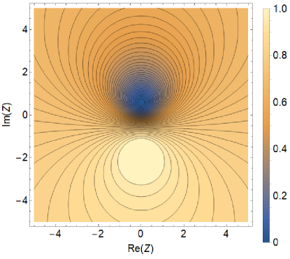
Figure 6: The contour plot of the normalized average number of quanta $\overline{N_{q}}$ on the complex $Z$ plane for $m=1$, $\Omega_{Ra}=\Omega_{Rb}$ and $\Delta\omega_{a}=\Delta\omega_{b}=\Omega$.

The contour plot of the average steady-state number of quanta normalized by its initial value,

$$\overline{N_{q}}=\displaystyle\frac{|A|^{2}\left(1+\frac{|R_{a0}|^{2}}{|R_{bm}|^{2}}\right)}{|C_{100}(0)|^{2}+|C_{010}(0)|^{2}}$$

on the complex $Z$ plane is shown in Fig. 6 for $m=1$, $\Omega_{Ra}=\Omega_{Rb}$ and $\Delta\omega_{a}=\Delta\omega_{b}=\Omega$. For this particular choice of parameters, the maximum of the number of quanta is reached at Arg$[Z]=-\pi/2$, i.e., it is located on the imaginary axis as shown in the figure. For $m=2$ the maximum will be on the real axis. At its maximum, the average number of quanta is equal to its initial value, i.e. it remains constant.

For any initial conditions other than those corresponding to the maximum of $\overline{N_{q}}$, a part of the EM field energy will dissipate through interaction with an atom, and eventually only the part which corresponds to the combination of modes completely decoupled from an atom due to destructive interference survives. This will result in smaller values of $\overline{N_{q}}$. Of course, eventually the finite cavity losses will kick in and the field will dissipate to the level of quantum and thermal fluctuations.

Finally, for the initial state $\Psi\left(0\right)=\left|0_{a}\right\rangle\left|0_{b}\right\rangle\left|1\right\rangle$ (only the atom is excited) we have $A=0$, i.e. the system goes into the ground state as expected.

To summarize, the modulated system of an atom resonantly coupled to two EM cavity modes demonstrates an interesting effect of modulation-induced transparency. In the absence of modulation, the presence of an atom experiencing an incoherent decay leads to the dissipation of the EM field even if the empty cavity is ideal, i.e. has zero losses. However, low-frequency modulation of the cavity or of the transition frequency of an atom creates the EM field distribution which is completely decoupled from an atom due to destructive interference between the cavity modes, even at resonance between the atomic transition and the cavity mode frequencies. Therefore, the atom will remain in the ground state and the field will experience no dissipation in the absence of cavity losses. For a classical field, such a destructive interference effect which switches off the field dissipation in resonant medium by introducing low-frequency modulation was considered, in particular, in Ref. rad2006 for acoustically modulated two-level atoms. Similar effects in the interaction of classical fields with atoms are discussed in the introduction of Ref. rad2020 .

V.3 Prospects for strong coupling and quantum entanglement in various nanophotonic systems

Expressions in this section and more general expressions for the relaxation rates in Appendix B (see, e.g., Eqs. (136),(137)) allow one to calculate the effective decoherence rates from the known “partial” relaxation rates for individual subsystems: EM cavity modes and any kind of a fermionic qubit. One can compare the decoherence rates with characteristic Rabi frequencies which enter the solution for the evolution equations such as Eqs. (67)-(69) in order to determine if the strong coupling regime and quantum entanglement in the electron-photon system can be achieved. For any specific application, one should also compare the effective relaxation times with relevant operation times (gate transition time, read/write time etc.) In the discussion below, we rely on the parameters obtained from Refs. haroche -aspelmeyer2014 which we already cited in the Introduction. Many of them are recent reviews and one can find further references there. We don’t attempt to overview here the vast and rapidly growing amount of literature on the subject.

In electron-based quantum emitters the largest oscillator strengths in the visible/near-infrared range have been observed for excitons in organic molecules, followed by perovskites and more conventional inorganic semiconductor quantum dots. The typical variation of the dipole matrix element of the optical transition which enters the Rabi frequency is from tens of nm to a few Angstrom. The dipole moment grows with increasing wavelength. The relaxation times are strongly temperature and material quality-dependent, varying from tens or hundreds of ps for single quantum dots at 4 K to the $\mu$s range for defects in semiconductors and diamond at mK temperatures. At room temperature the typical decoherence rates for the optical transition are in the $\sim 10$ meV range.

The photon decay times are longest for dielectric micro- and nano-cavities: photonic crystal cavities, nanopillars, distributed Bragg reflector mirrors, microdisk whispering gallery mode cavities, etc. Their quality factors are typically between $10^{3}-10^{7}$, corresponding to photon lifetimes from sub-ns to $\mu$s range. However, the field localization in the dielectric cavities is diffraction-limited, which limits the attainable Rabi frequency values to hundreds of $\mu$eV. The effective decoherence rate in dielectric cavity QED systems is typically limited by the relaxation in the fermion quantum emitter subsystem,

In plasmonic cavities, field localization on a nm and even sub-nm scale has been achieved, but the photon losses are in the ps or even fs range and therefore, they dominate the overall decoherence rate. Still, when it comes to strong coupling at room temperature to a single quantum emitter such as a single molecule or a quantum dot, the approach utilizing plasmonic cavities has seen more success so far. In these systems the Rabi splitting of the order of 100-200 meV has been observed. In plasmonic systems it may be beneficial to consider longer-wavelength emitters with the optical transition at the mid-infrared and even terahertz wavelengths. Indeed, with increasing wavelength the plasmon losses go down, the matrix element of a dipole-allowed transition increases, whereas the plasmon localization stays largely the same.

Another factor that has to be taken into account when choosing a nanophotonic system for a specific application is the rate with which the modulation of the cavity or emitter parameters has to be performed. For example, if the modulation at the rate comparable to the Rabi frequency or operation with $\pi$- or $\pi/2$ pulses is required, the plasmonic-based systems run into a problem: they would require $\sim 10-100$ fs pulses for modulation, which obviously can be achieved only with fs lasers. All electronic operations typically have a cutoff at tens of GHz. Applications of nanophotonics to quantum computing are especially challenging, because computations require at least 99.99% fidelity, i.e. at least $10^{4}$ “flops” before decoherence kicks in.

VI Conclusions

In conclusion, we developed the analytic theory describing the dynamics and control of strongly coupled nanophotonic systems with time-variable parameters. The coupling of the fermion and photon subsystems to their dissipative reservoirs are included within the stochastic equation of evolution approach, which is equivalent to the Lindblad approximation in the master equation formalism. Our analytic solution is valid in the approximation that the rate of parameter modulation and the amplitude of the frequency modulation are much smaller than the optical transition frequencies. At the same time, they can be arbitrary with respect to the generalized Rabi oscillations frequency which determines the coherent dynamics. Therefore, we can describe an arbitrary modulation of the parameters, both slower and faster than the Rabi frequency, for complete control of the quantum state. For example, one can turn on and off the entanglement between the fermionic and photonic degrees of freedom, swap between the quantum states, or decouple the fermionic qubit from the cavity field via modulation-induced transparency.

Appendix A Quantization of a cavity surface plasmon field

Consider a planar cavity oriented parallel to $(x,y)$ plane and sandwiched between two layers of material with isotropic dielectric constant $\varepsilon\left(\omega\right)$ which could be dielectric or metal. The transverse size of a cavity along $z$ is from $z=-d$ to $z=+d$. The dielectric constant inside the cavity is $\varepsilon_{g}\left(\omega\right)$, also assumed isotropic.

A.1 Spatial structure of the field and frequency dispersion

Whether or not the field is quantized, its distribution in space and frequencies of modes are determined from solving the boundary value problem of classical electrodynamics. Here we consider the field localized to a subwavelength region, to scales $l_{SP}\ll\frac{c}{\varepsilon_{g}\left(\omega\right)\omega},\frac{c}{\left|\varepsilon\left(\omega\right)\right|\omega}$ , which allows us to use electrostatic approximation. We seek the solution for the electric potential as $\varphi=\Phi\left(z\right)e^{i\mathbf{k}\cdot\mathbf{r-}i\omega t}$ , where the 2D vectors $\mathbf{r,k}$ are in the $x,y$ plane. The Poisson’s equation for the potential in every region has a form

$$\frac{\partial^{2}\Phi}{\partial z^{2}}=k^{2}\Phi$$ (91)

In the region $z<-d$ the solution is $\Phi=\Phi_{-}e^{kz}$ , whereas in $z>d$ the solution is $\Phi=\Phi_{+}e^{-kz}$.

Since the cavity is symmetric with respect to $z=0$, the spatial distribution inside the cavity can be either symmetric, $\Phi=\Phi_{s}\cosh\left(kz\right)$, or antisymmetric, $\Phi=\Phi_{as}\sinh\left(kz\right)$.

The boundary conditions include the continuity of the potential and the $z$-component of the electric induction.

(i) Symmetric solution: $\Phi_{-}=\Phi_{+}$. Substituting $z=-d$ the boundary conditions give

$$\tanh\left(kd\right)=-\frac{\varepsilon}{\varepsilon_{g}}.$$ (92)

i.e. we always need $\varepsilon\left(\omega\right)<0$ for positive $\varepsilon_{g}$. In the limit $kd\gg 1$ , Eq. (92) corresponds to the dispersion equation for a surface plasmon at the boundary between the two infinite media

$$1=-\frac{\varepsilon}{\varepsilon_{g}},$$ (93)

whereas in the opposite limit $kd\longrightarrow 0$ and assuming that $\varepsilon_{g}$ is positive and not too small, we obtain a standard dispersion equation for a plasmon in the bulk medium: $\varepsilon\left(\omega\right)=0$.

Therefore, when $kd$ changes from $0$ to $\infty$ the symmetric surface plasmon exists within a frequency bandwidth determined by the variation of $\frac{\varepsilon}{\varepsilon_{g}}$ from $-0$ to $-1$.

(ii) Antisymmetric solution: $\Phi_{-}=-\Phi_{+}$. The boundary conditions give

$$\coth\left(kd\right)=-\frac{\varepsilon}{\varepsilon_{g}}.$$ (94)

i.e. again $\varepsilon\left(\omega\right)<0$ for positive $\varepsilon_{g}$ .

In the limit of a wide cavity, when $kd\gg 1$ the solution should again corresponds to the surface plasmon at the boundary between the two infinite media, i.e. we arrive at Eq. (93).

In the opposite limit $kd\longrightarrow 0$ and assuming that $\varepsilon_{g}$ is positive and not too small, we obtain that $\varepsilon\left(\omega\right)\longrightarrow-\infty$. Therefore, when $kd$ changes from $0$ to $\infty$ the antisymmetric surface plasmon exists within a frequency bandwidth determined by the variation of $\frac{\varepsilon\left(\omega\right)}{\varepsilon_{g}\left(\omega\right)}$ from $-\infty$ to $-1$.

Note that in any case the electrostatic solution requires that $k\gg\frac{\varepsilon_{g}\omega}{c},\frac{\left|\varepsilon\right|\omega}{c}$.

A.2 Field quantization

Following Tokman2016 , we consider a cylinder with an axis of symmetry along $z$ (i.e. orthogonal to the boundaries) and area $S$ in the $x,y$ plane. We assume that the field goes to $0$ when $z\longrightarrow\pm\infty$ and satisfies periodic boundary conditions at the side surface of the cylinder:

$$\mathbf{\hat{E}}=\sum_{\mathbf{k,}p}\mathbf{E}_{\mathbf{k,}p}\left(z\right)e^{i\mathbf{k}\cdot\mathbf{r-}i\omega_{{}_{\mathbf{k,}p}}t}\hat{c}_{\mathbf{k,}p}+H_{.}c_{.},$$ (95)

where $p=s,as$ .

The spatial distribution of the field $\mathbf{E}_{\mathbf{k,}p}\left(z\right)e^{i\mathbf{k}\cdot\mathbf{r}}$ and its frequency $\omega_{{}_{\mathbf{k,}p}}$ are given by the solution of the classical boundary value problem in the previous section. The Hamiltonian $\hat{H}=\hbar\sum_{\mathbf{k,}p}\omega_{\mathbf{k,}p}\left(\hat{c}_{\mathbf{k,}p}^{\dagger}\hat{c}_{\mathbf{k,}p}+\frac{1}{2}\right)$ can be obtained from the normalization condition Tokman2016 :

$$S\int_{-\infty}^{\infty}\left(\frac{\partial\left[\omega\varepsilon\left(\omega,z\right)\right]}{\partial\omega}\mathbf{E}_{\mathbf{k,}p}^{\ast}\left(z\right)\mathbf{E}_{\mathbf{k,}p}\left(z\right)+\mathbf{B}_{\mathbf{k,}p}^{\ast}\left(z\right)\mathbf{B}_{\mathbf{k,}p}\left(z\right)\right)dz=4\pi\hbar\omega_{{}_{\mathbf{k,}p}}$$ (96)

where $S\int_{-\infty}^{\infty}\left(\cdot\cdot\cdot\right)dz=$ $\int_{V}\left(\cdot\cdot\cdot\right)dV$. For periodic or “cavity” boundary conditions we always have Tokman2016 :

$$\int_{V}\mathbf{B}_{\mathbf{k,}p}^{\ast}\mathbf{B}_{\mathbf{k,}p}dV=\int_{V}\varepsilon\mathbf{E}_{\mathbf{k,}p}^{\ast}\mathbf{E}_{\mathbf{k,}p}dV,$$ (97)

Which allows us to rewrite Eq. (96) as

$$S\int_{-\infty}^{\infty}\frac{\partial\left[\omega^{2}\varepsilon\left(\omega,z\right)\right]}{\omega\partial\omega}\mathbf{E}_{\mathbf{k,}p}^{\ast}\left(z\right)\mathbf{E}_{\mathbf{k,}p}\left(z\right)dz=4\pi\hbar\omega_{{}_{\mathbf{k,}p}}.$$ (98)

For the fields $\mathbf{E}_{\mathbf{k,}p}\left(z\right)$ obtained in the electrostatic approximation, we always obtain $\int_{V}\varepsilon\mathbf{E}_{\mathbf{k,}p}^{\ast}\mathbf{E}_{\mathbf{k,}p}dV=0$ , since in this approximation $\mathbf{B}_{\mathbf{k,}p}=0$. In this case we can use the normalization in the electrostatic limit:

$$S\int_{-\infty}^{\infty}\frac{\partial\left[\omega\varepsilon\left(\omega,z\right)\right]}{\partial\omega}\mathbf{E}_{\mathbf{k,}p}^{\ast}\left(z\right)\mathbf{E}_{\mathbf{k,}p}\left(z\right)dz=4\pi\hbar\omega_{{}_{\mathbf{k,}p}}.$$ (99)

As a result, we obtain:

(i) Symmetric mode ($p=s$). The normalization condition:

$$S\left|\Phi_{s}\right|^{2}k\left[\frac{\partial\left(\omega\varepsilon_{g}\right)}{\partial\omega}\sinh\left(2kd\right)+2\cosh^{2}\left(kd\right)\frac{\partial\left(\omega\varepsilon\right)}{\partial\omega}\right]=4\pi\hbar\omega_{{}_{\mathbf{k,}s}}$$ (100)

(ii)Antisymmetric mode ($p=as$). The normalization condition:

$$S\left|\Phi_{as}\right|^{2}k\left[\frac{\partial\left(\omega\varepsilon_{g}\right)}{\partial\omega}\sinh\left(2kd\right)+2\sinh^{2}\left(kd\right)\frac{\partial\left(\omega\varepsilon\right)}{\partial\omega}\right]=4\pi\hbar\omega_{{}_{\mathbf{k,}as}}$$ (101)

Taking for simplicity $\varepsilon_{g}=1$ (air) and $\varepsilon\left(\omega\right)=1-\frac{\omega_{pl}^{2}}{\omega^{2}}$ (Drude dispersion) gives

(i) Symmetric mode ($p=s$):

$$S\left|\Phi_{s}\right|^{2}k\left[2\sinh\left(2kd\right)+4\cosh^{2}\left(kd\right)\right]=4\pi\hbar\omega_{{}_{\mathbf{k,}s}}$$ (102)

(ii)Antisymmetric mode ($p=as$):

$$S\left|\Phi_{as}\right|^{2}k\left[2\sinh\left(2kd\right)+4\sinh^{2}\left(kd\right)\right]=4\pi\hbar\omega_{{}_{\mathbf{k,}as}}$$ (103)

In order to calculate the coupling strength, it is important to know the magnitude of the normalization field $\mathbf{E}_{\mathbf{k,}p}$ at the cavity boundary. Introducing the notation $\mathbf{E}_{\mathbf{k,}p}\left(-d\right)=\mathbf{\tilde{E}}_{\mathbf{k,}p}$ and taking into account Eqs. (A.1),(A.1),(102) and (103), we obtain

$$\mathbf{\tilde{E}}_{\mathbf{k,}s}=\left[\mathbf{z}_{0}k\sinh\left(kd\right)-i\mathbf{k}\cosh\left(kd\right)\right]\sqrt{\frac{4\pi\hbar\omega_{{}_{\mathbf{k,}s}}}{Sk\left[2\sinh\left(2kd\right)+4\cosh^{2}\left(kd\right)\right]}},$$ (104)

where

$$\omega_{{}_{\mathbf{k,}s}}=\frac{\omega_{pl}}{\sqrt{1+\tanh\left(kd\right)}};$$ (105)

$$\mathbf{\tilde{E}}_{\mathbf{k,}as}=\left[-\mathbf{z}_{0}k\cosh\left(kd\right)-i\mathbf{k}\sinh\left(kd\right)\right]\sqrt{\frac{4\pi\hbar\omega_{{}_{\mathbf{k,}as}}}{Sk\left[2\sinh\left(2kd\right)+4\cosh^{2}\left(kd\right)\right]}},$$ (106)

where

$$\omega_{{}_{\mathbf{k,}as}}=\frac{\omega_{pl}}{\sqrt{1+\coth\left(kd\right)}}.$$ (107)

Figure 7 shows an example of normalized frequencies and field amplitudes of the symmetric and antisymmetric cavity modes given by Eqs. (104)-(107) as a function of normalized time $\Omega t$ when the cavity height $d$ is modulated as $d(t)=d_{0}(1+0.1\sin(\Omega t))$. In this example $kd_{0}=1$. Even though the dependence of frequencies and field amplitudes on $kd$ is strongly nonlinear, their modulation amplitudes remain small.

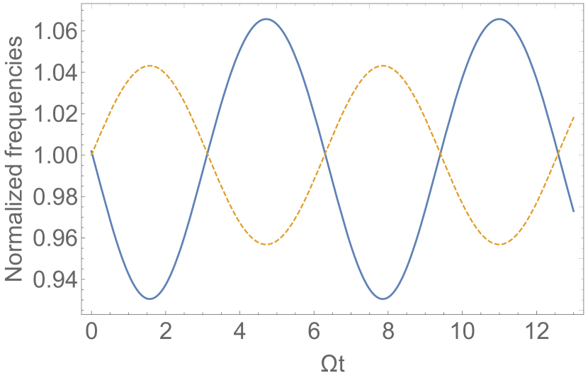
(a)

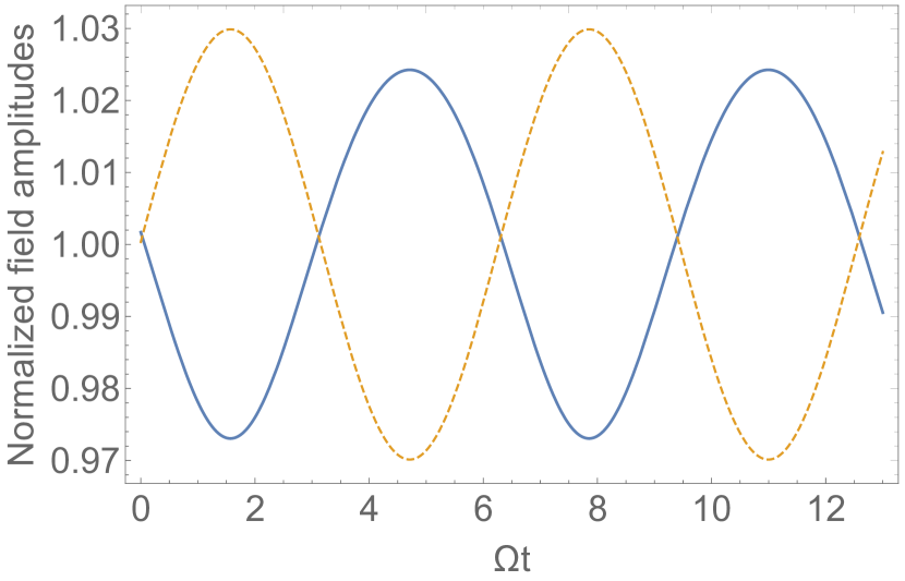
(b)

Figure 7: (a) Normalized frequencies and (b) normalized field amplitudes of the symmetric (solid line) and antisymmetric (dashed line) cavity modes given by Eqs. (104)-(107) as a function of normalized time $\Omega t$ when the cavity height $d$ is modulated as $d(t)=d_{0}(1+0.1\sin(\Omega t))$, where $kd_{0}=1$. Frequencies and field amplitudes are normalized by their time-averaged values.

A.3 Field quantization when the cavity thickness is changing adiabatically

Let the cavity half-thickness $d$ change with time adiabatically, $d\left(t\right)$, for given $k$ and $S$. In this case the adiabatic invariant $\frac{W_{\mathbf{k,}p}}{\omega_{{}_{\mathbf{k,}p}}}$ is conserved, where $W_{\mathbf{k,}p}$ is an average (observable) energy of the mode. This is equivalent to conservation of the number of photons in a cavity with slowly changing parameters. As is well known, the photon number is conserved for a standard Hamiltonian of an ensemble of harmonic oscillators:

$$\hat{H}=\hbar\sum_{\mathbf{k,}p}\omega_{\mathbf{k,}p}\left(\hat{c}_{\mathbf{k,}p}^{\dagger}\hat{c}_{\mathbf{k,}p}+\frac{1}{2}\right),$$ (108)

whereas the normalization field is still described by Eqs. (100),(101). At the same time, all results will contain the variables $\omega_{{}_{\mathbf{k,}p}}\left(t\right)$ and $\mathbf{\tilde{E}}_{\mathbf{k,}p}$ $\left(t\right)$ which depend on time through their dependence on the parameter $d(t)$.

Appendix B The stochastic equation of evolution for the state vector

The description of open quantum systems within the stochastic equation of evolution for the state vector is usually formulated for a Monte-Carlo type numerical scheme, e.g. the method of quantum jumps Scully1997 ; Plenio1998 . We developed an approach suitable for analytic derivations. Our stochastic equation of evolution is basically the Schrödinger equation modified by adding a linear relaxation operator and the noise source term with appropriate correlation properties. The latter are related to the parameters of the relaxation operator in such a way that the expressions for the statistically averaged quantities satisfy certain physically meaningful conditions.

The protocol of introducing the relaxation operator with a corresponding noise source term to the quantum dynamics is well known in the Heisenberg picture, where it is called the Heisenberg-Langevin method Scully1997 ; Gardiner2004 ; Tokman2013 . Here we use a conceptually similar approach for the Schrödinger equation. The general form of the stochastic equation of evolution was derived from the Heisenberg-Langevin equations in tokman2020 . Here we outline how certain physically reasonable constraints on the observables determine the correlation properties of the noise sources.

B.1 General properties of the stochastic equation of evolution for the state vector

An open system interacting with a reservoir is generally in a mixed state and should be described by the density matrix. We are describing the state of the system with a state vector which has a fluctuating component. For example, in a certain basis $\left|\alpha\right\rangle$ the state vector will be $C_{\alpha}\left(t\right)=\overline{C_{\alpha}}+\widetilde{C_{\alpha}}$, where the fluctuating component is denoted with a wavy bar. The elements of the density matrix of the corresponding mixed state are $\rho_{\alpha\beta}=\overline{C_{\alpha}C_{\beta}^{\ast}}=\overline{C_{\alpha}}\cdot\overline{C_{\beta}^{\ast}}+\overline{\widetilde{C_{\alpha}}\cdot\widetilde{C_{\beta}}^{\ast}}$.

The stochastic equation of evolution for the state vector and its Hermitian conjugate have the general form tokman2020

$$\frac{d}{dt}\left|\Psi\right\rangle=-\frac{i}{\hbar}\hat{H}_{eff}\left|\Psi\right\rangle-\frac{i}{\hbar}\left|\mathfrak{R}\left(t\right)\right\rangle$$ (109)

$$\frac{d}{dt}\left\langle\Psi\right|=\frac{i}{\hbar}\left\langle\Psi\right|\hat{H}_{eff}^{\dagger}+\frac{i}{\hbar}\left\langle\mathfrak{R}\left(t\right)\right|,$$ (110)

where the non-Hermitian component of the effective Hamiltonian $\hat{H}_{eff}$ corresponds to the relaxation operator and the term $\left|\mathfrak{R}\left(t\right)\right\rangle$ denotes the noise term. We will also need Eqs. (109) and (110) in a particular basis $\left|\alpha\right\rangle$:

$$\frac{d}{dt}C_{\alpha}=-\frac{i}{\hbar}\sum_{\nu}\left(\hat{H}_{eff}\right)_{\alpha\nu}C_{\nu}-\frac{i}{\hbar}\mathfrak{R}_{\alpha},$$ (111)

$$\frac{d}{dt}C_{\alpha}^{\ast}=\frac{i}{\hbar}\sum_{\nu}C_{\nu}^{\ast}\left(\hat{H}_{eff}^{\dagger}\right)_{\nu\alpha}+\frac{i}{\hbar}\mathfrak{R}_{\alpha}^{\ast},$$ (112)

where $\mathfrak{R}_{\alpha}=\left\langle\alpha\right.\left|\mathfrak{R}\right\rangle$, $\left(\hat{H}_{eff}\right)_{\alpha\beta}=\left\langle\alpha\right|\hat{H}_{eff}\left|\beta\right\rangle$.

In general, statistical properties of noise that ensure certain physically meaningful requirements impose certain constraints on the noise source $\left|\mathfrak{R}\right\rangle$ which enters the right-hand side of the stochastic equation for the state vector. In particular, it is natural to require that the statistically averaged quantity $\overline{\left|\mathfrak{R}\right\rangle}=0$. We will also require that the noise source $\left|\mathfrak{R}\right\rangle$ has the correlation properties that preserve the norm of the state vector averaged over the reservoir statistics:

$$\overline{\left\langle\Psi\left(t\right)\right.\left|\Psi\left(t\right)\right\rangle}=1.$$ (113)

B.2 Noise correlator

The solution to Eqs. (109) and (110) can be formally written as

$$\left|\Psi\right\rangle=e^{-\frac{i}{\hbar}\hat{H}_{eff}t}\left|\Psi_{0}\right\rangle-\frac{i}{\hbar}\int_{0}^{t}e^{\frac{i}{\hbar}\hat{H}_{eff}\left(\tau-t\right)}\left|\mathfrak{R}\left(\tau\right)\right\rangle d\tau,$$ (114)

$$\left\langle\Psi\right|=\left\langle\Psi_{0}\right|e^{\frac{i}{\hbar}\hat{H}_{eff}^{\dagger}t}+\frac{i}{\hbar}\int_{0}^{t}\left\langle\mathfrak{R}\left(\tau\right)\right|e^{-\frac{i}{\hbar}\hat{H}_{eff}^{\dagger}\left(\tau-t\right)}d\tau,$$ (115)

In the basis $|\alpha\rangle$, Eqs. (114),(115) can be transformed into

$$C_{\alpha}=\left\langle\alpha\right|e^{-\frac{i}{\hbar}\hat{H}_{eff}t}\left|\Psi_{0}\right\rangle-\frac{i}{\hbar}\int_{0}^{t}\left\langle\alpha\right|e^{\frac{i}{\hbar}\hat{H}_{eff}\left(\tau-t\right)}\left|\mathfrak{R}\left(\tau\right)\right\rangle d\tau,$$ (116)

$$C_{\alpha}^{\ast}=\left\langle\Psi_{0}\right|e^{\frac{i}{\hbar}\hat{H}_{eff}^{\dagger}t}\left|\alpha\right\rangle+\frac{i}{\hbar}\int_{0}^{t}\left\langle\mathfrak{R}\left(\tau\right)\right|e^{-\frac{i}{\hbar}\hat{H}_{eff}^{\dagger}\left(\tau-t\right)}\left|\alpha\right\rangle d\tau.$$ (117)

In order to calculate the observables, we need to know the expressions for the averaged dyadic combinations of the amplitudes. We can find them using Eqs. (111) and (112):

$$\frac{d}{dt}\overline{C_{\alpha}C_{\beta}^{\ast}} = -\frac{i}{\hbar}\sum_{\nu}\left(H_{\alpha\nu}^{\left(h\right)}\overline{C_{\nu}C_{\beta}^{\ast}}-\overline{C_{\alpha}C_{\nu}^{\ast}}H_{\nu\beta}^{\left(h\right)}\right)-\frac{i}{\hbar}\sum_{\nu}\left(H_{\alpha\nu}^{\left(ah\right)}\overline{C_{\nu}C_{\beta}^{\ast}}+\overline{C_{\alpha}C_{\nu}^{\ast}}H_{\nu\beta}^{\left(ah\right)}\right)$$ (118)

$$+\left(-\frac{i}{\hbar}\overline{C_{\beta}^{\ast}\mathfrak{R}_{\alpha}}+\frac{i}{\hbar}\overline{\mathfrak{R}_{\beta}^{\ast}C_{\alpha}}\right),$$

where we separated the Hermitian and anti-Hermitian components of the effective Hamiltonian: $\left\langle\alpha\right|\hat{H}_{eff}\left|\beta\right\rangle=H_{\alpha\beta}^{\left(h\right)}+H_{\alpha\beta}^{\left(ah\right)}$. Substituting Eqs. (116) and (117) into the last term in Eq. (118), we obtain

$$-\frac{i}{\hbar}\overline{C_{\beta}^{\ast}\mathfrak{R}_{\alpha}}+\frac{i}{\hbar}\overline{C_{\alpha}\mathfrak{R}_{\beta}^{\ast}} = \frac{1}{\hbar^{2}}\int_{-t}^{0}\overline{\left\langle\mathfrak{R}\left(t+\xi\right)\right|e^{-\frac{i}{\hbar}\hat{H}_{eff}^{\dagger}\xi}\left|\beta\right\rangle\left\langle\alpha\right.\left|\mathfrak{R}\left(t\right)\right\rangle}d\xi$$

$$+\frac{1}{\hbar^{2}}\int_{-t}^{0}\overline{\left\langle\mathfrak{R}\left(t\right)\right.\left|\beta\right\rangle\left\langle\alpha\right|e^{\frac{i}{\hbar}\hat{H}_{eff}\xi}\left|\mathfrak{R}\left(t+\xi\right)\right\rangle}d\xi.$$

To proceed further with analytical results, we need to evaluate these integrals. The simplest situation is when the noise source terms are delta-correlated in time (Markovian). In this case only the point $\xi=0$ contributes to the integrals. As a result, Eq. (118)) is transformed to

$$\frac{d}{dt}\overline{C_{\alpha}C_{\beta}^{\ast}}=-\frac{i}{\hbar}\sum_{\nu}\left(H_{\alpha\nu}^{\left(h\right)}\overline{C_{\nu}C_{\beta}^{\ast}}-\overline{C_{\alpha}C_{\nu}^{\ast}}H_{\nu\beta}^{\left(h\right)}\right)-\frac{i}{\hbar}\sum_{\nu}\left(H_{\alpha\nu}^{\left(ah\right)}\overline{C_{\nu}C_{\beta}^{\ast}}+\overline{C_{\alpha}C_{\nu}^{\ast}}H_{\nu\beta}^{\left(ah\right)}\right)+D_{\alpha\beta},$$ (119)

where the correlator $D_{\alpha\beta}$ is defined by

$$\overline{\mathfrak{R}_{\beta}^{\ast}\left(t+\xi\right)\mathfrak{R}_{\alpha}\left(t\right)}=\overline{\mathfrak{R}_{\beta}^{\ast}\left(t\right)\mathfrak{R}_{\alpha}\left(t+\xi\right)}=\hbar^{2}\delta\left(\xi\right)D_{\alpha\beta}.$$ (120)

The time derivative of the norm of the state vector is given by

$$\frac{d}{dt}\sum_{\alpha}\overline{\left|C_{\alpha}\right|^{2}}=-\sum_{\alpha}\left[\frac{i}{\hbar}\sum_{\nu}\left(H_{\alpha\nu}^{\left(ah\right)}\overline{C_{\nu}C_{\alpha}^{\ast}}+\overline{C_{\alpha}C_{\nu}^{\ast}}H_{\nu\alpha}^{\left(ah\right)}\right)-D_{\alpha\alpha}\right].$$ (121)

Clearly, the components $D_{\alpha\alpha}$ of the noise correlator need to compensate the decrease in the norm due to the anti-Hermitian component of the effective Hamiltonian. Therefore the expressions for $H_{\alpha\beta}^{\left(ah\right)}$and $D_{\alpha\alpha}$ have to be mutually consistent. This is the manifestation of the fluctuation-dissipation theorem Landau1965 .

As an example, consider a simple diagonal anti-Hermitian operator $H_{\alpha\nu}^{\left(ah\right)}$:

$$H_{\alpha\nu}^{\left(ah\right)}=-i\hbar\gamma_{\alpha}\delta_{\alpha\nu}$$ (122)

and introduce the following models:

(i) Populations relax much slower than coherences (expected for condensed matter systems). In this case we can choose $D_{\alpha\neq\beta}=0$, $D_{\alpha\alpha}=2\gamma_{\alpha}\overline{\left|C_{\alpha}\right|^{2}}$; within this model the population at each state will be preserved.

(ii) The state $\alpha=\alpha_{down}$ has a minimal energy, while the reservoir temperature $T=0$. In this case it is expected that all populations approach zero in equilibrium whereas the occupation number of the ground state approaches $1$, similar to the Weisskopf-Wigner model. The adequate choice of correlators is $D_{\alpha\neq\beta}=0$, $D_{\alpha\alpha}\propto\delta_{\alpha\alpha_{down}}$, $\gamma_{\alpha_{down}}=0$. The expression for the remaining nonzero correlator,

$$D_{\alpha_{down}\alpha_{down}}=\sum_{\alpha\neq\alpha_{down}}2\gamma_{\alpha}\overline{\left|C_{\alpha}\right|^{2}},$$ (123)

ensures the conservation of the norm:

$$\frac{d}{dt}\sum_{\alpha\neq\alpha_{down}}\overline{\left|C_{\alpha}\right|^{2}}=-\sum_{\alpha\neq\alpha_{down}}2\gamma_{\alpha}\overline{\left|C_{\alpha}\right|^{2}}=-\frac{d}{dt}\overline{\left|C_{\alpha_{down}}\right|^{2}}.$$

This is an example of the correlator’s dependence on the state vector that we discussed before.

(iii) A two-level system with states $|0\rangle$ and $|1\rangle$ and relaxation rates of populations $\frac{1}{T_{1}}$ and coherence $\frac{1}{T_{2}}=\frac{1}{2T_{1}}+\gamma_{el}$, where $\gamma_{el}$ is an elastic relaxation constant. If the equilibrium corresponds to a zero population of the excited state, we have to choose

$$\gamma_{0}=0,\;\gamma_{1}=\frac{1}{T_{2}},\;D_{10}=D_{01}=0,\;D_{00}=\frac{1}{T_{1}}\overline{|C_{1}|^{2}},\;D_{11}=2\gamma_{el}\overline{|C_{1}|^{2}}.$$

It is easy to see that with this choice of relaxation constants and noise correlators Eqs. (119) for $\overline{C_{\alpha}C_{\beta}^{\ast}}$ where $\alpha,\beta=1,2$ coincide with well-known equations for the density matrix $\rho_{\alpha\beta}$ of a two-level system Scully1997 ; fain .

B.3 Comparison with the Lindblad method

One can choose the anti-Hermitian Hamiltonian $H_{\alpha\beta}^{\left(ah\right)}$ and correlators $D_{\alpha\beta}$ in the stochastic equation of motion in such a way that Eq. (119) for the dyadics $\overline{C_{n}C_{m}^{\ast}}$ correspond exactly to the equations for the density matrix elements in the Lindblad approach. Indeed, the Lindblad form of the master equation has the form Scully1997 ; Plenio1998

$$\frac{d}{dt}\hat{\rho}=-\frac{i}{\hbar}\left[\hat{H},\hat{\rho}\right]+\hat{L}\left(\hat{\rho}\right)$$ (124)

where $\hat{L}\left(\hat{\rho}\right)$ is the Lindbladian:

$$\hat{L}\left(\hat{\rho}\right)=-\frac{1}{2}\sum_{k}\gamma_{k}\left(\hat{l}_{k}^{\dagger}\hat{l}_{k}\hat{\rho}+\hat{\rho}\hat{l}_{k}^{\dagger}\hat{l}_{k}-2\hat{l}_{k}\hat{\rho}\hat{l}_{k}^{\dagger}\right),$$ (125)

Operators $\hat{l}_{k}$ in Eq. (125) and their number are determined by the model which describes the coupling of the dynamical system to the reservoir. The form of the relaxation operator given by Eq. (125) preserves automatically the conservation of the trace of the density matrix, whereas the specific choice of relaxation constants ensures that the system approaches a proper steady state given by thermal equilibrium or supported by an incoherent pumping.

Eq. (124) is convenient to represent in a slightly different form:

$$\frac{d}{dt}\hat{\rho}=-\frac{i}{\hbar}\left(\hat{H}_{eff}\hat{\rho}-\hat{\rho}\hat{H}_{eff}^{\dagger}\right)+\delta\hat{L}\left(\hat{\rho}\right)$$ (126)

where

$$\hat{H}_{eff}=\hat{H}-i\hbar\sum_{k}\gamma_{k}\hat{l}_{k}^{\dagger}\hat{l}_{k},~{}~{}~{}\delta\hat{L}\left(\hat{\rho}\right)=\sum_{k}\gamma_{k}\hat{l}_{k}\hat{\rho}\hat{l}_{k}^{\dagger}.$$ (127)

Writing the anti-Hermitian component of the Hamiltonian in Eqs. (111),(112) as

$$H_{\alpha\beta}^{\left(ah\right)}=-i\hbar\left\langle\alpha\right|\sum_{k}\gamma_{k}\hat{l}_{k}^{\dagger}\hat{l}_{k}\left|\beta\right\rangle,$$ (128)

and defining the corresponding correlator of the noise source as

$$\overline{\mathfrak{R}_{\beta}^{\ast}\left(t+\xi\right)\mathfrak{R}_{\alpha}\left(t\right)}=\hbar^{2}\delta\left(\xi\right)D_{\alpha\beta},~{}~{}~{}~{}D_{\alpha\beta}=\left\langle\alpha\right|\delta\hat{L}\left(\hat{\rho}\right)\left|\beta\right\rangle_{\rho_{nm}=\overline{C_{n}C_{m}^{\ast}}},$$ (129)

we obtain the solution in which averaged over noise statistics dyadics $\overline{C_{n}C_{m}^{\ast}}$ correspond exactly to the elements of the density matrix within the Lindblad method.

Instead of deriving the stochastic equation of evolution of the state vector from the Heisenberg-Langevin equations we could postulate it from the very beginning. After that, we could justify the choice of the effective Hamiltonian and noise correlators by ensuring that they lead to the same observables as the solution of the density matrix equations with the relaxation operator in Lindblad form Plenio1998 ; blum . However, the demonstration of direct connection between the stochastic equation of evolution of the state vector and the Heisenberg-Langevin equation provides an important physical insight.

B.4 Relaxation rates for coupled subystems interacting with a reservoir

Whenever we have several coupled subsystems (such as electrons, photon modes, phonons etc.), each coupled to its reservoir, the determination of relaxation rates of the whole system becomes nontrivial. The problem can be solved if we assume that these “partial” reservoirs are statistically independent.In this case it is possible to add up partial Lindbladians and obtain the total effective Hamiltonian.

Consider again the Hamiltonian (27) for a two-level electron system resonantly coupled to two quantized EM cavity modes,

$$\hat{H}=\hbar\omega_{a}\left(t\right)\left(\hat{a}^{\dagger}\hat{a}+\frac{1}{2}\right)+\hbar\omega_{b}\left(t\right)\left(\hat{b}^{\dagger}\hat{b}+\frac{1}{2}\right)+W\hat{\sigma}^{\dagger}\hat{\sigma}+\hat{V},$$ (130)

where

$$\hat{V}=-\hat{\sigma}^{\dagger}\left(\chi_{a}\hat{a}+\chi_{b}\hat{b}\right)-\hat{\sigma}\left(\chi_{a}^{\ast}\hat{a}^{\dagger}+\chi_{b}^{\ast}\hat{b}^{\dagger}\right)$$

and $\chi_{a,b}\left(t\right)=\mathbf{d\cdot E}_{a,b}$.

Summing up the known (see e.g. Scully1997 ; Plenio1998 ) partial Lindbladians of two bosonic (infinite amount of energy levels) and one fermionic (two-level) subsystems, we obtain

$$L\left(\hat{\rho}\right) = -\frac{\gamma}{2}N_{1}^{T_{a}}\left(\hat{\sigma}\hat{\sigma}^{\dagger}\hat{\rho}+\hat{\rho}\hat{\sigma}\hat{\sigma}^{\dagger}-2\hat{\sigma}^{\dagger}\hat{\rho}\hat{\sigma}\right)-\frac{\gamma}{2}N_{0}^{T_{a}}\left(\hat{\sigma}^{\dagger}\hat{\sigma}\hat{\rho}+\hat{\rho}\hat{\sigma}^{\dagger}\hat{\sigma}-2\hat{\sigma}\hat{\rho}\hat{\sigma}^{\dagger}\right)$$ (131)

$$-\frac{\mu_{a}}{2}\overline{n}_{a}^{T_{em}}\left(\hat{a}\hat{a}^{\dagger}\hat{\rho}+\hat{\rho}\hat{a}^{\dagger}\hat{a}-2\hat{a}^{\dagger}\hat{\rho}\hat{a}\right)-\frac{\mu_{a}}{2}\left(\overline{n}_{a}^{T_{em}}+1\right)\left(\hat{a}^{\dagger}\hat{a}\hat{\rho}+\hat{\rho}\hat{a}\hat{a}^{\dagger}-2\hat{a}\hat{\rho}\hat{a}^{\dagger}\right)$$

$$-\frac{\mu_{b}}{2}\overline{n}_{b}^{T_{em}}\left(\hat{b}\hat{b}^{\dagger}\hat{\rho}+\hat{\rho}\hat{b}^{\dagger}\hat{b}-2\hat{b}^{\dagger}\hat{\rho}\hat{b}\right)-\frac{\mu_{b}}{2}\left(\overline{n}_{b}^{T_{em}}+1\right)\left(\hat{b}^{\dagger}\hat{b}\hat{\rho}+\hat{\rho}\hat{b}\hat{b}^{\dagger}-2\hat{b}\hat{\rho}\hat{b}^{\dagger}\right),$$

where $\gamma$ is an inelastic relaxation constant for an isolated atom, $\mu_{a,b}$ are relaxation constants of the EM modes determined by the cavity Q-factor;

$$N_{0}^{T_{a}}=\frac{1}{1+e^{-\frac{W}{T_{a}}}},\;N_{1}^{T_{a}}=\frac{{}^{e^{-\frac{W}{T_{a}}}}}{1+e^{-\frac{W}{T_{a}}}},\;\overline{n}_{a,b}^{T_{em}}=\frac{1}{e^{\frac{\hbar\omega_{a,b}}{T_{em}}}-1},$$

where $T_{a,em}$ are the temperatures of the atomic and EM dissipative reservoirs, respectively. It is assumed that these reservoirs are statistically independent.

For the Lindblad master equation in the form Eq. (126) we get

$$\hat{H}_{eff}=\hat{H}-i\hat{\Lambda},$$ (132)

where

$$\hat{\Lambda}=\frac{\hbar}{2}\left\{\gamma\left(N_{1}^{T_{a}}\hat{\sigma}\hat{\sigma}^{\dagger}+N_{0}^{T_{a}}\hat{\sigma}^{\dagger}\hat{\sigma}\right)+\mu_{a}\left[\overline{n}_{a}^{T_{em}}\hat{a}\hat{a}^{\dagger}+\left(\overline{n}_{a}^{T_{em}}+1\right)\hat{a}^{\dagger}\hat{a}\right]+\mu_{b}\left[\overline{n}_{b}^{T_{em}}\hat{b}\hat{b}^{\dagger}+\left(\overline{n}_{b}^{T_{em}}+1\right)\hat{b}^{\dagger}\hat{b}\right]\right\}.$$ (133)

Using the effective Hamiltonian given by Eqs. (132),(133), we arrive at the stochastic equation for the state vector in the following form:

$$\left(\frac{\partial}{\partial t}+\gamma_{n_{a}n_{b}1}\right)C_{n_{a}n_{b}1}+i\left(\left(n_{a}+\frac{1}{2}\right)\omega_{a}\left(t\right)+\left(n_{b}+\frac{1}{2}\right)\omega_{b}\left(t\right)+\frac{W}{\hbar}\right)C_{n_{a}n_{b}1}$$

$$-\frac{i}{\hbar}\left\langle n_{a}\right|\left\langle n_{b}\right|\left\langle 1\right|\hat{V}\left|\Psi\right\rangle=-\frac{i}{\hbar}\mathfrak{R}_{n_{a}n_{b}1},$$ (134)

$$\left(\frac{\partial}{\partial t}+\gamma_{n_{a}n_{b}0}\right)C_{n_{a}n_{b}0}+i\left(\left(n_{a}+\frac{1}{2}\right)\omega_{a}\left(t\right)+\left(n_{b}+\frac{1}{2}\right)\omega_{b}\left(t\right)\right)C_{n_{a}n_{b}0}$$

$$-\frac{i}{\hbar}\left\langle n_{a}\right|\left\langle n_{b}\right|\left\langle 0\right|\hat{V}\left|\Psi\right\rangle=-\frac{i}{\hbar}\mathfrak{R}_{n_{a}n_{b}0},$$ (135)

where

$$\gamma_{n_{a}n_{b}0}=\frac{\gamma}{2}N_{1}^{T_{a}}+\frac{\mu_{a}}{2}\left[\overline{n}_{a}^{T_{em}}\left(n_{a}+1\right)+\left(\overline{n}_{a}^{T_{em}}+1\right)n_{a}\right]+\frac{\mu_{b}}{2}\left[\overline{n}_{b}^{T_{em}}\left(n_{b}+1\right)+\left(\overline{n}_{b}^{T_{em}}+1\right)n_{b}\right],$$ (136)

$$\gamma_{n_{a}n_{b}1}=\frac{\gamma}{2}N_{0}^{T_{a}}+\frac{\mu_{a}}{2}\left[\overline{n}_{a}^{T_{em}}\left(n_{a}+1\right)+\left(\overline{n}_{a}^{T_{em}}+1\right)n_{a}\right]+\frac{\mu_{b}}{2}\left[\overline{n}_{b}^{T_{em}}\left(n_{b}+1\right)+\left(\overline{n}_{b}^{T_{em}}+1\right)n_{b}\right],$$ (137)

Eqs. (136),(137) determine the rules of combining the “partial” relaxation rates for several coupled subsystems.

The above expressions include only inelastic relaxation rates. The general procedure of adding elastic relaxation (pure dephasing) is described in tokman2020 . For the simple RWA models considered in this paper this procedure is reduced to adding $\gamma_{el}$ to $\gamma_{001}$ and changing the noise correlator according to $D_{001;001}\Rightarrow D_{001;001}+2\gamma_{el}\overline{|C_{001}|^{2}}$.

References

- (1) S. Haroche and J. M. Raymond, Exploring the Quantum. Atoms, Cavities, and photons (Oxford University Press, Oxford, UK, 2006).
- (2) P. Lodahl, S. Mahmoodian, and S. Stobbe, Interfacing single photons and single quantum dots with photonic nanostructures, Rev. Mod. Phys. 87, 347 (2015).
- (3) C. L. Degen, F. Reinhard, and P. Cappellaro, Quantum sensing, Rev. Mod. Phys. 89, 035002 (2017).
- (4) A. Sipahigil, R. E. Evans, D. D. Sukachev, et al., An integrated diamond nanophotonics platform for quantum-optical networks, Science 354, 847 (2016).
- (5) T. Yoshie, A. Scherer, J. Hendrickson, G. Khitrova, H. M. Gibbs, G. Rupper, C. Ell, O. B. Shchekin, and D. G. Deppe, Vacuum Rabi splitting with a single quantum dot in a photonic crystal nanocavity, Nature 432, 200 (2004).
- (6) J. P. Reithmaier, G. Sek, A. Loffler, C. Hofmann, S. Kuhn, S. Reitzenstein, L. V. Keldysh, V. D. Kulakovskii, T. L. Reinecke, and A. Forchel, Strong coupling in a single quantum dot–semiconductor microcavity system, Nature 432, 197 (2004).
- (7) R. Chikkaraddy, B. de Nijs, F. Benz, S. J. Barrow, O. A. Scherman, E. Rosta, A. Demetriadou, P. Fox, O. Hess, and J. J. Baumberg, Single-molecule strong coupling at room temperature in plasmonic nanocavities, Nature 535, 127 (2016).
- (8) F. Benz, M. K. Schmidt, A. Dreismann, R. Chikkaraddy, Y. Zhang, A. Demetriadou, C. Carnegie, H. Ohadi, B. de Nijs, R. Esteban, J. Aizpurua, and J. J. Baumberg, Single-molecule optomechanics in picocavities, Science 354, 726 (2016).
- (9) K.-D. Park, E. A. Muller, V. Kravtsov, P. M. Sass, J. Dreyer, J. M. Atkin, and M. B. Raschke, Variable-temperature tip-enhanced Raman spectroscopy of single-molecule fluctuations and dynamics, Nano Lett. 16, 479 (2016).
- (10) H. Leng, B. Szychowski, M.-C. Daniel, and M. Pelton, Strong coupling and induced transparency at room temperature with single quantum dots and gap plasmons, Nat Commun. 9, 4012 (2018).
- (11) H. Gross, J. M. Hamm, T. Tufarelli, O. Hess, and B. Hecht, Near-field strong coupling of single quantum dots, Sci. Adv. 2018; 4: eaar4906.
- (12) K.-D. Park, M. A. May, H. Leng, J. Wang, J. A. Kropp, T. Gougousi, M. Pelton, M. B. Raschke, Tip-enhanced strong coupling spectroscopy, imaging, and control of a single quantum emitter, Sci. Adv. 2019;5: eaav5931.
- (13) P. Törma and W. L. Barnes, Strong coupling between surface plasmon polaritons and emitters: a review, Rep. Prog. Phys. 78, 013901 (2015).
- (14) O. Bitton, S. N. Gupta, and G. Haran, Quantum dot plasmonics: from weak to strong coupling, Nanophotonics 8, 559 (2019).
- (15) P. Forn-Diaz, L. Lamata, E. Rico, J. Kono, and E. Solano, Ultrastrong coupling regimes of light-matter interaction, Rev. Mod. Phys. 91, 025005 (2019).
- (16) M. A. May, D. Fialkow, T. Wu, K.-D. Park, H. Leng, J. A. Kropp, T. Gougousi, P. Lalanne, M. Pelton, and M. B. Raschke, Nano-Cavity QED with Tunable Nano-Tip Interaction, Adv. Quantum Technol. 3, 1900087 (2020).
- (17) M. Aspelmeyer, T. J. Kippenberg, and F. Marquardt, Cavity optomechanics, Rev. Mod. Phys. 86, 1391 (2014).
- (18) P. Meystre, A short walk through quantum optomechanics, Ann. Phys. 525, 215 (2013).
- (19) J.-M. Pirkkalainen, S.U. Cho, F. Massel, J. Tuorila, T.T. Heikkila, P.J. Hakonen, and M.A. Sillanpaa, Cavity optomechanics mediated by a quantum two-level system, Nat. Comm. 6, 6981 (2015).
- (20) Y. Chu, P. Kharel, W. H. Renninger, L. D. Burkhart, L.Frunzio, P. T. Rakich, R. J. Schoelkopf, Quantum acoustics with superconducting qubits, Science 358, 199 (2017).
- (21) S, Hong, R. Riedinger, I. Marinkovic, et al., Hanbury Brown and Twiss interferometry of single phonons from an optomechanical resonator, Science 358, 203 (2017).
- (22) P. Arrangoiz-Arriola, E. A. Wollack, Z. Wang, M. Pechal, W. Jiang, T. P. McKenna, J. D. Witmer, R. Van Laer, and A.H. Safavi-Naeini, Resolving the energy levels of a nanomechanical oscillator, Nature 571, 537 (2019).
- (23) M. Tokman, M. Erukhimova, Y. Wang, Q. Chen, and A. Belyanin, Generation and dynamics of entangled fermion-photon-phonon states in nanocavities, Nanophotonics, https://doi.org/10.1515/nanoph-2020-0353.
- (24) N. A. Sinitsyn, E. A. Yuzbashian, V. Y. Chernyak, A. Patra, and C. Sun, Integrable Time-Dependent Quantum Hamiltonians, Phys. Rev. Lett. 120, 190402 (2018).
- (25) V. Y. Chernyak, N. A. Sinitsyn, and C. Sun, A large class of solvable multistate Landau–Zener models and quantum integrability, J. Phys. A: Math. Theor. 51, 245201 (2018).
- (26) F. Li, V. Y. Chernyak, and N. A. Sinitsyn, Quantum Annealing and Thermalization: Insights from Integrability, Phys. Rev. Lett. 121, 190601 (2018).
- (27) M. O. Scully and M. S. Zubairy, Quantum Optics (Cambridge University Press, Cambridge, 1997)
- (28) M. B. Plenio and P. L. Knight, The quantum-jump approach to dissipative dynamics in quantum optics, Rev. Mod. Phys. 70, 101 (1998).
- (29) M.Tokman, Y. Wang, I. Oladyshkin, A. R. Kutayiah, and A. Belyanin, Laser-driven parametric instability and generation of entangled photon-plasmon states in graphene, Phys. Rev. B 93, 235422 (2016).
- (30) M. Tokman, X. Yao, and A. Belyanin, Generation of Entangled Photons in Graphene in a Strong Magnetic Field, Phys. Rev. Lett. 110, 077404 (2013).
- (31) M. D. Tokman, M. A. Erukhimova, and V. V. Vdovin, The features of a quantum description of radiation in an optically dense medium, Ann. Phys. 360, 571 (2015).
- (32) M. Tokman, Z. Long, S. AlMutairi, Y. Wang, M. Belkin, and A. Belyanin, Enhancement of the spontaneous emission in subwavelength quasi-two-dimensional waveguides and resonators, Phys. Rev. A 97, 043801 (2018).
- (33) E. T. Jaynes and F. W. Cummings, Comparison of quantum and semiclassical radiation theories with application to the beam maser, Proc. IEEE 51, 89 (1963).
- (34) M. Kruskal, Asymptotic theory of Hamiltonian and other systems with all solutions nearly periodic, Journ. Math. Phys. 3, 806 (1962).
- (35) M. D. Tokman and M. A. Erukhimova, Modification of the adiabatic invariants method in the studies of resonant dissipative systems, Phys. Rev. E 84, 056610 (2011).
- (36) L.D. Landau, E.M. Lifshitz, Mechanics, (Elsevier, Oxford, 1976).
- (37) V. V. Zheleznyakov, Vit. V. Kocharovskii, and Vlad. V. Kocharovskii, Linear coupling of electromagnetic waves in inhomogeneous weakly-ionized media, Sov. Phys. Usp. 26, 877 (1983).
- (38) J. Hallin and P. Liljenberg, Fermionic and bosonic pair creation in an external electric field at finite temperature using the functional Schrodinger representation, Phys. Rev. D 52, 1150 (1995).
- (39) N. Yokomizo, Radiation from electrons in graphene in strong electric field, Ann. Phys. 351, 166 (2014).
- (40) H. Bateman, Higher Transcendental Functions, Vol. 2 (McGraw Hill, New York, 1953).
- (41) W. Dur, G. Vidal, and J. I. Cirac, Three qubits can be entangled in two inequivalent ways, Phys. Rev. A 62, 062314 (2000).
- (42) M. M. Cunha, A. Fonseca, and E. O. Silva, Tripartite entanglement: Foundations and applications, arXiv:1909.00862v2.
- (43) L. K. Shalm, D. R. Hamel, Z. Yan, C. Simon, K. J. Resch, and T. Jennewein, Three-photon energy–time entanglement , Nat. Phys. 9, 19 (2012).
- (44) A. Agusti, C. W. Sandbo Chang, F. Quijandria, G. Johansson, C. M. Wilson, and C. Sabin, Tripartite genuine non-Gaussian entanglement in three-mode spontaneous parametric down-conversion, Phys. Rev. Lett. 125, 020502 (2020).
- (45) L.D. Landau, E.M. Lifshitz, Statistical Physics, Part 1 (Pergamon, Oxford, 1965).
- (46) Y.V. Radeonychev, M.D. Tokman, A.G. Litvak, and O. Kocharovskaya, Acoustically Induced Transparency in Optically Dense Resonance Medium, Phys. Rev. Lett. 96, 093602 (2006).
- (47) Y.V. Radeonychev, I.R. Khairulin, F.G. Vagizov, M. Scully, and O. Kocharovskaya, Observation of Acoustically Induced Transparency for Gamma-Ray Photons, Phys. Rev. Lett. 124, 163602 (2020).
- (48) C. Gardiner and P. Zoller, Quantum Noise (Springer-Verlag, Berlin, Heidelberg, 2004).
- (49) V. M. Fain and Y. I. Khanin, Quantum Electronics. Basic Theory (Cambridge, MA, MIT, 1969).
- (50) K. Blum, Density Matrix Theory and Applications (Springer, Heidelberg, 2012).