On the first bifurcation point for a free boundary problem modeling small arterial plaque

Abstract.

Atherosclerosis occurs when plaque clogs the arteries. It is a leading cause of death in the United States and worldwide. In this paper, we study the bifurcation for a highly nonlinear and highly coupled PDE model of plaque formation in the early stage of atherosclerosis. The model involves LDL and HDL cholesterols, macrophage cells as well as foam cells, with the interface separating the plaque and blood flow region being a free boundary. We establish the first bifurcation point for the system corresponding to $n=1$ mode. The symmetry-breaking stationary solution studied in this paper might be helpful in understanding why there exists arterial plaque that is often accumulated more on one side of the artery than the other.

1. Introduction

Atherosclerosis is the clogging of artery from the build-up of plaque, which is originated from a small one. In the process it causes the hardening of the arteries and induces heart attacks. Every year about 735,000 Americans have a heart attack, and about 610,000 people die of heart diseases in the United States — that is 1 in every 4 deaths (cf., [1, 2]).

Several mathematical models which describe this process have been developed and studied recently; see [3, 4, 5, 6, 7, 8, 9, 10] and references therein. All of these models incorporate the critical role of the “bad” cholesterols, low density lipoprotein (LDL), and the “good” cholesterols, high density lipoprotein (HDL), in determining whether plaque will grow or shrink. The more sophisticated model [5, 7] includes 17 variables, while a simplified model [6, 10] combines some of these variables. In order to carry out theoretical analysis, the simplified model is used in this paper.

The process of plaque formation is as follows: when a lesion develops in the inner surface of the arterial wall, LDL and HDL are allowed to move into the intima and then oxidized by free radicals. Oxidized LDL would trigger endothelial cells to secrete chemoattractant proteins that attract macrophage cells (M) from the blood, and macrophage cells would engulf oxidized LDL to become foam cells (F). As foam cells accumulates in the artery, plaque gradually builds up. The effect of oxidized LDL on plaque growth can be reduced by HDL in two ways: (a) HDL can remove harmful bad cholesterol out from the foam cells and revert foam cells back into macrophage cells; and (b) HDL also competes with LDL on free radicals, decreasing the amount of radicals that are available to oxidize LDL.

In the present model, we let

$$L\text{ = concentration of LDL,}\hskip 50.00008ptH\text{ = concentration of HDL,}$$

$$M\text{ = density of macrophage cells,}\hskip 20.00003ptF\text{ = density of foam cells.}$$

It is a very good approximation in assuming that the artery is a very long circular cylinder with radius being 1 (after normalization). We consider a circular cross section of the artery, which is 2-space dimensional. As can be seen in Fig. 1, the cross section is divided into two regions: blood flow region $\Sigma(t)$ and plaque region $\Omega(t)$, with a moving boundary $\Gamma(t)$ separating these two regions. The variables $L,H,M,F$ satisfy the following equations in the plaque region $\{\Omega(t),t>0\}$ (cf., [11, Chapters 7 and 8] and [6]):

(1.1) $$\frac{\partial L}{\partial t}-\Delta L=-k_{1}\frac{ML}{K_{1}+L}-\rho_{1}L,$$

(1.2) $$\frac{\partial H}{\partial t}-\Delta H=-k_{2}\frac{HF}{K_{2}+F}-\rho_{2}H,$$

(1.3) $$\frac{\partial M}{\partial t}-D\Delta M+\nabla\cdot(M\vec{v})=-k_{1}\frac{ML}{K_{1}+L}+k_{2}\frac{HF}{K_{2}+F}+\lambda\frac{ML}{\gamma+H}-\rho_{3}M,$$

(1.4) $$\frac{\partial F}{\partial t}-D\Delta F+\nabla\cdot(F\vec{v})=k_{1}\frac{ML}{K_{1}+L}-k_{2}\frac{HF}{K_{2}+F}-\rho_{4}F.$$

The above system $($1.1$)$ — $($1.4$)$ includes the aforementioned transitions between macrophage cells ($M$) and foam cells ($F$), and their relationship with $H$ and $L$. The extra term $\lambda\frac{ML}{\gamma+H}$ in equation $($1.3$)$ is phenomenological: the factor $ML$ accounts for the formation of foam cells, while the inhibition factor $1/(\gamma+H)$ describes the fact that by oxidizing with free radicals, $H$ removes some of the radicals that are available to oxidize $L$.

We assume that the density of cells in the plaque is approximately a constant, and take

(1.5) $$M+F\equiv M_{0}\hskip 20.00003pt\text{in }\Omega(t).$$

Due to cell migration into and out of the plaque, the total number of cells keeps changing. Based on $($1.5$)$, cells are continuously “pushing” each other, which gives rise to an internal pressure $p$ among the cells. The internal pressure $p$ is associated with the velocity $\vec{v}$ in $($1.3$)$ and $($1.4$)$. Since we treat the plaque as porous medium, we take the Darcy’s law

(1.6) $$\vec{v}=-\nabla p\hskip 20.00003pt(\mbox{the proportional constant is normalized to 1}),$$

Combining $($1.3$)$ – $($1.6$)$, we derive

(1.7) $$-\Delta p=\frac{1}{M_{0}}\Big{[}\lambda\frac{(M_{0}-F)L}{\gamma+H}-\rho_{3}(M_{0}-F)-\rho_{4}F\Big{]}.$$

Using the assumption $($1.5$)$, we can replace $M$ by $M_{0}-F$ in $($1.1$)$ – $($1.4$)$, hence the model only consists of 4 PDEs, for $L$, $H$, $F$, and $p$, respectively. In particular, based on $($1.7$)$, the equation for $F$ is

(1.8) $$\frac{\partial F}{\partial t}-D\Delta F-\nabla F\cdot\nabla p=k_{1}\frac{(M_{0}-F)L}{K_{1}+L}-k_{2}\frac{HF}{K_{2}+F}-\lambda\frac{F(M_{0}-F)L}{M_{0}(\gamma+H)}+(\rho_{3}-\rho_{4})\frac{(M_{0}-F)F}{M_{0}}.$$

In terms of boundary conditions, we assume no-flux condition on the blood vessel wall ($r=1$) for all variables (no exchange through the blood vessel):

(1.9) $$\frac{\partial L}{\partial r}=\frac{\partial H}{\partial r}=\frac{\partial F}{\partial r}=\frac{\partial p}{\partial r}=0\hskip 20.00003pt\text{at }r=1;$$

while on the free boundary $\Gamma(t)$, we use the Robin boundary conditions:

(1.10) $$\frac{\partial L}{\partial{\bf n}}+\beta_{1}(L-L_{0})=0\hskip 20.00003pt \text{on }\Gamma(t),$$

(1.11) $$\frac{\partial H}{\partial{\bf n}}+\beta_{1}(H-H_{0})=0\hskip 20.00003pt \text{on }\Gamma(t),$$

(1.12) $$\frac{\partial F}{\partial{\bf n}}+\beta_{2}F=0\hskip 20.00003pt \text{on }\Gamma(t),$$

(1.13) $$p=\kappa\hskip 20.00003pt \text{on }\Gamma(t),$$

where ${\bf n}$ denotes the outward unit normal vector for $\Gamma(t)$ which points inward to the blood region (as shown in Fig. 1), and $\kappa$ is the corresponding mean curvature in the direction of ${\bf n}$ (i.e., $\kappa=-\frac{1}{R(t)}$ if $\Gamma(t)=\{r=R(t)\}$). The cell-to-cell adhesiveness constant in front of $\kappa$ in $($1.13$)$ is normalized to 1. The boundary conditions $($1.10$)$ and $($1.11$)$ are based upon the fact that the concentrations of $L$ and $H$ in the blood are $L_{0}$ and $H_{0}$, respectively; and the meaning of $($1.12$)$ is similar: there are, of course, no foam cells in the blood.

Finally, we assume that the velocity is continuous up to the boundary, so that the free boundary $\Gamma(t)$ moves in the direction of ${\bf n}$ with velocity $\vec{v}$; on the foundation of $($1.6$)$, the normal velocity of the free boundary is defined by

(1.14) $$V_{n}=-\frac{\partial p}{\partial{\bf n}}\hskip 20.00003pt\text{on }\Gamma(t).$$

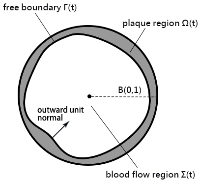
Figure 1. The cross section of an artery.

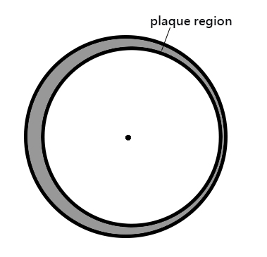
Figure 2. A symmetry-breaking solution in the $n=1$ bifurcation branch

For the system $($1.1$)$ – $($1.14$)$, Friedman et al. [6] studied the radially symmetric case and justified the existence of a unique radially symmetric steady state solution in a small ring-region $1-\varepsilon\leq r\leq 1$, which describes the arterial plaque in the early stage of atherosclerosis. Later on Zhao and Hu [10] carried out the bifurcation analysis for the system and established a branch of bifurcation points for $n\geq 2$. More specifically, they used $\mu=\frac{1}{\varepsilon}[\lambda L_{0}-\rho_{3}(\gamma+H_{0})]$ as the bifurcation parameter, and showed that for $n\geq 2$, there exists a unique

(1.15) $$\mu_{n}=(\gamma+H_{0})n^{2}(1-n^{2})+O(n^{5}\varepsilon),$$

if $\mu_{n}>\mu_{c}$ ($\mu_{c}$ is defined in equation (2.9) in [10]), then $\mu=\mu_{n}$ is a bifurcation point of the symmetry-breaking stationary solution when $\varepsilon$ is small enough.

Based on further exploration and refinements of the estimates in [10], we shall prove in this paper that $\mu_{1}=O(\varepsilon)$ is also a bifurcation point for the system $($1.1$)$ – $($1.14$)$ by verifying the Crandall-Rabinowitz Theorem (Theorem 2.2). Our main result is stated in the following theorem.

Theorem 1.1.

Assume that $\mu_{c}<0$ and $\beta_{1}\neq\beta_{2}$. For $\mu_{1}=O(\varepsilon)$ defined as the solution to the equation $($2.35$)$ with $n=1$, we can find a small $E>0$, such that for $0<\varepsilon<E$, then $\mu=\mu_{1}$ is a bifurcation point of the symmetry-breaking stationary solution for the system $($1.1$)$ – $($1.14$)$. Moreover, the free boundary of this bifurcation solution is of the form

(1.16) $$r=1-\varepsilon+\tau\cos(\theta)+o(\tau),\hskip 20.00003pt\text{where }|\tau|\ll\varepsilon.$$

In recent years, considerable research works have been done on bifurcation analysis based upon the Crandall-Rabinowitz Theorem (see [12, 13, 14, 15, 16, 17, 18, 19, 20, 21, 22, 23, 24, 25]). In these works, the solutions on the $n=1$ bifurcation branch are just $\varepsilon$-translations of the origin of the radially symmetric solution; after transformation of coordinates, this kind of solutions are still radially symmetric. Therefore, the $n=1$ case is always ignored in previous works on the bifurcation analysis. For our problem, however, the circumstances are very different. There are two boundaries for the system $($1.1$)$ – $($1.14$)$, with the outer boundary $r=1$ being fixed. Since the outer boundary is fixed, all the perturbations make changes only on the inner free boundary. Due to this special geometry, the solutions on the $n=1$ bifurcation branch are non-radially symmetric, as shown in the Figure 2.

We want to emphasise that, for technical reasons, Theorem 1.1 was not established in [10]. The primary reason is that, by $($1.15$)$, both $\mu_{0}$ and $\mu_{1}$ are of order $O(\varepsilon)$; thus $($1.15$)$ is not enough to guarantee $\mu_{0}\neq\mu_{1}$, and hence the assumption (2) of the Crandall-Rabinowitz Theorem cannot be verified. The main goal of this paper is to derive more sophisticated estimates for $\mu_{0}$ and $\mu_{1}$, with which we can then verify the Crandall-Rabinowitz Theorem.

From mathematical point of view, $\mu=\mu_{1}=O(\varepsilon)$ is the first bifurcation point, which often coincides with the change of stability for the system. In fact, it has been proved in [6] that the radially symmetric plaque would disappear if $\mu<0$, and remain persistent if $\mu>0$; hence it is likely that the stability of the radially symmetric solution would change around $\mu=0$. More importantly, $\mu=\mu_{1}=O(\varepsilon)$ is also the most significant bifurcation point biologically, as the arterial plaque is often accumulated more on one side of the artery in reality (see Figures in [26, 27, 28]).

The structure of this paper is as follows. We collect some preliminaries in Section 2, and give some useful estimates in Section 3. The proof to the main result, Theorem 1.1, is presented in Section 4.

2. Preliminaries

2.1. A small radially symmetric stationary solution

We denote the radially symmetric stationary solution of the system $($1.1$)$ – $($1.14$)$ by $(L_{*},H_{*},F_{*},p_{*})$. Dropping all the time derivatives, and writing the system in polar coordinates in the domain $\Omega_{*}=\{1-\varepsilon<r<1\}$, we obtain the equation for $(L_{*},H_{*},F_{*},p_{*})$:

(2.1) $$-\Delta L_{*}=-k_{1}\frac{(M_{0}-F_{*})L_{*}}{K_{1}+L_{*}}-\rho_{1}L_{*} \text{in }\Omega_{*},$$

(2.2) $$-\Delta H_{*}=-k_{2}\frac{H_{*}F_{*}}{K_{2}+F_{*}}-\rho_{2}H_{*} \text{in }\Omega_{*},$$

(2.3) $$-D\Delta F_{*}-\frac{\partial F_{*}}{\partial r}\frac{\partial p_{*}}{\partial r}=k_{1}\frac{(M_{0}-F_{*})L_{*}}{K_{1}+L_{*}}-k_{2}\frac{H_{*}F_{*}}{K_{2}+F_{*}}-\lambda\frac{F_{*}(M_{0}-F_{*})L_{*}}{M_{0}(\gamma+H_{*})}+(\rho_{3}-\rho_{4})\frac{(M_{0}-F_{*})F_{*}}{M_{0}} \text{in }\Omega_{*},$$

(2.4) $$-\Delta p_{*}=\frac{1}{M_{0}}\Big{[}\lambda\frac{(M_{0}-F_{*})L_{*}}{\gamma+H_{*}}-\rho_{3}(M_{0}-F_{*})-\rho_{4}F_{*}\Big{]}\hskip 10.00002pt \text{in }\Omega_{*},$$

(2.5) $$\frac{\partial L_{*}}{\partial r}=\frac{\partial H_{*}}{\partial r}=\frac{\partial F_{*}}{\partial r}=\frac{\partial p_{*}}{\partial r}=0,\hskip 20.00003pt r=1,$$

(2.6) $$\hskip 10.00002pt-\frac{\partial L_{*}}{\partial r}+\beta_{1}(L_{*}-L_{0})=0,\hskip 10.00002pt-\frac{\partial H_{*}}{\partial r}+\beta_{1}(H_{*}-H_{0})=0,\hskip 10.00002pt-\frac{\partial F_{*}}{\partial r}+\beta_{2}F_{*}=0,\hskip 10.00002pt r=1-\varepsilon,$$

(2.7) $$p_{*}=-\frac{1}{1-\varepsilon},\hskip 10.00002pt r=1-\varepsilon,$$

(2.8) $$\frac{\partial p_{*}}{\partial r}=0, r=1-\varepsilon.$$

There are many parameters in the system. As in [10], we keep all parameters fixed except $L_{0}$ and $\rho_{4}$. For convenience, rather than using $L_{0}$, we use $\mu=\frac{1}{\varepsilon}[\lambda L_{0}-\rho_{3}(\gamma+H_{0})]$ as our bifurcation parameter and let $\rho_{4}=\rho_{4}(\mu)$. The existence theorem for the radially symmetric solution has been established in [10], and is stated as follows:

Theorem 2.1.

Define $\mu_{c}=\frac{\rho_{3}}{\beta_{1}}\Big{\{}(\gamma+H_{0})\Big{(}\frac{\lambda k_{1}M_{0}}{\lambda K_{1}+\rho_{3}(\gamma+H_{0})}+{\rho_{1}}\Big{)}-\rho_{2}H_{0}\Big{\}}$, for every $\mu_{*}>\mu_{c}$ and $\mu_{c}<\mu<\mu_{*}$, we can find a small $\varepsilon^{*}>0$, and for each $0<\varepsilon<\varepsilon^{*}$, there exists a unique $\rho_{4}$ such that the system $($2.1$)$ – $($2.8$)$ admits a unique solution $(L_{*},H_{*},F_{*},p_{*})$.

Remark 2.1.

By ODE theories, the solution $(L_{*},H_{*},F_{*},p_{*})$ can be extended to the bigger region $\Omega_{2\varepsilon}=\{1-2\varepsilon<r<1\}$ while maintaining $C^{\infty}$ regularity. For notational convenience, we still use $(L_{*},H_{*},F_{*},p_{*})$ to denote the extended solution.

2.2. Bifurcation theorem

Next we state a useful theorem which is critical in studying bifurcations.

Theorem 2.2.

(Crandall-Rabinowitz theorem, [29]) Let $X$, $Y$ be real Banach spaces and $\mathcal{F}(\cdot,\cdot)$ a $C^{p}$ map, $p\geq 3$, of a neighborhood $(0,\mu_{0})$ in $X\times\mathbb{R}$ into $Y$. Suppose

• $\mathcal{F}(0,\mu)=0$ for all $\mu$ in a neighborhood of $\mu_{0}$,

• $\mathrm{Ker}\,\mathcal{F}_{x}(0,\mu_{0})$ is one dimensional space, spanned by $x_{0}$,

• $\mathrm{Im}\,\mathcal{F}_{x}(0,\mu_{0})=Y_{1}$ has codimension 1,

• $\mathcal{F}_{\mu x}(0,\mu_{0})x_{0}\notin Y_{1}$.

Then $(0,\mu_{0})$ is a bifurcation point of the equation $\mathcal{F}(x,\mu)=0$ in the following sense: In a neighborhood of $(0,\mu_{0})$ the set of solutions $\mathcal{F}(x,\mu)=0$ consists of two $C^{p-2}$ smooth curves $\Gamma_{1}$ and $\Gamma_{2}$ which intersect only at the point $(0,\mu_{0})$; $\Gamma_{1}$ is the curve $(0,\mu)$ and $\Gamma_{2}$ can be parameterized as follows:

$$\Gamma_{2}:(x(\varepsilon),\mu(\varepsilon)),|\varepsilon|\text{ small, }(x(0),\mu(0))=(0,\mu_{0}),\;x^{\prime}(0)=x_{0}.$$

2.3. Preparations for the bifurcation theorem

In order to tackle the existence of symmetry-breaking stationary solutions to system $($1.1$)$ – $($1.14$)$, we’d like to apply the Crandall-Rabinowitz theorem. The preparations are the same as in [10], and are similar as those in [12, 13, 14, 15, 16, 17, 18, 19, 20, 21, 22, 23, 24, 25].

We consider a family of perturbed domains $\Omega_{\tau}=\{1-\varepsilon+\widetilde{R}<r<1\}$ and denote the corresponding inner boundary to be $\Gamma_{\tau}$, where $\widetilde{R}=\tau S(\theta)$, $|\tau|\ll\varepsilon$ and $|S|\leq 1$. Let $(L,H,F,p)$ be the solution of the system:

(2.9) $$-\Delta L=-k_{1}\frac{(M_{0}-F)L}{K_{1}+L}-\rho_{1}L\hskip 10.00002pt \text{in }\Omega_{\tau},$$

(2.10) $$-\Delta H=-k_{2}\frac{HF}{K_{2}+F}-\rho_{2}H\hskip 10.00002pt \text{in }\Omega_{\tau},$$

(2.11) $$-D\Delta F-\nabla F\cdot\nabla p=k_{1}\frac{(M_{0}-F)L}{K_{1}+L}-k_{2}\frac{HF}{K_{2}+F}-\lambda\frac{F(M_{0}-F)L}{M_{0}(\gamma+H)}+(\rho_{3}-\rho_{4})\frac{(M_{0}-F)F}{M_{0}}\hskip 10.00002pt \text{in }\Omega_{\tau},$$

(2.12) $$-\Delta p=\frac{1}{M_{0}}\Big{[}\lambda\frac{(M_{0}-F)L}{\gamma+H}-\rho_{3}(M_{0}-F)-\rho_{4}F\Big{]}\hskip 10.00002pt \text{in }\Omega_{\tau},$$

(2.13) $$\frac{\partial L}{\partial r}=\frac{\partial H}{\partial r}=\frac{\partial F}{\partial r}=\frac{\partial p}{\partial r}=0,\hskip 20.00003pt r=1,$$

(2.14) $$\frac{\partial L}{\partial{\bf n}}+\beta_{1}(L-L_{0})=0,\hskip 10.00002pt\frac{\partial H}{\partial{\bf n}}+{\beta_{1}}(H-H_{0})=0,\hskip 10.00002pt\frac{\partial F}{\partial{\bf n}}+\beta_{2}F=0 \text{on }\Gamma_{\tau},$$

(2.15) $$p=\kappa \text{on }\Gamma_{\tau}.$$

The existence and uniqueness of such a solution is guaranteed in [10]. We then define function $\mathcal{F}$ by

(2.16) $$\mathcal{F}(\tau S,\mu)=-\frac{\partial p}{\partial{\bf n}}\Big{|}_{\Gamma_{\tau}},$$

We know that $(L,H,F,p)$ is a symmetry-breaking stationary solution if and only if $\mathcal{F}(\tau S,\mu)=0$. Next we introduce the Banach spaces:

$$X^{l+\alpha}=\{S\in C^{l+\alpha}(\Sigma),S\text{ is $2\pi$-periodic in $\theta$}\},$$

(2.17) $$X^{l+\alpha}_{1}=\text{closure of the linear space spanned by $\{\cos(n\theta),n=0,1,2,\cdots\}$ in $X^{l+\alpha}$}.$$

It has been shown in [10] that the mapping $\mathcal{F}(\cdot,\mu):X^{l+4+\alpha}_{1}\rightarrow X^{l+1+\alpha}_{1}$ is bounded for any $l>0$.

In order to apply the Crandall-Rabinowitz theorem, we need to compute the Fréchet derivatives of $\mathcal{F}$. For a fixed small $\varepsilon$, we write the expansion of $(L,H,F,p)$ of order $\tau$ as follows:

(2.18) $$L=L_{*}+\tau L_{1}+O(\tau^{2}),$$

(2.19) $$H=H_{*}+\tau H_{1}+O(\tau^{2}),$$

(2.20) $$F=F_{*}+\tau F_{1}+O(\tau^{2}),$$

(2.21) $$p=p_{*}+\tau p_{1}+O(\tau^{2}).$$

The rigorous justification for $($2.18$)$ – $($2.21$)$ can be found in [10]. Substituting $($2.18$)$ – $($2.21$)$ into $($2.9$)$ – $($2.15$)$, and dropping all the higher order terms in $\tau$, we obtain the system for $(L_{1},H_{1},F_{1},p_{1})$, which is also called the linearized system of $($2.9$)$ – $($2.15$)$.

Set the perturbation $S(\theta)=\cos(n\theta)$, we are seeking solutions of the form

(2.22) $$L_{1}=L_{1}^{n}\cos(n\theta),\hskip 20.00003pt H_{1}=H_{1}^{n}\cos(n\theta),$$

(2.23) $$F_{1}=F_{1}^{n}\cos(n\theta),\hskip 20.00003pt p_{1}=p_{1}^{n}\cos(n\theta).$$

From [10, (4.7)-(4.16)], we know that the equations for $(L_{1}^{n},H_{1}^{n},F_{1}^{n},p_{1}^{n})$ are (Recall that $\Omega_{*}$ denotes the annulus $1-\varepsilon\leq r\leq 1$):

(2.24) $$-\frac{\partial^{2}L_{1}^{n}}{\partial r^{2}}-\frac{1}{r}\frac{\partial L_{1}^{n}}{\partial r}+\frac{n^{2}}{r^{2}}L_{1}^{n}=f_{5}(L_{1}^{n},H_{1}^{n},F_{1}^{n})\hskip 20.00003pt \text{in }\Omega_{*},$$

(2.25) $$-\frac{\partial^{2}H_{1}^{n}}{\partial r^{2}}-\frac{1}{r}\frac{\partial H_{1}^{n}}{\partial r}+\frac{n^{2}}{r^{2}}H_{1}^{n}=f_{6}(L_{1}^{n},H_{1}^{n},F_{1}^{n})\hskip 20.00003pt \text{in }\Omega_{*},$$

(2.26) $$-\frac{\partial^{2}F_{1}^{n}}{\partial r^{2}}-\frac{1}{r}\frac{\partial F_{1}^{n}}{\partial r}+\frac{n^{2}}{r^{2}}F_{1}^{n}=\frac{1}{D}\Big{(}f_{7}(L_{1}^{n},H_{1}^{n},F_{1}^{n})+\frac{\partial F_{*}}{\partial r}\frac{\partial p_{1}^{n}}{\partial r}+\frac{\partial F_{1}^{n}}{\partial r}\frac{\partial p_{*}}{\partial r}\Big{)}\hskip 20.00003pt \text{in }\Omega_{*},$$

(2.27) $$-\frac{\partial^{2}p_{1}^{n}}{\partial r^{2}}-\frac{1}{r}\frac{\partial p_{1}^{n}}{\partial r}+\frac{n^{2}}{r^{2}}p_{1}^{n}=f_{8}(L_{1}^{n},H_{1}^{n},F_{1}^{n})\hskip 20.00003pt \text{in }\Omega_{*},$$

(2.28) $$\frac{\partial L_{1}^{n}}{\partial r}=\frac{\partial H_{1}^{n}}{\partial r}=\frac{\partial F_{1}^{n}}{\partial r}=\frac{\partial p_{1}^{n}}{\partial r}=0 r=1,$$

(2.29) $$-\frac{\partial L_{1}^{n}}{\partial r}+\beta_{1}L_{1}^{n}=\Big{(}\frac{\partial^{2}L_{*}}{\partial r^{2}}-\beta_{1}\frac{\partial L_{*}}{\partial r}\Big{)}\Big{|}_{r=1-\varepsilon} r=1-\varepsilon,$$

(2.30) $$-\frac{\partial H_{1}^{n}}{\partial r}+\beta_{1}H_{1}^{n}=\Big{(}\frac{\partial^{2}H_{*}}{\partial r^{2}}-\beta_{1}\frac{\partial H_{*}}{\partial r}\Big{)}\Big{|}_{r=1-\varepsilon} r=1-\varepsilon,$$

(2.31) $$-\frac{\partial F_{1}^{n}}{\partial r}+\beta_{2}F_{1}^{n}=\Big{(}\frac{\partial^{2}F_{*}}{\partial r^{2}}-\beta_{2}\frac{\partial F_{*}}{\partial r}\Big{)}\Big{|}_{r=1-\varepsilon} r=1-\varepsilon,$$

(2.32) $$p_{1}^{n}=\frac{1-n^{2}}{(1-\varepsilon)^{2}} r=1-\varepsilon,$$

where $f_{5},f_{6},f_{7},$ and $f_{8}$ can all be bounded by linear functions of $|L_{1}^{n}|$, $|H_{1}^{n}|$, and $|F_{1}^{n}|$. In particular, $f_{8}$ is expressed as

(2.33) $$f_{8}(L_{1}^{n},H_{1}^{n},F_{1}^{n})=\frac{1}{M_{0}}\Big{[}\lambda\frac{(M_{0}-F_{*})L^{n}_{1}}{\gamma+H_{*}}-\lambda\frac{L_{*}F^{n}_{1}}{\gamma+H_{*}}-\lambda\frac{(M_{0}-F_{*})L_{*}H^{n}_{1}}{(\gamma+H_{*})^{2}}+(\rho_{3}-\rho_{4})F_{1}^{n}\Big{]},$$

Since $\mathcal{F}(0,\mu)=\frac{\partial p_{*}}{\partial r}\big{|}_{r=1-\varepsilon}=0$ by $($2.8$)$, we can utilize the expansions $($2.18$)$ – $($2.21$)$ to derive (more rigorous proof can be found in [10])

$$\mathcal{F}(\tau S,\mu)-\mathcal{F}(0,\mu)=-\frac{\partial p}{\partial{\bm{n}}}\Big{|}_{\Gamma_{\tau}} =\frac{\partial(p_{*}+\tau p_{1})}{\partial r}\Big{|}_{r=1-\varepsilon+\tau S}+O(|\tau|^{2}\|S\|_{C^{4+\alpha}(\Sigma)})$$

$$=\tau\Big{[}\frac{\partial^{2}p_{*}}{\partial r^{2}}\Big{|}_{r=1-\varepsilon}S(\theta)+\frac{\partial p_{1}}{\partial r}\Big{|}_{r=1-\varepsilon}\Big{]}+O(|\tau|^{2}\|S\|_{C^{4+\alpha}(\Sigma)}),$$

which leads to the Fréchet derivative of $\mathcal{F}$ at $(0,\mu)$ as below

$$\Big{[}\mathcal{F}_{\widetilde{R}}(0,\mu)\Big{]}S(\theta)=\frac{\partial^{2}p_{*}}{\partial r^{2}}\Big{|}_{r=1-\varepsilon}S(\theta)+\frac{\partial p_{1}}{\partial r}\Big{|}_{r=1-\varepsilon}.$$

Substituting in $S(\theta)=\cos(n\theta)$ and $($2.23$)$, we further obtain

(2.34) $$[\mathcal{F}_{\widetilde{R}}(0,\mu)]\cos(n\theta)=\Big{(}\frac{\partial^{2}p_{*}(1-\varepsilon)}{\partial r^{2}}+\frac{\partial p_{1}^{n}(1-\varepsilon)}{\partial r}\Big{)}\cos(n\theta).$$

Therefore we denote $\mu=\mu_{n}$ to be the solution to the equation

(2.35) $$\frac{\partial^{2}p_{*}(1-\varepsilon)}{\partial r^{2}}+\frac{\partial p_{1}^{n}(1-\varepsilon)}{\partial r}=0.$$

Clearly, for each $n\geq 0$, $[\mathcal{F}_{\widetilde{R}}(0,\mu)]\cos(n\theta)=0$ if and only if $\mu=\mu_{n}$. It is shown that for $n\geq 2$, $\mu=\mu_{n}$ is a bifurcation point.

3. Useful Estimates and Lemmas

A lot of estimates were derived in [10]. In order to derive a better estimates than $($1.15$)$ for $n=0$ and $1$, here we collect some of them (i.e., (2.11)–(2.13) and (4.47)–(4.52)) which will be useful in this paper. (Note that we only consider the cases when $n=0$ and 1, hence we don’t need the order of $n$ in higher order terms of $\varepsilon$.)

$$L_{*}(r) = L_{0}-\frac{\varepsilon}{\beta_{1}}\Big{(}\frac{k_{1}M_{0}L_{0}}{K_{1}+L_{0}}+\rho_{1}L_{0}\Big{)}+O(\varepsilon^{2})$$

$$= \frac{\rho_{3}(\gamma+H_{0})}{\lambda}+\varepsilon\Big{[}\frac{\mu}{\lambda}-\frac{\rho_{3}(\gamma+H_{0})}{\beta_{1}}\Big{(}\frac{k_{1}M_{0}}{\lambda K_{1}+\rho_{3}(\gamma+H_{0})}+\frac{\rho_{1}}{\lambda}\Big{)}\Big{]}+O(\varepsilon^{2})$$

$$\triangleq \frac{\rho_{3}(\gamma+H_{0})}{\lambda}+\varepsilon L_{*}^{1}+O(\varepsilon^{2}),$$

(3.2) $$H_{*}(r) = H_{0}-\varepsilon\frac{\rho_{2}H_{0}}{\beta_{1}}+O(\varepsilon^{2})\;\triangleq\;H_{0}+\varepsilon H_{*}^{1}+O(\varepsilon^{2}),$$

$$F_{*}(r) = \frac{\varepsilon}{\beta_{2}}\frac{k_{1}M_{0}L_{0}}{D(K_{1}+L_{0})}+O(\varepsilon^{2})$$

$$= \varepsilon\;\frac{\rho_{3}(\gamma+H_{0})}{\beta_{2}D}\;\frac{k_{1}M_{0}}{\lambda K_{1}+\rho_{3}(\gamma+H_{0})}+O(\varepsilon^{2})\;\triangleq\;\varepsilon F_{*}^{1}+O(\varepsilon^{2}).$$

(3.4) $$L_{1}^{n}(r) = \frac{1}{\beta_{1}}\Big{(}\frac{\partial^{2}L_{*}}{\partial r^{2}}-\beta_{1}\frac{\partial L_{*}}{\partial r}\Big{)}\Big{|}_{r=1-\varepsilon}+O(\varepsilon)\;=\;\frac{\mu}{\lambda}-L_{*}^{1}+O(\varepsilon),$$

(3.5) $$H_{1}^{n}(r) = \frac{1}{\beta_{1}}\Big{(}\frac{\partial^{2}H_{*}}{\partial r^{2}}-\beta_{1}\frac{\partial H_{*}}{\partial r}\Big{)}\Big{|}_{r=1-\varepsilon}+O(\varepsilon)\;=\;-H_{*}^{1}+O(\varepsilon),$$

(3.6) $$F_{1}^{n}(r) = \frac{1}{\beta_{2}}\Big{(}\frac{\partial^{2}F_{*}}{\partial r^{2}}-\beta_{2}\frac{\partial F_{*}}{\partial r}\Big{)}\Big{|}_{r=1-\varepsilon}+O(\varepsilon)\;=\;-F_{*}^{1}+O(\varepsilon).$$

The following lemma is from [10] (Lemma 2.2). It includes a relationship among the parameters, which will be used later.

Lemma 3.1.

For the radially symmetric stationary solution $(L_{*},H_{*},F_{*},p_{*})$, the following estimates holds

(3.7) $$\frac{M_{0}(\lambda L_{*}^{1}-\rho_{3}H_{*}^{1})}{\gamma+H_{0}}-\rho_{4}F_{*}^{1}=O(\varepsilon),$$

in other words, $\rho_{4}$ can be expressed as

(3.8) $$\rho_{4}=\frac{1}{F_{*}^{1}}\,\frac{M_{0}}{\gamma+H_{0}}(\lambda L_{*}^{1}-\rho_{3}H_{*}^{1})+O(\varepsilon).$$

Notice that equations $($2.24$)$ – $($2.27$)$ are of similar structure, hence we denote the operator $\mathscript L_{n}\triangleq\frac{\partial^{2}}{\partial r^{2}}+\frac{1}{r}\frac{\partial}{\partial r}+\frac{n^{2}}{r^{2}}$. For this special operator, one can easily verify the following lemmas (special case of $n=0$ and $1$ in [10, Lemma 4.2], with the case $n=1$ modified to satisfy $\psi_{1}(1)=\psi_{1}^{\prime}(1)=0$)

Lemma 3.2.

The general solution of ($\eta$ is a constant)

(3.9) $${\mathscript L}_{n}[\psi]\triangleq-\psi^{\prime\prime}-\frac{1}{r}\psi^{\prime}+\frac{n^{2}}{r^{2}}\psi=\eta+f(r)\hskip 20.00003pt1-\varepsilon<r<1,$$

$$\psi^{\prime}(1)=0,$$

is given by

(3.12) $$\psi-\psi_{1}=\left\{\begin{array}[]{ll}\displaystyle Ar+\frac{1}{r}\Big{(}A+K[f]^{\prime}(1)\Big{)}+K[f](r)&n=1,\\ A+K[f](r)&n=0,\end{array}\right.$$

where

(3.15) $$K[f](r)=\left\{\begin{array}[]{ll}\displaystyle\frac{r}{2}\int_{r}^{1}f(s)\,\mathrm{d}s+\frac{r^{-1}}{2}\int_{1-\varepsilon}^{r}s^{2}f(s)\,\mathrm{d}s&n=1,\\ \displaystyle\rule{0.0pt}{18.0pt}-\int_{r}^{1}\Big{(}\log\frac{s}{r}\Big{)}\;sf(s)\,\mathrm{d}s&n=0;\end{array}\right.$$

in addition, $\psi_{1}(r)$ satisfies

(3.16) $${\mathscript L}_{n}[\psi_{1}]=-\psi_{1}^{\prime\prime}-\frac{1}{r}\psi_{1}^{\prime}+\frac{n^{2}}{r^{2}}\psi_{1}=\eta\hskip 20.00003pt1-\varepsilon<r<1,$$

$$\psi_{1}^{\prime}(1)=0,\hskip 20.00003pt\psi_{1}(1)=0,$$

and is given by

(3.20) $$\psi_{1}=\left\{\begin{array}[]{ll}\displaystyle\eta\Big{(}-\frac{1}{6r}+\frac{1}{2}r-\frac{1}{3}r^{2}\Big{)}&n=1,\\ \vspace{-8pt}\\ \displaystyle\eta\Big{(}\frac{1-r^{2}}{4}+\frac{1}{2}\log r\Big{)}&n=0.\end{array}\right.$$

The special solution $K[f]$ satisfies

(3.21) $$|K[f](r)|\leq\frac{\varepsilon}{2}\|f\|_{L^{\infty}},\hskip 20.00003pt|K[f]^{\prime}(r)|\leq\frac{\varepsilon}{2}\|f\|_{L^{\infty}},\hskip 20.00003ptn=1,$$

and

(3.22) $$|K[f](r)|\leq\varepsilon\|f\|_{L^{\infty}},\hskip 20.00003pt|K[f]^{\prime}(r)|\leq\varepsilon\|f\|_{L^{\infty}},\hskip 20.00003ptn=0.$$

The proof is the same as in [10]. We add one more restriction on $\psi_{1}$, i.e., $\psi_{1}(1)=0$, but it doesn’t affect the proof. Since $\psi_{1}(1)=\psi_{1}^{\prime}(1)=0$, and by $($3.16$)$,

$$\psi_{1}^{\prime\prime}(1)=-\eta+\Big{(}-\frac{1}{r}\psi_{1}^{\prime}+\frac{n^{2}}{r^{2}}\psi_{1}\Big{)}\Big{|}_{r=1}=-\eta.$$

In addition, differentiating the equation $($3.16$)$ and evaluating at $r=1$, we further obtain

$$\psi_{1}^{\prime\prime\prime}(1)=\Big{(}-\frac{r\psi_{1}^{\prime\prime}-\psi_{1}^{\prime}}{r^{2}}+n^{2}\frac{r^{2}\psi_{1}^{\prime}-2r\psi_{1}}{r^{4}}\Big{)}\Big{|}_{r=1}=-\psi_{1}^{\prime\prime}(1)=\eta.$$

Based on the above two equations, it then follows from the Taylor series that, for $1-\varepsilon\leq r\leq 1$,

(3.23) $$\psi_{1}(r)=\psi_{1}(1)+\psi_{1}^{\prime}(1)(r-1)+\frac{\psi_{1}^{\prime\prime}(1)}{2}(r-1)^{2}+\cdots=-\frac{\eta}{2}(r-1)^{2}+O(\varepsilon^{3}),$$

(3.24) $$\psi_{1}^{\prime}(r)=\psi_{1}^{\prime}(1)+\psi_{1}^{\prime\prime}(1)(r-1)+\frac{\psi_{1}^{\prime\prime\prime}(1)}{2}(r-1)^{2}+\cdots=-\eta(r-1)+\frac{\eta}{2}(r-1)^{2}+O(\varepsilon^{3}).$$

In particular, we have

(3.25) $$\psi_{1}(1-\varepsilon)=-\frac{\eta}{2}\varepsilon^{2}+O(\varepsilon^{3}),$$

(3.26) $$\psi_{1}^{\prime}(1-\varepsilon)=\varepsilon\eta+\frac{\eta}{2}\varepsilon^{2}+O(\varepsilon^{3}).$$

Lemma 3.3.

If in addition to $($3.9$)$, we further assume the boundary condition

(3.27) $$-\psi^{\prime}(1-\varepsilon)+\beta\psi(1-\varepsilon)=G,$$

then the coefficient $A$ in $($3.12$)$ can be explicitly computed as: for $n=1$

(3.28) $$A=\frac{G+\psi_{1}^{\prime}(1-\varepsilon)-\beta\psi_{1}(1-\varepsilon)-\beta K[f](1-\varepsilon)+K[f]^{\prime}(1-\varepsilon)-\frac{1}{(1-\varepsilon)^{2}}K[f]^{\prime}(1)-\frac{\beta}{1-\varepsilon}K[f]^{\prime}(1)}{-1+\frac{1}{(1-\varepsilon)^{2}}+\beta(1-\varepsilon)+\frac{\beta}{1-\varepsilon}},$$

and for $n=0$,

(3.29) $$A=\frac{1}{\beta}\Big{[}G+\psi_{1}^{\prime}(1-\varepsilon)-\beta\psi_{1}(1-\varepsilon)-\beta K[f](1-\varepsilon)+K[f]^{\prime}(1-\varepsilon)\Big{]}.$$

Lemma 3.4.

If $f(r)=O(\varepsilon)$ in $($3.9$)$, and the assumptions in Lemma 3.3 hold, then for $1-\varepsilon\leq r\leq 1$,

(3.30) $$\psi(r)=\frac{G}{\beta}+\varepsilon\Big{(}\frac{\eta}{\beta}-\frac{G}{\beta^{2}}\Big{)}+O(\varepsilon^{2})\hskip 20.00003ptn=1,$$

(3.31) $$\psi(r)=\frac{G}{\beta}+\varepsilon\frac{\eta}{\beta}+O(\varepsilon^{2})\hskip 56.00014ptn=0.$$

Proof.

Based on Lemma 3.2, if $f(r)=O(\varepsilon)$ in $($3.9$)$, we have in either $n=0$ or $n=1$ case,

$$K[f](r)=O(\varepsilon^{2}),\hskip 20.00003ptK[f]^{\prime}(r)=O(\varepsilon^{2}).$$

Substituting into $($3.28$)$ and $($3.29$)$, recalling also $($3.25$)$ and $($3.26$)$, we obtain

$$A=\frac{G+\varepsilon\eta+O(\varepsilon^{2})}{2(\beta+\varepsilon)+O(\varepsilon^{2})}=\frac{G}{2\beta}+\varepsilon\Big{(}\frac{\eta}{2\beta}-\frac{G}{2\beta^{2}}\Big{)}+O(\varepsilon^{2})\hskip 20.00003pt n=1,$$

$$A=\frac{G+\varepsilon\eta+O(\varepsilon^{2})}{\beta}=\frac{G}{\beta}+\varepsilon\frac{\eta}{\beta}+O(\varepsilon^{2})\hskip 20.00003pt n=0.$$

Since $A$ is the only coefficient in $($3.12$)$, we can now substitute the above expressions for $A$ into $($3.12$)$ to derive, for $1-\varepsilon\leq r\leq 1$,

$$\psi(r)=A\Big{(}r+\frac{1}{r}\Big{)}+O(\varepsilon^{2})=2A+O(\varepsilon^{2})=\frac{G}{\beta}+\varepsilon\Big{(}\frac{\eta}{\beta}-\frac{G}{\beta^{2}}\Big{)}+O(\varepsilon^{2})\hskip 20.00003pt n=1,$$

$$\psi(r)=A+O(\varepsilon^{2})=\frac{G}{\beta}+\varepsilon\frac{\eta}{\beta}+O(\varepsilon^{2})\hskip 20.00003pt n=0.$$

This completes the proof. ∎

Notice that in this lemma the difference between $n=1$ and $n=0$ cases starts from $O(\varepsilon)$ terms; furthermore, the difference in $O(\varepsilon)$ terms is $\varepsilon\frac{G}{\beta^{2}}$, which is determined only by $G$ and $\beta$.

Lemma 3.2, together with Lemmas 3.3 and 3.4, are applied to equations for $L_{1}^{n}$, $H_{1}^{n}$ and $F_{1}^{n}$. Notice that the boundary condition for $p_{1}^{n}$ is

$$p_{1}^{n}(1-\varepsilon)=\frac{1-n^{2}}{(1-\varepsilon)^{2}},$$

which is of a different form from $($3.27$)$, we hence need the following lemma that can be easily verified:

Lemma 3.5.

If in addition to $($3.9$)$, we further assume the boundary condition for $\psi$

(3.32) $$\psi(1-\varepsilon)=\frac{1-n^{2}}{(1-\varepsilon)^{2}},$$

then the coefficient $A$ in $($3.12$)$ is solved as

$$A=\frac{-\psi_{1}(1-\varepsilon)-K[f](1-\varepsilon)-\frac{1}{1-\varepsilon}K[f]^{\prime}(1)}{1-\varepsilon+\frac{1}{1-\varepsilon}}\hskip 20.00003pt n=1,$$

$$A=-\psi_{1}(1-\varepsilon)-K[f](1-\varepsilon)\hskip 20.00003pt n=0.$$

Lemma 3.6.

If $f(r)=O(\varepsilon^{2})$ in $($3.9$)$, and the assumptions in Lemma 3.5 hold, then for $n=0,1$ and $1-\varepsilon\leq r\leq 1$,

(3.33) $$\psi^{\prime}(1-\varepsilon)=\varepsilon\eta+\varepsilon^{2}\frac{\eta}{2}+O(\varepsilon^{3}).$$

Proof.

If $f=O(\varepsilon^{2})$ in $($3.9$)$, by Lemma 3.2 we have

$$K[f](r)=O(\varepsilon^{3}),\hskip 20.00003ptK[f]^{\prime}(r)=O(\varepsilon^{3}).$$

In order to estimate $\psi^{\prime}(1-\varepsilon)$, we differentiate $($3.12$)$ and evaluate the derivative at $r=1-\varepsilon$,

$$\psi^{\prime}(1-\varepsilon)=\psi_{1}^{\prime}(1-\varepsilon)+A-\frac{1}{(1-\varepsilon)^{2}}\Big{(}A+K[f]^{\prime}(1)\Big{)}+K[f]^{\prime}(1-\varepsilon)\hskip 20.00003pt n=1,$$

$$\psi^{\prime}(1-\varepsilon)=\psi_{1}^{\prime}(1-\varepsilon)+K[f]^{\prime}(1-\varepsilon)\hskip 20.00003pt n=0.$$

Combining with the expression of $A$ in Lemma 3.5, recalling also $($3.23$)$ – $($3.26$)$, we further derive $A=O(\varepsilon^{2})$, and in both cases,

$$\psi^{\prime}(1-\varepsilon)=\varepsilon\eta+\varepsilon^{2}\frac{\eta}{2}+O(\varepsilon^{3})\hskip 20.00003pt n=0,1,$$

which completes the proof. ∎

4. Proof of Theorem 1.1

As mentioned before, the key is to show $\mu_{0}\neq\mu_{1}$. Since they are the same on the order of $O(1)$, we shall derive higher order approximations for $\mu_{0}$ and $\mu_{1}$. Hence the estimates $($3.4$)$ – $($3.6$)$ for $L_{1}^{n}$, $H_{1}^{n}$ and $F_{1}^{n}$ are not enough for the purpose of this paper – we need more information about the higher order terms in $\varepsilon$. To do that, we denote

(4.1) $$L_{1}^{n} = \frac{\mu}{\lambda}-L_{*}^{1}+\varepsilon L_{11}^{n}+O(\varepsilon^{2}),$$

(4.2) $$H_{1}^{n} = -H_{*}^{1}+\varepsilon H_{11}^{n}+O(\varepsilon^{2}),$$

(4.3) $$F_{1}^{n} = -F_{*}^{1}+\varepsilon F_{11}^{n}+O(\varepsilon^{2}),$$

and we proceed to estimate $L_{11}^{n}$, $H_{11}^{n}$ and $F_{11}^{n}$ based on Lemmas 3.2, 3.3 and 3.4.

Recall first the equations for $L_{1}^{n}$, $H_{1}^{n}$ and $F_{1}^{n}$ are ($\Omega_{*}$ denotes the annulus $1-\varepsilon\leq r\leq 1$):

(4.4) $$-\frac{\partial^{2}L_{1}^{n}}{\partial r^{2}}-\frac{1}{r}\frac{\partial L_{1}^{n}}{\partial r}+\frac{n^{2}}{r^{2}}L_{1}^{n}=f_{5}(L_{1}^{n},H_{1}^{n},F_{1}^{n})\hskip 20.00003pt \text{in }\Omega_{*},$$

(4.5) $$-\frac{\partial^{2}H_{1}^{n}}{\partial r^{2}}-\frac{1}{r}\frac{\partial H_{1}^{n}}{\partial r}+\frac{n^{2}}{r^{2}}H_{1}^{n}=f_{6}(L_{1}^{n},H_{1}^{n},F_{1}^{n})\hskip 20.00003pt \text{in }\Omega_{*},$$

(4.6) $$-\frac{\partial^{2}F_{1}^{n}}{\partial r^{2}}-\frac{1}{r}\frac{\partial F_{1}^{n}}{\partial r}+\frac{n^{2}}{r^{2}}F_{1}^{n}=\frac{1}{D}\Big{(}f_{7}(L_{1}^{n},H_{1}^{n},F_{1}^{n})+\frac{\partial F_{*}}{\partial r}\frac{\partial p_{1}^{n}}{\partial r}+\frac{\partial F_{1}^{n}}{\partial r}\frac{\partial p_{*}}{\partial r}\Big{)}\hskip 20.00003pt \text{in }\Omega_{*},$$

(4.7) $$\frac{\partial L_{1}^{n}}{\partial r}=\frac{\partial H_{1}^{n}}{\partial r}=\frac{\partial F_{1}^{n}}{\partial r}=0 r=1,$$

(4.8) $$-\frac{\partial L_{1}^{n}}{\partial r}+\beta_{1}L_{1}^{n}=\Big{(}\frac{\partial^{2}L_{*}}{\partial r^{2}}-\beta_{1}\frac{\partial L_{*}}{\partial r}\Big{)}\Big{|}_{r=1-\varepsilon} r=1-\varepsilon,$$

(4.9) $$-\frac{\partial H_{1}^{n}}{\partial r}+\beta_{1}H_{1}^{n}=\Big{(}\frac{\partial^{2}H_{*}}{\partial r^{2}}-\beta_{1}\frac{\partial H_{*}}{\partial r}\Big{)}\Big{|}_{r=1-\varepsilon} r=1-\varepsilon,$$

(4.10) $$-\frac{\partial F_{1}^{n}}{\partial r}+\beta_{2}F_{1}^{n}=\Big{(}\frac{\partial^{2}F_{*}}{\partial r^{2}}-\beta_{2}\frac{\partial F_{*}}{\partial r}\Big{)}\Big{|}_{r=1-\varepsilon} r=1-\varepsilon.$$

For the right-hand sides of $($4.4$)$ – $($4.6$)$, we can write them as the form $\eta+O(\varepsilon)$, and we shall claim that $\eta$ is independent of $n$. In fact, we notice that the $O(1)$ terms of $L_{1}^{n}(r)$, $H_{1}^{n}(r)$ and $F_{1}^{n}(r)$ in $($3.4$)$ – $($3.6$)$ are constants, and are independent of $n$. Moreover, it has been proved in [10] that $\frac{\partial F_{*}}{\partial r},\frac{\partial p_{*}}{\partial r}=O(\varepsilon)$, and $\frac{\partial p_{1}^{n}}{\partial r},\frac{\partial F_{1}^{n}}{\partial r}$ are both bounded. Hence the extra two terms in $($4.6$)$, $\frac{\partial F_{*}}{\partial r}\frac{\partial p_{1}^{n}}{\partial r}$ and $\frac{\partial F_{1}^{n}}{\partial r}\frac{\partial p_{*}}{\partial r}$, do not affect the $O(1)$ term $\eta$.

Using Lemma 3.4, we find that the difference between $L_{1}^{1}(r)$ and $L_{r}^{0}(r)$ starts from $O(\varepsilon)$ terms. As a matter of fact, by $($3.30$)$, $($3.31$)$, and $($3.4$)$,

$$L_{1}^{1}-L_{1}^{0}=-\frac{\varepsilon}{\beta_{1}^{2}}\Big{(}\frac{\partial^{2}L_{*}}{\partial r^{2}}-\beta_{1}\frac{\partial L_{*}}{\partial r}\Big{)}\Big{|}_{r=1-\varepsilon}+O(\varepsilon^{2})=\frac{\varepsilon}{\beta_{1}}\Big{(}L_{*}^{1}-\frac{\mu}{\lambda}\Big{)}+O(\varepsilon^{2}).$$

From $($4.1$)$, $L_{1}^{1}=\frac{\mu}{\lambda}-L_{*}^{1}+\varepsilon L_{11}^{1}+O(\varepsilon^{2})$, and $L_{1}^{0}=\frac{\mu}{\lambda}-L_{*}^{1}+\varepsilon L_{11}^{0}+O(\varepsilon^{2})$; combining with the above equation, we further have

(4.11) $$L_{11}^{1}-L_{11}^{0}=\frac{1}{\beta_{1}}\Big{(}L_{*}^{1}-\frac{\mu}{\lambda}\Big{)}.$$

Similarly, we can derive

(4.12) $$H_{11}^{1}-H_{11}^{0}=\frac{1}{\beta_{1}}H_{*}^{1},$$

(4.13) $$F_{11}^{1}-F_{11}^{0}=\frac{1}{\beta_{2}}F_{*}^{1}.$$

Next we consider the equation for $p_{1}^{n}$:

(4.14) $$-\frac{\partial^{2}p_{1}^{n}}{\partial r^{2}}-\frac{1}{r}\frac{\partial p_{1}^{n}}{\partial r}+\frac{n^{2}}{r^{2}}p_{1}^{n}=f_{8}(L_{1}^{n},H_{1}^{n},F_{1}^{n})\hskip 20.00003pt\text{in }\Omega_{*},$$

(4.15) $$\frac{\partial p_{1}^{n}}{\partial r}(1)=0,\hskip 20.00003ptp_{1}^{n}(1-\varepsilon)=\frac{1-n^{2}}{(1-\varepsilon)^{2}},$$

where

(4.16) $$f_{8}(L_{1}^{n},H_{1}^{n},F_{1}^{n})=\frac{1}{M_{0}}\Big{[}\lambda\frac{(M_{0}-F_{*})L^{n}_{1}}{\gamma+H_{*}}-\lambda\frac{L_{*}F^{n}_{1}}{\gamma+H_{*}}-\lambda\frac{(M_{0}-F_{*})L_{*}H^{n}_{1}}{(\gamma+H_{*})^{2}}+(\rho_{3}-\rho_{4})F_{1}^{n}\Big{]}.$$

In order to apply Lemmas 3.2, 3.5 and 3.6, we shall rewrite $f_{8}$ in the form $f_{8}=\eta+f(r)$, where $f(r)=O(\varepsilon^{2})$. More specifically, we denote,

$$f_{8}(L_{1}^{n},H_{1}^{n},F_{1}^{n})=\eta_{n}+O(\varepsilon^{2}),$$

and we now proceed a long and tedious journal to compute $\eta_{n}=\eta_{n}(\varepsilon)$. Substituting $($3$)$ – $($3$)$ and $($4.1$)$ – $($4.3$)$ all into $($4.16$)$, we have

$$M_{0}f_{8}\;= \;\lambda\frac{(M_{0}-\varepsilon F_{*}^{1})(\frac{\mu}{\lambda}-L_{*}^{1}+\varepsilon L_{11}^{n})}{\gamma+H_{0}+\varepsilon H_{*}^{1}}-\lambda\frac{(\frac{\rho_{3}(\gamma+H_{0})}{\lambda}+\varepsilon L_{*}^{1})(-F_{*}^{1}+\varepsilon F_{11}^{n})}{\gamma+H_{0}+\varepsilon H_{*}^{1}}+(\rho_{3}-\rho_{4})(-F_{*}^{1}+\varepsilon F_{11}^{n})$$

$$-\lambda\frac{(M_{0}-\varepsilon F_{*}^{1})(\frac{\rho_{3}(\gamma+H_{0})}{\lambda}+\varepsilon L_{*}^{1})(-H_{*}^{1}+\varepsilon H_{11}^{n})}{(\gamma+H_{0}+\varepsilon H_{*}^{1})^{2}}+O(\varepsilon^{2})$$

$$\;= \;\Big{(}\frac{M_{0}(\mu-\lambda L_{*}^{1})}{\gamma+H_{0}}+\frac{(-\varepsilon F_{*}^{1})(\mu-\lambda L_{*}^{1})}{\gamma+H_{0}}+\frac{\lambda M_{0}\varepsilon L_{11}^{n}}{\gamma+H_{0}}-\frac{M_{0}(\mu-\lambda L_{*}^{1})\varepsilon H_{*}^{1}}{(\gamma+H_{0})^{2}}\Big{)}-\Big{(}-\rho_{3}F_{*}^{1}-\frac{\lambda\varepsilon L_{*}^{1}F_{*}^{1}}{\gamma+H_{0}}$$

$$+\rho_{3}\varepsilon F_{11}^{n}+\frac{\rho_{3}F_{*}^{1}\varepsilon H_{*}^{1}}{\gamma+H_{0}}\Big{)}+\Big{(}-(\rho_{3}-\rho_{4})F_{*}^{1}+(\rho_{3}-\rho_{4})\varepsilon F_{11}^{n}\Big{)}-\Big{(}-\frac{M_{0}\rho_{3}H_{*}^{1}}{\gamma+H_{0}}+\frac{\varepsilon F_{*}^{1}\rho_{3}H_{*}^{1}}{\gamma+H_{0}}$$

$$-\frac{\lambda M_{0}\varepsilon L_{*}^{1}H_{*}^{1}}{(\gamma+H_{0})^{2}}+\frac{M_{0}\rho_{3}\varepsilon H_{11}^{n}}{\gamma+H_{0}}+\frac{2M_{0}\rho_{3}H_{*}^{1}\varepsilon H_{*}^{1}}{(\gamma+H_{0})^{2}}\Big{)}+O(\varepsilon^{2})$$

$$\;= \;\Big{(}\frac{M_{0}\mu}{\gamma+H_{0}}-\frac{M_{0}(\lambda L_{*}^{1}-\rho_{3}H_{*}^{1})}{\gamma+H_{0}}+\rho_{4}F_{*}^{1}\Big{)}+\varepsilon\Big{(}-\frac{F_{*}^{1}\mu}{\gamma+H_{0}}-\frac{M_{0}H_{*}^{1}\mu}{(\gamma+H_{0})^{2}}+2\frac{\lambda L_{*}^{1}F_{*}^{1}}{\gamma+H_{0}}+2\frac{\lambda M_{0}L_{*}^{1}H_{*}^{1}}{(\gamma+H_{0})^{2}}$$

$$-2\frac{\rho_{3}F_{*}^{1}H_{*}^{1}}{\gamma+H_{0}}-2\frac{M_{0}\rho_{3}(H_{*}^{1})^{2}}{(\gamma+H_{0})^{2}}\Big{)}+\varepsilon\Big{(}\frac{\lambda M_{0}L_{11}^{n}}{\gamma+H_{0}}-\frac{M_{0}\rho_{3}H_{11}^{n}}{\gamma+H_{0}}-\rho_{4}F_{11}^{n}\Big{)}+O(\varepsilon^{2}),$$

hence

(4.17) $$\eta_{n}= \;\frac{1}{M_{0}}\Big{[}\Big{(}\frac{M_{0}\mu}{\gamma+H_{0}}-\frac{M_{0}(\lambda L_{*}^{1}-\rho_{3}H_{*}^{1})}{\gamma+H_{0}}+\rho_{4}F_{*}^{1}\Big{)}+\varepsilon\Big{(}-\frac{F_{*}^{1}\mu}{\gamma+H_{0}}-\frac{M_{0}H_{*}^{1}\mu}{(\gamma+H_{0})^{2}}+2\frac{\lambda L_{*}^{1}F_{*}^{1}}{\gamma+H_{0}}$$

$$+2\frac{\lambda M_{0}L_{*}^{1}H_{*}^{1}}{(\gamma+H_{0})^{2}}-2\frac{\rho_{3}F_{*}^{1}H_{*}^{1}}{\gamma+H_{0}}-2\frac{M_{0}\rho_{3}(H_{*}^{1})^{2}}{(\gamma+H_{0})^{2}}\Big{)}\Big{]}+\frac{\varepsilon}{M_{0}}\Big{(}\frac{\lambda M_{0}L_{11}^{n}}{\gamma+H_{0}}-\frac{M_{0}\rho_{3}H_{11}^{n}}{\gamma+H_{0}}-\rho_{4}F_{11}^{n}\Big{)}.$$

We notice that all the terms in the first bracket of $($4.17$)$ are independent of $n$. Applying Lemma 3.6, we immediately have

(4.18) $$\frac{\partial p_{1}^{n}(1-\varepsilon)}{\partial r}=\varepsilon\eta_{n}+\varepsilon^{2}\frac{\eta_{n}}{2}+O(\varepsilon^{3}).$$

Now we are ready to prove our main result Theorem 1.1.

Proof of Theorem 1.1.

What we need to do is to verity the four assumptions of the Crandall-Rabinowitz Theorem (Theorem 2.2) at the point $\mu=\mu_{1}$. We choose the Banach spaces $X=X^{4+\alpha}_{1}$ and $Y=X^{1+\alpha}_{1}$. The differentiabilty of the map follows the same argument as in the papers [10, 18, 20, 24, 25]. To begin with, the assumption (1) is naturally satisfied, and the assumption (4) can be justified in the same way as in [10]. For the remaining assumptions (2) and (3), we need to prove

(4.19) $$\mu_{n}\neq\mu_{1}\hskip 20.00003pt\text{for }\forall n\neq 1.$$

From [10], it has been established that there exists a bound $E_{1}>0$, when $0<\varepsilon<E_{1}$, we have $\mu_{n}\neq\mu_{1}$ for each $n\geq 2$. Hence it suffices to show

(4.20) $$\mu_{0}\neq\mu_{1},$$

and we shall prove it by contradiction.

Recall that $\mu_{n}$ is the solution to the equation

$$\frac{\partial^{2}p_{*}(1-\varepsilon)}{\partial r^{2}}+\frac{\partial p_{1}^{n}(1-\varepsilon)}{\partial r}=0.$$

For the contrary, assuming $\mu_{0}=\mu_{1}$, we then have

(4.21) $$\frac{\partial p_{1}^{1}(1-\varepsilon)}{\partial r}-\frac{\partial p_{1}^{0}(1-\varepsilon)}{\partial r}=0.$$

On the other hand, it follows from $($4.18$)$ and $($4.17$)$ that

$$\frac{\partial p_{1}^{1}(1-\varepsilon)}{\partial r}-\frac{\partial p_{1}^{0}(1-\varepsilon)}{\partial r} =\;\varepsilon(\eta_{0}-\eta_{1})+\frac{\varepsilon^{2}}{2}(\eta_{0}-\eta_{1})+O(\varepsilon^{3})$$

$$=\;\frac{\varepsilon^{2}}{M_{0}}\Big{[}\frac{\lambda M_{0}}{\gamma+H_{0}}(L_{11}^{1}-L_{11}^{0})-\frac{\rho_{3}M_{0}}{\gamma+H_{0}}(H_{11}^{1}-H_{11}^{0})-\rho_{4}(F_{11}^{1}-F_{11}^{0})\Big{]}+O(\varepsilon^{3}).$$

Substituting into the estimates for $L_{11}^{1}-L_{11}^{0}$, $H_{11}^{1}-H_{11}^{0}$, and $F_{11}^{1}-F_{11}^{0}$ in $($4.11$)$ – $($4.13$)$, recalling also $($3.7$)$ in Lemma 3.1 and the fact that $\mu_{0},\mu_{1}=O(\varepsilon)$ by $($1.15$)$, we further have

$$\frac{\partial p_{1}^{1}(1-\varepsilon)}{\partial r}-\frac{\partial p_{1}^{0}(1-\varepsilon)}{\partial r} =\;\varepsilon^{2}\Big{[}\frac{\lambda}{\gamma+H_{0}}\frac{1}{\beta_{1}}(L_{*}^{1}-\frac{\mu_{0}}{\lambda})-\frac{\rho_{3}}{\gamma+H_{0}}\frac{H_{*}^{1}}{\beta_{1}}-\frac{\rho_{4}}{M_{0}}\frac{F_{*}^{1}}{\beta_{2}}\Big{]}+O(\varepsilon^{3})$$

$$=\;\varepsilon^{2}\Big{[}\frac{1}{\beta_{1}}\frac{\lambda L_{*}^{1}-\rho_{3}H_{*}^{1}}{\gamma+H_{0}}-\frac{1}{\beta_{2}}\frac{\rho_{4}F_{*}^{1}}{M_{0}}-\frac{\mu_{0}}{\beta_{1}(\gamma+H_{0})}\Big{]}+O(\varepsilon^{3})$$

$$=\;\varepsilon^{2}\Big{(}\frac{1}{\beta_{1}}-\frac{1}{\beta_{2}}\Big{)}\frac{\rho_{4}F_{*}^{1}}{M_{0}}+O(\varepsilon^{3}).$$

We have assumed that $\beta_{1}\neq\beta_{2}$. Since the sign of $\frac{\partial p_{1}^{1}(1-\varepsilon)}{\partial r}-\frac{\partial p_{1}^{0}(1-\varepsilon)}{\partial r}$ is dominated by $\Big{(}\frac{1}{\beta_{1}}-\frac{1}{\beta_{2}}\Big{)}\frac{\rho_{4}F_{*}^{1}}{M_{0}}$, we can easily find $E_{2}>0$, such that when $0<\varepsilon<E_{2}$,

$$\frac{\partial p_{1}^{1}(1-\varepsilon)}{\partial r}-\frac{\partial p_{1}^{0}(1-\varepsilon)}{\partial r}\neq 0,$$

which contradicts with the statement $($4.21$)$. Hence we have $\mu_{1}\neq\mu_{0}$ when $\varepsilon<E_{2}$.

By taking $E=\min\{E_{1},E_{2}\}$, we finish showing $($4.19$)$. With $($4.19$)$, we now have

$$\text{Ker}\,\mathcal{F}_{\widetilde{R}}(0,\mu_{1})=\text{span}\{\cos(\theta)\},$$

$$Y_{1}=\text{Im}\,\mathcal{F}_{\widetilde{R}}(0,\mu_{1})=\text{span}\{1,\cos(2\theta),\cos(3\theta),\cdots,\cos(n\theta),\cdots\},$$

$$Y_{1}\mbox{$\bigoplus$}\text{Ker}\,\mathcal{F}_{\widetilde{R}}(0,\mu_{1})=Y,$$

$$\left[\mathcal{F}_{\mu\widetilde{R}}(0,\mu_{1})\right]\in\text{span}\{\cos(\theta)\},\text{ and hence }\left[\mathcal{F}_{\mu\widetilde{R}}(0,\mu_{1})\right]\cos(\theta)\not\in Y_{1}.$$

In other words, all the spaces (kernel space, codimension space, non-tangential space) meet the requirements of the Crandall-Rabinowitz Theorem, and all the assumptions in the Crandall-Rabinowitz Theorem are satisfied. Therefore, $\mu=\mu_{1}$ is a bifurcation point for the system $($1.1$)$ – $($1.14$)$. ∎

References

[1]
Emelia J. Benjamin, Salim S. Virani, Clifton W. Callaway, Alanna M.
Chamberlain, Alexander R. Chang, Susan Cheng, Stephanie E. Chiuve, Mary
Cushman, Francesca N. Delling, Rajat Deo, Sarah D. de Ferranti, Jane F.
Ferguson, Myriam Fornage, Cathleen Gillespie, Carmen R. Isasi, Monik C.
Jiménez, Lori Chaffin Jordan, Suzanne E. Judd, Daniel Lackland, Judith H.
Lichtman, Lynda Lisabeth, Simin Liu, Chris T. Longenecker, Pamela L. Lutsey,
Jason S. Mackey, David B. Matchar, Kunihiro Matsushita, Michael E. Mussolino,
Khurram Nasir, Martin O’Flaherty, Latha P. Palaniappan, Ambarish Pandey,
Dilip K. Pandey, Mathew J. Reeves, Matthew D. Ritchey, Carlos J. Rodriguez,
Gregory A. Roth, Wayne D. Rosamond, Uchechukwu K.A. Sampson, Gary M. Satou,
Svati H. Shah, Nicole L. Spartano, David L. Tirschwell, Connie W. Tsao,
Jenifer H. Voeks, Joshua Z. Willey, John T. Wilkins, Jason HY. Wu, Heather M.
Alger, Sally S. Wong, and Paul Muntner.
Heart disease and stroke statistics-2018 update: a report from the
american heart association.
Circulation, 137(12):e67, 2018.
[2]Centers for Disease Control and Prevention and others.
Underlying cause of death, 1999-2013.
National Center for Health Statistics, Hyattsville, MD, 2015.
[3]
Vincent Calvez, Abderrhaman Ebde, Nicolas Meunier, and Annie Raoult.
Mathematical modelling of the atherosclerotic plaque formation.
In ESAIM: Proceedings, volume 28, pages 1–12. EDP Sciences,
2009.
[4]
Anna Cohen, Mary R Myerscough, and Rosemary S Thompson.
Athero-protective effects of high density lipoproteins (HDL): An
ODE model of the early stages of atherosclerosis.
Bulletin of mathematical biology, 76(5):1117–1142, 2014.
[5]
Avner Friedman and Wenrui Hao.
A mathematical model of atherosclerosis with reverse cholesterol
transport and associated risk factors.
Bulletin of mathematical biology, 77(5):758–781, 2015.
[6]
Avner Friedman, Wenrui Hao, and Bei Hu.
A free boundary problem for steady small plaques in the artery and
their stability.
Journal of Differential Equations, 259(4):1227–1255, 2015.
[7]
Wenrui Hao and Avner Friedman.
The LDL-HDL profile determines the risk of atherosclerosis: a
mathematical model.
PloS one, 9(3):e90497, 2014.
[8]
Cameron McKay, Sean McKee, Nigel Mottram, Tony Mulholland, Stephen Wilson,
Simon Kennedy, and Roger Wadsworth.
Towards a model of atherosclerosis.
University of Strathclyde, pages 1–29, 2005.
[9]
Debasmita Mukherjee, Lakshmi Narayan Guin, and Santabrata Chakravarty.
A reaction–diffusion mathematical model on mild atherosclerosis.
Modeling Earth Systems and Environment, pages 1–13, 2019.
[10]
Xinyue Evelyn Zhao and Bei Hu.
Symmetry-breaking bifurcation for a free boundary problem modeling
small arterial plaque.
preprint, 2020.
[12]
S. Cui and J. Escher.
Bifurcation analysis of an elliptic free boundary problem modelling
the growth of avascular tumors.
SIAM Journal on Mathematical Analysis, 39:210–235, 2007.
[13]
M. Fontelos and A. Friedman.
Symmetry-breaking bifurcations of free boundary problems in three
dimensions.
Asymptotic Analysis, 35:187–206, 2003.
[14]
Avner Friedman and Bei Hu.
Bifurcation from stability to instability for a free boundary problem
arising in a tumor model.
Archive for rational mechanics and analysis, 180(2):293–330,
2006.
[15]
A. Friedman and F. Reitich.
Symmetry-breaking bifurcation of analytic solutions to free boundary
problems: An application to a model of tumor growth.
Transactions of the American Mathematical Society,
353:1587–1634, 2000.
[16]
Wenrui Hao, Jonathan D Hauenstein, Bei Hu, and Andrew J Sommese.
A three-dimensional steady-state tumor system.
Applied Mathematics and Computation, 218(6):2661–2669, 2011.
[17]
Wenrui Hao, Jonathan D Hauenstein, Bei Hu, Yuan Liu, Andrew J Sommese, and
Yong-Tao Zhang.
Bifurcation for a free boundary problem modeling the growth of a
tumor with a necrotic core.
Nonlinear Analysis: Real World Applications, 13(2):694–709,
2012.
[18]
Yaodan Huang, Zhengce Zhang, and Bei Hu.
Bifurcation for a free-boundary tumor model with angiogenesis.
Nonlinear Analysis: Real World Applications, 35:483–502, 2017.
[19]
F. Li and B. Liu.
Bifurcation for a free boundary problem modeling the growth of tumors
with a drug induced nonlinear proliferation rate.
Journal of Differential Equations, 263:7627–7646, 2017.
[20]
H. Pan and R. Xing.
Bifurcation for a free boundary problem modeling tumor growth with
ECM and MDE interactions.
Nonlinear Analysis: Real World Applications, 43:362–377, 2018.
[21]
Z. Wang.
Bifurcation for a free boundary problem modeling tumor growth with
inhibitors.
Nonlinear Analysis: Real World Applications, 19:45–53, 2014.
[22]
J. Wu.
Stationary solutions of a free boundary problem modeling the growth
of tumors with gibbs-thomson relation.
Journal of Differential Equations, 260:5875–5893, 2016.
[23]
J. Wu and F. Zhou.
Bifurcation analysis of a free boundary problem modelling tumor
growth under the action of inhibitors.
Nonlinearity, 25:2971–2991, 2012.
[24]
Xinyue Evelyn Zhao and Bei Hu.
Symmetry-breaking bifurcation for a free-boundary tumor model with
time delay.
Journal of Differential Equations, 269:1829–1862, 2020.
[25]
Huijuan Song, Bei Hu, and Zejia Wang.
Stationary solutions of a free boundary problem modeling the growth
of vascular tumors with a necrotic core.
Discrete & Continuous Dynamical Systems - B, 22:to appear,
2021.
[26]
William Insull Jr.
The pathology of atherosclerosis: plaque development and plaque
responses to medical treatment.
The American journal of medicine, 122(1):S3–S14, 2009.
[27]
Michele Massimo Gulizia, Furio Colivicchi, Maurizio Giuseppe Abrignani, Marco
Ambrosetti, Nadia Aspromonte, Gabriella Barile, Roberto Caporale, Giancarlo
Casolo, Emilia Chiuini, Andrea Di Lenarda, et al.
Consensus document anmco/ance/arca/gicr-iacpr/gise/sicoa: Long-term
antiplatelet therapy in patients with coronary artery disease.
European Heart Journal Supplements, 20(suppl_F):F1–F74, 2018.
[28]
Michael Francis Oliver.
Cardiovascular disease.
https://www.britannica.com/science/cardiovascular-disease/Abnormalities-of-individual-heart-chambers.
Accessed: 2010-08-10.
[29]
Michael G Crandall and Paul H Rabinowitz.
Bifurcation from simple eigenvalues.
Journal of Functional Analysis, 8(2):321–340, 1971.