Weak gravity on a $\Lambda$CDM background

Abstract

We consider Horndeski modified gravity models obeying stability, velocity of gravitational waves $c_{T}$ equals $c$ and quasistatic approximation (QSA) on subhorizon scales. We assume further a $\Lambda$CDM background expansion and a monotonic evolution on the cosmic background of the $\alpha$ functions as $\alpha_{i}=\alpha_{i0}~{}a^{s}$ where $i=M,B$, $a$ is the scale factor and $\alpha_{i0}$ ($\alpha_{M0},\alpha_{B0}$), $s$ are arbitrary parameters. We show that the growth and lensing reduced (dimensionless) gravitational couplings $\mu\equiv G_{\rm growth}/G$, $\Sigma\equiv G_{\rm lensing}/G$ exhibit the following generic properties today: $\Sigma_{0}<1$ for all viable parameters, $\mu_{0}<1$ (weak gravity today) is favored for small $s$ while $\mu_{0}>1$ is favored for large $s$. We establish also the relation $\mu\geq\Sigma$ at all times. Taking into account the $f\sigma_{8}$ and $E_{G}$ data constrains the parameter $s$ to satisfy $s\lesssim 2$. Hence these data select essentially the weak gravity regime today ($\mu_{0}<1$) when $s<2$, while $\mu_{0}>1$ subsists only marginally for $s\approx 2$. At least the interval $0.5\lesssim s\lesssim 2$ would be ruled out in the absence of screening. We consider further the growth index $\gamma(z)$ and identify the $(\alpha_{M0},\alpha_{B0},s)$ parameter region that corresponds to specific signs of the differences $\gamma_{0}-\gamma_{0}^{\Lambda CDM}$, and $\gamma_{1}-\gamma_{1}^{\Lambda CDM}$, where $\gamma_{0}\equiv\gamma\bigl{|}_{z=0}$ and $\gamma_{1}\equiv\frac{{\rm d}\gamma}{\rm dz}\bigl{|}_{z=0}$. In this way important information is gained on the past evolution of $\mu$. We obtain in particular the signature $\gamma_{0}>\gamma_{0}^{\Lambda CDM}$ for $s<2$ in the selected weak gravity region.

I Introduction

The standard Lambda Cold Dark Matter ($\Lambda$CDM) model is a simple and generic model that has been shown to be consistent with a wide range of cosmological observations including geometric and dynamical probes. Despite its successes, $\Lambda$CDM is confronted with challenges at both the theoretical and the observational level. At the observational level, it faces in particular the following tensions: $H_{0}$ tension, growth tension, Cosmic Microwave Background (CMB) high-low $l$ tension Addison et al. (2016); Aghanim et al. (2019), Baryon Acoustic Oscillation (BAO) ly-$\alpha$ tension Addison et al. (2018), suppressed high angular scale correlation in CMB temperature maps Bernui et al. (2018), hints for violation of statistical isotropy in the CMB maps Schwarz et al. (2016), for a comprehensive list of difficulties on small scales see e.g. Bullock and Boylan-Kolchin (2017) . The $H_{0}$ tension is based on the fact that the CMB measured value of the Hubble parameter $H_{0}$ Ade et al. (2016); Aghanim et al. (2018) assuming $\Lambda$CDM is significantly lower (about $4\sigma$) than the value indicated by local distance ladder measurements from supernovae Riess et al. (2016, 2018) and lensing time delay indicators Birrer et al. (2019), with local measurements suggesting a higher value. The growth tension is based on the fact that the observed growth of cosmological perturbations is weaker than the growth predicted by the standard Planck/$\Lambda$CDM parameter values. These tensions, if not due to statistical or systematic errors, may indicate the need for additional degrees of freedom extending $\Lambda$CDM. A generic physically motivated origin of such degrees of freedom is the extension of General Relativity (GR) to Modified Gravity (MG) models. Actually consideration of MG models is not restricted to solving these tensions and has been introduced to produce the late-time accelerated expansion itself. A great variety of MG models have been proposed so far to account for these tensions, in particular for the $H_{0}$ and the growth tensions. A wide class of such MG theories is provided by Horndeski gravity. Horndeski gravity models Horndeski (1974); Deffayet et al. (2011) (see e.g. Kase and Tsujikawa (2019); Kobayashi (2019) for a comprehensive review) is the most general Scalar-Tensor (ST) theory involving a scalar degree of freedom in four dimensions with second order equations of motion therefore avoiding the Ostrogradsky instability Ostrogradsky (1850); Woodard (2015). It provides a general framework to construct models of dark energy as well as inflation. It includes dark energy models inside GR such as quintessence as well as a wide variety of modified gravity models, such as $f(R)$ gravity De Felice and Tsujikawa (2010a), Brans-Dicke (BD) theories Brans and Dicke (1961); De Felice and Tsujikawa (2010b), galileons etc. However, the recent detection of gravitational waves emitted by binary systems has imposed stringent constraints on their speed $c_{T}$ constraining the latter to be extremely close to the speed of light $c$ ($c_{T}/c=1\pm 10^{-15}$) Abbott et al. (2017a); Goldstein et al. (2017). Remember that $c_{T}=c$ is a fundamental prediction of GR. This constraint has significantly restricted the observationally allowed subclasses of Horndeski models. Notice that a way to get around this constraint is to assume ab initio that $c_{T}$ depends on its wavelength de Rham and Melville (2018). The gravitational properties of Horndeski theories can be elegantly expressed by means of four free independent functions of time namely the $\alpha$-basis $\alpha_{i}(t)$ $(i=M,K,B,T)$, (see Ref.Bellini and Sawicki (2014)), describing the linear perturbations, while the background expansion is given by the Hubble parameter $H(a)$ where $a$ is the scale factor. These four time dependent phenomenological functions describe any departure from GR and also characterize specific physical properties of the Horndeski models. GR is recovered when all $\alpha_{i}$ are set to zero.

For specific choices of the $\alpha_{i}$ the resulting theory may be unstable on a given background $H(a)$. Thus two types of instabilities may occur:

• Ghost instabilities Sbisà (2015) which arise when the kinetic term of the background perturbations has the wrong sign giving negative energy modes. In this case the high energy vacuum is unstable with respect to the spontaneous production of particles.

• Gradient instabilities which arise when the background $H(a)$ evolves in a region where the sound speed of the perturbations becomes imaginary ($c_{s}^{2}<0$). This leads to the appearance of exponentially growing modes of the form $e^{c_{s}kt}$ at small scales.

The functions $\alpha_{i}$ of a physically acceptable Horndeski model should avoid such instabilities. As discussed below, this requirement restricts further the allowed Horndeski models Denissenya and Linder (2018).

As we have mentioned above, the gravitational properties of Horndeski theories and the corresponding observable quantities are uniquely specified by the four independent $\alpha_{i}(a)$ functions De Felice et al. (2011); Bellini and Sawicki (2014); Sawicki and Bellini (2015)) and the background expansion rate $H(a)$. These quantities in turn are determined by the form of the Horndeski Lagrangian density as discussed in the next section and may be used to reconstruct them. The $\alpha_{i}$ functions are connected not only with the fundamental Horndeski Lagrangian density but also with gravitational observables like the (dimensionless, reduced) gravitational coupling entering the growth of perturbations $\mu(a)\equiv G_{\rm growth}(a)/G$ (by $G$ we mean here the usual numerical value of Newton’s constant) and lensing properties $\Sigma(a)\equiv G_{\rm lensing}(a)/G$ where $G_{\rm growth}$, resp. $G_{\rm lensing}$, is the effective gravitational coupling for the growth of cosmological perturbations, resp. for lensing ($8\pi G\equiv 1/M_{p}^{2}$ where $M_{p}$ is the (reduced) Planck mass). The numerical value of $G$ is obtained from local experiments (solar system, Eotvos type). Of course, depending on the models, these gravitational couplings can have a broader physical meaning. For example, in massless scalar-tensor models $G_{\rm growth}$ was called $G_{\rm eff}$, the effective coupling for Newton’s gravitational attraction law in a laboratory experiment Boisseau et al. (2000); Esposito-Farese and Polarski (2001). An efficient way to explore the physical content of Horndeski models as well as observational constraints on these theories it to parametrize the $\alpha_{i}$ functions Espejo et al. (2019); Pace et al. (2019). Such parametrizations usually assume the validity of GR at early times ($\alpha_{i}(a\simeq 0)=0$) while they allow for a deviation from GR at late times in accordance with the observed accelerating expansion. Using such parametrizations, the gravitational strength observables $\mu$ and $\Sigma$ may be derived and compared with cosmological observations leading to constraints on the parameters involved in the evolution of the $\alpha_{i}$ functions. However in view of what was mentioned above, a physically interesting parameter region should satisfy additional requirements beyond consistency with cosmological observations as it should correspond to viable Horndeski models. In this work we investigate stable Horndeski models and we assume an early time behavior consistent with GR, $c_{T}=c$, scale independence of the $\alpha$ functions on subhorizon scales in the quasi-static approximation (QSA), and finally a background expansion $H(a)$ mimicking $\Lambda$CDM. We assume further a specific dependence of the $\alpha$ functions on $a$, viz. $\alpha_{i}=\alpha_{i0}a^{s}$, $i=M,B$, where $\alpha_{i0}$ are arbitrary parameters and $s$ is some positive exponent.

With these assumptions, the goal of the present analysis is to address the following questions:

• What is the allowed parameter space for our parametrization of the $\alpha$ functions ?

• Which behavior for $\mu(a)$ and $\Sigma(a)$ is obtained especially at recent times $a\simeq 1$ and is it consistent with observational constraints ?

• How does the growth index $\gamma$ behave in the parameter space defining the functions $\alpha_{i}$ ?

The structure of this paper is the following: In the next Section II we present a brief review of the Horndeski models. In the context of the $\alpha$ parametrization and the above assumptions, we derive the allowed parameter regions for various values of the exponent $s$. We also obtain the allowed forms of $\mu$ and $\Sigma$, comparing our results with previous studies. In Section III we use compilations of $f\sigma_{8}$ and $E_{G}$ data along with the theoretical expressions for $f\sigma_{8}$ and $E_{G}$ statistics data in order to derive constraints on $\mu$ and $\Sigma$ and to obtain the allowed range of the functions $\alpha_{M}(a)$ and $\alpha_{B}(a)$. In Section IV we consider the growth index $\gamma(z)$ and identify the $(\alpha_{M0},\alpha_{B0},s)$ parameter region that corresponds to specific signs of $\gamma_{0}-\gamma_{0}^{\Lambda CDM}$, and $\gamma_{1}-\gamma_{1}^{\Lambda CDM}$. Finally in Section V we conclude, summarize and discuss the implications of the present analysis.

II Stability and generic forms of $\mu$ and $\Sigma$ for viable Horndeski theories

The Horndeski action, first written down in Ref.Horndeski (1974) and then rediscovered as a generalisation of galileons in Ref. Deffayet et al. (2011); Kobayashi et al. (2011), is given by

$$S=\int d^{4}x\sqrt{-g}\left[\sum_{i=2}^{5}\mathcal{L}_{i}\left[g_{\mu\nu},\phi\right]+\mathcal{L}_{m}\left[g_{\mu\nu},\psi_{m}\right]\right]$$ (1)

where the Lagrangian density, $\mathcal{L}_{m}$, for all matter fields $\psi_{m}$ is universally coupled to the metric $g_{\mu\nu}$ and does not have direct coupling with the scalar field, $\phi$. The $\mathcal{L}_{i}$ are the scalar-tensor Lagrangians which depend on the new degree of freedom $\phi$, viz.

$$\mathcal{L}_{2} =K(\phi,X),$$

$$\mathcal{L}_{3} =-G_{3}(\phi,X)\Box\phi,$$

$$\mathcal{L}_{4} =G_{4}(\phi,X)R+G_{4X}(\phi,X)\Bigl{[}\left(\Box\phi\right)^{2}-\nabla_{\mu}\nabla_{\nu}\phi\nabla^{\mu}\nabla^{\nu}\phi\Bigr{]},$$

$$\mathcal{L}_{5} =G_{5}(\phi,X)G_{\mu\nu}\nabla^{\mu}\nabla^{\nu}\phi-\frac{1}{6}G_{5X}(\phi,X)\Bigl{[}\left(\Box\phi\right)^{3}$$

$$-3\left(\nabla_{\mu}\nabla_{\nu}\phi\right)\left(\nabla^{\mu}\nabla^{\nu}\phi\right)\Box\phi$$

$$+2\left(\nabla_{\mu}\nabla^{\nu}\phi\right)\left(\nabla_{\nu}\nabla^{\beta}\phi\right)\left(\nabla_{\beta}\nabla^{\mu}\phi\right)\Bigr{]}~{},$$ (2)

where $K(\phi,X)\equiv G_{2}(\phi,X)$ is the K-essence term, $G_{i}(\phi,X)$ $(i=3,4,5)$ are three coupling functions of the scalar field $\phi$ and its canonical kinetic energy $X\equiv-\frac{1}{2}\nabla^{\mu}\phi\nabla_{\mu}\phi$, $R$ is the Ricci scalar, $G_{\mu\nu}$ is the Einstein tensor, $G_{iX}\equiv\partial G_{i}/\partial X$ and $G_{i\phi}\equiv\partial G_{i}/\partial\phi$. In principle the functions $G_{i}(\phi,X)$ can be chosen freely and determine a particular Horndeski model.

As mentioned above Horndeski models are characterized by means of four functions of time, $\alpha_{i}(t)$ $(i=M,K,B,T)$, (see Ref.Bellini and Sawicki (2014)) in addition to the background evolution encoded in the Hubble parameter $H(a)$. Thus using these functions which fully specify the linear evolution of perturbations allows us to disentangle the background expansion from the evolution of the perturbations. The functions $\alpha_{K}$, $\alpha_{B}$, $\alpha_{T}$ are connected to the Lagrangian terms as follows Bellini and Sawicki (2014)

$$H^{2} M_{*}^{2}\alpha_{K}=2X(K_{X}+2XK_{XX}-2G_{3\phi}-2XG_{3\phi X})+$$

$$+12\dot{\phi}XH(G_{3X}+XG_{3XX}-3G_{4\phi X}-2XG_{4\phi XX})+$$

$$+12XH^{2}(G_{4X}+8XG_{4XX}+4X^{2}G_{4XXX})-$$

$$-12XH^{2}(G_{5\phi}+5XG_{5\phi X}+2X^{2}G_{5\phi XX})+$$

$$+4\dot{\phi}XH^{3}(3G_{5X}+7XG_{5XX}+2X^{2}G_{5XXX})$$ (3)

$$HM_{*}^{2}\alpha_{B} =2\dot{\phi}(XG_{3X}-G_{4\phi}-2XG_{4\phi X})+$$

$$+8XH(G_{4X}+2XG_{4XX}-G_{5\phi}-XG_{5\phi X})+$$

$$+2\dot{\phi}XH^{2}(3G_{5X}+2XG_{5XX})$$ (4)

$$M_{*}^{2}\alpha_{T} =2X(2G_{4X}-2G_{5\phi}-(\ddot{\phi}-\dot{\phi}H)XG_{5X})$$ (5)

Note that we use the definition $\alpha_{B}$ of Bellini and Sawicki (2014); Ishak et al. (2019). The quantities $\phi$, $X$ and $H$ are evaluated on their background solution to give the particular time-dependence of the $\alpha_{i}$ functions for that solution. Also $M_{*}^{-2}$ is proportional to the gravitational coupling entering the cosmological background evolution. Like in many MG models, it can depend on time and is given by Bellini and Sawicki (2014)

$$M_{*}^{2}\equiv 2(G_{4}-2XG_{4X}+XG_{5\phi}-\dot{\phi}HXG_{5X})~{},$$ (6)

where $\phi$ is the homogeneous value of the scalar field on the cosmic background and a dot denotes differentiation with respect to cosmic time $t$.

Each function $\alpha_{i}(t)$ is linked with a specific physical property and describes particular classes of models In particular, the braiding function $\alpha_{B}$ describes the mixing of the kinetic terms of the scalar and metric, the kineticity $\alpha_{K}$ parametrizes the kinetic energy of the scalar perturbations, the tensor speed excess $\alpha_{T}$ quantifies how much the gravitational waves (tensor perturbations) speed $c_{T}$ deviates from that of light, finally $\alpha_{M}$ describes the evolution of $M_{*}^{2}$ as follows Bellini and Sawicki (2014); Gleyzes et al. (2015)

$$\alpha_{M}\equiv H^{-1}\frac{d\ln M_{*}^{2}}{dt}~{}.$$ (7)

The $\Lambda$CDM model, and more generally GR, corresponds to the particular case $M_{*}^{2}=M_{p}^{2}$ and $\alpha_{M}=\alpha_{B}=\alpha_{K}=\alpha_{T}=0$.

In Horndeski theories, we obtain the Friedmann equations replacing $M_{p}$ with the effective Planck mass $M_{*}$, so the Friedmann equations take the form Bellini and Sawicki (2014); Ishak et al. (2019)

$$3H^{2}=\frac{1}{M_{*}^{2}}(\rho_{m}+\mathcal{E}_{DE})$$ (8)

$$2\dot{H}+3H^{2}=-\frac{1}{M_{*}^{2}}(p_{m}+\mathcal{P}_{DE})$$ (9)

where $\mathcal{E}_{DE}$ and $\mathcal{P}_{DE}$ are the energy density and pressure associated to the additional degree of freedom (the full expressions are provided in the Appendix A). They are related to the energy density $\rho_{DE}$ and pressure $P_{DE}$ of the effective dark energy component as,

$$\rho_{DE} =\mathcal{E}_{DE}-3(M_{*}^{2}-M_{p}^{2})H^{2}$$ (10)

$$P_{DE} =\frac{M_{p}^{2}}{M_{*}^{2}}\mathcal{P}_{DE}$$ (11)

where in the last expression we have put $p_{m}=0$ as we consider here dust-like matter. With these definitions the modified Friedmann equations are recast into an Einsteinian form, viz.

$$3H^{2}=\frac{1}{M_{p}^{2}}(\rho_{m}+\rho_{DE})~{},$$ (12)

$$2\dot{H}+3H^{2}=-\frac{1}{M_{p}^{2}}P_{DE}~{}.$$ (13)

The stability conditions to be imposed on the functions $\alpha_{i}(a)$ are the following Bellini and Sawicki (2014); Denissenya and Linder (2018)

$$\alpha_{K}+\frac{3}{2}\alpha_{B}^{2}\geq 0$$ (14)

$$c_{s}^{2}>0$$ (15)

where $c_{s}$ is the speed of sound which is connected to the $\alpha_{i}$’s as follows Bellini and Sawicki (2014); Gleyzes et al. (2015)

$$\left(\alpha_{K}+\frac{3}{2}\alpha_{B}^{2}\right)c_{s}^{2}=\frac{\dot{\alpha}_{B}}{H}-\frac{\rho_{m}}{H^{2}M_{*}^{2}}$$

$$-\left(2-\alpha_{B}\right)\Bigl{[}\frac{\dot{H}}{H^{2}}+\alpha_{T}-\alpha_{M}-\frac{\alpha_{B}}{2\left(1+\alpha_{T}\right)}\Bigr{]}~{}.$$ (16)

The gravitational waves travel at the speed (with $c=1$)

$$c_{T}^{2}=1+\alpha_{T}~{}.$$ (17)

Recent multimessenger constraints on gravitational waves using the neutron star inspiral GW170817 detected through both the emitted gravitational waves and $\gamma$-rays GRB 170817A Abbott et al. (2017a); Goldstein et al. (2017); Savchenko et al. (2017); Abbott et al. (2017b), imply that $c_{T}$ is extremely close to the speed of light i.e. $c_{T}=1\pm 10^{-15}$. This constraint effectively eliminates all Horndeski theories with $\alpha_{T,0}\equiv\alpha_{T}(a=1)\neq 0$ (we take $a_{0}=1$). We consider in this paper only those models satisfying $\alpha_{T}=0$.

The $\alpha_{i}$ functions are independent of each other, i.e. they can be parametrized independently. However, for simplicity and in accordance with previous studies Kennedy et al. (2018); Denissenya and Linder (2018), we assume that all the functions $\alpha_{i}$ have the same power law dependence on the scale factor $a$, viz.

$$\alpha_{i}=\alpha_{i0}~{}a^{s}\quad\textrm{with}\quad s>0$$ (18)

where the constants $\alpha_{i0}$ are their current values. The exponent $s$ determines the time evolution for the considered modified gravity model. One of the main goals of this analysis is to impose constraints on these parameters using cosmological observations and the assumptions mentioned earlier. From (7) we have for the quantity $M_{*}$

$$M_{*}=M_{p}e^{\int_{0}^{a}\alpha_{M}\frac{da^{\prime}}{2a^{\prime}}}=M_{p}e^{\alpha_{M0}\frac{a^{s}}{2s}}~{},$$ (19)

in accordance with our assumption $M_{*}(a=0)=M_{p}$. We obtain also

$$M_{*}(a=1)=M_{p}e^{\frac{\alpha_{M0}}{2s}}~{}.$$ (20)

We have therefore $M_{*}(a=1)\approx M_{p}$ for $\alpha_{M0}\ll 2s$. Otherwise, the local value of the scalar field $\phi$ must differ from its value on cosmic scales. We recover $\frac{\dot{M_{*}}}{M_{*}}=\frac{\alpha_{M}}{2}~{}H$ in accordance with (7), and in particular

$$\frac{\dot{M_{*}}}{M_{*}}(a=1)=\frac{\alpha_{M0}}{2}~{}H_{0}~{}.$$ (21)

On subhorizon scales, the QSA applies to scales below the sound horizon of the scalar field ($k\gg aH/c_{s}$ or $\lambda\ll\lambda_{J}$ where $\lambda_{J}$ is the Jeans length) Boisseau et al. (2000); Tsujikawa (2007); De Felice et al. (2011) and the time-derivatives of the metric and of the scalar field perturbations are neglected compared to their spatial gradients. In the conformal Newtonian gauge, the perturbed Friedmann-Lemaître-Robertson-Walker (FLRW) metric takes the form

$$ds^{2}=-(1+2\Psi)~{}dt^{2}+a^{2}(1-2\Phi)~{}d\vec{x}^{2}$$ (22)

This leads to the following equations for the Bardeen potentials in Fourier space defining our functions $\Sigma(a,k)$ and $\mu(a,k)$

$$k^{2}(\Psi+\Phi)=-8\pi G~{}\Sigma(a,k)~{}a^{2}\rho_{m}\Delta$$ (23)

$$k^{2}\Psi=-4\pi G~{}\mu(a,k)~{}a^{2}\rho_{m}\Delta~{}.$$ (24)

In these equations $\rho_{m}$ is the background matter density and $\Delta$ is the comoving matter density contrast defined as $\Delta\equiv\delta_{m}+3Ha\upsilon/k$ , with $\delta_{m}\equiv\delta\rho_{m}/\rho_{m}$ the matter density contrast in the Newtonian conformal gauge and $\upsilon$ the irrotational component of the peculiar velocity Boisseau et al. (2000). The functions $\Sigma(a,k)$ and $\mu(a,k)$ are generically time and scale dependent encoding the possible modifications of GR defined as

$$\mu(a,k)\equiv\frac{G_{\rm growth}(a,k)}{G}$$ (25)

$$\Sigma(a,k)\equiv\frac{G_{\rm lensing}(a,k)}{G}$$ (26)

where $G$ is Newton’s constant as measured by local experiments, $G_{\rm growth}$ is the effective gravitational coupling which is related to the growth of matter perturbation and $G_{lensing}$ is the effective gravitational coupling associated with lensing. Anisotropic stress between the gravitational potentials $\Psi$ and $\Phi$ is produced from the Planck mass run rate $\alpha_{M}$ and the tensor speed excess $\alpha_{T}$ Saltas et al. (2014).

Using the gravitational slip parameter $\eta$ (or anisotropic parameter) defined as

$$\eta(a,k)=\frac{\Phi(a,k)}{\Psi(a,k)}$$ (27)

and the ratio of the Poisson equations (23), (24), the two functions $\mu$ and $\Sigma$ are related as

$$\Sigma(a,k)=\frac{1}{2}\mu(a,k)\left[1+\eta(a,k)\right]$$ (28)

In GR we have $\mu=1$, $\eta=1$ and $\Sigma=1$. The deviations from GR are expressed by allowing for a scale and time dependent $\mu$ and $\Sigma$ but in the present analysis we ignore scale dependence in the context of the QSA and also due to the lack of good quality scale dependent data.

In the case of Horndeski modified gravity, in the quasistatic limit and fixing $\alpha_{T}=0$ at all times, the functions $\mu(a)$ and $\Sigma(a)$ take the form Ishak et al. (2019)

$$\mu(a)=\frac{M_{p}^{2}}{M_{*}^{2}}\left[1+\frac{2\left(\alpha_{M}+\frac{1}{2}\alpha_{B}\right)^{2}}{c_{s}^{2}\left(\alpha_{K}+\frac{3}{2}\alpha_{B}^{2}\right)}\right]$$ (29)

$$\Sigma(a)=\frac{M_{p}^{2}}{M_{*}^{2}}\left[1+\frac{\left(\alpha_{M}+\frac{1}{2}\alpha_{B}\right)\left(\alpha_{M}+\alpha_{B}\right)}{c_{s}^{2}\left(\alpha_{K}+\frac{3}{2}\alpha_{B}^{2}\right)}\right]$$ (30)

Thus for theories with $\alpha_{M}=0$ or $\alpha_{B}=-2\alpha_{M}$, $\mu$ is equivalent to $\Sigma$. Notice also that for $\alpha_{M}=0$, we obtain $\mu>1$ and $\Sigma>1$. The case $\alpha_{B}=-2\alpha_{M}$ is a special case also known as No slip Gravity Linder (2018) for which $\eta=1$ and we have then

$$\mu(a)=\Sigma(a)=\frac{M_{p}^{2}}{M_{*}^{2}}~{}.$$ (31)

Notice also that all expressions depend on the coefficient $c_{s}^{2}\left(\alpha_{K}+\frac{3}{2}\alpha_{B}^{2}\right)$ which from Eq.(16) shows that $\mu$ and $\Sigma$ are actually independent of $\alpha_{K}$. This parameter has minimal effect on subhorizon scales (i.e. $k/aH\gg 1$) Bellini and Sawicki (2014); Denissenya and Linder (2018), while being uncorrelated with all other functions $\alpha_{i}$ Reischke et al. (2019). It is only independently constrained by stability considerations through Eq. (14). In addition, as we set $\alpha_{T}=0$ at all times, the only functions that can be constrained with observations by the quantities $\mu$ and $\Sigma$ are the functions $\alpha_{M}(a)$ and $\alpha_{B}(a)$. Finally, assuming the stability conditions (14), (15), we have $\mu>M_{p}^{2}/M_{*}^{2}$ as noticed in Amendola et al. (2020) but $\Sigma$ remains unconstrained.

For any $w_{DE}(a=\infty)=w_{\infty}$ finite, we can consider two cases, depending on the sign of $\alpha_{M0}$. In the asymptotic future, the Hubble function evolves as $H\propto a^{-3(1+w_{\infty})/2}$ and therefore $\dot{H}/H^{2}\rightarrow-3(1+w_{\infty})/2$. Also $\dot{\alpha}_{B}/H=s~{}\alpha_{B}$ where we have assumed Eq.(18). It is therefore easy to show that for large scale factor, we have

$$(\alpha_{K}+\frac{3}{2}\alpha_{B}^{2})c_{s}^{2}\rightarrow s\alpha_{B}-\frac{3}{2}(1+w_{\infty})\alpha_{B}-\frac{\rho_{m}}{H^{2}M_{*}^{2}}$$

$$-\alpha_{B}(\alpha_{M}+\frac{\alpha_{B}}{2})$$ (32)

The first two terms are always negligible compared to the last term, except for No Slip Gravity for which the last term is absent. If $\alpha_{M0}<0$, the coefficient $-\rho_{m}/H^{2}M_{*}^{2}=-\rho_{m}e^{-\alpha_{M0}s^{s}/s}/H^{2}M_{p}^{2}$ is dominant because of the exponential behavior and hence $c_{s}^{2}$ is always negative for $a\rightarrow\infty$,

$$(\alpha_{K}+\frac{3}{2}\alpha_{B}^{2})c_{s}^{2}\propto-\rho_{m}/H^{2}M_{*}^{2}<0\,,$$ (33)

and these models are excluded. On the other hand if $\alpha_{M0}>0$, the matter component $-\rho_{m}/H^{2}M_{*}^{2}=-\rho_{m}e^{-\alpha_{M0}a^{s}/s}/H^{2}M_{p}^{2}$ is negligible, we have for $a\rightarrow\infty$

$$(\alpha_{K}+\frac{3}{2}\alpha_{B}^{2})c_{s}^{2}\simeq-\frac{a^{2s}}{2}\alpha_{B0}(\alpha_{B0}+2\alpha_{M0})~{},$$ (34)

from which we obtain the condition

$$\alpha_{B0}(\alpha_{B0}+2\alpha_{M0})\leq 0~{}.$$ (35)

Therefore, we conclude that the only possible viable sector satisfies

$$\alpha_{B0}\leq 0~{}~{}~{}~{}~{}{\rm and}~{}~{}~{}~{}~{}\alpha_{M0}\geq-\alpha_{B0}/2~{}.$$ (36)

Considering these restrictions we have at any time

$$\mu(a)\geq\Sigma(a).$$ (37)

In the case of No Slip Gravity, we have in the asymptotic future

$$(\alpha_{K}+\frac{3}{2}\alpha_{B}^{2})c_{s}^{2}\rightarrow\Bigl{[}s-\frac{3}{2}(1+w_{\infty})\Bigr{]}\alpha_{B}-\frac{\rho_{m}}{H^{2}M_{*}^{2}}$$ (38)

As previously, $\alpha_{M0}<0$ is excluded because of the matter sector which produces a negative contribution. If $\alpha_{M0}>0$, we need to impose the condition $s-\frac{3}{2}(1+w_{\infty})\geq 0$, which is irrelevant only if the asymptotic future is phantom $w_{\infty}<-1$, or if $w_{\infty}=-1$ which reduces to $s\geq 0$. Notice also that if $\alpha_{B0}<0$ and assuming $c_{T}=1$, we have from Eq.(II) $2\dot{\phi}(XG_{3X}-G_{4\phi})<0$. This condition reduces to $dF/dt>0$ for scalar-tensor theories for which $G_{4}=F(\phi)$ and $G_{3}=0$.

III Reconstruction of the $\alpha_{M}$, $\alpha_{B}$ functions from observational constraints on $\mu$, $\Sigma$

In the spirit of this formalism disentangling the background from the perturbations, our background will be fixed. We assume the most conservative and realistic background, $\Lambda$CDM. Therefore, observational constraints come only from perturbations. We focus on the linear growth of matter perturbations

$${\ddot{\delta}}_{m}+2H\dot{\delta}_{m}-4\pi G~{}\mu(a)~{}\rho_{m}\delta_{m}=0~{}.$$ (39)

In terms of redshift, Eq. (39) takes the following form Boisseau et al. (2000); Gannouji et al. (2006); Nesseris et al. (2017)

$$\delta_{m}^{\prime\prime}+\Bigl{[}\frac{(H^{2})^{\prime}}{2~{}H^{2}}-{1\over 1+z}\Bigr{]}\delta_{m}^{\prime}-{3\over 2}\frac{(1+z)~{}\Omega_{m,0}~{}\mu(z)}{H^{2}/H_{0}^{2}}~{}\delta_{m}=0$$ (40)

where a prime denotes differentiation with respect to the redshift.

Note that we have defined $\Omega_{m}=\frac{\rho_{m}}{3M_{p}^{2}H^{2}}$. This definition assumes that general relativity is recovered at small scales. Therefore we presume a sufficient viable screening mechanism. It is important to notice that even if we have defined a power law dependence of the parameters (see eq. 18), the Lagrangian is not totally fixed, principally because of an unconstrained $\alpha_{k}$. The reconstruction of the Lagrangian from $(\alpha_{B},\alpha_{M})$ is incomplete and therefore, the Lagrangian is left partially undefined. This freedom can be used to have additional non-linear operators in order to have a viable Vainstein mechanism. Notice that in the static and spherically symmetric case, non-linear operators can be sufficient to eliminate the fifth force and recover general relativity at small scales as shown in De Felice et al. (2012) but in a generic shift-symmetric k-mouflage model, the authors of Babichev et al. (2011) (see also Kimura et al. (2012) for explicit models) have shown that even if the fifth force is suppressed, a time dependence of the scalar field inside the Vainshtein radius remains and therefore at small scales $G_{\text{growth}}=1/8\pi M_{*}^{2}(\phi(t))$ where $\phi(t)$ is the cosmological time evolution of the scalar field . Nevertheless, considering a non spherical problem, general relativity is recovered at small scales Dar et al. (2019). In conclusion, the screening mechanism could be sufficient to recover general relativity at smaller scales. But it remains a delicate point and should be studied more extensively in the future.

It is usually convenient to introduce the growth function

$$f\equiv\frac{{\rm d}\ln\delta_{m}}{{\rm d}\ln a}~{},$$ (41)

from which it is straightforward to construct the growth index $\gamma$ defined by

$$f=\Omega_{m}^{\gamma}~{}.$$ (42)

We will constrain the parameters through the growth data $f\sigma_{8}$ obtained from Redshift Space distortions (RSD) Macaulay et al. (2013); Johnson et al. (2016); Tsujikawa (2015); Solà (2016); Wang et al. (2016); Basilakos and Nesseris (2017); Nesseris et al. (2017); Kazantzidis and Perivolaropoulos (2018, 2019); Skara and Perivolaropoulos (2020) and the combination of the growth rate - weak lensing data expressed through the quantity $E_{G}$ statistics Joudaki et al. (2017); Amon et al. (2018); Leonard et al. (2015); Skara and Perivolaropoulos (2020). For a parametrization of $\mu$ and initial conditions deep in the matter era where GR is assumed to hold with $\delta_{m}\sim a$, equation (40) may be easily solved numerically leading to a predicted form of $\delta_{m}(z)$ for a given $\Omega_{m,0}$ and background expansion $H(z)$. Once this evolution of $\delta_{m}$ is known, the observable product

$$f\sigma_{8}(z)\equiv f(z)\cdot\sigma_{8}(z)=f(z)\cdot\sigma_{8}\frac{\delta_{m}(z)}{\delta_{m,0}}$$ (43)

can be obtained, where $\sigma_{8}(z)$ is the redshift dependent rms fluctuations of the linear density field within spheres of (comoving) radius $R=8h^{-1}Mpc$ while $\sigma_{8}$ is its value today. We obtain finally

$${\rm{\it f\sigma}}_{8}=-(1+z)\sigma_{8}\frac{\delta_{m}^{\prime}(z)}{\delta_{m,0}}$$ (44)

This theoretical prediction may now be used to compare with the observed $f\sigma_{8}$ data.

For given parametrizations of our models, we can constrain the function $\Sigma$ (associated to lensing) using $E_{G}(a)$ data where the observable $E_{G}(a)$ is defined as Amendola et al. (2013); Motta et al. (2013); Pinho et al. (2018)

$$E_{G}=\frac{\Omega_{m,0}~{}\Sigma}{f(z)}$$ (45)

This equation assumes that the redshift of the lens galaxies can be approximated by a single value while $E_{G}$ corresponds to the average value along the line of sight Pinho et al. (2018). Using Eq. (45) and assuming a specific parametrization for $\alpha_{B}$ and $\alpha_{M}$, and a given background expansion, we can compare the theoretical prediction for $E_{G}$ with the observed $E_{G}$ datapoints in order to constrain our parameters $(\alpha_{B0},\alpha_{M0})$. The $f\sigma_{8}(z)$ and $E_{G}(z)$ updated data compilations used in our analysis are shown in Tables LABEL:tab:data-rsd and LABEL:tab:data-EG of the Appendix B along with the references where each datapoint was originally published.

We construct $\chi^{2}_{f\sigma_{8}}$ and $\chi^{2}_{E_{G}}$ as usual Verde (2010) for the $f\sigma_{8}$ and $E_{G}$ datasets. For the construction of $\chi^{2}_{f\sigma_{8}}$ we use the vector Kazantzidis and Perivolaropoulos (2018)

$$V_{f\sigma_{8}}^{i}(z_{i},p)\equiv f\sigma_{8,i}^{obs}-\frac{f\sigma_{8}^{th}(z_{i},p)}{q(z_{i},\Omega_{m,0},\Omega_{m,0}^{fid})}$$ (46)

where $f\sigma_{8,i}^{obs}$ is the the value of the $i$th datapoint, with $i=1,...,N_{f\sigma_{8}}$ ($N_{f\sigma_{8}}=35$ corresponds to the total number of datapoints of Table LABEL:tab:data-rsd) and $f\sigma_{8}^{th}(z_{i},p)$ is the theoretical prediction, both at redshift $z_{i}$. The parameter vector $p$ corresponds to the free parameters $\sigma_{8},\Omega_{m,0},\alpha_{B0},\alpha_{M0},s$ that we want to determine from the data.

The fiducial Alcock-Paczynsk correction factor $q$ Macaulay et al. (2013); Nesseris et al. (2017); Kazantzidis and Perivolaropoulos (2018) is defined as

$$q(z_{i},\Omega_{m,0},\Omega_{m,0}^{fid})=\frac{H(z_{i})d_{A}(z_{i})}{H^{fid}(z_{i})d_{A}^{fid}(z_{i})}$$ (47)

where $H(z),d_{A}(z)$ correspond to the Hubble parameter and the angular diameter distance of the true cosmology and the superscript ^fid indicates the fiducial cosmology used in each survey to convert angles and redshifts to distances when evaluating the correlation function. Thus we obtain $\chi_{f\sigma_{8}}^{2}$ as

$$\chi_{f\sigma_{8}}^{2}(\Omega_{m,0},\alpha_{B0},\alpha_{M0},s,\sigma_{8})=V_{f\sigma_{8}}^{i}F_{f\sigma_{8},ij}V_{f\sigma_{8}}^{j}$$ (48)

where $F_{f\sigma_{8},ij}$ is the Fisher matrix (the inverse of the covariance matrix $C_{f\sigma_{8},ij}$ of the data) which is assumed to be diagonal with the exception of the $3\times 3$ WiggleZ subspace (see Kazantzidis and Perivolaropoulos (2018) for more details on this compilation).

Similarly, for the construction of $\chi_{E_{G}}^{2}$, we consider the vector

$$V_{E_{G}}^{i}(z_{i},p)\equiv E_{G,i}^{obs}-E_{G}^{th}(z_{i},p)$$ (49)

where $E_{G,i}^{obs}$ is the value of the $i$th datapoint, with $i=1,...,N_{E_{G}}$ ($N_{E_{G}}=8$ corresponds to the total number of datapoints of Table LABEL:tab:data-EG), while $E_{G}^{th}(z_{i},p)$ is the theoretical prediction (Eq. (45)), both at redshift $z_{i}$. Thus we obtain $\chi_{E_{G}}^{2}$ as

$$\chi_{E_{G}}^{2}(\Omega_{m,0},\alpha_{B0},\alpha_{M0},s)=V_{E_{G}}^{i}F_{E_{G},ij}V_{E_{G}}^{j}$$ (50)

where $F_{E_{G},ij}$ is the Fisher matrix also assumed to be diagonal.

By minimizing $\chi_{f\sigma_{8}}^{2}$ and $\chi_{E_{G}}^{2}$ separately and combined as $\chi_{tot}^{2}=\chi_{f\sigma_{8}}^{2}+\chi_{E_{G}}^{2}$ we obtain the constraints on the parameters $\alpha_{B0}$ and $\alpha_{M0}$. In this work, we fix $\Omega_{m,0}=0.315$ and $\sigma_{8}=0.811$ to the Planck/$\Lambda$CDM parameter values favoured by Planck 2018 Aghanim et al. (2018) and other geometric probes Alam et al. (2017); Scolnic et al. (2018). These values are mainly determined by geometric probes which are independent of the underlying gravitational theory. Specifically, we explore our parameter space ($p$) for $s=0.5,1,1.5,2,2.5,3$.

IV Flat $\Lambda$CDM background

In what follows, in agreement with the constraints of most geometric probes Aghanim et al. (2018); Alam et al. (2017); Scolnic et al. (2018), we assume a background Hubble expansion corresponding to a flat $\Lambda$CDM cosmology with $H(z)$ given by

$$H^{2}(z)=H_{0}^{2}\left[\Omega_{m,0}(1+z)^{3}+(1-\Omega_{m,0})\right]~{},$$ (51)

where $\Omega_{m,0}$ is the fractional energy density of dust-like matter today.

Using the stability equation (15) (assumed valid for all values of the scale factor $a$) along with the parametrization (18) for various values of $s$, we show in Fig.(1) the stability region (defined by the positivity at all times of the quantity $\mu$ and of the sound speed $c_{s}^{2}$) in the $\alpha_{M0}-\alpha_{B0}$ parameter space. A $\Lambda$CDM background is assumed with a value of $\Omega_{m,0}=0.315$ in accordance with the best fit values of CMB/Planck18Aghanim et al. (2018), BAO Alam et al. (2017) and SNe Ia Pantheon Scolnic et al. (2018) data.

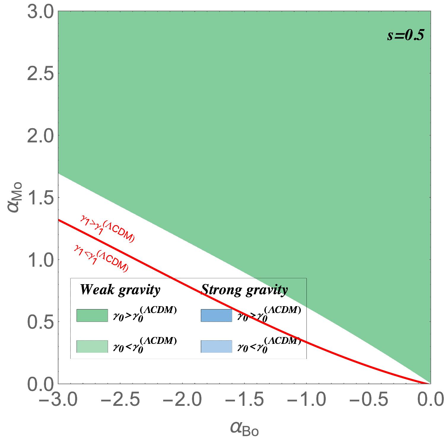
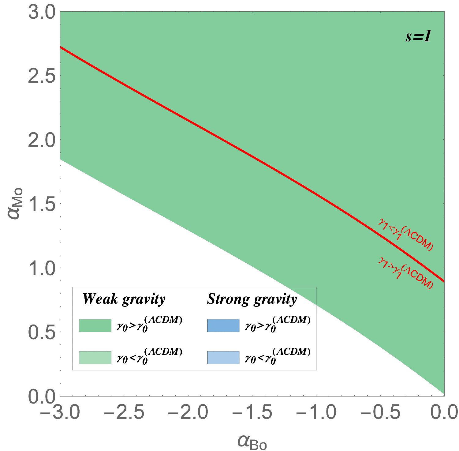
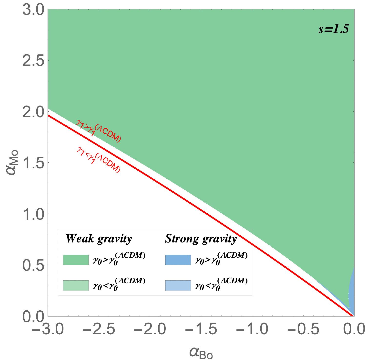
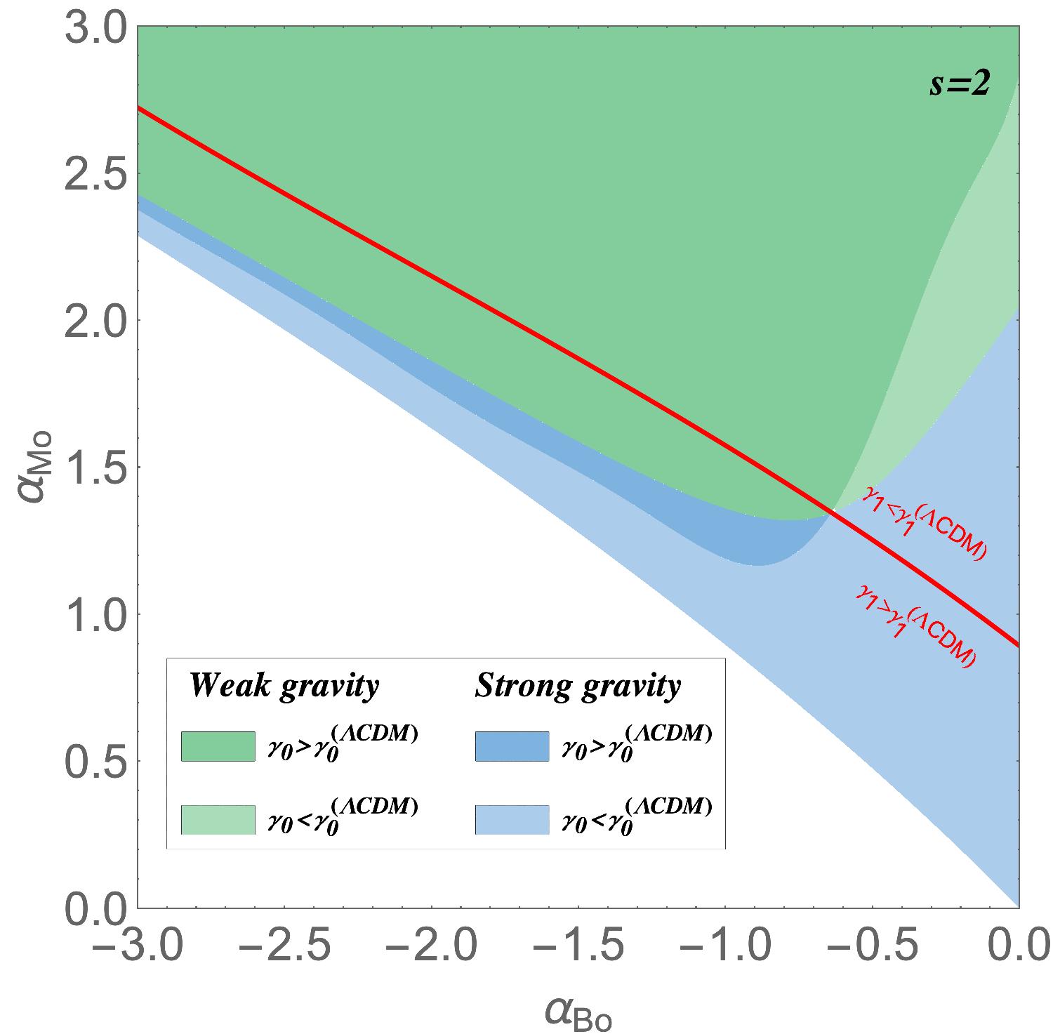
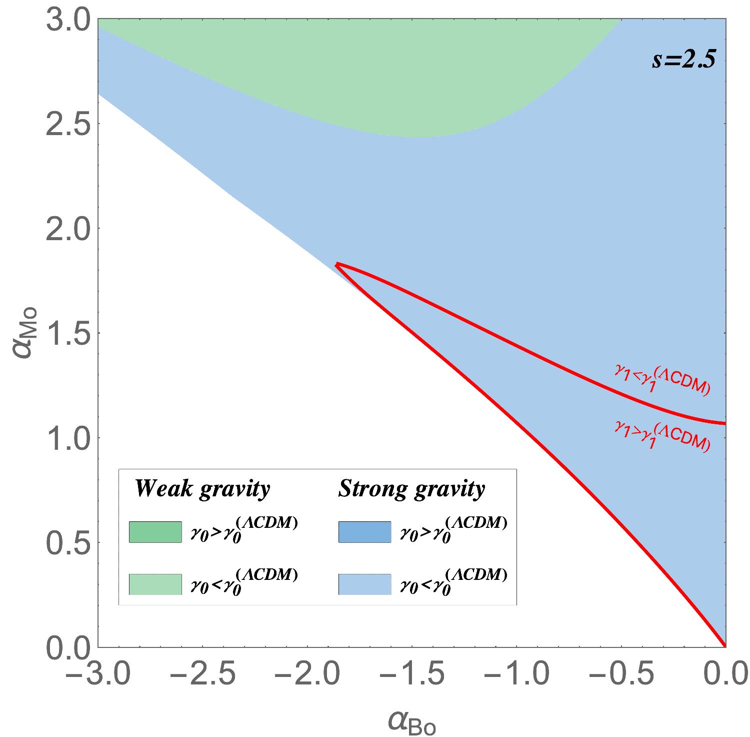
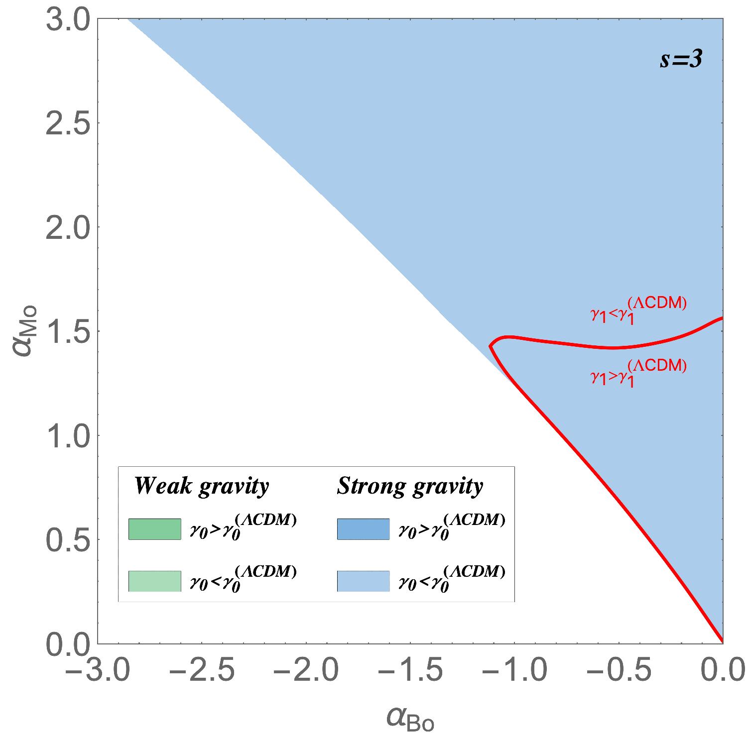
Figure 1: The stability (no ghost) region in the $\alpha_{M0}$-$\alpha_{B0}$ parameter space is shown and divided into a weak gravity regime today, $\mu_{0}\equiv\mu(z=0)<1$ (green area), and a strong gravity regime today, $\mu_{0}>1$ (blue area). This is obtained by demanding $c_{s}^{2}(z)>0$ at all times and assuming a flat $\Lambda$CDM background together with the parametrization Eq. (18) used here for the values $s=0.5,1,1.5,2,2.5,3$. The dark blue and dark green regions indicate $\gamma_{0}>\gamma_{0}^{\Lambda CDM}$, while the light blue and light green regions correspond to $\gamma_{0}<\gamma_{0}^{\Lambda CDM}$. Finally, the red curve determines the regions where either $\gamma_{1}>\gamma_{1}^{\Lambda CDM}$ or $\gamma_{1}<\gamma_{1}^{\Lambda CDM}$. We see in particular that for $s\leq 2$, essentially the weak gravity regime today is selected. In the light green region, $\mu$ crosses $1$ downwards with expansion, while it crosses upwards in the dark blue region.

For each region, we show in Fig. 1 the strong gravity regime today

$$\mu(z=0)>1~{},$$ (52)

and weak gravity regime today

$$\mu(z=0)<1~{}.$$ (53)

We can see that for small values of ($\alpha_{B0}$, $\alpha_{M0}$) and for small $s$, we have $\mu<1$ while for larger $s$ gravity is stronger. Gravity is weak today for $s<2$ and strong if $s>2$ for most of the parameters in the range $-3\leq\alpha_{B0}\leq 0$ and $0\leq\alpha_{M0}\leq 3$.

The growth rate of perturbations evolves according to the equation

$$\frac{df}{dx}+f^{2}+\frac{1}{2}\left(1-\frac{d\ln\Omega_{m}}{dx}\right)f=\frac{3}{2}\frac{G_{growth}}{G}\Omega_{m}~{}$$ (54)

where $x\equiv\ln a$. From Eq. (41) we have that the density perturbation $\delta_{m}$ is connected to the growth rate $f$ as

$$\delta_{m}(a)=\delta_{i}~{}{\rm exp}\left[\int_{x_{i}}^{x}f(x^{\prime})dx^{\prime}\right]~{}.$$ (55)

In the special case where the growing mode satisfies $\delta_{m}\propto a^{p}$, we have $f=p$ and thus $f\to 1$ in $\Lambda$CDM for large $z$ as long as the decaying mode is negligible Calderon et al. (2019). In a $\Lambda$CDM universe we have

$$f=\Omega_{m}^{\gamma(z)}~{},$$ (56)

with $\gamma_{0}\equiv\gamma(z=0)\approx\frac{6}{11}$, the latter corresponds to the exact value deep in the matter era and $\gamma_{0}$ is only slightly higher. In $\Lambda$CDM, $\gamma$ is monotonically increasing with the expansion Calderon et al. (2019). In general, the growth index is thus redshift dependent, a strictly constant $\gamma$ being excluded inside GR though it is often quasi-constant on redshifts between today till deep in the matter era Polarski et al. (2016). Using the above definitions, we have represented in the same figure, the values of the growth index today $\gamma_{0}$ and its derivative $\gamma_{1}\equiv\gamma^{\prime}(z=0)$, where $\gamma_{0}$, $\gamma_{1}$ are parameters to be fit to data.

The $\gamma_{0},\gamma_{1}$ values are complementary to the $\mu$ values and add information about the perturbations dynamics in the past. On Fig.(1), $s=2$, it is seen that the curve $\mu=1$ crosses the curve $\gamma_{0}=\gamma_{0}^{\Lambda CDM}$. As we have a fixed $\Lambda$CDM background, it follows from the evolution equation for $\gamma$ that we must have there $\gamma_{1}=\gamma_{1}^{\Lambda CDM}$ which is nicely exhibited on our Figure. Furthermore, for that specific point, the value of $\mu$ in the recent past satisfies $\mu\approx 1$ on those redshifts for which $\gamma\approx\gamma_{0}^{\Lambda CDM}+\gamma_{1}^{\Lambda CDM}(1-a)$.

Notice that when $\gamma_{0}=\gamma_{0}^{\Lambda CDM}$, we are in the weak gravity regime for $\gamma_{1}<\gamma_{1}^{\Lambda CDM}$ and in the strong gravity regime for $\gamma_{1}>\gamma_{1}^{\Lambda CDM}$. Also if we consider $\gamma_{1}=\gamma_{1}^{\Lambda CDM}$, we have $\gamma_{0}<\gamma_{0}^{\Lambda CDM}$ for strong gravity and $\gamma_{0}>\gamma_{0}^{\Lambda CDM}$ for weak gravity today. These results obtained for our parametrized Horndeski models are in accordance with the results obtained earlier (see Fig. 7 in Gannouji and Polarski (2018)) in a (gravity) model independent way.

Using the observational constraints from $f\sigma_{8}$ and $E_{G}$ data, we find that for larger values of $s$ ($s\gtrsim 2$) the best fit selects an area violating the stability conditions, and therefore these values of $s$ should be ignored. Therefore, assuming a $\Lambda$CDM background and these data, we find that $s\leq 2$ is allowed. This implies that our data select essentially a weak gravity regime today as we have noted earlier, see Fig.(1). Also, because we have $\Sigma\leq\mu$ from Eq.(37), we obtain $\Sigma_{0}\leq 1$, a result which we have confirmed numerically. Even for $s=2$ where a small regime of strong gravity remains, we still have always $\Sigma_{0}\leq 1$. Fig.(2) exhibits these results with the $1\sigma$ and $2\sigma$ contour plots for the combined data.

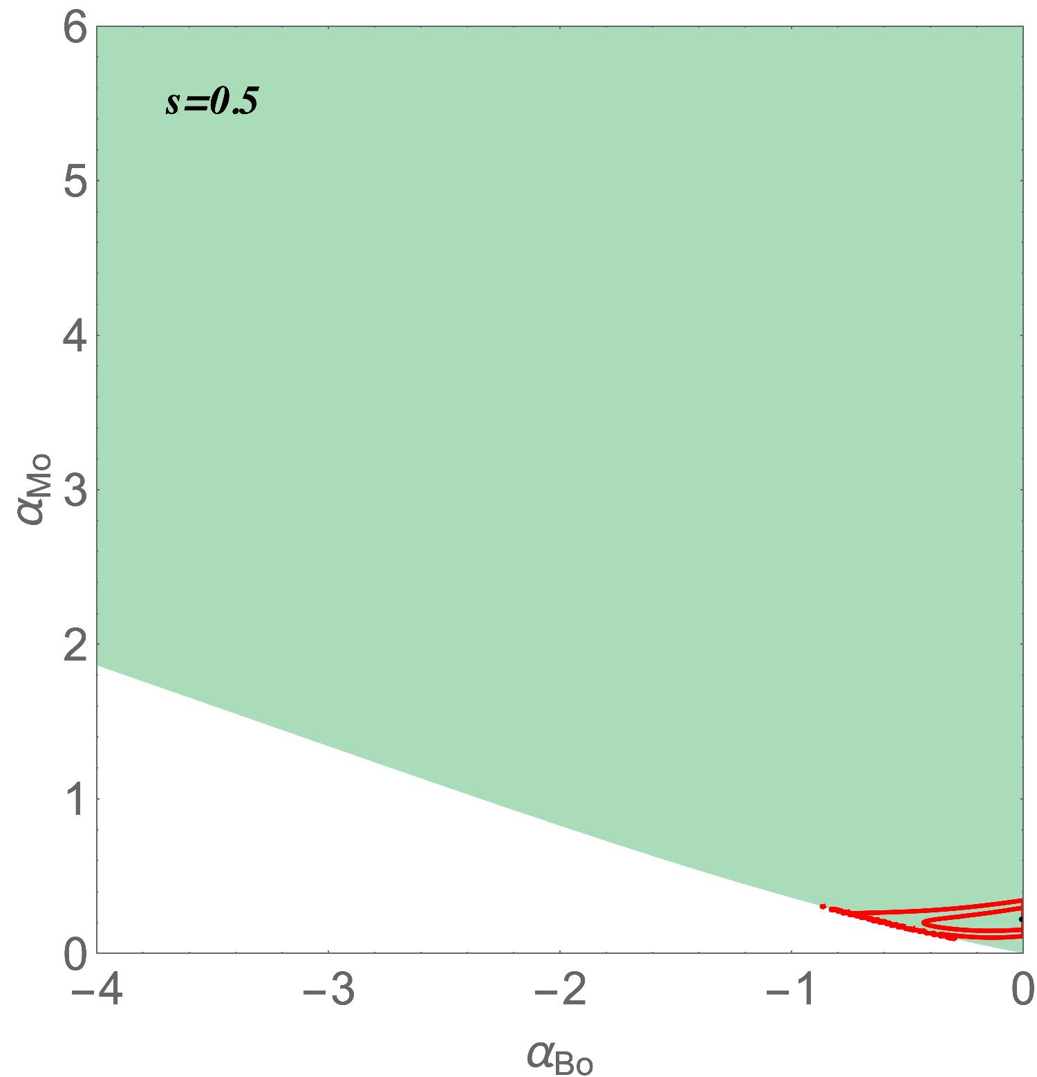
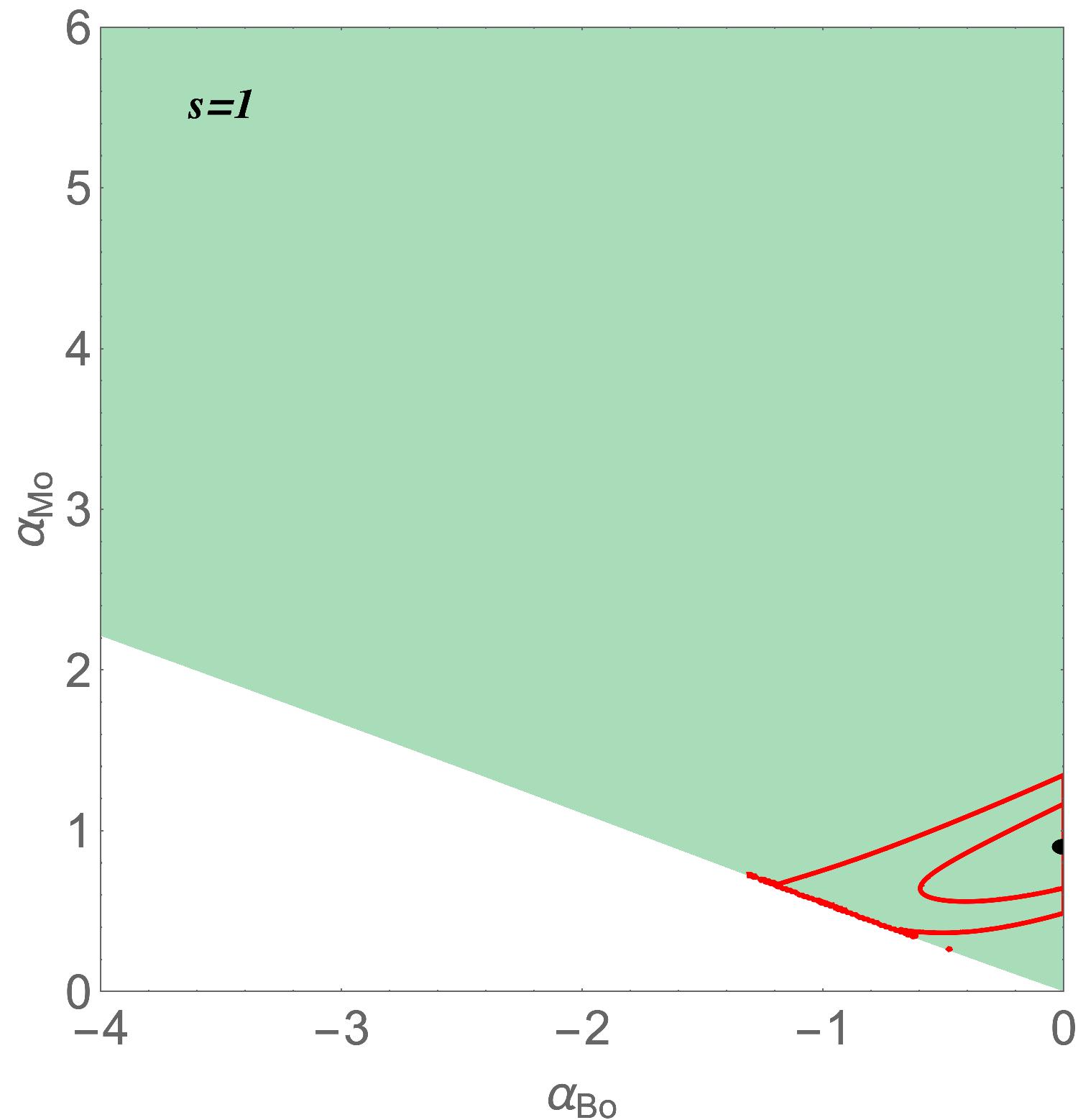
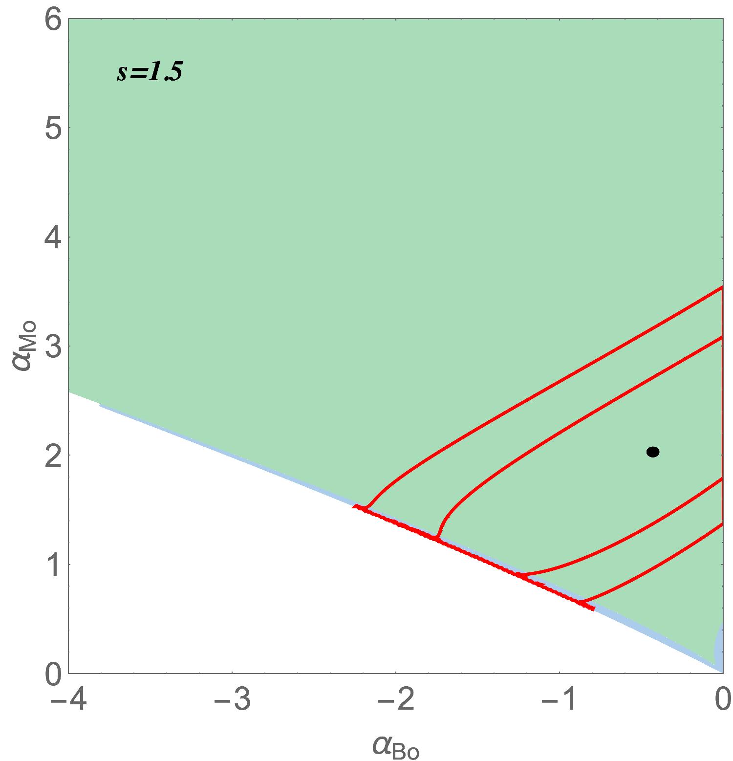
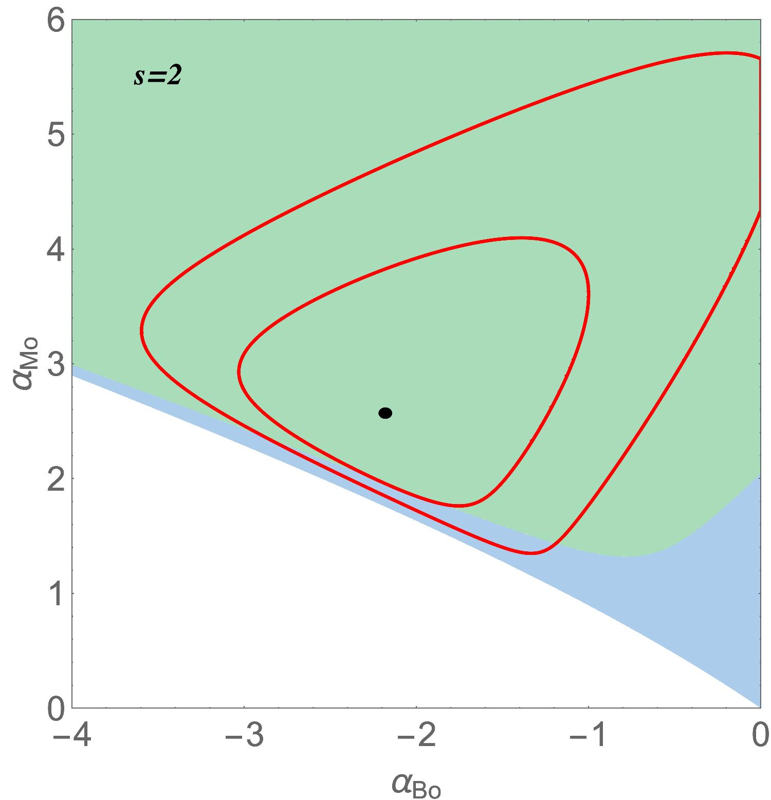
Figure 2: The best fit values of $\alpha_{B0}$ and $\alpha_{M0}$ are shown for $s=0.5,1,1.5,2$ using the combined constraints from the $f\sigma_{8}$ and $E_{G}$ data, $1\sigma$ and $2\sigma$ confidence regions are drawned (red curves). As in Fig.1, the green area corresponds to weak gravity today while the blue area represents strong gravity today. Observations give the constraint $\gamma_{0}>\gamma_{0}^{\Lambda CDM}$ for $s<2$, marginally allowing $\gamma_{0}<\gamma_{0}^{\Lambda CDM}$ for $s=2$. Note that for higher values of $s$, the best fit moves outside the colored region and is therefore ruled out.

V Conclusion - Outlook

Weak gravity is a difficult regime to be reached within viable modified gravity theories. We have shown that assuming a perfectly viable background solution, $\Lambda$CDM, we were able to constrain Horndeski models by using $f\sigma_{8}$ and $E_{G}$ data. Assuming only a power law parametrization for the parameters $(\alpha_{B},\alpha_{M})$, we found that viable models should verify the condition

$$\alpha_{B,0}<0~{}~{}~{}~{}~{}{\rm and}~{}~{}~{}~{}~{}\alpha_{M,0}>-\alpha_{B,0}/2$$ (57)

which constrain $G_{\text{lensing}}$ to be always smaller than $G_{\text{growth}}$.

Considering the $\Lambda$CDM background, we found that for $s<2$, most of the parameters $(\alpha_{B0},\alpha_{M0})$ produce weak gravity today while for $s>2$, we found $\mu_{0}>1$ for most of the parameters. The consideration of cosmological growth data favors $s\leq 2$, namely a mild evolution of the $\alpha_{i}$ parameters in the late universe, which in turn implies a weak gravity regime today and $\Sigma_{0}\leq 1$. We also found that for $s<2$, $\gamma_{0}>\gamma_{0}^{\Lambda CDM}$, while for $s>2$ we obtain $\gamma_{0}<\gamma_{0}^{\Lambda CDM}$. Therefore, data also select essentially $\gamma_{0}>\gamma_{0}^{\Lambda CDM}$ except for $s=2$ for which $\gamma_{0}<\gamma_{0}^{\Lambda CDM}$ is marginally allowed. Note that for $s=2$, in the region with $\mu_{0}<1$ and $\gamma_{0}<\gamma_{0}^{\Lambda CDM}$ (light green on Fig.1), gravity was strong in the near past ($z\lesssim 1)$, while in the region $\mu_{0}>1$ and $\gamma_{0}>\gamma_{0}^{\Lambda CDM}$ (dark blue on Fig.1), gravity was weak in the recent past. In some sense, the value of $\gamma_{0}$ indicates that gravity was either weak ($\gamma_{0}>\gamma_{0}^{\Lambda CDM}$ and $\mu_{0}>1$) or strong ($\gamma_{0}<\gamma_{0}^{\Lambda CDM}$ and $\mu_{0}<1$) when we average over the recent past, while $\mu_{0}$ determines the strength of gravity today. For example, in the light green region where $\mu_{0}<1$, the average of $\mu(z)$ over redshift $(0,1)$ is larger than 1. We encountered the same behavior in the dark blue region where gravity is strong today and weak on average for most part of the region. Therefore, the pairs $(\gamma_{0},\gamma_{1})$ add information on the past dynamics of $\mu$.

For models with $\gamma_{1}=\gamma_{1}^{\Lambda CDM}$, we have $\gamma_{0}<\gamma_{0}^{\Lambda CDM}$ when gravity is strong today and $\gamma_{0}>\gamma_{0}^{\Lambda CDM}$ when gravity is weak today. Also when $\gamma_{0}=\gamma_{0}^{\Lambda CDM}$, we have weak gravity when $\gamma_{1}>\gamma_{1}^{\Lambda CDM}$ while we have strong gravity when $\gamma_{1}<\gamma_{1}^{\Lambda CDM}$.

In summary, we have proved that under mild assumptions, we could have a consistent and viable weak gravity regime today. It is thus interesting to know how generic this result is. It is interesting that the model we have assumed is observationally incompatible at more than $2\sigma$ with $M_{*}=M_{p}$ today (at least for $s\gtrsim 0.5$). Hence the local value of $M_{*}$ must be necessarily different from its assumed value on cosmic scales today, eq.(20), and some screening mechanism must be at work in order to make the model viable. As we have mentioned earlier, this is a delicate issue. Even in the absence of screening, our results leave open the possibility to have viable models with $s<0.5$ satisfying $\alpha_{M0}\ll 2s$. Of course, in that case, $M_{*}$ would be (very) weakly varying at all times.

We plan to investigate in a future work the relevance, regarding the obtained results, of the two main assumptions made in this work, namely the power-law parametrization of the free functions $\alpha_{i}$ and the $\Lambda$CDM background expansion (for an alternative approach see e.g. Garcia-Quintero et al. (2020)). For example, in the case of minimal scalar-tensor theories, it has been shown that values of $w<-1$ can indeed lead to $\mu<1$ Gannouji et al. (2018); Kazantzidis and Perivolaropoulos (2019), while it is otherwise impossible to realize. Despite strong restrictions on Horndeski models coming from the gravitational waves speed, viable models could still provide interesting cosmological scenarios with varying gravitational couplings.

Appendix A Definitions

The background quantities $\mathcal{E}_{DE}$ and $\mathcal{P}_{DE}$ are defined as Bellini and Sawicki (2014)

$$\begin{split}\mathcal{E}_{DE}\equiv&-K+2X\left(K_{X}-G_{3\phi}\right)+6\dot{\phi}H\left(XG_{3X}-G_{4\phi}-2XG_{4\phi X}\right)+\\ &+12H^{2}X\left(G_{4X}+2XG_{4XX}-G_{5\phi}-XG_{5\phi X}\right)+4\dot{\phi}H^{3}X\left(G_{5X}+XG_{5XX}\right)\end{split}$$ (58)

$$\begin{split}\mathcal{P}_{DE}\equiv&K-2X\left(G_{3\phi}-2G_{4\phi\phi}\right)+4\dot{\phi}H\left(G_{4\phi}-2XG_{4\phi X}+XG_{5\phi\phi}\right)-\\ &-M_{*}^{2}\alpha_{B}H\frac{\ddot{\phi}}{\dot{\phi}}-4H^{2}X^{2}G_{5\phi X}+2\dot{\phi}H^{3}XG_{5X}\end{split}$$ (59)

Note that in the literature there appear various definitions of the energy density associated to the dark energy (see Amendola et al. (2020)). However we use here the effective DE energy density $\rho_{DE}$ and pressure $P_{DE}$ based on an Einsteinian representation of modified gravity Boisseau et al. (2000); Gannouji et al. (2006).

Appendix B DATA USED IN THE ANALYSIS

In this appendix we present the data used in the analysis.

Table 1: The $f\sigma_{8}$ updated data compilation of Ref. Skara and Perivolaropoulos (2020) used in the present analysis.

Index	Dataset	$z$	$f\sigma_{8}(z)$	Refs.	Year	Fiducial Cosmology
1	2MRS	0.02	$0.314\pm 0.048$	Davis et al. (2011), Hudson and Turnbull (2012)	13 November 2010	$(\Omega_{m},\Omega_{K},\sigma_{8})=(0.266,0,0.65)$
2	SDSS-LRG-200	$0.25$	$0.3512\pm 0.0583$	Samushia et al. (2012)	9 December 2011	$(\Omega_{m},\Omega_{K},\sigma_{8})=(0.276,0,0.8)$
3	WiggleZ	$0.44$	$0.413\pm 0.080$	Blake et al. (2012)	12 June 2012	$(\Omega_{m},h,\sigma_{8})=(0.27,0.71,0.8)$
4	WiggleZ	$0.60$	$0.390\pm 0.063$	Blake et al. (2012)	12 June 2012
5	WiggleZ	$0.73$	$0.437\pm 0.072$	Blake et al. (2012)	12 June 2012
6	GAMA	$0.18$	$0.360\pm 0.090$	Blake et al. (2013)	22 September 2013	$(\Omega_{m},\Omega_{K},\sigma_{8})=(0.27,0,0.8)$
7	SDSS-MGS	$0.15$	$0.490\pm 0.145$	Howlett et al. (2015)	30 January 2015	$(\Omega_{m},h,\sigma_{8})=(0.31,0.67,0.83)$
8	SDSS-veloc	$0.10$	$0.370\pm 0.130$	Feix et al. (2015)	16 June 2015	$(\Omega_{m},\Omega_{K},\sigma_{8}$)$=(0.3,0,0.89)$Tegmark:2003uf
9	FastSound	$1.40$	$0.482\pm 0.116$	Okumura et al. (2016)	25 November 2015	$(\Omega_{m},\Omega_{K},\sigma_{8}$)$=(0.27,0,0.82)$Hinshaw et al. (2013)
10	BOSS DR12	$0.38$	$0.497\pm 0.045$	Alam et al. (2017)	11 July 2016	$(\Omega_{m},\Omega_{K},\sigma_{8})=(0.31,0,0.8)$
11	BOSS DR12	$0.51$	$0.458\pm 0.038$	Alam et al. (2017)	11 July 2016
12	BOSS DR12	$0.61$	$0.436\pm 0.034$	Alam et al. (2017)	11 July 2016
13	VIPERS v7	$1.05$	$0.280\pm 0.080$	Wilson (2016)	26 October 2016
14	BOSS LOWZ	$0.32$	$0.427\pm 0.056$	Gil-Marín et al. (2017)	26 October 2016	$(\Omega_{m},\Omega_{K},\sigma_{8})=(0.31,0,0.8475)$
15	VIPERS	$0.727$	$0.296\pm 0.0765$	Hawken et al. (2017)	21 November 2016	$(\Omega_{m},\Omega_{K},\sigma_{8})=(0.31,0,0.7)$
16	6dFGS+SnIa	$0.02$	$0.428\pm 0.0465$	Huterer et al. (2017)	29 November 2016	$(\Omega_{m},h,\sigma_{8})=(0.3,0.683,0.8)$
17	2MTF	0.001	$0.505\pm 0.085$	Howlett et al. (2017)	16 June 2017	$(\Omega_{m},\sigma_{8})=(0.3121,0.815)$
18	BOSS DR12	$0.31$	$0.384\pm 0.083$	Wang et al. (2017)	15 September 2017	$(\Omega_{m},h,\sigma_{8})=(0.307,0.6777,0.8288)$
19	BOSS DR12	$0.36$	$0.409\pm 0.098$	Wang et al. (2017)	15 September 2017
20	BOSS DR12	$0.40$	$0.461\pm 0.086$	Wang et al. (2017)	15 September 2017
21	BOSS DR12	$0.44$	$0.426\pm 0.062$	Wang et al. (2017)	15 September 2017
22	BOSS DR12	$0.48$	$0.458\pm 0.063$	Wang et al. (2017)	15 September 2017
23	BOSS DR12	$0.52$	$0.483\pm 0.075$	Wang et al. (2017)	15 September 2017
24	BOSS DR12	$0.56$	$0.472\pm 0.063$	Wang et al. (2017)	15 September 2017
25	BOSS DR12	$0.59$	$0.452\pm 0.061$	Wang et al. (2017)	15 September 2017
26	BOSS DR12	$0.64$	$0.379\pm 0.054$	Wang et al. (2017)	15 September 2017
27	SDSS-IV	$0.978$	$0.379\pm 0.176$	Zhao et al. (2018)	9 January 2018	$(\Omega_{m},\sigma_{8})=(0.31,0.8)$
28	SDSS-IV	$1.23$	$0.385\pm 0.099$	Zhao et al. (2018)	9 January 2018
29	SDSS-IV	$1.526$	$0.342\pm 0.070$	Zhao et al. (2018)	9 January 2018
30	SDSS-IV	$1.944$	$0.364\pm 0.106$	Zhao et al. (2018)	9 January 2018
31	VIPERS PDR2	$0.60$	$0.49\pm 0.12$	Mohammad et al. (2018)	6 June 2018	$(\Omega_{b},\Omega_{m},h,\sigma_{8})=(0.045,0.31,0.7,0.8)$
32	VIPERS PDR2	$0.86$	$0.46\pm 0.09$	Mohammad et al. (2018)	6 June 2018
33	BOSS DR12 voids	$0.57$	$0.501\pm 0.051$	Nadathur et al. (2019)	1 April 2019	$(\Omega_{b},\Omega_{m},h,\sigma_{8})=(0.0482,0.307,0.6777,0.8228)$
34	2MTF 6dFGSv	$0.03$	$0.404\pm 0.0815$	Qin et al. (2019)	7 June 2019	$(\Omega_{b},\Omega_{m},h,\sigma_{8})=(0.0491,0.3121,0.6571,0.815)$
35	SDSS-IV	$0.72$	$0.454\pm 0.139$	Icaza-Lizaola et al. (2019)	17 September 2019	$(\Omega_{m},\Omega_{b}h^{2},\sigma_{8})=(0.31,0.022,0.8)$

Table 2: The $E_{G}(z)$ data compilation of Ref. Skara and Perivolaropoulos (2020) used in the present analysis.

Index	Dataset	$z$	$E_{G}(z)$	$\sigma_{E_{G}}$	Scale [Mpc/h]	Reference
1	KiDS GAMA	0.267	0.43	0.13	$5<R<40$	Amon et al. (2018)
2	KiDS 2dFLenS BOSS LOWZ 2dFLOZ	0.305	0.27	0.08	$5<R<60$	Amon et al. (2018)
3	RCSLenS CFHTLenS WiggleZ BOSS WGZLoZ LOWZ	0.32	0.40	0.09	$R>3$	Blake et al. (2016)
4	KiDS 2dFLenS BOSS CMASS 2dFHIZ	0.554	0.26	0.07	$5<R<60$	Amon et al. (2018)
5	RCSLenS CFHTLenS WiggleZ BOSS WGZHiZ CMASS	0.57	0.31	0.06	$R>3$	Blake et al. (2016)
6	RCSLenS CFHTLenS WiggleZ BOSS WGZHiZ CMASS	0.57	0.30	0.07	$R>10$	Blake et al. (2016)
7	CFHTLenS VIPERS	0.60	0.16	0.09	$3<R<20$	de la Torre et al. (2017)
8	CFHTLenS VIPERS	0.86	0.09	0.07	$3<R<20$	de la Torre et al. (2017)

References

- Addison et al. (2016) G.E. Addison, Y. Huang, D.J. Watts, C.L. Bennett, M. Halpern, G. Hinshaw, and J.L. Weiland, “Quantifying discordance in the 2015 Planck CMB spectrum,” Astrophys. J. 818, 132 (2016), arXiv:1511.00055 [astro-ph.CO] .
- Aghanim et al. (2019) N. Aghanim et al. (Planck), “Planck 2018 results. V. CMB power spectra and likelihoods,” (2019), arXiv:1907.12875 [astro-ph.CO] .
- Addison et al. (2018) G.E. Addison, D.J. Watts, C.L. Bennett, M. Halpern, G. Hinshaw, and J.L. Weiland, “Elucidating CDM: Impact of Baryon Acoustic Oscillation Measurements on the Hubble Constant Discrepancy,” Astrophys. J. 853, 119 (2018), arXiv:1707.06547 [astro-ph.CO] .
- Bernui et al. (2018) Armando Bernui, Camila P. Novaes, Thiago S. Pereira, and Glenn D. Starkman, “Topology and the suppression of CMB large-angle correlations,” (2018), arXiv:1809.05924 [astro-ph.CO] .
- Schwarz et al. (2016) Dominik J. Schwarz, Craig J. Copi, Dragan Huterer, and Glenn D. Starkman, “CMB Anomalies after Planck,” Class. Quant. Grav. 33, 184001 (2016), arXiv:1510.07929 [astro-ph.CO] .
- Bullock and Boylan-Kolchin (2017) James S. Bullock and Michael Boylan-Kolchin, “Small-Scale Challenges to the CDM Paradigm,” Ann. Rev. Astron. Astrophys. 55, 343–387 (2017), arXiv:1707.04256 [astro-ph.CO] .
- Ade et al. (2016) P. A. R. Ade et al. (Planck), “Planck 2015 results. XIII. Cosmological parameters,” Astron. Astrophys. 594, A13 (2016), arXiv:1502.01589 [astro-ph.CO] .
- Aghanim et al. (2018) N. Aghanim et al. (Planck), “Planck 2018 results. VI. Cosmological parameters,” (2018), arXiv:1807.06209 [astro-ph.CO] .
- Riess et al. (2016) Adam G. Riess et al., “A 2.4% Determination of the Local Value of the Hubble Constant,” Astrophys. J. 826, 56 (2016), arXiv:1604.01424 [astro-ph.CO] .
- Riess et al. (2018) Adam G. Riess et al., “Milky Way Cepheid Standards for Measuring Cosmic Distances and Application to Gaia DR2: Implications for the Hubble Constant,” Astrophys. J. 861, 126 (2018), arXiv:1804.10655 [astro-ph.CO] .
- Birrer et al. (2019) S. Birrer et al., “H0LiCOW - IX. Cosmographic analysis of the doubly imaged quasar SDSS 1206+4332 and a new measurement of the Hubble constant,” Mon. Not. Roy. Astron. Soc. 484, 4726 (2019), arXiv:1809.01274 [astro-ph.CO] .
- Horndeski (1974) Gregory Walter Horndeski, “Second-order scalar-tensor field equations in a four-dimensional space,” Int. J. Theor. Phys. 10, 363–384 (1974).
- Deffayet et al. (2011) C. Deffayet, Xian Gao, D. A. Steer, and G. Zahariade, “From k-essence to generalised Galileons,” Phys. Rev. D84, 064039 (2011), arXiv:1103.3260 [hep-th] .
- Kase and Tsujikawa (2019) Ryotaro Kase and Shinji Tsujikawa, “Dark energy in Horndeski theories after GW170817: A review,” Int. J. Mod. Phys. D 28, 1942005 (2019), arXiv:1809.08735 [gr-qc] .
- Kobayashi (2019) Tsutomu Kobayashi, “Horndeski theory and beyond: a review,” Rept. Prog. Phys. 82, 086901 (2019), arXiv:1901.07183 [gr-qc] .
- Ostrogradsky (1850) M. Ostrogradsky, “Mémoires sur les équations différentielles, relatives au problème des isopérimètres,” Mem. Acad. St. Petersbourg 6, 385–517 (1850).
- Woodard (2015) Richard P. Woodard, “Ostrogradsky’s theorem on Hamiltonian instability,” Scholarpedia 10, 32243 (2015), arXiv:1506.02210 [hep-th] .
- De Felice and Tsujikawa (2010a) Antonio De Felice and Shinji Tsujikawa, “f(R) theories,” Living Rev. Rel. 13, 3 (2010a), arXiv:1002.4928 [gr-qc] .
- Brans and Dicke (1961) C. Brans and R. H. Dicke, “Mach’s principle and a relativistic theory of gravitation,” Phys. Rev. 124, 925–935 (1961).
- De Felice and Tsujikawa (2010b) Antonio De Felice and Shinji Tsujikawa, “Generalized Brans-Dicke theories,” JCAP 07, 024 (2010b), arXiv:1005.0868 [astro-ph.CO] .
- Abbott et al. (2017a) B. P. Abbott et al. (LIGO Scientific, Virgo), “GW170817: Observation of Gravitational Waves from a Binary Neutron Star Inspiral,” Phys. Rev. Lett. 119, 161101 (2017a), arXiv:1710.05832 [gr-qc] .
- Goldstein et al. (2017) A. Goldstein et al., “An Ordinary Short Gamma-Ray Burst with Extraordinary Implications: Fermi-GBM Detection of GRB 170817A,” Astrophys. J. 848, L14 (2017), arXiv:1710.05446 [astro-ph.HE] .
- de Rham and Melville (2018) Claudia de Rham and Scott Melville, “Gravitational Rainbows: LIGO and Dark Energy at its Cutoff,” Phys. Rev. Lett. 121, 221101 (2018), arXiv:1806.09417 [hep-th] .
- Bellini and Sawicki (2014) Emilio Bellini and Ignacy Sawicki, “Maximal freedom at minimum cost: linear large-scale structure in general modifications of gravity,” JCAP 1407, 050 (2014), arXiv:1404.3713 [astro-ph.CO] .
- Sbisà (2015) Fulvio Sbisà, “Classical and quantum ghosts,” Eur. J. Phys. 36, 015009 (2015), arXiv:1406.4550 [hep-th] .
- Denissenya and Linder (2018) Mikhail Denissenya and Eric V. Linder, “Gravity’s Islands: Parametrizing Horndeski Stability,” JCAP 1811, 010 (2018), arXiv:1808.00013 [astro-ph.CO] .
- De Felice et al. (2011) Antonio De Felice, Tsutomu Kobayashi, and Shinji Tsujikawa, “Effective gravitational couplings for cosmological perturbations in the most general scalar-tensor theories with second-order field equations,” Phys. Lett. B706, 123–133 (2011), arXiv:1108.4242 [gr-qc] .
- Sawicki and Bellini (2015) Ignacy Sawicki and Emilio Bellini, “Limits of quasistatic approximation in modified-gravity cosmologies,” Phys. Rev. D92, 084061 (2015), arXiv:1503.06831 [astro-ph.CO] .
- Boisseau et al. (2000) B. Boisseau, Gilles Esposito-Farese, D. Polarski, and Alexei A. Starobinsky, “Reconstruction of a scalar tensor theory of gravity in an accelerating universe,” Phys. Rev. Lett. 85, 2236 (2000), arXiv:gr-qc/0001066 [gr-qc] .
- Esposito-Farese and Polarski (2001) Gilles Esposito-Farese and D. Polarski, “Scalar tensor gravity in an accelerating universe,” Phys. Rev. D63, 063504 (2001), arXiv:gr-qc/0009034 [gr-qc] .
- Espejo et al. (2019) Juan Espejo, Simone Peirone, Marco Raveri, Kazuya Koyama, Levon Pogosian, and Alessandra Silvestri, “Phenomenology of Large Scale Structure in scalar-tensor theories: joint prior covariance of , and in Horndeski,” Phys. Rev. D 99, 023512 (2019), arXiv:1809.01121 [astro-ph.CO] .
- Pace et al. (2019) Francesco Pace, Richard A. Battye, Boris Bolliet, and Damien Trinh, “Dark sector evolution in Horndeski models,” JCAP 09, 018 (2019), arXiv:1905.06795 [astro-ph.CO] .
- Kobayashi et al. (2011) Tsutomu Kobayashi, Masahide Yamaguchi, and Jun’ichi Yokoyama, “Generalized G-inflation: Inflation with the most general second-order field equations,” Prog. Theor. Phys. 126, 511–529 (2011), arXiv:1105.5723 [hep-th] .
- Ishak et al. (2019) Mustapha Ishak et al., “Modified Gravity and Dark Energy models Beyond CDM Testable by LSST,” (2019), arXiv:1905.09687 [astro-ph.CO] .
- Gleyzes et al. (2015) Jérôme Gleyzes, David Langlois, and Filippo Vernizzi, “A unifying description of dark energy,” Int. J. Mod. Phys. D23, 1443010 (2015), arXiv:1411.3712 [hep-th] .
- Savchenko et al. (2017) V. Savchenko et al., “INTEGRAL Detection of the First Prompt Gamma-Ray Signal Coincident with the Gravitational-wave Event GW170817,” Astrophys. J. 848, L15 (2017), arXiv:1710.05449 [astro-ph.HE] .
- Abbott et al. (2017b) B. P. Abbott et al. (LIGO Scientific, Virgo, Fermi-GBM, INTEGRAL), “Gravitational Waves and Gamma-rays from a Binary Neutron Star Merger: GW170817 and GRB 170817A,” Astrophys. J. 848, L13 (2017b), arXiv:1710.05834 [astro-ph.HE] .
- Kennedy et al. (2018) Joe Kennedy, Lucas Lombriser, and Andy Taylor, “Reconstructing Horndeski theories from phenomenological modified gravity and dark energy models on cosmological scales,” Phys. Rev. D98, 044051 (2018), arXiv:1804.04582 [astro-ph.CO] .
- Tsujikawa (2007) Shinji Tsujikawa, “Matter density perturbations and effective gravitational constant in modified gravity models of dark energy,” Phys. Rev. D76, 023514 (2007), arXiv:0705.1032 [astro-ph] .
- Saltas et al. (2014) Ippocratis D. Saltas, Ignacy Sawicki, Luca Amendola, and Martin Kunz, “Anisotropic Stress as a Signature of Nonstandard Propagation of Gravitational Waves,” Phys. Rev. Lett. 113, 191101 (2014), arXiv:1406.7139 [astro-ph.CO] .
- Linder (2018) Eric V. Linder, “No Slip Gravity,” JCAP 1803, 005 (2018), arXiv:1801.01503 [astro-ph.CO] .
- Reischke et al. (2019) Robert Reischke, Alessio Spurio Mancini, Björn Malte Schäfer, and Philipp M. Merkel, “Investigating scalar–tensor gravity with statistics of the cosmic large-scale structure,” Mon. Not. Roy. Astron. Soc. 482, 3274–3287 (2019), arXiv:1804.02441 [astro-ph.CO] .
- Amendola et al. (2020) Luca Amendola, Dario Bettoni, Ana Marta Pinho, and Santiago Casas, “Measuring gravity at cosmological scales,” Universe 6, 20 (2020), arXiv:1902.06978 [astro-ph.CO] .
- Gannouji et al. (2006) Radouane Gannouji, David Polarski, Andre Ranquet, and Alexei A. Starobinsky, “Scalar-Tensor Models of Normal and Phantom Dark Energy,” JCAP 0609, 016 (2006), arXiv:astro-ph/0606287 [astro-ph] .
- Nesseris et al. (2017) Savvas Nesseris, George Pantazis, and Leandros Perivolaropoulos, “Tension and constraints on modified gravity parametrizations of from growth rate and Planck data,” Phys. Rev. D96, 023542 (2017), arXiv:1703.10538 [astro-ph.CO] .
- De Felice et al. (2012) Antonio De Felice, Ryotaro Kase, and Shinji Tsujikawa, “Vainshtein mechanism in second-order scalar-tensor theories,” Phys. Rev. D 85, 044059 (2012), arXiv:1111.5090 [gr-qc] .
- Babichev et al. (2011) Eugeny Babichev, Cedric Deffayet, and Gilles Esposito-Farese, “Constraints on Shift-Symmetric Scalar-Tensor Theories with a Vainshtein Mechanism from Bounds on the Time Variation of G,” Phys. Rev. Lett. 107, 251102 (2011), arXiv:1107.1569 [gr-qc] .
- Kimura et al. (2012) Rampei Kimura, Tsutomu Kobayashi, and Kazuhiro Yamamoto, “Vainshtein screening in a cosmological background in the most general second-order scalar-tensor theory,” Phys. Rev. D 85, 024023 (2012), arXiv:1111.6749 [astro-ph.CO] .
- Williams et al. (2004) James G. Williams, Slava G. Turyshev, and Dale H. Boggs, “Progress in lunar laser ranging tests of relativistic gravity,” Phys. Rev. Lett. 93, 261101 (2004), arXiv:gr-qc/0411113 .
- Dar et al. (2019) Furqan Dar, Claudia De Rham, J. Tate Deskins, John T. Giblin, and Andrew J. Tolley, “Scalar Gravitational Radiation from Binaries: Vainshtein Mechanism in Time-dependent Systems,” Class. Quant. Grav. 36, 025008 (2019), arXiv:1808.02165 [hep-th] .
- Macaulay et al. (2013) Edward Macaulay, Ingunn Kathrine Wehus, and Hans Kristian Eriksen, “Lower Growth Rate from Recent Redshift Space Distortion Measurements than Expected from Planck,” Phys. Rev. Lett. 111, 161301 (2013), arXiv:1303.6583 [astro-ph.CO] .
- Johnson et al. (2016) Andrew Johnson, Chris Blake, Jason Dossett, Jun Koda, David Parkinson, and Shahab Joudaki, “Searching for Modified Gravity: Scale and Redshift Dependent Constraints from Galaxy Peculiar Velocities,” Mon. Not. Roy. Astron. Soc. 458, 2725–2744 (2016), arXiv:1504.06885 [astro-ph.CO] .
- Tsujikawa (2015) Shinji Tsujikawa, “Possibility of realizing weak gravity in redshift space distortion measurements,” Phys. Rev. D92, 044029 (2015), arXiv:1505.02459 [astro-ph.CO] .
- Solà (2016) Joan Solà, “Cosmological constant vis-a-vis dynamical vacuum: bold challenging the CDM,” Int. J. Mod. Phys. A31, 1630035 (2016), arXiv:1612.02449 [astro-ph.CO] .
- Wang et al. (2016) B. Wang, E. Abdalla, F. Atrio-Barandela, and D. Pavon, “Dark Matter and Dark Energy Interactions: Theoretical Challenges, Cosmological Implications and Observational Signatures,” Rept. Prog. Phys. 79, 096901 (2016), arXiv:1603.08299 [astro-ph.CO] .
- Basilakos and Nesseris (2017) Spyros Basilakos and Savvas Nesseris, “Conjoined constraints on modified gravity from the expansion history and cosmic growth,” Phys. Rev. D96, 063517 (2017), arXiv:1705.08797 [astro-ph.CO] .
- Kazantzidis and Perivolaropoulos (2018) Lavrentios Kazantzidis and Leandros Perivolaropoulos, “Evolution of the tension with the Planck15/CDM determination and implications for modified gravity theories,” Phys. Rev. D97, 103503 (2018), arXiv:1803.01337 [astro-ph.CO] .
- Kazantzidis and Perivolaropoulos (2019) Lavrentios Kazantzidis and Leandros Perivolaropoulos, “Is gravity getting weaker at low z? Observational evidence and theoretical implications,” (2019), arXiv:1907.03176 [astro-ph.CO] .
- Skara and Perivolaropoulos (2020) F. Skara and L. Perivolaropoulos, “Tension of the statistic and redshift space distortion data with the Planck - model and implications for weakening gravity,” Phys. Rev. D101, 063521 (2020), arXiv:1911.10609 [astro-ph.CO] .
- Joudaki et al. (2017) Shahab Joudaki et al., “KiDS-450 + 2dFLenS: Cosmological parameter constraints from weak gravitational lensing tomography and overlapping redshift-space galaxy clustering,” (2017), 10.1093/mnras/stx2820, arXiv:1707.06627 [astro-ph.CO] .
- Amon et al. (2018) A. Amon et al., “KiDS+2dFLenS+GAMA: Testing the cosmological model with the statistic,” Mon. Not. Roy. Astron. Soc. 479, 3422–3437 (2018), arXiv:1711.10999 [astro-ph.CO] .
- Leonard et al. (2015) C. Danielle Leonard, Pedro G. Ferreira, and Catherine Heymans, “Testing gravity with : mapping theory onto observations,” JCAP 12, 051 (2015), arXiv:1510.04287 [astro-ph.CO] .
- Amendola et al. (2013) Luca Amendola, Martin Kunz, Mariele Motta, Ippocratis D. Saltas, and Ignacy Sawicki, “Observables and unobservables in dark energy cosmologies,” Phys. Rev. D87, 023501 (2013), arXiv:1210.0439 [astro-ph.CO] .
- Motta et al. (2013) Mariele Motta, Ignacy Sawicki, Ippocratis D. Saltas, Luca Amendola, and Martin Kunz, “Probing Dark Energy through Scale Dependence,” Phys. Rev. D88, 124035 (2013), arXiv:1305.0008 [astro-ph.CO] .
- Pinho et al. (2018) Ana Marta Pinho, Santiago Casas, and Luca Amendola, “Model-independent reconstruction of the linear anisotropic stress ,” JCAP 1811, 027 (2018), arXiv:1805.00027 [astro-ph.CO] .
- Verde (2010) L. Verde, “Statistical methods in cosmology,” Lecture Notes in Physics , 147–177 (2010).
- Alam et al. (2017) Shadab Alam et al. (BOSS), “The clustering of galaxies in the completed SDSS-III Baryon Oscillation Spectroscopic Survey: cosmological analysis of the DR12 galaxy sample,” Mon. Not. Roy. Astron. Soc. 470, 2617–2652 (2017), arXiv:1607.03155 [astro-ph.CO] .
- Scolnic et al. (2018) D. M. Scolnic et al., “The Complete Light-curve Sample of Spectroscopically Confirmed SNe Ia from Pan-STARRS1 and Cosmological Constraints from the Combined Pantheon Sample,” Astrophys. J. 859, 101 (2018), arXiv:1710.00845 [astro-ph.CO] .
- Calderon et al. (2019) R. Calderon, D. Felbacq, R. Gannouji, D. Polarski, and A. A. Starobinsky, “Global properties of the growth index of matter inhomogeneities in the universe,” Phys. Rev. D100, 083503 (2019), arXiv:1908.00117 [astro-ph.CO] .
- Polarski et al. (2016) David Polarski, Alexei A. Starobinsky, and Hector Giacomini, “When is the growth index constant?” JCAP 1612, 037 (2016), arXiv:1610.00363 [astro-ph.CO] .
- Gannouji and Polarski (2018) Radouane Gannouji and David Polarski, “Consistency of the expansion of the Universe with density perturbations,” Phys. Rev. D 98, 083533 (2018), arXiv:1805.08230 [astro-ph.CO] .
- Garcia-Quintero et al. (2020) Cristhian Garcia-Quintero, Mustapha Ishak, and Orion Ning, “Current constraints on deviations from General Relativity using binning in redshift and scale,” (2020), arXiv:2010.12519 [astro-ph.CO] .
- Gannouji et al. (2018) Radouane Gannouji, Lavrentios Kazantzidis, Leandros Perivolaropoulos, and David Polarski, “Consistency of modified gravity with a decreasing in a CDM background,” Phys. Rev. D98, 104044 (2018), arXiv:1809.07034 [gr-qc] .
- Davis et al. (2011) Marc Davis, Adi Nusser, Karen Masters, Christopher Springob, John P. Huchra, and Gerard Lemson, “Local Gravity versus Local Velocity: Solutions for and nonlinear bias,” Mon. Not. Roy. Astron. Soc. 413, 2906 (2011), arXiv:1011.3114 [astro-ph.CO] .
- Hudson and Turnbull (2012) Michael J. Hudson and Stephen J. Turnbull, “The growth rate of cosmic structure from peculiar velocities at low and high redshifts,” The Astrophysical Journal Letters 751, L30 (2012).
- Samushia et al. (2012) L. Samushia, W. J. Percival, and A. Raccanelli, “Interpreting large-scale redshift-space distortion measurements,” Monthly Notices of the Royal Astronomical Society 420, 2102–2119 (2012).
- Blake et al. (2012) C. Blake, S. Brough, M. Colless, C. Contreras, W. Couch, S. Croom, D. Croton, T. M. Davis, M. J. Drinkwater, K. Forster, D. Gilbank, M. Gladders, K. Glazebrook, B. Jelliffe, R. J. Jurek, I.-h. Li, B. Madore, D. C. Martin, K. Pimbblet, G. B. Poole, M. Pracy, R. Sharp, E. Wisnioski, D. Woods, T. K. Wyder, and H. K. C. Yee, “The WiggleZ Dark Energy Survey: joint measurements of the expansion and growth history at ,” mnras 425, 405–414 (2012), arXiv:1204.3674 .
- Blake et al. (2013) Chris Blake et al., “Galaxy And Mass Assembly (GAMA): improved cosmic growth measurements using multiple tracers of large-scale structure,” Mon. Not. Roy. Astron. Soc. 436, 3089 (2013), arXiv:1309.5556 [astro-ph.CO] .
- Howlett et al. (2015) Cullan Howlett, Ashley Ross, Lado Samushia, Will Percival, and Marc Manera, “The clustering of the SDSS main galaxy sample – II. Mock galaxy catalogues and a measurement of the growth of structure from redshift space distortions at ,” Mon. Not. Roy. Astron. Soc. 449, 848–866 (2015), arXiv:1409.3238 [astro-ph.CO] .
- Feix et al. (2015) Martin Feix, Adi Nusser, and Enzo Branchini, “Growth Rate of Cosmological Perturbations at from a New Observational Test,” Phys. Rev. Lett. 115, 011301 (2015), arXiv:1503.05945 [astro-ph.CO] .
- Okumura et al. (2016) Teppei Okumura et al., “The Subaru FMOS galaxy redshift survey (FastSound). IV. New constraint on gravity theory from redshift space distortions at ,” Publ. Astron. Soc. Jap. 68, 24 (2016), arXiv:1511.08083 [astro-ph.CO] .
- Hinshaw et al. (2013) G. Hinshaw et al. (WMAP), “Nine-Year Wilkinson Microwave Anisotropy Probe (WMAP) Observations: Cosmological Parameter Results,” Astrophys. J. Suppl. 208, 19 (2013), arXiv:1212.5226 [astro-ph.CO] .
- Wilson (2016) Michael J. Wilson, Geometric and growth rate tests of General Relativity with recovered linear cosmological perturbations, Ph.D. thesis, Edinburgh U. (2016), arXiv:1610.08362 [astro-ph.CO] .
- Gil-Marín et al. (2017) Héctor Gil-Marín, Will J. Percival, Licia Verde, Joel R. Brownstein, Chia-Hsun Chuang, Francisco-Shu Kitaura, Sergio A. Rodríguez-Torres, and Matthew D. Olmstead, “The clustering of galaxies in the SDSS-III Baryon Oscillation Spectroscopic Survey: RSD measurement from the power spectrum and bispectrum of the DR12 BOSS galaxies,” Mon. Not. Roy. Astron. Soc. 465, 1757–1788 (2017), arXiv:1606.00439 [astro-ph.CO] .
- Hawken et al. (2017) A. J. Hawken et al., “The VIMOS Public Extragalactic Redshift Survey: Measuring the growth rate of structure around cosmic voids,” Astron. Astrophys. 607, A54 (2017), arXiv:1611.07046 [astro-ph.CO] .
- Huterer et al. (2017) Dragan Huterer, Daniel Shafer, Daniel Scolnic, and Fabian Schmidt, “Testing CDM at the lowest redshifts with SN Ia and galaxy velocities,” JCAP 1705, 015 (2017), arXiv:1611.09862 [astro-ph.CO] .
- Howlett et al. (2017) Cullan Howlett, Lister Staveley-Smith, Pascal J. Elahi, Tao Hong, Tom H. Jarrett, D. Heath Jones, Bärbel S. Koribalski, Lucas M. Macri, Karen L. Masters, and Christopher M. Springob, “2MTF VI. Measuring the velocity power spectrum,” Mon. Not. Roy. Astron. Soc. 471, 3135 (2017), arXiv:1706.05130 [astro-ph.CO] .
- Wang et al. (2017) Yuting Wang, Gong-Bo Zhao, Chia-Hsun Chuang, Marcos Pellejero-Ibanez, Cheng Zhao, Francisco-Shu Kitaura, and Sergio Rodriguez-Torres, “The clustering of galaxies in the completed SDSS-III Baryon Oscillation Spectroscopic Survey: a tomographic analysis of structure growth and expansion rate from anisotropic galaxy clustering,” (2017), arXiv:1709.05173 [astro-ph.CO] .
- Zhao et al. (2018) Gong-Bo Zhao et al., “The clustering of the SDSS-IV extended Baryon Oscillation Spectroscopic Survey DR14 quasar sample: a tomographic measurement of cosmic structure growth and expansion rate based on optimal redshift weights,” (2018), arXiv:1801.03043 [astro-ph.CO] .
- Mohammad et al. (2018) F. G. Mohammad et al., “The VIMOS Public Extragalactic Redshift Survey (VIPERS): Unbiased clustering estimate with VIPERS slit assignment,” Astron. Astrophys. 619, A17 (2018), arXiv:1807.05999 [astro-ph.CO] .
- Nadathur et al. (2019) Seshadri Nadathur, Paul M. Carter, Will J. Percival, Hans A. Winther, and Julian Bautista, “Beyond BAO: Improving cosmological constraints from BOSS data with measurement of the void-galaxy cross-correlation,” Phys. Rev. D100, 023504 (2019), arXiv:1904.01030 [astro-ph.CO] .
- Qin et al. (2019) Fei Qin, Cullan Howlett, and Lister Staveley-Smith, “The redshift-space momentum power spectrum – II. Measuring the growth rate from the combined 2MTF and 6dFGSv surveys,” Mon. Not. Roy. Astron. Soc. 487, 5235–5247 (2019), arXiv:1906.02874 [astro-ph.CO] .
- Icaza-Lizaola et al. (2019) M. Icaza-Lizaola et al., “The clustering of the SDSS-IV extended Baryon Oscillation Spectroscopic Survey DR14 LRG sample: structure growth rate measurement from the anisotropic LRG correlation function in the redshift range 0.6 z 1.0,” (2019), arXiv:1909.07742 [astro-ph.CO] .
- Blake et al. (2016) Chris Blake et al., “RCSLenS: Testing gravitational physics through the cross-correlation of weak lensing and large-scale structure,” Mon. Not. Roy. Astron. Soc. 456, 2806–2828 (2016), arXiv:1507.03086 [astro-ph.CO] .
- de la Torre et al. (2017) S. de la Torre et al., “The VIMOS Public Extragalactic Redshift Survey (VIPERS). Gravity test from the combination of redshift-space distortions and galaxy-galaxy lensing at ,” Astron. Astrophys. 608, A44 (2017), arXiv:1612.05647 [astro-ph.CO] .