Decoupled Structure-Preserving Doubling Algorithm with Truncation for Large-Scale Algebraic Riccati Equations

Abstract

In [15] we propose a decoupled form of the structure-preserving doubling algorithm (dSDA). The method decouples the original two to four coupled recursions, enabling it to solve large-scale algebraic Riccati equations and other related problems. In this paper, we consider the numerical computations of the novel dSDA for solving large-scale continuous-time algebraic Riccati equations with low-rank structures (thus possessing numerically low-rank solutions). With the help of a new truncation strategy, the rank of the approximate solution is controlled. Consequently, large-scale problems can be treated efficiently. Illustrative numerical examples are presented to demonstrate and confirm our claims.

15A24, 65F30, 65H10

1 Introduction

A continuous-time algebraic Riccati equation (CARE) has the form:

(1) $$A^{\operatorname{\sf T}}X+XA-XGX+H=0,$$

where $A\in\mathbb{R}^{n\times n}$, $G=BR^{-1}B^{\operatorname{\sf T}}$ with $B\in\mathbb{R}^{n\times m}$ and $R>0$, and $H=C^{\operatorname{\sf T}}C\geq 0$ with $C\in\mathbb{R}^{l\times n}$. Here, a symmetric matrix $M>0$ ($\geq 0$) when all its eigenvalues are positive (non-negative). These algebraic Riccati equations arise in many classical applications such as model reduction, filtering and control theory; please refer to [9, 10, 13, 14, 20, 27] and the references therein. Generally, the CARE (1) admits more than one solutions [20, 27] if exist. However, the unique symmetric positive semi-definite solution ($X\geq 0$) is required for applications [20, 27].

The research on the numerical solution of CAREs has been active, due to its practical importance. Many engineers and applied mathematicians worked on the topic, contributed many methods [9, 20, 27]. For CAREs of moderate sizes, classical approaches apply canonical forms, determinants and polynomial manipulation while state-of-the-art ones compute in a numerically stable manner; see [11, 21, 22, 28]. One favourite approach reformulates the CARE as an algebraic eigenvalue problem [21] for the associated Hamiltonian matrix $\mathcal{H}\equiv\begin{bmatrix}\hphantom{-}A&-G\hphantom{{}^{\operatorname{\sf T}}}\\ -H&-A^{\operatorname{\sf T}}\end{bmatrix}$; see the command care in MATLAB [26]. The other favourite is the structure-preserving doubling algorithm (SDA) [11], which approximates the solution via the stable invariant subspace of $\mathcal{H}$.

As for large-scale CAREs, they have attracted much attention recently [1, 2, 3, 6, 7, 8, 17, 18, 19, 23, 30, 29]. Solving CAREs may involve the invariant subspace of the Hamiltonian matrix $\mathcal{H}$, an expensive exercise when computed directly. Several authors [1, 3, 25] focus on implicitly manipulating the invariant subspace. Benner and his collaborators have contributed heavily on the solution of large-scale CAREs [4, 5, 8, 30, 29], based on Newton’s methods with ADIs for the associated Lyapunov equations. One of these efficient methods is the low-rank Newton-Kleinman ADI method [29]. Based on the Cayley iteration, the authors in [3] proposed a RADI method for computing the invariant subspaces of the residual equations, accumulating some matrices generated to construct the approximate solution. There are some difficulties in the initial stabilization of the Newton-Kleinman ADI method and the choice of parameters for the ADI is mostly by heuristics. Another popular approach is the Krylov subspace or projection methods [17, 18, 19, 31, 32]. Solvability of the projected equations has to be assumed.

Although efficient for CAREs of moderate sizes, the original SDA (which is globally and quadratically convergent except for the critical case [24]) does not work well for large-scale problems. The method has three coupled recursions and the corresponding matrix inversions lead to a computational complexity of $\operatorname{\mathcal{O}}(n^{3})$. For large-scale problems, one of those recursions has to be applied implicitly because of its loss of structures, leading to inefficiency. In [15] we developed the dSDA, which decouples the original three recursions. The dSDA retains the solid theoretical foundation of the SDA, for its global quadratic convergence.

In this paper, we further develop the dSDA in depth, considering the practical computational issues for large-scale CAREs. To control the rank of the approximate solutions, a novel truncation strategy is proposed. The practical dSDA_t (with the subscript indicating truncation) is efficient for large-scale CAREs. A detailed analysis verifies the convergence of the dSDA_t. Illustrated numerical examples are presented.

Main Contributions

1. We develop a novel truncation technique in the dSDA_t, preserving the simple but elegant form of the dSDA. As a result, for large-scale CAREs, we need not compute $A_{k}$ (as in the original SDA) recursively, thus eliminating the $2^{k}$ factor in the flop count and improving the efficiency. We are only required to compute $H_{k}$ with a simple formula.

2. To further improve the algorithm, we combine the doubling and truncation into a nontrivial but more efficient step.

3. For many other methods for large-scale CAREs, it is assumed that the desired solution is numerically low-rank. From our derivation, we explicitly show that the approximate solutions are low-rank. Similarly, we do not need to assume the solvability of projected equations, nor we have any problems in initial stabilization or choosing parameters.

4. For numerical stability, much of our effort involves the proof of convergence for the dSDA_t. We construct some seemingly tedious but concise expressions of the approximate solutions.

Organization

After some preliminaries in Section 2, we construct the truncation strategy for the dSDA inductively in Section 3. We show the truncation process for the first two steps in detail. Error analysis and convergence proof are presented in Section 4 and illustrative numerical examples are presented in Section 5, before we conclude in Section 6. Appendices A and B contain two complicated proofs, for the combined doubling-truncation step in Section 3 and the convergence analysis in Section 4, respectively.

Notations

By $\mathbb{R}^{n\times n}$ we denote the set of all $n\times n$ real matrices, with $\mathbb{R}^{n}=\mathbb{R}^{n\times 1}$ and $\mathbb{R}=\mathbb{R}^{1}$; $\mathbb{S}^{n}$ denotes the subset symmetric matrices in $\mathbb{R}^{n\times n}$. The $n\times n$ identity matrix is $I_{n}$ and we write $I$ if its dimension is clear. The zero matrix is $0$ and the superscript $(\cdot)^{\operatorname{\sf T}}$ takes the transpose. By $M\oplus N$, we denote $\begin{bmatrix}M&0\\ 0&N\end{bmatrix}$, and $M\otimes N$ is the Kronecker product of the two matrices $M$ and $N$. The inequality $\Phi\leq\Psi$ holds if and only if $\Psi-\Phi\geq 0$, and similarly for $\Phi<\Psi$, $\Phi\geq\Psi$ and $\Phi>\Psi$. The $2$- and Frobenius norms are denoted by $\|\cdot\|$ and $\|\cdot\|_{F}$, respectively.

2 Preliminaries

The discrete-time algebraic Riccati equation (DARE), analogous to the CARE, is in the form of

(2) $$-X+A^{\operatorname{\sf T}}X(I+GX)^{-1}A+H=0.$$

For solvability, we assume that both CAREs and DAREs are stabilizable and detectable. We shall also assume without loss of generality that $B$ and $C^{\operatorname{\sf T}}$ are of full column rank with $m,l\ll n$ and $R=I_{m}$. The DARE admits many solutions but only the unique symmetric positive semi-definite solution is of practical interest.

Write $A_{c}:=(I+GX)^{-1}A$, where $A,G$ and $X$ are specified in (2), and define the linear operator $\mathcal{L}:\mathbb{S}^{n}\rightarrow\mathbb{S}^{n}$ by $\mathcal{L}(\Phi)=\Phi-A_{c}^{\operatorname{\sf T}}\Phi A_{c}$, which is invertible when $A_{c}$ is d-stable (with eigenvalues strictly inside the unit circle; see [20]). Define

(3) $$\ell :=\|\mathcal{L}^{-1}\|^{-1}=\min_{\Phi\in\mathbb{S}^{n},\|\Phi\|=1}\|\Phi-A_{c}^{\operatorname{\sf T}}\Phi A_{c}\|,$$

$$\xi :=\max_{\Phi\in\mathbb{R}^{n\times n},\|\Phi\|=1}\left\|\mathcal{L}^{-1}\left[A^{\operatorname{\sf T}}(I+XG)^{-1}X\Phi+\Phi^{\operatorname{\sf T}}X(I+GX)^{-1}A\right]\right\|,$$

$$\eta :=\max_{\Phi\in\mathbb{S}^{n},\|\Phi\|=1}\left\|\mathcal{L}^{-1}\left[A^{\operatorname{\sf T}}(I+XG)^{-1}X\Phi X(I+GX)^{-1}A\right]\right\|.$$

Let $\widetilde{A}=A+\Delta A$, $\widetilde{G}=G+\Delta G$ and $\widetilde{H}=H+\Delta H$ and consider the perturbed DARE:

(4) $$-\widetilde{X}+\widetilde{A}^{\operatorname{\sf T}}\widetilde{X}(I+\widetilde{G}\widetilde{X})^{-1}\widetilde{A}+\widetilde{H}=0.$$

With

$$\delta :=\frac{\|\Delta A\|+\|X(I+GX)^{-1}A\|\|\Delta G\|}{1-\|X(I+GX)^{-1}\|\|\Delta G\|},\quad\alpha:=\frac{\|(I+GX)^{-1}\|(\|A\|+\|\Delta A\|)}{1-\|X(I+GX)^{-1}\|\|\Delta G\|},$$

$$g :=\frac{\|(I+GX)^{-1}\|(\|G\|+\|\Delta G\|)}{1-\|X(I+GX)^{-1}\|\|\Delta G\|},$$

we have the following result.

Lemma 2.1.

[33, Theorem 4.1] Let $X$ be the unique symmetric positive semi-definite solution to the DARE (2) and

$$\omega:=\frac{\|\Delta H\|}{\ell}+\xi\|\Delta A\|+\eta\|\Delta G\|+\frac{\delta\|X(I+GX)^{-1}\|}{\ell}(\|\Delta A\|+\|X(I+GX)^{-1}A\|\|\Delta G\|),$$

$$\zeta:=\delta\|(I+GX)^{-1}\|\left(2\|(I+GX)^{-1}A\|+\delta\|(I+GX)^{-1}\|\right),$$

$$\theta:=\frac{2\ell\omega}{\ell-\zeta+\ell g\omega+\sqrt{(\ell-\zeta+\ell g\omega)^{2}-4\ell g\omega(\ell-\zeta+\alpha^{2})}}.$$

If $\widetilde{G}\geq 0,\widetilde{H}\geq 0$, $\|X(I+GX)^{-1}\|\|\Delta G\|<1$, $g\theta<1$ and

$$\frac{\delta\|(I+GX)^{-1}\|+g\theta\|(I+GX)^{-1}A\|}{1-g\theta} <\frac{\ell}{\|(I+GX)^{-1}A\|+\sqrt{\ell+\|(I+GX)^{-1}A\|^{2}}},$$

$$\omega <\frac{(\ell-\zeta)^{2}}{\ell g\left(\ell-\zeta+2\alpha+\sqrt{(\ell-\zeta+2\alpha)^{2}-(\ell-\zeta)^{2}}\right)},$$

then the perturbed DARE (4) has a unique symmetric positive semi-definite solution $\widetilde{X}$ with the error $\|\widetilde{X}-X\|\leq\theta$.

Remark 2.2.

Lemma 2.1 suggests a first-order perturbation bound for the solution $X$:

$$\|\widetilde{X}-X\|\leq\frac{1}{\ell}\|\Delta H\|+\xi\|\Delta A\|+\eta\|\Delta G\|+\operatorname{\mathcal{O}}(\|(\Delta H,\Delta A,\Delta G)\|^{2})$$

as $\|(\Delta H,\Delta A,\Delta G)\|\to 0$, leading to

$$\frac{\|\widetilde{X}-X\|}{\|X\|}\lesssim\frac{1}{\ell}\frac{\|H\|}{\|X\|}\frac{\|\Delta H\|}{\|H\|}+\xi\frac{\|A\|}{\|X\|}\frac{\|\Delta A\|}{\|A\|}+\eta\frac{\|G\|}{\|X\|}\frac{\|\Delta G\|}{\|G\|}$$

for sufficiently small $\|(\Delta H,\Delta A,\Delta G)\|$, with “$\lesssim$” denoting “$\leq$” while ignoring the $\operatorname{\mathcal{O}}$-term.

In the following we sketch the SDA and dSDA for CAREs. Define $A_{\gamma}:=A-\gamma I$ and $K_{\gamma}:=A_{\gamma}^{\operatorname{\sf T}}+HA_{\gamma}^{-1}G$, which are nonsingular for some parameter $\gamma>0$. Let

$$A_{0}=I_{n}+2\gamma K_{\gamma}^{-{\operatorname{\sf T}}},\ \ G_{0}=2\gamma A_{\gamma}^{-1}GK_{\gamma}^{-1},\ \ H_{0}=2\gamma K_{\gamma}^{-1}HA_{\gamma}^{-1}.$$

Assuming that $I_{n}+G_{k}H_{k}$ are nonsingular for $k=0,1,\cdots$, the SDA has three iterative recursions:

(5) $$A_{k+1} =A_{k}(I_{n}+G_{k}H_{k})^{-1}A_{k},\ \ \ G_{k+1}=G_{k}+A_{k}(I_{n}+G_{k}H_{k})^{-1}G_{k}A_{k}^{\operatorname{\sf T}},$$

$$H_{k+1} =H_{k}+A_{k}^{\operatorname{\sf T}}H_{k}(I_{n}+G_{k}H_{k})^{-1}A_{k}.$$

For the SDA (5), we have $A_{k}\to 0$, $G_{k}\to Y$ (the solution to the dual CARE: $AY+YA^{\operatorname{\sf T}}-YHY+G=0$) and $H_{k}\to X$, all quadratically except for the critical case where the convergence is linear. It is worthwhile to point out that the DARE shares the same SDA formulae (5), with the alternative starting points $A_{0}:=A,G_{0}:=G$, and $H_{0}:=H$.

It is worth noting that $I+G_{k}H_{k}$ are generically nonsingular. Several remedies to avoid singularity are available, such as adjusting the shift $\gamma$ appropriately, or the double-Cayley transform [16]. We shall assume this nonsingularity for the rest of the paper and leave the research into the remedies to the future.

Denote $\widetilde{A}_{\gamma}:=A_{\gamma}^{-1}A_{-\gamma}=I+2\gamma A_{\gamma}^{-1}$, then we have the following results for the dSDA.

Lemma 2.3 (dSDA for CAREs).

Let $U_{0}=A_{\gamma}^{-1}B$, $V_{0}=A_{\gamma}^{-{\operatorname{\sf T}}}C^{\operatorname{\sf T}}$. Denote $U_{j}:=\widetilde{A}_{\gamma}U_{j-1}$ and $V_{j}:=\widetilde{A}_{\gamma}^{{\operatorname{\sf T}}}V_{j-1}$ for $j\geq 1$. For all $k\geq 1$, the SDA produces the following decoupled form

(6) $$A_{k} =\widetilde{A}_{\gamma}^{2^{k}}-2\gamma\breve{U}_{k}\left(I_{2^{k}m}+Y_{k}Y_{k}^{\operatorname{\sf T}}\right)^{-1}Y_{k}\breve{V}_{k}^{\operatorname{\sf T}},$$

$$G_{k} =2\gamma\breve{U}_{k}\left(I_{2^{k}m}+Y_{k}Y_{k}^{\operatorname{\sf T}}\right)^{-1}\breve{U}_{k}^{\operatorname{\sf T}},\ \ \ H_{k}=2\gamma\breve{V}_{k}\left(I_{2^{k}l}+Y_{k}^{\operatorname{\sf T}}Y_{k}\right)^{-1}\breve{V}_{k}^{\operatorname{\sf T}},$$

where $\breve{U}_{k}:=[U_{0},U_{1},\cdots,U_{2^{k}-1}]$, $\breve{V}_{k}:=[V_{0},V_{1},\cdots,V_{2^{k}-1}]$, $Y_{k}=\begin{bmatrix}0&Y_{k-1}\\ Y_{k-1}&2\gamma T_{k-1}\end{bmatrix}\in\mathbb{R}^{2^{k}m\times 2^{k}l}$ and $T_{k}=\breve{U}_{k}^{\operatorname{\sf T}}\breve{V}_{k}$, with $Y_{0}=B^{\operatorname{\sf T}}A_{\gamma}^{-{\operatorname{\sf T}}}C^{\operatorname{\sf T}}$ and $T_{0}=U_{0}^{\operatorname{\sf T}}V_{0}$.

The three formulae in (6) are decoupled. To solve CAREs, it is sufficient to iterate with $H_{k}$ and monitor $\|H_{k}-H_{k-1}\|$ or the normalized residual for convergence, ignoring $A_{k}$ and $G_{k}$.

From Lemma 2.3, the dSDA is clearly related to the projection method with the Krylov subspace spanned by the columns of $\breve{V}_{k}$. As it is well-known that Krylov subspaces lose their linear independence as their dimensions grow, it is common to truncate their bases, or eliminate the insignificant components. This controls any unnecessary growths in the rank of the approximate solutions, thus improving the efficiency of the computation, while sacrificing a negligible amount of accuracy. In addition, the kernel $2\gamma(I_{2^{k}l}+Y_{k}^{\operatorname{\sf T}}Y_{k})^{-1}$ of the approximation in (6), as the solution of the projected CARE, will deteriorate in condition as $k$ grows. This condition may be improved by limiting the rank of $\breve{V}_{k}$. The main results of our paper concern the truncation in the dSDA_t, which is described in details in the next section.

3 Computational Issues

This section is dedicated to the truncation of $H_{k}$ (or $G_{k}$, if desired), which will be kept low-rank. We first outline the whole truncation process in Figure 1 (for $G$ only and that for $H$ is similar). From the initial $G_{0}$, the dSDA yields $G_{1}$ which is truncated to $G_{1}^{(1)}$. This in turn is processed by the dSDA to produce $G_{2}^{(1)}$ which is truncated to $G_{2}^{(2)}$. Recursively, at stage $k$ in the doubling-truncating step, $G_{k}^{(k)}$, the result of the truncation from $G_{k}^{(k-1)}$, produces $G_{k+1}^{(k)}$ by the dSDA and then we truncate $G_{k+1}^{(k)}$ to obtain $G_{k+1}^{(k+1)}$. In other words, the subscripts are the indices in the dSDA and the superscripts are from the truncation.

Figure 1: Truncation in dSDA_t

Occasionally, we write $\widetilde{G}_{j}\equiv G_{j}^{(j)}$, $j=1,2,\cdots$, the truncated matrices of $G_{j}^{(j-1)}$, where $G_{1}^{(0)}:=G_{1}$. It is worthwhile to point out that in Figure 1 only those terms in boxes are actually computed, and we shall produce a formula for the short-cut from $G_{k}^{(k)}$ to $G_{k+1}^{(k+1)}$, without going through $G_{k+1}^{(k)}$. This section also contains the details of the truncation of $G_{k}^{(k-1)}$ and $H_{k}^{(k-1)}$ to $G_{k}^{(k)}$ and $H_{k}^{(k)}$ respectively, and the general form of $G_{j}^{(k)}$ and $H_{j}^{(k)}$, for $k\geq 1$ and $j>k$. These details are difficult to obtain but indispensable for the understanding and analysis of the dSDA_t.

It is worth noting that the truncation technique in the dSDA_t is extendable to other associated problems solvable by the dSDA, such as the DAREs and the Bethe-Salpeter eigenvalue problems.

3.1 Truncation

3.1.1 Truncating $G_{1}$ and $H_{1}$

Let the QR factorizations with column pivoting of $[U_{0},U_{1}]$ and $[V_{0},V_{1}]$, respectively, be

$$[U_{0},U_{1}](P_{1}^{U})^{\operatorname{\sf T}}=Q_{1}^{U}R_{1}^{U},\qquad[V_{0},V_{1}](P_{1}^{V})^{\operatorname{\sf T}}=Q_{1}^{V}R_{1}^{V},$$

where $P_{1}^{U}\in\mathbb{R}^{2m\times 2m}$ and $P_{1}^{V}\in\mathbb{R}^{2l\times 2l}$ are permutations, $Q_{1}^{U}\in\mathbb{R}^{n\times p_{1}}$, $R_{1}^{U}\in\mathbb{R}^{p_{1}\times 2m}$ with $p_{1}\leq 2m$, $Q_{1}^{V}\in\mathbb{R}^{n\times q_{1}}$, $R_{1}^{V}\in\mathbb{R}^{q_{1}\times 2l}$ with $q_{1}\leq 2l$. Next construct the SVD: $Y_{1}=U_{1}^{Y}\Sigma_{1}^{Y}(V_{1}^{Y})^{\operatorname{\sf T}}$, where $U_{1}^{Y}\in\mathbb{R}^{2m\times 2m}$, $\Sigma_{1}^{Y}\in\mathbb{R}^{2m\times 2l}$ and $V_{1}^{Y}\in\mathbb{R}^{2l\times 2l}$. Let $\Upsilon_{1}^{G}=I_{2m}+\Sigma_{1}^{Y}(\Sigma_{1}^{Y})^{\operatorname{\sf T}}>0$ and $\Upsilon_{1}^{H}=I_{2l}+(\Sigma_{1}^{Y})^{\operatorname{\sf T}}\Sigma_{1}^{Y}>0$, we compute the SVDs:

(7) $$R_{1}^{U}P_{1}^{U}U_{1}^{Y}(\Upsilon_{1}^{G})^{-1/2}=\Theta_{1}^{G}\Sigma_{1}^{G}(\Phi_{1}^{G})^{\operatorname{\sf T}}, \quad R_{1}^{V}P_{1}^{V}V_{1}^{Y}(\Upsilon_{1}^{H})^{-1/2}=\Theta_{1}^{H}\Sigma_{1}^{H}(\Phi_{1}^{H})^{\operatorname{\sf T}},$$

where $\Theta_{1}^{G},\Sigma_{1}^{G}\in\mathbb{R}^{p_{1}\times p_{1}}$; $\Theta_{1}^{H},\Sigma_{1}^{H}\in\mathbb{R}^{q_{1}\times q_{1}}$; $\Phi_{1}^{G}\in\mathbb{R}^{2m\times p_{1}}$ and $\Phi_{1}^{H}\in\mathbb{R}^{2l\times q_{1}}$. We then have

$$G_{1}=2\gamma Q_{1}^{U}\Theta_{1}^{G}(\Sigma_{1}^{G})^{2}(\Theta_{1}^{G})^{\operatorname{\sf T}}(Q_{1}^{U})^{\operatorname{\sf T}},\qquad H_{1}=2\gamma Q_{1}^{V}\Theta_{1}^{H}(\Sigma_{1}^{H})^{2}(\Theta_{1}^{H})^{\operatorname{\sf T}}(Q_{1}^{V})^{\operatorname{\sf T}}.$$

Let $\Sigma_{1}^{G}=\Sigma_{1,1}^{G}\oplus\Sigma_{2,1}^{G}$ and $\Sigma_{1}^{H}=\Sigma_{1,1}^{H}\oplus\Sigma_{2,1}^{H}$, where $\Sigma_{1,1}^{G}\in\mathbb{R}^{r_{1}^{G}\times r_{1}^{G}}$ and $\Sigma_{1,1}^{H}\in\mathbb{R}^{r_{1}^{H}\times r_{1}^{H}}$ with $\|\Sigma_{2,1}^{G}\|\leq\varepsilon_{1}\|\Sigma_{1,1}^{G}\|$ and $\|\Sigma_{2,1}^{H}\|\leq\varepsilon_{1}\|\Sigma_{1,1}^{H}\|$ for some small tolerance $\varepsilon_{1}$. Actually, the tolerances for $\Sigma_{2,1}^{G}$ and $\Sigma_{2,1}^{H}$ can be different and for simplicity we use the same. Write $\Theta_{1}^{G}=[\Theta_{1,1}^{G},\Theta_{2,1}^{G}]$, $\Theta_{1}^{H}=[\Theta_{1,1}^{H},\Theta_{2,1}^{H}]$, $\Phi_{1}^{G}=[\Phi_{1,1}^{G},\Phi_{2,1}^{G}]$ and $\Phi_{1}^{H}=[\Phi_{1,1}^{H},\Phi_{2,1}^{H}]$, where $\Theta_{1,1}^{G}\in\mathbb{R}^{p_{1}\times r_{1}^{G}}$, $\Theta_{1,1}^{H}\in\mathbb{R}^{q_{1}\times r_{1}^{H}}$, $\Phi_{1,1}^{G}\in\mathbb{R}^{2m\times r_{1}^{G}}$ and $\Phi_{1,1}^{H}\in\mathbb{R}^{2l\times r_{1}^{H}}$. With respect to the tolerance $\varepsilon_{1}$, the truncated matrices of $G_{1}$ and $H_{1}$, respectively, are

(8) $$\widetilde{G}_{1} \equiv G_{1}^{(1)}=2\gamma Q_{1}^{U}\Theta_{1,1}^{G}(\Sigma_{1,1}^{G})^{2}(\Theta_{1,1}^{G})^{\operatorname{\sf T}}(Q_{1}^{U})^{\operatorname{\sf T}},$$

$$\widetilde{H}_{1} \equiv H_{1}^{(1)}=2\gamma Q_{1}^{V}\Theta_{1,1}^{H}(\Sigma_{1,1}^{H})^{2}(\Theta_{1,1}^{H})^{\operatorname{\sf T}}(Q_{1}^{V})^{\operatorname{\sf T}}.$$

After truncation, we now proceed with the dSDA starting from $G_{1}^{(1)}$ and $H_{1}^{(1)}$. Before that we need to reformulate $G_{1}^{(1)}$ and $H_{1}^{(1)}$ in decoupled forms. Noting that

$$\Theta_{1,1}^{G}(\Sigma_{1,1}^{G})^{2}(\Theta_{1,1}^{G})^{\operatorname{\sf T}} =\Theta_{1}^{G}(I_{r_{1}^{G}}\oplus 0)(\Sigma_{1}^{G})^{2}(I_{r_{1}^{G}}\oplus 0)(\Theta_{1}^{G})^{\operatorname{\sf T}},$$

$$\Theta_{1,1}^{H}(\Sigma_{1,1}^{H})^{2}(\Theta_{1,1}^{H})^{\operatorname{\sf T}} =\Theta_{1}^{H}(I_{r_{1}^{H}}\oplus 0)(\Sigma_{1}^{H})^{2}(I_{r_{1}^{H}}\oplus 0)(\Theta_{1}^{H})^{\operatorname{\sf T}},$$

then (7) and (8) imply

$$G_{1}^{(1)}\equiv 2\gamma\mathcal{Q}_{1}^{U}\left(I_{2m}+Y_{1}Y_{1}^{\operatorname{\sf T}}\right)^{-1}(\mathcal{Q}_{1}^{U})^{\operatorname{\sf T}},\ \ \ H_{1}^{(1)}\equiv 2\gamma\mathcal{Q}_{1}^{V}\left(I_{2l}+Y_{1}^{\operatorname{\sf T}}Y_{1}\right)^{-1}(\mathcal{Q}_{1}^{V})^{\operatorname{\sf T}},$$

where $\mathcal{Q}_{1}^{U}:=Q_{1}^{U}\Theta_{1}^{G}(I_{r_{1}^{G}}\oplus 0)(\Theta_{1}^{G})^{\operatorname{\sf T}}R_{1}^{U}P_{1}^{U}$ and $\mathcal{Q}_{1}^{V}:=Q_{1}^{V}\Theta_{1}^{H}(I_{r_{1}^{H}}\oplus 0)(\Theta_{1}^{H})^{\operatorname{\sf T}}R_{1}^{V}P_{1}^{V}$.

Denoting $A_{1}^{(1)}:=\widetilde{A}_{\gamma}^{2}-2\gamma\mathcal{Q}_{1}^{U}(I_{2m}+Y_{1}Y_{1}^{\operatorname{\sf T}})^{-1}Y_{1}(\mathcal{Q}_{1}^{V})^{\operatorname{\sf T}}$,

$$\widehat{\mathcal{X}}_{k}^{U,(1)}:=\left[\mathcal{Q}_{1}^{U},\widetilde{A}_{\gamma}^{2}\mathcal{Q}_{1}^{U},\cdots,\widetilde{A}_{\gamma}^{2^{k}-2}\mathcal{Q}_{1}^{U}\right],\,\widehat{\mathcal{X}}_{k}^{V,(1)}:=\left[\mathcal{Q}_{1}^{V},(\widetilde{A}_{\gamma}^{\operatorname{\sf T}})^{2}\mathcal{Q}_{1}^{V},\cdots,(\widetilde{A}_{\gamma}^{\operatorname{\sf T}})^{2^{k}-2}\mathcal{Q}_{1}^{V}\right],$$

$$\mathcal{X}_{k}^{U,(1)}:=\left[Q_{1}^{U}\Theta_{1,1}^{G},\widetilde{A}_{\gamma}^{2}Q_{1}^{U}\Theta_{1,1}^{G},\cdots,\widetilde{A}_{\gamma}^{2^{k}-2}Q_{1}^{U}\Theta_{1,1}^{G}\right],$$

$$\mathcal{X}_{k}^{V,(1)}:=\left[Q_{1}^{V}\Theta_{1,1}^{H},(\widetilde{A}_{\gamma}^{\operatorname{\sf T}})^{2}Q_{1}^{V}\Theta_{1,1}^{H},\cdots,(\widetilde{A}_{\gamma}^{\operatorname{\sf T}})^{2^{k}-2}Q_{1}^{V}\Theta_{1,1}^{H}\right],$$

and $M_{0}^{G}:=(\Theta_{1,1}^{G})^{\operatorname{\sf T}}R_{1}^{U}P_{1}^{U}$, $M_{0}^{H}:=(\Theta_{1,1}^{H})^{\operatorname{\sf T}}R_{1}^{V}P_{1}^{V}$, then from $A_{1}^{(1)}$, $G_{1}^{(1)}$ and $H_{1}^{(1)}$, the dSDA in (6) produces ($k\geq 2$):

(9) $$G_{k}^{(1)} =2\gamma\widehat{\mathcal{X}}_{k}^{U,(1)}E(Y_{k}^{(1)})(\widehat{\mathcal{X}}_{k}^{U,(1)})^{\operatorname{\sf T}}$$

$$\equiv 2\gamma\mathcal{X}_{k}^{U,(1)}(I_{2^{k-1}}\otimes M_{0}^{G})E(Y_{k}^{(1)})(I_{2^{k-1}}\otimes M_{0}^{G})^{\operatorname{\sf T}}(\mathcal{X}_{k}^{U,(1)})^{\operatorname{\sf T}},$$

$$H_{k}^{(1)} =2\gamma\widehat{\mathcal{X}}_{k}^{V,(1)}F(Y_{k}^{(1)})(\widehat{\mathcal{X}}_{k}^{V,(1)})^{\operatorname{\sf T}}$$

$$\equiv 2\gamma\mathcal{X}_{k}^{V,(1)}(I_{2^{k-1}}\otimes M_{0}^{H})F(Y_{k}^{(1)})(I_{2^{k-1}}\otimes M_{0}^{H})^{\operatorname{\sf T}}(\mathcal{X}_{k}^{V,(1)})^{\operatorname{\sf T}},$$

where

$$E(Y_{k}^{(1)}):=[I_{2^{k}m}+Y_{k}^{(1)}(Y_{k}^{(1)})^{\operatorname{\sf T}}]^{-1},\qquad F(Y_{k}^{(1)}):=[I_{2^{k}l}+(Y_{k}^{(1)})^{\operatorname{\sf T}}Y_{k}^{(1)}]^{-1},$$

with $Y_{j}^{(1)}=\begin{bmatrix}0&Y_{j-1}^{(1)}\\ Y_{j-1}^{(1)}&2\gamma T_{j-1}^{(1)}\end{bmatrix}\in\mathbb{R}^{2^{j}m\times 2^{j}l}$, $Y_{1}^{(1)}\equiv Y_{1}$ and

$$T_{j}^{(1)}=(I_{2^{j-1}}\otimes M_{0}^{G})^{\operatorname{\sf T}}(\mathcal{X}_{j}^{U,(1)})^{\operatorname{\sf T}}\mathcal{X}_{j}^{V,(1)}(I_{2^{j-1}}\otimes M_{0}^{H}).$$

3.1.2 Truncating $G_{2}^{(1)}$ and $H_{2}^{(1)}$

From (9), we know that

$$G_{2}^{(1)} =2\gamma\mathcal{X}_{2}^{U,(1)}(I_{2}\otimes M_{0}^{G})E(Y_{2}^{(1)})(I_{2}\otimes M_{0}^{G})^{\operatorname{\sf T}}(\mathcal{X}_{2}^{U,(1)})^{\operatorname{\sf T}},$$

$$H_{2}^{(1)} =2\gamma\mathcal{X}_{2}^{V,(1)}(I_{2}\otimes M_{0}^{H})F(Y_{2}^{(1)})(I_{2}\otimes M_{0}^{H})^{\operatorname{\sf T}}(\mathcal{X}_{2}^{V,(1)})^{\operatorname{\sf T}}.$$

Write $\Gamma:=(I_{2m}+Y_{1}Y_{1}^{\operatorname{\sf T}})^{-1}Y_{1}(T_{1}^{(1)})^{\operatorname{\sf T}}$ and

$$\Psi_{1}:=I_{2m}+Y_{1}Y_{1}^{\operatorname{\sf T}}+4\gamma^{2}T_{1}^{(1)}(I_{2l}+Y_{1}^{\operatorname{\sf T}}Y_{1})^{-1}(T_{1}^{(1)})^{\operatorname{\sf T}},$$

then from the definition of $Y_{2}^{(1)}$, we have

$$E(Y_{2}^{(1)})= \begin{bmatrix}I_{2m}&-2\gamma\Gamma\\ 0&I_{2m}\end{bmatrix}\left[(I_{2m}+Y_{1}Y_{1}^{\operatorname{\sf T}})^{-1}\oplus\Psi_{1}^{-1}\right]\begin{bmatrix}I_{2m}&0\\ -2\gamma\Gamma^{\operatorname{\sf T}}&I_{2m}\end{bmatrix}.$$

With $\Omega_{1}=(Q_{1}^{U}\Theta_{1,1}^{G})^{\operatorname{\sf T}}Q_{1}^{V}\Theta_{1,1}^{H}$ and

$$L_{1}^{G}:=2\gamma(\Theta_{1,1}^{G})^{\operatorname{\sf T}}R_{1}^{U}P_{1}^{U}(I_{2m}+Y_{1}Y_{1}^{\operatorname{\sf T}})^{-1}Y_{1}(P_{1}^{V})^{\operatorname{\sf T}}(R_{1}^{V})^{\operatorname{\sf T}}\Theta_{1,1}^{H}\Omega_{1}^{\operatorname{\sf T}},$$

then subsequently by the definition of $T_{1}^{(1)}$, it holds that

$$(I_{2}\otimes M_{0}^{G})E(Y_{2}^{(1)})(I_{2}\otimes M_{0}^{G})^{\operatorname{\sf T}}$$

$$= \begin{multlined}\begin{bmatrix}I_{r_{1}^{G}}&-L_{1}^{G}\\ 0&I_{r_{1}^{G}}\end{bmatrix}(I_{2}\otimes M_{0}^{G})\left[(I_{2m}+Y_{1}Y_{1}^{\operatorname{\sf T}})^{-1}\oplus\Psi_{1}^{-1}\right](I_{2}\otimes M_{0}^{G})^{\operatorname{\sf T}}\begin{bmatrix}I_{r_{1}^{G}}&-L_{1}^{G}\\ 0&I_{r_{1}^{G}}\end{bmatrix}^{\operatorname{\sf T}}\end{multlined}\begin{bmatrix}I_{r_{1}^{G}}&-L_{1}^{G}\\ 0&I_{r_{1}^{G}}\end{bmatrix}(I_{2}\otimes M_{0}^{G})\left[(I_{2m}+Y_{1}Y_{1}^{\operatorname{\sf T}})^{-1}\oplus\Psi_{1}^{-1}\right](I_{2}\otimes M_{0}^{G})^{\operatorname{\sf T}}\begin{bmatrix}I_{r_{1}^{G}}&-L_{1}^{G}\\ 0&I_{r_{1}^{G}}\end{bmatrix}^{\operatorname{\sf T}}$$

$$\equiv \begin{multlined}\begin{bmatrix}I_{r_{1}^{G}}&-L_{1}^{G}\\ 0&I_{r_{1}^{G}}\end{bmatrix}\left\{(\Sigma_{1,1}^{G})^{2}\oplus\left[\Sigma_{1,1}^{G}\left(I_{r_{1}^{G}}+4\gamma^{2}\Sigma_{1,1}^{G}\Omega_{1}(\Sigma_{1,1}^{H})^{2}\Omega_{1}^{\operatorname{\sf T}}\Sigma_{1,1}^{G}\right)^{-1}\Sigma_{1,1}^{G}\right]\right\}\\ \cdot\begin{bmatrix}I_{r_{1}^{G}}&-L_{1}^{G}\\ 0&I_{r_{1}^{G}}\end{bmatrix}^{\operatorname{\sf T}}.\end{multlined}\begin{bmatrix}I_{r_{1}^{G}}&-L_{1}^{G}\\ 0&I_{r_{1}^{G}}\end{bmatrix}\left\{(\Sigma_{1,1}^{G})^{2}\oplus\left[\Sigma_{1,1}^{G}\left(I_{r_{1}^{G}}+4\gamma^{2}\Sigma_{1,1}^{G}\Omega_{1}(\Sigma_{1,1}^{H})^{2}\Omega_{1}^{\operatorname{\sf T}}\Sigma_{1,1}^{G}\right)^{-1}\Sigma_{1,1}^{G}\right]\right\}\\ \cdot\begin{bmatrix}I_{r_{1}^{G}}&-L_{1}^{G}\\ 0&I_{r_{1}^{G}}\end{bmatrix}^{\operatorname{\sf T}}.$$

Similarly, with $L_{1}^{H}:=2\gamma(\Theta_{1,1}^{H})^{\operatorname{\sf T}}R_{1}^{V}P_{1}^{V}(I_{2l}+Y_{1}^{\operatorname{\sf T}}Y_{1})^{-1}Y_{1}^{\operatorname{\sf T}}(P_{1}^{U})^{\operatorname{\sf T}}(R_{1}^{U})^{\operatorname{\sf T}}\Theta_{1,1}^{G}\Omega_{1}$, we have

$$(I_{2}\otimes M_{0}^{H})F(Y_{2}^{(1)})(I_{2}\otimes M_{0}^{H})^{\operatorname{\sf T}}$$

$$= \begin{multlined}\begin{bmatrix}I_{r_{1}^{H}}&-L_{1}^{H}\\ 0&I_{r_{1}^{H}}\end{bmatrix}\left\{(\Sigma_{1,1}^{H})^{2}\oplus\left[\Sigma_{1,1}^{H}\left(I_{r_{1}^{H}}+4\gamma^{2}\Sigma_{1,1}^{H}\Omega_{1}^{\operatorname{\sf T}}(\Sigma_{1,1}^{G})^{2}\Omega_{1}\Sigma_{1,1}^{H}\right)^{-1}\Sigma_{1,1}^{H}\right]\right\}\\ \cdot\begin{bmatrix}I_{r_{1}^{H}}&-L_{1}^{H}\\ 0&I_{r_{1}^{H}}\end{bmatrix}^{\operatorname{\sf T}}.\end{multlined}\begin{bmatrix}I_{r_{1}^{H}}&-L_{1}^{H}\\ 0&I_{r_{1}^{H}}\end{bmatrix}\left\{(\Sigma_{1,1}^{H})^{2}\oplus\left[\Sigma_{1,1}^{H}\left(I_{r_{1}^{H}}+4\gamma^{2}\Sigma_{1,1}^{H}\Omega_{1}^{\operatorname{\sf T}}(\Sigma_{1,1}^{G})^{2}\Omega_{1}\Sigma_{1,1}^{H}\right)^{-1}\Sigma_{1,1}^{H}\right]\right\}\\ \cdot\begin{bmatrix}I_{r_{1}^{H}}&-L_{1}^{H}\\ 0&I_{r_{1}^{H}}\end{bmatrix}^{\operatorname{\sf T}}.$$

Compute the QR factorizations using the modified Gram-Schmidt process:

(10) $$\mathcal{X}_{2}^{U,(1)}=\left[Q_{1}^{U}\Theta_{1,1}^{G},Q_{2}^{U}\right]\begin{bmatrix}I_{r_{1}^{G}}&R_{12}^{U}\\ 0&R_{2}^{U}\end{bmatrix},\qquad\mathcal{X}_{2}^{V,(1)}=\left[Q_{1}^{V}\Theta_{1,1}^{H},Q_{2}^{V}\right]\begin{bmatrix}I_{r_{1}^{H}}&R_{12}^{V}\\ 0&R_{2}^{V}\end{bmatrix},$$

where $Q_{2}^{U}\in\mathbb{R}^{n\times(p_{2}-r_{1}^{G})}$, $Q_{2}^{V}\in\mathbb{R}^{n\times(q_{2}-r_{1}^{H})}$, $R_{12}^{U}\in\mathbb{R}^{r_{1}^{G}\times r_{1}^{G}}$, $R_{2}^{U}\in\mathbb{R}^{(p_{2}-r_{1}^{G})\times r_{1}^{G}}$, $R_{12}^{V}\in\mathbb{R}^{r_{1}^{H}\times r_{1}^{H}}$ and $R_{2}^{V}\in\mathbb{R}^{(q_{2}-r_{1}^{H})\times r_{1}^{H}}$. Consider the SVD: $\Sigma_{1,1}^{G}\Omega_{1}\Sigma_{1,1}^{H}=U_{2}^{Y}\Sigma_{2}^{Y}(V_{2}^{Y})^{\operatorname{\sf T}}$, where $U_{2}^{Y}\in\mathbb{R}^{r_{1}^{G}\times r_{1}^{G}}$, $\Sigma_{2}^{Y}\in\mathbb{R}^{r_{1}^{G}\times r_{1}^{H}}$ and $V_{2}^{Y}\in\mathbb{R}^{r_{1}^{H}\times r_{1}^{H}}$, we then obtain

$$\Sigma_{1,1}^{G}\Omega_{1}(\Sigma_{1,1}^{H})^{2}\Omega_{1}^{\operatorname{\sf T}}\Sigma_{1,1}^{G} =U_{2}^{Y}\Sigma_{2}^{Y}(\Sigma_{2}^{Y})^{\operatorname{\sf T}}(U_{2}^{Y})^{\operatorname{\sf T}},$$

$$\Sigma_{1,1}^{H}\Omega_{1}^{\operatorname{\sf T}}(\Sigma_{1,1}^{G})^{2}\Omega_{1}\Sigma_{1,1}^{H} =V_{2}^{Y}(\Sigma_{2}^{Y})^{\operatorname{\sf T}}\Sigma_{2}^{Y}(V_{2}^{Y})^{\operatorname{\sf T}}.$$

Now let $\Upsilon_{2}^{G}:=I_{r_{1}^{G}}+4\gamma^{2}\Sigma_{2}^{Y}(\Sigma_{2}^{Y})^{\operatorname{\sf T}}$ and $\Upsilon_{2}^{H}:=I_{r_{1}^{H}}+4\gamma^{2}(\Sigma_{2}^{Y})^{\operatorname{\sf T}}\Sigma_{2}^{Y}$. Consider further the SVDs:

(11) $$\begin{bmatrix}I_{r_{1}^{G}}&R_{12}^{U}\\ 0&R_{2}^{U}\end{bmatrix}\begin{bmatrix}I_{r_{1}^{G}}&-L_{1}^{G}\\ 0&I_{r_{1}^{G}}\end{bmatrix}\left\{\Sigma_{1,1}^{G}\oplus\left[\Sigma_{1,1}^{G}U_{2}^{Y}(\Upsilon_{2}^{G})^{-1/2}\right]\right\}=\Theta_{2}^{G}\Sigma_{2}^{G}(\Phi_{2}^{G})^{\operatorname{\sf T}},$$

$$\begin{bmatrix}I_{r_{1}^{H}}&R_{12}^{V}\\ 0&R_{2}^{V}\end{bmatrix}\begin{bmatrix}I_{r_{1}^{H}}&-L_{1}^{H}\\ 0&I_{r_{1}^{H}}\end{bmatrix}\left\{\Sigma_{1,1}^{H}\oplus\left[\Sigma_{1,1}^{H}V_{2}^{Y}(\Upsilon_{2}^{H})^{-1/2}\right]\right\}=\Theta_{2}^{H}\Sigma_{2}^{H}(\Phi_{2}^{H})^{\operatorname{\sf T}},$$

where $\Theta_{2}^{G},\Sigma_{2}^{G}\in\mathbb{R}^{p_{2}\times p_{2}}$; $\Theta_{2}^{H},\Sigma_{2}^{H}\in\mathbb{R}^{q_{2}\times q_{2}}$; $\Phi_{2}^{G}\in\mathbb{R}^{2r_{1}^{G}\times p_{2}}$ and $\Phi_{2}^{H}\in\mathbb{R}^{2r_{1}^{H}\times q_{2}}$. We obtain

$$G_{2}^{(1)}=2\gamma\widehat{\mathcal{Q}}_{2}^{U}\Theta_{2}^{G}(\Sigma_{2}^{G})^{2}(\Theta_{2}^{G})^{\operatorname{\sf T}}(\widehat{\mathcal{Q}}_{2}^{U})^{\operatorname{\sf T}},\qquad H_{2}^{(1)}=2\gamma\widehat{\mathcal{Q}}_{2}^{V}\Theta_{2}^{H}(\Sigma_{2}^{H})^{2}(\Theta_{2}^{H})^{\operatorname{\sf T}}(\widehat{\mathcal{Q}}_{2}^{V})^{\operatorname{\sf T}},$$

where $\widehat{\mathcal{Q}}_{2}^{U}:=[Q_{1}^{U}\Theta_{1,1}^{G},Q_{2}^{U}]$ and $\widehat{\mathcal{Q}}_{2}^{V}:=[Q_{1}^{V}\Theta_{1,1}^{H},Q_{2}^{V}]$. With $\varepsilon_{2}$ being some small tolerance, write $\Sigma_{2}^{G}=\Sigma_{1,2}^{G}\oplus\Sigma_{2,2}^{G}$, $\Sigma_{2}^{H}=\Sigma_{1,2}^{H}\oplus\Sigma_{2,2}^{H}$ with $\Sigma_{1,2}^{G}\in\mathbb{R}^{r_{2}^{G}\times r_{2}^{G}}$, $\Sigma_{1,2}^{H}\in\mathbb{R}^{r_{2}^{H}\times r_{2}^{H}}$, satisfying $\|\Sigma_{2,2}^{G}\|\leq\varepsilon_{2}\|\Sigma_{1,2}^{G}\|$ and $\|\Sigma_{2,2}^{H}\|\leq\varepsilon_{2}\|\Sigma_{1,2}^{H}\|$. Write $\Theta_{2}^{G}=[\Theta_{1,2}^{G},\Theta_{2,2}^{G}]$, $\Theta_{2}^{H}=[\Theta_{1,2}^{H},\Theta_{2,2}^{H}]$, $\Phi_{2}^{G}=[\Phi_{1,2}^{G},\Phi_{2,2}^{G}]$ and $\Phi_{2}^{H}=[\Phi_{1,2}^{H},\Phi_{2,2}^{H}]$, whose partitions respectively are compatible with those of $\Sigma_{2}^{G}$ and $\Sigma_{2}^{H}$, i.e., $\Theta_{1,2}^{G}\in\mathbb{R}^{p_{2}\times r_{2}^{G}}$, $\Theta_{1,2}^{H}\in\mathbb{R}^{q_{2}\times r_{2}^{H}}$, $\Phi_{1,2}^{G}\in\mathbb{R}^{2r_{1}^{G}\times r_{2}^{G}}$ and $\Phi_{1,2}^{H}\in\mathbb{R}^{2r_{1}^{H}\times r_{2}^{H}}$. Then the truncated matrices of $G_{2}^{(1)}$ and $H_{2}^{(1)}$, with respect to the tolerance $\varepsilon_{2}$, respectively are

(12) $$\widetilde{G}_{2}\equiv G_{2}^{(2)}=2\gamma\mathcal{Q}_{2}^{U}(\Sigma_{1,2}^{G})^{2}(\mathcal{Q}_{2}^{U})^{\operatorname{\sf T}},\qquad\widetilde{H}_{2}\equiv H_{2}^{(2)}=2\gamma\mathcal{Q}_{2}^{V}(\Sigma_{1,2}^{H})^{2}(\mathcal{Q}_{2}^{V})^{\operatorname{\sf T}},$$

where $\mathcal{Q}_{2}^{U}:=\widehat{\mathcal{Q}}_{2}^{U}\Theta_{1,2}^{G}$ and $\mathcal{Q}_{2}^{V}:=\widehat{\mathcal{Q}}_{2}^{V}\Theta_{1,2}^{H}$.

Again, after truncation we apply the dSDA starting from $G_{2}^{(2)}$ and $H_{2}^{(2)}$.

Substituting (10) into $G_{k}^{(1)}$ and $H_{k}^{(1)}$ in (9), with

$$\widehat{\mathcal{X}}_{k}^{U,(2)}:=\left[\widehat{\mathcal{Q}}_{2}^{U},\widetilde{A}_{\gamma}^{4}\widehat{\mathcal{Q}}_{2}^{U},\cdots,\widetilde{A}_{\gamma}^{2^{k}-4}\widehat{\mathcal{Q}}_{2}^{U}\right],\,\widehat{\mathcal{X}}_{k}^{V,(2)}:=\left[\widehat{\mathcal{Q}}_{2}^{V},(\widetilde{A}_{\gamma}^{\operatorname{\sf T}})^{4}\widehat{\mathcal{Q}}_{2}^{V},\cdots,(\widetilde{A}_{\gamma}^{\operatorname{\sf T}})^{2^{k}-4}\widehat{\mathcal{Q}}_{2}^{V}\right],$$

$M_{1}^{G}=\begin{bmatrix}I_{r_{1}^{G}}&R_{12}^{U}\\ 0&R_{2}^{U}\end{bmatrix}(I_{2}\otimes M_{0}^{G})$ and $M_{1}^{H}=\begin{bmatrix}I_{r_{1}^{H}}&R_{12}^{V}\\ 0&R_{2}^{V}\end{bmatrix}(I_{2}\otimes M_{0}^{H})$, we reformulate $G_{k}^{(1)}$ and $H_{k}^{(1)}$:

(13) $$G_{k}^{(1)}=\begin{multlined}2\gamma\widehat{\mathcal{X}}_{k}^{U,(2)}\left(I_{2^{k-2}}\otimes M_{1}^{G}\right)E(Y_{k}^{(1)})\left(I_{2^{k-2}}\otimes M_{1}^{G}\right)^{\operatorname{\sf T}}(\widehat{\mathcal{X}}_{k}^{U,(2)})^{\operatorname{\sf T}},\end{multlined}2\gamma\widehat{\mathcal{X}}_{k}^{U,(2)}\left(I_{2^{k-2}}\otimes M_{1}^{G}\right)E(Y_{k}^{(1)})\left(I_{2^{k-2}}\otimes M_{1}^{G}\right)^{\operatorname{\sf T}}(\widehat{\mathcal{X}}_{k}^{U,(2)})^{\operatorname{\sf T}},$$

$$H_{k}^{(1)}=\begin{multlined}2\gamma\widehat{\mathcal{X}}_{k}^{V,(2)}\left(I_{2^{k-2}}\otimes M_{1}^{H}\right)F(Y_{k}^{(1)})(I_{2^{k-2}}\otimes M_{1}^{H})^{\operatorname{\sf T}}(\widehat{\mathcal{X}}_{k}^{V,(2)})^{\operatorname{\sf T}}.\end{multlined}2\gamma\widehat{\mathcal{X}}_{k}^{V,(2)}\left(I_{2^{k-2}}\otimes M_{1}^{H}\right)F(Y_{k}^{(1)})(I_{2^{k-2}}\otimes M_{1}^{H})^{\operatorname{\sf T}}(\widehat{\mathcal{X}}_{k}^{V,(2)})^{\operatorname{\sf T}}.$$

It is clear that

$$\Theta_{1,2}^{G}(\Sigma_{1,2}^{G})^{2}(\Theta_{1,2}^{G})^{\operatorname{\sf T}}=\Theta_{2}^{G}(I_{r_{2}^{G}}\oplus 0)(\Sigma_{2}^{G})^{2}(I_{r_{2}^{G}}\oplus 0)(\Theta_{2}^{G})^{\operatorname{\sf T}}$$

$$\equiv \begin{multlined}\Theta_{2}^{G}(I_{r_{2}^{G}}\oplus 0)(\Theta_{2}^{G})^{\operatorname{\sf T}}\begin{bmatrix}I_{r_{1}^{G}}&R_{12}^{U}\\ 0&R_{2}^{U}\end{bmatrix}\begin{bmatrix}I_{r_{1}^{G}}&-L_{1}^{G}\\ 0&I_{r_{1}^{G}}\end{bmatrix}\\ \cdot\left\{(\Sigma_{1,1}^{G})^{2}\oplus\left[\Sigma_{1,1}^{G}U_{2}^{Y}(\Upsilon_{2}^{G})^{-1}(U_{2}^{Y})^{\operatorname{\sf T}}\Sigma_{1,1}^{G}\right]\right\}\begin{bmatrix}I_{r_{1}^{G}}&-L_{1}^{G}\\ 0&I_{r_{1}^{G}}\end{bmatrix}^{\operatorname{\sf T}}\begin{bmatrix}I_{r_{1}^{G}}&R_{12}^{U}\\ 0&R_{2}^{U}\end{bmatrix}^{\operatorname{\sf T}}\\ \cdot\Theta_{2}^{G}(I_{r_{2}^{G}}\oplus 0)(\Theta_{2}^{G})^{\operatorname{\sf T}}\end{multlined}\Theta_{2}^{G}(I_{r_{2}^{G}}\oplus 0)(\Theta_{2}^{G})^{\operatorname{\sf T}}\begin{bmatrix}I_{r_{1}^{G}}&R_{12}^{U}\\ 0&R_{2}^{U}\end{bmatrix}\begin{bmatrix}I_{r_{1}^{G}}&-L_{1}^{G}\\ 0&I_{r_{1}^{G}}\end{bmatrix}\\ \cdot\left\{(\Sigma_{1,1}^{G})^{2}\oplus\left[\Sigma_{1,1}^{G}U_{2}^{Y}(\Upsilon_{2}^{G})^{-1}(U_{2}^{Y})^{\operatorname{\sf T}}\Sigma_{1,1}^{G}\right]\right\}\begin{bmatrix}I_{r_{1}^{G}}&-L_{1}^{G}\\ 0&I_{r_{1}^{G}}\end{bmatrix}^{\operatorname{\sf T}}\begin{bmatrix}I_{r_{1}^{G}}&R_{12}^{U}\\ 0&R_{2}^{U}\end{bmatrix}^{\operatorname{\sf T}}\\ \cdot\Theta_{2}^{G}(I_{r_{2}^{G}}\oplus 0)(\Theta_{2}^{G})^{\operatorname{\sf T}}$$

$$\equiv \widehat{M}_{1}^{G}E(Y_{2}^{(1)})(\widehat{M}_{1}^{G})^{\operatorname{\sf T}},$$

where $\widehat{M}_{1}^{G}:=\Theta_{2}^{G}(I_{r_{2}^{G}}\oplus 0)(\Theta_{2}^{G})^{\operatorname{\sf T}}M_{1}^{G}$. Similarly, with $\widehat{M}_{1}^{H}:=\Theta_{2}^{H}(I_{r_{2}^{H}}\oplus 0)(\Theta_{2}^{H})^{\operatorname{\sf T}}M_{1}^{H}$, we have

$$\Theta_{1,2}^{H}(\Sigma_{1,2}^{H})^{2}(\Theta_{1,2}^{H})^{\operatorname{\sf T}}=\widehat{M}_{1}^{H}F(Y_{2}^{(1)})(\widehat{M}_{1}^{H})^{\operatorname{\sf T}}.$$

Hence we obtain

$$G_{2}^{(2)}\equiv 2\gamma\widehat{\mathcal{Q}}_{2}^{U}\widehat{M}_{1}^{G}E(Y_{2}^{(1)})(\widehat{M}_{1}^{G})^{\operatorname{\sf T}}(\widehat{\mathcal{Q}}_{2}^{U})^{\operatorname{\sf T}},\ \ \ H_{2}^{(2)}\equiv 2\gamma\widehat{\mathcal{Q}}_{2}^{V}\widehat{M}_{1}^{H}F(Y_{2}^{(1)})(\widehat{M}_{1}^{H})^{\operatorname{\sf T}}(\widehat{\mathcal{Q}}_{2}^{V})^{\operatorname{\sf T}}.$$

Define $A_{2}^{(2)}:=\widetilde{A}_{\gamma}^{4}-2\gamma\widehat{\mathcal{Q}}_{2}^{U}\widehat{M}_{1}^{G}[I_{4m}+Y_{2}^{(1)}(Y_{2}^{(1)})^{\operatorname{\sf T}}]^{-1}Y_{2}^{(1)}(\widehat{M}_{1}^{H})^{\operatorname{\sf T}}(\widehat{\mathcal{Q}}_{2}^{V})^{\operatorname{\sf T}}$. Analogously to (13), with

$$E(Y_{k}^{(2)}):=[I_{2^{k}m}+Y_{k}^{(2)}(Y_{k}^{(2)})^{\operatorname{\sf T}}]^{-1},\qquad F(Y_{k}^{(2)}):=[I_{2^{k}l}+(Y_{k}^{(2)})^{\operatorname{\sf T}}Y_{k}^{(2)}]^{-1},$$

applying the dSDA (6) starting from $A_{2}^{(2)}$, $G_{2}^{(2)}$ and $H_{2}^{(2)}$ produces

$$G_{k}^{(2)} =2\gamma\widehat{\mathcal{X}}_{k}^{U,(2)}(I_{2^{k-2}}\otimes\widehat{M}_{1}^{G})E(Y_{k}^{(2)})(I_{2^{k-2}}\otimes\widehat{M}_{1}^{G})^{\operatorname{\sf T}}(\widehat{\mathcal{X}}_{k}^{U,(2)})^{\operatorname{\sf T}}$$

$$\equiv 2\gamma\mathcal{X}_{k}^{U,(2)}\left[I_{2^{k-2}}\otimes(\Theta_{1,2}^{G})^{\operatorname{\sf T}}M_{1}^{G}\right]E(Y_{k}^{(2)})\left[I_{2^{k-2}}\otimes(M_{1}^{G})^{\operatorname{\sf T}}\Theta_{1,2}^{G}\right](\mathcal{X}_{k}^{U,(2)})^{\operatorname{\sf T}},$$

$$H_{k}^{(2)} =2\gamma\widehat{\mathcal{X}}_{k}^{V,(2)}(I_{2^{k-2}}\otimes\widehat{M}_{1}^{H})F(Y_{k}^{(2)})(I_{2^{k-2}}\otimes\widehat{M}_{1}^{H})^{\operatorname{\sf T}}(\widehat{\mathcal{X}}_{k}^{V,(2)})^{\operatorname{\sf T}}$$

$$\equiv 2\gamma\mathcal{X}_{k}^{V,(2)}\left[I_{2^{k-2}}\otimes(\Theta_{1,2}^{H})^{\operatorname{\sf T}}M_{1}^{H}\right]F(Y_{k}^{(2)})\left[I_{2^{k-2}}\otimes(M_{1}^{H})^{\operatorname{\sf T}}\Theta_{1,2}^{H}\right](\mathcal{X}_{k}^{V,(2)})^{\operatorname{\sf T}},$$

where

$$\mathcal{X}_{k}^{U,(2)}:=\left[\mathcal{Q}_{2}^{U},\widetilde{A}_{\gamma}^{4}\mathcal{Q}_{2}^{U},\cdots,\widetilde{A}_{\gamma}^{2^{k}-4}\mathcal{Q}_{2}^{U}\right],\,\mathcal{X}_{k}^{V,(2)}:=\left[\mathcal{Q}_{2}^{V},(\widetilde{A}_{\gamma}^{\operatorname{\sf T}})^{4}\mathcal{Q}_{2}^{V},\cdots,(\widetilde{A}_{\gamma}^{\operatorname{\sf T}})^{2^{k}-4}\mathcal{Q}_{2}^{V}\right],$$

$Y_{j}^{(2)}=\begin{bmatrix}0&Y_{j-1}^{(2)}\\ Y_{j-1}^{(2)}&2\gamma T_{j-1}^{(2)}\end{bmatrix}$ with $Y_{2}^{(2)}\equiv Y_{2}^{(1)}$ and

$$T_{j}^{(2)}=[I_{2^{j-2}}\otimes(M_{1}^{G})^{\operatorname{\sf T}}\Theta_{1,2}^{G}](\mathcal{X}_{j}^{U,(2)})^{\operatorname{\sf T}}\mathcal{X}_{j}^{V,(2)}[I_{2^{j-2}}\otimes(\Theta_{1,2}^{H})^{\operatorname{\sf T}}M_{1}^{H}].$$

Obviously, with $E(Y_{3}^{(2)}):=[I+Y_{3}^{(2)}(Y_{3}^{(2)})^{\operatorname{\sf T}}]^{-1}$, $F(Y_{3}^{(2)}):=[I+(Y_{3}^{(2)})^{\operatorname{\sf T}}Y_{3}^{(2)}]^{-1}$, we have

$$G_{3}^{(2)} =2\gamma\mathcal{X}_{3}^{U,(2)}\left[I_{2}\otimes(\Theta_{1,2}^{G})^{\operatorname{\sf T}}M_{1}^{G}\right]E(Y_{3}^{(2)})\left[I_{2}\otimes(M_{1}^{G})^{\operatorname{\sf T}}\Theta_{1,2}^{G}\right](\mathcal{X}_{3}^{U,(2)})^{\operatorname{\sf T}},$$

$$H_{3}^{(2)} =2\gamma\mathcal{X}_{3}^{V,(2)}\left[I_{2}\otimes(\Theta_{1,2}^{H})^{\operatorname{\sf T}}M_{1}^{H}\right]F(Y_{3}^{(2)})\left[I_{2}\otimes(M_{1}^{H})^{\operatorname{\sf T}}\Theta_{1,2}^{H}\right](\mathcal{X}_{3}^{V,(2)})^{\operatorname{\sf T}}.$$

To get $\widetilde{G}_{3}\equiv G_{3}^{(3)}$ and $\widetilde{H}_{3}\equiv H_{3}^{(3)}$, we need to reformulate the kernels

$$\left[I_{2}\otimes(\Theta_{1,2}^{G})^{\operatorname{\sf T}}M_{1}^{G}\right]E(Y_{3}^{(2)})\left[I_{2}\otimes(M_{1}^{G})^{\operatorname{\sf T}}\Theta_{1,2}^{G}\right],$$

$$\left[I_{2}\otimes(\Theta_{1,2}^{H})^{\operatorname{\sf T}}M_{1}^{H}\right]F(Y_{3}^{(2)})\left[I_{2}\otimes(M_{1}^{H})^{\operatorname{\sf T}}\Theta_{1,2}^{H}\right],$$

and compute the QR factorizations of the column spaces $\mathcal{X}_{3}^{U,(2)}$ and $\mathcal{X}_{3}^{V,(2)}$. The details for the general cases can be found in the next section.

3.1.3 Truncating $G_{j+1}^{(j)}$ and $H_{j+1}^{(j)}$

Generalizing the results in the previous section, with respect to some small tolerance $\varepsilon_{j}$, we truncate $G_{j}^{(j-1)}$ and $H_{j}^{(j-1)}$ respectively to

(14) $$\widetilde{G}_{j}\equiv G_{j}^{(j)} =2\gamma\mathcal{Q}_{j}^{U}(\Sigma_{1,j}^{G})^{2}(\mathcal{Q}_{j}^{U})^{\operatorname{\sf T}},\ \ \ \mathcal{Q}_{j}^{U}\in\mathbb{R}^{n\times r_{j}^{G}},\ \ \Sigma_{1,j}^{G}\in\mathbb{R}^{r_{j}^{G}\times r_{j}^{G}},$$

$$\widetilde{H}_{j}\equiv H_{j}^{(j)} =2\gamma\mathcal{Q}_{j}^{V}(\Sigma_{1,j}^{H})^{2}(\mathcal{Q}_{j}^{V})^{\operatorname{\sf T}},\ \ \ \mathcal{Q}_{j}^{V}\in\mathbb{R}^{n\times r_{j}^{H}},\ \ \Sigma_{1,j}^{H}\in\mathbb{R}^{r_{j}^{H}\times r_{j}^{H}}.$$

By the dSDA (6), with

$$E(Y_{k}^{(j)}):=[I_{2^{k}m}+Y_{k}^{(j)}(Y_{k}^{(j)})^{\operatorname{\sf T}}]^{-1},\qquad\quad F(Y_{k}^{(j)}):=[I_{2^{k}l}+(Y_{k}^{(j)})^{\operatorname{\sf T}}Y_{k}^{(j)}]^{-1},$$

$$\mathcal{X}_{k}^{U,(j)}:=\left[\mathcal{Q}_{j}^{U},\widetilde{A}_{\gamma}^{2^{j}}\mathcal{Q}_{j}^{U},\cdots,\widetilde{A}_{\gamma}^{2^{k}-2^{j}}\mathcal{Q}_{j}^{U}\right],$$

$$\mathcal{X}_{k}^{V,(j)}:=\left[\mathcal{Q}_{j}^{V},(\widetilde{A}_{\gamma}^{\operatorname{\sf T}})^{2^{j}}\mathcal{Q}_{j}^{V},\cdots,(\widetilde{A}_{\gamma}^{\operatorname{\sf T}})^{2^{k}-2^{j}}\mathcal{Q}_{j}^{V}\right],$$

it produces the following iterates: (for $k>j$)

$$G_{k}^{(j)} =2\gamma\mathcal{X}_{k}^{U,(j)}\left[I_{2^{k-j}}\otimes(\Theta_{1,j}^{G})^{\operatorname{\sf T}}M_{j-1}^{G}\right]E(Y_{k}^{(j)})\left[I_{2^{k-j}}\otimes(M_{j-1}^{G})^{\operatorname{\sf T}}\Theta_{1,j}^{G}\right](\mathcal{X}_{k}^{U,(j)})^{\operatorname{\sf T}},$$

(15) $$H_{k}^{(j)} =2\gamma\mathcal{X}_{k}^{V,(j)}\left[I_{2^{k-j}}\otimes(\Theta_{1,j}^{H})^{\operatorname{\sf T}}M_{j-1}^{H}\right]F(Y_{k}^{(j)})\left[I_{2^{k-j}}\otimes(M_{j-1}^{H})^{\operatorname{\sf T}}\Theta_{1,j}^{H}\right](\mathcal{X}_{k}^{V,(j)})^{\operatorname{\sf T}},$$

with $T_{k}^{(j)}=[I_{2^{k-j}}\otimes(M_{j-1}^{G})^{\operatorname{\sf T}}\Theta_{1,j}^{G}](\mathcal{X}_{k}^{U,(j)})^{\operatorname{\sf T}}\mathcal{X}_{k}^{V,(j)}[I_{2^{k-j}}\otimes(\Theta_{1,j}^{H})^{\operatorname{\sf T}}M_{j-1}^{H}],$ $Y_{j}^{(j)}\equiv Y_{j}^{(j-1)}$ and $Y_{k}^{(j)}=\begin{bmatrix}0&Y_{k-1}^{(j)}\\ Y_{k-1}^{(j)}&2\gamma T_{k-1}^{(j)}\end{bmatrix}$, satisfying

(16) $$(\Theta_{1,j}^{G})^{\operatorname{\sf T}}M_{j-1}^{G}E(Y_{j}^{(j)})(M_{j-1}^{G})^{\operatorname{\sf T}}\Theta_{1,j}^{G} \equiv(\Sigma_{1,j}^{G})^{2},$$

$$(\Theta_{1,j}^{H})^{\operatorname{\sf T}}M_{j-1}^{H}F(Y_{j}^{(j)})(M_{j-1}^{H})^{\operatorname{\sf T}}\Theta_{1,j}^{H} \equiv(\Sigma_{1,j}^{H})^{2}.$$

As shown in Figure 1, we now truncate $G_{j+1}^{(j)}$ and $H_{j+1}^{(j)}$ respectively to $\widetilde{G}_{j+1}\equiv G_{j+1}^{(j+1)}$ and $\widetilde{H}_{j+1}\equiv H_{j+1}^{(j+1)}$, then apply the dSDA in (6) to produce the iterations $G_{k}^{(j+1)}$ and $H_{k}^{(j+1)}$ ($k>j+1$), where $G_{j+1}^{(j+1)}$ and $H_{j+1}^{(j+1)}$ are the initial iterates. From (15) we have

(17) $$G_{j+1}^{(j)}=2\gamma\mathcal{X}_{j+1}^{U,(j)}\left[I_{2}\otimes(\Theta_{1,j}^{G})^{\operatorname{\sf T}}M_{j-1}^{G}\right]E(Y_{j+1}^{(j)})\left[I_{2}\otimes(M_{j-1}^{G})^{\operatorname{\sf T}}\Theta_{1,j}^{G}\right](\mathcal{X}_{j+1}^{U,(j)})^{\operatorname{\sf T}},$$

$$H_{j+1}^{(j)}=2\gamma\mathcal{X}_{j+1}^{V,(j)}\left[I_{2}\otimes(\Theta_{1,j}^{H})^{\operatorname{\sf T}}M_{j-1}^{H}\right]F(Y_{j+1}^{(j)})\left[I_{2}\otimes(M_{j-1}^{H})^{\operatorname{\sf T}}\Theta_{1,j}^{H}\right](\mathcal{X}_{j+1}^{V,(j)})^{\operatorname{\sf T}}.$$

Define $\Psi_{j}:=I_{2^{j}m}+Y_{j}^{(j)}(Y_{j}^{(j)})^{\operatorname{\sf T}}+4\gamma^{2}T_{j}^{(j)}[I_{2^{j}l}+(Y_{j}^{(j)})^{\operatorname{\sf T}}Y_{j}^{(j)}]^{-1}(T_{j}^{(j)})^{\operatorname{\sf T}}$ and $\Omega_{j}:=(\mathcal{Q}_{j}^{U})^{\operatorname{\sf T}}\mathcal{Q}_{j}^{V}$. Since (16) and the Sherman-Morrison-Woodbury formula (SMWF) indicate

$$(\Theta_{1,j}^{G})^{\operatorname{\sf T}}M_{j-1}^{G}\Psi_{j}^{-1}(M_{j-1}^{G})^{\operatorname{\sf T}}\Theta_{1,j}^{G}$$

$$= (\Sigma_{1,j}^{G})^{2}-4\gamma^{2}(\Sigma_{1,j}^{G})^{2}\left[I_{r_{j}^{G}}+4\gamma^{2}\Omega_{j}(\Sigma_{1,j}^{H})^{2}(\Omega_{j})^{\operatorname{\sf T}}(\Sigma_{1,j}^{G})^{2}\right]^{-1}\Omega_{j}(\Sigma_{1,j}^{H})^{2}\Omega_{j}^{\operatorname{\sf T}}(\Sigma_{1,j}^{G})^{2}$$

$$\equiv \Sigma_{1,j}^{G}\left[I_{r_{j}^{G}}+4\gamma^{2}\Sigma_{1,j}^{G}\Omega_{j}(\Sigma_{1,j}^{H})^{2}\Omega_{j}^{\operatorname{\sf T}}\Sigma_{1,j}^{G}\right]^{-1}\Sigma_{1,j}^{G},$$

then with

(18) $$L_{j}^{G} :=2\gamma(\Theta_{1,j}^{G})^{\operatorname{\sf T}}M_{j-1}^{G}\left[I_{2^{j}m}+Y_{j}^{(j)}(Y_{j}^{(j)})^{\operatorname{\sf T}}\right]^{-1}Y_{j}^{(j)}(M_{j-1}^{H})^{\operatorname{\sf T}}\Theta_{1,j}^{H}\Omega_{j}^{\operatorname{\sf T}},$$

we deduce that

(19) $$\left[I_{2}\otimes(\Theta_{1,j}^{G})^{\operatorname{\sf T}}M_{j-1}^{G}\right]E(Y_{j+1}^{(j)})\left[I_{2}\otimes(M_{j-1}^{G})^{\operatorname{\sf T}}\Theta_{1,j}^{G}\right]$$

$$= \begin{multlined}\begin{bmatrix}I_{r_{j}^{G}}&-L_{j}^{G}\\ 0&I_{r_{j}^{G}}\end{bmatrix}\left[I_{2}\otimes(\Theta_{1,j}^{G})^{\operatorname{\sf T}}M_{j-1}^{G}\right]\left[E(Y_{j}^{(j)})\oplus\Psi_{j}^{-1}\right]\left[I_{2}\otimes(M_{j-1}^{G})^{\operatorname{\sf T}}\Theta_{1,j}^{G}\right]\\ \cdot\begin{bmatrix}I_{r_{j}^{G}}&-L_{j}^{G}\\ 0&I_{r_{j}^{G}}\end{bmatrix}^{\operatorname{\sf T}}\end{multlined}\begin{bmatrix}I_{r_{j}^{G}}&-L_{j}^{G}\\ 0&I_{r_{j}^{G}}\end{bmatrix}\left[I_{2}\otimes(\Theta_{1,j}^{G})^{\operatorname{\sf T}}M_{j-1}^{G}\right]\left[E(Y_{j}^{(j)})\oplus\Psi_{j}^{-1}\right]\left[I_{2}\otimes(M_{j-1}^{G})^{\operatorname{\sf T}}\Theta_{1,j}^{G}\right]\\ \cdot\begin{bmatrix}I_{r_{j}^{G}}&-L_{j}^{G}\\ 0&I_{r_{j}^{G}}\end{bmatrix}^{\operatorname{\sf T}}$$

$$\equiv \begin{multlined}\begin{bmatrix}I_{r_{j}^{G}}&-L_{j}^{G}\\ 0&I_{r_{j}^{G}}\end{bmatrix}\left\{(\Sigma_{1,j}^{G})^{2}\oplus\left[\Sigma_{1,j}^{G}(I_{r_{j}^{G}}+4\gamma^{2}\Sigma_{1,j}^{G}\Omega_{j}(\Sigma_{1,j}^{H})^{2}\Omega_{j}^{\operatorname{\sf T}}\Sigma_{1,j}^{G})^{-1}\Sigma_{1,j}^{G}\right]\right\}\\ \cdot\begin{bmatrix}I_{r_{j}^{G}}&-L_{j}^{G}\\ 0&I_{r_{j}^{G}}\end{bmatrix}^{\operatorname{\sf T}}.\end{multlined}\begin{bmatrix}I_{r_{j}^{G}}&-L_{j}^{G}\\ 0&I_{r_{j}^{G}}\end{bmatrix}\left\{(\Sigma_{1,j}^{G})^{2}\oplus\left[\Sigma_{1,j}^{G}(I_{r_{j}^{G}}+4\gamma^{2}\Sigma_{1,j}^{G}\Omega_{j}(\Sigma_{1,j}^{H})^{2}\Omega_{j}^{\operatorname{\sf T}}\Sigma_{1,j}^{G})^{-1}\Sigma_{1,j}^{G}\right]\right\}\\ \cdot\begin{bmatrix}I_{r_{j}^{G}}&-L_{j}^{G}\\ 0&I_{r_{j}^{G}}\end{bmatrix}^{\operatorname{\sf T}}.$$

Similarly, with $L_{j}^{H}:=2\gamma(\Theta_{1,j}^{H})^{\operatorname{\sf T}}M_{j-1}^{H}\left[I_{2^{j}l}+(Y_{j}^{(j)})^{\operatorname{\sf T}}Y_{j}^{(j)}\right]^{-1}(Y_{j}^{(j)})^{\operatorname{\sf T}}(M_{j-1}^{G})^{\operatorname{\sf T}}\Theta_{1,j}^{G}\Omega_{j}$, we obtain

(20) $$\left[I_{2}\otimes(\Theta_{1,j}^{H})^{\operatorname{\sf T}}M_{j-1}^{H}\right]F(Y_{j+1}^{(j)})\left[I_{2}\otimes(M_{j-1}^{H})^{\operatorname{\sf T}}\Theta_{1,j}^{H}\right]$$

$$\equiv \begin{multlined}\begin{bmatrix}I_{r_{j}^{H}}&-L_{j}^{H}\\ 0&I_{r_{j}^{H}}\end{bmatrix}\left\{(\Sigma_{1,j}^{H})^{2}\oplus\left[\Sigma_{1,j}^{H}(I_{r_{j}^{H}}+4\gamma^{2}\Sigma_{1,j}^{H}\Omega_{j}^{\operatorname{\sf T}}(\Sigma_{1,j}^{G})^{2}\Omega_{j}\Sigma_{1,j}^{H})^{-1}\Sigma_{1,j}^{H}\right]\right\}\\ \cdot\begin{bmatrix}I_{r_{j}^{H}}&-L_{j}^{H}\\ 0&I_{r_{j}^{H}}\end{bmatrix}^{\operatorname{\sf T}}.\end{multlined}\begin{bmatrix}I_{r_{j}^{H}}&-L_{j}^{H}\\ 0&I_{r_{j}^{H}}\end{bmatrix}\left\{(\Sigma_{1,j}^{H})^{2}\oplus\left[\Sigma_{1,j}^{H}(I_{r_{j}^{H}}+4\gamma^{2}\Sigma_{1,j}^{H}\Omega_{j}^{\operatorname{\sf T}}(\Sigma_{1,j}^{G})^{2}\Omega_{j}\Sigma_{1,j}^{H})^{-1}\Sigma_{1,j}^{H}\right]\right\}\\ \cdot\begin{bmatrix}I_{r_{j}^{H}}&-L_{j}^{H}\\ 0&I_{r_{j}^{H}}\end{bmatrix}^{\operatorname{\sf T}}.$$

By the modified Gram-Schmidt process, compute the QR factorizations:

(21) $$\left[\mathcal{Q}_{j}^{U},\widetilde{A}_{\gamma}^{2^{j}}\mathcal{Q}_{j}^{U}\right] =\left[\mathcal{Q}_{j}^{U},Q_{j+1}^{U}\right]\begin{bmatrix}I_{r_{j}^{G}}&R_{12}^{j,U}\\ 0&R_{2}^{j,U}\end{bmatrix},$$

$$\left[\mathcal{Q}_{j}^{V},(\widetilde{A}_{\gamma}^{\operatorname{\sf T}})^{2^{j}}\mathcal{Q}_{j}^{V}\right] =\left[\mathcal{Q}_{j}^{V},Q_{j+1}^{V}\right]\begin{bmatrix}I_{r_{j}^{H}}&R_{12}^{j,V}\\ 0&R_{2}^{j,V}\end{bmatrix},$$

where $Q_{j+1}^{U}\in\mathbb{R}^{n\times(p_{j+1}-r_{j}^{G})}$, $Q_{j+1}^{V}\in\mathbb{R}^{n\times(q_{j+1}-r_{j}^{H})}$, and $R_{12}^{j,U}\in\mathbb{R}^{r_{j}^{G}\times r_{j}^{G}}$, $R_{2}^{j,U}\in\mathbb{R}^{(p_{j+1}-r_{j}^{G})\times r_{j}^{G}}$, $R_{12}^{j,V}\in\mathbb{R}^{r_{j}^{H}\times r_{j}^{H}}$, $R_{2}^{j,V}\in\mathbb{R}^{(q_{j+1}-r_{j}^{H})\times r_{j}^{H}}$. With the SVD: $\Sigma_{1,j}^{G}\Omega_{j}\Sigma_{1,j}^{H}=U_{j+1}^{Y}\Sigma_{j+1}^{Y}(V_{j+1}^{Y})^{\operatorname{\sf T}}$, where $U_{j+1}^{Y}\in\mathbb{R}^{r_{j}^{G}\times r_{j}^{G}}$, $\Sigma_{j+1}^{Y}\in\mathbb{R}^{r_{j}^{G}\times r_{j}^{H}}$, $V_{j+1}^{Y}\in\mathbb{R}^{r_{j}^{H}\times r_{j}^{H}}$, and $\Upsilon_{j+1}^{G}:=I_{r_{j}^{G}}+4\gamma^{2}\Sigma_{j+1}^{Y}(\Sigma_{j+1}^{Y})^{\operatorname{\sf T}}$, $\Upsilon_{j+1}^{H}:=I_{r_{j}^{H}}+4\gamma^{2}(\Sigma_{j+1}^{Y})^{\operatorname{\sf T}}\Sigma_{j+1}^{Y}$, we calculate the SVDs:

(22) $$\begin{bmatrix}I_{r_{j}^{G}}&R_{12}^{j,U}\\ 0&R_{2}^{j,U}\end{bmatrix}\begin{bmatrix}I_{r_{j}^{G}}&-L_{j}^{G}\\ 0&I_{r_{j}^{G}}\end{bmatrix}\left\{\Sigma_{1,j}^{G}\oplus\left[\Sigma_{1,j}^{G}U_{j+1}^{Y}(\Upsilon_{j+1}^{G})^{-1/2}\right]\right\}$$

$$= \Theta_{j+1}^{G}\Sigma_{j+1}^{G}(\Phi_{j+1}^{G})^{\operatorname{\sf T}},$$

$$\begin{bmatrix}I_{r_{j}^{H}}&R_{12}^{j,V}\\ 0&R_{2}^{j,V}\end{bmatrix}\begin{bmatrix}I_{r_{j}^{H}}&-L_{j}^{H}\\ 0&I_{r_{j}^{H}}\end{bmatrix}\left\{\Sigma_{1,j}^{H}\oplus\left[\Sigma_{1,j}^{H}V_{j+1}^{Y}(\Upsilon_{j+1}^{H})^{-1/2}\right]\right\}$$

$$= \Theta_{j+1}^{H}\Sigma_{j+1}^{H}(\Phi_{j+1}^{H})^{\operatorname{\sf T}},$$

where $\Theta_{j+1}^{G}\in\mathbb{R}^{p_{j+1}\times p_{j+1}}$, $\Sigma_{j+1}^{G}\in\mathbb{R}^{p_{j+1}\times p_{j+1}}$, $\Phi_{j+1}^{G}\in\mathbb{R}^{2r_{j}^{G}\times p_{j+1}}$ and $\Theta_{j+1}^{H}\in\mathbb{R}^{q_{j+1}\times q_{j+1}}$, $\Sigma_{j+1}^{H}\in\mathbb{R}^{q_{j+1}\times q_{j+1}}$, $\Phi_{j+1}^{H}\in\mathbb{R}^{2r_{j}^{H}\times q_{j+1}}$. Write $\widehat{\mathcal{Q}}_{j+1}^{U}:=[\mathcal{Q}_{j}^{U},Q_{j+1}^{U}]$ and $\widehat{\mathcal{Q}}_{j+1}^{V}:=[\mathcal{Q}_{j}^{V},Q_{j+1}^{V}]$, we subsequently obtain

$$G_{j+1}^{(j)} =2\gamma\widehat{\mathcal{Q}}_{j+1}^{U}\Theta_{j+1}^{G}(\Sigma_{j+1}^{G})^{2}(\Theta_{j+1}^{G})^{\operatorname{\sf T}}(\widehat{\mathcal{Q}}_{j+1}^{U})^{\operatorname{\sf T}},$$

$$H_{j+1}^{(j)} =2\gamma\widehat{\mathcal{Q}}_{j+1}^{V}\Theta_{j+1}^{H}(\Sigma_{j+1}^{H})^{2}(\Theta_{j+1}^{H})^{\operatorname{\sf T}}(\widehat{\mathcal{Q}}_{j+1}^{V})^{\operatorname{\sf T}}.$$

Let $\varepsilon_{j+1}$ be a small tolerance and write $\Sigma_{j+1}^{G}=\Sigma_{1,j+1}^{G}\oplus\Sigma_{2,j+1}^{G}$, $\Sigma_{j+1}^{H}=\Sigma_{1,j+1}^{H}\oplus\Sigma_{2,j+1}^{H}$, where $\Sigma_{1,j+1}^{G}\in\mathbb{R}^{r_{j+1}^{G}\times r_{j+1}^{G}}$, $\Sigma_{1,j+1}^{H}\in\mathbb{R}^{r_{j+1}^{H}\times r_{j+1}^{H}}$, satisfying

$$\|\Sigma_{2,j+1}^{G}\|\leq\varepsilon_{j+1}\|\Sigma_{1,j+1}^{G}\|,\quad\|\Sigma_{2,j+1}^{H}\|\leq\varepsilon_{j+1}\|\Sigma_{1,j+1}^{H}\|.$$

Partition $\Theta_{j+1}^{G}=[\Theta_{1,j+1}^{G},\Theta_{2,j+1}^{G}]$, $\Theta_{j+1}^{H}=[\Theta_{1,j+1}^{H},\Theta_{2,j+1}^{H}]$, $\Phi_{j+1}^{G}=[\Phi_{1,j+1}^{G},\Phi_{2,j+1}^{G}]$ and $\Phi_{j+1}^{H}=[\Phi_{1,j+1}^{H},\Phi_{2,j+1}^{H}]$, compatibly with those in $\Sigma_{j+1}^{G}$ and $\Sigma_{j+1}^{H}$, with $\Theta_{1,j+1}^{G}\in\mathbb{R}^{p_{j+1}\times r_{j+1}^{G}}$, $\Theta_{1,j+1}^{H}\in\mathbb{R}^{q_{j+1}\times r_{j+1}^{H}}$, $\Phi_{1,j+1}^{G}\in\mathbb{R}^{2r_{j}^{G}\times r_{j+1}^{G}}$ and $\Phi_{1,j+1}^{H}\in\mathbb{R}^{2r_{j}^{H}\times r_{j+1}^{H}}$. With respect to $\varepsilon_{j+1}$, $G_{j+1}^{(j)}$ and $H_{j+1}^{(j)}$ are truncated respectively to

(23) $$\widetilde{G}_{j+1}\equiv G_{j+1}^{(j+1)}=2\gamma\widehat{\mathcal{Q}}_{j+1}^{U}\Theta_{1,j+1}^{G}(\Sigma_{1,j+1}^{G})^{2}(\Theta_{1,j+1}^{G})^{\operatorname{\sf T}}(\widehat{\mathcal{Q}}_{j+1}^{U})^{\operatorname{\sf T}},$$

$$\widetilde{H}_{j+1}\equiv H_{j+1}^{(j+1)}=2\gamma\widehat{\mathcal{Q}}_{j+1}^{V}\Theta_{1,j+1}^{H}(\Sigma_{1,j+1}^{H})^{2}(\Theta_{1,j+1}^{H})^{\operatorname{\sf T}}(\widehat{\mathcal{Q}}_{j+1}^{V})^{\operatorname{\sf T}}.$$

Next we reformulate $G_{j+1}^{(j+1)}$ and $H_{j+1}^{(j+1)}$ and then generate $G_{k}^{(j+1)}$ and $H_{k}^{(j+1)}$ by the dSDA (6), starting from $G_{j+1}^{(j+1)}$ and $H_{j+1}^{(j+1)}$. Define

(24) $$M_{j}^{G} :=\begin{bmatrix}I_{r_{j}^{G}}&R_{12}^{j,U}\\ 0&R_{2}^{j,U}\end{bmatrix}\left[I_{2}\otimes(\Theta_{1,j}^{G})^{\operatorname{\sf T}}M_{j-1}^{G}\right],$$

$$M_{j}^{H} :=\begin{bmatrix}I_{r_{j}^{H}}&R_{12}^{j,V}\\ 0&R_{2}^{j,V}\end{bmatrix}\left[I_{2}\otimes(\Theta_{1,j}^{H})^{\operatorname{\sf T}}M_{j-1}^{H}\right],$$

and denote

$$\widehat{\mathcal{X}}_{k}^{U,(j+1)} :=\left[\widehat{\mathcal{Q}}_{j+1}^{U},\widetilde{A}_{\gamma}^{2^{j+1}}\widehat{\mathcal{Q}}_{j+1}^{U},\cdots,\widetilde{A}_{\gamma}^{2^{k}-2^{j+1}}\widehat{\mathcal{Q}}_{j+1}^{U}\right],$$

$$\widehat{\mathcal{X}}_{k}^{V,(j+1)} :=\left[\widehat{\mathcal{Q}}_{j+1}^{V},(\widetilde{A}_{\gamma}^{\operatorname{\sf T}})^{2^{j+1}}\widehat{\mathcal{Q}}_{j+1}^{V},\cdots,(\widetilde{A}_{\gamma}^{\operatorname{\sf T}})^{2^{k}-2^{j+1}}\widehat{\mathcal{Q}}_{j+1}^{V}\right].$$

Then $G_{k}^{(j)}$ and $H_{k}^{(j)}$ in (15) can be rewritten as:

(25) $$G_{k}^{(j)} =\begin{multlined}2\gamma\widehat{\mathcal{X}}_{k}^{U,(j+1)}(I_{2^{k-j-1}}\otimes M_{j}^{G})E(Y_{k}^{(j)})\left(I_{2^{k-j-1}}\otimes M_{j}^{G}\right)^{\operatorname{\sf T}}(\widehat{\mathcal{X}}_{k}^{U,(j+1)})^{\operatorname{\sf T}},\end{multlined}2\gamma\widehat{\mathcal{X}}_{k}^{U,(j+1)}(I_{2^{k-j-1}}\otimes M_{j}^{G})E(Y_{k}^{(j)})\left(I_{2^{k-j-1}}\otimes M_{j}^{G}\right)^{\operatorname{\sf T}}(\widehat{\mathcal{X}}_{k}^{U,(j+1)})^{\operatorname{\sf T}},$$

$$H_{k}^{(j)} =\begin{multlined}2\gamma\widehat{\mathcal{X}}_{k}^{V,(j+1)}(I_{2^{k-j-1}}\otimes M_{j}^{H})F(Y_{k}^{(j)})\left(I_{2^{k-j-1}}\otimes M_{j}^{H}\right)^{\operatorname{\sf T}}(\widehat{\mathcal{X}}_{k}^{V,(j+1)})^{\operatorname{\sf T}}.\end{multlined}2\gamma\widehat{\mathcal{X}}_{k}^{V,(j+1)}(I_{2^{k-j-1}}\otimes M_{j}^{H})F(Y_{k}^{(j)})\left(I_{2^{k-j-1}}\otimes M_{j}^{H}\right)^{\operatorname{\sf T}}(\widehat{\mathcal{X}}_{k}^{V,(j+1)})^{\operatorname{\sf T}}.$$

It follows from (19), (20), (22) and the definitions of $M_{j}^{G}$ and $M_{j}^{H}$ in (24) that

$$\Theta_{1,j+1}^{G}(\Sigma_{1,j+1}^{G})^{2}(\Theta_{1,j+1}^{G})^{\operatorname{\sf T}} =\widehat{M}_{j}^{G}E(Y_{j+1}^{(j)})(\widehat{M}_{j}^{G})^{\operatorname{\sf T}},$$

$$\Theta_{1,j+1}^{H}(\Sigma_{1,j+1}^{H})^{2}(\Theta_{1,j+1}^{H})^{\operatorname{\sf T}} =\widehat{M}_{j}^{H}F(Y_{j+1}^{(j)})(\widehat{M}_{j}^{H})^{\operatorname{\sf T}},$$

where $\widehat{M}_{j}^{G}:=\Theta_{j+1}^{G}(I_{r_{j+1}^{G}}\oplus 0)(\Theta_{j+1}^{G})^{\operatorname{\sf T}}M_{j}^{G}$ and $\widehat{M}_{j}^{H}:=\Theta_{j+1}^{H}(I_{r_{j+1}^{H}}\oplus 0)(\Theta_{j+1}^{H})^{\operatorname{\sf T}}M_{j}^{H}$. As a result, we can reformulate

(26) $$G_{j+1}^{(j+1)} =2\gamma\widehat{\mathcal{Q}}_{j+1}^{U}\widehat{M}_{j}^{G}E(Y_{j+1}^{(j)})(\widehat{M}_{j}^{G})^{\operatorname{\sf T}}\left(\widehat{\mathcal{Q}}_{j+1}^{U}\right)^{\operatorname{\sf T}},$$

$$H_{j+1}^{(j+1)} =2\gamma\widehat{\mathcal{Q}}_{j+1}^{V}\widehat{M}_{j}^{H}F(Y_{j+1}^{(j)})(\widehat{M}_{j}^{H})^{\operatorname{\sf T}}\left(\widehat{\mathcal{Q}}_{j+1}^{V}\right)^{\operatorname{\sf T}}.$$

Now let

(27) $$A_{j+1}^{(j+1)}=\widetilde{A}_{\gamma}^{2^{j+1}}-2\gamma\widehat{\mathcal{Q}}_{j+1}^{U}\widehat{M}_{j}^{G}[I_{2^{j+1}m}+Y_{j+1}^{(j)}(Y_{j+1}^{(j)})^{\operatorname{\sf T}}]^{-1}Y_{j+1}^{(j)}(\widehat{M}_{j}^{H})^{\operatorname{\sf T}}\left(\widehat{\mathcal{Q}}_{j+1}^{V}\right)^{\operatorname{\sf T}}.$$

Starting from $A_{j+1}^{(j+1)}$, $G_{j+1}^{(j+1)}$ and $H_{j+1}^{(j+1)}$, similar to (25), the dSDA (6) produces the iterations: (for $k>j+1$)

$$G_{k}^{(j+1)} =2\gamma\widehat{\mathcal{X}}_{k}^{U,(j+1)}(I_{2^{k-j-1}}\otimes\widehat{M}_{j}^{G})E(Y_{k}^{(j+1)})(I_{2^{k-j-1}}\otimes\widehat{M}_{j}^{G})^{\operatorname{\sf T}}(\widehat{\mathcal{X}}_{k}^{U,(j+1)})^{\operatorname{\sf T}}$$

$$\equiv\begin{multlined}2\gamma\mathcal{X}_{k}^{U,(j+1)}\left[I_{2^{k-j-1}}\otimes\left((\Theta_{1,j+1}^{G})^{\operatorname{\sf T}}M_{j}^{G}\right)\right]E(Y_{k}^{(j+1)})\\ \cdot\left[I_{2^{k-j-1}}\otimes\left((M_{j}^{G})^{\operatorname{\sf T}}\Theta_{1,j+1}^{G}\right)\right](\mathcal{X}_{k}^{U,(j+1)})^{\operatorname{\sf T}},\end{multlined}2\gamma\mathcal{X}_{k}^{U,(j+1)}\left[I_{2^{k-j-1}}\otimes\left((\Theta_{1,j+1}^{G})^{\operatorname{\sf T}}M_{j}^{G}\right)\right]E(Y_{k}^{(j+1)})\\ \cdot\left[I_{2^{k-j-1}}\otimes\left((M_{j}^{G})^{\operatorname{\sf T}}\Theta_{1,j+1}^{G}\right)\right](\mathcal{X}_{k}^{U,(j+1)})^{\operatorname{\sf T}},$$

$$H_{k}^{(j+1)} =2\gamma\widehat{\mathcal{X}}_{k}^{V,(j+1)}(I_{2^{k-j-1}}\otimes\widehat{M}_{j}^{H})F(Y_{k}^{(j+1)})(I_{2^{k-j-1}}\otimes\widehat{M}_{j}^{H})^{\operatorname{\sf T}}(\widehat{\mathcal{X}}_{k}^{V,(j+1)})^{\operatorname{\sf T}}$$

$$\equiv\begin{multlined}2\gamma\mathcal{X}_{k}^{V,(j+1)}\left[I_{2^{k-j-1}}\otimes\left((\Theta_{1,j+1}^{H})^{\operatorname{\sf T}}M_{j}^{H}\right)\right]F(Y_{k}^{(j+1)})\\ \cdot\left[I_{2^{k-j-1}}\otimes\left((M_{j}^{H})^{\operatorname{\sf T}}\Theta_{1,j+1}^{H}\right)\right](\mathcal{X}_{k}^{V,(j+1)})^{\operatorname{\sf T}},\end{multlined}2\gamma\mathcal{X}_{k}^{V,(j+1)}\left[I_{2^{k-j-1}}\otimes\left((\Theta_{1,j+1}^{H})^{\operatorname{\sf T}}M_{j}^{H}\right)\right]F(Y_{k}^{(j+1)})\\ \cdot\left[I_{2^{k-j-1}}\otimes\left((M_{j}^{H})^{\operatorname{\sf T}}\Theta_{1,j+1}^{H}\right)\right](\mathcal{X}_{k}^{V,(j+1)})^{\operatorname{\sf T}},$$

where

$$E(Y_{k}^{(j+1)}):=[I_{2^{k}m}+Y_{k}^{(j+1)}(Y_{k}^{(j+1)})^{\operatorname{\sf T}}]^{-1},\quad F(Y_{k}^{{j+1}}):=[I_{2^{k}l}+(Y_{k}^{(j+1)})^{\operatorname{\sf T}}Y_{k}^{(j+1)}]^{-1}$$

with $Y_{j+1}^{(j+1)}\equiv Y_{j+1}^{(j)}$, $Y_{k}^{(j+1)}=\begin{bmatrix}0&Y_{k-1}^{(j+1)}\\ Y_{k-1}^{(j+1)}&2\gamma T_{k-1}^{(j+1)}\end{bmatrix}$,

$$T_{k}^{(j+1)}=\begin{multlined}\left[I_{2^{k-j-1}}\otimes\left((M_{j}^{G})^{\operatorname{\sf T}}\Theta_{1,j+1}^{G}\right)\right](\mathcal{X}_{k}^{U,(j+1)})^{\operatorname{\sf T}}\mathcal{X}_{k}^{V,(j+1)}\\ \cdot\left[I_{2^{k-j-1}}\otimes\left((\Theta_{1,j+1}^{H})^{\operatorname{\sf T}}M_{j}^{H}\right)\right],\end{multlined}\left[I_{2^{k-j-1}}\otimes\left((M_{j}^{G})^{\operatorname{\sf T}}\Theta_{1,j+1}^{G}\right)\right](\mathcal{X}_{k}^{U,(j+1)})^{\operatorname{\sf T}}\mathcal{X}_{k}^{V,(j+1)}\\ \cdot\left[I_{2^{k-j-1}}\otimes\left((\Theta_{1,j+1}^{H})^{\operatorname{\sf T}}M_{j}^{H}\right)\right],$$

and

$$\mathcal{Q}_{j+1}^{U}:=\widehat{\mathcal{Q}}_{j+1}^{U}\Theta_{1,j+1}^{G},\qquad\mathcal{X}_{k}^{U,(j+1)}:=\left[\mathcal{Q}_{j+1}^{U},\widetilde{A}_{\gamma}^{2^{j+1}}\mathcal{Q}_{j+1}^{U},\cdots,\widetilde{A}_{\gamma}^{2^{k}-2^{j+1}}\mathcal{Q}_{j+1}^{U}\right],$$

$$\mathcal{Q}_{j+1}^{V}:=\widehat{\mathcal{Q}}_{j+1}^{V}\Theta_{1,j+1}^{H},\qquad\mathcal{X}_{k}^{V,(j+1)}:=\left[\mathcal{Q}_{j+1}^{V},(\widetilde{A}_{\gamma}^{\operatorname{\sf T}})^{2^{j+1}}\mathcal{Q}_{j+1}^{V},\cdots,(\widetilde{A}_{\gamma}^{\operatorname{\sf T}})^{2^{k}-2^{j+1}}\mathcal{Q}_{j+1}^{V}\right].$$

Evidently, the above iterate recursions for $G_{k}^{(j+1)}$ and $H_{k}^{(j+1)}$ are quite similar to those for $G_{k}^{(j)}$ and $H_{k}^{(j)}$ in (15). One thing left is the identities analogous to (16) for the index $j+1$.

By (19) and (22), it is simple to check that

$$M_{j}^{G}E(Y_{j+1}^{(j+1)})(M_{j}^{G})^{\operatorname{\sf T}}$$

$$= \begin{multlined}\begin{bmatrix}I_{r_{j}^{G}}&R_{12}^{j,U}\\ 0&R_{2}^{j,U}\end{bmatrix}\left[I_{2}\otimes\left((\Theta_{1,j}^{G})^{\operatorname{\sf T}}M_{j-1}^{G}\right)\right]E(Y_{j+1}^{(j+1)})\left[I_{2}\otimes\left((M_{j-1}^{G})^{\operatorname{\sf T}}\Theta_{1,j}^{G}\right)\right]\begin{bmatrix}I_{r_{j}^{G}}&R_{12}^{j,U}\\ 0&R_{2}^{j,U}\end{bmatrix}^{\operatorname{\sf T}}\end{multlined}\begin{bmatrix}I_{r_{j}^{G}}&R_{12}^{j,U}\\ 0&R_{2}^{j,U}\end{bmatrix}\left[I_{2}\otimes\left((\Theta_{1,j}^{G})^{\operatorname{\sf T}}M_{j-1}^{G}\right)\right]E(Y_{j+1}^{(j+1)})\left[I_{2}\otimes\left((M_{j-1}^{G})^{\operatorname{\sf T}}\Theta_{1,j}^{G}\right)\right]\begin{bmatrix}I_{r_{j}^{G}}&R_{12}^{j,U}\\ 0&R_{2}^{j,U}\end{bmatrix}^{\operatorname{\sf T}}$$

$$= \begin{multlined}\begin{bmatrix}I_{r_{j}^{G}}&R_{12}^{j,U}\\ 0&R_{2}^{j,U}\end{bmatrix}\begin{bmatrix}I_{r_{j}^{G}}&-L_{j}^{G}\\ 0&I_{r_{j}^{G}}\end{bmatrix}\\ \cdot\left\{(\Sigma_{1,j}^{G})^{2}\oplus\left[\Sigma_{1,j}^{G}\left(I_{r_{j}^{G}}+4\gamma^{2}\Sigma_{1,j}^{G}\Omega_{j}(\Sigma_{1,j}^{H})^{2}\Omega_{j}^{\operatorname{\sf T}}\Sigma_{1,j}^{G}\right)^{-1}\Sigma_{1,j}^{G}\right]\right\}\\ \cdot\begin{bmatrix}I_{r_{j}^{G}}&-L_{j}^{G}\\ 0&I_{r_{j}^{G}}\end{bmatrix}^{\operatorname{\sf T}}\begin{bmatrix}I_{r_{j}^{G}}&R_{12}^{j,U}\\ 0&R_{2}^{j,U}\end{bmatrix}^{\operatorname{\sf T}}\end{multlined}\begin{bmatrix}I_{r_{j}^{G}}&R_{12}^{j,U}\\ 0&R_{2}^{j,U}\end{bmatrix}\begin{bmatrix}I_{r_{j}^{G}}&-L_{j}^{G}\\ 0&I_{r_{j}^{G}}\end{bmatrix}\\ \cdot\left\{(\Sigma_{1,j}^{G})^{2}\oplus\left[\Sigma_{1,j}^{G}\left(I_{r_{j}^{G}}+4\gamma^{2}\Sigma_{1,j}^{G}\Omega_{j}(\Sigma_{1,j}^{H})^{2}\Omega_{j}^{\operatorname{\sf T}}\Sigma_{1,j}^{G}\right)^{-1}\Sigma_{1,j}^{G}\right]\right\}\\ \cdot\begin{bmatrix}I_{r_{j}^{G}}&-L_{j}^{G}\\ 0&I_{r_{j}^{G}}\end{bmatrix}^{\operatorname{\sf T}}\begin{bmatrix}I_{r_{j}^{G}}&R_{12}^{j,U}\\ 0&R_{2}^{j,U}\end{bmatrix}^{\operatorname{\sf T}}$$

$$= \Theta_{j+1}^{G}(\Sigma_{j+1}^{G})^{2}(\Theta_{j+1}^{G})^{\operatorname{\sf T}}.$$

This and similar techniques imply that

(28) $$(\Theta_{1,j+1}^{G})^{\operatorname{\sf T}}M_{j}^{G}E(Y_{j+1}^{(j+1)})(M_{j}^{G})^{\operatorname{\sf T}}\Theta_{1,j+1}^{G}\equiv(\Sigma_{1,j+1}^{G})^{2}.$$

$$(\Theta_{1,j+1}^{H})^{\operatorname{\sf T}}M_{j}^{H}F(Y_{j+1}^{(j+1)})(M_{j}^{H})^{\operatorname{\sf T}}\Theta_{1,j+1}^{H}\equiv(\Sigma_{1,j+1}^{H})^{2}.$$

Remark 3.1.

The truncation forms $\widetilde{G}_{j+1}$ and $\widetilde{H}_{j+1}$ in (23) are respectively similarly to $\widetilde{G}_{j}$ and $\widetilde{H}_{j}$ in (14). The decoupled doubling recursions on $G_{k}^{(j+1)}$ and $H_{k}^{(j+1)}$ are in the same form as $G_{k}^{(j)}$ and $H_{k}^{(j)}$ given in (15). Also, the equalities in (28) follow the relationships specified in (16). The general formulae of the truncation are displayed in (14), (15) and (16).

3.1.4 Computing $L_{j}^{G}$ and $L_{j}^{H}$

From Section 3.1.2, to truncate $G_{2}^{(1)}$ and $H_{2}^{(1)}$ to $\widetilde{G}_{2}$ and $\widetilde{H}_{2}$, we need to compute $L_{1}^{G}$ and $L_{1}^{H}$. For the general case in each truncation step, we are required to calculate $L_{j}^{G}$ and $L_{j}^{H}$. Specifically, by (17), (19) and (20), we have

$$G_{j+1}^{(j)} =\begin{multlined}2\gamma\mathcal{X}_{j+1}^{U,(j)}\begin{bmatrix}I_{r_{j}^{G}}&-L_{j}^{G}\\ 0&I_{r_{j}^{G}}\end{bmatrix}\left[(\Sigma_{1,j}^{G})^{2}\oplus\left(\Sigma_{1,j}^{G}U_{j+1}^{Y}(\Upsilon_{j+1}^{G})^{-1}(U_{j+1}^{Y})^{\operatorname{\sf T}}\Sigma_{1,j}^{G}\right)\right]\\ \cdot\begin{bmatrix}I_{r_{j}^{G}}&-L_{j}^{G}\\ 0&I_{r_{j}^{G}}\end{bmatrix}^{\operatorname{\sf T}}(\mathcal{X}_{j+1}^{U,(j)})^{\operatorname{\sf T}},\end{multlined}2\gamma\mathcal{X}_{j+1}^{U,(j)}\begin{bmatrix}I_{r_{j}^{G}}&-L_{j}^{G}\\ 0&I_{r_{j}^{G}}\end{bmatrix}\left[(\Sigma_{1,j}^{G})^{2}\oplus\left(\Sigma_{1,j}^{G}U_{j+1}^{Y}(\Upsilon_{j+1}^{G})^{-1}(U_{j+1}^{Y})^{\operatorname{\sf T}}\Sigma_{1,j}^{G}\right)\right]\\ \cdot\begin{bmatrix}I_{r_{j}^{G}}&-L_{j}^{G}\\ 0&I_{r_{j}^{G}}\end{bmatrix}^{\operatorname{\sf T}}(\mathcal{X}_{j+1}^{U,(j)})^{\operatorname{\sf T}},$$

$$H_{j+1}^{(j)} =\begin{multlined}2\gamma\mathcal{X}_{j+1}^{V,(j)}\begin{bmatrix}I_{r_{j}^{H}}&-L_{j}^{H}\\ 0&I_{r_{j}^{H}}\end{bmatrix}\left[(\Sigma_{1,j}^{H})^{2}\oplus\left(\Sigma_{1,j}^{H}V_{j+1}^{Y}(\Upsilon_{j+1}^{H})^{-1}(V_{j+1}^{Y})^{\operatorname{\sf T}}\Sigma_{1,j}^{H}\right)\right]\\ \cdot\begin{bmatrix}I_{r_{j}^{H}}&-L_{j}^{H}\\ 0&I_{r_{j}^{H}}\end{bmatrix}^{\operatorname{\sf T}}(\mathcal{X}_{j+1}^{V,(j)})^{\operatorname{\sf T}},\end{multlined}2\gamma\mathcal{X}_{j+1}^{V,(j)}\begin{bmatrix}I_{r_{j}^{H}}&-L_{j}^{H}\\ 0&I_{r_{j}^{H}}\end{bmatrix}\left[(\Sigma_{1,j}^{H})^{2}\oplus\left(\Sigma_{1,j}^{H}V_{j+1}^{Y}(\Upsilon_{j+1}^{H})^{-1}(V_{j+1}^{Y})^{\operatorname{\sf T}}\Sigma_{1,j}^{H}\right)\right]\\ \cdot\begin{bmatrix}I_{r_{j}^{H}}&-L_{j}^{H}\\ 0&I_{r_{j}^{H}}\end{bmatrix}^{\operatorname{\sf T}}(\mathcal{X}_{j+1}^{V,(j)})^{\operatorname{\sf T}},$$

where $\mathcal{X}_{j+1}^{U,(j)}=\left[\mathcal{Q}_{j}^{U},\widetilde{A}_{\gamma}^{2^{j}}\mathcal{Q}_{j}^{U}\right]$, $\mathcal{X}_{j+1}^{V,(j)}=\left[\mathcal{Q}_{j}^{V},(\widetilde{A}_{\gamma}^{\operatorname{\sf T}})^{2^{j}}\mathcal{Q}_{j}^{V}\right]$,

$$\Upsilon_{j+1}^{G}=I_{r_{j}^{G}}+4\gamma^{2}\Sigma_{j+1}^{Y}(\Sigma_{j+1}^{Y})^{\operatorname{\sf T}},\quad\Upsilon_{j+1}^{H}=I_{r_{j}^{H}}+4\gamma^{2}(\Sigma_{j+1}^{Y})^{\operatorname{\sf T}}\Sigma_{j+1}^{Y}$$

with $\Sigma_{1,j}^{G}\Omega_{j}\Sigma_{1,j}^{H}=U_{j+1}^{Y}\Sigma_{j+1}^{Y}(V_{j+1}^{Y})^{\operatorname{\sf T}}$. Consequently, to obtain the truncated iterates $\widetilde{G}_{j+1}\equiv G_{j+1}^{(j+1)}$ and $\widetilde{H}_{j+1}\equiv H_{j+1}^{(j+1)}$, we need the recursion formulae for $L_{j}^{G}$ and $L_{j}^{H}$, which we deduce below.

As mentioned before, we aim to compute $\widetilde{G}_{j+1}=G_{j+1}^{(j+1)}$ directly from $\widetilde{G}_{j}=G_{j}^{(j)}$ without performing the intermediate step for $G_{j+1}^{(j)}$ explicitly. This follows from the fact that we can compute $L_{j+1}^{G}$ (or $L_{j+1}^{H}$) from $L_{j}^{G}$ (or $L_{j}^{H}$) directly. We display the relationship between $L_{j}^{G}$ and $L_{j+1}^{G}$ ($L_{j}^{H}$ and $L_{j+1}^{H}$) in the following lemmas.

Lemma 3.2.

Define $K_{1}^{G}:=(\Phi_{1,1}^{G})^{\operatorname{\sf T}}\Sigma_{1}^{Y}\Phi_{1,1}^{H}$ and $K_{1}^{H}:=(K_{1}^{G})^{\operatorname{\sf T}}$, it holds that

$$L_{1}^{G}=2\gamma\Sigma_{1,1}^{G}K_{1}^{G}\Sigma_{1,1}^{H}\Omega_{1}^{\operatorname{\sf T}},\qquad L_{1}^{H}=2\gamma\Sigma_{1,1}^{H}K_{1}^{H}\Sigma_{1,1}^{G}\Omega_{1}.$$

Proof 3.3.

Since $(\Sigma_{1}^{H})^{\operatorname{\sf T}}=\Sigma_{1}^{H}$ and

$$M_{0}^{G}\left[I_{2m}+Y_{1}^{(1)}(Y_{1}^{(1)})^{\operatorname{\sf T}}\right]^{-1}Y_{1}^{(1)}(M_{0}^{H})^{\operatorname{\sf T}}$$

$$= (\Theta_{1,1}^{G})^{\operatorname{\sf T}}R_{1}^{U}P_{1}^{U}\left[I_{2m}+Y_{1}^{(1)}(Y_{1}^{(1)})^{\operatorname{\sf T}}\right]^{-1}Y_{1}^{(1)}(P_{1}^{V})^{\operatorname{\sf T}}(R_{1}^{V})^{\operatorname{\sf T}}\Theta_{1,1}^{H}$$

$$= (\Theta_{1,1}^{G})^{\operatorname{\sf T}}R_{1}^{U}P_{1}^{U}U_{1}^{Y}\left[I_{2m}+\Sigma_{1}^{Y}(\Sigma_{1}^{Y})^{\operatorname{\sf T}}\right]^{-1}\Sigma_{1}^{Y}(V_{1}^{Y})^{\operatorname{\sf T}}(P_{1}^{V})^{\operatorname{\sf T}}(R_{1}^{V})^{\operatorname{\sf T}}\Theta_{1,1}^{H}$$

(29) $$= (\Theta_{1,1}^{G})^{\operatorname{\sf T}}\Theta_{1}^{G}\Sigma_{1}^{G}(\Phi_{1}^{G})^{\operatorname{\sf T}}\Sigma_{1}^{Y}\Phi_{1}^{H}(\Sigma_{1}^{H})^{\operatorname{\sf T}}(\Theta_{1}^{H})^{\operatorname{\sf T}}\Theta_{1,1}^{H}\equiv\Sigma_{1,1}^{G}K_{1}^{G}\Sigma_{1,1}^{H},$$

we have

$$L_{1}^{G}=2\gamma(\Theta_{1,1}^{G})^{\operatorname{\sf T}}R_{1}^{U}P_{1}^{U}\left[I_{2m}+Y_{1}Y_{1}^{\operatorname{\sf T}}\right]^{-1}Y_{1}(P_{1}^{V})^{\operatorname{\sf T}}(R_{1}^{V})^{\operatorname{\sf T}}\Theta_{1,1}^{H}\Omega_{1}^{\operatorname{\sf T}} \equiv 2\gamma\Sigma_{1,1}^{G}K_{1}^{G}\Sigma_{1,1}^{H}\Omega_{1}^{\operatorname{\sf T}}.$$

Similarly, we have the result for $L_{1}^{H}$.

Lemma 3.4.

It holds that

(30) $$L_{j}^{G}=2\gamma\Sigma_{1,j}^{G}K_{j}^{G}\Sigma_{1,j}^{H}\Omega_{j}^{\operatorname{\sf T}},\qquad L_{j}^{H}=2\gamma\Sigma_{1,j}^{H}K_{j}^{H}\Sigma_{1,j}^{G}\Omega_{j},$$

where $\Omega_{j}=(\mathcal{Q}_{j}^{U})^{\operatorname{\sf T}}\mathcal{Q}_{j}^{V}$, $K_{j}^{H}\equiv(K_{j}^{G})^{\operatorname{\sf T}}$ with $\Upsilon_{j}^{G}:=I_{r_{j-1}^{G}}+4\gamma^{2}\Sigma_{j}^{Y}(\Sigma_{j}^{Y})^{\operatorname{\sf T}}$, $\Upsilon_{j}^{H}:=I_{r_{j-1}^{H}}+4\gamma^{2}(\Sigma_{j}^{Y})^{\operatorname{\sf T}}\Sigma_{j}^{Y}$ and

$$K_{j}^{G} =(\Phi_{1,j}^{G})^{\operatorname{\sf T}}\begin{bmatrix}2\gamma K_{j-1}^{G}\Sigma_{1,j-1}^{H}\Omega_{j-1}^{\operatorname{\sf T}}\Sigma_{1,j-1}^{G}K_{j-1}^{G}&K_{j-1}^{G}V_{j}^{Y}(\Upsilon_{j}^{H})^{1/2}\\ (\Upsilon_{j}^{G})^{1/2}(U_{j}^{Y})^{\operatorname{\sf T}}K_{j-1}^{G}&2\gamma\Sigma_{j}^{Y}\end{bmatrix}\Phi_{1,j}^{H}$$

(33) $$\equiv\begin{multlined}(\Phi_{1,j}^{G})^{\operatorname{\sf T}}(K_{j-1}^{G}\oplus I_{r_{j-1}^{G}})\begin{bmatrix}2\gamma V_{j}^{Y}(\Sigma_{j}^{Y})^{\operatorname{\sf T}}(U_{j}^{Y})^{\operatorname{\sf T}}&V_{j}^{Y}(\Upsilon_{j}^{H})^{1/2}\\ (\Upsilon_{j}^{G})^{1/2}(U_{j}^{Y})^{\operatorname{\sf T}}&2\gamma\Sigma_{j}^{Y}\end{bmatrix}\\ \cdot(K_{j-1}^{G}\oplus I_{r_{j-1}^{H}})\Phi_{1,j}^{H}.\end{multlined}(\Phi_{1,j}^{G})^{\operatorname{\sf T}}(K_{j-1}^{G}\oplus I_{r_{j-1}^{G}})\begin{bmatrix}2\gamma V_{j}^{Y}(\Sigma_{j}^{Y})^{\operatorname{\sf T}}(U_{j}^{Y})^{\operatorname{\sf T}}&V_{j}^{Y}(\Upsilon_{j}^{H})^{1/2}\\ (\Upsilon_{j}^{G})^{1/2}(U_{j}^{Y})^{\operatorname{\sf T}}&2\gamma\Sigma_{j}^{Y}\end{bmatrix}\\ \cdot(K_{j-1}^{G}\oplus I_{r_{j-1}^{H}})\Phi_{1,j}^{H}.$$

Proof 3.5.

The tedious proof can be found in Appendix A.

Note that $L_{j}^{G}$ and $L_{j}^{H}$ are required when we truncate $G_{j+1}^{(j)}$ and $H_{j+1}^{(j)}$ respectively to $\widetilde{G}_{j+1}\equiv G_{j+1}^{(j+1)}$ and $\widetilde{H}_{j+1}\equiv H_{j+1}^{(j+1)}$, and all integrants for $K_{j}^{G}$ (also $L_{j}^{G}$ and $L_{j}^{H}$) are known from the previous step when computing $\widetilde{G}_{j}=G_{j}^{(j)}$ and $\widetilde{H}_{j}=H_{j}^{(j)}$.

Remark 3.6.

Based on (30) for $L_{j}^{G}$ and $L_{j}^{H}$, we can write the SVDs in (22) as below:

$$\begin{bmatrix}I_{r_{j}^{G}}&R_{12}^{j,U}\\ 0&R_{2}^{j,U}\end{bmatrix}\begin{bmatrix}I_{r_{j}^{G}}&-L_{j}^{G}\\ 0&I_{r_{j}^{G}}\end{bmatrix}\left\{\Sigma_{1,j}^{G}\oplus\left[\Sigma_{1,j}^{G}U_{j+1}^{Y}(\Upsilon_{j+1}^{G})^{-1/2}\right]\right\}$$

$$= \begin{bmatrix}I_{r_{j}^{G}}&R_{12}^{j,U}\\ 0&R_{2}^{j,U}\end{bmatrix}\begin{bmatrix}\Sigma_{1,j}^{G}&-2\gamma\Sigma_{1,j}^{G}K_{j}^{G}V_{j+1}^{Y}(\Sigma_{j+1}^{Y})^{\operatorname{\sf T}}(\Upsilon_{j+1}^{G})^{-1/2}\\ 0&\Sigma_{1,j}^{G}U_{j+1}^{Y}(\Upsilon_{j+1}^{G})^{-1/2}\end{bmatrix}$$

(34) $$= \Theta_{j+1}^{G}\Sigma_{j+1}^{G}(\Phi_{j+1}^{G})^{\operatorname{\sf T}},$$

$$\begin{bmatrix}I_{r_{j}^{H}}&R_{12}^{j,V}\\ 0&R_{2}^{j,V}\end{bmatrix}\begin{bmatrix}I_{r_{j}^{H}}&-L_{j}^{H}\\ 0&I_{r_{j}^{H}}\end{bmatrix}\left\{\Sigma_{1,j}^{H}\oplus\left[\Sigma_{1,j}^{H}V_{j+1}^{Y}(\Upsilon_{j+1}^{H})^{-1/2}\right]\right\}$$

$$= \begin{bmatrix}I_{r_{j}^{H}}&R_{12}^{j,V}\\ 0&R_{2}^{j,V}\end{bmatrix}\begin{bmatrix}\Sigma_{1,j}^{H}&-2\gamma\Sigma_{1,j}^{H}K_{j}^{H}U_{j+1}^{Y}\Sigma_{j+1}^{Y}(\Upsilon_{j+1}^{H})^{-1/2}\\ 0&\Sigma_{1,j}^{H}V_{j+1}^{Y}(\Upsilon_{j+1}^{H})^{-1/2}\end{bmatrix}$$

(35) $$= \Theta_{j+1}^{H}\Sigma_{j+1}^{H}(\Phi_{j+1}^{H})^{\operatorname{\sf T}}.$$

To clarify how we skip the doubling step and compute $\widetilde{G}_{j+1}\equiv G_{j+1}^{(j+1)}$ directly from $\widetilde{G}_{j}\equiv G_{j}^{(j)}$ by $K_{j}^{G}$ and $K_{j}^{H}$ (or analogously $L_{j}^{G}$ and $L_{j}^{H}$), we illustrate with the calculation of $\widetilde{G}_{3}\equiv G_{3}^{(3)}$ and $\widetilde{H}_{3}\equiv H_{3}^{(3)}$. For this we have $U_{2}^{Y},\Sigma_{2}^{Y},V_{2}^{Y}$ from $\Sigma_{1,1}^{G}\Omega_{1}\Sigma_{1,1}^{H}=U_{2}^{Y}\Sigma_{2}^{Y}(V_{2}^{Y})^{\operatorname{\sf T}}$, and $K_{1}^{G},K_{1}^{H}=(K_{1}^{G})^{\operatorname{\sf T}}$ when computing $\widetilde{G}_{2}\equiv G_{2}^{(2)}=2\gamma\mathcal{Q}_{2}^{U}(\Sigma_{1,2}^{G})^{2}(\mathcal{Q}_{2}^{U})^{\operatorname{\sf T}}$ and $\widetilde{H}_{2}\equiv H_{2}^{(2)}=2\gamma\mathcal{Q}_{2}^{V}(\Sigma_{1,2}^{H})^{2}(\mathcal{Q}_{2}^{V})^{\operatorname{\sf T}}$.

By the modified Gram-Schmidt process, we produce

$$\left[\mathcal{Q}_{2}^{U},\widetilde{A}_{\gamma}^{2^{2}}\mathcal{Q}_{2}^{U}\right]=\left[\mathcal{Q}_{2}^{U},Q_{3}^{U}\right]\begin{bmatrix}I_{r_{2}^{G}}&R_{12}^{2,U}\\ 0&R_{2}^{2,U}\end{bmatrix},\ \ \ \left[\mathcal{Q}_{2}^{V},(\widetilde{A}_{\gamma}^{\operatorname{\sf T}})^{2^{2}}\mathcal{Q}_{2}^{V}\right]=\left[\mathcal{Q}_{2}^{V},Q_{3}^{V}\right]\begin{bmatrix}I_{r_{2}^{H}}&R_{12}^{2,V}\\ 0&R_{2}^{2,V}\end{bmatrix},$$

and compute the SVD of $\Sigma_{1,2}^{G}\Omega_{2}\Sigma_{1,2}^{H}=U_{3}^{Y}\Sigma_{3}^{Y}(V_{3}^{Y})^{\operatorname{\sf T}}$ with $\Omega_{2}=(\mathcal{Q}_{2}^{U})^{\operatorname{\sf T}}\mathcal{Q}_{2}^{V}$. By (33), we construct

$$K_{2}^{G} =(\Phi_{1,2}^{G})^{\operatorname{\sf T}}(K_{1}^{G}\oplus I_{r_{1}^{G}})\begin{bmatrix}2\gamma V_{2}^{Y}(\Sigma_{2}^{Y})^{\operatorname{\sf T}}(U_{2}^{Y})^{\operatorname{\sf T}}&V_{2}^{Y}(\Upsilon_{2}^{H})^{1/2}\\ (\Upsilon_{2}^{G})^{1/2}(U_{2}^{Y})^{\operatorname{\sf T}}&2\gamma\Sigma_{2}^{Y}\end{bmatrix}(K_{1}^{G}\oplus I_{r_{1}^{H}})\Phi_{1,2}^{H}$$

with $\Upsilon_{2}^{G}:=I_{r_{1}^{G}}+4\gamma^{2}\Sigma_{2}^{Y}(\Sigma_{2}^{Y})^{\operatorname{\sf T}}$ and $\Upsilon_{2}^{H}:=I_{r_{1}^{H}}+4\gamma^{2}(\Sigma_{2}^{Y})^{\operatorname{\sf T}}\Sigma_{2}^{Y}$. Then by computing the SVDs as in (34) and (35), with $j=2$, we obtain $\widetilde{G}_{3}$ and $\widetilde{H}_{3}$ by truncation:

$$\widetilde{G}_{3} =\left[\mathcal{Q}_{2}^{U},Q_{3}^{U}\right]\Theta_{1,3}^{G}(\Sigma_{1,3}^{G})^{\operatorname{\sf T}}(\Theta_{1,3}^{G})^{\operatorname{\sf T}}\left[\mathcal{Q}_{2}^{U},Q_{3}^{U}\right]^{\operatorname{\sf T}},$$

$$\widetilde{H}_{3} =\left[\mathcal{Q}_{2}^{V},Q_{3}^{V}\right]\Theta_{1,3}^{H}(\Sigma_{1,3}^{H})^{\operatorname{\sf T}}(\Theta_{1,3}^{H})^{\operatorname{\sf T}}\left[\mathcal{Q}_{2}^{V},Q_{3}^{V}\right]^{\operatorname{\sf T}},$$

where $\Sigma_{3}^{G}=\Sigma_{1,3}^{G}\oplus\Sigma_{2,3}^{G}$, $\Sigma_{3}^{H}=\Sigma_{1,3}^{H}\oplus\Sigma_{2,3}^{H}$ with $\|\Sigma_{2,3}^{G}\|\leq\varepsilon_{3}\|\Sigma_{1,3}^{G}\|$, $\|\Sigma_{2,3}^{H}\|\leq\varepsilon_{3}\|\Sigma_{1,3}^{H}\|$, and $\Theta_{3}^{G}=[\Theta_{1,3}^{G},\Theta_{2,3}^{G}]$, $\Theta_{3}^{H}=[\Theta_{1,3}^{H},\Theta_{2,3}^{H}]$, $\Phi_{3}^{G}=[\Phi_{1,3}^{G},\Phi_{2,3}^{G}]$, $\Phi_{3}^{H}=[\Phi_{1,3}^{H},\Phi_{2,3}^{H}]$.

Clearly, to get $\widetilde{G}_{3}\equiv G_{3}^{(3)}$ and $\widetilde{H}_{3}\equiv H_{3}^{(3)}$, we require $\mathcal{Q}_{2}^{U}$, $\mathcal{Q}_{2}^{V}$, $\Sigma_{1,2}^{G}$, $\Sigma_{1,2}^{H}$, $K_{1}^{G}$, $K_{1}^{H}=(K_{1}^{G})^{\operatorname{\sf T}}$, $\Phi_{1,2}^{G}$, $\Phi_{1,2}^{H},U_{2}^{Y}$, $\Sigma_{2}^{Y},V_{2}^{Y}$ from the previous step, followed by the truncation. A similar procedure can be carried out for the general case, for $\widetilde{G}_{j}\equiv G_{j}^{(j)}$ and $\widetilde{H}_{j}\equiv H_{j}^{(j)}$ ($j\geq 3$).

3.2 Algorithm dSDA_t

In this section, we list the computational steps for the dSDA_t.

1. Initial ($j=1$): given $A,\gamma,B,C$, compute $U_{0}$, $U_{1}$, $V_{0}$, $V_{1}$, $Y_{0}$ and $T_{0}$.

2. Compute $\widetilde{G}_{1}$ and $\widetilde{H}_{1}$ with $U_{0}$, $U_{1}$, $V_{0}$, $V_{1}$, $Y_{0}$ and $T_{0}$.

   1. Compute the QR factorizations with column pivoting of $[U_{0},U_{1}]$ and $[V_{0},V_{1}]$:

      $$[U_{0},U_{1}]=Q_{1}^{U}R_{1}^{U}P_{1}^{U},\qquad[V_{0},V_{1}]=Q_{1}^{V}R_{1}^{V}P_{1}^{V}.$$

   2. Compute the SVD of $Y_{1}=\begin{bmatrix}0&Y_{0}\\ Y_{0}&2\gamma T_{0}\end{bmatrix}$:

      $$Y_{1}=U_{1}^{Y}\Sigma_{1}^{Y}(V_{1}^{Y})^{\operatorname{\sf T}},\ \ \ U_{1}^{Y}\in\mathbb{R}^{2m\times 2m},\ \ \Sigma_{1}^{Y}\in\mathbb{R}^{2m\times 2l},\ \ V_{1}^{Y}\in\mathbb{R}^{2l\times 2l}.$$

   3. Compute the SVDs of $R_{1}^{U}P_{1}^{U}U_{1}^{Y}(\Upsilon_{1}^{G})^{-1/2}$, $R_{1}^{V}P_{1}^{V}V_{1}^{Y}(\Upsilon_{1}^{H})^{-1/2}$ by (7) .

   4. Compute the truncated $\widetilde{G}_{1}$ and $\widetilde{H}_{1}$ by (8).

   5. Save $\widetilde{G}_{1}$, $\widetilde{H}_{1}$, $Q_{1}^{U}\Theta_{1,1}^{G}$, $Q_{1}^{V}\Theta_{1,1}^{H}$, $\Sigma_{1,1}^{G}$, $\Sigma_{1,1}^{H}$, $\Phi_{1,1}^{G}$, $\Phi_{1,1}^{H}$ and $\Sigma_{1}^{Y}$.

3. Compute $\widetilde{G}_{2}$ and $\widetilde{H}_{2}$ with inputs $A,\gamma$, $Q_{1}^{U}\Theta_{1,1}^{G},Q_{1}^{V}\Theta_{1,1}^{H}$, $\Sigma_{1,1}^{G},\Sigma_{1,1}^{H}$, $\Phi_{1,1}^{G},\Phi_{1,1}^{H}$, $\Sigma_{1}^{Y}$.

   1. Compute the QR factorizations of

      $$\left[Q_{1}^{U}\Theta_{1,1}^{G},\,\widetilde{A}_{\gamma}^{2}Q_{1}^{U}\Theta_{1,1}^{G}\right]\quad\text{and}\quad\left[Q_{1}^{V}\Theta_{1,1}^{H},\,(\widetilde{A}_{\gamma}^{\operatorname{\sf T}})^{2}Q_{1}^{V}\Theta_{1,1}^{H}\right]$$

      by the modified Gram-Schmidt process, as in (10).

   2. Compute the SVD of $\Sigma_{1,1}^{G}\Omega_{1}\Sigma_{1,1}^{H}$ with $\Omega_{1}=(Q_{1}^{U}\Theta_{1,1}^{G})^{\operatorname{\sf T}}Q_{1}^{V}\Theta_{1,1}^{H}$:

      $$\Sigma_{1,1}^{G}\Omega_{1}\Sigma_{1,1}^{H}=U_{2}^{Y}\Sigma_{2}^{Y}(V_{2}^{Y})^{\operatorname{\sf T}},\ U_{2}^{Y}\in\mathbb{R}^{r_{1}^{G}\times r_{1}^{G}},\Sigma_{2}^{Y}\in\mathbb{R}^{r_{1}^{G}\times r_{1}^{H}},V_{2}^{Y}\in\mathbb{R}^{r_{1}^{H}\times r_{1}^{H}}.$$

   3. Construct $K_{1}^{G}=(\Phi_{1,1}^{G})^{\operatorname{\sf T}}\Sigma_{1}^{Y}\Phi_{1,1}^{H}$.

   4. Compute $L_{1}^{G}=2\gamma\Sigma_{1,1}^{G}K_{1}^{G}\Sigma_{1,1}^{H}\Omega_{1}^{\operatorname{\sf T}}$ and $L_{1}^{H}=2\gamma\Sigma_{1,1}^{H}(K_{1}^{G})^{\operatorname{\sf T}}\Sigma_{1,1}^{G}\Omega_{1}$.

   5. Compute by (11) the SVDs of

      $$\begin{bmatrix}I_{r_{1}^{G}}&R_{12}^{U}\\ 0&R_{2}^{U}\end{bmatrix}\begin{bmatrix}I_{r_{1}^{G}}&-L_{1}^{G}\\ 0&I_{r_{1}^{G}}\end{bmatrix}\left\{\Sigma_{1,1}^{G}\oplus\left[\Sigma_{1,1}^{G}U_{2}^{Y}\left(I_{r_{1}^{G}}+4\gamma^{2}\Sigma_{2}^{Y}(\Sigma_{2}^{Y})^{\operatorname{\sf T}}\right)^{-1/2}\right]\right\},$$

      $$\begin{bmatrix}I_{r_{1}^{H}}&R_{12}^{V}\\ 0&R_{2}^{V}\end{bmatrix}\begin{bmatrix}I_{r_{1}^{H}}&-L_{1}^{H}\\ 0&I_{r_{1}^{H}}\end{bmatrix}\left\{\Sigma_{1,1}^{H}\oplus\left[\Sigma_{1,1}^{H}V_{2}^{Y}\left(I_{r_{1}^{H}}+4\gamma^{2}(\Sigma_{2}^{Y})^{\operatorname{\sf T}}\Sigma_{2}^{Y}\right)^{-1/2}\right]\right\}.$$

   6. Compute the truncated $\widetilde{G}_{2}$ and $\widetilde{H}_{2}$ by (12).

   7. Save $\widetilde{G}_{2}$, $\widetilde{H}_{2}$, $\mathcal{Q}_{2}^{U}$, $\mathcal{Q}_{2}^{V}$, $\Sigma_{1,2}^{G}$, $\Sigma_{1,2}^{H}$, $K_{1}^{G}$, $\Phi_{1,2}^{G}$, $\Phi_{1,2}^{H},U_{2}^{Y}$ and $\Sigma_{2}^{Y},V_{2}^{Y}$; set $j=2$.

4. Compute the truncated $\widetilde{G}_{j+1}$ and $\widetilde{H}_{j+1}$, with $A$, $\gamma$, $\mathcal{Q}_{j}^{U}$, $\mathcal{Q}_{j}^{V}$, $\Sigma_{1,j}^{G}$, $\Sigma_{1,j}^{H}$, $K_{j-1}^{G}$, $\Phi_{1,j}^{G}$, $\Phi_{1,j}^{H}$, $U_{j}^{Y}$, $\Sigma_{j}^{Y}$ and $V_{j}^{Y}$.

   1. By the modified Gram-Schmidt process, compute the QR factorizations of $\left[\mathcal{Q}_{j}^{U},\,\widetilde{A}_{\gamma}^{2^{j}}\mathcal{Q}_{j}^{U}\right]$ and $\left[\mathcal{Q}_{j}^{V},\,(\widetilde{A}_{\gamma}^{\operatorname{\sf T}})^{2^{j}}\mathcal{Q}_{j}^{V}\right]$ by (21).

   2. Compute the SVD of $\Sigma_{1,j}^{G}\Omega_{j}\Sigma_{1,j}^{H}$ with $\Omega_{j}=(\mathcal{Q}_{j}^{U})^{\operatorname{\sf T}}\mathcal{Q}_{j}^{V}$:

      $$\Sigma_{1,j}^{G}\Omega_{j}\Sigma_{1,j}^{H}=U_{j+1}^{Y}\Sigma_{j+1}^{Y}(V_{j+1}^{Y})^{\operatorname{\sf T}},$$

      $$U_{j+1}^{Y}\in\mathbb{R}^{r_{j}^{G}\times r_{j}^{G}},\quad\Sigma_{j+1}^{Y}\in\mathbb{R}^{r_{j}^{G}\times r_{j}^{H}},\quad V_{j+1}^{Y}\in\mathbb{R}^{r_{j}^{H}\times r_{j}^{H}}.$$

   3. With $\Phi_{1,j}^{G},\Phi_{1,j}^{H},K_{j-1}^{G},U_{j}^{Y},\Sigma_{j}^{Y}$ and $V_{j}^{Y}$, construct $K_{j}^{G}$ by (33).

   4. Compute $L_{j}^{G}=2\gamma\Sigma_{1,j}^{G}K_{j}^{G}\Sigma_{1,j}^{H}\Omega_{j}^{\operatorname{\sf T}}$ and $L_{j}^{H}=2\gamma\Sigma_{1,j}^{H}K_{j}^{H}\Sigma_{1,j}^{G}\Omega_{j}$.

   5. Compute by (22) the SVDs of

      $$\begin{bmatrix}I_{r_{j}^{G}}&R_{12}^{j,U}\\ 0&R_{2}^{j,U}\end{bmatrix}\begin{bmatrix}I_{r_{j}^{G}}&-L_{j}^{G}\\ 0&I_{r_{j}^{G}}\end{bmatrix}\{\Sigma_{1,j}^{G}\oplus[\Sigma_{1,j}^{G}U_{j+1}^{Y}(I_{r_{j}^{G}}+4\gamma^{2}\Sigma_{j+1}^{Y}(\Sigma_{j+1}^{Y})^{\operatorname{\sf T}})^{-1/2}]\},$$

      $$\begin{bmatrix}I_{r_{j}^{H}}&R_{12}^{j,V}\\ 0&R_{2}^{j,V}\end{bmatrix}\begin{bmatrix}I_{r_{j}^{H}}&-L_{j}^{H}\\ 0&I_{r_{j}^{H}}\end{bmatrix}\{\Sigma_{1,j}^{H}\oplus[\Sigma_{1,j}^{H}V_{j+1}^{Y}(I_{r_{j}^{H}}+4\gamma^{2}(\Sigma_{j+1}^{Y})^{\operatorname{\sf T}}\Sigma_{j+1}^{Y})^{-1/2}]\}.$$

   6. Compute the truncated $\widetilde{G}_{j+1}$ and $\widetilde{H}_{j+1}$ by (23).

   7. Save $\widetilde{G}_{j+1}$, $\widetilde{H}_{j+1}$, $\mathcal{Q}_{j+1}^{U}$, $\mathcal{Q}_{j+1}^{V}$, $\Sigma_{1,j+1}^{G}$, $\Sigma_{1,j+1}^{H}$, $K_{j}^{G}$, $\Phi_{1,j+1}^{G}$, $\Phi_{1,j+1}^{H}$,$U_{j+1}^{Y}$, $\Sigma_{j+1}^{Y}$ and $V_{j+1}^{Y}$.

   8. Set $j:=j+1$; repeat Step $4$ until convergence.

From the above algorithm, the dominant flop counts occurs in the generation of the bases $\mathcal{Q}_{j}^{U}$ and $\mathcal{Q}_{j}^{V}$ for the associated Krylov subspaces. With truncation controlling their ranks and benefiting from the structures of $A$ like sparsity, the dominant flop counts will be those for the multiplication or the solution of linear systems associated with $A_{\gamma}$ or its transpose.

4 Error Analysis for dSDA_t

The dSDA_t obviously produces totally different matrix sequences $\{G_{0},\widetilde{G}_{1},\widetilde{G}_{2},\widetilde{G}_{3},\cdots\}$ and $\{H_{0},\widetilde{H}_{1},\widetilde{H}_{2},\widetilde{H}_{3},\cdots\}$ from those by the dSDA or the SDA. Then the obvious question on the convergence of the dSDA_t has to be asked. Dose it hold that $\lim_{k\to\infty}\widetilde{G}_{k}=Y$ and $\lim_{k\to\infty}\widetilde{H}_{k}=X$, where $X$ is the solution to (1) and $Y$ is the solution to the dual problem? To answer this fully, we first show the relationship between the CARE (1) and some DAREs. Then we construct some perturbed DAREs which the truncated iterates $G_{j}^{(j)}\equiv\widetilde{G}_{j}$ and $H_{j}^{(j)}\equiv\widetilde{H}_{j}$ satisfy. We then analyze the errors of the symmetric positive semi-definite solutions for these perturbed DAREs. The detailed analysis will eventually prove the convergence of the dSDA_t.

Lemma 4.1.

For the CARE problem (1) and the iterates in (6), it holds that

$$A_{k}^{\operatorname{\sf T}}X(I+G_{k}X)^{-1}A_{k}+H_{k}=X,\ \ \ A_{k}Y(I+H_{k}Y)^{-1}A_{k}^{\operatorname{\sf T}}+G_{k}=Y,$$

where $Y$ is the unique symmetric positive semi-definite solution to the dual problem of (1).

Proof 4.2.

The results follow from the theory of the SDA [11, 24], and the facts that

$$\begin{bmatrix}A_{k}&0\\ -H_{k}&I\end{bmatrix}\begin{bmatrix}I\\ X\end{bmatrix}=\begin{bmatrix}I&G_{k}\\ 0&A_{k}^{\operatorname{\sf T}}\end{bmatrix}\begin{bmatrix}I\\ X\end{bmatrix}R_{\gamma}^{2^{k}},\qquad\begin{bmatrix}A_{k}&0\\ -H_{k}&I\end{bmatrix}\begin{bmatrix}-Y\\ I\end{bmatrix}S_{\gamma}^{2^{k}}=\begin{bmatrix}I&G_{k}\\ 0&A_{k}^{\operatorname{\sf T}}\end{bmatrix}\begin{bmatrix}-Y\\ I\end{bmatrix},$$

where $R_{\gamma}:=(A-GX-\gamma I)^{-1}(A-GX+\gamma I)$ and $S_{\gamma}:=(A^{\operatorname{\sf T}}-HY-\gamma I)^{-1}(A^{\operatorname{\sf T}}-HY+\gamma I)$.

With $G_{j}^{(j)}$, $H_{j}^{(j)}$ and $A_{j}^{(j)}$ ($j\geq 1$) given explicitly in (26) and (27) respectively, the doubling iteration (6) produces, for $k>j$, $G_{k}^{(j)}$ and $H_{k}^{(j)}$ in (15) and

(36) $$A_{k}^{(j)} =\begin{multlined}\widetilde{A}_{\gamma}^{2^{k}}-2\gamma\widehat{\mathcal{X}}_{k}^{U,(j)}(I_{2^{k-j}}\otimes\widehat{M}_{j-1}^{G})\left[I_{2^{k}m}+Y_{k}^{(j)}(Y_{k}^{(j)})^{\operatorname{\sf T}}\right]^{-1}Y_{k}^{(j)}\\ \cdot(I_{2^{k-j}}\otimes\widehat{M}_{j-1}^{H})^{\operatorname{\sf T}}(\widehat{\mathcal{X}}_{k}^{V,(j)})^{\operatorname{\sf T}}\end{multlined}\widetilde{A}_{\gamma}^{2^{k}}-2\gamma\widehat{\mathcal{X}}_{k}^{U,(j)}(I_{2^{k-j}}\otimes\widehat{M}_{j-1}^{G})\left[I_{2^{k}m}+Y_{k}^{(j)}(Y_{k}^{(j)})^{\operatorname{\sf T}}\right]^{-1}Y_{k}^{(j)}\\ \cdot(I_{2^{k-j}}\otimes\widehat{M}_{j-1}^{H})^{\operatorname{\sf T}}(\widehat{\mathcal{X}}_{k}^{V,(j)})^{\operatorname{\sf T}}$$

$$\equiv\begin{multlined}\widetilde{A}_{\gamma}^{2^{k}}-2\gamma\mathcal{X}_{k}^{U,(j)}\left[I_{2^{k-j}}\otimes\left((\Theta_{1,j}^{G})^{\operatorname{\sf T}}{M}_{j-1}^{G}\right)\right]\left[I_{2^{k}m}+Y_{k}^{(j)}(Y_{k}^{(j)})^{\operatorname{\sf T}}\right]^{-1}\\ \cdot Y_{k}^{(j)}\left[I_{2^{k-j}}\otimes\left(({M}_{j-1}^{H})^{\operatorname{\sf T}}\Theta_{1,j}^{H}\right)\right]({\mathcal{X}}_{k}^{V,(j)})^{\operatorname{\sf T}}.\end{multlined}\widetilde{A}_{\gamma}^{2^{k}}-2\gamma\mathcal{X}_{k}^{U,(j)}\left[I_{2^{k-j}}\otimes\left((\Theta_{1,j}^{G})^{\operatorname{\sf T}}{M}_{j-1}^{G}\right)\right]\left[I_{2^{k}m}+Y_{k}^{(j)}(Y_{k}^{(j)})^{\operatorname{\sf T}}\right]^{-1}\\ \cdot Y_{k}^{(j)}\left[I_{2^{k-j}}\otimes\left(({M}_{j-1}^{H})^{\operatorname{\sf T}}\Theta_{1,j}^{H}\right)\right]({\mathcal{X}}_{k}^{V,(j)})^{\operatorname{\sf T}}.$$

Now consider respectively the DARE and its dual

(37) $$(A_{j}^{(j)})^{\operatorname{\sf T}}X^{(j)}(I+G_{j}^{(j)}X^{(j)})^{-1}A_{j}^{(j)}+H_{j}^{(j)} =X^{(j)},$$

$$A_{j}^{(j)}Y^{(j)}(I+H_{j}^{(j)}Y^{(j)})^{-1}(A_{j}^{(j)})^{\operatorname{\sf T}}+G_{j}^{(j)} =Y^{(j)}.$$

Assuming that the unique symmetric positive semi-definite solutions $X^{(j)}$ and $Y^{(j)}$ exist, then the matrix sequences $\{A_{k}^{(j)}\}$, $\{G_{k}^{(j)}\}$, and $\{H_{k}^{(j)}\}$ satisfy [11, 24]

1. $A_{k}^{(j)}=(I+G_{k}^{(j)}X^{(j)})\left[(I+G_{j}^{(j)}X^{(j)})^{-1}A_{j}^{(j)}\right]^{2^{k-j}}$;

2. $\{H_{k}^{(j)}\}$ is monotonically increasing with upper bound $X^{(j)}$ and

   $$X^{(j)}-H_{k}^{(j)}$$

   $$= \begin{multlined}\left[(A_{j}^{(j)})^{\operatorname{\sf T}}(I+X^{(j)}G_{j}^{(j)})^{-1}\right]^{2^{k-j}}X^{(j)}(I+G_{k}^{(j)}X^{(j)})\left[(I+G_{j}^{(j)}X^{(j)})^{-1}A_{j}^{(j)}\right]^{2^{k-j}}\end{multlined}\left[(A_{j}^{(j)})^{\operatorname{\sf T}}(I+X^{(j)}G_{j}^{(j)})^{-1}\right]^{2^{k-j}}X^{(j)}(I+G_{k}^{(j)}X^{(j)})\left[(I+G_{j}^{(j)}X^{(j)})^{-1}A_{j}^{(j)}\right]^{2^{k-j}}$$

   $$\leq \begin{multlined}\left[(A_{j}^{(j)})^{\operatorname{\sf T}}(I+X^{(j)}G_{j}^{(j)})^{-1}\right]^{2^{k-j}}X^{(j)}(I+Y^{(j)}X^{(j)})\left[(I+G_{j}^{(j)}X^{(j)})^{-1}A_{j}^{(j)}\right]^{2^{k-j}};\end{multlined}\left[(A_{j}^{(j)})^{\operatorname{\sf T}}(I+X^{(j)}G_{j}^{(j)})^{-1}\right]^{2^{k-j}}X^{(j)}(I+Y^{(j)}X^{(j)})\left[(I+G_{j}^{(j)}X^{(j)})^{-1}A_{j}^{(j)}\right]^{2^{k-j}};$$

3. $\{G_{k}^{(j)}\}$ is monotonically increasing with upper bound $Y^{(j)}$ and

   $$Y^{(j)}-G_{k}^{(j)}$$

   $$= \begin{multlined}\left[A_{j}^{(j)}(I+Y^{(j)}H_{j}^{(j)})^{-1}\right]^{2^{k-j}}Y^{(j)}(I+H_{k}^{(j)}Y^{(j)})\left[(I+H_{j}^{(j)}Y^{(j)})^{-1}(A_{j}^{(j)})^{\operatorname{\sf T}}\right]^{2^{k-j}}\end{multlined}\left[A_{j}^{(j)}(I+Y^{(j)}H_{j}^{(j)})^{-1}\right]^{2^{k-j}}Y^{(j)}(I+H_{k}^{(j)}Y^{(j)})\left[(I+H_{j}^{(j)}Y^{(j)})^{-1}(A_{j}^{(j)})^{\operatorname{\sf T}}\right]^{2^{k-j}}$$

   $$\leq \begin{multlined}\left[A_{j}^{(j)}(I+Y^{(j)}H_{j}^{(j)})^{-1}\right]^{2^{k-j}}Y^{(j)}(I+X^{(j)}Y^{(j)})\left[(I+H_{j}^{(j)}Y^{(j)})^{-1}(A_{j}^{(j)})^{\operatorname{\sf T}}\right]^{2^{k-j}}.\end{multlined}\left[A_{j}^{(j)}(I+Y^{(j)}H_{j}^{(j)})^{-1}\right]^{2^{k-j}}Y^{(j)}(I+X^{(j)}Y^{(j)})\left[(I+H_{j}^{(j)}Y^{(j)})^{-1}(A_{j}^{(j)})^{\operatorname{\sf T}}\right]^{2^{k-j}}.$$

We thus deduced that $A_{k}^{(j)}\to 0$, $G_{k}^{(j)}\to X^{(j)}$ and $H_{k}^{(j)}\to Y^{(j)}$ as $k\to\infty$.

Note that by Lemma 4.1 and the doubling transformation for $j\geq 0$, we have

(38) $$(A_{j+1}^{(j)})^{\operatorname{\sf T}}X^{(j)}(I+G_{j+1}^{(j)}X^{(j)})^{-1}A_{j+1}^{(j)}+H_{j+1}^{(j)} =X^{(j)},$$

$$A_{j+1}^{(j)}Y^{(j)}(I+H_{j+1}^{(j)}Y^{(j)})^{-1}(A_{j+1}^{(j)})^{\operatorname{\sf T}}+G_{j+1}^{(j)} =Y^{(j)},$$

where $A_{1}^{(0)}:=A_{1}$, $G_{1}^{(0)}:=G_{1}$, $H_{1}^{(0)}:=H_{1}$, $X^{(0)}:=X$ and $Y^{(0)}:=Y$. Now take $j=0,1,2,\cdots$ for (38), and at the same time set $j=1,2,3,\cdots$ for (37). Obviously, the coefficients in the DAREs in (37) are respectively the truncated results from those in the DAREs in (38). This implies that we can work out the difference between $X^{(j)}$ and $X^{(j+1)}$ (also $Y^{(j)}$ and $Y^{(j+1)}$) by perturbation theory in Lemma 2.1. We first need to estimate the errors in the coefficient matrices; i.e., the differences between $A_{j+1}^{(j)}$ and $A_{j+1}^{(j+1)}$, $G_{j+1}^{(j)}$ and $G_{j+1}^{(j+1)}$, $H_{j+1}^{(j+1)}$ and $H_{j+1}^{(j)}$ for $j\geq 0$. When these differences are sufficiently small, we can then apply Lemma 2.1 to the DAREs in (38), subsequently verify the existence of the symmetric positive semi-definite solutions $X^{(j+1)}$ and $Y^{(j+1)}$ in (37). The analysis also yields the errors $\|X^{(j)}-X^{(j+1)}\|$ and $\|Y^{(j)}-Y^{(j+1)}\|$.

Assume that we have obtained the differences $A_{j+1}^{(j)}-A_{j+1}^{(j+1)}$, $G_{j+1}^{(j)}-G_{j+1}^{(j+1)}$ and $H_{j+1}^{(j)}-H_{j+1}^{(j+1)}$. Then by Lemma 2.1, Remark 2.2 and item (b) above, we conclude that

$$\|X-H_{k}^{(j)}\|=\left\|X-X^{(1)}+\sum_{s=1}^{j-1}(X^{(s)}-X^{(s+1)})+X^{(j)}-H_{k}^{(j)}\right\|$$

$$\leq \|X-X^{(1)}\|+\sum_{s=1}^{j-1}\|X^{(s)}-X^{(s+1)}\|+\|X^{(j)}-H_{k}^{(j)}\|$$

(44) $$\leq \begin{multlined}\frac{1}{\ell^{(0)}}\|H_{1}^{(1)}-H_{1}\|+\xi^{(0)}\|A_{1}^{(1)}-A_{1}\|+\eta^{(0)}\|G_{1}^{(1)}-G_{1}\|\\ +\operatorname{\mathcal{O}}(\|(H_{1}^{(1)}-H_{1},A_{1}^{(1)}-A_{1},G_{1}^{(1)}-G_{1})\|^{2})\\ +\sum_{s=1}^{j-1}\Big{\{}\frac{1}{\ell^{(s)}}\|H_{s+1}^{(s)}-H_{s+1}^{(s+1)}\|+\xi^{(s)}\|A_{s+1}^{(s)}-A_{s+1}^{(s+1)}\|+\eta^{(s)}\|G_{s+1}^{(s)}-G_{s+1}^{(s+1)}\|\\ +\operatorname{\mathcal{O}}(\|(H_{s+1}^{(s)}-H_{s+1}^{(s+1)},A_{s+1}^{(s)}-A_{s+1}^{(s+1)},G_{s+1}^{(s)}-G_{s+1}^{(s+1)})\|^{2})\Big{\}}\\ +\left\|[(A_{j}^{(j)})^{\operatorname{\sf T}}(I+X^{(j)}G_{j}^{(j)})^{-1}]^{2^{k-j}}X^{(j)}(I+Y^{(j)}X^{(j)})[(I+G_{j}^{(j)}X^{(j)})^{-1}A_{j}^{(j)}]^{2^{k-j}}\right\|,\end{multlined}\frac{1}{\ell^{(0)}}\|H_{1}^{(1)}-H_{1}\|+\xi^{(0)}\|A_{1}^{(1)}-A_{1}\|+\eta^{(0)}\|G_{1}^{(1)}-G_{1}\|\\ +\operatorname{\mathcal{O}}(\|(H_{1}^{(1)}-H_{1},A_{1}^{(1)}-A_{1},G_{1}^{(1)}-G_{1})\|^{2})\\ +\sum_{s=1}^{j-1}\Big{\{}\frac{1}{\ell^{(s)}}\|H_{s+1}^{(s)}-H_{s+1}^{(s+1)}\|+\xi^{(s)}\|A_{s+1}^{(s)}-A_{s+1}^{(s+1)}\|+\eta^{(s)}\|G_{s+1}^{(s)}-G_{s+1}^{(s+1)}\|\\ +\operatorname{\mathcal{O}}(\|(H_{s+1}^{(s)}-H_{s+1}^{(s+1)},A_{s+1}^{(s)}-A_{s+1}^{(s+1)},G_{s+1}^{(s)}-G_{s+1}^{(s+1)})\|^{2})\Big{\}}\\ +\left\|[(A_{j}^{(j)})^{\operatorname{\sf T}}(I+X^{(j)}G_{j}^{(j)})^{-1}]^{2^{k-j}}X^{(j)}(I+Y^{(j)}X^{(j)})[(I+G_{j}^{(j)}X^{(j)})^{-1}A_{j}^{(j)}]^{2^{k-j}}\right\|,$$

where $\ell^{(s)}$, $\xi^{(s)}$ and $\eta^{(s)}$ (for $s\geq 0$) are defined similarly as $\ell$, $\xi$ and $\eta$ respectively in (3), but with $A_{c}$, $A_{0}$, $G_{0}$, and $H_{0}$ being replaced by $(I+G_{s+1}^{(s)}X^{(s)})^{-1}A_{s+1}^{(s)}$, $A_{s+1}^{(s)}$, $G_{s+1}^{(s)}$ and $H_{s+1}^{(s)}$, respectively.

The truncation errors satisfy $\|G_{s+1}^{(s+1)}-G_{s+1}^{(s)}\|\leq\varepsilon_{s+1}\|G_{s+1}^{(s)}\|$ and $\|H_{s+1}^{(s+1)}-H_{s+1}^{(s)}\|\leq\varepsilon_{s+1}\|H_{s+1}^{(s)}\|$, where $\varepsilon_{s+1}$ is some small tolerance. Hence, for the difference $\|X-H_{k}^{(j)}\|$, it follows from (44) that we just need to estimate $\|A_{1}^{(1)}-A_{1}\|$ and $\|A_{s+1}^{(s+1)}-A_{s+1}^{(s)}\|$, as in the following lemma.

Lemma 4.3.

With $\kappa_{s}:=\max\{1,\|K_{s}^{G}\|^{2}\}\big{(}2\gamma\|\Sigma_{s+1}^{Y}\|+\sqrt{1+4\gamma^{2}\|\Sigma_{s+1}^{Y}\|^{2}}\big{)}$ for $s\geq 1$, we have

1. $\|A_{1}^{(1)}-A_{1}\|\leq 4\gamma\varepsilon_{1}\|\Sigma_{1,1}^{G}\|\|\Sigma_{1}^{Y}\|\|\Sigma_{1,1}^{H}\|$; and

2. $\|A_{s+1}^{(s+1)}-A_{s+1}^{(s)}\|\leq 4\gamma\kappa_{s}\varepsilon_{s+1}\|\Sigma_{1,s+1}^{G}\|\|\Sigma_{1,s+1}^{H}\|$.

Proof 4.4.

The proof, especially for (ii), is tedious and can be found in Appendix B.

Although $\{H_{k}^{(j)}\}_{k=j}^{\infty}$ may not converge to $X$ for $j\geq 1$, however, by (44) and Lemma 4.3 we know that the error $H_{k}^{(j)}-X$ equals the sum of a finite number of truncated errors, which is bounded by the truncated errors. Hence we have the following convergence result.

Theorem 4.5.

Provided that the truncated errors are small enough, $\{H_{k}^{(j)}\}_{k=j}^{\infty}$ and $\{G_{k}^{(j)}\}_{k=j}^{\infty}$ converges quadratically to $X$ and $Y$ respectively.

5 Numerical Examples

In this section, we illustrate the performance of the dSDA_t by applying it to three steel profile cooling models, all of which are from the benchmarks collected at morWiki [12], and several randomly generated examples. For comparison, we also apply the rational Krylov subspace projection (RKSM) [31], the RADI [3] and the low-rank Newton-Kleinman ADI (NKADI) [29] methods . Note that the rational Krylov subspace in RKSM is

$$\operatorname{span}\Big{\{}(A-\alpha_{1}I)^{-\operatorname{\sf T}}C^{\operatorname{\sf T}},\cdots,\prod_{i=1}^{j}(A-\alpha_{i}I)^{-\operatorname{\sf T}}C^{\operatorname{\sf T}}\Big{\}}.$$

With $\alpha_{1}=\cdots=\alpha_{i}=\gamma$, it is the subspace where the dSDA seeks the solution. In (6), we illustrate that choosing those different shift parameters $\alpha_{i}$ seems unnecessary, although an appropriate selection may improve convergence. All algorithms are implemented in MATLAB 2017a on a 64-bit PC with an Intel Core i7 processor at 3.20 GHz and 64G RAM.

Example 5.1.

The dimensions of the three models respectively are $1357,5177$ and $20209$. In all test examples, $A$ is symmetric and negative definite (thus stable) and $B\in\mathbb{R}^{n\times 7}$ and $C\in\mathbb{R}^{6\times n}$. For all displayed numerical results corresponding to the dSDA_t, we set the tolerance for the normalized residual, which is used for the stop criteria, as $10^{-13}$ and the maximal number of iterations to $20$.

With $\gamma=10^{-6}$ and setting the truncation tolerance in each step as $10^{-15}$, we apply our dSDA_t to all three test examples. Figures 2–4 trace the normalized residuals of the CAREs and the corresponding dual equations:

$$\rho_{X} :=\frac{\|A^{\operatorname{\sf T}}\widetilde{H}_{j}+\widetilde{H}_{j}A-\widetilde{H}_{j}BB^{\operatorname{\sf T}}\widetilde{H}_{j}+C^{\operatorname{\sf T}}C\|_{F}}{2\|A^{\operatorname{\sf T}}\widetilde{H}_{j}\|_{F}+\|\widetilde{H}_{j}BB^{\operatorname{\sf T}}\widetilde{H}_{j}\|_{F}+\|C^{\operatorname{\sf T}}C\|_{F}},$$

$$\rho_{Y} :=\frac{\|A\widetilde{G}_{j}+\widetilde{G}_{j}A^{\operatorname{\sf T}}-\widetilde{G}_{j}C^{\operatorname{\sf T}}C\widetilde{G}_{j}+BB^{\operatorname{\sf T}}\|_{F}}{2\|A\widetilde{G}_{j}\|_{F}+\|\widetilde{G}_{j}C^{\operatorname{\sf T}}C\widetilde{G}_{j}\|_{F}+\|BB^{\operatorname{\sf T}}\|_{F}},$$

and the numerical ranks of $\widetilde{H}_{j}\equiv H_{j}^{(j)}$ and $\widetilde{G}_{j}\equiv G_{j}^{(j)}$ through the iteration.

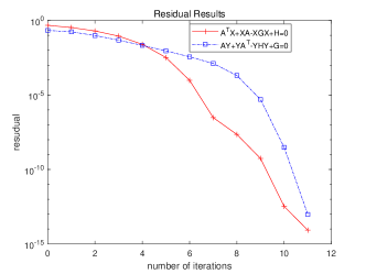
(a) residuals

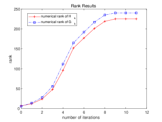
(b) ranks

Figure 2: Normalized residuals and numerical ranks for $n=1357$

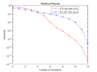
(a) residuals

(b) ranks

Figure 3: Normalized residuals and numerical ranks for $n=5177$

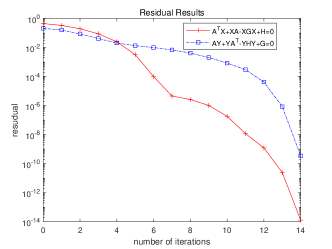
(a) residuals

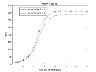
(b) ranks

Figure 4: Normalized residuals and numerical ranks for $n=20209$

We compare the efficiency of the dSDA_t, RKSM, RADI and NKADI for the three test examples. Table 1 displays the numerical results produced by the four algorithms, where $r_{X}$ and “eTime” are respectively the rank of the numerical solution and the associated execution time.

dimension $n=1357$
	dSDAt	RKSM	RADI	NKADI
$\rho_{X}$	$7.19995\times 10^{-15}$	$1.67961\times 10^{-13}$	$2.43172\times 10^{-15}$	$1.18202\times 10^{-15}$
$r_{X}$	$225$	$1147$	$210$	$173$
eTime	$2.09850\times 10^{1}$	$6.98003\times 10^{2}$	$1.53205\times 10^{0}$	$9.21641\times 10^{-1}$
dimension $n=5177$
	dSDAt	RKSM	RADI	NKADI
$\rho_{X}$	$5.20068\times 10^{-14}$	$7.79517\times 10^{-12}$	$7.57244\times 10^{-14}$	$1.41009\times 10^{-15}$
$r_{X}$	$281$	$777$	$216$	$206$
eTime	$2.39945\times 10^{2}$	$1.99366\times 10^{4}$	$4.06343\times 10^{1}$	$9.93228\times 10^{0}$
dimension $n=20209$
	dSDAt	RKSM	RADI	NKADI
$\rho_{X}$	$1.25375\times 10^{-14}$	$1.91847\times 10^{-11}$	$9.25792\times 10^{-15}$	$1.69087\times 10^{-15}$
$r_{X}$	$337$	$2630$	$276$	$222$
eTime	$6.73489\times 10^{3}$	$2.60143\times 10^{4}$	$1.46030\times 10^{3}$	$3.28714\times 10^{2}$

Table 1: Numerical results from different four methods

In these three steel profile cooling examples, the NKADI performs the best, and our dSDA_t is a little worse than the RADI. However, the ratio of the execution time for the dSDA_t and the RADI shows a downtrend as $n$ increases: when $n=1357$, the ratio is $13.6973$; and for $n=5177$, it is $5.9050$, while for $n=20209$, it declines to $4.6120$.

Table 2 shows the numerical results produced by the dSDA_t with five different truncation tolerances, where $tol_{j}=10^{-(2j+4)}\times tol$ ($j=1,\cdots,5$) with “$tol$” being a vector and its entries $tol(i)=\max\{10^{-i},10^{-15}\}$ for $i=1,2,\cdots,20$. In Table 2, “iterations” stands for the required number of the iterations. It follows from Table 2 that with different tolerances in truncation the dSDA_t yield similar satisfactory results, meaning that for the three models our dSDA_t is insensitive to the truncation tolerance.

$n=1357$
	$tol_{1}$	$tol_{2}$	$tol_{3}$	$tol_{4}$	$tol_{5}$
$\rho_{X}$	$7.15828\times 10^{-15}$	$7.09397\times 10^{-15}$	$7.55596\times 10^{-15}$	$7.55596\times 10^{-15}$	$7.55596\times 10^{-15}$
$\rho_{Y}$	$1.55751\times 10^{-12}$	$9.65711\times 10^{-14}$	$9.66872\times 10^{-14}$	$9.66872\times 10^{-14}$	$9.66872\times 10^{-14}$
$r_{X}$	$218$	$225$	$225$	$225$	$225$
$r_{Y}$	$230$	$240$	$241$	$241$	$241$
iterations	$11$	$11$	$11$	$11$	$11$
eTime	$2.10654\times 10^{1}$	$2.22646\times 10^{1}$	$2.22835\times 10^{1}$	$2.24233\times 10^{1}$	$2.22558\times 10^{1}$
$n=5177$
	$tol_{1}$	$tol_{2}$	$tol_{3}$	$tol_{4}$	$tol_{5}$
$\rho_{X}$	$5.17750\times 10^{-14}$	$5.18665\times 10^{-14}$	$5.17608\times 10^{-14}$	$5.17608\times 10^{-14}$	$5.17608\times 10^{-14}$
$\rho_{Y}$	$9.03585\times 10^{-10}$	$9.03585\times 10^{-10}$	$9.03585\times 10^{-10}$	$9.03585\times 10^{-10}$	$9.03585\times 10^{-10}$
$r_{X}$	$265$	$276$	$281$	$281$	$281$
$r_{Y}$	$281$	$298$	$299$	$299$	$299$
iterations	$12$	$12$	$12$	$12$	$12$
eTime	$2.35127\times 10^{2}$	$2.45846\times 10^{2}$	$2.52503\times 10^{2}$	$2.53253\times 10^{2}$	$2.49535\times 10^{2}$
$n=20209$
	$tol_{1}$	$tol_{2}$	$tol_{3}$	$tol_{4}$	$tol_{5}$
$\rho_{X}$	$1.21879\times 10^{-14}$	$1.34771\times 10^{-14}$	$1.37765\times 10^{-14}$	$1.37765\times 10^{-14}$	$1.37765\times 10^{-14}$
$\rho_{Y}$	$3.43638\times 10^{-10}$	$3.43638\times 10^{-10}$	$3.43638\times 10^{-10}$	$3.43638\times 10^{-10}$	$3.43638\times 10^{-10}$
$r_{X}$	$321$	$335$	$336$	$336$	$336$
$r_{Y}$	$341$	$358$	$360$	$360$	$360$
iterations	$14$	$14$	$14$	$14$	$14$
eTime	$7.07405\times 10^{3}$	$7.41030\times 10^{3}$	$7.39546\times 10^{3}$	$7.41256\times 10^{3}$	$7.39824\times 10^{3}$

Table 2: Numerical results with different truncation tolerances

Example 5.2.

We compare further the dSDA_t with the NKADI and RADI. This test set includes $1000$ examples, all of which are randomly generated as follows: firstly we obtain a nonsingular $X$ by the command randn in MATLAB and two diagonal matrices $\Lambda_{1}>0,\Lambda_{2}<0$, whose sizes respectively are $100$ and $3$. The absolute values of all entries of $\Lambda_{1},\Lambda_{2}$ follow the uniform distribution in the interval $(0,1)$. Then we set $A=\frac{1}{100}X\operatorname{diag}(\Lambda_{1},\Lambda_{2})X^{-1}$ and randomly generate $B\in\mathbb{R}^{103\times 3},C\in\mathbb{R}^{3\times 103}$ with randn, with $(A,B)$ being stabilizable and $(A,C)$ detectable.

For those $1000$ random examples, our dSDA_t and the NKADI, which does not perform the Galerkin projection process, converge and produce low rank solutions. On average, the dSDA_t requires $8.4780$ doubling steps for achieving a normalized residual smaller than $10^{-13}$, while the NKADI needs $18.5080$ Newton-Kleinman steps. The NKADI with the Galerkin acceleration produces no result, because it fails to solve some projected CAREs. The RADI fails for all these $1000$ random examples, possibly attributable the unstable $A$ or the choices of shifts. In fact, [3] claims that with the same shifts, the RADI and the Incremental Low-Rank Subspace Iteration [25] are equivalent. The latter achieves convergence when $A$ is stable and satisfies the non-Blaschke condition $\sum_{k=1}^{\infty}\frac{\Re(\alpha_{k})}{1+|\alpha_{k}|^{2}}=-\infty$, where $\alpha_{k}$ are the shifts in each iteration. However, in our test set, $A$ are not stable for all randomly generated examples.

Next with generated $A,B,C$ as above, we scale $B$ and $C$ to one tenth of their sizes, and then apply the NKADI and the dSDA_t to the randomly generated examples. The NKADI with the Galerkin projection still fails, while the NKADI without the Galerkin step achieves convergence only for $26$ examples, even though the maximum iteration number for the Newton-Kleinman and the ADI steps are both set as $1000$. In fact, the NKADI is quadratically convergent provided the initial guess $X_{0}$ is stabilizing. However, for such large random examples, it is difficult to find good initial stabilizing values of $X_{0}$. In the same $1000$ tests, the dSDA_t is effective for $32$% examples within $9.9718$ iterations, and all convergent examples produce low-rank solutions. For those failed examples, the dSDA_t seems to converge within several iterations, then spin out of the convergence. We observe that imbalance in entries in some matrices, possibly leading to ill-conditioning. A balancing technique may cure the problem but we shall leave this research for the future.

In summary, Examples 5.1 and 5.2 illustrate the efficiency and convergence of the dSDA_t for large well-conditioned CAREs, with the method occasionally outperformed by the NKADI and the RADI for problems with stable $A$. However, for examples with unstable $A$, the dSDA_t demonstrates its superiority, without any need for any initial stabilizing $X_{0}$.

6 Conclusions

The classical structure-preserving doubling algorithm (SDA) is an efficient and elegant method for computing the unique symmetric positive semi-definite solution to CAREs of small and medium sizes. However, for large-scale CAREs, it suffers from high computational costs, in terms of execution time and memory requirement. Fortunately, the decoupled structure-preserving doubling algorithm (dSDA) decouples the three iteration recursions, thus improving the efficiency of the SDA for CAREs. Based on the elegant form of the dSDA, we propose a novel truncation technique, which control the ill-conditioning of the kernels of the approximate solutions and their ranks. The resulting algorithm, the truncated dSDA or dSDA_t, computes low-rank approximate solutions efficiently. Furthermore, we analyze the proposed algorithm and prove its convergence. Numerical experiments illustrate the efficiency of the dSDA_t.

Appendix A Proof of Lemma 3.4

We just show the computing details for $L_{2}^{G}$ and $L_{2}^{H}$, from the known $L_{1}^{G}$ and $L_{1}^{H}$. For $L_{j}^{G}$ and $L_{j}^{H}$ with $j\geq 3$, the process is similar. Since

$$E(Y_{2}^{(1)})= \left[I_{4m}+Y_{2}^{(1)}(Y_{2}^{(1)})^{\operatorname{\sf T}}\right]^{-1}$$

$$= \begin{bmatrix}I_{2m}&-2\gamma\Gamma\\ 0&I_{2m}\end{bmatrix}\left[(I_{2m}+Y_{1}Y_{1}^{\operatorname{\sf T}})^{-1}\oplus\Psi_{1}^{-1}\right]\begin{bmatrix}I_{2m}&0\\ -2\gamma\Gamma^{\operatorname{\sf T}}&I_{2m}\end{bmatrix},$$

where $\Gamma:=(I_{2m}+Y_{1}Y_{1}^{\operatorname{\sf T}})^{-1}Y_{1}(T_{1}^{(1)})^{\operatorname{\sf T}}$, $T_{1}^{(1)}=(M_{0}^{G})^{\operatorname{\sf T}}\Omega_{1}M_{0}^{H}$ and $\Psi_{1}:=I_{2m}+Y_{1}Y_{1}^{\operatorname{\sf T}}+4\gamma^{2}T_{1}^{(1)}(I_{2l}+Y_{1}^{\operatorname{\sf T}}Y_{1})^{-1}(T_{1}^{(1)})^{\operatorname{\sf T}}$, then by the definition of $L_{2}^{G}$ in (18) and (29), we have

$$L_{2}^{G} \equiv 2\gamma(\Theta_{1,2}^{G})^{\operatorname{\sf T}}M_{1}^{G}\left[I_{4m}+Y_{2}^{(2)}(Y_{2}^{(2)})^{\operatorname{\sf T}}\right]^{-1}Y_{2}^{(2)}(M_{1}^{H})^{\operatorname{\sf T}}\Theta_{1,2}^{H}\Omega_{2}^{\operatorname{\sf T}}$$

(47) $$=\begin{multlined}2\gamma(\Theta_{1,2}^{G})^{\operatorname{\sf T}}M_{1}^{G}\begin{bmatrix}I_{2m}&-2\gamma\Gamma\\ 0&I_{2m}\end{bmatrix}[E(Y_{1}^{(1)})\oplus\Psi_{1}^{-1}]\begin{bmatrix}I_{2m}&0\\ -2\gamma\Gamma^{\operatorname{\sf T}}&I_{2m}\end{bmatrix}\\ \cdot\begin{bmatrix}0&Y_{1}^{(1)}\\ Y_{1}^{(1)}&2\gamma T_{1}^{(1)}\end{bmatrix}(M_{1}^{H})^{\operatorname{\sf T}}\Theta_{1,2}^{H}\Omega_{2}^{\operatorname{\sf T}}\end{multlined}2\gamma(\Theta_{1,2}^{G})^{\operatorname{\sf T}}M_{1}^{G}\begin{bmatrix}I_{2m}&-2\gamma\Gamma\\ 0&I_{2m}\end{bmatrix}[E(Y_{1}^{(1)})\oplus\Psi_{1}^{-1}]\begin{bmatrix}I_{2m}&0\\ -2\gamma\Gamma^{\operatorname{\sf T}}&I_{2m}\end{bmatrix}\\ \cdot\begin{bmatrix}0&Y_{1}^{(1)}\\ Y_{1}^{(1)}&2\gamma T_{1}^{(1)}\end{bmatrix}(M_{1}^{H})^{\operatorname{\sf T}}\Theta_{1,2}^{H}\Omega_{2}^{\operatorname{\sf T}}$$

(50) $$=\begin{multlined}2\gamma(\Theta_{1,2}^{G})^{\operatorname{\sf T}}\begin{bmatrix}I_{r_{1}^{G}}&R_{12}^{U}\\ 0&R_{2}^{U}\end{bmatrix}\begin{bmatrix}I_{r_{1}^{G}}&-L_{1}^{G}\\ 0&I_{r_{1}^{G}}\end{bmatrix}(I_{2}\otimes M_{0}^{G})[E(Y_{1}^{(1)})\oplus\Psi_{1}^{-1}]\\ \cdot\begin{bmatrix}0&Y_{1}^{(1)}\\ Y_{1}^{(1)}&2\gamma T_{1}^{(1)}F(Y_{1}^{(1)})\end{bmatrix}(I_{2}\otimes M_{0}^{H})^{\operatorname{\sf T}}\begin{bmatrix}I_{r_{1}^{H}}&R_{12}^{V}\\ 0&R_{2}^{V}\end{bmatrix}^{\operatorname{\sf T}}\Theta_{1,2}^{H}\Omega_{2}^{\operatorname{\sf T}}\end{multlined}2\gamma(\Theta_{1,2}^{G})^{\operatorname{\sf T}}\begin{bmatrix}I_{r_{1}^{G}}&R_{12}^{U}\\ 0&R_{2}^{U}\end{bmatrix}\begin{bmatrix}I_{r_{1}^{G}}&-L_{1}^{G}\\ 0&I_{r_{1}^{G}}\end{bmatrix}(I_{2}\otimes M_{0}^{G})[E(Y_{1}^{(1)})\oplus\Psi_{1}^{-1}]\\ \cdot\begin{bmatrix}0&Y_{1}^{(1)}\\ Y_{1}^{(1)}&2\gamma T_{1}^{(1)}F(Y_{1}^{(1)})\end{bmatrix}(I_{2}\otimes M_{0}^{H})^{\operatorname{\sf T}}\begin{bmatrix}I_{r_{1}^{H}}&R_{12}^{V}\\ 0&R_{2}^{V}\end{bmatrix}^{\operatorname{\sf T}}\Theta_{1,2}^{H}\Omega_{2}^{\operatorname{\sf T}}$$

(54) $$=\begin{multlined}2\gamma(\Theta_{1,2}^{G})^{\operatorname{\sf T}}\begin{bmatrix}I_{r_{1}^{G}}&R_{12}^{U}\\ 0&R_{2}^{U}\end{bmatrix}\begin{bmatrix}I_{r_{1}^{G}}&-L_{1}^{G}\\ 0&I_{r_{1}^{G}}\end{bmatrix}\\ \cdot\begin{bmatrix}0&M_{0}^{G}E(Y_{1}^{(1)})Y_{1}^{(1)}(M_{0}^{H})^{\operatorname{\sf T}}\\ M_{0}^{G}\Psi_{1}^{-1}Y_{1}^{(1)}(M_{0}^{H})^{\operatorname{\sf T}}&2\gamma M_{0}^{G}\Psi_{1}^{-1}T_{1}^{(1)}F(Y_{1}^{(1)})(M_{0}^{H})^{\operatorname{\sf T}}\end{bmatrix}\\ \cdot\begin{bmatrix}I_{r_{1}^{H}}&R_{12}^{V}\\ 0&R_{2}^{V}\end{bmatrix}^{\operatorname{\sf T}}\Theta_{1,2}^{H}\Omega_{2}^{\operatorname{\sf T}}\end{multlined}2\gamma(\Theta_{1,2}^{G})^{\operatorname{\sf T}}\begin{bmatrix}I_{r_{1}^{G}}&R_{12}^{U}\\ 0&R_{2}^{U}\end{bmatrix}\begin{bmatrix}I_{r_{1}^{G}}&-L_{1}^{G}\\ 0&I_{r_{1}^{G}}\end{bmatrix}\\ \cdot\begin{bmatrix}0&M_{0}^{G}E(Y_{1}^{(1)})Y_{1}^{(1)}(M_{0}^{H})^{\operatorname{\sf T}}\\ M_{0}^{G}\Psi_{1}^{-1}Y_{1}^{(1)}(M_{0}^{H})^{\operatorname{\sf T}}&2\gamma M_{0}^{G}\Psi_{1}^{-1}T_{1}^{(1)}F(Y_{1}^{(1)})(M_{0}^{H})^{\operatorname{\sf T}}\end{bmatrix}\\ \cdot\begin{bmatrix}I_{r_{1}^{H}}&R_{12}^{V}\\ 0&R_{2}^{V}\end{bmatrix}^{\operatorname{\sf T}}\Theta_{1,2}^{H}\Omega_{2}^{\operatorname{\sf T}}$$

(58) $$=\begin{multlined}2\gamma(\Theta_{1,2}^{G})^{\operatorname{\sf T}}\begin{bmatrix}I_{r_{1}^{G}}&R_{12}^{U}\\ 0&R_{2}^{U}\end{bmatrix}\begin{bmatrix}I_{r_{1}^{G}}&-L_{1}^{G}\\ 0&I_{r_{1}^{G}}\end{bmatrix}\\ \cdot\begin{bmatrix}0&\Sigma_{1,1}^{G}K_{1}^{G}\Sigma_{1,1}^{H}\\ M_{0}^{G}\Psi_{1}^{-1}Y_{1}^{(1)}(M_{0}^{H})^{\operatorname{\sf T}}&2\gamma M_{0}^{G}\Psi_{1}^{-1}T_{1}^{(1)}F(Y_{1}^{(1)})(M_{0}^{H})^{\operatorname{\sf T}}\end{bmatrix}\\ \cdot\begin{bmatrix}I_{r_{1}^{H}}&R_{12}^{V}\\ 0&R_{2}^{V}\end{bmatrix}^{\operatorname{\sf T}}\Theta_{1,2}^{H}\Omega_{2}^{\operatorname{\sf T}},\end{multlined}2\gamma(\Theta_{1,2}^{G})^{\operatorname{\sf T}}\begin{bmatrix}I_{r_{1}^{G}}&R_{12}^{U}\\ 0&R_{2}^{U}\end{bmatrix}\begin{bmatrix}I_{r_{1}^{G}}&-L_{1}^{G}\\ 0&I_{r_{1}^{G}}\end{bmatrix}\\ \cdot\begin{bmatrix}0&\Sigma_{1,1}^{G}K_{1}^{G}\Sigma_{1,1}^{H}\\ M_{0}^{G}\Psi_{1}^{-1}Y_{1}^{(1)}(M_{0}^{H})^{\operatorname{\sf T}}&2\gamma M_{0}^{G}\Psi_{1}^{-1}T_{1}^{(1)}F(Y_{1}^{(1)})(M_{0}^{H})^{\operatorname{\sf T}}\end{bmatrix}\\ \cdot\begin{bmatrix}I_{r_{1}^{H}}&R_{12}^{V}\\ 0&R_{2}^{V}\end{bmatrix}^{\operatorname{\sf T}}\Theta_{1,2}^{H}\Omega_{2}^{\operatorname{\sf T}},$$

where $E(Y_{1}^{(1)}):=[I_{2m}+Y_{1}^{(1)}(Y_{1}^{(1)})^{\operatorname{\sf T}}]^{-1}$, $F(Y_{1}^{(1)}):=[I_{2l}+(Y_{1}^{(1)})^{\operatorname{\sf T}}Y_{1}^{(1)}]^{-1}$. We next calculate some submatrices in (58). By (7), (29) and $M_{0}^{H}=(\Theta_{1,1}^{H})^{\operatorname{\sf T}}R_{1}^{V}P_{1}^{V}$, we deduce

$$T_{1}^{(1)}F(Y_{1}^{(1)})(T_{1}^{(1)})^{\operatorname{\sf T}}=(M_{0}^{G})^{\operatorname{\sf T}}\Omega_{1}M_{0}^{H}F(Y_{1}^{(1)})(M_{0}^{H})^{\operatorname{\sf T}}\Omega_{1}^{\operatorname{\sf T}}M_{0}^{G}$$

$$= (M_{0}^{G})^{\operatorname{\sf T}}\Omega_{1}M_{0}^{H}V_{1}^{Y}\left[I_{2l}+(\Sigma_{1}^{Y})^{\operatorname{\sf T}}\Sigma_{1}^{Y}\right]^{-1}(V_{1}^{Y})^{\operatorname{\sf T}}(M_{0}^{H})^{\operatorname{\sf T}}\Omega_{1}^{\operatorname{\sf T}}M_{0}^{G}$$

$$= (M_{0}^{G})^{\operatorname{\sf T}}\Omega_{1}(\Theta_{1,1}^{H})^{\operatorname{\sf T}}R_{1}^{V}P_{1}^{V}V_{1}^{Y}\left[I_{2l}+(\Sigma_{1}^{Y})^{\operatorname{\sf T}}\Sigma_{1}^{Y}\right]^{-1}(V_{1}^{Y})^{\operatorname{\sf T}}(P_{1}^{V})^{\operatorname{\sf T}}(R_{1}^{V})^{\operatorname{\sf T}}\Theta_{1,1}^{H}\Omega_{1}^{\operatorname{\sf T}}M_{0}^{G}$$

$$= (M_{0}^{G})^{\operatorname{\sf T}}\Omega_{1}(\Theta_{1,1}^{H})^{\operatorname{\sf T}}\Theta_{1}^{H}(\Sigma_{1}^{H})^{2}(\Theta_{1}^{H})^{\operatorname{\sf T}}\Theta_{1,1}^{H}\Omega_{1}^{\operatorname{\sf T}}M_{0}^{G}\equiv(M_{0}^{G})^{\operatorname{\sf T}}\Omega_{1}(\Sigma_{1,1}^{H})^{2}\Omega_{1}^{\operatorname{\sf T}}M_{0}^{G},$$

implying that $\Psi_{1}=I_{2m}+Y_{1}Y_{1}^{\operatorname{\sf T}}+4\gamma^{2}(M_{0}^{G})^{\operatorname{\sf T}}\Omega_{1}(\Sigma_{1,1}^{H})^{2}\Omega_{1}^{\operatorname{\sf T}}M_{0}^{G}$. Because

$$M_{0}^{G}E(Y_{1}^{(1)})(M_{0}^{G})^{\operatorname{\sf T}} =(\Theta_{1,1}^{G})^{\operatorname{\sf T}}\Theta_{1}^{G}(\Sigma_{1}^{G})^{2}(\Theta_{1}^{G})^{\operatorname{\sf T}}\Theta_{1,1}^{G}\equiv(\Sigma_{1,1}^{G})^{2},$$

$$M_{0}^{H}F(Y_{1}^{(1)})(M_{0}^{H})^{\operatorname{\sf T}} =(\Theta_{1,1}^{H})^{\operatorname{\sf T}}\Theta_{1}^{H}(\Sigma_{1}^{H})^{2}(\Theta_{1}^{H})^{\operatorname{\sf T}}\Theta_{1,1}^{H}\equiv(\Sigma_{1,1}^{H})^{2},$$

then by (29) and the SMWF, we have

$$M_{0}^{G}\Psi_{1}^{-1}Y_{1}^{(1)}(M_{0}^{H})^{\operatorname{\sf T}}$$

$$= M_{0}^{G}\left[I_{2m}+Y_{1}^{(1)}(Y_{1}^{(1)})^{\operatorname{\sf T}}+4\gamma^{2}(M_{0}^{G})^{\operatorname{\sf T}}\Omega_{1}(\Sigma_{1,1}^{H})^{2}\Omega_{1}^{\operatorname{\sf T}}M_{0}^{G}\right]^{-1}Y_{1}^{(1)}(M_{0}^{H})^{\operatorname{\sf T}}$$

(61) $$= \begin{multlined}M_{0}^{G}E(Y_{1}^{(1)})Y_{1}^{(1)}(M_{0}^{H})^{\operatorname{\sf T}}-4\gamma^{2}M_{0}^{G}E(Y_{1}^{(1)})(M_{0}^{G})^{\operatorname{\sf T}}\Omega_{1}\\ \cdot\left[\left(\Sigma_{1,1}^{H}\right)^{-2}+4\gamma^{2}\Omega_{1}^{\operatorname{\sf T}}M_{0}^{G}E(Y_{1}^{(1)})(M_{0}^{G})^{\operatorname{\sf T}}\Omega_{1}\right]^{-1}\Omega_{1}^{\operatorname{\sf T}}M_{0}^{G}E(Y_{1}^{(1)})Y_{1}^{(1)}(M_{0}^{H})^{\operatorname{\sf T}}\end{multlined}M_{0}^{G}E(Y_{1}^{(1)})Y_{1}^{(1)}(M_{0}^{H})^{\operatorname{\sf T}}-4\gamma^{2}M_{0}^{G}E(Y_{1}^{(1)})(M_{0}^{G})^{\operatorname{\sf T}}\Omega_{1}\\ \cdot\left[\left(\Sigma_{1,1}^{H}\right)^{-2}+4\gamma^{2}\Omega_{1}^{\operatorname{\sf T}}M_{0}^{G}E(Y_{1}^{(1)})(M_{0}^{G})^{\operatorname{\sf T}}\Omega_{1}\right]^{-1}\Omega_{1}^{\operatorname{\sf T}}M_{0}^{G}E(Y_{1}^{(1)})Y_{1}^{(1)}(M_{0}^{H})^{\operatorname{\sf T}}$$

$$= \Sigma_{1,1}^{G}K_{1}^{G}\Sigma_{1,1}^{H}-4\gamma^{2}(\Sigma_{1,1}^{G})^{2}\Omega_{1}\left[\left(\Sigma_{1,1}^{H}\right)^{-2}+4\gamma^{2}\Omega_{1}^{\operatorname{\sf T}}(\Sigma_{1,1}^{G})^{2}\Omega_{1}\right]^{-1}\Omega_{1}^{\operatorname{\sf T}}\Sigma_{1,1}^{G}K_{1}^{G}\Sigma_{1,1}^{H}$$

$$= \left\{I_{r_{1}^{G}}-4\gamma^{2}(\Sigma_{1,1}^{G})^{2}\Omega_{1}\left[\left(\Sigma_{1,1}^{H}\right)^{-2}+4\gamma^{2}\Omega_{1}^{\operatorname{\sf T}}(\Sigma_{1,1}^{G})^{2}\Omega_{1}\right]^{-1}\Omega_{1}^{\operatorname{\sf T}}\right\}\Sigma_{1,1}^{G}K_{1}^{G}\Sigma_{1,1}^{H}$$

(63) $$= \begin{multlined}\left\{I_{r_{1}^{G}}-4\gamma^{2}(\Sigma_{1,1}^{G})^{2}\Omega_{1}\Sigma_{1,1}^{H}[I_{r_{1}^{H}}+4\gamma^{2}\Sigma_{1,1}^{H}\Omega_{1}^{\operatorname{\sf T}}(\Sigma_{1,1}^{G})^{2}\Omega_{1}\Sigma_{1,1}^{H}]^{-1}\Sigma_{1,1}^{H}\Omega_{1}^{\operatorname{\sf T}}\right\}\Sigma_{1,1}^{G}K_{1}^{G}\Sigma_{1,1}^{H}\end{multlined}\left\{I_{r_{1}^{G}}-4\gamma^{2}(\Sigma_{1,1}^{G})^{2}\Omega_{1}\Sigma_{1,1}^{H}[I_{r_{1}^{H}}+4\gamma^{2}\Sigma_{1,1}^{H}\Omega_{1}^{\operatorname{\sf T}}(\Sigma_{1,1}^{G})^{2}\Omega_{1}\Sigma_{1,1}^{H}]^{-1}\Sigma_{1,1}^{H}\Omega_{1}^{\operatorname{\sf T}}\right\}\Sigma_{1,1}^{G}K_{1}^{G}\Sigma_{1,1}^{H}$$

(65) $$= \begin{multlined}\left\{I_{r_{1}^{G}}-4\gamma^{2}[I_{r_{1}^{G}}+4\gamma^{2}(\Sigma_{1,1}^{G})^{2}\Omega_{1}(\Sigma_{1,1}^{H})^{2}\Omega_{1}^{\operatorname{\sf T}}]^{-1}(\Sigma_{1,1}^{G})^{2}\Omega_{1}(\Sigma_{1,1}^{H})^{2}\Omega_{1}^{\operatorname{\sf T}}\right\}\Sigma_{1,1}^{G}K_{1}^{G}\Sigma_{1,1}^{H}\end{multlined}\left\{I_{r_{1}^{G}}-4\gamma^{2}[I_{r_{1}^{G}}+4\gamma^{2}(\Sigma_{1,1}^{G})^{2}\Omega_{1}(\Sigma_{1,1}^{H})^{2}\Omega_{1}^{\operatorname{\sf T}}]^{-1}(\Sigma_{1,1}^{G})^{2}\Omega_{1}(\Sigma_{1,1}^{H})^{2}\Omega_{1}^{\operatorname{\sf T}}\right\}\Sigma_{1,1}^{G}K_{1}^{G}\Sigma_{1,1}^{H}$$

$$= \left[I_{r_{1}^{G}}+4\gamma^{2}(\Sigma_{1,1}^{G})^{2}\Omega_{1}(\Sigma_{1,1}^{H})^{2}\Omega_{1}^{\operatorname{\sf T}}\right]^{-1}\Sigma_{1,1}^{G}K_{1}^{G}\Sigma_{1,1}^{H}$$

$$= \Sigma_{1,1}^{G}\left[I_{r_{1}^{G}}+4\gamma^{2}\Sigma_{1,1}^{G}\Omega_{1}(\Sigma_{1,1}^{H})^{2}\Omega_{1}^{\operatorname{\sf T}}\Sigma_{1,1}^{G}\right]^{-1}K_{1}^{G}\Sigma_{1,1}^{H}$$

$$= \Sigma_{1,1}^{G}\left[I_{r_{1}^{G}}+4\gamma^{2}U_{2}^{Y}\Sigma_{2}^{Y}(\Sigma_{2}^{Y})^{\operatorname{\sf T}}(U_{2}^{Y})^{\operatorname{\sf T}}\right]^{-1}K_{1}^{G}\Sigma_{1,1}^{H}$$

$$= \Sigma_{1,1}^{G}U_{2}^{Y}\left(I_{r_{1}^{G}}+4\gamma^{2}\Sigma_{2}^{Y}(\Sigma_{2}^{Y})^{\operatorname{\sf T}}\right)^{-1}(U_{2}^{Y})^{\operatorname{\sf T}}K_{1}^{G}\Sigma_{1,1}^{H}$$

(66) $$= \Sigma_{1,1}^{G}U_{2}^{Y}(\Upsilon_{2}^{G})^{-1}(U_{2}^{Y})^{\operatorname{\sf T}}K_{1}^{G}\Sigma_{1,1}^{H}:=Z_{21}\equiv\Sigma_{1,1}^{G}U_{2}^{Y}(\Upsilon_{2}^{G})^{-1/2}\widehat{Z}_{21},$$

where $\Upsilon_{2}^{G}=I_{r_{1}^{G}}+4\gamma^{2}\Sigma_{2}^{Y}(\Sigma_{2}^{Y})^{\operatorname{\sf T}}$ and $\widehat{Z}_{21}:=(\Upsilon_{2}^{G})^{-1/2}(U_{2}^{Y})^{\operatorname{\sf T}}K_{1}^{G}\Sigma_{1,1}^{H}$. We also have

$$M_{0}^{G}\Psi_{1}^{-1}T_{1}^{(1)}F(Y_{1}^{(1)})(M_{0}^{H})^{\operatorname{\sf T}}$$

$$= M_{0}^{G}\left[I_{2m}+Y_{1}^{(1)}(Y_{1}^{(1)})^{\operatorname{\sf T}}+4\gamma^{2}(M_{0}^{G})^{\operatorname{\sf T}}\Omega_{1}(\Sigma_{1,1}^{H})^{2}\Omega_{1}^{\operatorname{\sf T}}M_{0}^{G}\right]^{-1}T_{1}^{(1)}F(Y_{1}^{(1)})(M_{0}^{H})^{\operatorname{\sf T}}$$

(69) $$= \begin{multlined}M_{0}^{G}E(Y_{1}^{(1)})T_{1}^{(1)}F(Y_{1}^{(1)})(M_{0}^{H})^{\operatorname{\sf T}}-4\gamma^{2}M_{0}^{G}E(Y_{1}^{(1)})(M_{0}^{G})^{\operatorname{\sf T}}\Omega_{1}\\ \cdot\left[\left(\Sigma_{1,1}^{H}\right)^{-2}+4\gamma^{2}\Omega_{1}^{\operatorname{\sf T}}M_{0}^{G}E(Y_{1}^{(1)})(M_{0}^{G})^{\operatorname{\sf T}}\Omega_{1}\right]^{-1}\Omega_{1}^{\operatorname{\sf T}}M_{0}^{G}E(Y_{1}^{(1)})T_{1}^{(1)}F(Y_{1}^{(1)})(M_{0}^{H})^{\operatorname{\sf T}}\end{multlined}M_{0}^{G}E(Y_{1}^{(1)})T_{1}^{(1)}F(Y_{1}^{(1)})(M_{0}^{H})^{\operatorname{\sf T}}-4\gamma^{2}M_{0}^{G}E(Y_{1}^{(1)})(M_{0}^{G})^{\operatorname{\sf T}}\Omega_{1}\\ \cdot\left[\left(\Sigma_{1,1}^{H}\right)^{-2}+4\gamma^{2}\Omega_{1}^{\operatorname{\sf T}}M_{0}^{G}E(Y_{1}^{(1)})(M_{0}^{G})^{\operatorname{\sf T}}\Omega_{1}\right]^{-1}\Omega_{1}^{\operatorname{\sf T}}M_{0}^{G}E(Y_{1}^{(1)})T_{1}^{(1)}F(Y_{1}^{(1)})(M_{0}^{H})^{\operatorname{\sf T}}$$

(72) $$= \begin{multlined}M_{0}^{G}E(Y_{1}^{(1)})(M_{0}^{G})^{\operatorname{\sf T}}\Omega_{1}M_{0}^{H}F(Y_{1}^{(1)})(M_{0}^{H})^{\operatorname{\sf T}}-4\gamma^{2}(\Sigma_{1,1}^{G})^{2}\Omega_{1}\\ \cdot\left[\left(\Sigma_{1,1}^{H}\right)^{-2}+4\gamma^{2}\Omega_{1}^{\operatorname{\sf T}}(\Sigma_{1,1}^{G})^{2}\Omega_{1}\right]^{-1}\Omega_{1}^{\operatorname{\sf T}}M_{0}^{G}E(Y_{1}^{(1)})(M_{0}^{G})^{\operatorname{\sf T}}\Omega_{1}M_{0}^{H}F(Y_{1}^{(1)})(M_{0}^{H})^{\operatorname{\sf T}}\end{multlined}M_{0}^{G}E(Y_{1}^{(1)})(M_{0}^{G})^{\operatorname{\sf T}}\Omega_{1}M_{0}^{H}F(Y_{1}^{(1)})(M_{0}^{H})^{\operatorname{\sf T}}-4\gamma^{2}(\Sigma_{1,1}^{G})^{2}\Omega_{1}\\ \cdot\left[\left(\Sigma_{1,1}^{H}\right)^{-2}+4\gamma^{2}\Omega_{1}^{\operatorname{\sf T}}(\Sigma_{1,1}^{G})^{2}\Omega_{1}\right]^{-1}\Omega_{1}^{\operatorname{\sf T}}M_{0}^{G}E(Y_{1}^{(1)})(M_{0}^{G})^{\operatorname{\sf T}}\Omega_{1}M_{0}^{H}F(Y_{1}^{(1)})(M_{0}^{H})^{\operatorname{\sf T}}$$

(75) $$= \begin{multlined}(\Sigma_{1,1}^{G})^{2}\Omega_{1}(\Sigma_{1,1}^{H})^{2}-4\gamma^{2}(\Sigma_{1,1}^{G})^{2}\Omega_{1}\left[(\Sigma_{1,1}^{H})^{-2}+4\gamma^{2}\Omega_{1}^{\operatorname{\sf T}}(\Sigma_{1,1}^{G})^{2}\Omega_{1}\right]^{-1}\\ \cdot\Omega_{1}^{\operatorname{\sf T}}(\Sigma_{1,1}^{G})^{2}\Omega_{1}(\Sigma_{1,1}^{H})^{2}\end{multlined}(\Sigma_{1,1}^{G})^{2}\Omega_{1}(\Sigma_{1,1}^{H})^{2}-4\gamma^{2}(\Sigma_{1,1}^{G})^{2}\Omega_{1}\left[(\Sigma_{1,1}^{H})^{-2}+4\gamma^{2}\Omega_{1}^{\operatorname{\sf T}}(\Sigma_{1,1}^{G})^{2}\Omega_{1}\right]^{-1}\\ \cdot\Omega_{1}^{\operatorname{\sf T}}(\Sigma_{1,1}^{G})^{2}\Omega_{1}(\Sigma_{1,1}^{H})^{2}$$

$$= \left[I_{r_{1}^{G}}+4\gamma^{2}(\Sigma_{1,1}^{G})^{2}\Omega_{1}(\Sigma_{1,1}^{H})^{2}\Omega_{1}^{\operatorname{\sf T}}\right]^{-1}(\Sigma_{1,1}^{G})^{2}\Omega_{1}(\Sigma_{1,1}^{H})^{2}$$

$$= \Sigma_{1,1}^{G}\left[I_{r_{1}^{G}}+4\gamma^{2}\Sigma_{1,1}^{G}\Omega_{1}(\Sigma_{1,1}^{H})^{2}\Omega_{1}^{\operatorname{\sf T}}\Sigma_{1,1}^{G}\right]^{-1}\Sigma_{1,1}^{G}\Omega_{1}(\Sigma_{1,1}^{H})^{2}$$

(76) $$= \Sigma_{1,1}^{G}U_{2}^{Y}(\Upsilon_{2}^{G})^{-1}(U_{2}^{Y})^{\operatorname{\sf T}}\Sigma_{1,1}^{G}\Omega_{1}(\Sigma_{1,1}^{H})^{2}:=Z_{22}\equiv\Sigma_{1,1}^{G}U_{2}^{Y}(\Upsilon_{2}^{G})^{-1/2}\widehat{Z}_{22},$$

where $\widehat{Z}_{22}:=(\Upsilon_{2}^{G})^{-1/2}(U_{2}^{Y})^{\operatorname{\sf T}}\Sigma_{1,1}^{G}\Omega_{1}(\Sigma_{1,1}^{H})^{2}$. By (58), (66) and (76) it consequently holds that

$$L_{2}^{G} =2\gamma(\Theta_{1,2}^{G})^{\operatorname{\sf T}}\begin{bmatrix}I_{r_{1}^{G}}&R_{12}^{U}\\ 0&R_{2}^{U}\end{bmatrix}\begin{bmatrix}I_{r_{1}^{G}}&-L_{1}^{G}\\ 0&I_{r_{1}^{G}}\end{bmatrix}\begin{bmatrix}0&\Sigma_{1,1}^{G}K_{1}^{G}\Sigma_{1,1}^{H}\\ Z_{21}&2\gamma Z_{22}\end{bmatrix}\begin{bmatrix}I_{r_{1}^{H}}&R_{12}^{V}\\ 0&R_{2}^{V}\end{bmatrix}^{\operatorname{\sf T}}\Theta_{1,2}^{H}\Omega_{2}^{\operatorname{\sf T}}$$

$$=\begin{multlined}2\gamma(\Theta_{1,2}^{G})^{\operatorname{\sf T}}\begin{bmatrix}I_{r_{1}^{G}}&R_{12}^{U}\\ 0&R_{2}^{U}\end{bmatrix}\begin{bmatrix}I_{r_{1}^{G}}&-L_{1}^{G}\\ 0&I_{r_{1}^{G}}\end{bmatrix}\left[\Sigma_{1,1}^{G}\oplus\Sigma_{1,1}^{G}U_{2}^{Y}(\Upsilon_{2}^{G})^{-1/2}\right]\\ \cdot\begin{bmatrix}0&K_{1}^{G}\Sigma_{1,1}^{H}\\ \widehat{Z}_{21}&2\gamma\widehat{Z}_{22}\end{bmatrix}\begin{bmatrix}I_{r_{1}^{H}}&R_{12}^{V}\\ 0&R_{2}^{V}\end{bmatrix}^{\operatorname{\sf T}}\Theta_{1,2}^{H}\Omega_{2}^{\operatorname{\sf T}}.\end{multlined}2\gamma(\Theta_{1,2}^{G})^{\operatorname{\sf T}}\begin{bmatrix}I_{r_{1}^{G}}&R_{12}^{U}\\ 0&R_{2}^{U}\end{bmatrix}\begin{bmatrix}I_{r_{1}^{G}}&-L_{1}^{G}\\ 0&I_{r_{1}^{G}}\end{bmatrix}\left[\Sigma_{1,1}^{G}\oplus\Sigma_{1,1}^{G}U_{2}^{Y}(\Upsilon_{2}^{G})^{-1/2}\right]\\ \cdot\begin{bmatrix}0&K_{1}^{G}\Sigma_{1,1}^{H}\\ \widehat{Z}_{21}&2\gamma\widehat{Z}_{22}\end{bmatrix}\begin{bmatrix}I_{r_{1}^{H}}&R_{12}^{V}\\ 0&R_{2}^{V}\end{bmatrix}^{\operatorname{\sf T}}\Theta_{1,2}^{H}\Omega_{2}^{\operatorname{\sf T}}.$$

Moreover, by (11), we get

$$L_{2} =2\gamma(\Theta_{1,2}^{G})^{\operatorname{\sf T}}\Theta_{2}^{G}\Sigma_{2}^{G}(\Phi_{2}^{G})^{\operatorname{\sf T}}\begin{bmatrix}0&K_{1}^{G}\Sigma_{1,1}^{H}\\ \widehat{Z}_{21}&2\gamma\widehat{Z}_{22}\end{bmatrix}\begin{bmatrix}I_{r_{1}^{H}}&R_{12}^{V}\\ 0&R_{2}^{V}\end{bmatrix}^{\operatorname{\sf T}}\Theta_{1,2}^{H}\Omega_{2}^{\operatorname{\sf T}}$$

$$=\begin{multlined}2\gamma\Sigma_{1,2}^{G}(\Phi_{1,2}^{G})^{\operatorname{\sf T}}\begin{bmatrix}0&K_{1}^{G}\Sigma_{1,1}^{H}\\ \widehat{Z}_{21}&2\gamma\widehat{Z}_{22}\end{bmatrix}\begin{bmatrix}I_{r_{1}^{H}}&L_{1}^{H}\\ 0&I_{r_{1}^{H}}\end{bmatrix}^{\operatorname{\sf T}}\\ \cdot\left[(\Sigma_{1,1}^{H})^{-1}\oplus(\Sigma_{1,1}^{H})^{-1}V_{2}^{Y}(\Upsilon_{2}^{H})^{1/2}\right]\left[\Sigma_{1,1}^{H}\oplus(\Upsilon_{2}^{H})^{-1/2}(V_{2}^{Y})^{\operatorname{\sf T}}\Sigma_{1,1}^{H}\right]\\ \cdot\begin{bmatrix}I_{r_{1}^{H}}&-L_{1}^{H}\\ 0&I_{r_{1}^{H}}\end{bmatrix}^{\operatorname{\sf T}}\begin{bmatrix}I_{r_{1}^{H}}&R_{12}^{V}\\ 0&R_{2}^{V}\end{bmatrix}^{\operatorname{\sf T}}\Theta_{1,2}^{H}\Omega_{2}^{\operatorname{\sf T}}\end{multlined}2\gamma\Sigma_{1,2}^{G}(\Phi_{1,2}^{G})^{\operatorname{\sf T}}\begin{bmatrix}0&K_{1}^{G}\Sigma_{1,1}^{H}\\ \widehat{Z}_{21}&2\gamma\widehat{Z}_{22}\end{bmatrix}\begin{bmatrix}I_{r_{1}^{H}}&L_{1}^{H}\\ 0&I_{r_{1}^{H}}\end{bmatrix}^{\operatorname{\sf T}}\\ \cdot\left[(\Sigma_{1,1}^{H})^{-1}\oplus(\Sigma_{1,1}^{H})^{-1}V_{2}^{Y}(\Upsilon_{2}^{H})^{1/2}\right]\left[\Sigma_{1,1}^{H}\oplus(\Upsilon_{2}^{H})^{-1/2}(V_{2}^{Y})^{\operatorname{\sf T}}\Sigma_{1,1}^{H}\right]\\ \cdot\begin{bmatrix}I_{r_{1}^{H}}&-L_{1}^{H}\\ 0&I_{r_{1}^{H}}\end{bmatrix}^{\operatorname{\sf T}}\begin{bmatrix}I_{r_{1}^{H}}&R_{12}^{V}\\ 0&R_{2}^{V}\end{bmatrix}^{\operatorname{\sf T}}\Theta_{1,2}^{H}\Omega_{2}^{\operatorname{\sf T}}$$

$$=\begin{multlined}2\gamma\Sigma_{1,2}^{G}(\Phi_{1,2}^{G})^{\operatorname{\sf T}}\begin{bmatrix}0&K_{1}^{G}\Sigma_{1,1}^{H}\\ \widehat{Z}_{21}&2\gamma\widehat{Z}_{22}\end{bmatrix}\begin{bmatrix}I_{r_{1}^{H}}&L_{1}^{H}\\ 0&I_{r_{1}^{H}}\end{bmatrix}^{\operatorname{\sf T}}\\ \cdot\left[(\Sigma_{1,1}^{H})^{-1}\oplus(\Sigma_{1,1}^{H})^{-1}V_{2}^{Y}(\Upsilon_{2}^{H})^{1/2}\right]\Phi_{2}^{H}\Sigma_{2}^{H}(\Theta_{2}^{H})^{\operatorname{\sf T}}\Theta_{1,2}^{H}\Omega_{2}^{\operatorname{\sf T}}\end{multlined}2\gamma\Sigma_{1,2}^{G}(\Phi_{1,2}^{G})^{\operatorname{\sf T}}\begin{bmatrix}0&K_{1}^{G}\Sigma_{1,1}^{H}\\ \widehat{Z}_{21}&2\gamma\widehat{Z}_{22}\end{bmatrix}\begin{bmatrix}I_{r_{1}^{H}}&L_{1}^{H}\\ 0&I_{r_{1}^{H}}\end{bmatrix}^{\operatorname{\sf T}}\\ \cdot\left[(\Sigma_{1,1}^{H})^{-1}\oplus(\Sigma_{1,1}^{H})^{-1}V_{2}^{Y}(\Upsilon_{2}^{H})^{1/2}\right]\Phi_{2}^{H}\Sigma_{2}^{H}(\Theta_{2}^{H})^{\operatorname{\sf T}}\Theta_{1,2}^{H}\Omega_{2}^{\operatorname{\sf T}}$$

$$=\begin{multlined}2\gamma\Sigma_{1,2}^{G}(\Phi_{1,2}^{G})^{\operatorname{\sf T}}\begin{bmatrix}0&K_{1}^{G}\Sigma_{1,1}^{H}\\ \widehat{Z}_{21}&2\gamma\widehat{Z}_{22}\end{bmatrix}\begin{bmatrix}I_{r_{1}^{H}}&L_{1}^{H}\\ 0&I_{r_{1}^{H}}\end{bmatrix}^{\operatorname{\sf T}}\\ \cdot\left[(\Sigma_{1,1}^{H})^{-1}\oplus(\Sigma_{1,1}^{H})^{-1}V_{2}^{Y}(\Upsilon_{2}^{H})^{1/2}\right]\Phi_{1,2}^{H}\Sigma_{1,2}^{H}\Omega_{2}^{\operatorname{\sf T}}\end{multlined}2\gamma\Sigma_{1,2}^{G}(\Phi_{1,2}^{G})^{\operatorname{\sf T}}\begin{bmatrix}0&K_{1}^{G}\Sigma_{1,1}^{H}\\ \widehat{Z}_{21}&2\gamma\widehat{Z}_{22}\end{bmatrix}\begin{bmatrix}I_{r_{1}^{H}}&L_{1}^{H}\\ 0&I_{r_{1}^{H}}\end{bmatrix}^{\operatorname{\sf T}}\\ \cdot\left[(\Sigma_{1,1}^{H})^{-1}\oplus(\Sigma_{1,1}^{H})^{-1}V_{2}^{Y}(\Upsilon_{2}^{H})^{1/2}\right]\Phi_{1,2}^{H}\Sigma_{1,2}^{H}\Omega_{2}^{\operatorname{\sf T}}$$

where $\Upsilon_{2}^{H}=I_{r_{1}^{H}}+4\gamma^{2}(\Sigma_{2}^{Y})^{\operatorname{\sf T}}\Sigma_{2}^{Y}$.

We further deduce that $K_{1}^{G}\Sigma_{1,1}^{H}(L_{1}^{H})^{\operatorname{\sf T}}(\Sigma_{1,1}^{H})^{-1}=2\gamma K_{1}^{G}\Sigma_{1,1}^{H}\Omega_{1}^{\operatorname{\sf T}}\Sigma_{1,1}^{G}K_{1}^{G}$,

$$\widehat{Z}_{21}(\Sigma_{1,1}^{H})^{-1}+2\gamma\widehat{Z}_{22}(L_{1}^{H})^{\operatorname{\sf T}}(\Sigma_{1,1}^{H})^{-1}$$

$$= \begin{multlined}(\Upsilon_{2}^{G})^{-1/2}(U_{2}^{Y})^{\operatorname{\sf T}}K_{1}^{G}+4\gamma^{2}(\Upsilon_{2}^{G})^{-1/2}(U_{2}^{Y})^{\operatorname{\sf T}}\Sigma_{1,1}^{G}\Omega_{1}(\Sigma_{1,1}^{H})^{2}\Omega_{1}^{\operatorname{\sf T}}\Sigma_{1,1}^{G}K_{1}^{G}\end{multlined}(\Upsilon_{2}^{G})^{-1/2}(U_{2}^{Y})^{\operatorname{\sf T}}K_{1}^{G}+4\gamma^{2}(\Upsilon_{2}^{G})^{-1/2}(U_{2}^{Y})^{\operatorname{\sf T}}\Sigma_{1,1}^{G}\Omega_{1}(\Sigma_{1,1}^{H})^{2}\Omega_{1}^{\operatorname{\sf T}}\Sigma_{1,1}^{G}K_{1}^{G}$$

$$= (\Upsilon_{2}^{G})^{-1/2}(U_{2}^{Y})^{\operatorname{\sf T}}\left[I_{r_{1}^{G}}+4\gamma^{2}\Sigma_{1,1}^{G}\Omega_{1}(\Sigma_{1,1}^{H})^{2}\Omega_{1}^{\operatorname{\sf T}}\Sigma_{1,1}^{G}\right]K_{1}^{G}$$

$$= (\Upsilon_{2}^{G})^{-1/2}(U_{2}^{Y})^{\operatorname{\sf T}}U_{2}^{Y}\Upsilon_{2}^{G}(U_{2}^{Y})^{\operatorname{\sf T}}K_{1}^{G}\equiv(\Upsilon_{2}^{G})^{1/2}(U_{2}^{Y})^{\operatorname{\sf T}}K_{1}^{G},$$

and

$$\widehat{Z}_{22}(\Sigma_{1,1}^{H})^{-1}V_{2}^{Y}(\Upsilon_{2}^{H})^{1/2}=(\Upsilon_{2}^{G})^{-1/2}(U_{2}^{Y})^{\operatorname{\sf T}}\Sigma_{1,1}^{G}\Omega_{1}\Sigma_{1,1}^{H}V_{2}^{Y}(\Upsilon_{2}^{H})^{1/2}$$

$$= (\Upsilon_{2}^{G})^{-1/2}(U_{2}^{Y})^{\operatorname{\sf T}}U_{2}^{Y}\Sigma_{2}^{Y}(V_{2}^{Y})^{\operatorname{\sf T}}V_{2}^{Y}(\Upsilon_{2}^{H})^{1/2}\equiv\Sigma_{2}^{Y}.$$

Hence, we obtain

$$L_{2}^{G} =\begin{multlined}2\gamma\Sigma_{1,2}^{G}(\Phi_{1,2}^{G})^{\operatorname{\sf T}}\begin{bmatrix}2\gamma K_{1}^{G}\Sigma_{1,1}^{H}\Omega_{1}^{\operatorname{\sf T}}\Sigma_{1,1}^{G}K_{1}^{G}&K_{1}^{G}V_{2}^{Y}(\Upsilon_{2}^{H})^{1/2}\\ (\Upsilon_{2}^{G})^{1/2}(U_{2}^{Y})^{\operatorname{\sf T}}K_{1}^{G}&2\gamma\Sigma_{2}^{Y}\end{bmatrix}\Phi_{1,2}^{H}\Sigma_{1,2}^{H}\Omega_{2}^{\operatorname{\sf T}}\end{multlined}2\gamma\Sigma_{1,2}^{G}(\Phi_{1,2}^{G})^{\operatorname{\sf T}}\begin{bmatrix}2\gamma K_{1}^{G}\Sigma_{1,1}^{H}\Omega_{1}^{\operatorname{\sf T}}\Sigma_{1,1}^{G}K_{1}^{G}&K_{1}^{G}V_{2}^{Y}(\Upsilon_{2}^{H})^{1/2}\\ (\Upsilon_{2}^{G})^{1/2}(U_{2}^{Y})^{\operatorname{\sf T}}K_{1}^{G}&2\gamma\Sigma_{2}^{Y}\end{bmatrix}\Phi_{1,2}^{H}\Sigma_{1,2}^{H}\Omega_{2}^{\operatorname{\sf T}}$$

$$\equiv 2\gamma\Sigma_{1,2}^{G}K_{2}^{G}\Sigma_{1,2}^{H}\Omega_{2}^{\operatorname{\sf T}},$$

where $K_{2}^{G}:=(\Phi_{1,2}^{G})^{\operatorname{\sf T}}\begin{bmatrix}2\gamma K_{1}^{G}\Sigma_{1,1}^{H}\Omega_{1}^{\operatorname{\sf T}}\Sigma_{1,1}^{G}K_{1}^{G}&K_{1}^{G}V_{2}^{Y}(\Upsilon_{2}^{H})^{1/2}\\ (\Upsilon_{2}^{G})^{1/2}(U_{2}^{Y})^{\operatorname{\sf T}}K_{1}^{G}&2\gamma\Sigma_{2}^{Y}\end{bmatrix}\Phi_{1,2}^{H}$.

By the same manipulations we also obtain $L_{2}^{H}=2\gamma\Sigma_{1,2}^{H}K_{2}^{H}\Sigma_{1,2}^{G}\Omega_{2}$ with $K_{2}^{H}\equiv(K_{2}^{G})^{\operatorname{\sf T}}$.

Appendix B Proof of Lemma 4.3

For (i), substituting the SVD of $Y_{1}$ and (7) into $A_{1}$ and $A_{1}^{(1)}$ gives

$$\|A_{1}^{(1)}-A_{1}\|$$

$$= \begin{multlined}2\gamma\|Q_{1}^{U}\Theta_{1}^{G}\Sigma_{1}^{G}(\Phi_{1}^{G})^{\operatorname{\sf T}}\Sigma_{1}^{Y}\Phi_{1}^{H}\Sigma_{1}^{H}(\Theta_{1}^{H})^{\operatorname{\sf T}}(Q_{1}^{V})^{\operatorname{\sf T}}\\ -Q_{1}^{U}\Theta_{1,1}^{G}\Sigma_{1,1}^{G}(\Phi_{1,1}^{G})^{\operatorname{\sf T}}\Sigma_{1}^{Y}\Phi_{1,1}^{H}\Sigma_{1,1}^{H}(\Theta_{1,1}^{H})^{\operatorname{\sf T}}(Q_{1}^{V})^{\operatorname{\sf T}}\|\end{multlined}2\gamma\|Q_{1}^{U}\Theta_{1}^{G}\Sigma_{1}^{G}(\Phi_{1}^{G})^{\operatorname{\sf T}}\Sigma_{1}^{Y}\Phi_{1}^{H}\Sigma_{1}^{H}(\Theta_{1}^{H})^{\operatorname{\sf T}}(Q_{1}^{V})^{\operatorname{\sf T}}\\ -Q_{1}^{U}\Theta_{1,1}^{G}\Sigma_{1,1}^{G}(\Phi_{1,1}^{G})^{\operatorname{\sf T}}\Sigma_{1}^{Y}\Phi_{1,1}^{H}\Sigma_{1,1}^{H}(\Theta_{1,1}^{H})^{\operatorname{\sf T}}(Q_{1}^{V})^{\operatorname{\sf T}}\|$$

$$= 2\gamma\|\Theta_{1}^{G}\Sigma_{1}^{G}(\Phi_{1}^{G})^{\operatorname{\sf T}}\Sigma_{1}^{Y}\Phi_{1}^{H}\Sigma_{1}^{H}(\Theta_{1}^{H})^{\operatorname{\sf T}}-\Theta_{1,1}^{G}\Sigma_{1,1}^{G}(\Phi_{1,1}^{G})^{\operatorname{\sf T}}\Sigma_{1}^{Y}\Phi_{1,1}^{H}\Sigma_{1,1}^{H}(\Theta_{1,1}^{H})^{\operatorname{\sf T}}\|$$

$$= 2\gamma\|\Theta_{1}^{G}\Sigma_{1}^{G}(\Phi_{1}^{G})^{\operatorname{\sf T}}\Sigma_{1}^{Y}\Phi_{2,1}^{H}\Sigma_{2,1}^{H}(\Theta_{2,1}^{H})^{\operatorname{\sf T}}+\Theta_{2,1}^{G}\Sigma_{2,1}^{G}(\Phi_{2,1}^{G})^{\operatorname{\sf T}}\Sigma_{1}^{Y}\Phi_{1,1}^{H}\Sigma_{1,1}^{H}(\Theta_{1,1}^{H})^{\operatorname{\sf T}}\|$$

$$\leq 2\gamma\|\Theta_{1}^{G}\Sigma_{1}^{G}(\Phi_{1}^{G})^{\operatorname{\sf T}}\Sigma_{1}^{Y}\Phi_{2,1}^{H}\Sigma_{2,1}^{H}(\Theta_{2,1}^{H})^{\operatorname{\sf T}}\|+2\gamma\|\Theta_{2,1}^{G}\Sigma_{2,1}^{G}(\Phi_{2,1}^{G})^{\operatorname{\sf T}}\Sigma_{1}^{Y}\Phi_{1,1}^{H}\Sigma_{1,1}^{H}(\Theta_{1,1}^{H})^{\operatorname{\sf T}}\|$$

$$\leq 2\gamma\left(\|\Sigma_{1,1}^{G}\|\|\Sigma_{1}^{Y}\|\|\Sigma_{2,1}^{H}\|+\|\Sigma_{2,1}^{G}\|\|\Sigma_{1}^{Y}\|\|\Sigma_{1,1}^{H}\|\right)\leq 4\gamma\varepsilon_{1}\|\Sigma_{1,1}^{G}\|\|\Sigma_{1}^{Y}\|\|\Sigma_{1,1}^{H}\|.$$

For (ii), by the definitions of $A_{s+1}^{(s)}$ (in (36)) and $A_{s+1}^{(s+1)}$ (in (27)), we have

$$A_{s+1}^{(s)} =\begin{multlined}\widetilde{A}_{\gamma}^{2^{s+1}}-2\gamma\left[\mathcal{Q}_{s}^{U},\,\widetilde{A}_{\gamma}^{2^{s}}\mathcal{Q}_{s}^{U}\right]\left[I_{2}\otimes\left((\Theta_{1,s}^{G})^{\operatorname{\sf T}}M_{s-1}^{G}\right)\right]E(Y_{s+1}^{(s)})Y_{s+1}^{(s)}\\ \cdot\left[I_{2}\otimes\left((M_{s-1}^{H})^{\operatorname{\sf T}}\Theta_{1,s}^{H}\right)\right]\left[\mathcal{Q}_{s}^{V},\,(\widetilde{A}_{\gamma}^{\operatorname{\sf T}})^{2^{s}}\mathcal{Q}_{s}^{V}\right]^{\operatorname{\sf T}}\end{multlined}\widetilde{A}_{\gamma}^{2^{s+1}}-2\gamma\left[\mathcal{Q}_{s}^{U},\,\widetilde{A}_{\gamma}^{2^{s}}\mathcal{Q}_{s}^{U}\right]\left[I_{2}\otimes\left((\Theta_{1,s}^{G})^{\operatorname{\sf T}}M_{s-1}^{G}\right)\right]E(Y_{s+1}^{(s)})Y_{s+1}^{(s)}\\ \cdot\left[I_{2}\otimes\left((M_{s-1}^{H})^{\operatorname{\sf T}}\Theta_{1,s}^{H}\right)\right]\left[\mathcal{Q}_{s}^{V},\,(\widetilde{A}_{\gamma}^{\operatorname{\sf T}})^{2^{s}}\mathcal{Q}_{s}^{V}\right]^{\operatorname{\sf T}}$$

$$=\begin{multlined}\widetilde{A}_{\gamma}^{2^{s+1}}-2\gamma\left[\mathcal{Q}_{s}^{U},\widetilde{A}_{\gamma}^{2^{s}}\mathcal{Q}_{s}^{U}\right]\begin{bmatrix}I_{r_{s}^{G}}&-L_{s}^{G}\\ 0&I_{r_{s}^{G}}\end{bmatrix}\\ \cdot\left[I_{2}\otimes\left((\Theta_{1,s}^{G})^{\operatorname{\sf T}}M_{s-1}^{G}\right)\right][E(Y_{s}^{(s)})\oplus\Psi_{s}^{-1}]\begin{bmatrix}0&Y_{s}^{(s)}\\ Y_{s}^{(s)}&2\gamma T_{s}^{(s)}F(Y_{s}^{(s)})\end{bmatrix}\\ \cdot\left[I_{2}\otimes\left((M_{s-1}^{H})^{\operatorname{\sf T}}\Theta_{1,s}^{H}\right)\right]\left[\mathcal{Q}_{s}^{V},(\widetilde{A}_{\gamma}^{\operatorname{\sf T}})^{2^{s}}\mathcal{Q}_{s}^{V}\right]^{\operatorname{\sf T}},\end{multlined}\widetilde{A}_{\gamma}^{2^{s+1}}-2\gamma\left[\mathcal{Q}_{s}^{U},\widetilde{A}_{\gamma}^{2^{s}}\mathcal{Q}_{s}^{U}\right]\begin{bmatrix}I_{r_{s}^{G}}&-L_{s}^{G}\\ 0&I_{r_{s}^{G}}\end{bmatrix}\\ \cdot\left[I_{2}\otimes\left((\Theta_{1,s}^{G})^{\operatorname{\sf T}}M_{s-1}^{G}\right)\right][E(Y_{s}^{(s)})\oplus\Psi_{s}^{-1}]\begin{bmatrix}0&Y_{s}^{(s)}\\ Y_{s}^{(s)}&2\gamma T_{s}^{(s)}F(Y_{s}^{(s)})\end{bmatrix}\\ \cdot\left[I_{2}\otimes\left((M_{s-1}^{H})^{\operatorname{\sf T}}\Theta_{1,s}^{H}\right)\right]\left[\mathcal{Q}_{s}^{V},(\widetilde{A}_{\gamma}^{\operatorname{\sf T}})^{2^{s}}\mathcal{Q}_{s}^{V}\right]^{\operatorname{\sf T}},$$

$$A_{s+1}^{(s+1)} =\widetilde{A}_{\gamma}^{2^{s+1}}-2\gamma\mathcal{Q}_{s+1}^{U}(\Theta_{1,s+1}^{G})^{\operatorname{\sf T}}M_{s}^{G}E(Y_{s+1}^{(s)})Y_{s+1}^{(s)}(M_{s}^{H})^{\operatorname{\sf T}}\Theta_{1,s+1}^{H}(\mathcal{Q}_{s+1}^{V})^{\operatorname{\sf T}}$$

$$=\begin{multlined}\widetilde{A}_{\gamma}^{2^{s+1}}-2\gamma\mathcal{Q}_{s+1}^{U}(\Theta_{1,s+1}^{G})^{\operatorname{\sf T}}\begin{bmatrix}I_{r_{s}^{G}}&R_{12}^{s,U}\\ 0&R_{2}^{s,U}\end{bmatrix}\left[I_{2}\otimes\left((\Theta_{1,s}^{G})^{\operatorname{\sf T}}M_{s-1}^{G}\right)\right]E(Y_{s+1}^{(s)})\\ \cdot Y_{s+1}^{(s)}\left[I_{2}\otimes\left((M_{s-1}^{H})^{\operatorname{\sf T}}\Theta_{1,s}^{H}\right)\right]\begin{bmatrix}I_{r_{s}^{H}}&R_{12}^{s,V}\\ 0&R_{2}^{s,V}\end{bmatrix}^{\operatorname{\sf T}}\Theta_{1,s+1}^{H}(\mathcal{Q}_{s+1}^{V})^{\operatorname{\sf T}},\end{multlined}\widetilde{A}_{\gamma}^{2^{s+1}}-2\gamma\mathcal{Q}_{s+1}^{U}(\Theta_{1,s+1}^{G})^{\operatorname{\sf T}}\begin{bmatrix}I_{r_{s}^{G}}&R_{12}^{s,U}\\ 0&R_{2}^{s,U}\end{bmatrix}\left[I_{2}\otimes\left((\Theta_{1,s}^{G})^{\operatorname{\sf T}}M_{s-1}^{G}\right)\right]E(Y_{s+1}^{(s)})\\ \cdot Y_{s+1}^{(s)}\left[I_{2}\otimes\left((M_{s-1}^{H})^{\operatorname{\sf T}}\Theta_{1,s}^{H}\right)\right]\begin{bmatrix}I_{r_{s}^{H}}&R_{12}^{s,V}\\ 0&R_{2}^{s,V}\end{bmatrix}^{\operatorname{\sf T}}\Theta_{1,s+1}^{H}(\mathcal{Q}_{s+1}^{V})^{\operatorname{\sf T}},$$

where $E(Y_{s+1}^{(s)}):=[I_{2^{s+1}m}+Y_{s+1}^{(s)}(Y_{s+1}^{(s)})^{\operatorname{\sf T}}]^{-1}$, $E(Y_{s}^{(s)}):=[I_{2^{s}m}+Y_{s}^{(s)}(Y_{s}^{(s)})^{\operatorname{\sf T}}]^{-1}$, $\Psi_{s}:=I_{2^{s}m}+Y_{s}^{(s)}(Y_{s}^{(s)})^{\operatorname{\sf T}}+4\gamma^{2}T_{s}^{(s)}F(Y_{s}^{(s)})(T_{s}^{(s)})^{\operatorname{\sf T}}$, $F(Y_{s}^{(s)}):=[I_{2^{s}l}+(Y_{s}^{(s)})^{\operatorname{\sf T}}Y_{s}^{(s)}]^{-1}$.

Next we reformulate $A_{s+1}^{(s)}$ and $A_{s+1}^{(s+1)}$. By the SMWF, (16), (18) (the definition of $L_{s}^{G}$), the SVD of $\Sigma_{1,s}^{G}\Omega_{s}\Sigma_{1,s}^{H}$ and (30), we have

$$(\Theta_{1,s}^{G})^{\operatorname{\sf T}}M_{s-1}^{G}E(Y_{s}^{(s)})Y_{s}^{(s)}(M_{s-1}^{H})^{\operatorname{\sf T}}\Theta_{1,s}^{H}=\Sigma_{1,s}^{G}K_{s}^{G}\Sigma_{1,s}^{H},$$

$$(\Theta_{1,s}^{G})^{\operatorname{\sf T}}M_{s-1}^{G}\Psi_{s}^{-1}Y_{s}^{(s)}(M_{s-1}^{H})^{\operatorname{\sf T}}\Theta_{1,s}^{H}$$

$$= \begin{multlined}(\Theta_{1,s}^{G})^{\operatorname{\sf T}}M_{s-1}^{G}[I_{2^{s}m}+Y_{s}^{(s)}(Y_{s}^{(s)})^{\operatorname{\sf T}}+4\gamma^{2}(M_{s-1}^{G})^{\operatorname{\sf T}}\Theta_{1,s}^{G}\Omega_{s}(\Sigma_{1,s}^{H})^{2}\Omega_{s}^{\operatorname{\sf T}}(\Theta_{1,s}^{G})^{\operatorname{\sf T}}M_{s-1}^{G}]^{-1}\\ \cdot Y_{s}^{(s)}(M_{s-1}^{H})^{\operatorname{\sf T}}\Theta_{1,s}^{H}\end{multlined}(\Theta_{1,s}^{G})^{\operatorname{\sf T}}M_{s-1}^{G}[I_{2^{s}m}+Y_{s}^{(s)}(Y_{s}^{(s)})^{\operatorname{\sf T}}+4\gamma^{2}(M_{s-1}^{G})^{\operatorname{\sf T}}\Theta_{1,s}^{G}\Omega_{s}(\Sigma_{1,s}^{H})^{2}\Omega_{s}^{\operatorname{\sf T}}(\Theta_{1,s}^{G})^{\operatorname{\sf T}}M_{s-1}^{G}]^{-1}\\ \cdot Y_{s}^{(s)}(M_{s-1}^{H})^{\operatorname{\sf T}}\Theta_{1,s}^{H}$$

$$= \begin{multlined}(\Theta_{1,s}^{G})^{\operatorname{\sf T}}M_{s-1}^{G}E(Y_{s}^{(s)})Y_{s}^{(s)}(M_{s-1}^{H})^{\operatorname{\sf T}}\Theta_{1,s}^{H}-4\gamma^{2}(\Theta_{1,s}^{G})^{\operatorname{\sf T}}M_{s-1}^{G}E(Y_{s}^{(s)})(M_{s-1}^{G})^{\operatorname{\sf T}}\Theta_{1,s}^{G}\\ \cdot\left[I_{r_{s}^{G}}+4\gamma^{2}\Omega_{s}(\Sigma_{1,s}^{H})^{2}\Omega_{s}^{\operatorname{\sf T}}(\Theta_{1,s}^{G})^{\operatorname{\sf T}}M_{s-1}^{G}E(Y_{s}^{(s)})(M_{s-1}^{G})^{\operatorname{\sf T}}\Theta_{1,s}^{G}\right]^{-1}\\ \cdot\Omega_{s}(\Sigma_{1,s}^{H})^{2}\Omega_{s}^{\operatorname{\sf T}}(\Theta_{1,s}^{G})^{\operatorname{\sf T}}M_{s-1}^{G}E(Y_{s}^{(s)})Y_{s}^{(s)}(M_{s-1}^{H})^{\operatorname{\sf T}}\Theta_{1,s}^{H}\end{multlined}(\Theta_{1,s}^{G})^{\operatorname{\sf T}}M_{s-1}^{G}E(Y_{s}^{(s)})Y_{s}^{(s)}(M_{s-1}^{H})^{\operatorname{\sf T}}\Theta_{1,s}^{H}-4\gamma^{2}(\Theta_{1,s}^{G})^{\operatorname{\sf T}}M_{s-1}^{G}E(Y_{s}^{(s)})(M_{s-1}^{G})^{\operatorname{\sf T}}\Theta_{1,s}^{G}\\ \cdot\left[I_{r_{s}^{G}}+4\gamma^{2}\Omega_{s}(\Sigma_{1,s}^{H})^{2}\Omega_{s}^{\operatorname{\sf T}}(\Theta_{1,s}^{G})^{\operatorname{\sf T}}M_{s-1}^{G}E(Y_{s}^{(s)})(M_{s-1}^{G})^{\operatorname{\sf T}}\Theta_{1,s}^{G}\right]^{-1}\\ \cdot\Omega_{s}(\Sigma_{1,s}^{H})^{2}\Omega_{s}^{\operatorname{\sf T}}(\Theta_{1,s}^{G})^{\operatorname{\sf T}}M_{s-1}^{G}E(Y_{s}^{(s)})Y_{s}^{(s)}(M_{s-1}^{H})^{\operatorname{\sf T}}\Theta_{1,s}^{H}$$

$$= \begin{multlined}\Sigma_{1,s}^{G}K_{s}^{G}\Sigma_{1,s}^{H}-4\gamma^{2}(\Sigma_{1,s}^{G})^{2}\left[I_{r_{s}^{G}}+4\gamma^{2}\Omega_{s}(\Sigma_{1,s}^{H})^{2}\Omega_{s}^{\operatorname{\sf T}}(\Sigma_{1,s}^{G})^{2}\right]^{-1}\\ \cdot\Omega_{s}(\Sigma_{1,s}^{H})^{2}\Omega_{s}^{\operatorname{\sf T}}\Sigma_{1,s}^{G}K_{s}^{G}\Sigma_{1,s}^{H}\end{multlined}\Sigma_{1,s}^{G}K_{s}^{G}\Sigma_{1,s}^{H}-4\gamma^{2}(\Sigma_{1,s}^{G})^{2}\left[I_{r_{s}^{G}}+4\gamma^{2}\Omega_{s}(\Sigma_{1,s}^{H})^{2}\Omega_{s}^{\operatorname{\sf T}}(\Sigma_{1,s}^{G})^{2}\right]^{-1}\\ \cdot\Omega_{s}(\Sigma_{1,s}^{H})^{2}\Omega_{s}^{\operatorname{\sf T}}\Sigma_{1,s}^{G}K_{s}^{G}\Sigma_{1,s}^{H}$$

$$= \left[I_{r_{s}^{G}}+4\gamma^{2}(\Sigma_{1,s}^{G})^{2}\Omega_{s}(\Sigma_{1,s}^{H})^{2}\Omega_{s}^{\operatorname{\sf T}}\right]^{-1}\Sigma_{1,s}^{G}K_{s}^{G}\Sigma_{1,s}^{H}$$

$$= \Sigma_{1,s}^{G}U_{s+1}^{Y}(\Upsilon_{s+1}^{G})^{-1}(U_{s+1}^{Y})^{\operatorname{\sf T}}K_{s}^{G}\Sigma_{1,s}^{H},$$

$$(\Theta_{1,s}^{G})^{\operatorname{\sf T}}M_{s-1}^{G}\Psi_{s}^{-1}T_{s}^{(s)}F(Y_{s}^{(s)})(M_{s-1}^{H})^{\operatorname{\sf T}}\Theta_{1,s}^{H}$$

$$= \begin{multlined}(\Theta_{1,s}^{G})^{\operatorname{\sf T}}M_{s-1}^{G}[I_{2^{s}m}+Y_{s}^{(s)}(Y_{s}^{(s)})^{\operatorname{\sf T}}+4\gamma^{2}(M_{s-1}^{G})^{\operatorname{\sf T}}\Theta_{1,s}^{G}\Omega_{s}(\Sigma_{1,s}^{H})^{2}\Omega_{s}^{\operatorname{\sf T}}(\Theta_{1,s}^{G})^{\operatorname{\sf T}}M_{s-1}^{G}]^{-1}\\ \cdot(M_{s-1}^{G})^{\operatorname{\sf T}}\Theta_{1,s}^{G}\Omega_{s}(\Sigma_{1,s}^{H})^{2}\end{multlined}(\Theta_{1,s}^{G})^{\operatorname{\sf T}}M_{s-1}^{G}[I_{2^{s}m}+Y_{s}^{(s)}(Y_{s}^{(s)})^{\operatorname{\sf T}}+4\gamma^{2}(M_{s-1}^{G})^{\operatorname{\sf T}}\Theta_{1,s}^{G}\Omega_{s}(\Sigma_{1,s}^{H})^{2}\Omega_{s}^{\operatorname{\sf T}}(\Theta_{1,s}^{G})^{\operatorname{\sf T}}M_{s-1}^{G}]^{-1}\\ \cdot(M_{s-1}^{G})^{\operatorname{\sf T}}\Theta_{1,s}^{G}\Omega_{s}(\Sigma_{1,s}^{H})^{2}$$

$$= \begin{multlined}(\Theta_{1,s}^{G})^{\operatorname{\sf T}}M_{s-1}^{G}E(Y_{s}^{(s)})(M_{s-1}^{G})^{\operatorname{\sf T}}\Theta_{1,s}^{G}\Omega_{s}(\Sigma_{1,s}^{H})^{2}-4\gamma^{2}(\Theta_{1,s}^{G})^{\operatorname{\sf T}}M_{s-1}^{G}E(Y_{s}^{(s)})\\ \cdot(M_{s-1}^{G})^{\operatorname{\sf T}}\Theta_{1,s}^{G}\left[I_{r_{s}^{G}}+4\gamma^{2}\Omega_{s}(\Sigma_{1,s}^{H})^{2}\Omega_{s}^{\operatorname{\sf T}}(\Theta_{1,s}^{G})^{\operatorname{\sf T}}M_{s-1}^{G}E(Y_{s}^{(s)})(M_{s-1}^{G})^{\operatorname{\sf T}}\Theta_{1,s}^{G}\right]^{-1}\\ \cdot\Omega_{s}(\Sigma_{1,s}^{H})^{2}\Omega_{s}^{\operatorname{\sf T}}(\Theta_{1,s}^{G})^{\operatorname{\sf T}}M_{s-1}^{G}E(Y_{s}^{(s)})(M_{s-1}^{G})^{\operatorname{\sf T}}\Theta_{1,s}^{G}\Omega_{s}(\Sigma_{1,s}^{H})^{2}\end{multlined}(\Theta_{1,s}^{G})^{\operatorname{\sf T}}M_{s-1}^{G}E(Y_{s}^{(s)})(M_{s-1}^{G})^{\operatorname{\sf T}}\Theta_{1,s}^{G}\Omega_{s}(\Sigma_{1,s}^{H})^{2}-4\gamma^{2}(\Theta_{1,s}^{G})^{\operatorname{\sf T}}M_{s-1}^{G}E(Y_{s}^{(s)})\\ \cdot(M_{s-1}^{G})^{\operatorname{\sf T}}\Theta_{1,s}^{G}\left[I_{r_{s}^{G}}+4\gamma^{2}\Omega_{s}(\Sigma_{1,s}^{H})^{2}\Omega_{s}^{\operatorname{\sf T}}(\Theta_{1,s}^{G})^{\operatorname{\sf T}}M_{s-1}^{G}E(Y_{s}^{(s)})(M_{s-1}^{G})^{\operatorname{\sf T}}\Theta_{1,s}^{G}\right]^{-1}\\ \cdot\Omega_{s}(\Sigma_{1,s}^{H})^{2}\Omega_{s}^{\operatorname{\sf T}}(\Theta_{1,s}^{G})^{\operatorname{\sf T}}M_{s-1}^{G}E(Y_{s}^{(s)})(M_{s-1}^{G})^{\operatorname{\sf T}}\Theta_{1,s}^{G}\Omega_{s}(\Sigma_{1,s}^{H})^{2}$$

$$= \begin{multlined}(\Sigma_{1,s}^{G})^{2}\Omega_{s}(\Sigma_{1,s}^{H})^{2}-4\gamma^{2}(\Sigma_{1,s}^{G})^{2}\left[I_{r_{s}^{G}}+4\gamma^{2}\Omega_{s}(\Sigma_{1,s}^{H})^{2}\Omega_{s}^{\operatorname{\sf T}}(\Sigma_{1,s}^{G})^{2}\right]^{-1}\\ \cdot\Omega_{s}(\Sigma_{1,s}^{H})^{2}\Omega_{s}^{\operatorname{\sf T}}(\Sigma_{1,s}^{G})^{2}\Omega_{s}(\Sigma_{1,s}^{H})^{2}\end{multlined}(\Sigma_{1,s}^{G})^{2}\Omega_{s}(\Sigma_{1,s}^{H})^{2}-4\gamma^{2}(\Sigma_{1,s}^{G})^{2}\left[I_{r_{s}^{G}}+4\gamma^{2}\Omega_{s}(\Sigma_{1,s}^{H})^{2}\Omega_{s}^{\operatorname{\sf T}}(\Sigma_{1,s}^{G})^{2}\right]^{-1}\\ \cdot\Omega_{s}(\Sigma_{1,s}^{H})^{2}\Omega_{s}^{\operatorname{\sf T}}(\Sigma_{1,s}^{G})^{2}\Omega_{s}(\Sigma_{1,s}^{H})^{2}$$

$$= \left[I_{r_{s}^{G}}+4\gamma^{2}(\Sigma_{1,s}^{G})^{2}\Omega_{s}(\Sigma_{1,s}^{H})^{2}\Omega_{s}^{\operatorname{\sf T}}\right]^{-1}(\Sigma_{1,s}^{G})^{2}\Omega_{s}(\Sigma_{1,s}^{H})^{2}$$

$$= \Sigma_{1,s}^{G}U_{s+1}^{Y}(\Upsilon_{s+1}^{G})^{-1}(U_{s+1}^{Y})^{\operatorname{\sf T}}\Sigma_{1,s}^{G}\Omega_{s}(\Sigma_{1,s}^{H})^{2}$$

$$= \Sigma_{1,s}^{G}U_{s+1}^{Y}(\Upsilon_{s+1}^{G})^{-1}\Sigma_{s+1}^{Y}(V_{s+1}^{Y})^{\operatorname{\sf T}}\Sigma_{1,s}^{H},$$

where $\Upsilon_{s+1}^{G}:=I_{r_{s}^{G}}+4\gamma^{2}\Sigma_{s+1}^{Y}(\Sigma_{s+1}^{Y})^{\operatorname{\sf T}}$.

Furthermore, with

$$K_{s}^{G}\Sigma_{1,s}^{H}(L_{s}^{H})^{\operatorname{\sf T}}(\Sigma_{1,s}^{H})^{-1} =2\gamma K_{s}^{G}\Sigma_{1,s}^{H}\Omega_{s}^{\operatorname{\sf T}}\Sigma_{1,s}^{G}K_{s}^{G}\equiv 2\gamma K_{s}^{G}V_{s+1}^{Y}(\Sigma_{s+1}^{Y})^{\operatorname{\sf T}}(U_{s+1}^{Y})^{\operatorname{\sf T}}K_{s}^{G},$$

$$(\Upsilon_{s+1}^{G})^{-1/2}(U_{s+1}^{Y})^{\operatorname{\sf T}}K_{s}^{G}+2\gamma(\Upsilon_{s+1}^{G})^{-1/2}\Sigma_{s+1}^{Y}(V_{s+1}^{Y})^{\operatorname{\sf T}}\Sigma_{1,s}^{H}(L_{s}^{H})^{\operatorname{\sf T}}(\Sigma_{1,s}^{H})^{-1}$$

$$= \begin{multlined}(\Upsilon_{s+1}^{G})^{-1/2}(U_{s+1}^{Y})^{\operatorname{\sf T}}K_{s}^{G}+4\gamma^{2}(\Upsilon_{s+1}^{G})^{-1/2}\Sigma_{s+1}^{Y}(\Sigma_{s+1}^{Y})^{\operatorname{\sf T}}(U_{s+1}^{Y})^{\operatorname{\sf T}}K_{s}^{G}\end{multlined}(\Upsilon_{s+1}^{G})^{-1/2}(U_{s+1}^{Y})^{\operatorname{\sf T}}K_{s}^{G}+4\gamma^{2}(\Upsilon_{s+1}^{G})^{-1/2}\Sigma_{s+1}^{Y}(\Sigma_{s+1}^{Y})^{\operatorname{\sf T}}(U_{s+1}^{Y})^{\operatorname{\sf T}}K_{s}^{G}$$

$$= (\Upsilon_{s+1}^{G})^{1/2}(U_{s+1}^{Y})^{\operatorname{\sf T}}K_{s}^{G},$$

and the abbreviation

$$Z:=\begin{bmatrix}2\gamma K_{s}^{G}V_{s+1}^{Y}(\Sigma_{s+1}^{Y})^{\operatorname{\sf T}}(U_{s+1}^{Y})^{\operatorname{\sf T}}K_{s}^{G}&K_{s}^{G}V_{s+1}^{Y}(\Upsilon_{s+1}^{H})^{1/2}\\ (\Upsilon_{s+1}^{G})^{1/2}(U_{s+1}^{Y})^{\operatorname{\sf T}}K_{s}^{G}&2\gamma\Sigma_{s+1}^{Y}\end{bmatrix},$$

substituting the above results into the expressions for $A_{s+1}^{(s)}$ and $A_{s+1}^{(s+1)}$, we obtain

$$A_{s+1}^{(s)} =\begin{multlined}\widetilde{A}_{\gamma}^{2^{s+1}}-2\gamma\left[\mathcal{Q}_{s}^{U},\widetilde{A}_{\gamma}^{2^{s}}\mathcal{Q}_{s}^{U}\right]\begin{bmatrix}I_{r_{s}^{G}}&-L_{s}^{G}\\ 0&I_{r_{s}^{G}}\end{bmatrix}\left[\Sigma_{1,s}^{G}\oplus\Sigma_{1,s}^{G}U_{s+1}^{Y}(\Upsilon_{s+1}^{G})^{-1/2}\right]\\ \cdot\begin{bmatrix}0&K_{s}^{G}\Sigma_{1,s}^{H}\\ (\Upsilon_{s+1}^{G})^{-1/2}(U_{s+1}^{Y})^{\operatorname{\sf T}}K_{s}^{G}\Sigma_{1,s}^{H}&2\gamma(\Upsilon_{s+1}^{G})^{-1/2}\Sigma_{s+1}^{Y}(V_{s+1}^{Y})^{\operatorname{\sf T}}\Sigma_{1,s}^{H}\end{bmatrix}\\ \cdot\left[\mathcal{Q}_{s}^{V},(\widetilde{A}_{\gamma}^{\operatorname{\sf T}})^{2^{s}}\mathcal{Q}_{s}^{V}\right]^{\operatorname{\sf T}}\end{multlined}\widetilde{A}_{\gamma}^{2^{s+1}}-2\gamma\left[\mathcal{Q}_{s}^{U},\widetilde{A}_{\gamma}^{2^{s}}\mathcal{Q}_{s}^{U}\right]\begin{bmatrix}I_{r_{s}^{G}}&-L_{s}^{G}\\ 0&I_{r_{s}^{G}}\end{bmatrix}\left[\Sigma_{1,s}^{G}\oplus\Sigma_{1,s}^{G}U_{s+1}^{Y}(\Upsilon_{s+1}^{G})^{-1/2}\right]\\ \cdot\begin{bmatrix}0&K_{s}^{G}\Sigma_{1,s}^{H}\\ (\Upsilon_{s+1}^{G})^{-1/2}(U_{s+1}^{Y})^{\operatorname{\sf T}}K_{s}^{G}\Sigma_{1,s}^{H}&2\gamma(\Upsilon_{s+1}^{G})^{-1/2}\Sigma_{s+1}^{Y}(V_{s+1}^{Y})^{\operatorname{\sf T}}\Sigma_{1,s}^{H}\end{bmatrix}\\ \cdot\left[\mathcal{Q}_{s}^{V},(\widetilde{A}_{\gamma}^{\operatorname{\sf T}})^{2^{s}}\mathcal{Q}_{s}^{V}\right]^{\operatorname{\sf T}}$$

$$=\begin{multlined}\widetilde{A}_{\gamma}^{2^{s+1}}-2\gamma\left[\mathcal{Q}_{s}^{U},Q_{s+1}^{U}\right]\Theta_{s+1}^{G}\Sigma_{s+1}^{G}(\Phi_{s+1}^{G})^{\operatorname{\sf T}}\\ \cdot\begin{bmatrix}0&K_{s}^{G}\Sigma_{1,s}^{H}\\ (\Upsilon_{s+1}^{G})^{-1/2}(U_{s+1}^{Y})^{\operatorname{\sf T}}K_{s}^{G}\Sigma_{1,s}^{H}&2\gamma(\Upsilon_{s+1}^{G})^{-1/2}\Sigma_{s+1}^{Y}(V_{s+1}^{Y})^{\operatorname{\sf T}}\Sigma_{1,s}^{H}\end{bmatrix}\\ \cdot\left[\mathcal{Q}_{s}^{V},(\widetilde{A}_{\gamma}^{\operatorname{\sf T}})^{2^{s}}\mathcal{Q}_{s}^{V}\right]^{\operatorname{\sf T}}\end{multlined}\widetilde{A}_{\gamma}^{2^{s+1}}-2\gamma\left[\mathcal{Q}_{s}^{U},Q_{s+1}^{U}\right]\Theta_{s+1}^{G}\Sigma_{s+1}^{G}(\Phi_{s+1}^{G})^{\operatorname{\sf T}}\\ \cdot\begin{bmatrix}0&K_{s}^{G}\Sigma_{1,s}^{H}\\ (\Upsilon_{s+1}^{G})^{-1/2}(U_{s+1}^{Y})^{\operatorname{\sf T}}K_{s}^{G}\Sigma_{1,s}^{H}&2\gamma(\Upsilon_{s+1}^{G})^{-1/2}\Sigma_{s+1}^{Y}(V_{s+1}^{Y})^{\operatorname{\sf T}}\Sigma_{1,s}^{H}\end{bmatrix}\\ \cdot\left[\mathcal{Q}_{s}^{V},(\widetilde{A}_{\gamma}^{\operatorname{\sf T}})^{2^{s}}\mathcal{Q}_{s}^{V}\right]^{\operatorname{\sf T}}$$

$$=\begin{multlined}\widetilde{A}_{\gamma}^{2^{s+1}}-2\gamma\left[\mathcal{Q}_{s}^{U},Q_{s+1}^{U}\right]\Theta_{s+1}^{G}\Sigma_{s+1}^{G}(\Phi_{s+1}^{G})^{\operatorname{\sf T}}Z\Phi_{s+1}^{H}\Sigma_{s+1}^{H}(\Theta_{s+1}^{H})^{\operatorname{\sf T}}\left[\mathcal{Q}_{s}^{V},Q_{s+1}^{V}\right]^{\operatorname{\sf T}},\end{multlined}\widetilde{A}_{\gamma}^{2^{s+1}}-2\gamma\left[\mathcal{Q}_{s}^{U},Q_{s+1}^{U}\right]\Theta_{s+1}^{G}\Sigma_{s+1}^{G}(\Phi_{s+1}^{G})^{\operatorname{\sf T}}Z\Phi_{s+1}^{H}\Sigma_{s+1}^{H}(\Theta_{s+1}^{H})^{\operatorname{\sf T}}\left[\mathcal{Q}_{s}^{V},Q_{s+1}^{V}\right]^{\operatorname{\sf T}},$$

$$A_{s+1}^{(s+1)} =\begin{multlined}\widetilde{A}_{\gamma}^{2^{s+1}}-2\gamma\mathcal{Q}_{s+1}^{U}(\Theta_{1,s+1}^{G})^{\operatorname{\sf T}}\Theta_{s+1}^{G}\Sigma_{s+1}^{G}(\Phi_{s+1}^{G})^{\operatorname{\sf T}}Z\Phi_{s+1}^{H}\Sigma_{s+1}^{H}(\Theta_{s+1}^{H})^{\operatorname{\sf T}}\\ \cdot\Theta_{1,s+1}^{H}(\mathcal{Q}_{s+1}^{V})^{\operatorname{\sf T}}\end{multlined}\widetilde{A}_{\gamma}^{2^{s+1}}-2\gamma\mathcal{Q}_{s+1}^{U}(\Theta_{1,s+1}^{G})^{\operatorname{\sf T}}\Theta_{s+1}^{G}\Sigma_{s+1}^{G}(\Phi_{s+1}^{G})^{\operatorname{\sf T}}Z\Phi_{s+1}^{H}\Sigma_{s+1}^{H}(\Theta_{s+1}^{H})^{\operatorname{\sf T}}\\ \cdot\Theta_{1,s+1}^{H}(\mathcal{Q}_{s+1}^{V})^{\operatorname{\sf T}}$$

$$=\widetilde{A}_{\gamma}^{2^{s+1}}-2\gamma\mathcal{Q}_{s+1}^{U}\Sigma_{1,s+1}^{G}(\Phi_{1,s+1}^{G})^{\operatorname{\sf T}}Z\Phi_{1,s+1}^{H}\Sigma_{1,s+1}^{H}(\mathcal{Q}_{s+1}^{V})^{\operatorname{\sf T}}.$$

Then we have the difference

$$A_{s+1}^{(s+1)}-A_{s+1}^{(s)}$$

$$= \begin{multlined}2\gamma\left\{\left[\mathcal{Q}_{s}^{U},Q_{s+1}^{U}\right]\Theta_{s+1}^{G}\Sigma_{s+1}^{G}(\Phi_{s+1}^{G})^{\operatorname{\sf T}}Z\Phi_{s+1}^{H}\Sigma_{s+1}^{H}(\Theta_{s+1}^{H})^{\operatorname{\sf T}}\left[\mathcal{Q}_{s}^{V},Q_{s+1}^{V}\right]^{\operatorname{\sf T}}\right.\\ \left.-\mathcal{Q}_{s+1}^{U}\Sigma_{1,s+1}^{G}(\Phi_{1,s+1}^{G})^{\operatorname{\sf T}}Z\Phi_{1,s+1}^{H}\Sigma_{1,s+1}^{H}(\mathcal{Q}_{s+1}^{V})^{\operatorname{\sf T}}\right\}\end{multlined}2\gamma\left\{\left[\mathcal{Q}_{s}^{U},Q_{s+1}^{U}\right]\Theta_{s+1}^{G}\Sigma_{s+1}^{G}(\Phi_{s+1}^{G})^{\operatorname{\sf T}}Z\Phi_{s+1}^{H}\Sigma_{s+1}^{H}(\Theta_{s+1}^{H})^{\operatorname{\sf T}}\left[\mathcal{Q}_{s}^{V},Q_{s+1}^{V}\right]^{\operatorname{\sf T}}\right.\\ \left.-\mathcal{Q}_{s+1}^{U}\Sigma_{1,s+1}^{G}(\Phi_{1,s+1}^{G})^{\operatorname{\sf T}}Z\Phi_{1,s+1}^{H}\Sigma_{1,s+1}^{H}(\mathcal{Q}_{s+1}^{V})^{\operatorname{\sf T}}\right\}$$

$$\equiv \begin{multlined}2\gamma\left\{\left[\mathcal{Q}_{s}^{U},Q_{s+1}^{U}\right]\Theta_{s+1}^{G}\Sigma_{s+1}^{G}(\Phi_{s+1}^{G})^{\operatorname{\sf T}}Z\Phi_{2,s+1}^{H}\Sigma_{2,s+1}^{H}(\Theta_{2,s+1}^{H})^{\operatorname{\sf T}}\left[\mathcal{Q}_{s}^{V},Q_{s+1}^{V}\right]^{\operatorname{\sf T}}\right.\\ \left.+\left[\mathcal{Q}_{s}^{U},Q_{s+1}^{U}\right]\Theta_{2,s+1}^{G}\Sigma_{2,s+1}^{G}(\Phi_{2,s+1}^{G})^{\operatorname{\sf T}}Z\Phi_{1,s+1}^{H}\Sigma_{1,s+1}^{H}(\Theta_{1,s+1}^{H})^{\operatorname{\sf T}}\left[\mathcal{Q}_{s}^{V},Q_{s+1}^{V}\right]^{\operatorname{\sf T}}\right\},\end{multlined}2\gamma\left\{\left[\mathcal{Q}_{s}^{U},Q_{s+1}^{U}\right]\Theta_{s+1}^{G}\Sigma_{s+1}^{G}(\Phi_{s+1}^{G})^{\operatorname{\sf T}}Z\Phi_{2,s+1}^{H}\Sigma_{2,s+1}^{H}(\Theta_{2,s+1}^{H})^{\operatorname{\sf T}}\left[\mathcal{Q}_{s}^{V},Q_{s+1}^{V}\right]^{\operatorname{\sf T}}\right.\\ \left.+\left[\mathcal{Q}_{s}^{U},Q_{s+1}^{U}\right]\Theta_{2,s+1}^{G}\Sigma_{2,s+1}^{G}(\Phi_{2,s+1}^{G})^{\operatorname{\sf T}}Z\Phi_{1,s+1}^{H}\Sigma_{1,s+1}^{H}(\Theta_{1,s+1}^{H})^{\operatorname{\sf T}}\left[\mathcal{Q}_{s}^{V},Q_{s+1}^{V}\right]^{\operatorname{\sf T}}\right\},$$

leading to

$$\|A_{s+1}^{(s+1)}-A_{s+1}^{(s)}\| \leq 2\gamma\left(\|\Sigma_{s+1}^{G}\|\|\Sigma_{2,s+1}^{H}\|\|Z\|+\|\Sigma_{2,s+1}^{G}\|\|\Sigma_{1,s+1}^{H}\|\|Z\|\right)$$

(77) $$\leq 4\gamma\varepsilon_{s+1}\|\Sigma_{1,s+1}^{G}\|\|\Sigma_{1,s+1}^{H}\|\|Z\|.$$

Since

$$Z=\left[K_{s}^{G}V_{s+1}^{Y}\oplus I_{r_{s}^{G}}\right]\begin{bmatrix}2\gamma(\Sigma_{s+1}^{Y})^{\operatorname{\sf T}}&(\Upsilon_{s+1}^{H})^{1/2}\\ (\Upsilon_{s+1}^{G})^{1/2}&2\gamma\Sigma_{s+1}^{Y}\end{bmatrix}\left[(U_{s+1}^{Y})^{\operatorname{\sf T}}K_{s}^{G}\oplus I_{r_{s}^{H}}\right]$$

and

$$\left\|\begin{bmatrix}2\gamma(\Sigma_{s+1}^{Y})^{\operatorname{\sf T}}&(\Upsilon_{s+1}^{H})^{1/2}\\ (\Upsilon_{s+1}^{G})^{1/2}&2\gamma\Sigma_{s+1}^{Y}\end{bmatrix}\right\|\leq 2\gamma\|\Sigma_{s+1}^{Y}\|+\sqrt{1+4\gamma^{2}\|\Sigma_{s+1}^{Y}\|^{2}},$$

it then holds that

(78) $$\|Z\|\leq\max\left\{1,\|K_{s}^{G}\|^{2}\right\}\left(2\gamma\|\Sigma_{s+1}^{Y}\|+\sqrt{1+4\gamma^{2}\|\Sigma_{s+1}^{Y}\|^{2}}\right)\equiv\kappa_{s}.$$

Substituting (78) into (77) yields the desired result.

References

- [1] L. Amodei and J.-M. Buchot, An invariant subspace method for large-scale Riccati equation, Appl. Numer. Math, 60 (2010), pp. 1067–1082.
- [2] E. Bänsch and P. Benner, Stabilization of imcompressible flow problems by Riccati-based feedback, in Constrained Optimization and Optimal Control for Partial Differential Equations, G. Leugering, S. Engell, A. Griewank, M. Hinze, R. Rannacher, V. Schulz, and M. Ulbrich, eds., vol. 160 of International Series of Numerical Mathematics, Birkhäuser, Basel, 2012, pp. 2–20.
- [3] P. Benner, Z. Bujanocić, P. Kürschner, and J. Saak, RADI: a low-rank ADI-type algorithm for large-scale algebraic Riccati equations, Numer. Math., 138 (2018), pp. 301–330.
- [4] P. Benner, M. Heinkenschloss, J. Saak, and H. K. Weichelt, An inexact low-rank Newton-ADI merhod for large-scale Riccati equations, Appl. Numer. Math, 108 (2016), pp. 125–142.
- [5] P. Benner, J.-R. Li, and T. Penzl, Numerical solution of large Lyapunov equations, Riccati equations, and linear-quadratic control problems, Numer. Lin. Alg. Appl., (2008), pp. 755–777.
- [6] P. Benner, V. Mehrmann, and D. C. Sorensen, Dimension reduction of large-scale systems, in Lecture Notes in Computational Science and Engineering, vol. 45, Springer-Verlag, Berlin/Heidelberg, 2005.
- [7] P. Benner and J. Saak, A Newton-Galerkin-ADI method for large-scale algebraic Riccati equations, in Applied Linear Algebra, GAMM Workshop Applied and Numerical Linear Algebra, May 2010.
- [8] P. Benner and J. Saak, Numerical solution of large and sparse continuous time algebraic matrix Riccati and Lyapunov equations: a state of the art survey, GAMM Mitteilungen, 36 (2013), pp. 32–52.
- [9] D. A. Bini, B. Iannazzo, and B. Meini, Numerical Solution of Algebraic Riccati Equations, vol. 9 of Fundamentals of Algorithm, SIAM Publications, Philadelphia, 2012.
- [10] C. Choi and A. J. Laub, Efficient matrix-valued algorithms for solving stiff Riccati differential equations, IEEE Trans. Automat. Control, 35 (1990), pp. 770–776.
- [11] E. K.-W. Chu, H. Y. Fan, and W.-W. Lin, A structure-preserving doubling algorithm for continuous-time algebraic Riccati equations, Lin. Alg. Appl., 396 (2005), pp. 55–80.
- [12] T. M. Community, MORwiki – Model Order Reduction Wiki. http://modelreduction.org.
- [13] B. N. Datta, Linear and numerical linear algebra in control theory: some research problems, Linear Algebra Appl., 197/198 (1994), pp. 755–790.
- [14] W. K. Gawronski, Dynamics and Control of Structures: A Modal Approach, Mechanical Engineering Series, Springer, New York, 1998.
- [15] Z.-C. Guo, E. K.-W. Chu, X. Liang, and W.-W. Lin, A decoupled form of the structure-preserving doubling algorithm with low-rank structures, ArXiv e-prints, (2020), https://arxiv.org/abs/2005.08288. 18 pages, arXiv: 2005.08288.
- [16] Z.-C. Guo, E. K.-W. Chu, and W.-W. Lin, Doubling algorithm for the discretized Bethe-Salpeter eigenvalue problem, Math. Comp., 88 (2019), pp. 2325–2350.
- [17] M. Heyouni and K. Jbilou, An extended block Arnoldi algorithm for large-scale solutions of continuous-time algebraic Riccati equation, Electr. Trans. Num. Anal., 33 (2009), pp. 53–62.
- [18] K. Jbilou, Block Krylov subspace methods for large algebraic Riccati equations, Numer. Algorithms, 34 (2003), pp. 339–353.
- [19] K. Jbilou, An Arnoldi based algorithm for large algebraic Riccati equations, Appl. Math. Lett., 19 (2006), pp. 437–444.
- [20] P. Lancaster and L. Rodman, Algebraic Riccati Equations, The clarendon Press, Oxford Sciece Publications, New York, 1995.
- [21] A. J. Laub, A Schur method for solving algebraic Riccati equation, IEEE Trans. Automat. Control, 24 (1979), pp. 913–921.
- [22] A. J. Laub, Invariant subspace methods for numerical solution of Riccati equation, in The Riccati Equations, S. Bittanti, A. J. Laub, and J. C. Willems, eds., Springer-Verlag, Berlin, 1991, pp. 163–196.
- [23] T. Li, E. K.-W. Chu, W.-W. Lin, and P. C.-Y. Weng, Solving large-scale continuous-time algebraic Riccati equations by doubling, J. Comput. Appl. Math., 237 (2013), pp. 373–383.
- [24] W.-W. Lin and S.-F. Xu, Convergence analysis of structure-preserving doubling algirithm for Riccati-type matrix equations, SIAM J. Matrix Anal. Appl., 28 (2006), pp. 26–39.
- [25] A. Massoudi, M. R. Opmeer, and T. Reis, Analysis of an iteration method for the algebraic Riccati equations, SIAM J. Matrix Anal. Appl., 37 (2016), pp. 624–648.
- [26] Mathworks, MATLAB Use’s Guide, 2010.
- [27] V. L. Mehrmann, The autonomous linear quadratic control problems, in Lecture Notes in Control and Information Sciences, vol. 163, Springer-Verlag, Berlin, 1991.
- [28] R. E. Moore, Computational Functional Analysis, Ellis Horwood, Chichester, 1985.
- [29] J. Saak, M. Köhler, and P. Benner, M-M.E.S.S.-1.0.1 – The Matrix Equations Sparse Solvers Library, Apr. 2016. http://www.mpi-magdeburg.mpg.de/projects/mess.
- [30] J. Saak, H. Mena, and P. Benner, Matrix Equation Sparse Solvers (MESS): a MATLAB toolbox for the solution of sparse large-scale matrix equations, Chemnitz University of Technology, Germany, 2010.
- [31] V. Simoncini, Analysis of the rational Krylov subspace projection method for large-scale algebraic Riccati equations, SIAM J. Matrix Anal. Appl., 37 (2016), pp. 1655–1674.
- [32] V. Simoncini, D. Szyld, and M. Monsalve, On two numerical methods for the solution of large-scale algebraic Riccati equations, IMA J. Numer. Anal., 34 (2014), pp. 904–920.
- [33] J.-G. Sun, Perturbation theory for algebraic Riccati equations, SIAM J. Matrix Anal. Appl., 19 (1998), pp. 39–65.