High-dimensional structure learning of sparse vector autoregressive models using fractional marginal pseudo-likelihood

Abstract

Learning vector autoregressive models from multivariate time series is conventionally approached through least squares or maximum likelihood estimation. These methods typically assume a fully connected model which provides no direct insight to the model structure and may lead to highly noisy estimates of the parameters. Because of these limitations, there has been an increasing interest towards methods that produce sparse estimates through penalized regression. However, such methods are computationally intensive and may become prohibitively time-consuming when the number of variables in the model increases. In this paper we adopt an approximate Bayesian approach to the learning problem by combining fractional marginal likelihood and pseudo-likelihood. We propose a novel method, PLVAR, that is both faster and produces more accurate estimates than the state-of-the-art methods based on penalized regression. We prove the consistency of the PLVAR estimator and demonstrate the attractive performance of the method on both simulated and real-world data.

Keywords Vector autoregression •  Pseudo-likelihood •  Fractional marginal likelihood •  Gaussian graphical models •  Multivariate time series

1 Introduction

Vector autoregressive (VAR) models [Lutkepohl-2005, Brockwell-2016, Neusser-2016] have become standard tools in many fields of science and engineering. They are used in, for example, economics [Ang-2003, Ito-2008, Zang-2012], psychology [Wild-2010, Bringmann-2013, Epskamp-2018], and sustainable energy technology [Dowell-2015, Cavalcante-2017, Zhao-2018]. In neuroscience, VAR models have been widely applied in brain connectivity analysis with data collected through functional magnetic resonance imaging [Baccala-2001, Harrison-2003, Roebroeck-2005], magnetoencephalography [Tsiaras-2011, Michalareas-2013, Fukushima-2015], or electroencephalography (EEG) [Supp-2007, Gomez-2008, Chiang-2009].

The conventional approach to learning a VAR model is to utilize either multivariate least squares (LS) estimation or maximum likelihood (ML) estimation [Lutkepohl-2005]. Both of these methods produce dense model structures where each variable interacts with all the other variables. Some of these interactions may be weak but it is typically impossible to tell which variables are directly related to each other, making the estimation results difficult to interpret. Yet, the interpretation of the model dynamics is a goal of itself in many applications, such as reconstructing genetic networks from gene expression data [Abegaz-2013], or identifying functional connectivity between brain regions [Chiang-2009].

Estimating a dense VAR model also suffers from another problem, namely, the large number of model parameters may lead to noisy estimates and give rise to unstable predictions [Davis-2016]. In a dense VAR model, the number of parameters grows linearly with respect to the lag length and quadratically with respect to the number of variables. The exact number of parameters in such a model equals $kd^{2}+d(d+1)/2$ where $k$ denotes the lag length and $d$ is the number of variables.

Due to the reasons mentioned above, methods that provide sparse estimates of VAR model structures have received a considerable amount of attention in the literature [Valdes-2005, Arnold-2007, Hsu-2008, Haufe-2010, Banbura-2010, Melnyk-2016]. A particularly popular group of methods is based on penalized regression where a penalty term is included to regularize the sparsity in the estimated model. Different penalty measures have been investigated [Valdes-2005, Hsu-2008, Haufe-2010], including the $L_{1}$ norm, the $L_{2}$ norm, hard-thresholding, smoothly clipped absolute deviation (SCAD) [Fan-2001], and mixture penalty. Of these, using the $L_{2}$ norm is also known as ridge regression, and using the $L_{1}$ norm as the least absolute shrinkage and selection operator (LASSO) [Tibshirani-1996]. While ridge regression penalizes strong connections between the variables, it is incapable of setting them to exactly zero. In contrast, LASSO and SCAD have the ability to force some of the parameter values to exactly zero. Hence, these two methods are suitable for variable selection and, in the context of VAR models, learning a sparse model structure while simultaneously estimating its parameters.

Despite their usefulness in many applications, LASSO and SCAD also have certain shortcomings with respect to VAR model estimation. LASSO is likely to give inaccurate estimates of the model structure when the sample size is small [Arnold-2007, Melnyk-2016]. In particular, the structure estimates obtained by LASSO tend to be too dense [Haufe-2010]. While SCAD has been reported to perform better [Abegaz-2013], it still leaves room for improvement in many cases. In addition, both LASSO and SCAD involve one or more hyperparameters whose value may have a significant effect on the results. Suitable hyperparameter values may be found through cross-validation but this is typically a very time-consuming task.

In order to overcome the challenges related to LASSO and SCAD, we propose a novel method for learning VAR model structures. We refer to this method as pseudo-likelihood vector autoregression (PLVAR) because it utilizes a pseudo-likelihood based scoring function. The PLVAR method works in two steps: it first learns the temporal structure of the VAR model and then proceeds to estimate the contemporaneous structure. The PLVAR method is shown to yield highly accurate results even with small sample sizes. Importantly, it is also very fast compared with the other methods.

The contributions of this paper are summarised as follows. 1) We extend the idea of learning the structure of Gaussian graphical models via pseudo-likelihood and Bayes factors [Leppa-aho-2017, Pensar-2017] from the cross-sectional domain into the time-series domain of VAR models. The resulting PLVAR method is able to infer the complete VAR model structure, including the lag length, in a single run. 2) We show that the PLVAR method produces a consistent structure estimator in the class of VAR models. 3) We present an iterative maximum likelihood procedure for inferring the model parameters for a given sparse VAR structure, providing a complete VAR model learning pipeline. 4) We demonstrate through experiments that the proposed PLVAR method is more accurate and much faster than the current state-of-the-art methods.

The organization of this paper is as follows. The first section provides an introduction to VAR models and their role in the recent literature. The second section describes the PLVAR method, a consistency result for the method, and finally a procedure for estimating the model parameters. The third section presents the experiments and results, and the fourth section discusses the findings and makes some concluding remarks. Appendices A and B provide a search algorithm and a consistency proof, respectively, for the PLVAR estimator.

1.1 VAR models

In its simplest form, a VAR model can be written as

$$\mathbf{y}_{t}=\sum_{m=1}^{k}\mathbf{A}_{m}\mathbf{y}_{t-m}+\boldsymbol{\epsilon}_{t}$$ (1)

where $\mathbf{y}_{t}$ is the vector of current observations, $\mathbf{A}_{m}$ are the lag matrices, $\mathbf{y}_{t-m}$ are the past observations, and $\boldsymbol{\epsilon}_{t}$ is a random error. The observations are assumed to be made in $d$ dimensions. The lag length $k$ determines the number of past observations influencing the distribution of the current time step in the model. In principle, the random error can be assumed to follow any distribution, but it is often modeled using a multivariate normal distribution with no dependencies between the time steps. In this paper we always assume the error terms to be independent and identically distributed (i.i.d.) and that $\boldsymbol{\epsilon}_{t}\sim N(\mathbf{0},\boldsymbol{\Sigma})$.

It is also possible to express a VAR model as

$$\mathbf{y}_{t}=\sum_{m=1}^{k}\mathbf{A}_{m}\mathbf{y}_{t-m}+\mathbf{b}t+\mathbf{c}+\boldsymbol{\epsilon}_{t}$$ (2)

where $\mathbf{b}t$ accounts for a linear time trend and $\mathbf{c}$ is a constant. However, for time series that are (at least locally) stationary, one can always start by fitting a linear model to the data. This gives estimates of $\mathbf{b}$ and $\mathbf{c}$, denoted as $\hat{\mathbf{b}}$ and $\hat{\mathbf{c}}$, respectively. The value $\hat{\mathbf{b}}t+\hat{\mathbf{c}}$ can then be subtracted from each $\mathbf{y}_{t}$, thereby reducing the model back to (1).

A distinctive characteristic of VAR models is their linearity. The fact that the models are linear brings both advantages and drawbacks. One of the biggest advantages is the simplicity of the models that allows closed-form analytical derivations, especially when the error terms are i.i.d. and Gaussian. The simplicity of the models also makes them easy to interpret: it is straightforward to see which past observations have effect on the current observations. A clear drawback of VAR models is that linear mappings may fail to fully capture the complex relationships between the variables and the observations. In practice, however, VAR models have shown to yield useful results in many cases: some illustrative examples can be found in [Harrison-2003, Gomez-2008, Wild-2010, Michalareas-2013].

Relationship with state space models

VAR models are also related to linear state space models. A VAR($k$) model of the form (1) can always be written [Lutkepohl-2005] as an equivalent VAR(1) model

$$\mathbf{Y}_{t}=\mathbf{D}\mathbf{Y}_{t-1}+\mathbf{E}_{t}$$ (3)

where

$$\mathbf{Y}_{t}=\begin{bmatrix}\mathbf{y}_{t}\\ \mathbf{y}_{t-1}\\ \vdots\\ \mathbf{y}_{t-k+1}\end{bmatrix},\>\>\>\mathbf{D}=\begin{bmatrix}\mathbf{A}_{1}&\mathbf{A}_{2}&\cdots&\mathbf{A}_{k-1}&\mathbf{A}_{k}\\ \mathbf{I}&\mathbf{0}&\cdots&\mathbf{0}&\mathbf{0}\\ \mathbf{0}&\mathbf{I}&&\mathbf{0}&\mathbf{0}\\ \vdots&&\ddots&&\vdots\\ \mathbf{0}&\mathbf{0}&\cdots&\mathbf{I}&\mathbf{0}\\ \end{bmatrix},\>\>\>\mathbf{E}_{t}=\begin{bmatrix}\boldsymbol{\epsilon}_{t}\\ \mathbf{0}\\ \vdots\\ \mathbf{0}\end{bmatrix}.$$ (4)

As [Lutkepohl-2005] points out, (3) can be seen as the transition equation of the state space model

$$\mathbf{x}_{t} =\mathbf{G}_{t}\mathbf{x}_{t-1}+\mathbf{u}_{t}$$ (5)

$$\mathbf{y}_{t} =\mathbf{H}_{t}\mathbf{x}_{t}+\mathbf{v}_{t}$$ (6)

where $\mathbf{H}_{t}=\mathbf{I}$ and $\mathbf{v}_{t}=\mathbf{0}$. This can be interpreted as the system state being equal to the observed values, or equivalently, as a case where one does not include a hidden state in the model. While a hidden state is a natural component in certain applications, its estimation requires computationally expensive methods such as Kalman filters. Also, in some cases, the transition equation may not be known or is not backed up with a solid theory. In such cases VAR modeling allows the estimation and the analysis of the relationships between the current and the past observations. Although the VAR modeling approach concentrates on the observations rather than the underlying system that generates them, it can still provide highly useful results such as implications of Granger causality or accurate predictions of future observations.

1.2 Graphical VAR modeling

Similar to [Dahlhaus-2003], this paper utilizes a time series chain (TSC) graph representation for modeling the structure of the VAR process. Let $Y=\{Y_{t}^{i}:t\in\mathbb{Z},i\in V\}$, where $V=\{1,\ldots,d\}$, represent a stationary $d$-dimensional process. For any $S\subseteq V$, let $Y^{S}$ denote the subprocess given by the indices in $S$ and let $\overline{Y}_{t}^{S}=\{Y_{u}^{S}:u<t\}$ denote the history of the subprocess at time $t$. In the TSC graph representation by [Dahlhaus-2003], the variable $Y_{t}^{i}$ at a specific time step is represented by a separate vertex in the graph. More specifically, the TSC graph is denoted by $G_{TS}=(V_{TS},E_{TS})$, where $V_{TS}=V\times\mathbb{Z}$ is a time-step-specific node set, and $E_{TS}$ is a set of directed and undirected edges such that

$$(a,t-u)\to(b,t)\notin E_{TS}$$ (7)

$$\Leftrightarrow$$

$$u\leq 0\ \ \text{ or }\ \ Y^{a}_{t-u}\perp Y^{b}_{t}\>|\>\overline{Y}_{t}\setminus\{Y^{a}_{t-u}\}$$

and

$$(a,t-u)\leftrightarrow(b,t)\notin E_{TS}$$ (8)

$$\Leftrightarrow$$

$$u\neq 0\ \ \text{ or }\ \ Y^{a}_{t}\perp Y^{b}_{t}\>|\>\overline{Y}_{t}\cup\{Y^{V\setminus\{a,b\}}_{t}\}.$$

As noted in [Dahlhaus-2003], conditions (7) and (8) imply that the process adheres to the pairwise AMP Markov property for $G_{TS}$ [Andersson-2001].

In terms of a VAR process of form (1) with $\boldsymbol{\epsilon}_{t}\sim N(\mathbf{0},\boldsymbol{\Sigma})$, the conditional independence relations in (7) and (8) correspond to simple restrictions on the lag matrices $\mathbf{A}_{m}$, $m=1,\ldots,k,$ and the precision matrix $\boldsymbol{\Omega}=\boldsymbol{\Sigma}^{-1}$ [Dahlhaus-2003]. More specifically, we have that

$$(a,t-u)\to(b,t)\in E_{TS}\Leftrightarrow u\in\{1,\ldots,k\}\text{ and }\mathbf{A}_{u}(b,a)\neq 0$$

and

$$(a,t)\leftrightarrow(b,t)\in E_{TS}\Leftrightarrow\boldsymbol{\Omega}(a,b)\neq 0.$$

Thus, finding the directed and undirected edges in $G_{TS}$ is equivalent to finding the non-zero elements of the lag matrices $\mathbf{A}_{m}$ and the non-zero off-diagonal elements of the precision matrix $\boldsymbol{\Omega}$, respectively.

As a concrete example of the above relationships, consider the TSC-graph in Figure 1(a) which represents the dependence structure of the following sparse VAR(2) process:

$$\mathbf{A}_{1} =\begin{bmatrix}0.3&0&0&0\\ -0.2&0.2&0&0\\ 0&0&-0.3&0\\ 0&0&0.2&-0.2\\ \end{bmatrix},\quad\mathbf{A}_{2}=\begin{bmatrix}0&0.1&0&0\\ 0&0&0&0\\ 0&0&0&-0.1\\ 0&0&0&0\\ \end{bmatrix},$$

$$\boldsymbol{\Omega} =\begin{bmatrix}1&0&0.2&0\\ 0&1&0&0\\ 0.2&0&1&0.2\\ 0&0&0.2&1\\ \end{bmatrix}.$$

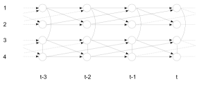
(a) TSC graph.

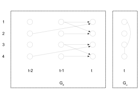
(b) GVAR structure.

Figure 1: (a) TSC graph and (b) corresponding GVAR structure of a sparse VAR(2) process.

To compactly encode $G_{TS}$, which essentially is a graph over all time steps, we will use the subgraphs $G_{d}\triangleq(V_{d},E_{d})$ and $G_{u}\triangleq(V_{u},E_{u})$. The temporal graph $G_{d}$, with respect to the reference time step $t$, contains the directed edges from the lagged node sets $V_{t-1},\ldots,V_{t-k}$ to $V_{t}$. The contemporaneous graph $G_{u}$ contains the undirected edges between the nodes in the same time step; $V_{u}=V_{t}$. Finally, following the graphical VAR modeling framework of [Epskamp-2018], we refer to the pair $G\triangleq(G_{d},G_{u})$ as a graphical VAR (GVAR) structure. For an example of a GVAR structure, see Figure 1(b).

2 Methods

The PLVAR method proposed in this paper utilizes a two-step approach for learning the GVAR model structure. Each step uses a score-based approach, where a candidate structure is scored according to how well it explains the dependence structure observed in the data. The proposed scoring function is based on a Bayesian framework for model selection. More specifically, PLVAR is based on the concept of objective Bayes factors for Gaussian graphical models, an approach that has been used successfully in the cross-sectional setting for learning the structure of decomposable undirected models [Carvalho-2009], directed acyclic graph (DAG) models [Consonni-2012], and general undirected models [Leppa-aho-2017]. More recently, this technique has also been used for learning the contemporaneous structure $G_{u}$ of a graphical VAR model under the assumption that the graph is chordal (decomposable) [Paci-2020]. By utilizing the Bayesian scoring function, we here develop an algorithm that infers the complete model structure $(G_{d},G_{u})$, where $G_{u}$ is allowed to be non-chordal. The method requires very little input from the user and is proven to be consistent in the large sample limit.

Given a scoring function, we still need an efficient search algorithm for finding the optimal structure. To enable scalability to high-dimensional systems, we propose a search algorithm that exploits the structure of the considered scoring function via a divide-and-conquer type approach. More specifically, the initial global structure learning problem is split up into multiple node-wise sub-problems whose solutions are combined into a final global structure. Since the number of possible structures in each sub-problem is still too vast for finding the global optimum for even moderate values of $d$ and $k$, a greedy search algorithm is used to find a local maximum in a reasonable time.

2.1 Bayesian model selection

The scoring function of the PLVAR method is derived using a Bayesian approach. Ideally, we are interested in finding a GVAR structure $G$ that is close to optimal in the sense of maximum a posteriori (MAP) estimation. By the Bayes’ rule,

$$p(G|\mathbf{Y})=\frac{p(\mathbf{Y}|G)p(G)}{\sum p(\mathbf{Y}|G)p(G)}$$ (9)

where $\mathbf{Y}\triangleq[\mathbf{y}_{1}\>\cdots\>\mathbf{y}_{N}]^{\top}$ is the observation matrix, and the sum in the denominator is taken over all the possible GVAR structures. Thus, the MAP estimate is given by

$$\hat{G}_{MAP}=\operatorname*{arg\,max\,}p(\mathbf{Y}|G)p(G).$$ (10)

A key part of of the above score is the marginal likelihood $p(\mathbf{Y}|G)$ which is obtained by integrating out the model parameters $\boldsymbol{\theta}$ in the likelihood $p(\mathbf{Y}|G,\boldsymbol{\theta})$ under some prior on the parameters.

Objective Bayesian model selection poses a problem in the specification of the parameter prior, as uninformative priors are typically improper. A solution to this is given by the fractional Bayes factor (FBF) approach [OHagan-1995], where a fraction of the likelihood is used for updating the improper uninformative prior into a proper fractional prior. The proper fractional prior is then used with the remaining part of likelihood to give the FBF. It has been shown that the FBF provides better robustness against misspecified priors compared to the use of proper priors in a situation where only vague information is available about the modeled system [OHagan-1995].

In this work, we make use of the objective FBF approach for Gaussian graphical models [Carvalho-2009, Consonni-2012, Leppa-aho-2017, Paci-2020]. In particular, our procedure is inspired by the fractional marginal pseudo-likelihood (FMPL) [Leppa-aho-2017], which allows for non-chordal undirected graphs when inferring the contemporaneous part of the network.

2.2 Fractional marginal pseudo-likelihood

In terms of Gaussian graphical models, the FBF was introduced for decomposable undirected models by [Carvalho-2009], and extended to DAG models by [Consonni-2012], who referred to the resulting score as the fractional marginal likelihood (FML). Finally, [Leppa-aho-2017] extended the applicability of the FBF approach to the general class of non-decomposable undirected models by combining it with the pseudo-likelihood approximation [Besag-1975]. Our procedure is inspired by the FMPL and can be thought of as an extension of the approach to time-series data.

As stated in [Leppa-aho-2017], the FMPL of a Gaussian graphical model is given by

$$pl(\mathbf{Y}|G) =\prod_{i=1}^{d}p(\mathbf{Y}_{i}|\mathbf{Y}_{\text{mb}(i)})$$ (11)

$$=\prod_{i=1}^{d}\pi^{-\frac{N-1}{2}}\frac{\Gamma\left(\frac{N+p_{i}}{2}\right)}{\Gamma\left(\frac{p_{i}+1}{2}\right)}N^{-\frac{2p_{i}+1}{2}}\left(\frac{\left|\mathbf{S_{\text{fa($i$)}}}\right|}{\left|\mathbf{S_{\text{mb($i$)}}}\right|}\right)^{-\frac{N-1}{2}},$$

where $\text{mb}(i)$ denotes the Markov blanket of $i$, $p_{i}$ denotes the number of nodes in $\text{mb}(i)$, and $\text{fa}(i)=\text{mb}(i)\cup i$ is the family of $i$. Moreover, $N$ denotes the number of observations, $\mathbf{S}=\mathbf{Y}^{\top}\mathbf{Y}$, and $\mathbf{S_{\text{fa($i$)}}}$ and $\mathbf{S_{\text{mb($i$)}}}$ denote the submatrices of $\mathbf{S}$ restricted to the nodes that belong to the family and Markov blanket, respectively, of node $i$. The FMPL is well-defined if $N-1\geq\max_{i}(p_{i})$, since it ensures (with probability one) positive definiteness of $\mathbf{S_{\text{fa($i$)}}}$ for each $i=1,\ldots,d$. Thus, we assume that this (rather reasonable) sparsity condition holds in the following.

Whereas [Leppa-aho-2017] is solely concerned with the learning of undirected Gaussian graphical models, we are interested in learning a GVAR structure which is made up of both a directed temporal part $G_{d}$ and an undirected contemporaneous part $G_{u}$. Rather than inferring these simultaneously, we break up the problem into two consecutive learning problems that both can be approached using the FMPL. First, in terms of $G_{d}$, we apply a modified version of (11) where the Markov blankets are built from nodes in earlier time steps. In terms of $G_{u}$, we use the inferred directed structure $\hat{G}_{d}$ to account for the temporal dependence between the observations. As this reduces the problem of inferring $G_{u}$ to the cross-sectional setting considered in [Leppa-aho-2017], the score in (11) can be applied as such.

2.3 Learning the temporal network structure

In order to learn the temporal part of the GVAR structure, we begin by creating a lagged data matrix

$$\mathbf{Z}\triangleq[\mathbf{Y}_{0}\>\mathbf{Y}_{-1}\>\cdots\>\mathbf{Y}_{-k}]$$ (12)

where $\mathbf{Y}_{-m}=[\mathbf{y}_{k-m+1}\>\cdots\>\mathbf{y}_{N-m}]^{\top}$. The lagged data matrix thus contains $(k+1)d$ columns, each corresponding to a time-specific variable; more specifically, the variable of the $m$:th time series at lag $l$ corresponds to column $ld+m$. As a result of the missing lag information in the beginning of the time-series, the effective number of observations (rows) is reduced from $N$ to $N-k$; this, however, poses no problems as long as $N$ is clearly larger than $k$.

Now, the problem of inferring the temporal structure can be thought of as follows. For each node $i$, we want to identify, among the lagged variables, a minimal set of nodes that will shield node $i$ from the remaining lagged variables, that is, a type of temporal Markov blanket. As seen in (7), the temporal Markov blanket will equal the set of lagged variables from which there is a directed edge to node $i$, commonly referred to as the parents of $i$. Assuming a structure prior that factorizes over the Markov blankets and a given lag length $k$, we can frame this problem as the following optimization problem based on the lagged data matrix and a modified version of (11):

$$\underset{\text{mb}(i)}{\arg\max}\ \ \ \prod_{i=1}^{d}p(\mathbf{Z}_{i}|\mathbf{Z}_{\text{mb}(i)},k)p(\text{mb}(i)|k)$$ (13)

$$\text{subject to }\ \ \text{mb}(i)\subseteq\{d+1,\ldots,(k+1)d\},$$

where the so-called local FMPL is here defined as

$$p(\mathbf{Z}_{i}|\mathbf{Z}_{\text{mb}(i)},k)\triangleq$$

$$\pi^{-\frac{N-k-1}{2}}\frac{\Gamma\left(\frac{N-k+p_{i}}{2}\right)}{\Gamma\left(\frac{p_{i}+1}{2}\right)}(N-k)^{-\frac{2p_{i}+1}{2}}\left(\frac{\left|\mathbf{S_{\text{fa($i$)}}}\right|}{\left|\mathbf{S_{\text{mb($i$)}}}\right|}\right)^{-\frac{N-k-1}{2}}.$$ (14)

The unscaled covariance matrix in (2.3) is now obtained from the lagged data matrix $\mathbf{Z}$, that is, $\mathbf{S}=\mathbf{Z}^{\top}\mathbf{Z}$.

The only thing left to specify in (13) is the structure prior. To further promote sparsity in the estimated network, we draw inspiration from the extended Bayesian information criterion (eBIC; see, for example, [Barber-2015]) and define our prior as

$$p(G_{d}|k)=\prod_{i=1}^{d}p(\text{mb}(i)|k)=\prod_{i=1}^{d}(kd)^{-\gamma p_{i}},$$ (15)

where $p_{i}$ is the number of nodes in the Markov blanket of node $i$ and $\gamma$ is a tuning parameter adjusting the strength of the sparsity promoting effect. As the default value for the tuning parameter, we use $\gamma=0.5$. As seen later, this prior will be essential for selecting the lag length.

From a computational point of view, problem (13) is very convenient in the sense that it is composed of $d$ separate sub-problems that can be solved independently of each other. To this end, we apply the same greedy search algorithm as in [Pensar-2017, Leppa-aho-2017].

2.4 Search algorithm

The PLVAR method uses a greedy search algorithm to find the set $\text{mb}(i)$ (with $p_{i}\leq N-1$) that maximizes the local FMPL for each $i\in V$. The search algorithm used by the PLVAR method has been published as Algorithm 1 in [Leppa-aho-2017] and originally introduced as Algorithm 1 in [Pensar-2017], based on [Tsamardinos-2006]. This algorithm works in two interleaving steps, deterministically adding and removing individual nodes in the set $\text{mb}(i)$. At each step, the node $j\notin\text{mb}(i)$ that yields the largest increase in the local FMPL is added to or removed from $\text{mb}(i)$. This is a hybrid approach aimed for low computational cost without losing much of the accuracy of an exhaustive search [Pensar-2017]. Pseudo-code for the algorithm is given in Appendix A.

2.5 Selecting the lag length

As noted in Subsection 2.3, the FMPL of a graphical VAR model depends on the lag length $k$. Unfortunately, the true value of $k$ is usually unknown in real-world problems. For the PLVAR method, we adopt the approach of setting an upper bound $K$ and learning the temporal structure separately for each $k=1,...,K$. The value of $K$ should preferably be based on knowledge about the problem domain, e.g. by considering the time difference between the observations and the maximum time a variable can influence itself or the other variables.

Once the upper bound $K$ has been set, a score is calculated for each $k$. Typical scores used for this purpose include the Bayesian information criterion and the Akaike information criterion, both of which are to be minimized. For the PLVAR method, we eliminate the need for external scores by selecting the $k$ that maximizes our FMPL-based objective function in (13). To ensure comparable data sets for different values on $k$, the time steps included in the lagged data matrices are determined by the maximum lag $K$. Note that our lag selection criterion is made possible by our choice of structure prior (15) which depends on $k$. As there is no restriction that a temporal Markov blanket should include nodes of all considered lags, the FMPL part of the objective function does not explicitly penalize overly long lag lengths.

2.6 Learning the contemporaneous network structure

Once the temporal network structure has been estimated, we proceed to learn the contemporaneous structure in three steps. First, the non-zero parameters of the lag matrices $\mathbf{A}_{m}$ are estimated via the ordinary least squares method (which is applicable under the sparsity condition $p_{i}\leq N-1$): this is done separately for each node given its temporal Markov blanket (or parents) in the temporal network. Next, the fully estimated lag matrices $\hat{\mathbf{A}}_{m}$ are used to calculate the residuals $\hat{\boldsymbol{\epsilon}}_{t}$ between the true and the predicted observations:

$$\hat{\boldsymbol{\epsilon}}_{t}=\mathbf{y}_{t}-\sum_{m=1}^{k}\hat{\mathbf{A}}_{m}\mathbf{y}_{t-m}.$$ (16)

If the estimates $\hat{\mathbf{A}}_{m}$ are accurate, the residuals $\hat{\boldsymbol{\epsilon}}_{t}$ will form a set of approximately cross-sectional data, generated by the contemporaneous part of the model, and the problem is reduced to the setting of the original FMPL method. Thus, as our objective function, we use the standard FMPL (11) in combination with our eBIC type prior:

$$p(G_{u})=\prod_{i=1}^{d}p(\text{mb}(i))=\prod_{i=1}^{d}(d-1)^{-\gamma p_{i}},$$ (17)

The only difference to (15) is the number of possible Markov blanket members which is now $d-1$. Again, as the default value for the tuning parameter, we use $\gamma=0.5$.

Although the Markov blankets are now connected through the symmetry constraint $i\in\text{mb}(j)\Leftrightarrow j\in\text{mb}(i),$ we use the same divide-and-conquer search approach as was used for the temporal part of the network. However, since the search may then result in asymmetries in the Markov blankets, we use the OR-criterion as described in [Leppa-aho-2017] when constructing the final graph: if $i\in\text{mb}(j)$ or $j\in\text{mb}(i)$, then $(i,j)\in E_{u}$.

2.7 Consistency of PLVAR

A particularly desirable characteristic for any statistical estimator is consistency. This naturally also applies when learning the GVAR structure. Importantly, it turns out that the proposed PLVAR method enjoys consistency. More specifically, as the sample size tends to infinity, PLVAR will recover the true GVAR structure, including the true lag length $k^{*}$, if the maximum considered lag length $K$ is larger than or equal to $k^{*}$. A brief outline of the rationale is provided in this subsection, and a formal proof of the key steps is provided in Appendix B.

The authors of [Leppa-aho-2017] show that their FMPL score in combination with the greedy search algorithm is consistent for finding the Markov blankets in Gaussian graphical models. Assuming a correct temporal structure, the lag matrices can be consistently estimated by the LS method [Lutkepohl-2005], and the residuals will thus tend towards i.i.d. samples from $N(\mathbf{0},\boldsymbol{\Sigma})$, where the sparsity pattern of $\Omega=\Sigma^{-1}$ corresponds to the contemporaneous structure. This is the setting considered in [Leppa-aho-2017], for which consistency has been proven.

What remains to be shown is that the first step of PLVAR is consistent in terms of recovering the temporal structure. Since PLVAR uses a variant of FMPL where the set $\text{mb}(i)$ is selected from lagged variables, it can be proven, using a similar approach as in [Leppa-aho-2017], that PLVAR will recover the true temporal Markov blankets (or parents) in the large sample limit if $K\geq k^{*}$ (see Appendix B for more details). Finally, since the structure prior (15) is designed to favor shorter lag lengths, it will in combination with the FMPL ensure that the estimated lag length will equal $k^{*}$ in the large sample limit.

As opposed to LASSO and SCAD, PLVAR needs no conditions on the measurement matrix and relation to true signal strength for model selection consistency [Zhao-2006, Buhlmann-2013, Huang-2007]. The reason for this lies in the difference between the approaches. In LASSO and SCAD, the regularization term introduces bias to the cost function, thereby deviating the estimation from the true signal [Zhao-2006, Buhlmann-2013]. On the other hand, PLVAR estimates the graph structure using the FMPL score: this is a Bayesian approach and thus has no bias in asymptotic behavior [Consonni-2012, Leppa-aho-2017].

2.8 Estimating the remaining parameters

Once the PLVAR method has been used to infer the model structure, the remaining parameters can be estimated as described in this subsection. This combination provides a complete pipeline for the learning of graphical VAR models.

The parameters that still remain unknown at this point are the non-zero elements of the lag matrices $\mathbf{A}_{m},m=1,\ldots,k$ and the non-zero elements of the precision matrix $\boldsymbol{\Omega}$. We calculate ML estimates for these parameters iteratively until a convergence criterion is met.

In each iteration, we first estimate the remaining elements of $\mathbf{A}_{m}$ given the current precision matrix. As initial value for the precision matrix, we use the identity matrix. In order to enforce the sparsity pattern implied by the temporal network, we use the ML estimation procedure described in [Lutkepohl-2005]. Next, we calculate the residuals between the true and predicted observations. We then estimate the remaining elements of $\boldsymbol{\Omega}$ from the residuals while enforcing the sparsity pattern learned earlier for the contemporaneous network: this is done by applying the ML estimation approach outlined in [Hastie-2009].

The iterations are repeated until the absolute difference between the current and the previous maximized log-likelihood of $\boldsymbol{\Omega}$ is smaller than a threshold $\delta$.

3 Experiments and results

In order to assess the performance of the PLVAR method, we made a number of experiments on both synthetic and real-world data. For the synthetic data, we used a single node in the Puhti supercomputer of CSC – IT Center for Science, Finland, equipped with 4 GB RAM and an Intel^® Xeon^® Gold 6230 processor with 20 physical cores at 2.10 GHz base frequency. For the real-world data, we used a laptop workstation equipped with 8 GB RAM and an Intel^® Core^™ i7-6700HQ CPU with 4 physical cores at 2.60 GHz base frequency. The algorithms were implemented in the R language. For the sparsity-constrained ML estimation of $\boldsymbol{\Omega}$, we used the implementation in the R package mixggm [Fop-2019]. The threshold $\delta$ for determining the convergence of the parameter estimation was set to $10^{-6}$.

3.1 Synthetic data

The performance of the PLVAR method was first evaluated in a controlled setting on data generated from known models with a ground truth structure. Having access to the true network structure, the quality of the inferred network structures were assessed by precision: the proportion of true edges among the inferred edges, and recall: the proportion of detected edges out of all true edges. Precision and recall were calculated separately for the temporal and the contemporaneous part of the network.

The R package SparseTSCGM [Abegaz-2013] was used to generate GVAR models with a random network structure and lag length $k=2$. We performed two experiments. In the first experiment, we fixed the degree of sparsity and varied the number of variables, $d\in\{20,40,80\}$. In the second experiment, we fixed the number of variables to $d=40$ and varied the degree of sparsity. The degree of sparsity in the generated networks is controlled by an edge inclusion probability parameter, called prob0. In order to have similar adjacency patterns for different number of variables, we specified the edge inclusion parameter as $q/(kd)$, meaning that the average indegree in the temporal structure is $q$ and the average number of neighbors in the contemporaneous structure is $q/2$. In the first experiment, we set $q=3$, resulting in rather sparse structures, and in the second experiment, we let $q\in\{5,7,9\}$, resulting in increasingly denser structures. For each considered configuration of $d$ and $q$, we generated 20 stable GVAR models. Finally, a single time series over 800 time points was generated from each model, and the $N$ first observations, with $N$ varying between 50 and 800, were used to form the final collection of data sets.

For comparison, LASSO and SCAD were also applied to the generated data, using the implementations available in SparseTSCGM. While LASSO and SCAD were given the correct lag length $k=2$, PLVAR was given a maximum allowed lag length $K=5$ and thereby tasked with the additional challenge of estimating the correct lag length. In terms of the tuning parameters, the $\gamma$ prior parameter in PLVAR was set to 0.5, and the remaining parameters of LASSO and SCAD were set according to the example provided in the SparseTSCGM manual. More specifically, the maximum number of outer and inner loop iterations were set to 10 and 100, respectively. The default grid of candidate values for the tuning parameters (lam1 and lam2) were used, and the optimal values were selected using the modified Bayesian information criterion (bic_mod).

The precision, recall and running times of the considered methods are summarized in Figure 2 for the first experiment and in Figure 3 for the second experiment. For some of the most challenging settings: $N=50$ for $d\in\{40,80\}$ and $N=100$ for $d=80$, LASSO and SCAD exited with an error and the results are therefore missing. In terms of precision (Figures 2(a) and 3(a)), PLVAR is clearly the most accurate of the methods, both for the temporal and the contemporaneous part of the network structure. In terms of recall (Figures 2(b) and 3(b)), all methods perform very well for the larger samples, recovering close to all edges. For smaller sample sizes, PLVAR has a slight edge on both LASSO and SCAD in the sparser settings, $q=3$ and $q=5$, while it is overall quite even in the denser setting $q=7$, and the situation is almost reversed for $q=9$.

As expected, increasing the number of variables or the number of edges makes the learning problem harder, leading to a reduced accuracy. However, there is no drastic reduction in accuracy for any of the methods. The most drastic change between the settings is perhaps the computation time of LASSO and SCAD when the number of variables is increased (Figure 2(c)). Overall, PLVAR was orders of magnitude faster than LASSO and SCAD, both of which use cross-validation to select the regularization parameters. However, it must be noted that PLVAR solves a simpler problem in that it focuses on learning the model structure (yet without a given lag length), while the likelihood-based methods also estimate the model parameters along with the structure. Still, the problem of estimating the model (parameters) is greatly facilitated once the model structure has been inferred.

Finally, when it comes to selecting the correct lag length ($k=2$) from the candidate lag lengths, PLVAR was highly accurate and estimated the lag length to be higher than 2 for only a few cases in both the sparse and the denser settings (Figure 4). It is also worth noting that while the maximum lag length supported by the PLVAR method is only limited by the available computing resources, the LASSO and SCAD implementations in SparseTSCGM currently only support lag lengths 1 and 2.

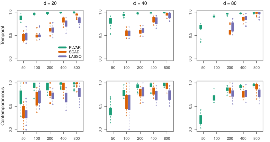
(a) Precision.

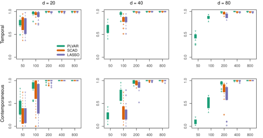
(b) Recall.

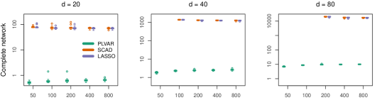
(c) Computation time.

Figure 2: Results of the simulation study with a fixed degree of sparsity ($q=3$) and an increasing number of variables: (a) Precision and (b) recall (y-axis) for the temporal and contemporaneous part of the network structure for various sample sizes (x-axis) and model size, $d$. (c) Recorded computation times (y-axis in log scale) for learning the complete network structure. Part of the results are missing for LASSO and SCAD since they exited with an error for some of the settings. The statistics shown in the plots have been calculated from a sample of 20 random GVAR models.

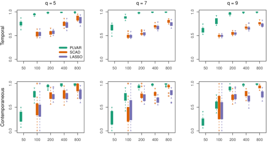
(a) Precision.

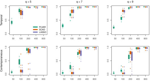
(b) Recall.

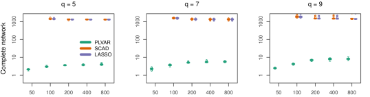
(c) Computation time.

Figure 3: Results of the simulation study with a fixed number of variables ($d=40$) and a decreasing degree of sparsity: (a) Precision and (b) recall (y-axis) for the temporal and contemporaneous part of the network structure for various sample sizes (x-axis) and degrees of sparsity, as controlled by $q$. (c) Recorded computation times (y-axis in log scale) for learning the complete network structure. Part of the results are missing for LASSO and SCAD since they exited with an error when $N=50$. The statistics shown in the plots have been calculated from a sample of 20 random GVAR models.

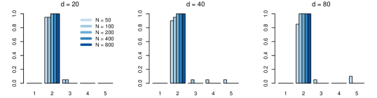
(a)

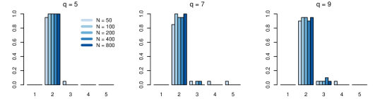
(b)

Figure 4: Estimated lag length by PLVAR for the different sample sizes in the simulation studies: (a) $q=3$ and (b) $d=40$. The x-axis represents the candidate lag lengths and the y-axis represents the percentage of times a specific lag length was chosen. The correct lag length is 2 in all cases.

3.2 Electroencephalography data

Since VAR models have found extensive use in EEG analysis, the experiments made on synthetic data were complemented with experiments on real-world EEG data. The dataset chosen for this purpose is a subset of the publicly available CHB-MIT Scalp EEG Database (CHBMIT) [Shoeb-2009, Goldberger-2000].

The CHBMIT database contains a total of 24 cases of EEG recordings, collected from 23 pediatric subjects at the Children’s Hospital Boston. Each case comprises multiple recordings stored in European Data Format (.EDF) files. However, only the first recording of each unique subject was used in order to speed up the experiments. Case 24 was excluded since it has been added afterwards and is missing gender and age information. The recordings included in the experiments are listed in Table 1.

Table 1: Recordings included in the EEG experiments

recording filename	subject gender	subject age (years)
chb01_01.edf	female	11
chb02_01.edf	male	11
chb03_01.edf	female	14
chb04_01.edf	male	22
chb05_01.edf	female	7
chb06_01.edf	female	1.5
chb07_01.edf	female	14.5
chb08_02.edf	male	3.5
chb09_01.edf	female	10
chb10_01.edf	male	3
chb11_01.edf	female	12
chb12_06.edf	female	2
chb13_02.edf	female	3
chb14_01.edf	female	9
chb15_02.edf	male	16
chb16_01.edf	female	7
chb17a_03.edf	female	12
chb18_02.edf	female	18
chb19_02.edf	female	19
chb20_01.edf	female	6
chb22_01.edf	female	9
chb23_06.edf	female	6

The recordings in the CHBMIT database have been collected using the international 10-20 system for the electrode placements. The channels derived from the electrodes vary between files and some channels only exist in a subset of the recordings. Hence, the experiments were made using only those 21 channels that can be found in all the recordings, implying $d=21$ in the VAR models. Table 2 lists the channels included in the experiments.

Table 2: Channels included in the EEG experiments

FP1-F7	F7-T7	T7-P7	P7-O1
FP1-F3	F3-C3	C3-P3	P3-O1
FP2-F4	F4-C4	C4-P4	P4-O2
FZ-CZ	CZ-PZ	T7-FT9
FT9-FT10	FT10-T8

All the recordings have a sampling rate of 256 Hz. The first 60 seconds were skipped in each recording because the signal-to-noise ratio in the beginning of some recordings is very low. The next 256 samples were used as training data and presented to each method for learning the model structure and the model parameters. The following 512 samples were used as test data to evaluate the performance of the methods.

Each experiment was made using 6 different algorithms. In addition to PLVAR, LASSO, and SCAD, conventional LS estimation was included for comparison. As noted before, the SparseTSCGM implementations of LASSO and SCAD only allow lag lengths 1 and 2. Therefore, the final set of algorithms comprised PLVAR, LS, PLVAR2, LS2, LASSO2, and SCAD2. In this set, algorithm names ending with 2 refer to the respective methods provided with lag length 2 for straightforward comparison. The names PLVAR and LS refer to respective methods with no a priori lag length information.

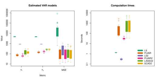
Figure 5: Results on EEG data. $n_{\text{t}}$, $n_{\text{c}}$, and MSE denote the number of edges in the temporal network, the number of edges in the contemporaneous network, and the mean squared error of 1-step predictions on the test data, respectively. Note the logarithmic $y$ axis in both subplots.

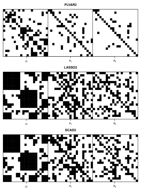
Figure 6: Adjacency matrix estimates, obtained from the EEG recording chb06_01.edf using the PLVAR2, the LASSO2, and the SCAD2 methods. The black and white pixels correspond to non-zero and zero elements in the matrices, respectively. $\boldsymbol{\Omega}$ refers to the precision matrix, $\mathbf{A}_{1}$ to the first lag matrix, and $\mathbf{A}_{2}$ to the second lag matrix. Note the sparsity of the PLVAR2 estimates as compared to the other methods.

The performance of each algorithm was evaluated using the following metrics: the number of edges in the estimated temporal network ($n_{\text{t}}$), the number of edges in the estimated contemporaneous network ($n_{\text{c}}$), the mean squared error (MSE) of 1-step predictions on the test data, and the estimation time in seconds ($t$). The results are summarized in Figure 5. An example of the estimated temporal and contemporaneous networks is given in Figure 6 where the networks are visualized through their adjacency matrices.

Figure 5 shows that PLVAR and PLVAR2 produced the sparsest estimates for both the temporal network and the contemporaneous network. The dense estimates produced by LS and LS2 had an order of magnitude more edges than the estimates obtained through PLVAR and PLVAR2. The difference between the likelihood-based methods and the PLVAR methods is smaller but still evident. The MSEs on the test data were somewhat equal for all the methods except for LS and LS2. The MSEs obtained through LS2 were slightly higher that the MSEs obtained through the likelihood-based and the PLVAR methods. The MSEs produced by LS were about 100 times as high.

The computation times were minimal for LS and LS2 but this makes hardly a difference if the goal is to learn a sparse VAR model. The computation time required by PLVAR2 was an order of magnitude shorter than the time required by LASSO2 and SCAD2. The PLVAR method, tasked with the additional challenge of estimating the lag length, was slower than PLVAR2 but still faster than LASSO2 and SCAD2.

The example in Figure 6 highlights the difference in sparsity of the model estimates obtained through PLVAR2 and the likelihood-based methods. In this particular case, it is evident that PLVAR2 produced the sparsest precision matrix and lag matrices, corresponding to the contemporaneous network and temporal network, respectively. One can find some common structures in all the precision matrices but the structures in the likelihood-based estimates are much denser.

4 Discussion

In this paper we have extended the idea of structure learning of Gaussian graphical models via pseudo-likelihood and Bayes factors from the cross-sectional domain into the time-series domain of VAR models. We have presented a novel method, PLVAR, that is able to infer the complete VAR model structure, including the lag length, in a single run. We have shown that the PLVAR method produces a consistent structure estimator in the class of VAR models. We have also presented an iterative maximum likelihood procedure for inferring the model parameters for a given sparse VAR structure, providing a complete VAR model learning pipeline.

The experimental results on synthetic data suggest that the PLVAR method is better suited for recovering sparse VAR structures than the available likelihood-based methods, a result that is in line with previous research [Leppa-aho-2017, Pensar-2017]. The results on EEG data provide further evidence on the feasibility of the PLVAR method. Even though LASSO and SCAD reached quite similar MSEs, PLVAR was able to do so while producing much sparser models and using significantly less computation time. The conventional LS and LS2 methods were even faster but they are unable to learn sparse VAR models. Also, the MSEs produced by LS and LS2 were the highest among all the methods under consideration. All in all, the results show that PLVAR is a highly competitive method for high-dimensional VAR structure learning, from both an accuracy point of view and a purely computational point of view.

It should be noted that the PLVAR implementation used in the experiments is purely sequential. It would be relatively straightforward to make the search algorithm run in parallel, thereby reducing the computation time up to $1/n_{\text{cpus}}$ where $n_{\text{cpus}}$ is the number of CPU cores available on the system. While it is common for modern desktop and laptop workstations to be equipped with 4 to 8 physical cores, parallelization can be taken much further by utilizing cloud computing services. Several cloud vendors offer high-power virtual machines with tens of CPUs and the possibility of organizing them into computing clusters. This makes PLVAR highly competitive against methods that cannot be easily parallelized, especially when the number of variables in the model is large.

In summary, PLVAR is an accurate and fast method for learning VAR models. It is able to produce sparse estimates of the model structure and thereby allows the model to be interpreted to gain additional knowledge in the problem domain.

In future work, we plan to apply the PLVAR method to domains that make extensive use of VAR modeling and where improvements in estimation accuracy and speed have the potential to enhance the end results significantly. An example of these domains is brain research where brain connectivity is measured in terms of Granger causality index, directed transfer function, and partial directed coherence. Since these measures are derived from VAR models estimated from the data, one can expect more accurate estimates to result in more accurate measures of connectivity. Moreover, the enhanced possibilites in VAR model fitting introduced here allow more complex models to be studied. Further research with applications to other high-dimensional problems is also encouraged.

Supplementary material

The R code written for the experiments is publicly available in the repository https://github.com/kimmo-suotsalo/plvar. The EEG data can be freely obtained from PhysioNet [Goldberger-2000] at https://www.physionet.org/content/chbmit/1.0.0/.

Appendices

A Pseudo-code for the search algorithm

The pseudo-code for the greedy search procedure is presented in Algorithm 1. The algorithm has been published previously in [Leppa-aho-2017] and was originally introduced in [Pensar-2017], based on [Tsamardinos-2006].

Algorithm 1 Greedy search for finding the temporal Markov blanket of node $i$

1:function find_mb($i,\mathbf{Z},k$)

2:     mb($i$), $\widehat{\text{mb}}$($i$) $\leftarrow\emptyset$

3:     while $\widehat{\text{mb}}$($i$) has changed AND $|\text{mb}(i)|<N-1$  do

4:         C $\leftarrow V\setminus\text{fa}(i)$

5:         $\triangleright$ above, $V$ contains lagged variables from $t-1$ to $t-k$

6:         mb($i$) $\leftarrow\widehat{\text{mb}}(i)$

7:         for $j\in C$ do

8:              if $p(\mathbf{Z}_{i}|\mathbf{Z}_{\text{mb}(i)\cup\{j\}},k)$ $>$ $p(\mathbf{Z}_{i}|\mathbf{Z}_{\widehat{\text{mb}}(i)},k)$ then

9:                  $\widehat{\text{mb}}$($i$) $\leftarrow$ mb($i$) $\cup\{j\}$

10:              end if

11:         end for

12:         while $\widehat{\text{mb}}$($i$) has changed do

13:              mb($i$) $\leftarrow\widehat{\text{mb}}(i)$

14:              for $j\in\text{mb}(i)$ do

15:                  if $p(\mathbf{Z}_{i}|\mathbf{Z}_{\text{mb}(i)\setminus\{j\}},k)$ $>$ $p(\mathbf{Z}_{i}|\mathbf{Z}_{\widehat{\text{mb}}(i)},k)$ then

16:                       $\widehat{\text{mb}}$($i$) $\leftarrow$ mb($i$) $\setminus\{j\}$

17:                  end if

18:              end for

19:         end while

20:     end while

21:     return $\widehat{\text{mb}}(i)$

22:end function

B Consistency proof

The below result states that the modified FMPL given in (13) is consistent for inferring the temporal Markov blankets in the considered model class. The proof is adapted from [Leppa-aho-2017] where the authors use a similar reasoning for Gaussian graphical models with cross-sectional data.

Theorem 1.

Define $\mathbf{Z}$ and $p(\mathbf{Z}_{i}|\mathbf{Z}_{\text{mb}(i)},k)$ as in Equation (12) and (2.3), respectively. Let $S=\{d+1,\ldots,(k+1)d\}$ contain the true temporal Markov blanket $\text{mb}(i)^{*}$ or, equivalently, let $k\geq k^{*}$ where $k^{*}$ is the true lag length. Then,

$$\operatorname*{plim\,}_{N\rightarrow\infty}\operatorname*{arg\,max\,}_{\text{mb}(i)\subseteq S}p(\mathbf{Z}_{i}|\mathbf{Z}_{\text{mb}(i)},k)=\text{mb}(i)^{*}.$$ (18)

Proof.

Under the current assumption of i.i.d. $N(\mathbf{0},\Sigma)$ error terms, it can be shown that $\mathbf{y}_{t}$ is a Gaussian process, meaning that the subcollections $\mathbf{y}_{t},\mathbf{y}_{t-1},\ldots,\mathbf{y}_{t-k}$ have a multivariate normal distribution [Lutkepohl-2005]. Thus, $\mathbf{Z}$ can be considered a data matrix generated from a multivariate normal distribution over the variables $Z_{1},\ldots,Z_{(k+1)d}$ where the dependence structure of the model is determined by the GVAR structure. In particular, following from the directed Markov property in (7), the dependence structure will be such that

$$Z_{i}\perp Z_{\text{mb}(i)^{*}}\mid Z_{S\setminus\text{mb}(i)^{*}},$$

where $i\in\{1,\ldots,d\}$. Following a similar line of reasoning as in [Leppa-aho-2017], we can now show through Lemma 1 and Lemma 2 that (18) holds. More specifically, Lemma 1 guarantees that as $N\rightarrow\infty$,

$$p(\mathbf{Z}_{i}|\mathbf{Z}_{\text{mb}(i)},k)<p(\mathbf{Z}_{i}|\mathbf{Z}_{\text{mb}(i)^{*}},k)$$

for any $\text{mb}(i)$ that does not contain all the nodes in $\text{mb}(i)^{*}$. Similarly, Lemma 2 guarantees that as $N\rightarrow\infty$,

$$p(\mathbf{Z}_{i}|\mathbf{Z}_{\text{mb}(i)},k)<p(\mathbf{Z}_{i}|\mathbf{Z}_{\text{mb}(i)^{*}},k)$$

for any $\text{mb}(i)$ that contains one or more nodes not in $\text{mb}(i)^{*}$. ∎

The proofs of Lemma 1 and Lemma 2 follow closely those of [Leppa-aho-2017]. However, for completeness, we give here the proofs in detail.

Lemma 1.

Let $\text{mb}(i)\subset\text{mb}(i)^{*}$ and $A\subset V\setminus\text{fa}(i)^{*}$. Then

$$\operatorname*{plim\,}_{N\rightarrow\infty}\log\frac{p(\mathbf{Z}_{i}|\mathbf{Z}_{\text{mb}(i)^{*}\cup A},k)}{p(\mathbf{Z}_{i}|\mathbf{Z}_{\text{mb}(i)\cup A},k)}=\infty.$$ (19)

Proof.

By defining $p_{i}\triangleq|\text{mb}(i)^{*}\cup A|$ and $a\triangleq|\text{mb}(i)\cup A|-p_{i}$, we have that

$$\log\frac{p(\mathbf{Z}_{i}|\mathbf{Z}_{\text{mb}(i)^{*}\cup A},k)}{p(\mathbf{Z}_{i}|\mathbf{Z}_{\text{mb}(i)\cup A},k)}=\log\frac{\Gamma\left(\frac{N-k+p_{i}}{2}\right)}{\Gamma\left(\frac{N-k+p_{i}+a}{2}\right)}+$$

$$\log\frac{\Gamma\left(\frac{p_{i}+a+1}{2}\right)}{\Gamma\left(\frac{p_{i}+1}{2}\right)}+a\log(N-k)-$$

$$\frac{N-k-1}{2}\log\frac{\left|\mathbf{S_{\text{fa($i$)${}^{*}\cup A$}}}\right|\left|\mathbf{S_{\text{mb($i$)$\cup A$}}}\right|}{\left|\mathbf{S_{\text{mb($i$)${}^{*}\cup A$}}}\right|\left|\mathbf{S_{\text{fa($i$)$\cup A$}}}\right|}.$$ (20)

The first term on the right-hand side equals

$$\log\Gamma(M)-\log\Gamma\left(M+\frac{a}{2}\right)$$ (21)

where $M=(N-k+p_{i})/2$. As $N\rightarrow\infty$, $M\rightarrow\infty$ and by Stirlings’s formula

$$\log\Gamma(M)-\log\Gamma\left(M+\frac{a}{2}\right)=\left(M-\frac{1}{2}\right)\log M-M$$

$$-\left[\left(M+\frac{a}{2}-\frac{1}{2}\right)\log\left(M+\frac{a}{2}\right)-\left(M+\frac{a}{2}\right)\right]+O(1).$$ (22)

Here, the right-hand side can be written as

$$M\log\frac{M}{M+\frac{a}{2}}+\frac{1}{2}\log\frac{M+\frac{a}{2}}{M}-\frac{a}{2}\log\left(M+\frac{a}{2}\right)+O(1)$$ (23)

where we have included the term $a/2$ in $O(1)$. Since

$$M\log\frac{M}{M+\frac{a}{2}}=\frac{1}{2}\log\left(\frac{1}{1+\frac{a}{2M}}\right)^{2M}\xrightarrow[M\rightarrow\infty]{}$$

$$\frac{1}{2}\log e^{-a}=-\frac{a}{2}=O(1)$$ (24)

and

$$\frac{1}{2}\log\frac{M+\frac{a}{2}}{M}=\frac{1}{2}\log\left(1+\frac{a}{2M}\right)\xrightarrow[M\rightarrow\infty]{}0,$$ (25)

we have that

$$\log\frac{\Gamma\left(\frac{N-k+p_{i}}{2}\right)}{\Gamma\left(\frac{N-k+p_{i}+a}{2}\right)}\xrightarrow[N\rightarrow\infty]{}-\frac{a}{2}\log\left(\frac{N-k+p_{i}+a}{2}\right)+O(1).$$ (26)

The second term on the right-hand side of Equation (Proof.) can be included in $O(1)$ since it is constant with respect to $N$. The fourth term

$$-\frac{N-k-1}{2}\log\frac{\left|\mathbf{S_{\text{fa($i$)${}^{*}\cup A$}}}\right|\left|\mathbf{S_{\text{mb($i$)$\cup A$}}}\right|}{\left|\mathbf{S_{\text{mb($i$)${}^{*}\cup A$}}}\right|\left|\mathbf{S_{\text{fa($i$)$\cup A$}}}\right|}$$ (27)

can be expressed using the covariance $\boldsymbol{\Sigma}$: since $\mathbf{S}=\mathbf{Z}^{\top}\mathbf{Z}=N\widehat{\boldsymbol{\Sigma}}_{\text{ML}}$, it holds that

$$\frac{\left|\mathbf{S_{\text{fa($i$)${}^{*}\cup A$}}}\right|\left|\mathbf{S_{\text{mb($i$)$\cup A$}}}\right|}{\left|\mathbf{S_{\text{mb($i$)${}^{*}\cup A$}}}\right|\left|\mathbf{S_{\text{fa($i$)$\cup A$}}}\right|}\xrightarrow[N\rightarrow\infty]{}\frac{\left|\boldsymbol{\Sigma_{\text{fa($i$)${}^{*}\cup A$}}}\right|\left|\boldsymbol{\Sigma_{\text{mb($i$)$\cup A$}}}\right|}{\left|\boldsymbol{\Sigma_{\text{mb($i$)${}^{*}\cup A$}}}\right|\left|\boldsymbol{\Sigma_{\text{fa($i$)$\cup A$}}}\right|}$$ (28)

in probability. Let us now partition $\boldsymbol{\Sigma_{\text{fa($i$)${}^{*}\cup A$}}}$ as

$$\boldsymbol{\Sigma_{\text{fa($i$)${}^{*}\cup A$}}}=\begin{bmatrix}\sigma^{2}(z_{i})&\sigma(z_{i},\mathbf{z}_{\text{mb($i$)${}^{*}\cup A$}})\\ \sigma(z_{i},\mathbf{z}_{\text{mb($i$)${}^{*}\cup A$}})^{\top}&\boldsymbol{\Sigma}_{\text{mb($i$)${}^{*}\cup A$}}\end{bmatrix}$$ (29)

where $\sigma(z_{i},\mathbf{z}_{\text{mb($i$)${}^{*}\cup A$}})$ denotes a row vector whose elements are the covariances between the variable $z_{i}$ and each of the variables in mb($i$)${}^{*}\cup A$. The determinant of this partitioned matrix is

$$\left|\boldsymbol{\Sigma}_{\text{mb($i$)${}^{*}\cup A$}}\right|\cdot$$

$$\left[\sigma^{2}(z_{i})-\sigma(z_{i},\mathbf{z}_{\text{mb($i$)${}^{*}\cup A$}})\left(\boldsymbol{\Sigma}_{\text{mb($i$)${}^{*}\cup A$}}\right)^{-1}\sigma(z_{i},\mathbf{z}_{\text{mb($i$)${}^{*}\cup A$}})^{\top}\right]$$ (30)

where the term

$$\sigma(z_{i},\mathbf{z}_{\text{mb($i$)${}^{*}\cup A$}})\left(\boldsymbol{\Sigma}_{\text{mb($i$)${}^{*}\cup A$}}\right)^{-1}\sigma(z_{i},\mathbf{z}_{\text{mb($i$)${}^{*}\cup A$}})^{\top}\triangleq$$

$$\sigma(\hat{z}_{i}[\mathbf{z}_{\text{mb($i$)${}^{*}\cup A$}}])$$ (31)

is the variance of the linear LS predictor of $z_{i}$ from $\mathbf{z}_{\text{mb($i$)${}^{*}\cup A$}}$. By definition, the residual variance of $z_{i}$ after subtracting the variance of the linear LS predictor is the partial variance $\sigma(z_{i}|\mathbf{z}_{\text{mb($i$)${}^{*}\cup A$}})$; hence,

$$\left|\boldsymbol{\Sigma}_{\text{fa($i$)${}^{*}\cup A$}}\right|=\left|\boldsymbol{\Sigma}_{\text{mb($i$)${}^{*}\cup A$}}\right|\sigma(z_{i}|\mathbf{z}_{\text{mb($i$)${}^{*}\cup A$}})$$ (32)

which implies that

$$\frac{\left|\boldsymbol{\Sigma_{\text{fa($i$)${}^{*}\cup A$}}}\right|\left|\boldsymbol{\Sigma_{\text{mb($i$)$\cup A$}}}\right|}{\left|\boldsymbol{\Sigma_{\text{mb($i$)${}^{*}\cup A$}}}\right|\left|\boldsymbol{\Sigma_{\text{fa($i$)$\cup A$}}}\right|}=\frac{\sigma(z_{i}|\mathbf{z}_{\text{mb($i$)${}^{*}\cup A$}})}{\sigma(z_{i}|\mathbf{z}_{\text{mb($i$)$\cup A$}})}.$$ (33)

Combining the results so far, Equation (Proof.) can be rewritten as

$$\log\frac{p(\mathbf{Z}_{i}|\mathbf{Z}_{\text{mb}(i)^{*}\cup A},k)}{p(\mathbf{Z}_{i}|\mathbf{Z}_{\text{mb}(i)\cup A},k)}=-\frac{a}{2}\log\left(\frac{N-k+p_{i}+a}{2}\right)+$$

$$a\log(N-k)-\frac{N-k-1}{2}\log\frac{\sigma(z_{i}|\mathbf{z}_{\text{mb($i$)${}^{*}\cup A$}})}{\sigma(z_{i}|\mathbf{z}_{\text{mb($i$)$\cup A$}})}+O(1).$$ (34)

The second term on the right hand side equals

$$\frac{a}{2}\log(N-k)^{2}=\frac{a}{2}\log(N-k)+\frac{a}{2}\log(N-k)$$ (35)

and therefore

$$\log\frac{p(\mathbf{Z}_{i}|\mathbf{Z}_{\text{mb}(i)^{*}\cup A},k)}{p(\mathbf{Z}_{i}|\mathbf{Z}_{\text{mb}(i)\cup A},k)}=$$

$$\frac{a}{2}\log(N-k)-\frac{N}{2}\log\frac{\sigma(z_{i}|\mathbf{z}_{\text{mb($i$)${}^{*}\cup A$}})}{\sigma(z_{i}|\mathbf{z}_{\text{mb($i$)$\cup A$}})}+O(1).$$ (36)

Now, consider the argument of the last logarithm term. Assume first that $\text{mb($i$)}\neq\emptyset$ and let $B\triangleq\text{mb($i$)}^{*}\setminus\text{mb($i$)}$. Then

$$\sigma(\hat{z}_{i}[\mathbf{z}_{\text{mb($i$)${}^{*}\cup A$}}])=\sigma(\hat{z}_{i}[\mathbf{z}_{\text{mb($i$)$\cup A\cup B$}}])=$$

$$\sigma(\hat{z}_{i}[\mathbf{z}_{\text{mb($i$)$\cup A$}}])+\sigma(\hat{z}_{i}[\mathbf{z}_{B}-\hat{\mathbf{z}}_{B}[\mathbf{z}_{\text{mb($i$)$\cup A$}}]])$$ (37)

where the last term $\sigma(\hat{z}_{i}[\mathbf{z}_{B}-\hat{\mathbf{z}}_{B}[\mathbf{z}_{\text{mb($i$)$\cup A$}}]])>0$ since $B\subset\text{mb($i$)}^{*}$. Hence,

$$\sigma(\hat{z}_{i}[\mathbf{z}_{\text{mb($i$)${}^{*}\cup A$}}])>\sigma(\hat{z}_{i}[\mathbf{z}_{\text{mb($i$)$\cup A$}}])$$ (38)

which is equivalent to

$$\sigma^{2}(z_{i})-\sigma(\hat{z}_{i}[\mathbf{z}_{\text{mb($i$)${}^{*}\cup A$}}])<\sigma^{2}(z_{i})-\sigma(\hat{z}_{i}[\mathbf{z}_{\text{mb($i$)$\cup A$}}]).$$ (39)

This implies that

$$\sigma(z_{i}|\mathbf{z}_{\text{mb($i$)${}^{*}\cup A$}})<\sigma(z_{i}|\mathbf{z}_{\text{mb($i$)$\cup A$}})$$ (40)

and therefore the last logarithm term

$$-\frac{N}{2}\log\frac{\sigma(z_{i}|\mathbf{z}_{\text{mb($i$)${}^{*}\cup A$}})}{\sigma(z_{i}|\mathbf{z}_{\text{mb($i$)$\cup A$}})}\xrightarrow[N\rightarrow\infty]{}\infty.$$ (41)

Assume then that $\text{mb($i$)}=\emptyset$. This implies that

$$\sigma(\hat{z}_{i}[\mathbf{z}_{A}])+\sigma(\hat{z}_{i}[\mathbf{z}_{\text{mb($i$)${}^{*}$}}-\hat{z}_{\text{mb($i$)${}^{*}$}}[\mathbf{z}_{A}]])>\sigma(\hat{z}_{i}[\mathbf{z}_{A}])$$ (42)

which is equivalent to

$$\sigma(\hat{z}_{i}[\mathbf{z}_{\text{mb($i$)${}^{*}\cup A$}}])>\sigma(\hat{z}_{i}[\mathbf{z}_{A}])$$ (43)

and further to Inequation (38). Hence, the last logarithm term behaves exactly as for $\text{mb($i$)}\neq\emptyset$.

Since $\text{mb}(i)\subset\text{mb}(i)^{*}$, $a<0$, and the second-last logarithm term

$$\frac{a}{2}\log(N-k)\xrightarrow[N\rightarrow\infty]{}-\infty.$$ (44)

Combining all the results, we have that

$$\log\frac{p(\mathbf{Z}_{i}|\mathbf{Z}_{\text{mb}(i)^{*}\cup A},k)}{p(\mathbf{Z}_{i}|\mathbf{Z}_{\text{mb}(i)\cup A},k)}=$$

$$\frac{a}{2}\log(N-k)-\frac{N}{2}\log\frac{\sigma(z_{i}|\mathbf{z}_{\text{mb($i$)${}^{*}\cup A$}})}{\sigma(z_{i}|\mathbf{z}_{\text{mb($i$)$\cup A$}})}+O(1)$$ (45)

where the first and the second term on the right-hand side tend to $-\infty$ and $\infty$, respectively. However, since $-\log N$ decreases slower than $N$ increases, the right-hand side of the equation tends to $\infty$. This proves the statement of Lemma 1. ∎

Lemma 2.

Let $\text{mb}(i)^{*}\subset\text{mb}(i)$. Then

$$\operatorname*{plim\,}_{N\rightarrow\infty}\log\frac{p(\mathbf{Z}_{i}|\mathbf{Z}_{\text{mb}(i)^{*}},k)}{p(\mathbf{Z}_{i}|\mathbf{Z}_{\text{mb}(i)},k)}=\infty.$$ (46)

Proof.

By defining $p_{i}\triangleq|\text{mb}(i)^{*}|$ and $a\triangleq|\text{mb}(i)|-p_{i}$, we have that

Thisequationisidenticalto(

Proof.)exceptforthelasttermontheright-handside.AsN→∞,this