Convergence of Graph Laplacian with kNN Self-tuned Kernels

Abstract

Kernelized Gram matrix $W$ constructed from data points $\{x_{i}\}_{i=1}^{N}$ as $W_{ij}=k_{0}(\frac{\|x_{i}-x_{j}\|^{2}}{\sigma^{2}})$ is widely used in graph-based geometric data analysis and unsupervised learning. An important question is how to choose the kernel bandwidth $\sigma$, and a common practice called self-tuned kernel adaptively sets a $\sigma_{i}$ at each point $x_{i}$ by the $k$-nearest neighbor (kNN) distance. When $x_{i}$’s are sampled from a $d$-dimensional manifold embedded in a possibly high-dimensional space, unlike with fixed-bandwidth kernels, theoretical results of graph Laplacian convergence with self-tuned kernels have been incomplete. This paper proves the convergence of graph Laplacian operator $L_{N}$ to manifold (weighted-)Laplacian for a new family of kNN self-tuned kernels $W^{(\alpha)}_{ij}=k_{0}(\frac{\|x_{i}-x_{j}\|^{2}}{\epsilon\hat{\rho}(x_{i})\hat{\rho}(x_{j})})/\hat{\rho}(x_{i})^{\alpha}\hat{\rho}(x_{j})^{\alpha}$, where $\hat{\rho}$ is the estimated bandwidth function by kNN, and the limiting operator is also parametrized by $\alpha$. When $\alpha=1$, the limiting operator is the weighted manifold Laplacian $\Delta_{p}$. Specifically, we prove the point-wise convergence of $L_{N}f$ and convergence of the graph Dirichlet form with rates. Our analysis is based on first establishing a $C^{0}$ consistency for $\hat{\rho}$ which bounds the relative estimation error $|\hat{\rho}-\bar{\rho}|/\bar{\rho}$ uniformly with high probability, where $\bar{\rho}=p^{-1/d}$, and $p$ is the data density function. Our theoretical results reveal the advantage of self-tuned kernel over fixed-bandwidth kernel via smaller variance error in low-density regions. In the algorithm, no prior knowledge of $d$ or data density is needed. The theoretical results are supported by numerical experiments on simulated data and hand-written digit image data.

1 Introduction

Kernelized Gram matrix computed from data vectors $\{x_{i}\}_{i=1}^{N}$ in $\mathbb{R}^{D}$ has been a pivotal tool in kernel methods [40], graph-based manifold learning and geometric data analysis [2, 3, 13, 12, 52, 47], and semi-supervised learning [37, 46, 25, 26], among others. Applications range broadly from model reduction of chemical systems [44, 39, 48, 14] to general data visualization [8, 24, 30, 55]. The graph affinity matrix $W$, which is real symmetric and has non-negative entries, can be viewed as weights on the edges of a weighted undirected graph, denoted as ${\cal G}=(V,E)$, $V=\{1,\cdots,N\}$, and $E=\{(i,j),W_{ij}>0\}$. The kernelized affinity matrix $W$ takes the form of a kernelized Gram matrix, that is, $W_{ij}=K(x_{i},x_{j})$ for some real symmetric kernel function $K:\mathbb{R}^{D}\times\mathbb{R}^{D}\to\mathbb{R}$. In particular, a widely used setting is

$$W_{ij}=k_{0}\left(\frac{\|x_{i}-x_{j}\|^{2}}{\epsilon}\right),$$ (1)

for some univariate kernel function $k_{0}$ and some $\epsilon>0$. E.g., $k_{0}(r)=e^{-r}$ gives the Gaussian affinity $W$.

Given an affinity matrix $W$, the un-normalized and normalized (random-walk) graph Laplacian matrices are usually constructed as $(D-W)$ and $I-D^{-1}W$ respectively, where $D$, called the degree matrix, is the diagonal matrix with $D_{ii}=\sum_{j=1}^{N}W_{ij}$. The row-stochastic matrix $D^{-1}W$ gives the transition law of a random walk on the graph ${\cal G}$, which is a discrete diffusion process on the graph [33]. The eigenvalues and eigenvectors of the graph Laplacian matrix provide a dimension-reduced representation of the data samples, and are used for downstream tasks like clustering and dimension reduced embedding. Variants of the basic form (1) includes adaptive kernel bandwidth [58, 38], anisotropic kernel [44, 48, 7, 11], adoption of landmark sets [5, 29, 42], kernel normalization schemes [32, 57], and neural network approaches [19, 35, 41]. The current paper focuses on the adaptive bandwidth problem and the analysis of the kernelized graph Laplacian.

The convergence of the graph Laplacian to certain limiting operator as the graph size (number of data samples) $N\to\infty$, is a classical theoretical problem. Under the manifold setting, namely when $x_{i}$ are sampled from a low-dimensional manifold ${\mathcal{M}}$ embedded in the ambient space $\mathbb{R}^{D}$, the convergence of the graph Laplacian to a differential operator on the manifold ${\mathcal{M}}$ has been proved in several places, when $N\to\infty$ and $\epsilon\to 0$ under a joint limit [3, 23, 4, 12, 43, 50], and more recently [10, 16, 51]. Of particular importance is when the limiting operator recovers the manifold Laplace-Beltrami operator $\Delta_{{\mathcal{M}}}$, or the weighted Laplace operator

$$\Delta_{p}:=\Delta_{\mathcal{M}}+\frac{\nabla_{\mathcal{M}}p}{p}\cdot\nabla_{\mathcal{M}},$$ (2)

where $\nabla_{\mathcal{M}}$ denote the manifold derivative, and $p$ is the density of a positive measure (not necessarily integrated to 1, i.e., a probability density). Both $\Delta_{\mathcal{M}}$ and $\Delta_{p}$ are intrinsic operators associated with different measures independent of the particular embedding of ${\mathcal{M}}$ in $\mathbb{R}^{D}$. The weighted laplacian $\Delta_{p}$ is the Fokker-Plank operator of the diffusion process on the manifold ${\mathcal{M}}$, and its spectral decomposition in $({\mathcal{M}},pdV)$ reveals key physics quantities of the stochastic process, e.g., the low-lying eigenfunctions of $\Delta_{p}$ indicate the meta-stable states of the diffusion process [34, 17]. Thus when the discrete diffusion process on the finite-sample graph has a continuous limit, the graph Laplacian that approximates the limiting operator $\Delta_{p}$ can be applied to data-driven analysis of dynamical systems and clustering analysis of data clouds [36]. The asymptotic analysis of kernelized graph Laplacian thus lays the theoretical foundation for applications of graph Laplacian methods in high dimensional data analysis.

A problem in the affinity matrix construction (1) is the choice of the scaler parameter $\epsilon$, or $\sigma:=\sqrt{\epsilon}$, which is called the kernel bandwidth. In practice, especially when data vectors are in high dimensional space or the sampling density is not even, the choice of $\epsilon$ can be challenging and the performance of kernel Laplacian methods may also become sensitive to the choice, see, e.g., [38]. A common practice to overcome the issue of choosing $\epsilon$ is called “self-tuning”, that is, setting a personalized bandwidth for each point $x_{i}$ and then using these adaptive bandwidths to compute the kernelized affinity. Specifically, the original self-tune spectral clustering method [58] considered the affinity matrix as

$$W_{ij}=k_{0}\left(\frac{\|x_{i}-x_{j}\|^{2}}{\hat{R}_{i}\hat{R}_{j}}\right)$$ (3)

where $\hat{R}_{i}$ equals the distance from $x_{i}$ to its $k$-th nearest neighbor (kNN) in the dataset $X$ itself, where $k$ is a parameter chosen by the user. While several works in the literature have addressed such kernel construction, to the knowledge of the authors, the same type of results of graph Laplacian convergence as for the fixed-bandwidth kernel have only been partially established, particularly when the kernel bandwidth is unknown and needs to be estimated from data. A more detailed review of related works is given in Section 1.2.

In this paper, we introduce the following family of graph affinity matrices, defined for $\alpha\in\mathbb{R}$, $\epsilon>0$,

$$W_{ij}^{(\alpha)}:=k_{0}\left(\frac{\|x_{i}-x_{j}\|^{2}}{\epsilon\hat{\rho}(x_{i})\hat{\rho}(x_{j})}\right)\frac{1}{\hat{\rho}(x_{i})^{\alpha}\hat{\rho}(x_{j})^{\alpha}},$$ (4)

where the kernel function $k_{0}$ is non-negative and satisfies certain regularity and decay conditions (c.f. Assumption 3.1). We also split the dataset into $X$ and $Y$, and the stand-alone $Y$ is used to estimate $\hat{\rho}(x_{i})$ for each $x_{i}$ in $X$, where $\hat{\rho}$ is a function mapping from $\mathbb{R}^{D}$ to $\mathbb{R}$, called the (estimated) bandwidth function. Specifically, $\hat{\rho}$ is normalized from the kNN distance $\hat{R}_{i}$ by $\hat{\rho}(x_{i})=\hat{R}_{i}(\frac{1}{m_{0}}\frac{k}{N_{y}})^{-1/d}$, $k$ is the parameter in kNN, $N_{y}=|Y|$, and $m_{0}>0$ is a constant with analytical expression. The normalization in $\hat{\rho}(x_{i})$ by $(\frac{1}{m_{0}}\frac{k}{N_{y}})^{-1/d}$ is to guaranteed that $\hat{\rho}$ has an $O(1)$ limit. In view of (4), (3) is a special case where $\alpha=0$ and $\epsilon=\left(\frac{1}{m_{0}}\frac{k}{N_{y}}\right)^{2/d}$. The usage of a stand-alone $Y$ to estimate $\hat{\rho}$ reduces dependence, and in practice can reduce variance error (c.f. Section 4.3). Note that while the above definition of $\hat{\rho}$ involves the manifold dimensionality $d$, the practical algorithm (c.f. Algorithm 1) does not require knowledge or estimation of $d$. We summarize the algorithm in Section 1.1, where we introduce the construction of $\hat{\rho}$ and choice of parameters in more detail.

Table 1: List of default notations

${\mathcal{M}}$	$d$-dimensional manifold in $\mathbb{R}^{D}$
$p$	data sampling density on ${\mathcal{M}}$, uniformly bounded between $p_{min}$ and $p_{max}$
$\Delta_{\mathcal{M}}$	Laplace-Beltrami operator, also as $\Delta$
$\Delta_{p}$	weighed Laplace operator
$\nabla_{\mathcal{M}}$	manifold gradient, also as $\nabla$
$\bar{\nabla}$	gradient in ambient space $\mathbb{R}^{D}$
$\bar{\rho}$	$p^{-1/d}$, population bandwidth function, uniformly bounded between $\rho_{min}:=p_{max}^{-1/d}$ and $\rho_{max}:=p_{min}^{-1/d}$
$\hat{\rho}$	estimated bandwidth function
$\varepsilon_{\rho}$	error bound of $\sup_{\mathcal{M}}|\hat{\rho}-\bar{\rho}|/\bar{\rho}$
$k$	$k$-the nearest neighbor in kNN
$W$	general kernelized affinity matrix
$D$	degree matrix, $D_{ii}=\sum_{j}W_{ij}$
$\epsilon$	kernel bandwidth parameter used in theoretical analysis
$\sigma_{0}$	kernel bandwidth parameter used in Algorithm 1
$\alpha$	the power in $\hat{\rho}^{\alpha}$ used to normalized the self-tuned kernel
$k_{0}$, $h$	function $\mathbb{R}\to\mathbb{R}$, $h$ used in kNN estimation, $k_{0}$ used to construct affinity kernel
$X$	dataset used for computing $W$
$Y$	dataset used for estimating $\hat{\rho}$
$\hat{R}_{i}$	distance to $k$-th nearest neighbor of $x_{i}$ in $X$
$\hat{R}$	$\hat{R}(x)$ is the distance to $k$-th nearest neighbor of $x$ in $Y$
$N_{x}$	number of samples in $X$
$N_{y}$	number of samples in $Y$
$N$	$N_{x}$ or $N_{y}$ depending on context

$m_{0}$	$m_{0}[h]:=\int_{\mathbb{R}^{d}}h(|u|^{2})du$
$m_{2}$	$m_{2}[h]:=\frac{1}{d}\int_{\mathbb{R}^{d}}|u|^{2}h(|u|^{2})du$
$\hat{K}$	normalized self-tuned kernel function $\mathbb{R}^{D}\times\mathbb{R}^{D}\to\mathbb{R}$ parametrized by $\alpha$
$W^{(\alpha)}$	$W$ computed using $\hat{K}$ parametrized by $\alpha$
${\mathcal{L}}^{(\alpha)}$	limiting differential operator parametrized by $\alpha$
$L_{N}$	graph Laplacian operator of $W$
$f$	function on ${\mathcal{M}}$, also denote the vector $\{f(x_{i})\}_{i}\in\mathbb{R}^{N_{x}}$
${\mathcal{E}}_{p}$	differential Dirichlet form of $\Delta_{p}$
${\mathcal{E}}^{(\alpha)}$	kernelized Dirichlet form of kernel $\hat{K}$
$E_{N}$	graph Dirichlet form of $W$
$\hat{p}$	estimated density
$\varepsilon_{p}$	error bound of $\sup_{\mathcal{M}}|\hat{p}-p|/p$
$\beta$	the power in $\hat{p}^{\beta}$ used to normalized the fixed-bandwidth kernel
$\rho$	general kernel bandwidth function
$G_{\epsilon}^{(\rho)}$	kernel integral operator with variable bandwidth $\rho$
$\tilde{\rho}$	perturbed bandwidth function from $\rho$

Asymptotic Notations
$O(\cdot)$	$f=O(g)$: $|f|\leq C|g|$ in the limit, $C>0$, $O^{[a]}(\cdot)$ declaring the constant dependence on $a$
$\Theta(\cdot)$	$f=\Theta(g)$: for $f$, $g\geq 0$, $C_{1}g\leq f\leq C_{2}g$ in the limit, $C_{1},C_{2}>0$, $\Theta^{[a]}(\cdot)$ declaring the constant dependence on $a$
$\sim$	$f\sim g$ same as $f=\Theta(g)$
$o(\cdot)$	$f=o(g)$: for $g>0$, $|f|/g\to 0$ in the limit, $o^{[a]}(\cdot)$ declaring the constant dependence on $a$
$\Omega(\cdot)$	$f=\Omega(g)$: for $f,g>0$, $f/g\to\infty$ in the limit
When the superscript [a] is [1], it declares that the constants are absolute ones. By definition, for finite $m$, $O(g_{1})+\cdots+O(g_{m})=O(|g_{1}|+\cdots+|g_{m}|)$, which is also denoted as $O(g_{1},...,g_{m})$.

The theoretical results of our work are twofold. To summarize, suppose $N=N_{x}$, and $N_{y}=\Theta(N)$,

$\bullet$ We prove that when data are sampled according to a smooth density $p$ on a smooth compact $d$-dimensional manifold ${\mathcal{M}}$, $\hat{\rho}$ uniformly converges to $\bar{\rho}=p^{-1/d}$ on ${\mathcal{M}}$, where the point-wise relative error ${|\hat{\rho}-\bar{\rho}|}/{\bar{\rho}}$ is uniformly bounded with high probability (w.h.p.) by (c.f. Theorem 2.3)

$$\varepsilon_{\rho}=O(({k}/{N})^{2/d}{\color[rgb]{0,0,0},\,}\sqrt{{\log N}/{k}}).$$

The choice of $k$ that balances the two errors is $k\sim N^{1/(1+d/4)}$, which leads to $\varepsilon_{\rho}=O(N^{-1/(2+d/2)})$ (c.f. Remark 2.1). In particular, the constant in front of the second term (the “variance error”) is independent from the sampling density $p$. This result augments previous analysis of kNN estimation in literature, and the bound of the relative error (rather than absolute error) illustrates a difference between kNN $\hat{\rho}$ and the standard fixed-bandwidth kernel density estimation (KDE) (c.f. Remark 2.2). The relative error bound is also useful for our analysis of self-tuned kernel Laplacian.

$\bullet$ Conditioning on the good event of an accurate $\hat{\rho}$ estimation, we establish a series of convergence results of kernelized graph Laplacians with self-tuned kernels. Specifically, we prove

- The convergence of the graph Dirichlet form (c.f. Theorem 3.3), where the error is

$$O(\epsilon,\,\varepsilon_{\rho},\,N^{-1/2}\epsilon^{-d/4}).$$

The choice of $\epsilon$ to balance bias and variance errors is $\epsilon\sim N^{-1/(2+d/2)}$, which makes $O(\epsilon,\,N^{-1/2}\epsilon^{-d/4})=O(N^{-1/(2+d/2)})$, same as the order of $\varepsilon_{\rho}$ with the optimal scaling of $k$ (c.f. Remark 3.1).

- The convergence of $L_{N}f(x)$ for the (re-normalized form of) random-walk and un-normalized graph Laplacian operators $L_{N}$ respectively (c.f. Theorems 3.5 and 3.6), where the error is

$$O(\epsilon,\,{\varepsilon_{\rho}}/{\epsilon},\,N^{-1/2}\epsilon^{-1/2-d/4}).$$

A weak convergence result in Theorem 3.7 shows that the error is $O(\epsilon,\,\varepsilon_{\rho},\,N^{-1/2}\epsilon^{-1/2})$.

These results are compared with the counterparts for fixed bandwidth kernel, in terms of the Dirichlet form convergence (c.f. Theorem 3.4) and the point-wise operator convergence (c.f. Theorem 3.8).

As for how $N_{y}$ should scale with $N_{x}$, if we set $N_{x}$ and $N_{y}$ independently, for the graph Dirichlet form convergence result, the overall error is optimized when $N_{y}\sim N_{x}$ (c.f. Remark 3.1). The other rates, e.g., the point-wise convergence rate, lead to different theoretical optimal choice of $N_{y}$ with respect to $N_{x}$. We empirically study the splitting of stand-alone $Y$ in Section 4.3 with further discussion.

A key difference comparing the self-tuned kernel and the fixed-bandwidth kernel lies in the constant dependence on density $p$ in front of the variance term. For example, in Theorem 3.8, the fixed-bandwidth kernel leads to a variance bound proportional to $p^{-1/2}$, while the factor is $p^{1/d}$ in Theorem 3.6 for the self-tuned kernel. The negative factor $-1/2$ suggests a large variance error at place where $p(x)$ is small, reflecting the difficulty of fixed bandwidth kernel in such cases. The positive factor $1/d$ for self-tuned kernel suggests an improvement, which can be intuitively expected, from a theoretical perspective.

Tab. 2 gives a roadmap of analysis to facilitate the reading of Sections 2 and 3. Our theoretical results are supported by numerical experiments in Section 4. Besides model (4), we also propose another affinity kernel using mixed normalization by $\hat{\rho}$ and a density estimator $\hat{p}$ that recovers the Laplace-Beltrami operator and does not require knowledge of $d$, and we give empirical results in Section 4.4, Apart from simulated manifold data, we apply the self-tuned diffusion kernels to the MNIST dataset of hand-written digit images [1], where the self-tuned kernel shows a better stability than the fixed-bandwidth kernel at data points sampled at low-density places, as is consistent with the theory.

Notations. A list of default notations is provided in Tab. 1. We use superscripts in big-$O$ notations to declare dependence of the implied constants. In this work, we mainly track the dependence on the data density function $p$, and we treat constants depending on $\mathcal{M}$, $h$, $k_{0}$, including $d$, as absolute ones so as to simplify presentation. For $O^{[\mathcal{M},h,\text{x}]}(\cdot)$ we may omit $(\mathcal{M},h)$ in the superscript and write as $O^{[\text{x}]}(\cdot)$ so as to track dependence on x only. Specific constant dependence can be recovered from proof.

Algorithm 1 kNN Self-tuned kernel graph Laplacian (with stand-alone $Y$)

Input: Datasets $X$ and $Y$, and algorithm parameters $k$, $1<k<N_{y}$, $\sigma_{0}>0$, $\alpha\in\mathbb{R}$.

Output: kNN values $\hat{R}$, graph affinity matrix $W$, degree matrix $D$, the eigenpairs $(\Psi,\Lambda)$.

External: Subroutine eig (eig-gen) that solves eigen-problem (generalized eigen-problem) for real symmetric matrices.

1:function SelftunedKernel($X$, $Y$, $k$, $\sigma_{0}$, $\alpha$)

2:    ${N_{x}}\leftarrow\text{size}(X)$, ${N_{y}}\leftarrow\text{size}(Y)$

3:    Compute kNN distances $\hat{R}_{i}\leftarrow\|x-y^{(x,k)}\|$, where $y^{(x,k)}$ is the $k$-th nearest neighbor of $x$ in $Y$.

4:    Compute the matrix $W$ by

$$W_{ij}=k_{0}\left(\frac{\|x_{i}-x_{j}\|^{2}}{\sigma_{0}^{2}\hat{R}_{i}\hat{R}_{j}}\right)\frac{1}{\hat{R}_{i}^{\alpha}\hat{R}_{j}^{\alpha}}$$ (5)

$\triangleright$ $W$ can be constructed as a sparse matrix

5:    Compute the degree matrix $D$, $D_{ii}\leftarrow\sum_{j}W_{ij}$

6:    Compute the eigenvalue/eigenvectors $(\Psi,\Lambda)$ of either (1) $L_{un}$ by $\textsc{eig}(D-W)$ or (2) $L_{rw^{\prime}}$ by $\textsc{eig-gen}(D-W,DD_{\hat{R}}^{2})$, where the diagonal matrix $D_{\hat{R}}=\text{diag}\{\hat{R}_{i}\}_{i=1}^{N_{x}}$

7:    return $\hat{R}$, $W$, $D$, $(\Psi,\Lambda)$

8:end function

1.1 Summary of Algorithm

The algorithm to compute the self-tuned kernel graph Laplacian on dataset $X$ with a stand-alone dataset $Y$ to estimate the kNN bandwidth function is summarized in Algorithm 1. It has the following parameters to be specified by the user,

• $k$: The $k$ in kNN bandwidth estimation. By Theorem 2.3, the choice of $k$ that balances the bias and variance errors is theoretically $k\sim N_{y}^{1/(1+d/4)}$.

• $\alpha$: The kernel is normalized by $\hat{R}^{\alpha}$, where $\alpha$ is a real number. Different choice of $\alpha$ leads to a family of different limiting operators depending on $\alpha$, as is analyzed in Section 3. In particular, choosing $\alpha=1$ recovers the weighted Laplacian $\Delta_{p}$.

• $\sigma_{0}$: The kernel bandwidth parameter. To compare with the notation in Section 3, $\sigma_{0}\hat{R}_{i}=\sqrt{\epsilon}\hat{\rho}(x_{i})$, and that is $\epsilon=\sigma_{0}^{2}(\frac{1}{m_{0}[h_{knn}]}\frac{k}{N_{y}})^{2/d}$.

Choosing $\sigma_{0}=\Theta(1)$ corresponds to $\epsilon\sim(k/N_{y})^{2/d}$. Under the optimal scaling of $k$ which is $k\sim N_{y}^{1/(1+d/4)}$ (c.f. Remark 2.1), the above scaling of $\epsilon$ is also the optimal one to balance errors of estimating the Dirichlet form (c.f. Theorem 3.3, Remark 3.1). The algorithm does not require any prior knowledge of the intrinsic dimensionality $d$, which can be applied to general manifold data. We also introduce a variant form of kernel matrix to recover $\Delta_{\mathcal{M}}$ in Section 4.4.

A common usage, as in the original self-tune kernel in [58], is to estimate $\hat{R}_{i}$ from the dataset $X$ itself rather than a stand-alone $Y$. The analysis of the former case will be more complicated, as estimating kNN from $X$ introduces more dependence across the kernel matrix entries, while a stand-alone $Y$ allows a two-step analysis: showing the uniform point-wise convergence of the kNN bandwidth function first and then analyzing the kernel matrix $W$ conditioning on a good event of $Y$, as we do in the current paper. Empirically, we find that using a stand-alone $Y$ gives a comparable result and can improve the performance by reducing the variance error when $N_{y}$ is large (Section 4.3). This suggests the usage of extra data samples in the bandwidth estimation when they are not used in the kernel matrix construction due to memory or computational constraints.

1.2 Related Works

kNN estimated kernel bandwidth was used in the original self-tune based algorithm, particularly for the spectral clustering purpose [58]. To fully understand the role of the kNN estimated kernel bandwidth, an understanding of its relationship with the nearest-neighbor density estimator (NNDE), an approach closely related to but different from the well known KDE, is necessary. NNDE was studied in the classical statistical literature dating back to 60s [28, 31, 20], and more general variable bandwidth KDE was studied in 90s [49, 21]. The uniform convergence with probability (w.p.) 1 was proved in [15], Our result bounds the relative error $|\hat{\rho}-\bar{\rho}|/\bar{\rho}$ uniformly w.h.p., which implies uniform convergence w.p. 1, and is under the manifold data density setting.

With this relationship in mind, to our knowledge, the first paper dealing with the asymptotical behavior of self-tune based algorithm in the manifold setup is [50]. The limiting operator of self-tune kernel has been identified in following a general framework of kernel construction of the graph Laplacian. In particular, the uniform convergence of NNDE in [15] was used to derive the limiting operator of kNN constructed graph Laplacian. However, the proof is without error rate, and the impact of NNDE has not been fully analyzed. A recent paper addressing this issue is [6], where the convergence rate has been proved. However, the formulation in [6] assumes knowledge of the desired bandwidth function to use, or that of the density function, and the impact of NNDE is not discussed. Also, the algorithm in [6] needs to estimate the intrinsic dimension $d$ if not given, which may be difficult in practice.

Self-turning based algorithms are natural generalizations of those with fixed bandwidths. When the bandwidth is fixed, its asymptotical analysis has been widely discussed, particularly under the manifold setup. For example, the point-wise convergence of the graph Laplacian to the Laplace-Beltrami operator, or more general weighted Laplace-Beltrami operator, has been extensively discussed in, for example, [3, 12, 43, 22]. The spectral convergence of the graph Laplacian to the (weighted-) Laplace-Beltrami operator is more challenging, and has attracted several attentions. See, for example, [4, 54, 56, 45, 18, 51]. Recently, the spectral convergence in the $L^{2}$ sense with rate has been provided with rate in [10]; the spectral convergence in the $L^{\infty}$ sense with rate, as well as the uniform heat kernel reconstruction, has been provided with rate in [16]. We establish a point-wise convergence of the graph Laplacian operator and convergence of the graph Dirichlet form for the kNN self-tuned kernel graph Laplacian with rates.

Other approaches of adaptive kernel bandwidth choice include multiscale SVD [27, 39, 14]. A bandwidth selection method based on preserving data geometric information was proposed in [38]. These methods can be computationally more expensive than kNN self-tuned bandwidth.

Table 2: Roadmap of analysis

	Estimation of bandwidth $\hat{\rho}$	Convergence of graph Laplacian
Parameters	$(k,N_{y})$	$(\epsilon,N_{x})$
Results			kNN self-tuned	fixed-bandwidth
		Dirichlet form	Thm. 3.3	Thm. 3.4
	Prop. 2.2	Point-wise	$L_{rw}^{\prime}$: Thm. 3.5	$L_{rw}$: Thm. 3.8
	+ Lemma 2.1		$L_{un}$: Thm. 3.6
	$\Rightarrow$ Thm. 2.3	Weak form	Thm. 3.7	-
		Needed lemmas: Lemma 3.1 $\Rightarrow$ Prop. 3.2 $\Rightarrow$ Thm. 3.3 & 3.7
		Lemma 3.2 $\Rightarrow$ Thm. 3.5 & 3.6

2 kNN Estimation of Kernel Bandwidth

In this section, we prove the uniform convergence of the kNN constructed bandwidth function $\hat{\rho}$, which is computed from the stand-alone dataset $Y$, to $\bar{\rho}=p^{-1/d}$ w.h.p. and in terms of relative error (c.f. Theorem 2.3). We simplify notation by setting $N=N_{y}$ in this section. All proofs are in Section 5 and Appendix.

Let ${\mathcal{M}}$ denote the low-dimensional manifold, and $dV$ the volume element of $\mathcal{M}$. When $\mathcal{M}$ is orientable, $dV$ is the Riemann volume form; otherwise, $dV$ is the measure associated with the local volume form. In both cases, $({\mathcal{M}},dV)$ is a measure space. More differential geometry set-ups are provided in Appendix A.

Assumption 2.1 (Assumption on manifold ${\mathcal{M}}$ and data density $p$.).

(A1) ${\mathcal{M}}$ is a $d$-dimensional $C^{\infty}$ and compact manifold without boundary, isometrically embedded in $\mathbb{R}^{D}$ via $\iota$. When there is no danger of confusion, we use the same notation $x$ to denote $x\in{\mathcal{M}}$ and $\iota(x)\in\mathbb{R}^{D}$.

(A2) $p\in C^{\infty}(\mathcal{M})$ and uniformly bounded both from below and above, that is, $\exists p_{min},\,p_{max}>0$ s.t.

$$0<p_{min}\leq p(x)\leq p_{max}<\infty,\quad\forall x\in{\mathcal{M}}.$$

Smoothness of $\mathcal{M}$ and $p$ suffices most application scenarios, and theoretically can be relaxed by standard functional approximation techniques. For simplicity we consider smooth $\mathcal{M}$ and $p$ only.

2.1 kNN Construction of $\hat{\rho}$

Given $Y=\{y_{j}\}_{j=1}^{N}$, the kNN-estimated bandwidth function $\hat{\rho}(x)$ is a scalar field on $x\in{\mathcal{M}}$ computed from $Y$, defined as

$$\hat{\rho}(x):=\hat{R}(x)\left(\frac{1}{m_{0}[h]}\frac{{\color[rgb]{0,0,0}k}}{N_{y}}\right)^{-1/d},\quad\hat{R}(x):=\inf_{r}\left\{r>0,\,\text{ s.t. }\sum_{j=1}^{N_{y}}{\bf 1}_{\{\|y_{j}-x\|<r\}}\geq k\right\},$$ (6)

and $m_{0}$ is a functional defined for function $h$ on $[0,\infty)$ sufficiently decayed as $m_{0}[h]:=\int_{\mathbb{R}^{d}}h(|u|^{2})du$. We use $m_{0}$ to denote the scalar when not to emphasize the dependence on the function $h$. Note that for $h={\bf 1}_{[0,1)}$, $m_{0}[h]$ equals the volume of unit $d$-ball. The definition (6) is equivalent to that $\hat{R}(x)=\|x-y^{(k,x)}\|$, where ${y^{(k,x)}}$ is the $k$-th nearest neighbor of $x$ in $Y$. The following lemma gives a direct proof of the piecewise differentiability and Lipschitz continuity of the knn-constructed $\hat{R}$. The Lipschitz constant of $\hat{R}$ is important in our proof of uniform convergence of $\hat{\rho}$.

Lemma 2.1.

Suppose $Y$ has distinct data points $y_{j}$ and $1<k<N_{y}$. Then $\hat{R}$ defined in (6) is Lipchitz continuous on $\mathbb{R}^{D}$ with $\text{Lip}_{\mathbb{R}^{D}}(\hat{R})\leq 1$. Moreover, $\hat{R}$ is $C^{\infty}$ on $\mathbb{R}^{D}\backslash E$, where $E$ is a finite union of ($D$-1)-hyperplanes (finitely many points when $D=1$).

One may consider variants of kNN-estimator. Specifically, a generalization of (6) can be $\hat{R}(x)=\inf_{r}\left\{r>0,\,\text{ s.t. }\sum_{j=1}^{N_{y}}h\left(\frac{\|x-y_{j}\|^{2}}{r^{2}}\right)\geq k\right\}$, where one can introduce weights proportional to the distance $\|x-y_{j}\|$ by considering a more general $h$. The definition (6) is equivalent to taking $h={\bf 1}_{[0,1)}$. One advantage of the classical kNN-estimator (6) is its efficient computation by the fast kNN algorithm. We are not aware of any other widely used weighted version of kNN-estimator, thus we postpone the possible extension to larger class of $h$ to future work.

2.2 $C^{0}$ Consistency of $\hat{\rho}$

The concentration of $\hat{\rho}$ at $\bar{\rho}$ at a point $x_{0}$ is a result of the concentration of the independent sum in (6), which we prove in the following proposition:

Proposition 2.2.

Under Assumption 2.1, if as $N\to\infty$, $k=o(N)$ and $k=\Omega(\log N)$, then, for any $s>0$, when $N$ is sufficiently large, for any $x\in{\mathcal{M}}$, w.p. $>1-2N^{-s}$,

$$\frac{|\hat{\rho}(x)-\bar{\rho}(x)|}{\bar{\rho}(x)}=O^{[p]}\left(\left(\frac{k}{N}\right)^{2/d}\right)+\frac{{\color[rgb]{0,0,0}3}}{d}\sqrt{\frac{s\log N}{k}},$$ (7)

where the constant in $O^{[p]}(\cdot)$ is determined by $p$, the threshold for large $N$ depends on $p$ and $s$, and both are uniform for all $x$.

Combined with the global Lipschitz continuity of $\hat{\rho}$ (Lemma 2.1) and a bound of the covering number of ${\mathcal{M}}$ (Lemma A.2), we are ready to prove the main result of this section:

Theorem 2.3.

Under Assumption 2.1, $\hat{\rho}$ defined as in (6), $N=N_{y}$. If as $N\to\infty$, $k=o(N)$ and $k=\Omega(\log N)$, then when $N$ is sufficiently large, w.p. higher than $1-N^{-10}$,

$$\sup_{x\in{\mathcal{M}}}\frac{|\hat{\rho}(x)-\bar{\rho}(x)|}{\bar{\rho}(x)}=O^{[p]}\left(\left(\frac{k}{N}\right)^{2/d}\right)+\frac{{\color[rgb]{0,0,0}3\sqrt{13}}}{d}\sqrt{\frac{\log N}{k}},$$

and the right-hand side (r.h.s.) is $o^{[p]}(1)$.

Remark 2.1.

In the error bound, the $O((k/N)^{2/d})$ term is the “bias” error, and the $O(\sqrt{{\log N}/{k}})$ term is the “variance” error. To balance the two errors, $k$ should be chosen according to $k^{-1/2}\sim({k}/{N})^{2/d}$, where we omit the $\sqrt{\log N}$ factor, and that is $k\sim N^{{1}/(1+d/4)}$. In this scaling, the constant in front theoretically depends on $p$ and generally is impractical to estimate.

Remark 2.2.

One can compare Theorem 2.3 to the estimation error bound of a fixed bandwidth KDE estimator of $p$, e.g., for $\epsilon>0$,

$$\hat{p}(x):=\frac{\epsilon^{-d/2}}{m_{0}[h_{kde}]}\frac{1}{N_{y}}\sum_{j=1}^{N_{y}}h_{kde}\left(\frac{\|x-y_{j}\|^{2}}{\epsilon}\right),$$ (8)

where $h_{kde}:\mathbb{R}_{+}\to\mathbb{R}$ is usually a non-negative regular function. When $h_{kde}\geq 0$ and satisfies Assumption A.3, by analyzing the bias and variance errors of the independent sum in (8) and using Lemma A.3, one can verify that $\hat{p}(x)=p(x)+O^{[p]}(\epsilon)+O^{[1]}\left({p(x)}^{1/2}\sqrt{\frac{\log N}{N\epsilon^{d/2}}}\right)$. The relative error, i.e., ${|\hat{p}(x)-p(x)|}/{p(x)}$, at point $x$ is then bounded by

$$O^{[p]}(\epsilon)+O^{[1]}\left(p(x)^{-1/2}\sqrt{\frac{\log N}{N\epsilon^{d/2}}}\right).$$

To make a comparison to kNN $\hat{\rho}$, we set $\epsilon=\Theta^{[1]}((k/N)^{2/d})$, then Theorem 2.3 gives that the relative error of $\hat{\rho}$, i.e., ${|\hat{\rho}(x)-\bar{\rho}(x)|}/{\bar{\rho}(x)}$, is uniformly bounded by $O^{[p]}(\epsilon)+O^{[1]}\left(\sqrt{\frac{\log N}{N\epsilon^{d/2}}}\right)$. This illustrates that the variance error in the relative error of $\hat{p}$ has a factor $p(x)^{-1/2}$, while for $\hat{\rho}$ by kNN the variance error term is uniformly bounded for all $x$ by $O^{[1]}\left(\sqrt{\frac{\log N}{N\epsilon^{d/2}}}\right)$ and the constant is independent of $p(x)$. This difference between kNN $\hat{\rho}$ and fixed-bandwidth KDE $\hat{p}$ is numerically verified in Section 4.1 (Fig. 1).

2.3 $C^{1}$ Divergence of $\hat{\rho}$

As shown in the proof of Lemma 2.1, for any $x\in\mathbb{R}^{D}\backslash E$, $|\bar{\nabla}\hat{R}(x)|=1$, where $\bar{\nabla}$ denotes the gradient in the ambient space $\mathbb{R}^{D}$. Thus,

$$|\bar{\nabla}\hat{\rho}(x)|=\left(\frac{1}{m_{0}[h]}\frac{{\color[rgb]{0,0,0}k}}{N_{y}}\right)^{-1/d},\quad\forall x\in\mathbb{R}^{D}\backslash E,$$

which is $\Omega(1)$ as $\frac{{\color[rgb]{0,0,0}k}}{N_{y}}\to 0$. This means that $\nabla_{\mathcal{M}}\hat{\rho}(x)$ point-wise diverges almost everywhere, and cannot have point-wise consistency to $\nabla_{\mathcal{M}}\bar{\rho}(x)$, which is $O(1)$.

While the $l$-th $\mathbb{R}^{D}$-derivative of $\hat{\rho}$ can be bounded to be $O((\frac{k}{N})^{-l/d})$ (Lemma C.1), this $C^{1}$ inconsistency of $\hat{\rho}$ by kNN estimation poses challenge to the graph Laplacian convergence, because the limiting operator (see Section 3.1) involves $\nabla_{\mathcal{M}}\rho$ when $\rho$ is a deterministic bandwidth function [6]. On the other hand, the wide usage of self-tuned diffusion kernel in spectral clustering and spectral embedding suggests that the kNN-estimated $\hat{\rho}$ can lead to a consistent estimator of certain limiting manifold differential operators, though the $C^{0}$ consistency of $\hat{\rho}$ alone may not be able to directly prove that.

In Section 3, we will show theoretically that the point-wise consistency of the graph Laplacian operator has a different and worse error rate than the consistency of the graph Dirichlet form, where consistency in both cases is obtained but under different conditions on ${\color[rgb]{0,0,0}k},N_{y}$ related to the bandwidth parameter $\epsilon\to 0$. The distinction is also revealed in experiments in Section 4: while point-wisely $L_{N}f(x)$ can be oscillating and deviating from the ${\mathcal{L}}f(x)$, where $L_{N}$ is the graph Laplacian and ${\mathcal{L}}$ is the limiting differential operator, the Dirichlet form has much smaller error especially when $\epsilon$ is small (Fig. 3 and Fig. 4).

3 Analysis of Graph Laplacian

In this section, we analyze the convergence of self-tuned graph Laplacian computed from dataset $X=\{x_{i}\}_{i=1}^{N_{x}}$, $x_{i}\sim p$, sampled on ${\mathcal{M}}$, where $\hat{\rho}(x_{i})$ has been computed from a stand-alone dataset $Y$, and we assume that Theorem 2.3 holds. We first introduce the notations of limiting operators and the Dirichlet forms in Section 3.1, and then prove

• The convergence of the kernelized Dirichlet form in Section 3.2, as a middle-step result;

• The convergence of the graph Dirichlet form in Section 3.3;

• The convergence of $L_{N}f(x)$ for un-normalized and random-walk graph Laplacian operators $L_{N}$ in Section 3.4.

We simplify notation $N=N_{x}$ in the section. All proofs are in Section 5 and Appendix. The following regularity and decay condition is needed for the function $k_{0}$ in (4). The condition on $k_{0}$ in [12] is in Assumption A.3, and here we further assume non-negative $k_{0}$, and $C^{4}$ regularity for simplicity.

Assumption 3.1 (Assumption on $k_{0}$).

$k_{0}$ satisfies Assumption A.3 and in addition,

(C1) Regularity. $k_{0}$ is continuous on $[0,\infty)$, $C^{4}$ on $(0,\infty)$.

(C2) Decay condition. $\exists a,a_{k}>0$, s.t., $|h^{(k)}(\xi)|\leq a_{k}e^{-a\xi}$ for all $\xi>0$, $k=0,1,\cdots,4$.

(C3) Non-negativity. $k_{0}\geq 0$ on $[0,\infty)$.

We use $m_{0}=m_{0}[k_{0}]$ and $m_{2}=m_{2}[k_{0}]$ if the kernel function dependence is not clarified.

3.1 Notation of Manifold Laplacian Operators and Dirichlet Forms

Recall the weighted laplacian $\Delta_{p}$ defined as in (2) on $({\mathcal{M}},pdV)$, where $p$ is the density of a positive measure on ${\mathcal{M}}$. Below, we write $\Delta_{\mathcal{M}}$ as $\Delta$, $\nabla_{\mathcal{M}}$ as $\nabla$ when there is no danger of confusion.

Take a positive $C^{1}$ function $\rho$ on $\mathcal{M}$. As will appear in the analysis, we introduce ${\mathcal{L}}^{(\alpha)}_{{\rho}}$ as

$${\mathcal{L}}_{\rho}^{(\alpha)}:=\Delta+2\frac{\nabla p}{p}\cdot\nabla+(d-2\alpha+2)\frac{\nabla\rho}{\rho}\cdot\nabla\,.$$ (9)

When $\rho=\bar{\rho}=p^{-1/d}$, one can verify that ${\mathcal{L}}^{(\alpha)}:={\mathcal{L}}^{(\alpha)}_{\bar{\rho}}$ satisfies

$${\mathcal{L}}^{(\alpha)}=\Delta+\left(1+\frac{2(\alpha-1)}{d}\right)\frac{\nabla p}{p}\cdot\nabla\,.$$ (10)

We will show that the operators ${\mathcal{L}}^{(\alpha)}$ and $p^{\frac{2(\alpha-1)}{d}}{\mathcal{L}}^{(\alpha)}$ are the limiting operators of the (modified) random-walk and un-normalized graph Laplacians respectively.

The differential Dirichlet form associated with $\Delta_{p}$ is defined as

$${\mathcal{E}}_{p}(f,f):=-\langle f,\Delta_{p}f\rangle_{p}=\int_{\mathcal{M}}p|\nabla f|^{2}{\color[rgb]{0,0,0}dV},$$

where $\langle f,g\rangle:=\int_{\mathcal{M}}fgdV$ for $f,g\in L^{\infty}({\mathcal{M}})$, and $\langle f,g\rangle_{q}=\int_{\mathcal{M}}fgqdV$ for $q$ a density of a positive measure on ${\mathcal{M}}$. In below, we may omit $dV$ in the notation of integral over $\mathcal{M}$, that is, $\int_{\mathcal{M}}f$ means $\int_{\mathcal{M}}fdV$. Given a graph affinity matrix $W$ and a vector $f:V\to\mathbb{R}$, $f\in\mathbb{R}^{N}$, we consider the (normalized) graph Dirichlet form defined as

$$E_{N}(f,f) :=\frac{2}{\epsilon m_{2}}\frac{1}{N^{2}}\epsilon^{-d/2}f^{T}(D-W)f$$ (11)

$$=\frac{2}{\epsilon m_{2}}\frac{1}{N^{2}}\sum_{i,j=1}^{N}\epsilon^{-d/2}W_{ij}f_{i}(f_{i}-f_{j})=\frac{1}{\epsilon m_{2}}\frac{1}{N^{2}}\sum_{i,j=1}^{N}\epsilon^{-d/2}W_{ij}(f_{i}-f_{j})^{2}.$$

We will prove that the graph Dirichlet form converges to the differential Dirichlet form of a density $p_{\alpha}:=p^{1+\frac{2(\alpha-1)}{d}}$ on ${\mathcal{M}}$. This is consistent with the above limiting operator, as one can verify that

$$-\langle f,p^{\frac{2(\alpha-1)}{d}}{\mathcal{L}}^{(\alpha)}f\rangle_{p}=-\langle f,\Delta_{p_{\alpha}}f\rangle_{p_{\alpha}}={\mathcal{E}}_{p_{\alpha}}(f,f).$$

3.2 Convergence of the Kernelized Dirichlet Form

Consider $W=W^{(\alpha)}$ as in (4), and define

$$\hat{K}(x,y):=\epsilon^{-d/2}k_{0}\left(\frac{\|x-y\|^{2}}{\epsilon\hat{\rho}(x)\hat{\rho}(y)}\right)\frac{1}{\hat{\rho}(x)^{\alpha}\hat{\rho}(y)^{\alpha}}.$$ (12)

Then by definition $\epsilon^{-d/2}W_{ij}^{(\alpha)}=\hat{K}(x_{i},x_{j})$. We use “hat” to emphasize the dependence on the estimated bandwidth $\hat{\rho}$. When $f_{i}=f(x_{i})$ for $f:{\mathcal{M}}\to\mathbb{R}$ (here we use the notation $f$ for both the function and the vector), $E_{N}(f,f)$ has the following population counterpart which is an integral form on ${\mathcal{M}}$,

$${\mathcal{E}}^{(\alpha)}(f,f):=\frac{1}{\epsilon m_{2}}\int_{\mathcal{M}}\int_{\mathcal{M}}(f(x)-f(y))^{2}\hat{K}(x,y)p(x)p(y)dV(x)dV(y).$$ (13)

We call ${\mathcal{E}}^{(\alpha)}(f,f)$ the kernelized Dirichlet form. The following proposition proves the convergence of ${\mathcal{E}}^{(\alpha)}(f,f)$ to the differential Dirichlet form ${\mathcal{E}}_{p_{\alpha}}(f,f)$:

Proposition 3.2.

Suppose $\hat{\rho}$ satisfies that $\sup_{x\in{\mathcal{M}}}\frac{|\hat{\rho}(x)-\bar{\rho}(x)|}{|\bar{\rho}(x)|}<\varepsilon_{\rho}<0.1$. Then for any $f\in C^{\infty}({\mathcal{M}})$,

$${\mathcal{E}}^{(\alpha)}(f,f)={\mathcal{E}}_{p_{\alpha}}(f,f)(1+O^{[\alpha]}(\varepsilon_{\rho}))+O^{[f,p]}(\epsilon),\quad p_{\alpha}=p^{1+{2(\alpha-1)}/{d}}.$$

In the proposition, we omit the dependence on $\alpha$ in the notation of the $O^{[f,p]}(\epsilon)$ term. Here and in below, we omit the dependence on $\alpha$ and track that on $p$ and $f$ in the big-$O$ notation, unless we want to stress the former. The proposition leads to the convergence of $\mathbb{E}E_{N}(f,f)$, and is used in proving the convergence of $E_{N}(f,f)$ (Theorem 3.3) and the weak convergence of $L_{N}f$ (Theorem 3.7). An important technical object used in the analysis of ${\mathcal{E}}^{(\alpha)}(f,f)$ and later analysis is the following integral operator $G_{\epsilon}^{(\rho)}$ defined for $f\in C^{\infty}({\mathcal{M}})$ and any $\epsilon>0$,

$$G^{(\rho)}_{\epsilon}f(x):=\epsilon^{-d/2}\int_{\mathcal{M}}{k_{0}\left(\frac{\|x-y\|^{2}}{\epsilon{\rho}(y)}\right)}f(y)dV(y),$$ (14)

which is well-defined when $\rho$ is positive and has some regularity so that the integral exists, e.g. $C^{0}$ regularity and bounded from below. The following lemma is a reproduce of a similar step used in [6] where we derive point-wise error bound (see remark A.1).

Lemma 3.1.

Under Assumption 2.1, suppose $k_{0}$ satisfies Assumption 3.1, $f$ and $\rho$ are in $C^{4}({\mathcal{M}})$, and $0<\rho_{min}<\rho<\rho_{max}$ uniformly on ${\mathcal{M}}$, then

$$\begin{split}&G_{\epsilon}^{(\rho)}f=m_{0}f{\rho}^{\frac{d}{2}}+\epsilon\frac{m_{2}}{2}(\omega f{\rho}^{1+\frac{d}{2}}+\Delta(f{\rho}^{1+\frac{d}{2}}))+r_{\epsilon}^{(2)},\\ &~{}~{}~{}\sup_{x\in{\mathcal{M}}}|r_{\epsilon}^{(2)}(x)|\leq c_{\rho}(1+\sum_{l=0}^{4}\|D^{(l)}f\|_{\infty})(1+\sum_{l=0}^{4}\|D^{(l)}\rho^{-1}\|_{\infty})\epsilon^{2}=O^{[f,\rho]}(\epsilon^{2}),\end{split}$$ (15)

where $c_{\rho}>0$ is a constant depending on $({\mathcal{M}},k_{0},\rho_{max},\rho_{min})$ (a rational function of $(\rho_{max},\rho_{min})$ where the coefficients depend on $({\mathcal{M}},k_{0})$), $D^{(l)}$ is $l$-th manifold intrinsic derivatives, and $\omega(x)$ depends on local derivatives of the extrinsic manifold coordinates at $x$.

However, we cannot directly apply the lemma to (13) because $\hat{\rho}$ does not have $C^{4}$ regularity. The proof of Proposition 3.2 is via substituting $\hat{\rho}$ by $\bar{\rho}$ and control the error, and then applying Lemma 3.1 where $\rho=\bar{\rho}$ which is $C^{\infty}$. As a postponed discussion, modifying $\hat{\rho}$ to be $C^{\infty}$ is considered in Appendix C under another limiting setting.

3.3 Convergence of the Graph Dirichlet Form

We will show that when $N\to\infty$ and $\epsilon\to 0$ under a proper joint limit, $E_{N}(f,f)$ converges to ${\mathcal{E}}_{p_{\alpha}}(f,f)$. This means that with the self-tuned kernel the graph Dirichlet form asymptotically recovers the differential Dirichlet form of the weighted Laplacian $\Delta_{p_{\alpha}}$ on $({\mathcal{M}},p_{\alpha}dV)$. In particular,

• When $\alpha=1$, $p_{1}=p$, and the graph Laplacian recovers $\Delta_{p}$ on $({\mathcal{M}},pdV)$.

• When $\alpha=0$, $p_{0}=p^{1-2/d}$, thus the original self-tune graph Laplacian recovers weighted Laplacian with a modified density.

• When $\alpha=1-\frac{d}{2}$, $p_{\alpha}$ is a constant, then the graph Laplacian recovers $\Delta_{\mathcal{M}}$ and the Dirichlet form with uniform density. We provide an approach to obtain $\Delta_{\mathcal{M}}$ when $d$ is not known in Section 4.4.

For the estimated $\hat{\rho}$ from $Y$, suppose Theorem 2.3 holds, and we consider the randomness over $X$ conditioning on a realization of $Y$ under the good event.

Theorem 3.3.

Suppose $\hat{\rho}$ satisfies that $\sup_{x\in{\mathcal{M}}}\frac{|\hat{\rho}(x)-\bar{\rho}(x)|}{|\bar{\rho}(x)|}<\varepsilon_{\rho}<0.1$, and as $N\to\infty$,

$$\epsilon=o(1),\quad\epsilon^{d/2}N=\Omega(\log N),\quad\varepsilon_{\rho}=o(1),$$

then for any $f\in C^{\infty}({\mathcal{M}})$, when $N$ is sufficiently large, w.p. $>1-2N^{-10}$, and $p_{\alpha}=p^{1+{2(\alpha-1)}/{d}}$,

$$E_{N}(f,f)={\mathcal{E}}_{p_{\alpha}}(f,f)(1+O^{[\alpha]}(\varepsilon_{\rho}))+O^{[f,p]}(\epsilon)+O^{[1]}\left(\sqrt{\frac{\log N}{N\epsilon^{d/2}}\int_{\mathcal{M}}|\nabla f|^{4}p^{1+\frac{4(\alpha-1)}{d}}}\right).$$

Remark 3.1.

By Remark 2.1, the optimal choice of $k$ to minimize $\varepsilon_{\rho}$ is when $k\sim N_{y}^{1/(1+d/4)}$ and this leads to $\varepsilon_{\rho}\sim N_{y}^{-1/(2+d/2)}$ up to a $\log N$ factor. The possible $\log N$ factor is no longer declared in all the scalings in this remark. To make $\epsilon\sim\varepsilon_{\rho}$, it gives $\epsilon\sim(\frac{k}{N_{y}})^{2/d}\sim N_{y}^{-1/(2+d/2)}$. The scaling $\epsilon\sim(\frac{k}{N_{y}})^{2/d}$ is the same one as in the original kNN self-tune kernel (3). Meanwhile, in the error bound in Theorem 3.3, leaving the term due to $\varepsilon_{\rho}$ aside, the other two terms of bias and variance errors are balanced when $\epsilon\sim N_{x}^{-1/(2+d/2)}$, and this gives the overall error of the two terms as $N_{x}^{-1/(2+d/2)}$. Compared to $\varepsilon_{\rho}\sim N_{y}^{-1/(2+d/2)}$ at the optimal scaling of $k$ with $N_{y}$, the overall error bound in Theorem 3.3 is balanced when $N_{y}=\Theta(N_{x})$.

To see the effect of self-tuning kernel, we compare Theorem 3.3 with the following theorem for a fixed-bandwidth kernel normalized by density estimators, defined for $\beta\leq 1$ as

$$W_{ij}^{(\beta)}=k_{0}\left(\frac{\|x_{i}-x_{j}\|^{2}}{\epsilon}\right)\frac{1}{\hat{p}(x_{i})^{\beta}\hat{p}(x_{j})^{\beta}},$$ (16)

assuming $\hat{p}(x_{i})>0$ for all $i$. Let $E_{N,\epsilon}(f,f)$ equals (11) with $W=W^{(\beta)}$, and that gives

$$E_{N,\epsilon}(f,f):=\frac{1}{\epsilon m_{2}}\frac{1}{N^{2}}\sum_{i,j=1}^{N}\epsilon^{-d/2}W^{(\beta)}_{ij}(f_{i}-f_{j})^{2}\,.$$

Below, in Theorems 3.4 and 3.8 about fixed-bandwidth kernel, we track the constant dependence on $\beta$ more carefully since for the special case where $\beta=0$ no density estimation is needed.

Theorem 3.4.

Suppose as $N\to\infty$, $\epsilon=o(1)$, $\epsilon^{d/2}N=\Omega(\log N)$, and if $\beta{\color[rgb]{0,0,0}\neq}0$, the estimated density $\hat{p}$ satisfies that $\sup_{x\in{\mathcal{M}}}\frac{|\hat{p}(x)-p(x)|}{p(x)}<\varepsilon_{p}<0.1$, and $\varepsilon_{p}=o(1)$, then for any $f\in C^{\infty}({\mathcal{M}})$, when $N$ is sufficiently large, w.p. $>1-2N^{-10}$, and $c_{\beta}=\max\{1.1^{-\beta-1},0.9^{-\beta-1}\}$,

$$E_{N,\epsilon}(f,f)={\mathcal{E}}_{p^{2-2\beta}}(f,f)(1+{\color[rgb]{0,0,0}O^{[1]}(\beta c_{\beta}}\varepsilon_{p}))+O^{[f,p,{\color[rgb]{0,0,0}\beta}]}\left(\epsilon\right)+O^{[1]}\left(\sqrt{\frac{\log N}{N\epsilon^{d/2}}\int_{\mathcal{M}}|\nabla f|^{4}p^{2-4\beta}}\right).$$

In particular, when $\beta=0$, $E_{N,\epsilon}(f,f)={\mathcal{E}}_{p^{2}}(f,f)+O^{[f,p]}\left(\epsilon\right)+O^{[1]}\left(\sqrt{\frac{\log N}{N\epsilon^{d/2}}\int_{\mathcal{M}}|\nabla f|^{4}p^{2}}\right)$.

Note that $\Delta_{p^{2-2\beta}}=\Delta+2(1-\beta)\frac{\nabla p}{p}\cdot\nabla$, which is consistent with the limiting operator of the original Diffusion Map paper [12], and in particular, $\beta=\frac{1}{2}$ recovers $\Delta_{p}$. Strictly speaking, the setting is different because in [12], $D_{ii}^{1/2}$ is used to normalize the affinity matrix $W_{ij}=k_{0}\left(\frac{\|x_{i}-x_{j}\|^{2}}{\epsilon}\right)$, and $D_{ii}=\sum_{j}k_{0}\left(\frac{\|x_{i}-x_{j}\|^{2}}{\epsilon}\right)$. While $D_{ii}$ can be viewed as a KDE, normalizing by $D_{ii}$ introduces dependence and techniques to analyze normalized graph Lapalcian are needed, e.g., as in Theorem 3.5.

Remark 3.2.

We have shown in Remark 2.2 that the relative error of $\hat{p}$ by a fixed-bandwidth KDE (8) behaves differently from that of $\hat{\rho}$. Specifically, when variance error dominates, $|\hat{p}(x)-p(x)|/p(x)$ is proportional to $p(x)^{-1/2}$, while the variance error in $|\hat{\rho}(x)-\bar{\rho}(x)|/\bar{\rho}(x)$ can be made small uniformly for $x\in{\mathcal{M}}$ independent of $p(x)$. This means that, though the error bound in Theorem 3.4 has a $O(\varepsilon_{p})$ term (when $\beta{\color[rgb]{0,0,0}\neq}0$) which appears to be the counterpart of the $O(\varepsilon_{\rho})$ term in the bound in Theorem 3.3, under situations where $p$ is small at some places, the kNN self-tuned kernel can have an advantage due to its ability to make $\varepsilon_{\rho}$ small. To achieve the same property by the fixed-bandwidth kernel considered in Theorem 3.4, it calls for the KDE to make $\varepsilon_{p}$ small, which may need the KDE to be else than (8).

We postpone further discussion about fixed bandwidth kernel, since the current paper focuses on the estimated variable bandwidth kernel.

3.4 Convergence of $L_{N}f$

We consider two types of graph Laplacian operator $L_{N}f$, where, using kernel $K^{(\alpha)}_{\epsilon,\hat{\rho}}$ as in (4), the un-normalized graph Laplacian operator applied to $f\in C^{\infty}({\mathcal{M}})$ is defined as

$$L^{(\alpha)}_{un}f(x)=\frac{2\epsilon^{-\frac{d}{2}-1}}{{m_{2}}}\frac{1}{\hat{\rho}(x)^{\alpha}}\frac{1}{N}\sum_{j=1}^{N}k_{0}\left(\frac{\|x-x_{j}\|^{2}}{\epsilon\hat{\rho}(x)\hat{\rho}(x_{j})}\right)\frac{f(x_{j})-f(x)}{\hat{\rho}(x_{j})^{\alpha}},$$ (17)

and the (modified) random-walk graph Laplacian operator is

$$L^{(\alpha)}_{rw^{\prime}}f(x)=\frac{1}{\epsilon\frac{m_{2}}{2m_{0}}\hat{\rho}(x)^{2}}\left(\frac{\sum_{j=1}^{N}{k_{0}\left(\frac{\|x-x_{j}\|^{2}}{\epsilon\hat{\rho}(x)\hat{\rho}(x_{j})}\right)}\frac{f(x_{j})}{\hat{\rho}(x_{j})^{\alpha}}}{\sum_{j=1}^{N}{k_{0}\left(\frac{\|x-x_{j}\|^{2}}{\epsilon\hat{\rho}(x)\hat{\rho}(x_{j})}\right)}\frac{1}{\hat{\rho}(x_{j})^{\alpha}}}-f(x)\right).$$ (18)

In the matrix form, the operator differs from the usual random-walk Laplacian $(I-D^{-1}W)$ by multiplying another diagonal matrix $D_{\hat{\rho}}^{-2}$ (up to multiplying a constant and the sign), thus we call it “modified” and denote it by “rw-prime”.

The point-wise convergence of $L_{N}f(x)$ at a fixed point $x\in{\mathcal{M}}$ is a more traditional setting under which the convergence to a limiting diffusion operator has been considered in various papers [12, 43, 6]. The closest one is the result in [6]. However, an extension of the method therein leads to a convergence to ${\mathcal{L}}^{(\alpha)}_{\hat{\rho}}f$ under the asymptotic that $\epsilon=o((k/N_{y})^{4/d})$ (c.f. Theorems C.2 and C.3 in Appendix C). However, this convergence result does not imply consistency to ${\mathcal{L}}^{(\alpha)}_{\bar{\rho}}f={\mathcal{L}}^{(\alpha)}f$, due to the lack of convergence of $\frac{\nabla\hat{\rho}}{\hat{\rho}}$ to $\frac{\nabla\bar{\rho}}{\bar{\rho}}$, as discussed in Section 2.3. Meanwhile, note that the uniform $C^{0}$ consistency of $\hat{\rho}$ to $\bar{\rho}$ does imply weak convergence of ${\mathcal{L}}^{(\alpha)}_{\hat{\rho}}f\to{\mathcal{L}}^{(\alpha)}_{\bar{\rho}}f$ when $\varepsilon_{\rho}\to 0$, a result of the same type as Theorem 3.7, while the latter shows an improved variance error (with $\epsilon^{-1/2}$ rather than $\epsilon^{-d/4-1/2}$).

Back to the point-wise convergence of $L_{N}f(x)$. To be able to establish the consistency to ${\mathcal{L}}^{(\alpha)}f$, we instead consider another limiting regime of $\epsilon$, namely $\epsilon=\Omega(\varepsilon_{\rho})$, which is $\Omega((k/N_{y})^{2/d})$ up to a factor of $\sqrt{\log N}$ under the optimal scaling of $k$ as in Remark 2.1, and we take a different approach. The following lemma shows that substituting $\bar{\rho}$ with $\hat{\rho}$ in $G_{\epsilon}^{(\rho)}f(x)$ incurs an extra error of $O(\varepsilon_{\rho})$ point-wisely.

Lemma 3.2.

Under the same condition of Lemma 3.1, in particular, $f$ and $\rho$ are in $C^{4}({\mathcal{M}})$. Suppose a positive integrable $\tilde{\rho}:{\mathcal{M}}\to\mathbb{R}^{+}$ satisfies that $\sup_{x\in{\mathcal{M}}}\frac{|\tilde{\rho}(x)-\rho(x)|}{\rho(x)}<\varepsilon<0.1$, then when the $\epsilon$ in $G_{\epsilon}^{(\cdot)}$ is sufficiently small,

$$G_{\epsilon}^{(\tilde{\rho})}f=G_{\epsilon}^{(\rho)}f+\tilde{r},\quad\sup_{x\in{\mathcal{M}}}|\tilde{r}(x)|\leq c_{\rho}^{\prime}\|f\|_{\infty}\varepsilon=O^{[f,\rho]}(\varepsilon),$$ (19)

where $c_{\rho}^{\prime}>0$ is a constant depending on $({\mathcal{M}},k_{0},\rho_{max},\rho_{min})$.

With the lemma, the following two theorems prove the point-wise convergence to the limiting operators of the two graph Laplacians operators, assuming that $\varepsilon_{\rho}=o(\epsilon)$.

Theorem 3.5.

Suppose $\hat{\rho}$ satisfies that $\sup_{x\in{\mathcal{M}}}\frac{|\hat{\rho}(x)-\bar{\rho}(x)|}{|\bar{\rho}(x)|}<\varepsilon_{\rho}<0.1$, and as $N\to\infty$,

$$\epsilon=o(1),\quad\epsilon^{d/2+1}N=\Omega(\log N),\quad\varepsilon_{\rho}=o(\epsilon),$$

then for any $f\in C^{\infty}({\mathcal{M}})$, when $N$ is sufficiently large and the threshold is determined by $(\mathcal{M},f,p)$ and uniform for all $x$, w.p. higher than $1-4N^{-10}$,

$$L^{(\alpha)}_{rw^{\prime}}f(x)={\mathcal{L}}^{(\alpha)}f(x)+O^{[f,p]}\left(\epsilon,\,\frac{\varepsilon_{\rho}}{\epsilon}\right)+O^{[1]}\left({\color[rgb]{0,0,0}\|\nabla f\|_{\infty}}p(x)^{1/d}\sqrt{\frac{\log N}{N\epsilon^{d/2+1}}}\right),$$

where the constants in big-$O$ are uniform for all $x\in{\mathcal{M}}$.

Remark 3.3.

As shown in the proof of Theorem 3.5, at $x$ where $\nabla f(x)\neq 0$, the variance error can be bounded by $O^{[1]}\left(|\nabla f(x)|p(x)^{1/d}\sqrt{\frac{\log N}{N\epsilon^{d/2+1}}}\right)$ with the same high probability and the threshold of large $N$ possibly depends on $x$. One can also verify $O^{[1]}\left((|\nabla f(x)|+0.1)p(x)^{1/d}\sqrt{\frac{\log N}{N\epsilon^{d/2+1}}}\right)$ as the variance error bound for large $N$ with $x$-uniform threshold. The addition of $0.1$ is to make the factor $(|\nabla f(x)|+0.1)$ uniformly bounded from below and prevent the bound to vanish when $\nabla f(x)=0$, and 0.1 can be any other positive constant. If the behavior at a point $x$ is of interest, theoretically the variance error can be improved in rate at $x$ where $\nabla f(x)$ vanishes [43]. As we mainly track the influence of $p(x)$ which may be small at some $x$, we adopt the $\|\nabla f\|_{\infty}$ factor in the theorem for simplicity. The same applies to the point-wise convergence results in Theorems 3.6 and 3.8.

Theorem 3.6.

With notation and condition same as those in Theorem 3.5, when $N$ is sufficiently large and the threshold is determined by $(\mathcal{M},f,p)$ and uniform for all $x$, w.p. higher than $1-2N^{-10}$,

$$L^{(\alpha)}_{un}f(x)=p^{\frac{2(\alpha-1)}{d}}{\mathcal{L}}^{(\alpha)}f(x)+O^{[f,p]}\left(\epsilon,\,\frac{\varepsilon_{\rho}}{\epsilon}\right)+O^{[1]}\left({\color[rgb]{0,0,0}\|\nabla f\|_{\infty}}p(x)^{\frac{2\alpha-1}{d}}\sqrt{\frac{\log N}{N\epsilon^{d/2+1}}}\right).$$

In Theorems 3.5 and 3.6, the error bound has an additional term of $O(\frac{\varepsilon_{\rho}}{\epsilon})$ compared with that in [6, 43]. The technical reason is that we use lemma 3.2 to substituting $\hat{\rho}$ with $\bar{\rho}$, which gives $O(\varepsilon_{\rho})$ error at the “$O(1)$” level but not at the “$O(\epsilon)$” level. In the proof of Theorem 3.3, the $O(\varepsilon_{\rho})$ substituting error takes place at the “$O(\epsilon)$” level thanks to the quadratic form.

For the un-normalized graph Laplacian operator, the additional $O(\frac{\varepsilon_{\rho}}{\epsilon})$ error can be removed if we consider the weak convergence, which can be of interest in certain settings.

Theorem 3.7.

Suppose $\hat{\rho}$ satisfies that $\sup_{x\in{\mathcal{M}}}\frac{|\hat{\rho}(x)-\bar{\rho}(x)|}{|\bar{\rho}(x)|}<\varepsilon_{\rho}<0.1$, and as $N\to\infty$,

$$\epsilon=o(1),\quad\epsilon N=\Omega(\log N),\quad\varepsilon_{\rho}=o(1),$$

then for any $\varphi\in C^{\infty}({\mathcal{M}})$, when $N$ is large, w.p. $>1-2N^{-10}$, $p_{\alpha}:=p^{1+\frac{2(\alpha-1)}{d}}$,

$$\langle\varphi,L^{(\alpha)}_{un}f\rangle_{p}=\langle\varphi,\Delta_{p_{\alpha}}f\rangle_{p_{\alpha}}+O^{[p,f,\varphi]}\left(\epsilon,\,\varepsilon_{\rho}\right)+O^{[1]}\left(\|\varphi\|_{\infty}\|p^{{\alpha}/{d}}\|_{\infty}\sqrt{\frac{\log N}{N\epsilon}\int p_{\alpha}|\nabla f|^{2}}\right).$$

Note that the above weak convergence result is only possible for the un-normalized operator, because the $D^{-1}W$ normalization in the random-walk operator breaks the linearity.

At last, we compare with the graph Laplacian operator $L_{N}$ defined by fixed bandwidth kernel matrix (16), namely

$$L^{(\beta)}_{\epsilon,rw}f(x)=\frac{1}{\epsilon\frac{m_{2}}{2m_{0}}}\left(\frac{\sum_{j=1}^{N}{k_{0}\left(\frac{\|x-x_{j}\|^{2}}{\epsilon}\right)}\frac{f(x_{j})}{\hat{p}(x_{j})^{\beta}}}{\sum_{j=1}^{N}{k_{0}\left(\frac{\|x-x_{j}\|^{2}}{\epsilon}\right)}\frac{1}{\hat{p}(x_{j})^{\beta}}}-f(x)\right).$$

The counterpart of Theorem 3.5 is the following

Theorem 3.8.

Suppose as $N\to\infty$, $\epsilon=o(1)$, $\epsilon^{d/2+1}N=\Omega(\log N)$, and if $\beta{\color[rgb]{0,0,0}\neq}0$, the estimated density $\hat{p}$ satisfies that $\sup_{x\in{\mathcal{M}}}\frac{|\hat{p}(x)-p(x)|}{p(x)}<\varepsilon_{p}<0.1$, and $\varepsilon_{p}=o(\epsilon)$. Then for any $f\in C^{\infty}({\mathcal{M}})$, when $N$ is large and the threshold is determined by $(\mathcal{M},f,p,\beta)$ and uniform for all $x$,

$$L^{(\beta)}_{\epsilon,rw}f(x)=\Delta_{p^{2-2\beta}}f(x)+O^{[f,p{\color[rgb]{0,0,0},\beta}]}\left(\epsilon,\,\beta\frac{\varepsilon_{p}}{\epsilon}\right)+O^{[1]}\left({\color[rgb]{0,0,0}\|\nabla f\|_{\infty}}p(x)^{-1/2}\sqrt{\frac{\log N}{N\epsilon^{d/2+1}}}\right).$$

In particular, when $\beta=0$, the bias error term is reduced to $O^{[f,p]}(\epsilon)$.

The counterpart for un-normalized graph Laplacian can be derived similarly and omitted. The limiting operator is the same as in Theorem 3.4, and consistent with the result in [12]. Compared with Theorem 3.5, apart from the needed condition on the relative error of $\hat{p}$ (c.f. Remarks 2.2 and 3.2), the variance error term has a factor of $p(x)^{-1/2}$, while for self-tuned kernel $W^{(\alpha)}$ the factor is $p(x)^{1/d}$. This can be expected because the self-tuned bandwidth is designed to overcome the difficulty of low data density by enlarging the kernel bandwidth at those places, and our analysis reveals the effect by the reduced the variance error at $x$ where $p(x)$ is small. Such advantage is supported by experiments on the hand-written digit image dataset in Section 4.5.

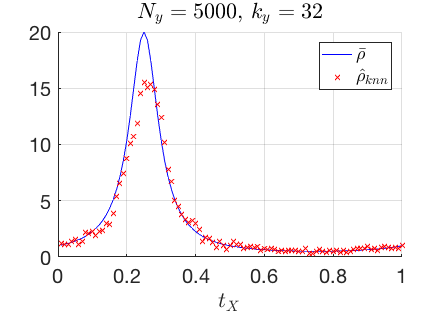
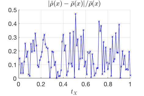
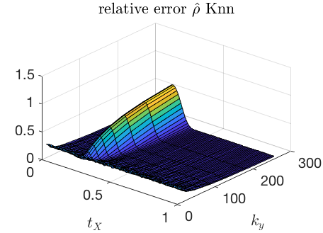
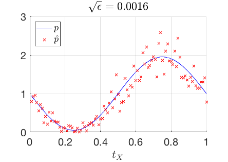
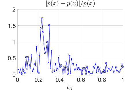
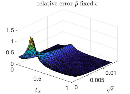
Figure 1: kNN estimation of $\bar{\rho}=p^{-1/d}$ and KDE estimation of $p$ for $x\in S^{1}$ embedded in $\mathbb{R}^{2}$, and $0\leq t_{X}\leq 1$ is the intrinsic coordinate (arclength). (Top) The left two plots show a typical realization of $\hat{\rho}$ by kNN defined in (6) compared with $\bar{\rho}$, and the right plot shows the relative error for varying values of $k_{y}$, $N_{y}=5000$, averaged over 500 runs. (Bottom) Same plots for $\hat{p}$ defined in (8) compared with $p$, and relative error for varying values of $\epsilon$.

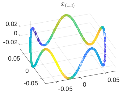
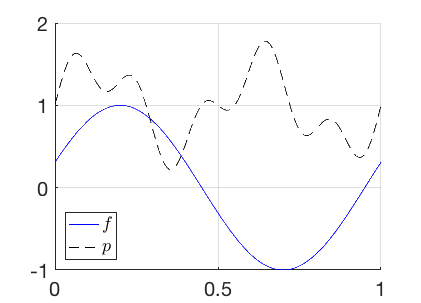
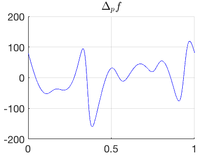
Figure 2: Data in $\mathbb{R}^{4}$ lying on a 1D closed curve of length 1. (Left) First 3 coordinates of 2000 samples with color indicating the density function $p$. (Middle) The density function $p$ and a function $f$, and (Right) $\Delta_{p}f$, all plotted v.s. the intrinsic coordinate (the arclength) on $[0,1]$.

4 Numerical Experiments

In this section, we denote the parameter $k$ as $k_{y}$ when the $k$NN estimation is conducted on the dataset $Y$. In Subsection 4.3, we use the notation $k_{x}$ when computing the $k$NN estimation on $X$.

4.1 kNN Estimator $\hat{\rho}$ of $\bar{\rho}=p^{-1/d}$

We numerically examine the kNN estimation of $\bar{\rho}$, namely $\hat{\rho}$ as defined in (6), and compare it with the fixed bandwidth KDE estimator $\hat{p}$ as in (8), where $h_{kde}(r):=e^{-r/(4/\pi)}$. The dataset is sampled from a circle of length 1 isometrically embedded in $\mathbb{R}^{2}$ i.i.d. according to a density function $p$, which equals 0.05 at ${\color[rgb]{0,0,0}t_{X}}=0.25$, $0\leq t_{X}\leq 1$ being the intrinsic coordinate (arclength), as shown in Fig. 1. The plots on the right hand side show the difference of the relative error at place where $p$ is low. As $k_{y}$ decreases ($\epsilon$ increases), the variance error starts to dominate, and $\hat{\rho}$ gives the relative error uniformly small across locations, as predicted by Theorem 2.3. In contrast, $\hat{p}$ gives a larger relative error near ${\color[rgb]{0,0,0}t_{X}}=0.25$. The result empirically verifies Theorem 2.3 and Remark 2.2.

4.2 Estimation of Dirichlet Form and $L_{N}f(x)$

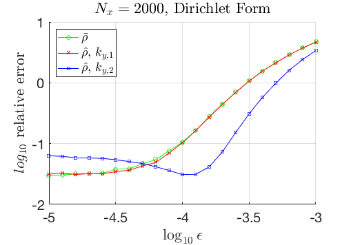
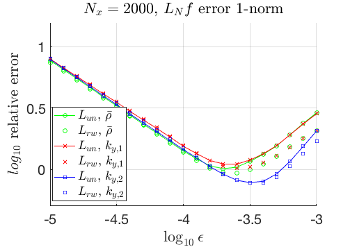
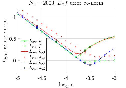
Figure 3: Relative error of (Left) Dirichlet form computed using $L_{un}$ and (Middle) $\text{Err}_{1}$ error in (20) of $L_{N}f$ computed by various $L_{N}$ plotted v.s. a range of values of $\epsilon$, $N_{y}=4000$, $k_{y}=32$, 256, averaged over 500 runs. (Right) Same plot for $\text{Err}_{\infty}$ error.

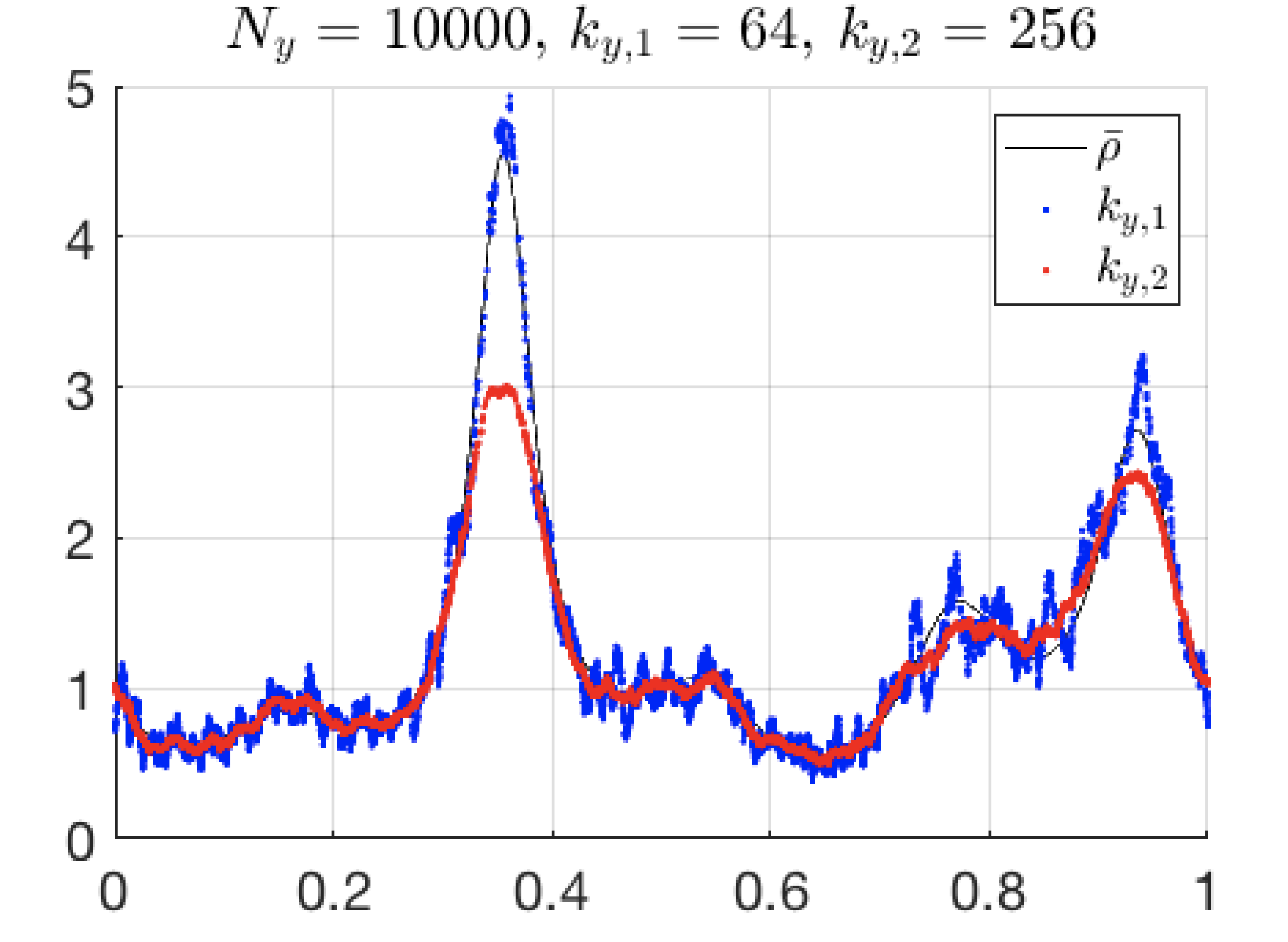
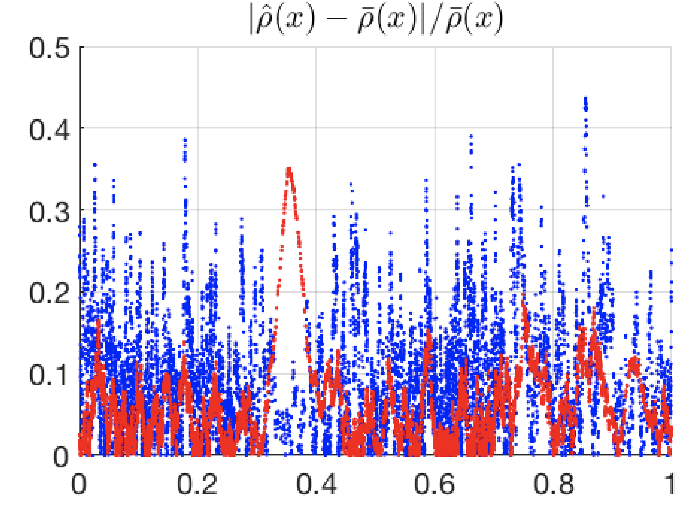
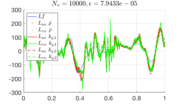
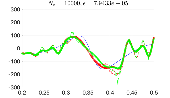
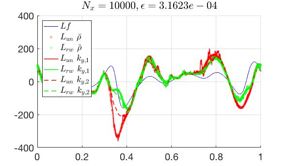
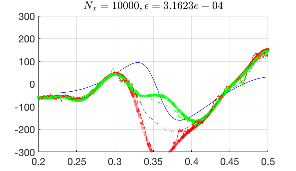
Figure 4: $L_{N}f$ by estimated $\hat{\rho}$ compared with true $\Delta_{p}f$, denoted as $Lf$ (blue curve), with two values of $k_{y}$. The data is as in Fig. 2. (Left) kNN-estimated $\hat{\rho}$ and relative errors. (Right upper) Estimated $L_{N}f$ where $L_{N}$ equals $L_{un}$ and $L_{rw^{\prime}}$, and using kNN-estimated $\hat{\rho}$, compared with using population $\bar{\rho}$. The right plot is the zoom in of the left plot on interval $[0.2,0.5]$. (Right bottom) Same plot as the right upper panel at another value of $\epsilon$. See more explanation in Section 4.2.

On the simulated data lying on a 1D smooth manifold embedded in $\mathbb{R}^{4}$ with a non-uniform density $p$ (Fig. 2), we compute self-tuned graph Laplacians on $N_{x}=2000$ data samples using (1) $L_{un}$ (17) and (2) $L_{rw^{\prime}}$ as in (18), $\alpha=1$, where $\hat{\rho}$ is estimated from a stand-alone dataset $Y$ with $N_{y}=4000$, and $k_{y}=32$, $256$ respectively. To evaluate the influence of $\bar{\rho}$ estimation, we also compute $L_{un}$ and $L_{rw^{\prime}}$ where $\hat{\rho}$ is replaced to be the true $\bar{\rho}$. The relative errors of

• The Dirichlet form $\langle f,\Delta_{p}f\rangle_{p}$,

• The point-wise error measure by

  $$\text{Err}_{1}:=\sum_{i=1}^{N_{x}}|L_{N}f(x_{i})-\Delta_{p}f(x_{i})|,\quad\text{Err}_{\infty}:=\max_{1\leq i\leq N_{x}}|L_{N}f(x_{i})-\Delta_{p}f(x_{i})|,$$ (20)

are given in Fig. 3. The error of $L_{N}f$ shows a scale of about $\epsilon^{-d/4-1/2}=\epsilon^{-0.75}$ in Fig. 3 right two plots, when the variance error dominates due to the small value of $\epsilon$. In comparison, the accuracy of Dirichlet form is less sensitive to the small value of $\epsilon$, as shown in Fig. 3(Left), which is consistent with the theoretical result in Theorems 3.3 and 3.5. Note that the relative 1-norm error shown in the plot divides $\text{Err}_{1}$ by $\|\{\Delta_{p}f(x_{i})\}_{i=1}^{N_{x}}\|_{1}$, thus its magnitude (about or greater than 1 in Fig. 3) depends on the choice of the test function $f$. Same with the relative $\infty$-norm error. When $N_{x}$ is increased to be 10,000, with the same $f$, the smallest relative error across $\epsilon$ is about 0.5 (averaged over 20 runs).

Taking $N_{x}=10,000$, $N_{y}=10,000$, with $k_{y}=64$, 256, respectively, we visualize in Fig. 4 snapshots of single realizations of $L_{N}f$. With smaller value of $\epsilon$, the estimated $L_{N}f$ has more oscillation around the true value, and when $\epsilon$ is larger, the oscillation is less but the function $L_{N}f$ is significantly biased at certain places on the manifold. Note that when $k_{y}$ is larger, the estimated $\hat{\rho}$ is smoother but has a significant bias at places where $p$ is small, and such bias is also reflected in the estimated $L_{N}f$. The two Laplacians, $L_{un}$ and $L_{rw^{\prime}}$, give comparable results.

4.3 The Influence of Stand-alone $Y$

We compare with the results using $X$ to estimate $\hat{\rho}$. The dataset is the same as that in Fig. 2. $N_{x}=2000$ and $k_{x}=32$ are used to compute $\hat{\rho}_{X}$. Take $N_{y}=\{2000,4000,\cdots,32000\}$ and $k_{y}=\{37,64,\cdots,338\}$, where $k_{y}$ is chosen to scale as $N_{y}^{4/5}$, according to Theorem 2.3 ($d=1$). The result for one realization with the largest $N_{y}$ is in Fig. 5, where using a stand-alone $Y$ of a much larger size than $X$ reduces the error in the estimated $\hat{\rho}$ as well as the oscillation in the estimated $L_{N}f$ (plots for $L_{rw^{\prime}}f$ are similar and not shown). The relative errors of Dirichlet form and $\text{Err}_{\infty}$ of $L_{N}f$ across $\epsilon$ are shown in Fig. 6, where using $\hat{\rho}_{X}$ and $\hat{\rho}_{Y}$ give comparable accuracy. Moreover, the result with $\hat{\rho}_{Y}$ approaches $L_{N}f$ computed from $\bar{\rho}$ as $N_{y}$ and $k_{y}$ increase. This suggests that when significantly more data samples than $N_{x}$ are available, using the rest as $Y$ to estimate the bandwidth function $\hat{\rho}$ may improve the estimation of the self-tuned graph Laplacian. With limited number of data samples, splitting stand-alone $Y$ may worsen the performance (due to decreasing $N_{x}$) than using the whole dataset as $X$ and estimating the bandwidth on itself.

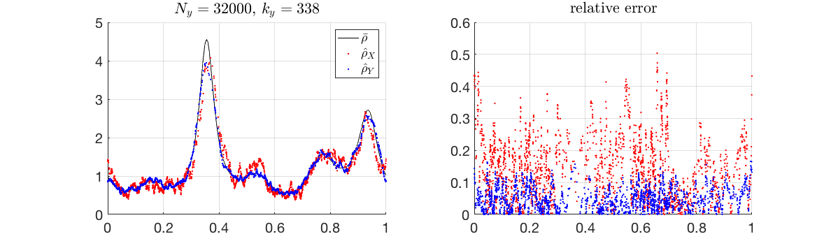
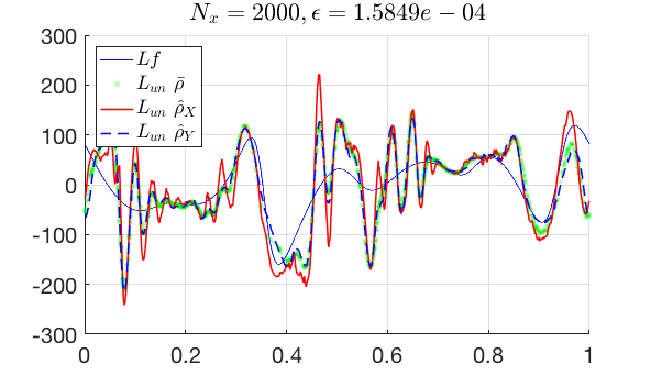
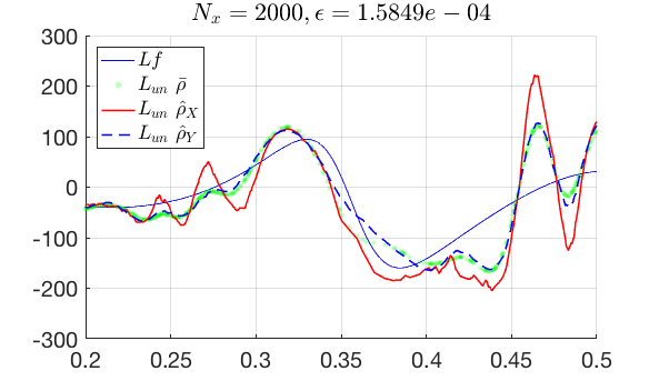
Figure 5: Same plots as Fig. 4 for self-tune Laplacian computed with $\hat{\rho}_{X}$. (Left two) kNN-estimated $\hat{\rho}$ and relative errors computed from $X$ and $Y$. (Right two) Estimated $L_{un}f$, with the zoom on the interval $[0.2,0.5]$.

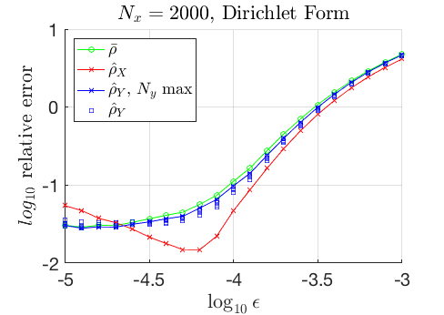
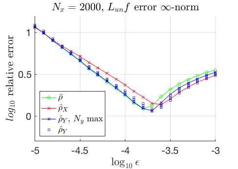
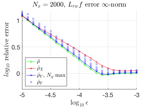
Figure 6: Relative error of (Left) Dirichlet form computed using $L_{un}$, and (Middle) $\text{Err}_{\infty}$ error of $L_{un}$ computed using $\bar{\rho}$, $\hat{\rho}_{X}$, and $\hat{\rho}_{Y}$ over a range of $\epsilon$ and different $\{N_{y},k_{y}\}$ (blue squares), averaged over 500 runs. (Right) Same plot for $L_{rw^{\prime}}$.

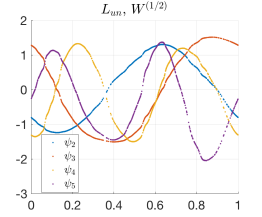
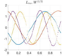
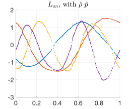
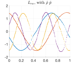
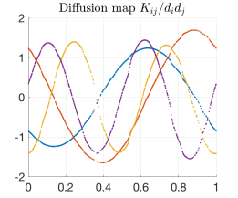
Figure 7: Plots of first 4 (non-trivial) eigenvectors of graph Laplacians which approximate eigenfunctions of $\Delta_{\mathcal{M}}$ of $S^{1}$. From left to right: $L_{un}$, $L_{rw^{\prime}}$ using $W^{(1-\frac{d}{2})}$; $L_{un}$, $L_{rw^{\prime}}$ using (21); degree $d_{i}^{-1}d_{j}^{-1}$normalized Diffusion Map [12]. Data as in Fig. 2, $N_{x}=1000$, the kNN self-tune bandwidth $\hat{\rho}$ computed from $X$ with $k_{x}=21$, $\epsilon=1e-4$.

4.4 Recovery of the Laplace-Beltrami Operator

According to the theory, the limiting operator is $\Delta_{\mathcal{M}}$ when $\alpha=1-\frac{d}{2}$. Here we examine two ways to recover $\Delta_{\mathcal{M}}$:

(1) By the self-tuned kernel affinity $W^{(1-\frac{d}{2})}$.

(2) By a normalization with a combination of $\hat{p}$ and $\hat{\rho}$,

$$W_{ij}=\frac{k_{0}\left(\frac{\|x_{i}-x_{j}\|^{2}}{\epsilon\hat{\rho}(x_{i})\hat{\rho}(x_{j})}\right)}{(\hat{\rho}\hat{p}^{1/2})(x_{i})(\hat{\rho}\hat{p}^{1/2})(x_{j})}=\frac{W^{(1)}_{ij}}{\hat{p}^{1/2}(x_{i})\hat{p}^{1/2}(x_{j})},$$ (21)

because $\bar{\rho}^{-d/2}=p^{1/2}$. The second approach does not need prior knowledge or estimation of the intrinsic dimensionality $d$, and thus can be applied in more general scenarios.

Consider the same 1D manifold data used in Fig. 2. Take $N_{x}=1000$, $\epsilon=10^{-4}$, and compute $\hat{\rho}$ from $X$. The embeddings by the first 4 (non-trivial) eigenvectors of various graph Laplacians are shown in Fig. 7, where the last column shows the result produced by affinity matrix $W_{ij}=\frac{K_{ij}}{d_{i}d_{j}}$, where $K_{ij}$ is the fix-bandwidth kernel affinity $K_{ij}=k_{0}(\frac{\|x_{i}-x_{j}\|^{2}}{\epsilon})$ and $d_{i}=\sum_{j}K_{ij}$, as in [12]. Recall that the eigenfunctions of the Laplace-Beltrami operator are sine and cosine functions with different frequencies. In this example, the random-walk graph Laplacian produces a visually better eigenfunction approximation compared with the unnormalized graph Laplacian. We postpone the study of the random-walk graph Laplacian with self-tuned kernel to future investigation.

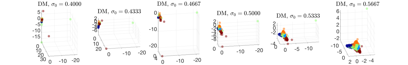
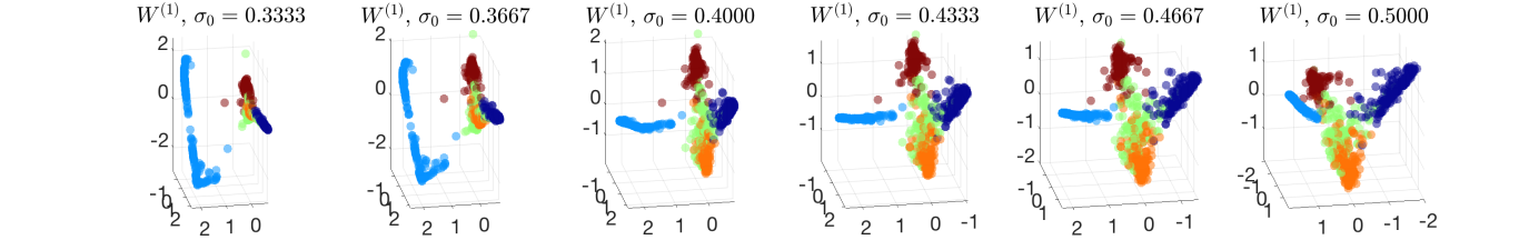
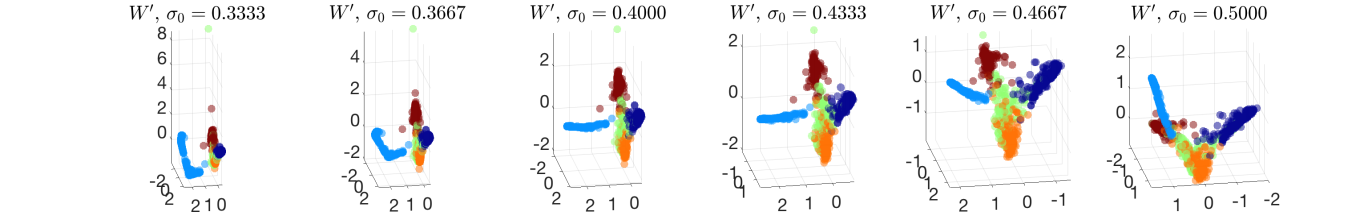
Figure 8: Eigenvector embedding of $N_{x}=$1000 MNIST hand-written digit images of 5 classes, $k_{x}=7$, colored by digit class labels. (Top) By $\frac{K_{ij}}{d_{i}d_{j}}$ with fixed-bandwidth kernel, (Middle) by self-tuned kernel $W^{(1)}$, (Bottom) by self-tuned kernel $W^{{}^{\prime}}$, as defined in (22).

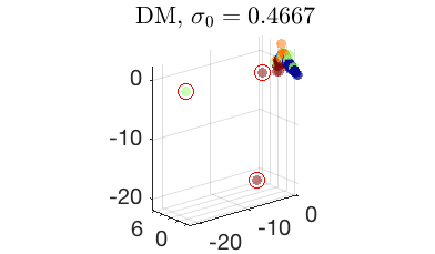
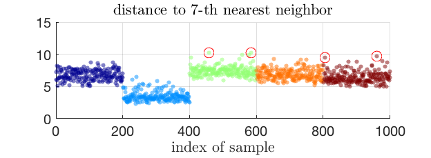
Figure 9: Outliers in the fixed-bandwidth kernel embedding. (Left) One embedding in the top panel of Fig. 8 with a proper rotation for visualization purpose, where the outlier samples are marked with red circles. (Right) Values of $\hat{R}_{i}$, i.e. the distance to the 7-th nearest neighbor, of the $N_{x}=$1000 samples. The outlier samples in the left plot are marked by red circles. The plot is colored by digit class labels.

4.5 Embedding of Hand-written Digits Data

We implement the embedding on $N_{x}=1000$ samples from the MNIST dataset, containing 5 classes (digits ‘0’, ‘1’, …, ‘4’) with 200 images in each class. The hand-written images can be viewed as lying near certain low-dimensional sub-manifolds in the $\mathbb{R}^{784}$ ambient space (each sample is a 28$\times$28 gray-scale image). We use $k_{x}=7$, and compute $\hat{R}_{i}$ as the $L^{2}$ distance between the $i$-th image to its $k_{x}$-th nearest neighbor. Also compute $\hat{\mu}_{i}:=\frac{1}{N}\sum_{j=1}^{N}h_{kde}(\frac{\|x_{i}-x_{j}\|^{2}}{\epsilon_{kde}})$, where $\epsilon_{kde}^{1/2}=\text{Median}_{i}\{\hat{R}_{i}\}$. Here, $\hat{\mu}$ is the (un-normalized) density estimator. Consider two self-tuned kernel affinities:

$$W_{ij}^{(1)}=k_{0}\left(\frac{\|x_{i}-x_{j}\|^{2}}{\sigma_{0}^{2}\hat{R}_{i}\hat{R}_{j}}\right)\frac{1}{\sigma_{0}^{2}\hat{R}_{i}\hat{R}_{j}},\quad W_{ij}^{{}^{\prime}}=k_{0}\left(\frac{\|x_{i}-x_{j}\|^{2}}{\sigma_{0}^{2}\hat{R}_{i}\hat{R}_{j}}\right)\frac{1}{\sigma_{0}^{2}\hat{R}_{i}\hat{R}_{j}\sqrt{\hat{\mu}_{i}\hat{\mu}_{j}}}\,.$$ (22)

We use $L_{rw^{\prime}}=D_{\hat{R}}^{-2}(D^{-1}W-I)$, where $W=W^{(1)}$ or $W^{{}^{\prime}}$, $(D_{\hat{R}})_{ii}=\sigma_{0}\hat{R}_{i}$, and $D$ is the degree matrix of $W$. The parameter $\sigma_{0}^{2}$ serves as the dimension-less bandwidth “$\epsilon$”. We also compare with the fixed-bandwidth kernel affinity matrix, where $\epsilon^{1/2}=\sigma_{0}\text{Median}_{i}(\hat{R}_{i})$, called the Diffusion Map (DM) embedding. The embeddings by the first 3 (non-trivial) eigenvectors over a range of values of $\sigma_{0}$ are shown in Fig. 8.

We observe that the DM embedding is disconnected at small value of $\sigma_{0}$ and consists of points which are far away from the bulk (outlier points), due to sensitivity to data points which are relatively farther away from its neighbor samples. As illustrated in Fig. 9, the outlier points in the DM embedding are those whose values of $\hat{R}_{i}$ are large. In comparison, both the self-tuned kernels provide informative embeddings of the dataset over the range of values of $\sigma_{0}$, showing improved stability at small values of $\sigma_{0}$ to data samples lying at places where the data density is low. The $W^{(1)}$ kernel affinity shows a better stability than the $W^{\prime}$ kernel at the small value of $\sigma_{0}$ on this dataset, due to that the $W^{\prime}$ kernel still involves a fixed-bandwidth KDE $\hat{\mu}$ in the normalization.

5 Proofs

5.1 Proofs in Section 2

Proof of Lemma 2.1.

Given $Y$ and $k>1$ fixed, define

$${\mathcal{S}}_{Y}:=\left\{x\in\mathbb{R}^{D},\,s.t.\,\exists j\neq j^{\prime},\,\|x-y_{j}\|=\|x-y_{j^{\prime}}\|\right\}\,.$$

Since $y_{j}$’s are distinct points, ${\mathcal{S}}_{Y}$ is a collection of finitely many hyperplanes in $\mathbb{R}^{D}$ (finitely many points when $D=1$), and ${\mathcal{S}}_{Y}\cap Y=\emptyset$. Whenever $x$ lies outside ${\mathcal{S}}_{Y}$, the set $\{\|x-y_{j}\|\}_{j=1}^{N}$ consists of distinct non-negative values. The set $\mathbb{R}^{D}\backslash{\mathcal{S}}_{Y}$ is open and consists of a finite union of polygons (the polygons can be unbounded), as illustrated in Fig. 10.

We prove the lemma in three parts as below.

Part 1: To prove that $\hat{R}$ is piece-wise $C^{\infty}$ on $\mathbb{R}^{D}\backslash{\mathcal{S}}_{Y}$, and on each polygon $\mathbf{p}$ in $\mathbb{R}^{D}\backslash{\mathcal{S}}_{Y}$, $\hat{R}(x)=\|x-y_{\mathbf{p}}\|$ for a point $y_{\mathbf{p}}\in Y$ and outside $\mathbf{p}$.

First, for each (open) polygon $\mathbf{p}$ and any $x\in\mathbf{p}$, the $k$-th nearest neighbor (kNN) of $x$ in $Y$ is uniquely defined due to the fact that the distance list $\{\|x-y_{j}\|\}_{j=1}^{N}$ has distinct values. Thus the function $\hat{R}(x)$ equals $\|x-y^{(k,x)}\|$, where $y^{(k,x)}$ is the kNN of $x$ in $Y$.

Second, we claim that the point $y^{(k,x)}$ is the same $y\in Y$ for all $x$ inside the polygon $\mathbf{p}$, because the ordered list of nearest neighbors is fixed for all $x$ within $\mathbf{p}$. Indeed, for the ordered list to cross, the distances of $\|x-y_{j}\|$ and $\|x-y_{j^{\prime}}\|$ need to be equal at some $x$, and this $x$ lies on ${\mathcal{S}}_{Y}$. We call this point $y_{\mathbf{p}}$, and then $\hat{R}(x)=\|x-y_{\mathbf{p}}\|$ for $x\in\mathbf{p}$.

Third, we claim that $y_{\mathbf{p}}\notin\mathbf{p}$. Note that each polygon $\mathbf{p}$ has at most one point $y_{j}$ inside it. Because otherwise, suppose $y_{j}\neq y_{j^{\prime}}$ are both inside $\mathbf{p}$, then so is the middle point $\frac{y_{j}+y_{j^{\prime}}}{2}$ due to that $\mathbf{p}$ is convex, but $\frac{y_{j}+y_{j^{\prime}}}{2}$ is in ${\mathcal{S}}_{Y}$ and cannot intersect with $\mathbf{p}$. Now if $y_{\mathbf{p}}\in\mathbf{p}$, then by definition $y_{\mathbf{p}}$ is the kNN of itself, which means that $k=1$. This contradicts with the condition that $k>1$.

The above gives us that $\hat{R}(x)=\|x-y_{\mathbf{p}}\|$ is $C^{\infty}$ and hence $\|\bar{\nabla}\hat{R}\|=1$ inside $\mathbf{p}$, by the fact that the mapping $x\mapsto\|x\|$ is $C^{\infty}$ on $\mathbb{R}^{D}\backslash\{0\}$. These properties hold for all polygons $\mathbf{p}$, thus $\hat{R}(x)$ is $C^{\infty}$ on $\mathbb{R}^{D}\backslash{\mathcal{S}}_{Y}$, and $\|\bar{\nabla}\hat{R}\|=1$ at point of differentiability.

Figure 10: Illustration of the set ${\mathcal{S}}_{Y}$ and example polygons in the proof of Lemma 2.1, $D=2$, $Y=\{y_{1},\cdots,y_{4}\}$, $k=2$, For each polygon $\mathbf{p}$, there is a point $y_{\mathbf{p}}\in Y$ such that $\hat{R}(x)=\|x-y_{\mathbf{p}}\|$ for $x\in\mathbf{p}$.

Part 2: To prove that $\text{Lip}_{\mathbb{R}^{D}}(\hat{R})\leq 1$.

We assume that $\hat{R}$ is continuous $\mathbb{R}^{D}$, which will be proved in Part 3. By Part 1, we have that $\hat{R}$ is Lipschitz 1 on each open polygon $\mathbf{p}$, and combined with the continuity of $\hat{R}$ at points on the boundary of $\mathbf{p}$, we have that $\text{Lip}_{\bar{\mathbf{p}}}(\hat{R})\leq 1$, where $\bar{\mathbf{p}}$ is the closure of $\mathbf{p}$, that is,

$$|\hat{R}(z)-\hat{R}(z^{\prime})|\leq\|z-z^{\prime}\|,\quad\forall z,z^{\prime}\in\bar{\mathbf{p}}.$$ (23)

For two points $x\neq x^{\prime}$ in $\mathbb{R}^{D}$, we want to show that $|\hat{R}(x)-\hat{R}(x^{\prime})|\leq\|x-x^{\prime}\|$. Consider the segment line $l$ connecting the two points. If $l$ is contained in some $\bar{\mathbf{p}}$, then the claim is proved. Otherwise, there is a sub-segment $l_{0}$ connecting from $x$ and $z_{1}\in{\mathcal{S}}_{Y}$ such that $l_{0}$ is in some $\bar{\mathbf{p}}$. Continue the process gives finitely many distinct points $\{z_{1},\cdots,z_{M}\}\subset l$ such that the sub-segment $l_{i}$ connecting from $z_{i}$ to $z_{i+1}$ is contained in some $\bar{\mathbf{p}}$ for $i=0$ to $M$, where $z_{0}=x$ and $z_{M+1}=x^{\prime}$. Note that this decomposition of $l$ into the union of $l_{i}$’s holds even when one or both of $x$ and $x^{\prime}$ are in ${\mathcal{S}}_{Y}$, as illustrated in Fig. 10.

Now by construction, $\|x-x^{\prime}\|=\sum_{i=0}^{M}\|z_{i}-z_{i+1}\|$. Meanwhile, applying (23) to each $l_{i}$ gives that $|\hat{R}(z_{i})-\hat{R}(z_{i+1})|\leq\|z_{i}-z_{i+1}\|$. Thus

$$|\hat{R}(x)-\hat{R}(x^{\prime})|\leq\sum_{i=0}^{M}|\hat{R}(z_{i})-\hat{R}(z_{i+1})|\leq\sum_{i=0}^{M}\|z_{i}-z_{i+1}\|=\|x-x^{\prime}\|.$$

Part 3: To prove that $\hat{R}$ is continuous on $\mathbb{R}^{D}$.

To finish the proof, it remains to prove the continuity of $\hat{R}$ on $\mathbb{R}^{D}$. For any $x_{0}\in\mathbb{R}^{D}$, let $\hat{R}(x_{0})=r_{0}$. Since $Y$ has distinct points by assumption, at most one point $y_{j}$ coincides with $x_{0}$. Since $k>1$, $r_{0}>0$. We prove that when $x\to x_{0}$, $\hat{R}(x)\to r_{0}$. Define

$$F(x,r):=\sum_{j=1}^{N}{\bf 1}_{\{\|x-y_{j}\|<r\}}\,.$$

Recall that

$$\hat{R}(x)=\inf\{r>0,\text{ s.t. }F(x,r)\geq k\}\,.$$

Since $F(x_{0},r)$ is monotonically increasing as $r$ increases, for any $r^{\prime}:=r_{0}+\varepsilon>r_{0}$, $F(x_{0},r^{\prime})\geq k$. This means that $|Y\cap B_{r^{\prime}}(x_{0})|:=k^{\prime}\geq k$. Since $B_{r^{\prime}}(x_{0})$ is an open ball, and there are $k^{\prime}$ many $y_{j}$’s lying inside it, they also all lie inside $B_{r^{\prime\prime}}(x_{0})$ where $r_{0}<r^{\prime\prime}<r^{\prime}$. Thus when $\|x-x_{0}\|<(r^{\prime}-r^{\prime\prime})/2:=r^{\prime\prime\prime}$, these $k^{\prime}$ points of $y_{j}$ also lie inside $B_{r^{\prime}}(x)$, then $F(x,r^{\prime})\geq k^{\prime}\geq k$. This gives that $\hat{R}(x)\leq r_{0}+\varepsilon$, whenever $\|x-x_{0}\|<r^{\prime\prime\prime}$.

Meanwhile, for any $0<r^{\prime}:=r_{0}-\varepsilon<r_{0}$, by definition $F(x_{0},r^{\prime}+\frac{\varepsilon}{2})<k$, i.e., $|Y\cap B_{r^{\prime}+\frac{\varepsilon}{2}}(x_{0})|:=k^{\prime}<k$. This means that for any $y\in Y\backslash B_{r^{\prime}+\frac{\varepsilon}{2}}(x_{0})$, the distance $\|y-x_{0}\|\geq r^{\prime}+\frac{\varepsilon}{2}$. Thus, when $\|x-x_{0}\|<\frac{\varepsilon}{4}$, the smallest distance $\|y-x\|$ for any $y\in Y\backslash B_{r^{\prime}+\frac{\varepsilon}{2}}(x_{0})$ is $\geq r^{\prime}+\frac{\varepsilon}{4}$, and then $F(x,r^{\prime})\leq k^{\prime}<k$. This shows that $\hat{R}(x)\geq r_{0}-\varepsilon$, whenever $\|x-x_{0}\|<\frac{\varepsilon}{4}$. Putting together, this proves the continuity of $\hat{R}(x)$ at $x_{0}$. ∎

Proof of Proposition 2.2.

Recall that $\bar{\rho}(x)=p(x)^{-1/d}$. Define

$$\bar{R}(x):=\bar{\rho}(x)\left(\frac{1}{m_{0}[h]}\frac{k}{N}\right)^{1/d}\,.$$ (24)

Then, since we have $\hat{\rho}(x)=\hat{R}(x)\left(\frac{1}{m_{0}[h]}\frac{k}{N}\right)^{-1/d}$ and $\bar{\rho}(x)=\bar{R}(x)\left(\frac{1}{m_{0}[h]}\frac{k}{N}\right)^{-1/d}$, the proposition can be equivalently proved by controlling $\frac{|\hat{R}(x)-\bar{R}(x)|}{\bar{R}(x)}$. For the given $s>0$, define

$$\delta_{r}:=t_{1}\left(\frac{k}{N}\right)^{2/d}+\frac{t_{2}}{d}\sqrt{\frac{s\log N}{k}}\,,$$ (25)

where $t_{1}=\Theta^{[p]}(1)$, $t_{2}=\Theta^{[1]}(1)$, both will be determined later. We will show that, when $N$ exceeds a threshold depending on $(p,s)$, for any $x\in{\mathcal{M}}$ fixed, w.p. greater than $1-2N^{-s/4}$,

$$\bar{R}(x)(1-\delta_{r})\leq\hat{R}(x)\leq\bar{R}(x)(1+\delta_{r}).$$ (26)

To prove (26), we introduce some notations. Denote

$$R_{-}(x):=\bar{R}(x)(1-\delta_{r}),\quad\mbox{and}\quad R_{+}(x)=\bar{R}{(x)}(1+\delta_{r})\,.$$

Let $h={\bf 1}_{[0,1)}$, and define, for any $x\in\mathcal{M}$ and $r>0$,

$$\hat{\mu}(x,r):=\frac{1}{N}\sum_{j=1}^{N}h\left(\frac{\|x-y_{j}\|^{2}}{r^{2}}\right)=:\frac{1}{N}\sum_{j=1}^{N}H_{j}(x,r)\,,$$

then, by (6), $\hat{R}(x)=\inf_{r}\left\{r>0,\,\text{ s.t. }\hat{\mu}(x,r)\geq\frac{k}{N}\right\}$. For fixed $x$ and $r$, $H_{j}$ are i.i.d. random variables, and

$$\mathbb{E}H_{j}(x,r)=\int_{\mathcal{M}}h\left(\frac{\|x-y\|^{2}}{r^{2}}\right)p(y)dV(y)=:\mu(x,r).$$ (27)

Below, to simplify notation, we omit the dependence on $x$ in $\bar{R}$, $R_{\pm}$ and $H_{j}$ when there is no confusion. The argument is for a fixed $x$, and we make sure that the constants $t_{1}$ and $t_{2}$ in $\delta_{r}$ as well as the large-$N$ threshold are uniform for all $x$.

Figure 11: Given a dataset $Y$ and a fixed $x$, plots of $\hat{\mu}(x,r)$, $\mu(x,r)$ and $m_{0}[h]p(x)r^{d}$ as functions of $r$. The values of $\hat{R}(x)$, $\bar{R}(x)$ and $R_{\pm}$ are marked. These quantities are used in the proof of Proposition 2.2.

We first address the lower bound in (26). By definition, $\hat{\mu}(x,r)$ is monotonically increasing on $(0,\infty)$. We claim that

$$\Pr[\hat{R}(x)<R_{-}]\leq\Pr\left[\hat{\mu}(x,R_{-})\geq\frac{k}{N}\right].$$ (28)

Because $\hat{R}(x)=\inf\{r>0,\hat{\mu}(x,r)\geq\frac{k}{N}\}$, if $\hat{R}(x)<R_{-}$, there is some $r^{\prime}$, $\hat{R}(x)<r^{\prime}<R_{-}$ such that $\hat{\mu}(x,r^{\prime})\geq\frac{k}{N}$, and by monotonicity $\hat{\mu}(x,R_{-})\geq\hat{\mu}(x,r^{\prime})\geq\frac{k}{N}$.

To bound the probability $\Pr\left[\hat{\mu}(x,R_{-})\geq\frac{k}{N}\right]$, we use that the expectation $\mu(x,R_{-})$ would be smaller than $\frac{k}{N}$ under some conditions for $\delta_{r}$ defined in (25).

Note that by definition (24), $\bar{R}(x)=\Theta^{[p]}((\frac{k}{N})^{1/d})=o^{[p]}(1)$, and the implied constant is uniform for all $x$ by the uniform boundedness of $\bar{\rho}$. Also, we have that $\delta_{r}=o^{[p]}(1)$ under the asymptotic condition on $k$. As a result, we have that

$$R_{-}=\Theta^{[p]}(\bar{R}(x))=\Theta^{[p]}\left((\frac{k}{N})^{1/d}\right)=o^{[p]}(1).$$ (29)

Then, Lemma A.4 gives that when $N$ is sufficiently large and then $R_{-}$ is small,

$$\mu(x,R_{-}) =m_{0}[h]p(x)R_{-}^{d}+O^{[p]}(R_{-}^{d+2})$$

$$=m_{0}[h]p(x)\bar{R}^{d}(1-\delta_{r})^{d}+O^{[p]}(\bar{R}^{d+2})$$

$$=m_{0}[h]p(x)\bar{R}^{d}\left(1-d\delta_{r}+O^{{\color[rgb]{0,0,0}[1]}}(\delta_{r}^{2})+O^{[p]}(\bar{R}^{2})\right)$$

$$\leq\frac{k}{N}(1-0.9d\delta_{r})+O^{[p]}(\bar{R}^{d+2})=:\frac{k}{N}-\delta_{\mu_{-}}\,,{\color[rgb]{0,0,0}~{}~{}~{}\text{(by that $m_{0}[h]p(x)\bar{R}^{d}=\frac{k}{N}$)}}$$ (30)

where the inequality in the last row is obtained by that $\delta_{r}=o^{[p]}(1)$, and the large-$N$ threshold here only depends on $p$. Note that the implied constant of $O^{[p]}(\bar{R}^{d+2})$, denoted as $c_{p}$, is uniform for all $x$. Meanwhile, by uniform boundedness of $p$ from below, we have

$$\bar{R}(x)\leq\max_{x\in{\mathcal{M}}}\bar{\rho}(x)\left(\frac{1}{m_{0}[h]}\frac{k}{N}\right)^{1/d}=\left(\frac{1}{{\color[rgb]{0,0,0}p_{min}}m_{0}[h]}\right)^{1/d}\left(\frac{k}{N}\right)^{1/d}\,.$$

Denote $c_{p,1}:=\left({\color[rgb]{0,0,0}p_{min}}m_{0}[h]\right)^{-1/d}$, and choose

$$t_{1}:=\frac{c_{p}c_{p,1}^{d+2}}{0.8d}{\color[rgb]{0,0,0}=\Theta^{[p]}(1)},$$ (31)

which is uniform for all $x$, then $t_{1}\cdot 0.9d\left(\frac{k}{N}\right)^{1+2/d}>c_{p}c_{p,1}^{d+2}\left(\frac{k}{N}\right)^{1+2/d}\geq c_{p}\bar{R}^{d+2}$. Thus, when $N$ is sufficiently large and the threshold depends on $p$, we have

$$\delta_{\mu_{-}} =0.9d\frac{k}{N}\left(t_{1}\left(\frac{k}{N}\right)^{2/d}+\frac{t_{2}}{d}\sqrt{\frac{s\log N}{k}}\right)+O^{[p]}(\bar{R}^{d+2})$$

$$>t_{2}\cdot 0.9\frac{k}{N}\sqrt{\frac{s\log N}{k}}=t_{2}\cdot 0.9\left(\frac{k}{N}\right)^{1/2}\sqrt{\frac{s\log N}{N}}=:\tilde{s}.$$ (32)

To use the concentration of $\hat{\mu}(R_{-})$ at $\mu(R_{-})$, we compute the boundedness and variance of $H_{j}(R_{-})$. Because $0\leq h\leq 1$, so is $H_{j}$, and then $|H_{j}|\leq L_{H}=1$. The variance

$$\text{Var}(H_{j})\leq\mathbb{E}H_{j}^{2}=\int_{\mathcal{M}}h^{2}\left(\frac{\|x-y\|^{2}}{R_{-}^{2}}\right)p(y)dV(y)=\mu(R_{-}),$$

because the kernel function $h:\mathbb{R}\to\mathbb{R}$ satisfies $h^{2}=h$. Thus, by that $\mu(R_{-})=m_{0}[h]p(x)R_{-}^{d}+O^{[p]}(R_{-}^{d+2})$ with (29), and that $\delta_{r}=o^{[p]}(1)$, when $N$ is sufficiently large,

$$\text{Var}(H_{j})\leq 1.1m_{0}[h]p(x)R_{-}^{d}\leq 1.5m_{0}[h]p(x)\bar{R}^{d}=1.5\frac{k}{N}=:\bar{\nu}_{H},$$

and the two inequalities hold when $N$ exceeds a threshold depending on $p$ only. By the classical Bernstein inequality, as long as $\tilde{s}L_{H}<3\bar{\nu}_{H}$, then

$$\Pr[\hat{\mu}(R_{-})-\mu(R_{-})>\tilde{s}]<e^{-\frac{1}{4}\tilde{s}^{2}\frac{N}{\bar{\nu}_{H}}}.$$

To verify that $\tilde{s}L_{H}<3\bar{\nu}_{H}$: note that it is equivalent to that $t_{2}\cdot 0.9<3\cdot 1.5(\frac{k}{s\log N})^{1/2}$, and since we have assumed $k=\Omega(\log N)$, if we have $t_{2}=\Theta(1)$, then it holds when $N$ is sufficiently large where the threshold depends on $s$. This is fulfilled by setting $t_{2}$ being an absolute constant such that

$$\frac{(t_{2}0.9)^{2}}{4\cdot 1.5}=1,{\color[rgb]{0,0,0}\quad 0<t_{2}<3}.$$ (33)

Thus, together with (30) and (32), we have

$$\mu(R_{-})\leq\frac{k}{N}-{\delta_{\mu_{-}}}<\frac{k}{N}-\tilde{s}\,.$$

As a result, (28) continues as

$$\Pr[\hat{R}(x)<R_{-}]\leq\Pr\left[\hat{\mu}(R_{-})\geq\frac{k}{N}\right]\leq\Pr\left[\hat{\mu}(R_{-})>\mu(R_{-})+\tilde{s}\right]<e^{-\frac{1}{4}\tilde{s}^{2}\frac{N}{\bar{\nu}_{H}}}=N^{-s},$$

which proves that w.p. higher than $1-N^{-s}$, the lower bound $\hat{R}(x)\geq R_{-}$ holds. We call the event $[\hat{R}(x)\geq R_{-}]$ the good event $E_{1}$. All the large-$N$ thresholds depend on $(p,s)$ and are uniform for all $x$.

The upper bound is proved in a similar way. Specifically,

$$\mu(R_{+}) =\frac{k}{N}(1+\delta r)^{d}+O^{[p]}(R_{+}^{d+2})\geq\frac{k}{N}(1+0.9d\delta r)+O^{[p]}(\bar{R}^{d+2})$$

$$=\frac{k}{N}+0.9d\frac{k}{N}\left(t_{1}(\frac{k}{N})^{2/d}+\frac{t_{2}}{d}\sqrt{\frac{s\log N}{k}}\right)+O^{[p]}(\bar{R}^{d+2}),$$

and the implied constant in $O^{[p]}(\bar{R}^{d+2})$, $c_{p}$, is same as the above by Lemma A.4. Then, again by the uniform upper bound of $\bar{R}(x)$ by $c_{p,1}(\frac{k}{N})^{1/d}$, by setting $t_{1}$ to be that in (31), we have

$$\mu(R_{+})>\frac{k}{N}+t_{2}0.9\left(\frac{k}{N}\right)^{1/2}\sqrt{\frac{s\log N}{N}}=\frac{k}{N}+\tilde{s}.$$

Same as before, $H_{j}(R_{+})$ is bounded by 1 and for a sufficiently large $N$,

$$\text{Var}(H_{j})\leq\mathbb{E}H_{j}^{2}=\mu(R_{+})\leq 1.5\frac{k}{N}=\bar{\nu}_{H}\,.$$

By letting $t_{2}$ as in (33), we have

$$\Pr[\hat{R}(x)>R_{+}]\leq\Pr\left[\hat{\mu}(R_{+})<\frac{k}{N}\right]\leq\Pr\left[\hat{\mu}(R_{+})<\mu(R_{+})-\tilde{s}\right]<e^{-\frac{1}{4}\tilde{s}^{2}\frac{N}{\bar{\nu}_{H}}}=N^{-s}.$$

This proves that w.p. higher than $1-N^{-s}$, the upper bound $\hat{R}(x)\leq R_{+}$ holds. We call the event $[\hat{R}(x)\leq R_{+}]$ the good event $E_{2}$.

Putting the above together, under the event $E_{1}\cap E_{2}$, which happens w.p. greater than $1-2N^{-s}$,

$$\frac{|\hat{R}(x)-\bar{R}(x)|}{\bar{R}(x)}\leq{\delta_{r}}=\frac{c_{p}c_{p,1}^{d+2}}{0.8d}\left(\frac{k}{N}\right)^{2/d}+\frac{\frac{2\sqrt{1.5}}{0.9}}{d}\sqrt{\frac{s\log N}{k}},$$

which proves the claim of the proposition. ∎

Proof of Theorem 2.3.

We restrict to when $Y$ has distinct points, which, under Assumption 2.1, holds w.p. 1, and then Lemma 2.1 holds.

We cover ${\mathcal{M}}$ using $r$-Euclidean balls, where $r>0$ is a constant of order $(k/N)^{3/d}$ with the implied constant to be determined. Suppose $N$ is large enough such that $r<\delta_{0}$ in Lemma A.1, then by Lemma A.2, we can find an $r$-net $F:=\{x_{1},\cdots,x_{n}\}$ whose cardinal number is $n$, $n{\leq}V({\mathcal{M}})r^{-d}$. We ask for the bound in Proposition 2.2 to hold at each $x_{i}$, where $s>0$ will be chosen later as an $\Theta^{[1]}(1)$ constant. Then, when $N$ exceeds a threshold depending on $p$ and uniform for all $x_{i}$, by a union bound, under a good event $E_{\hat{\rho},net}$ which happens w.p. higher than $1-2nN^{-s}$, we have

$$\left|\frac{\hat{\rho}(x_{i})}{\bar{\rho}(x_{i})}-1\right|\leq t_{1}\left(\frac{k}{N}\right)^{2/d}+\frac{t_{2}}{d}\sqrt{\frac{s\log N}{k}}:=\varepsilon,\quad\text{for all $i=1,\cdots,n$,}$$ (34)

where $t_{1}=\Theta^{[p]}(1)$ and $t_{2}=\Theta^{[1]}(1)$ are defined as in the proof of Proposition 2.2. Under the asymptotic condition on $k$, $\varepsilon=o^{[p]}(1)$ as $N\to\infty$.

We now consider $\hat{\rho}/\bar{\rho}$ on each $\bar{B}_{r}(x_{i})\cap{\mathcal{M}}$. Because $\bar{\rho}=p^{-1/d}$ is $C^{\infty}$ on ${\mathcal{M}}$, $\sup_{x\in{\mathcal{M}}}|\nabla_{\mathcal{M}}\bar{\rho}(x)|\leq L_{p}$. Then, for each $x_{i}$, by (A.2),

$$|\bar{\rho}(x)-\bar{\rho}(x_{i})|\leq L_{p}d_{\mathcal{M}}(x,x_{i})\leq 1.1L_{p}\|x-x_{i}\|\leq 1.1L_{p}r,\quad\forall x\in\bar{B}_{r}(x_{i})\cap{\mathcal{M}}.$$

Meanwhile, Lemma 2.1 gives that

$$\text{Lip}_{\mathbb{R}^{D}}(\hat{\rho})=\left(\frac{1}{m_{0}[h]}\frac{k}{N}\right)^{-1/d}\text{Lip}_{\mathbb{R}^{D}}(\hat{R})\leq\left(\frac{1}{m_{0}[h]}\frac{k}{N}\right)^{-1/d},$$

so we have

$$|\hat{\rho}(x)-\hat{\rho}(x_{i})|\leq\left(\frac{1}{m_{0}[h]}\frac{k}{N}\right)^{-1/d}r,\quad\text{$\forall x\in\bar{B}_{r}(x_{i})\cap{\mathcal{M}}$.}$$

Together, we have that $\forall x\in\bar{B}_{r}(x_{i})\cap{\mathcal{M}}$,

$$\left|\frac{\hat{\rho}(x)}{\bar{\rho}(x)}-\frac{\hat{\rho}(x_{i})}{\bar{\rho}(x_{i})}\right| \leq\frac{1}{\bar{\rho}(x)}\left|(\hat{\rho}(x))-\hat{\rho}(x_{i}))-\frac{\hat{\rho}(x_{i})}{\bar{\rho}(x_{i})}(\bar{\rho}(x)-\bar{\rho}(x_{i}))\right|$$

$$\leq{\frac{1}{{\rho}_{min}}}\left|\left(\frac{1}{m_{0}[h]}\frac{k}{N}\right)^{-1/d}+(1+\varepsilon)\cdot 1.1L_{p}\right|r=\Theta^{[p]}\left(\left({k}/{N}\right)^{-1/d}\right)r\,.$$ (35)

Thus, one can choose $r>0$ to be $\Theta^{[p]}((k/N)^{3/d})$ so as to make (35) bounded by $t_{1}(\frac{k}{N})^{2/d}$ when $N$ is sufficiently large, where the threshold of $N$ depends on $p$ only. This gives that $\left|\frac{\hat{\rho}(x)}{\bar{\rho}(x)}-\frac{\hat{\rho}(x_{i})}{\bar{\rho}(x_{i})}\right|\leq t_{1}(\frac{k}{N})^{2/d}$. Meanwhile, we already have (34) under $E_{\hat{\rho},net}$, and putting together,

$$\left|\frac{\hat{\rho}(x)}{\bar{\rho}(x)}-1\right|\leq\left|\frac{\hat{\rho}(x)}{\bar{\rho}(x)}-\frac{\hat{\rho}(x_{i})}{\bar{\rho}(x_{i})}\right|+\left|\frac{\hat{\rho}(x_{i})}{\bar{\rho}(x_{i})}-1\right|\leq t_{1}\left(\frac{k}{N}\right)^{2/d}+\varepsilon,\quad\forall x\in\bar{B}_{r}(x_{i})\cap{\mathcal{M}}.$$

By that $\mathcal{M}\subset\cup_{i}\bar{B}_{r}(x_{i})$, the above bound holds for all $x\in\mathcal{M}$. Recall the definition of $\varepsilon$ in (34), we have that, under $E_{\hat{\rho},net}$,

$$\sup_{x\in{\mathcal{M}}}\left|\frac{\hat{\rho}(x)}{\bar{\rho}(x)}-1\right|\leq 2t_{1}\left(\frac{k}{N}\right)^{2/d}+\frac{t_{2}}{d}\sqrt{\frac{s\log N}{k}}.$$

Finally, to show the high probability of $E_{\hat{\rho},net}$, by that $n\leq V({\mathcal{M}})r^{-d}$,

$$2nN^{-s} \leq 2V({\mathcal{M}})r^{-d}N^{-s}\leq c_{p}\left(\frac{k}{N}\right)^{-3}N^{-s}\quad\text{(constant $c_{p}$ depending on $p$)}$$

$$\leq N^{-s+3}.\quad\text{(with large $N$, because $k=\Omega(1)$)}$$

so by setting $s=13$, we have that $E_{\hat{\rho},net}$ happens w.p. higher than $>1-N^{-s+3}=1-N^{-10}$. ∎

5.2 Proof of Proposition 3.2

Proof of Proposition 3.2.

To simplify the notation, when there is no danger of confusion, we omit the dependence of $m_{l}[h]$ on $h$ and use the notation $m_{l}$, where $l=0,2$.

Under the condition that

$$\sup_{x\in{\mathcal{M}}}\frac{|\hat{\rho}(x)-\bar{\rho}(x)|}{|\bar{\rho}(x)|}<\varepsilon_{\rho}<0.1,$$ (36)

we have that

$$0.9\bar{\rho}(x)<\hat{\rho}(x)<1.1\bar{\rho}(x),\quad\forall x\in{\mathcal{M}}.$$ (37)

Recall that

$${\mathcal{E}}^{(\alpha)}(f,f)=\frac{\epsilon^{-\frac{d}{2}-1}}{m_{2}}\int_{\mathcal{M}}\int_{\mathcal{M}}(f(x)-f(y))^{2}k_{0}\left(\frac{\|x-y\|^{2}}{\epsilon\hat{\rho}(x)\hat{\rho}(y)}\right)\frac{p(x)p(y)}{\hat{\rho}(x)^{\alpha}\hat{\rho}(y)^{\alpha}}dV(x)dV(y)=:①,$$

and we consider the counterpart of $①$ where $\hat{\rho}(x)$ is replaced with $\bar{\rho}(x)$, namely,

$$②:=\frac{\epsilon^{-\frac{d}{2}-1}}{m_{2}}\int_{\mathcal{M}}\int_{\mathcal{M}}(f(x)-f(y))^{2}k_{0}\left(\frac{\|x-y\|^{2}}{\epsilon\bar{\rho}(x)\hat{\rho}(y)}\right)\frac{p(x)p(y)}{\bar{\rho}(x)^{\alpha}\hat{\rho}(y)^{\alpha}}dV(x)dV(y).$$

With the operator $G^{(\rho)}_{\epsilon}$ defined as in (14), writing the integration over $dV(x)$ via $G^{(\bar{\rho})}_{\epsilon}$,

$$② =\frac{1}{\epsilon m_{2}}\left(\int_{\mathcal{M}}(p\hat{\rho}^{d/2-\alpha})(y)G_{\epsilon\hat{\rho}(y)}^{(\bar{\rho})}\frac{f^{2}p}{\bar{\rho}^{\alpha}}(y)dV(y)-2\int_{\mathcal{M}}(fp\hat{\rho}^{d/2-\alpha})(y)G_{\epsilon\hat{\rho}(y)}^{(\bar{\rho})}\frac{fp}{\bar{\rho}^{\alpha}}(y)dV(y)\right.$$

$$~{}~{}~{}~{}~{}~{}~{}~{}~{}~{}\left.+\int_{\mathcal{M}}(f^{2}p\hat{\rho}^{d/2-\alpha})(y)G_{\epsilon\hat{\rho}(y)}^{(\bar{\rho})}\frac{p}{\bar{\rho}^{\alpha}}(y)dV(y)\right).$$ (38)

Recall that $\bar{\rho}=p^{-1/d}$ is in $C^{\infty}({\mathcal{M}})$ and uniformly bounded from below and above. By Lemma 3.1,

$$G_{\epsilon\hat{\rho}(y)}^{(\bar{\rho})}\frac{f^{2}p}{\bar{\rho}^{\alpha}} =m_{0}f^{2}p\bar{\rho}^{\frac{d}{2}-\alpha}+\epsilon\hat{\rho}\frac{m_{2}}{2}(\omega f^{2}p\bar{\rho}^{1+\frac{d}{2}-\alpha}+\Delta(f^{2}p\bar{\rho}^{1+\frac{d}{2}-\alpha}))+\hat{\rho}^{2}r_{1}^{(2)},$$

$$G_{\epsilon\hat{\rho}(y)}^{(\bar{\rho})}\frac{fp}{\bar{\rho}^{\alpha}} =m_{0}fp\bar{\rho}^{\frac{d}{2}-\alpha}+\epsilon\hat{\rho}\frac{m_{2}}{2}(\omega fp\bar{\rho}^{1+\frac{d}{2}-\alpha}+\Delta(fp\bar{\rho}^{1+\frac{d}{2}-\alpha}))+\hat{\rho}^{2}r_{2}^{(2)},$$

$$G_{\epsilon\hat{\rho}(y)}^{(\bar{\rho})}\frac{p}{\bar{\rho}^{\alpha}} =m_{0}p\bar{\rho}^{\frac{d}{2}-\alpha}+\epsilon\hat{\rho}\frac{m_{2}}{2}(\omega p\bar{\rho}^{1+\frac{d}{2}-\alpha}+\Delta(p\bar{\rho}^{1+\frac{d}{2}-\alpha}))+\hat{\rho}^{2}r_{3}^{(2)}\,,$$

where $\|r_{1}^{(2)}\|_{\infty}=O^{[f,p]}(\epsilon^{2})$, $\|r_{2}^{(2)}\|_{\infty}=O^{[f,p]}(\epsilon^{2})$ and $\|r_{3}^{(2)}\|_{\infty}=O^{[p]}(\epsilon^{2})$ and we omit the evaluation of all functions at $y$ in the notation. Then, (38) becomes

$$② =\frac{1}{\epsilon m_{2}}\left(\int_{\mathcal{M}}(p\hat{\rho}^{d/2-\alpha})\left\{m_{0}f^{2}p\bar{\rho}^{\frac{d}{2}-\alpha}+\epsilon\hat{\rho}\frac{m_{2}}{2}(\omega f^{2}p\bar{\rho}^{1+\frac{d}{2}-\alpha}+\Delta(f^{2}p\bar{\rho}^{1+\frac{d}{2}-\alpha}))+\hat{\rho}^{2}r_{1}^{(2)}\right\}\right.$$

$$~{}~{}~{}~{}~{}-2\int_{\mathcal{M}}(fp\hat{\rho}^{d/2-\alpha})\left\{m_{0}fp\bar{\rho}^{\frac{d}{2}-\alpha}+\epsilon\hat{\rho}\frac{m_{2}}{2}(\omega fp\bar{\rho}^{1+\frac{d}{2}-\alpha}+\Delta(fp\bar{\rho}^{1+\frac{d}{2}-\alpha}))+\hat{\rho}^{2}r_{2}^{(2)}\right\}$$

$$~{}~{}~{}~{}~{}\left.+\int_{\mathcal{M}}(f^{2}p\hat{\rho}^{d/2-\alpha})\left\{m_{0}p\bar{\rho}^{\frac{d}{2}-\alpha}+\epsilon\hat{\rho}\frac{m_{2}}{2}(\omega p\bar{\rho}^{1+\frac{d}{2}-\alpha}+\Delta(p\bar{\rho}^{1+\frac{d}{2}-\alpha}))+\hat{\rho}^{2}r_{3}^{(2)}\right\}\right)$$

$$=\frac{1}{2}\int_{\mathcal{M}}p\hat{\rho}^{\frac{d}{2}-\alpha+1}\left\{\Delta(f^{2}p\bar{\rho}^{1+\frac{d}{2}-\alpha})-2f\Delta(fp\bar{\rho}^{1+\frac{d}{2}-\alpha})+f^{2}\Delta(p\bar{\rho}^{1+\frac{d}{2}-\alpha})\right\}$$

$$~{}~{}~{}~{}~{}+\frac{1}{\epsilon m_{2}}\int_{\mathcal{M}}p\hat{\rho}^{\frac{d}{2}-\alpha+2}(r_{1}^{(2)}-2fr_{2}^{(2)}+f^{2}r_{3}^{(2)})$$

$$=:②_{1}+②_{2}\,,$$

where again, we omit the evaluation of all functions at $y$ and the integration over $dV(y)$ in the notation, and same in below.

We first consider $②_{1}$. Note that, by defining $g:=p\bar{\rho}^{1+d/2-\alpha}$, the bracket inside the integrand becomes

$$\left\{\cdots\right\}=\Delta(f^{2}g)-2f\Delta(fg)+f^{2}\Delta g=2g|\nabla f|^{2}=2p\bar{\rho}^{1+d/2-\alpha}|\nabla f|^{2}\,.$$

We define $②_{1}^{\prime}$ by substituting $\hat{\rho}$ with $\bar{\rho}$ in $②_{1}$, namely,

$$②_{1}^{\prime}:=\frac{1}{2}\int_{\mathcal{M}}p\bar{\rho}^{\frac{d}{2}-\alpha+1}\left\{\cdots\right\},\quad②_{1}-②_{1}^{\prime}=\frac{1}{2}\int_{\mathcal{M}}p(\hat{\rho}^{\frac{d}{2}-\alpha+1}-\bar{\rho}^{\frac{d}{2}-\alpha+1})\left\{\cdots\right\},$$

Inserting the expression of $\{\cdots\}$, by the definition of $\bar{\rho}=p^{-1/d}$ and $p_{\alpha}$, we have

$$②_{1}^{\prime}=\int_{\mathcal{M}}p^{2}\bar{\rho}^{2+d-2\alpha}|\nabla f|^{2}=\int_{\mathcal{M}}p_{\alpha}|\nabla f|^{2}={\mathcal{E}}_{p_{\alpha}}(f,f),$$

and also

$$②_{1}-②_{1}^{\prime}=\int_{\mathcal{M}}p^{2}\bar{\rho}^{1+d/2-\alpha}|\nabla f|^{2}(\hat{\rho}^{\frac{d}{2}-\alpha+1}-\bar{\rho}^{\frac{d}{2}-\alpha+1}).$$

Since $p$ and $\bar{\rho}$ are positive, we have

$$|②_{1}-②_{1}^{\prime}|\leq\int_{\mathcal{M}}p^{2}\bar{\rho}^{1+d/2-\alpha}|\nabla f|^{2}|\hat{\rho}^{\frac{d}{2}-\alpha+1}-\bar{\rho}^{\frac{d}{2}-\alpha+1}|.$$

Let $\gamma:=d/2-\alpha+1\in\mathbb{R}$. By the Mean Value Theorem and (37), for any $y$, there exists $\xi>0$ between $\hat{\rho}(y)$ and $\bar{\rho}(y)$, $\xi^{\gamma-1}\leq\max\{1.1^{\gamma-1},0.9^{\gamma-1}\}\bar{\rho}(y)^{\gamma-1}$ such that

$$|\hat{\rho}(y)^{\gamma}-\bar{\rho}(y)^{\gamma}|=\gamma\xi^{\gamma-1}|\hat{\rho}(y)-\bar{\rho}(y)|\leq\gamma\max\{1.1^{\gamma-1},0.9^{\gamma-1}\}\bar{\rho}(y)^{\gamma-1}|\hat{\rho}(y)-\bar{\rho}(y)|\leq c_{\gamma}\bar{\rho}(y)^{\gamma}\varepsilon_{\rho},$$ (39)

where the last inequality comes from (36) and $c_{\gamma}:=\gamma\max\{1.1^{\gamma-1},0.9^{\gamma-1}\}$ is a constant determined by $\alpha$ and $d$. Then

$$|②_{1}-②_{1}^{\prime}|\leq c_{\gamma}\varepsilon_{\rho}\int_{\mathcal{M}}p^{2}\bar{\rho}^{1+d/2-\alpha}|\nabla f|^{2}\bar{\rho}^{\gamma}=c_{\gamma}\varepsilon_{\rho}\cdot②_{1}^{\prime},$$

which gives that

$$②_{1}=②_{1}^{\prime}(1+O(c_{\gamma}\varepsilon_{\rho}))={\mathcal{E}}_{p_{\alpha}}(f,f)(1+O^{[\alpha]}(\varepsilon_{\rho}))\,,$$ (40)

Next we bound $②_{2}$. By definition,

$$|②_{2}|\leq\frac{1}{\epsilon m_{2}}\int_{\mathcal{M}}p\hat{\rho}^{\frac{d}{2}-\alpha+2}(|r_{1}^{(2)}|+2|f||r_{2}^{(2)}|+|f|^{2}|r_{3}^{(2)}|)\,.$$

Again, by (37), $\hat{\rho}(y)^{{d}/{2}-\alpha+2}\leq\max\{1.1^{{d}/{2}-\alpha+2},0.9^{{d}/{2}-\alpha+2}\}\bar{\rho}(y)^{{d}/{2}-\alpha+2}:=c_{\alpha}^{\prime}\bar{\rho}(y)^{{d}/{2}-\alpha+2}$. Then

$$|②_{2}|\leq O^{[f,p]}(\epsilon)\int_{\mathcal{M}}c_{\alpha}^{\prime}p\bar{\rho}^{\frac{d}{2}-\alpha+2}=O^{[f,p]}(\epsilon).$$

Together with (40), we have that

$$②={\mathcal{E}}_{p_{\alpha}}(f,f)(1+O^{[\alpha]}(\varepsilon_{\rho}))+O^{[f,p]}(\epsilon).$$ (41)

It remains to bound $|②-①|$ to prove the same bound for $①$. Define

$$③:=\frac{\epsilon^{-\frac{d}{2}-1}}{m_{2}}\int_{\mathcal{M}}\int_{\mathcal{M}}(f(x)-f(y))^{2}k_{0}\left(\frac{\|x-y\|^{2}}{\epsilon\bar{\rho}(x)\hat{\rho}(y)}\right)\frac{p(x)p(y)}{\hat{\rho}(x)^{\alpha}\hat{\rho}(y)^{\alpha}}dV(x)dV(y)\,.$$

Then,

$$③-②=\frac{\epsilon^{-\frac{d}{2}-1}}{m_{2}}\int_{\mathcal{M}}\int_{\mathcal{M}}(f(x)-f(y))^{2}\left(\frac{\bar{\rho}(x)^{\alpha}}{\hat{\rho}(x)^{\alpha}}-1\right)k_{0}\left(\frac{\|x-y\|^{2}}{\epsilon\bar{\rho}(x)\hat{\rho}(y)}\right)\frac{p(x)p(y)}{\bar{\rho}(x)^{\alpha}\hat{\rho}(y)^{\alpha}}dV(x)dV(y).$$ (42)

By (36) and (37), we have that

$$\sup_{x\in{\mathcal{M}}}\left|\frac{\bar{\rho}(x)^{\alpha}}{\hat{\rho}(x)^{\alpha}}-1\right|=O^{[\alpha]}(\varepsilon_{\rho}),\quad\sup_{x\in{\mathcal{M}}}\left|\frac{\bar{\rho}(x)}{\hat{\rho}(x)}-1\right|=O^{[1]}(\varepsilon_{\rho})\,.$$ (43)

Note that by definition, $②\geq 0$. Therefore, by that $k_{0}\geq 0$ and $p$, $\bar{\rho}$, $\hat{\rho}>0$,

$$|③-②| \leq O^{[\alpha]}(\varepsilon_{\rho})\cdot\frac{\epsilon^{-\frac{d}{2}-1}}{m_{2}}\int_{\mathcal{M}}\int_{\mathcal{M}}(f(x)-f(y))^{2}k_{0}\left(\frac{\|x-y\|^{2}}{\epsilon\bar{\rho}(x)\hat{\rho}(y)}\right)\frac{p(x)p(y)}{\bar{\rho}(x)^{\alpha}\hat{\rho}(y)^{\alpha}}dV(x)dV(y)$$

$$=O^{[\alpha]}(\varepsilon_{\rho})②.$$

Together with (41), this gives that

$$③=②(1+O^{[\alpha]}(\varepsilon_{\rho}))={\mathcal{E}}_{p_{\alpha}}(f,f)(1+O^{[\alpha]}(\varepsilon_{\rho}))+O^{[f,p]}(\epsilon).$$ (44)

Meanwhile,

$$③-①=\frac{\epsilon^{-\frac{d}{2}-1}}{m_{2}}\int_{\mathcal{M}}\int_{\mathcal{M}}(f(x)-f(y))^{2}\left(k_{0}\left(\frac{\|x-y\|^{2}}{\epsilon\bar{\rho}(x)\hat{\rho}(y)}\right)-k_{0}\left(\frac{\|x-y\|^{2}}{\epsilon\hat{\rho}(x)\hat{\rho}(y)}\right)\right)\frac{p(x)p(y)}{\hat{\rho}(x)^{\alpha}\hat{\rho}(y)^{\alpha}}dV(x)dV(y),$$

and

$$k_{0}\left(\frac{\|x-y\|^{2}}{\epsilon\bar{\rho}(x)\hat{\rho}(y)}\right)-k_{0}\left(\frac{\|x-y\|^{2}}{\epsilon\hat{\rho}(x)\hat{\rho}(y)}\right)=k_{0}^{\prime}(\xi)\frac{\|x-y\|^{2}}{\epsilon\bar{\rho}(x)\hat{\rho}(y)}\left(1-\frac{\bar{\rho}(x)}{\hat{\rho}(x)}\right),$$

where $\xi$ is between $\frac{\|x-y\|^{2}}{\epsilon\bar{\rho}(x)\hat{\rho}(y)}$ and $\frac{\|x-y\|^{2}}{\epsilon\hat{\rho}(x)\hat{\rho}(y)}$. By (37), $\xi\geq\frac{\|x-y\|^{2}}{\epsilon 1.1\bar{\rho}(x)\hat{\rho}(y)}$, and then,

$$|k_{0}^{\prime}(\xi)|\leq a_{1}e^{-a\xi}\leq a_{1}e^{-a\frac{\|x-y\|^{2}}{\epsilon 1.1\bar{\rho}(x)\hat{\rho}(y)}}.$$

By (43), we have that

$$|③-①| \leq\frac{\epsilon^{-\frac{d}{2}-1}}{m_{2}}\int_{\mathcal{M}}\int_{\mathcal{M}}(f(x)-f(y))^{2}|k_{0}^{\prime}(\xi)|\frac{\|x-y\|^{2}}{\epsilon\bar{\rho}(x)\hat{\rho}(y)}\left|1-\frac{\bar{\rho}(x)}{\hat{\rho}(x)}\right|\frac{p(x)p(y)}{\hat{\rho}(x)^{\alpha}\hat{\rho}(y)^{\alpha}}dV(x)dV(y)$$

$$\leq O(\varepsilon_{\rho})\frac{\epsilon^{-\frac{d}{2}-1}}{m_{2}}\int_{\mathcal{M}}\int_{\mathcal{M}}(f(x)-f(y))^{2}a_{1}e^{-\frac{a}{1.1}\frac{\|x-y\|^{2}}{\epsilon\bar{\rho}(x)\hat{\rho}(y)}}\frac{\|x-y\|^{2}}{\epsilon\bar{\rho}(x)\hat{\rho}(y)}\frac{p(x)p(y)}{\hat{\rho}(x)^{\alpha}\hat{\rho}(y)^{\alpha}}dV(x)dV(y)$$

$$=O(\varepsilon_{\rho})\frac{\epsilon^{-\frac{d}{2}-1}}{m_{2}}\int_{\mathcal{M}}\int_{\mathcal{M}}(f(x)-f(y))^{2}k_{1}\left(\frac{\|x-y\|^{2}}{\epsilon\bar{\rho}(x)\hat{\rho}(y)}\right)\frac{p(x)p(y)}{\hat{\rho}(x)^{\alpha}\hat{\rho}(y)^{\alpha}}dV(x)dV(y)$$

$$=O(\varepsilon_{\rho})\frac{m_{2}[k_{1}]}{m_{2}[k_{0}]}\cdot\text{$③^{\prime}$}\,,$$ (45)

where $③^{\prime}$ is defined by replacing $k_{0}$ to be $k_{1}$ in $③$, where

$$k_{1}(r):=a_{1}re^{-\frac{a}{1.1}r}\,\,\text{ and }\,\,r\geq 0.$$

Since $k_{1}$ satisfies Assumption 3.1, our analysis of $②$ and $③$ with $k_{1}$ so far applies. Thus, by (41) and (44), we have

$$\text{$③^{\prime}$}={\mathcal{E}}_{p_{\alpha}}(f,f)(1+O^{[\alpha]}(\varepsilon_{\rho}))+O^{[f,p]}(\epsilon),$$

and then

$$|③-①|=O(\varepsilon_{\rho})({\mathcal{E}}_{p_{\alpha}}(f,f)(1+O^{[\alpha]}(\varepsilon_{\rho}))+O^{[f,p]}(\epsilon))={\mathcal{E}}_{p_{\alpha}}(f,f)O^{[\alpha]}(\varepsilon_{\rho})+O^{[f,p]}(\epsilon\varepsilon_{\rho}).$$

Inserting (44) gives that

$$①=③+{\mathcal{E}}_{p_{\alpha}}(f,f)O^{[\alpha]}(\varepsilon_{\rho})+O^{[f,p]}(\epsilon\varepsilon_{\rho})={\mathcal{E}}_{p_{\alpha}}(f,f)(1+O^{[\alpha]}(\varepsilon_{\rho}))+O^{[f,p]}(\epsilon).$$

This finishes the proof since ${\mathcal{E}}^{(\alpha)}(f,f)=①$. ∎

5.3 Proofs in Section 3.3 (Theorems 3.3 and 3.4)

Proof of Theorem 3.3.

Suppose $f$ is not a constant function, because otherwise $E_{N}(f,f)={\mathcal{E}}_{p_{\alpha}}(f,f)=0$ and the theorem holds. By definition,

$$E_{N}(f,f)=\frac{1}{N^{2}}\sum_{i,j=1}^{N}\frac{\epsilon^{-\frac{d}{2}-1}}{m_{2}}(f(x_{i})-f(x_{j}))^{2}W_{ij}^{(\alpha)}=\frac{1}{N^{2}}\sum_{i\neq j,\,i,j=1}^{N}V_{ij},$$ (46)

where

$$V_{ij}:=\frac{1}{\epsilon m_{2}}(f(x_{i})-f(x_{j}))^{2}\hat{K}(x_{i},x_{j}).$$

As (46) is a V-statistic, we study $\mathbb{E}E_{N}(f,f)$ and its variation away from $\mathbb{E}E_{N}(f,f)$ respectively.

$\bullet$ Calculation of $\mathbb{E}E_{N}(f,f)$. By definition,

$$\mathbb{E}E_{N}(f,f)=\frac{N-1}{N}\mathbb{E}V_{1,2}\,\,\mbox{ and }\,\,\mathbb{E}V_{1,2}={\mathcal{E}}^{(\alpha)}(f,f).$$

Applying Proposition 3.2 gives

$$\mathbb{E}V_{1,2}={\mathcal{E}}_{p_{\alpha}}(f,f)(1+O^{[\alpha]}(\varepsilon_{\rho}))+O^{[f,p]}(\epsilon).$$ (47)

$\bullet$ Bound the deviation of $E_{N}(f,f)-\mathbb{E}E_{N}(f,f)$. We use the decoupling trick to bound the deviation of a V-statistic by that of an independent sum over $\frac{N}{2}$ terms. Specifically, define $\tilde{V}_{ij}=V_{ij}-\mathbb{E}V_{ij}$. For any $t>0$, the Markov inequality gives us

$$\Pr\left[\frac{1}{N(N-1)}\sum_{i\neq j,i,j=1}^{N}\tilde{V}_{ij}>t\right]\leq e^{-st}\mathbb{E}\exp\left\{s\frac{1}{N(N-1)}\sum_{i\neq j,i,j=1}^{N}\tilde{V}_{ij}\right\}$$ (48)

where $s>0$ will be determined later. By a direct expansion, and denote by ${\mathcal{S}}_{N}$ the permutation group, we have

$$e^{-st}\mathbb{E}\exp\left\{s\frac{1}{N(N-1)}\sum_{i\neq j,i,j=1}^{N}\tilde{V}_{ij}\right\}=e^{-st}\mathbb{E}\exp\left\{s\frac{1}{N!}\sum_{\sigma\in{\mathcal{S}}_{N}}\frac{1}{N(N-1)}\sum_{i\neq j,i,j=1}^{N}\tilde{V}_{\sigma(i),\sigma(j)}\right\}$$

$$= e^{-st}\mathbb{E}\exp\left\{s\frac{1}{N!}\sum_{\sigma\in{\mathcal{S}}_{N}}\frac{1}{N/2}\sum_{l=1}^{N/2}\tilde{V}_{\sigma(2l-1),\sigma(2l)}\right\}\leq e^{-st}\mathbb{E}\frac{1}{N!}\sum_{\sigma\in{\mathcal{S}}_{N}}\exp\left\{s\frac{1}{N/2}\sum_{l=1}^{N/2}\tilde{V}_{\sigma(2l-1),\sigma(2l)}\right\}$$

$$= e^{-st}\mathbb{E}\exp\left\{s\frac{1}{N/2}\sum_{l=1}^{N/2}\tilde{V}_{2l-1,2l}\right\},$$

where we apply the Jensen’s inequality in the inequality. Then, as in the derivation of the Classical Bernstein’s inequality, one can bound the probability in (48) by

$$\Pr[\cdots]\leq\exp\left\{-\frac{\frac{N}{2}t^{2}}{2\nu+\frac{2}{3}tL}\right\},\quad\text{where}\quad\nu:=\mathbb{E}\tilde{V}_{1,2}^{2},\quad|\tilde{V}_{1,2}|\leq L.$$ (49)

Below, we control $\nu$ and $L$. We first show that we can make $L=\Theta^{[f,p]}(\epsilon^{-\frac{d}{2}})$. Recall that

$$V_{1,2}=\frac{\epsilon^{-\frac{d}{2}-1}}{m_{2}}k_{0}\left(\frac{\|x_{1}-x_{2}\|^{2}}{\epsilon\hat{\rho}(x_{1})\hat{\rho}(x_{2})}\right)\frac{(f(x_{1})-f(x_{2}))^{2}}{\hat{\rho}(x_{1})^{\alpha}\hat{\rho}(x_{2})^{\alpha}}\,.$$

By Assumption A.3(C2’) for the kernel $k_{0}$,

$$|V_{1,2}|\leq\frac{\epsilon^{-\frac{d}{2}-1}}{m_{2}}a_{0}e^{-a\left(\frac{\|x_{1}-x_{2}\|^{2}}{\epsilon\hat{\rho}(x_{1})\hat{\rho}(x_{2})}\right)}\frac{(f(x_{1})-f(x_{2}))^{2}}{\hat{\rho}(x_{1})^{\alpha}\hat{\rho}(x_{2})^{\alpha}}.$$

By the assumption and (37), $\hat{\rho}(x)\leq 1.1\bar{\rho}(x)<1.1\rho_{max}$ for any $x$. Then when $\|x_{1}-x_{2}\|\geq\delta_{\epsilon}:=\sqrt{\epsilon 1.1^{2}\rho_{max}^{2}\frac{5+d/2}{a}\log\frac{1}{\epsilon}}$,

$$e^{-a\left(\frac{\|x_{1}-x_{2}\|^{2}}{\epsilon\hat{\rho}(x_{1})\hat{\rho}(x_{2})}\right)}\leq e^{-(5+d/2)\log\frac{1}{\epsilon}}=\epsilon^{5+d/2}$$

and then

$$|V_{1,2}|\leq\frac{a_{0}\epsilon^{4}}{m_{2}}\frac{(2\|f\|_{\infty})^{2}}{(0.9\rho_{min})^{2\alpha}}=O^{[f,p]}(\epsilon^{4}),\quad\text{ when $\|x_{1}-x_{2}\|\geq\delta_{\epsilon}$.}$$

Note that $\delta_{\epsilon}$ is of order $\sqrt{\epsilon\log(\epsilon^{-1})}$, since $\epsilon=o(1)$, when $\epsilon$ is small enough such that $\delta_{\epsilon}<\delta_{0}$ in Lemma A.1,

$$|f(x_{1})-f(x_{2})|\leq\|\nabla_{\mathcal{M}}f\|_{\infty}1.1\|x_{1}-x_{2}\|=:L_{f}\|x_{1}-x_{2}\|,\quad\text{for all $x_{2}\in B_{\delta_{\epsilon}}(x_{1})\cap{\mathcal{M}}$.}$$ (50)

Then, when $\|x_{1}-x_{2}\|<\delta_{\epsilon}$,

$$|V_{1,2}| \leq\frac{\epsilon^{-\frac{d}{2}-1}}{m_{2}}a_{0}e^{-a\left(\frac{\|x_{1}-x_{2}\|^{2}}{\epsilon\hat{\rho}(x_{1})\hat{\rho}(x_{2})}\right)}L_{f}^{2}\frac{\|x_{1}-x_{2}\|^{2}}{\hat{\rho}(x_{1})\hat{\rho}(x_{2})}\hat{\rho}(x_{1})^{1-\alpha}\hat{\rho}(x_{2})^{1-\alpha}$$

$$\leq\epsilon^{-\frac{d}{2}}\frac{a_{0}L_{f}^{2}}{m_{2}}a_{1}^{\prime}\|\max\{0.9^{1-\alpha},1.1^{1-\alpha}\}\bar{\rho}^{1-\alpha}\|_{\infty}^{2},$$

where $a_{1}^{\prime}$ equals an absolute constant times $\frac{a_{0}}{a}$. Combining both cases, $|V_{1,2}|=O^{[f,p]}(\epsilon^{-\frac{d}{2}})$, and we denote

$$|\tilde{V}_{1,2}|\leq L=\Theta^{[f,p]}(\epsilon^{-\frac{d}{2}}).$$

We now compute the variance $\nu$, and show that $\nu\leq\epsilon^{-d/2}V_{f}$ where $V_{f}=\Theta^{[f,p]}(1)$. By definition,

$$\mathbb{E}V_{1,2}^{2} =\int_{\mathcal{M}}\int_{\mathcal{M}}\frac{\epsilon^{-d-2}}{m_{2}[k_{0}]^{2}}k_{0}^{2}\left(\frac{\|x-y\|^{2}}{\epsilon\hat{\rho}(x)\hat{\rho}(y)}\right)\frac{(f(x)-f(y))^{4}}{\hat{\rho}(x)^{2\alpha}\hat{\rho}(y)^{2\alpha}}p(x)p(y)dV(x)dV(y)=\frac{\epsilon^{-d/2-1}}{\frac{m_{2}[k_{0}]^{2}}{m_{2}[k_{0}^{2}]}}\cdot④\,,$$ (51)

where

$$④ :=\frac{\epsilon^{-d/2-1}}{m_{2}[k_{0}^{2}]}\int_{\mathcal{M}}\int_{\mathcal{M}}k_{0}^{2}\left(\frac{\|x-y\|^{2}}{\epsilon\hat{\rho}(x)\hat{\rho}(y)}\right)\frac{(f(x)-f(y))^{4}}{\hat{\rho}(x)^{2\alpha}\hat{\rho}(y)^{2\alpha}}p(x)p(y)dV(x)dV(y).$$

Let $\delta_{\epsilon}$ be as above, and we separate the integral within and outside $\{\|x-y\|<\delta_{\epsilon}\}$ and make $④=④_{1}+④_{2}$. Specifically, we define

$$④_{2}:=\frac{\epsilon^{-d/2-1}}{m_{2}[k_{0}^{2}]}\int_{\mathcal{M}}\int_{\mathcal{M}}{\bf 1}_{\{\|x-y\|\geq\delta_{\epsilon}\}}k_{0}^{2}\left(\frac{\|x-y\|^{2}}{\epsilon\hat{\rho}(x)\hat{\rho}(y)}\right)\frac{(f(x)-f(y))^{4}}{\hat{\rho}(x)^{2\alpha}\hat{\rho}(y)^{2\alpha}}p(x)p(y)dV(x)dV(y)\,.$$

By a direct bound, we have

$$④_{2} \leq\frac{\epsilon^{-d/2-1}}{m_{2}[k_{0}^{2}]}\int_{\mathcal{M}}\int_{\mathcal{M}}a_{0}^{2}e^{-2a\left(\frac{\|x-y\|^{2}}{\epsilon\hat{\rho}(x)\hat{\rho}(y)}\right)}{\bf 1}_{\{\|x-y\|\geq\delta_{\epsilon}\}}(f(x)-f(y))^{4}\hat{\rho}(x)^{-2\alpha}\hat{\rho}(y)^{-2\alpha}p(x)p(y)dV(x)dV(y)$$

$$\leq\frac{\epsilon^{-d/2-1}}{m_{2}[k_{0}^{2}]}a_{0}^{2}\epsilon^{10+d}\int_{\mathcal{M}}\int_{\mathcal{M}}(f(x)-f(y))^{4}\max\{0.9^{-2\alpha},1.1^{-2\alpha}\}^{2}\bar{\rho}(x)^{-2\alpha}\bar{\rho}(y)^{-2\alpha}p(x)p(y)dV(x)dV(y)$$

$$=O^{[f,p]}(\epsilon^{\frac{d}{2}+9}).$$

Define

$$④_{1}:=\frac{\epsilon^{-d/2-1}}{m_{2}[k_{0}^{2}]}\int_{\mathcal{M}}\int_{\mathcal{M}}{\bf 1}_{\{\|x-y\|<\delta_{\epsilon}\}}k_{0}^{2}\left(\frac{\|x-y\|^{2}}{\epsilon\hat{\rho}(x)\hat{\rho}(y)}\right)\frac{(f(x)-f(y))^{4}}{\hat{\rho}(x)^{2\alpha}\hat{\rho}(y)^{2\alpha}}p(x)p(y)dV(x)dV(y)\,.$$

To control $④_{1}$, which involves an integration over the $\delta_{\epsilon}$ ball, note that for $y\in B_{\delta_{\epsilon}}(x)\cap{\mathcal{M}}$, by Lemma A.1,

$$f(y)=f(x)+\nabla f(x)\cdot(y-x)+O^{[f]}(\|x-y\|^{2}),$$

and thus,

$$(f(y)-f(x))^{4}=(\nabla f(x)\cdot(y-x))^{4}+O^{[f]}(\|x-y\|^{5})\leq(|\nabla f(x)|\|y-x\|)^{4}+O^{[f]}(\|x-y\|^{5})\,.$$

We then have

$$④_{1} \leq\frac{\epsilon^{-d/2-1}}{m_{2}[k_{0}^{2}]}\int_{\mathcal{M}}\int_{\mathcal{M}}{\bf 1}_{\{\|x-y\|<\delta_{\epsilon}\}}k_{0}^{2}\left(\frac{\|x-y\|^{2}}{\epsilon\hat{\rho}(x)\hat{\rho}(y)}\right)\frac{|\nabla f(x)|^{4}\|x-y\|^{4}+O^{[f]}(\|x-y\|^{5})}{\hat{\rho}(x)^{2\alpha}\hat{\rho}(y)^{2\alpha}}p(x)p(y)dV(x)dV(y)$$

$$=\frac{\epsilon^{-d/2-1}}{m_{2}[k_{0}^{2}]}\int_{\mathcal{M}}\int_{\mathcal{M}}{\bf 1}_{\{\|x-y\|<\delta_{\epsilon}\}}k_{0}^{2}\left(\frac{\|x-y\|^{2}}{\epsilon\hat{\rho}(x)\hat{\rho}(y)}\right)\frac{|\nabla f(x)|^{4}\|x-y\|^{4}}{\hat{\rho}(x)^{2\alpha}\hat{\rho}(y)^{2\alpha}}p(x)p(y)dV(x)dV(y)$$

$$~{}~{}~{}+\frac{\epsilon^{-d/2-1}}{m_{2}[k_{0}^{2}]}\int_{\mathcal{M}}\int_{\mathcal{M}}{\bf 1}_{\{\|x-y\|<\delta_{\epsilon}\}}k_{0}^{2}\left(\frac{\|x-y\|^{2}}{\epsilon\hat{\rho}(x)\hat{\rho}(y)}\right)\frac{O^{[f]}(\|x-y\|^{5})}{\hat{\rho}(x)^{2\alpha}\hat{\rho}(y)^{2\alpha}}p(x)p(y)dV(x)dV(y)=:⑤+⑥.$$

We establish a lemma, which can be proved similarly as in deriving the limit of $①$ above, namely, by replacing $\hat{\rho}(x)$ with $\bar{\rho}(x)$ first and then putting back. The proof is postponed to Appendix B.

Lemma 5.1.

Under (36) and (37), suppose $k_{0}$ satisfies Assumption 3.1, $f\in C^{\infty}({\mathcal{M}})$ and $\alpha\in\mathbb{R}$, then

$$\epsilon^{-\frac{d}{2}}\int_{\mathcal{M}}\int_{\mathcal{M}}f(x)^{2}k_{0}\left(\frac{\|x-y\|^{2}}{\epsilon\hat{\rho}(x)\hat{\rho}(y)}\right)\frac{p(x)p(y)}{\hat{\rho}(x)^{\alpha}\hat{\rho}(y)^{\alpha}}dV(x)dV(y)=m_{0}[k_{0}]\int p^{2}f^{2}\bar{\rho}^{d-2\alpha}+O^{[f,p]}(\epsilon,\varepsilon_{\rho}).$$

We bound $⑤$ and $⑥$ respectively, where $⑤$ will dominate. By a direct bound, we have

$$|⑥|\leq O^{[f]}(\epsilon^{\frac{3}{2}})\frac{\epsilon^{-d/2}}{m_{2}[k_{0}^{2}]}\int_{\mathcal{M}}\int_{\mathcal{M}}k_{0}^{2}\left(\frac{\|x-y\|^{2}}{\epsilon\hat{\rho}(x)\hat{\rho}(y)}\right)\left(\frac{\|x-y\|^{2}}{\epsilon\hat{\rho}(x)\hat{\rho}(y)}\right)^{\frac{5}{2}}\hat{\rho}(x)^{\frac{5}{2}-2\alpha}\hat{\rho}(y)^{\frac{5}{2}-2\alpha}p(x)p(y)dV(x)dV(y)\,.$$

Note that there is $b_{6}>0$, determined by $a_{0}$ and $a$, such that

$$k_{0}(r)^{2}r^{5/2}\leq a_{0}^{2}e^{-2ar}r^{5/2}\leq b_{6}e^{-ar},\quad\forall r>0.$$

Thus,

$$k_{0}^{2}\left(\frac{\|x-y\|^{2}}{\epsilon\hat{\rho}(x)\hat{\rho}(y)}\right)\left(\frac{\|x-y\|^{2}}{\epsilon\hat{\rho}(x)\hat{\rho}(y)}\right)^{\frac{5}{2}}\leq b_{6}e^{-a\frac{\|x-y\|^{2}}{\epsilon\hat{\rho}(x)\hat{\rho}(y)}},$$

and then

$$|⑥|\leq O^{[f]}(\epsilon^{\frac{3}{2}})\frac{\epsilon^{-d/2}}{m_{2}[k_{0}^{2}]}\int_{\mathcal{M}}\int_{\mathcal{M}}b_{6}e^{-a\frac{\|x-y\|^{2}}{\epsilon\hat{\rho}(x)\hat{\rho}(y)}}\frac{p(x)p(y)}{\hat{\rho}(x)^{2\alpha-\frac{5}{2}}\hat{\rho}(y)^{2\alpha-\frac{5}{2}}}dV(x)dV(y).$$

Since the kernel $k_{6}(r):=b_{6}e^{-ar}$ satisfies Assumption 3.1, applying Lemma 5.1 with $f$ replaced by 1 and $\alpha$ replaced by $2\alpha-\frac{5}{2}$ gives that

$$|⑥|=O^{[f]}(\epsilon^{\frac{3}{2}})\frac{1}{m_{2}[k_{0}^{2}]}\left(m_{0}[k_{6}]\int p^{2}\bar{\rho}^{d-2(2\alpha-\frac{5}{2})}{\color[rgb]{0,0,0}+O^{[p]}(\epsilon,\varepsilon_{\rho})}\right)=O^{[f,p]}(\epsilon^{\frac{3}{2}}).$$

Write $G(x)=|\nabla f(x)|^{2}$. Clearly, since $f\in C^{\infty}(\mathcal{M})$, $G$ is in $C^{\infty}({\mathcal{M}})$. Define

$$k_{5}(r):=k_{0}^{2}(r)r^{2}\,.$$

Then, $k_{5}$ satisfies Assumption 3.1 and $m_{0}[k_{5}]=dm_{2}[k_{0}^{2}]$. As a result,

$$⑤ \leq\frac{\epsilon^{-d/2-1}}{m_{2}[k_{0}^{2}]}\int_{\mathcal{M}}\int_{\mathcal{M}}G(x)^{2}k_{0}^{2}\left(\frac{\|x-y\|^{2}}{\epsilon\hat{\rho}(x)\hat{\rho}(y)}\right)\frac{\|x-y\|^{4}}{\hat{\rho}(x)^{2\alpha}\hat{\rho}(y)^{2\alpha}}p(x)p(y)dV(x)dV(y)$$

$$=\frac{\epsilon}{m_{2}[k_{0}^{2}]}\epsilon^{-d/2}\int_{\mathcal{M}}\int_{\mathcal{M}}G(x)^{2}k_{0}^{2}\left(\frac{\|x-y\|^{2}}{\epsilon\hat{\rho}(x)\hat{\rho}(y)}\right)\left(\frac{\|x-y\|^{2}}{\epsilon\hat{\rho}(x)\hat{\rho}(y)}\right)^{2}\frac{p(x)p(y)}{\hat{\rho}(x)^{2\alpha-2}\hat{\rho}(y)^{2\alpha-2}}dV(x)dV(y)$$

$$=\frac{\epsilon}{m_{2}[k_{0}^{2}]}\epsilon^{-d/2}\int_{\mathcal{M}}\int_{\mathcal{M}}G(x)^{2}k_{5}\left(\frac{\|x-y\|^{2}}{\epsilon\hat{\rho}(x)\hat{\rho}(y)}\right)\frac{p(x)p(y)}{\hat{\rho}(x)^{2\alpha-2}\hat{\rho}(y)^{2\alpha-2}}dV(x)dV(y)$$

$$=\frac{\epsilon}{m_{2}[k_{0}^{2}]}\cdot\left(m_{0}[k_{5}]\int p^{2}G^{2}\bar{\rho}^{d-2(2\alpha-2)}+O^{[f,p]}(\epsilon,\varepsilon_{\rho})\right)$$

$$=\epsilon d\int p^{2}|\nabla f|^{4}\bar{\rho}^{d-2(2\alpha-2)}+O^{[f,p]}(\epsilon^{2},\epsilon\varepsilon_{\rho})$$

$$=\epsilon d\int|\nabla f|^{4}p^{1+\frac{4(\alpha-1)}{d}}+O^{[f,p]}(\epsilon^{2},\epsilon\varepsilon_{\rho})\,,$$

where the third equality holds by applying Lemma 5.1 with $f$ replaced by $G$ and $\alpha$ replaced by $2\alpha-2$. Putting together, we have that

$$④ \leq⑤+⑥+④_{2}$$

$$\leq\epsilon d\int|\nabla f|^{4}p^{1+\frac{4(\alpha-1)}{d}}{+O^{[f,p]}(\epsilon^{2},\epsilon\varepsilon_{\rho})}+O^{[f,p]}(\epsilon^{\frac{3}{2}})+O^{[f,p]}(\epsilon^{\frac{d}{2}+9})$$

$$=\epsilon d\int|\nabla f|^{4}p^{1+\frac{4(\alpha-1)}{d}}+O^{[f,p]}(\epsilon^{\frac{3}{2}},\,\epsilon\varepsilon_{\rho})\,.$$

Plugging the above bounds back to (51), this gives that

$$\text{Var}(V_{1,2}) \leq\mathbb{E}V_{1,2}^{2}\leq\frac{\epsilon^{-d/2-1}}{\frac{m_{2}[k_{0}]^{2}}{m_{2}[k_{0}^{2}]}}\left(\epsilon d\int|\nabla f|^{4}p^{1+\frac{4(\alpha-1)}{d}}+O^{[f,p]}(\epsilon^{\frac{3}{2}}{,\,\epsilon\varepsilon_{\rho}})\right)$$

$$=\frac{m_{2}[k_{0}^{2}]}{m_{2}[k_{0}]^{2}}\epsilon^{-d/2}\left(d\int|\nabla f|^{4}p^{1+\frac{4(\alpha-1)}{d}}+O^{[f,p]}(\epsilon^{\frac{1}{2}}{,\,\varepsilon_{\rho}})\right).$$

Since $f$ is not constant valued, $\int|\nabla f|^{4}p^{1+\frac{4(\alpha-1)}{d}}>0$, and by that $\epsilon^{1/2},\,\varepsilon_{\rho}=o(1)$, we have that with sufficiently large $N$,

$$\nu=\text{Var}(V_{1,2})\leq\Theta^{[1]}(\epsilon^{-d/2})\int|\nabla f|^{4}p^{1+\frac{4(\alpha-1)}{d}}=\epsilon^{-d/2}V_{f},$$

where

$$V_{f}:=\Theta^{[1]}\left(\int|\nabla f|^{4}p^{1+\frac{4(\alpha-1)}{d}}\right).$$

Back to (49), by that $\nu\leq\epsilon^{-d/2}V_{f}$ and then

$$\exp\{-\frac{\frac{N}{2}t^{2}}{2\nu+\frac{2}{3}tL}\}\leq\exp\{-\frac{\frac{N}{2}t^{2}}{2\epsilon^{-d/2}V_{f}+\frac{2}{3}tL}\},$$ (52)

we now control the r.h.s. Let $s=\Theta(1)$ to be determined, and we set

$$t=\sqrt{\epsilon^{-d/2}V_{f}\frac{s\log N}{N}}\,.$$

Since $L=\Theta^{[f,p]}(\epsilon^{-d/2})$, and by the condition that $\epsilon^{d/2}N=\Omega(\log N)$, $\frac{\log N}{N\epsilon^{d/2}}=o(1)$, and hence $t=o^{[f,p]}(1)$. With large $N$,

$$\frac{tL}{\epsilon^{-d/2}V_{f}}=\Theta^{[f,p]}\left(\sqrt{\frac{\epsilon^{-d/2}}{V_{f}}\frac{s\log N}{N}}\right)=o^{[f,p]}(1)\,.$$

Therefore, when $N$ is sufficiently large, we have $\frac{tL}{\epsilon^{-d/2}V_{f}}<3$. Then (52) bounds the tail probability in (49) to be less than $\exp\{-\frac{Nt^{2}}{8\epsilon^{-d/2}V_{f}}\}=N^{-s/8}$. Let $s=80$, and use the same argument to bound $\Pr[\frac{1}{N(N-1)}\sum_{i\neq j}\tilde{V}_{ij}<-t]$. We have that w.p. greater than $1-2N^{-10}$

$$\left|\frac{1}{N(N-1)}\sum_{i\neq j,i,j=1}^{N}\tilde{V}_{ij}\right|\leq\sqrt{\epsilon^{-d/2}V_{f}\frac{80\log N}{N}}=O\left(\sqrt{\frac{\log N}{N\epsilon^{d/2}}\int|\nabla f|^{4}p^{1+\frac{4(\alpha-1)}{d}}}\right).$$ (53)

Call the event set that (53) holds the event $E_{Dir}$.

At last,

$$E_{N}(f,f)=\left(1-\frac{1}{N}\right)\cdot\frac{1}{N(N-1)}\sum_{i\neq j}V_{ij},$$

and with (47) we have shown that under good event $E_{Dir}$,

$$\frac{1}{N(N-1)}\sum_{i\neq j}V_{ij}={\mathcal{E}}_{p_{\alpha}}(f,f)(1+O^{[\alpha]}(\varepsilon_{\rho}))+O^{[f,p]}(\epsilon)+O\left(\sqrt{\frac{\log N}{N\epsilon^{d/2}}\int|\nabla f|^{4}p^{1+\frac{4(\alpha-1)}{d}}}\right),$$

which is $O^{[f,p]}(1)$, thus $E_{N}(f,f)$ differs from it by $O^{[f,p]}(\frac{1}{N})=o^{[f,p]}(\sqrt{\frac{1}{N}})$, which is dominated by the variance error. This finishes the proof of the theorem. ∎

Proof of Theorem 3.4.

The proof uses same techniques as that of Theorem 3.3, and is simplified due to fixed bandwidth kernel. We track the influence of $\beta$ and $\varepsilon_{p}$ which differs from the proof of Theorem 3.3. Inherit the notations in the proof of Theorem 3.3, the random variable $V_{ij}$ is now

$$V_{ij}:=\frac{\epsilon^{-\frac{d}{2}}}{\epsilon m_{2}}(f(x_{i})-f(x_{j}))^{2}k_{0}\left(\frac{\|x_{i}-x_{j}\|^{2}}{\epsilon}\right)\frac{1}{\hat{p}(x_{i})^{\beta}\hat{p}(x_{j})^{\beta}}.$$

Similarly as before, we define

$$①:=\mathbb{E}V_{ij}=\frac{1}{\epsilon m_{2}}\int\int(f(x)-f(y))^{2}\epsilon^{-\frac{d}{2}}k_{0}\left(\frac{\|x-y\|^{2}}{\epsilon}\right)\frac{p(x)p(y)}{\hat{p}(x)^{\beta}\hat{p}(y)^{\beta}}dV(x)dV(y),$$

and

$$② :=\frac{1}{\epsilon m_{2}}\int\int(f(x)-f(y))^{2}\epsilon^{-\frac{d}{2}}k_{0}\left(\frac{\|x-y\|^{2}}{\epsilon}\right)\frac{p(x)^{1-\beta}p(y)}{\hat{p}(y)^{\beta}}dV(x)dV(y),$$

$$③ :=\frac{1}{\epsilon m_{2}}\int\int(f(x)-f(y))^{2}\epsilon^{-\frac{d}{2}}k_{0}\left(\frac{\|x-y\|^{2}}{\epsilon}\right)p(x)^{1-\beta}p(y)^{1-\beta}dV(x)dV(y).$$

Define $q:=p^{1-\beta}$ which is a non-negative power of $p$ because $\beta\leq 1$, thus $q\in C^{\infty}(\mathcal{M})$. We then have

$$③ =\frac{1}{\epsilon m_{2}}\int\int(f(x)-f(y))^{2}\epsilon^{-\frac{d}{2}}k_{0}\left(\frac{\|x-y\|^{2}}{\epsilon}\right)q(x)q(y)dV(x)dV(y)$$

$$=\frac{2}{\epsilon m_{2}}\int\int(f(x)^{2}-f(x)f(y))\epsilon^{-\frac{d}{2}}k_{0}\left(\frac{\|x-y\|^{2}}{\epsilon}\right)q(x)q(y)dV(x)dV(y)$$

$$=\frac{2}{\epsilon m_{2}}\left(\int(qf^{2})G_{\epsilon}(q)-\int(qf)G_{\epsilon}(fq)\right).$$

By Lemma A.3,

$$G_{\epsilon}(q)=m_{0}q+\epsilon\frac{m_{2}}{2}(wq+\Delta q)+O^{[q^{(\leq 4)}]}(\epsilon^{2}),$$

$$G_{\epsilon}(fq)=m_{0}fq+\epsilon\frac{m_{2}}{2}(wfq+\Delta(fq))+O^{[(fq)^{(\leq 4)}]}(\epsilon^{2}),$$

and thus,

$$③ =\int qf(f\Delta q-\Delta(fq))+O^{[f,{\color[rgb]{0,0,0}q}]}(\epsilon)=-\int q^{2}f(\Delta f+2\frac{\nabla q}{q}\cdot\nabla f)+O^{[f,{\color[rgb]{0,0,0}q}]}(\epsilon)$$

$$=-\langle f,\Delta_{p_{\beta}}f\rangle_{p_{\beta}}+O^{[f,{\color[rgb]{0,0,0}q}]}(\epsilon)\quad\text{($p_{\beta}:=q^{2}=p^{2-2\beta}$)}$$

$$={\mathcal{E}}_{p_{\beta}}(f,f)+O^{[f,{\color[rgb]{0,0,0}q}]}(\epsilon).$$ (54)

To bound $|③-②|$: Because

$$③-②=\frac{1}{\epsilon m_{2}}\int\int(f(x)-f(y))^{2}\epsilon^{-\frac{d}{2}}k_{0}\left(\frac{\|x-y\|^{2}}{\epsilon}\right)p(x)^{1-\beta}p(y)(p(y)^{-\beta}-\hat{p}(y)^{-\beta})dV(x)dV(y),$$

by the positivity of $p$ and $k_{0}$,

$$|③-②|\leq\frac{1}{\epsilon m_{2}}\int\int(f(x)-f(y))^{2}\epsilon^{-\frac{d}{2}}k_{0}\left(\frac{\|x-y\|^{2}}{\epsilon}\right)p(x)^{1-\beta}p(y)|p(y)^{-\beta}-\hat{p}(y)^{-\beta}|dV(x)dV(y).$$

Note that for any $y$, by the Mean Value Theorem and that $|\hat{p}(y)-p(y)|/p(y)<\varepsilon_{p}<0.1$, $\exists\xi$ between $\hat{p}(y)$ and $p(y)$ and thus $\xi^{-\beta-1}\leq\max\{1.1^{-\beta-1},0.9^{-\beta-1}\}p(y)^{-\beta-1}$, and then we have

$$|\hat{p}(y)^{-\beta}-p(y)^{-\beta}| ={\color[rgb]{0,0,0}|\beta|}\xi^{-\beta-1}|\hat{p}(y)-p(y)|\leq{\color[rgb]{0,0,0}|\beta|}\max\{1.1^{-\beta-1},0.9^{-\beta-1}\}p(y)^{-\beta-1}|\hat{p}(y)-p(y)|$$

$$\leq c_{\beta}{\color[rgb]{0,0,0}|\beta|}p(y)^{-\beta}\varepsilon_{p},\quad c_{\beta}:=\max\{1.1^{-\beta-1},0.9^{-\beta-1}\}.$$ (55)

Thus,

$$|③-②|\leq{\color[rgb]{0,0,0}|\beta|}c_{\beta}\varepsilon_{p}\frac{1}{\epsilon m_{2}}\int\int(f(x)-f(y))^{2}\epsilon^{-\frac{d}{2}}k_{0}\left(\frac{\|x-y\|^{2}}{\epsilon}\right)p(x)^{1-\beta}p(y)^{1-\beta}dV(x)dV(y)={\color[rgb]{0,0,0}|\beta|}c_{\beta}\varepsilon_{p}③.$$

Combined with (54), we have that

$$② =③(1+O^{[1]}(\beta c_{\beta}\varepsilon_{p}))=({\mathcal{E}}_{p_{\beta}}(f,f)+O^{[f,{\color[rgb]{0,0,0}q}]}(\epsilon))(1+O^{[1]}(\beta c_{\beta}\varepsilon_{p}))$$

$$={\mathcal{E}}_{p_{\beta}}(f,f)(1+O^{[1]}({\color[rgb]{0,0,0}c_{\beta}}\beta\varepsilon_{p}))+O^{[f,{\color[rgb]{0,0,0}q}]}(\epsilon).$$ (56)

To bound $|②-①|$: By (55)

$$|②-①|\leq\frac{1}{\epsilon m_{2}}\int\int(f(x)-f(y))^{2}\epsilon^{-\frac{d}{2}}k_{0}\left(\frac{\|x-y\|^{2}}{\epsilon}\right)p(y)\hat{p}(y)^{-\beta}p(x)|p(x)^{-\beta}-\hat{p}(x)^{-\beta}|dV(x)dV(y)$$

$$\leq{\color[rgb]{0,0,0}|\beta|}c_{\beta}\varepsilon_{p}\frac{1}{\epsilon m_{2}}\int\int(f(x)-f(y))^{2}\epsilon^{-\frac{d}{2}}k_{0}\left(\frac{\|x-y\|^{2}}{\epsilon}\right)p(y)\hat{p}(y)^{-\beta}p(x)^{1-\beta}dV(x)dV(y)={\color[rgb]{0,0,0}|\beta|}c_{\beta}\varepsilon_{p}②.$$

Then, together with (56), we have that

$$\mathbb{E}V_{ij} =①=②(1+O^{[1]}(\beta c_{\beta}\varepsilon_{p}))=({\mathcal{E}}_{p_{\beta}}(f,f)(1+O^{[1]}(\beta{\color[rgb]{0,0,0}c_{\beta}}\varepsilon_{p}))+O^{[f,{\color[rgb]{0,0,0}q}]}(\epsilon))(1+O^{[1]}(\beta{\color[rgb]{0,0,0}c_{\beta}}\varepsilon_{p}))$$

$$={\mathcal{E}}_{p_{\beta}}(f,f)(1+O^{[1]}(\beta{\color[rgb]{0,0,0}c_{\beta}}\varepsilon_{p}))+O^{[f,{\color[rgb]{0,0,0}q}]}(\epsilon),{\color[rgb]{0,0,0}\quad\text{and }O^{[f,{\color[rgb]{0,0,0}q}]}(\epsilon)=O^{[f,{\color[rgb]{0,0,0}p,\beta}]}(\epsilon)\text{ by definition.}}$$

In the special case where $\beta=0$, we have $q=p$, and $①=②=③$. Then (54) gives that

$$\mathbb{E}V_{ij}=①={\mathcal{E}}_{p^{2}}(f,f)+O^{[f,p]}(\epsilon).$$

The boundedness of $|V_{ij}|$ follows by the same argument of truncation on the $\delta_{\epsilon}$ ball as in the proof of Theorem 3.3, which gives

$$|V_{ij}|\leq L=\Theta^{[f,p{\color[rgb]{0,0,0},\beta}]}(\epsilon^{-d/2}).$$

The variance

$$\text{Var}(V_{ij}) \leq\mathbb{E}V_{ij}^{2}=\int\int\frac{\epsilon^{-d-2}}{m_{2}^{2}}(f(x)-f(y))^{4}k_{0}^{2}\left(\frac{\|x_{i}-x_{j}\|^{2}}{\epsilon}\right)\frac{p(x)p(y)}{\hat{p}(x)^{2\beta}\hat{p}(y)^{2\beta}}dV(x)dV(y),$$

and, similarly as in the proof of Theorem 3.3, we can show that

$$\mathbb{E}V_{ij}^{2}\leq\epsilon^{-d/2}V_{f},\quad V_{f}=\Theta^{[1]}(\int|\nabla f|^{4}p^{2-4\beta}).$$

Thus, by the V-statistics decoupling argument, w.p. higher than $1-2N^{-10}$, the variance error is

$$O^{[1]}\left(\sqrt{\frac{\log N}{N\epsilon^{d/2}}\int|\nabla f|^{4}p^{2-4\beta}}\right).$$

The normalization $\frac{1}{N^{2}}$ and $\frac{1}{N(N-1)}$ in the V-statistics incurs higher order error, and putting together bias and variance error proves the theorem. ∎

5.4 Proofs in Section 3.4 (Theorems 3.5, 3.6, 3.7 and 3.8)

Proof of Theorem 3.5.

Define $\tilde{m}:=\frac{m_{2}}{2m_{0}}$, and rewrite (18) as

$$L^{(\alpha)}_{rw^{\prime}}f(x)=\frac{1}{\epsilon\tilde{m}\hat{\rho}(x)^{2}}\left(\frac{\frac{1}{N}\sum_{j=1}^{N}F_{j}(x)}{\frac{1}{N}\sum_{j=1}^{N}G_{j}(x)}-f(x)\right),$$ (57)

where

$$F_{j}:=\epsilon^{-d/2}k_{0}\left(\frac{\|x-x_{j}\|^{2}}{\epsilon\hat{\rho}(x)\hat{\rho}(x_{j})}\right)\frac{f(x_{j})}{\hat{\rho}(x_{j})^{\alpha}},\quad G_{j}:=\epsilon^{-d/2}{k_{0}\left(\frac{\|x-x_{j}\|^{2}}{\epsilon\hat{\rho}(x)\hat{\rho}(x_{j})}\right)}\frac{1}{\hat{\rho}(x_{j})^{\alpha}}.$$ (58)

Note that since $x_{j}$ $\sim p$ i.i.d., $\{F_{j}\}_{j=1}^{N}$ are i.i.d. rv’s, so are $\{G_{j}\}_{j=1}^{N}$, while $F_{j}$’s and $G_{j}$’s are dependent. The expectations are

$$\mathbb{E}F(x) =\epsilon^{-d/2}\int_{\mathcal{M}}{k_{0}\left(\frac{\|x-y\|^{2}}{\epsilon\hat{\rho}(x)\hat{\rho}(y)}\right)}\frac{f(y)}{\hat{\rho}(y)^{\alpha}}p(y)dV(y),$$

$$\mathbb{E}G(x) =\epsilon^{-d/2}\int_{\mathcal{M}}{k_{0}\left(\frac{\|x-y\|^{2}}{\epsilon\hat{\rho}(x)\hat{\rho}(y)}\right)}\frac{1}{\hat{\rho}(y)^{\alpha}}p(y)dV(y).$$

Following the strategy in [43, 6] to analyze the bias and variance errors respectively, we will show that

• The bias:

  $$\frac{1}{\epsilon\tilde{m}\hat{\rho}(x)^{2}}\left(\frac{\mathbb{E}F(x)}{\mathbb{E}G(x)}-f(x)\right)\overset{?}{=}{\mathcal{L}}^{(\alpha)}f(x)+O^{[f,p]}\left(\epsilon,\,\frac{\varepsilon_{\rho}}{\epsilon}\right)$$ (59)

• The variance:

  $$\frac{1}{\epsilon\tilde{m}\hat{\rho}(x)^{2}}\left(\frac{\frac{1}{N}\sum_{j=1}^{N}F_{j}(x)}{\frac{1}{N}\sum_{j=1}^{N}G_{j}(x)}-\frac{\mathbb{E}F(x)}{\mathbb{E}G(x)}\right)\overset{?}{=}O^{[1]}\left({\color[rgb]{0,0,0}\|\nabla f\|_{\infty}}p(x)^{1/d}\sqrt{\frac{\log N}{N\epsilon^{d/2+1}}}\right)$$ (60)

Proof of (59): By the definition of $G^{({\rho})}_{\epsilon}$ in (14),

$$\mathbb{E}F(x)=\hat{\rho}(x)^{d/2}G^{(\hat{\rho})}_{\epsilon\hat{\rho}(x)}(\frac{fp}{\hat{\rho}^{\alpha}})(x),$$

yet $\frac{fp}{\hat{\rho}^{\alpha}}$ is not $C^{4}$. In order to apply Lemma 3.1 and 3.2, we compare to replacing it with $\frac{fp}{\bar{\rho}^{\alpha}}$:

Lemma 5.2.

Suppose notation and condition are the same as those in Lemma 3.1 and 3.2. When $\epsilon$ is sufficiently small, for some constant $c_{\rho}^{\prime\prime}$ determined by $({\mathcal{M}},k_{0},\rho_{max},\rho_{min})$,

$$\sup_{x\in{\mathcal{M}}}|G_{\epsilon}^{(\tilde{\rho})}(\frac{f}{\tilde{\rho}^{\alpha}})(x)-G_{\epsilon}^{(\tilde{\rho})}(\frac{f}{{\rho}^{\alpha}})(x)|\leq c_{\rho}^{\prime\prime}\|f\|_{\infty}\varepsilon=O^{[f,\rho]}(\varepsilon).$$

The proof of Lemma 5.2 is postponed to Appendix B. Applying Lemmas 3.1, 3.2 and 5.2, where $\rho=\bar{\rho}$, $\tilde{\rho}=\hat{\rho}$ and “$f$” in the lemmas is replaced with $fp$, we have

$$\mathbb{E}F(x)=\hat{\rho}(x)^{d/2}\left(G^{(\hat{\rho})}_{\epsilon\hat{\rho}(x)}(\frac{fp}{\bar{\rho}^{\alpha}})(x)+O^{[f,p]}(\varepsilon_{\rho})\right)\quad\text{(by Lemma \ref{lemma:replace-hatrhoalpha-GR-hatrho})}$$

$$=\hat{\rho}(x)^{d/2}\left(G^{(\bar{\rho})}_{\epsilon\hat{\rho}(x)}(\frac{fp}{\bar{\rho}^{\alpha}})(x)+O^{[f,p]}(\varepsilon_{\rho})+O^{[f,p]}(\varepsilon_{\rho})\right)\quad\text{(by Lemma \ref{lemma:right-operator-repalce-rho})}$$

$$=\hat{\rho}(x)^{d/2}\left(m_{0}fp\bar{\rho}^{\frac{d}{2}-\alpha}(x)+\epsilon\hat{\rho}\frac{m_{2}}{2}(\omega fp\bar{\rho}^{1+\frac{d}{2}-\alpha}+\Delta(fp\bar{\rho}^{1+\frac{d}{2}-\alpha}))(x)+\hat{\rho}^{2}(x)O^{[f,p]}(\epsilon^{2})+O^{[f,p]}(\varepsilon_{\rho})\right),$$

where the residual terms in big-$O$ are bounded uniformly for all $x\in{\mathcal{M}}$. Below, we omit the variable $x$ in the notation when there is no confusion.

Because $0.9\bar{\rho}\leq\hat{\rho}\leq 1.1\bar{\rho}$ for all $x\in{\mathcal{M}}$, for any power $\gamma\in\mathbb{R}$, $\hat{\rho}^{\gamma}$ lies between $\bar{\rho}^{\gamma}1.1^{\gamma}$ and $\bar{\rho}^{\gamma}0.9^{\gamma}$ (the order depending on the sign of $\gamma$), and then uniformly bounded between $(0.9\rho_{min})^{\gamma}$ and $(1.1\rho_{max})^{\gamma}$, both of which are $\Theta^{[p]}(1)$ constants. We can also bound $|\hat{\rho}^{\gamma}-\bar{\rho}^{\gamma}|$ as in (39), and in summary we have

$$\sup_{x\in{\mathcal{M}}}|\hat{\rho}^{\gamma}(x)|=O^{[p]}(1),\quad\sup_{x\in{\mathcal{M}}}|\hat{\rho}^{\gamma}(x)-\bar{\rho}^{\gamma}(x)|\leq O^{[p]}(\varepsilon_{\rho}).$$ (61)

We proceed with these bounds. We have shown, omitting the evaluation of $x$ in the notation, that

$$\mathbb{E}F=\hat{\rho}^{d/2}\left(m_{0}fp\bar{\rho}^{\frac{d}{2}-\alpha}+\epsilon\hat{\rho}\frac{m_{2}}{2}(\omega fp\bar{\rho}^{1+\frac{d}{2}-\alpha}+\Delta(fp\bar{\rho}^{1+\frac{d}{2}-\alpha}))\right)+O^{[f,p]}(\epsilon^{2},\,\varepsilon_{\rho}),$$

and by (61) with $\gamma=\frac{d}{2}$ and $\frac{d}{2}+1$,

$$\mathbb{E}F=\bar{\rho}^{d/2}\left(m_{0}fp\bar{\rho}^{\frac{d}{2}-\alpha}+\epsilon\bar{\rho}\frac{m_{2}}{2}(\omega fp\bar{\rho}^{1+\frac{d}{2}-\alpha}+\Delta(fp\bar{\rho}^{1+\frac{d}{2}-\alpha}))\right)+O^{[f,p]}(\epsilon^{2},\,\varepsilon_{\rho}).$$ (62)

Similarly, we have

$$\mathbb{E}G(x) =\hat{\rho}(x)^{d/2}G^{(\hat{\rho})}_{\epsilon\hat{\rho}(x)}(\frac{p}{\hat{\rho}^{\alpha}})(x)$$

$$=\bar{\rho}^{d/2}\left(m_{0}p\bar{\rho}^{\frac{d}{2}-\alpha}+\epsilon\bar{\rho}\frac{m_{2}}{2}(\omega p\bar{\rho}^{1+\frac{d}{2}-\alpha}+\Delta(p\bar{\rho}^{1+\frac{d}{2}-\alpha}))\right)+O^{[p]}(\epsilon^{2},\,\varepsilon_{\rho}),$$ (63)

and expanding $\mathbb{E}G$ to the $O(\epsilon)$ term only gives that

$$\mathbb{E}G(x)=m_{0}p\bar{\rho}^{d-\alpha}(x)+r_{G}(x),\quad\|r_{G}\|_{\infty}=O^{[p]}(\epsilon,\,\varepsilon_{\rho}).$$

Because $\inf_{x\in{\mathcal{M}}}m_{0}p\bar{\rho}^{d-\alpha}(x)$ is a strictly positive constant depending on $p$, and $\epsilon$ and $\varepsilon_{\rho}$ are $o(1)$, thus when $N$ is large and the threshold depends on $(\mathcal{M},p,\alpha)$, $\|r_{G}\|_{\infty}<\inf_{x\in{\mathcal{M}}}m_{0}p\bar{\rho}^{d-\alpha}(x)$. Then for any $x\in{\mathcal{M}}$, $|r_{G}(x)|<m_{0}p\bar{\rho}^{d-\alpha}(x)$, and we have

$$\frac{1}{\mathbb{E}G(x)}=\frac{1}{m_{0}p\bar{\rho}^{d-\alpha}(x)}\sum_{l=0}^{\infty}\left(-\frac{r_{G}(x)}{m_{0}p\bar{\rho}^{d-\alpha}(x)}\right)^{l}=\frac{1}{m_{0}p\bar{\rho}^{d-\alpha}(x)}+O^{[p]}(\epsilon,\,\varepsilon_{\rho}).$$ (64)

Meanwhile,

$$\mathbb{E}F(x)-f(x)\mathbb{E}G(x)=\epsilon\frac{m_{2}}{2}\bar{\rho}^{d/2+1}\left[\Delta(fp\bar{\rho}^{1+\frac{d}{2}-\alpha})-f\Delta(p\bar{\rho}^{1+\frac{d}{2}-\alpha})\right]+O^{[f,p]}(\epsilon^{2},\,\varepsilon_{\rho}).$$

Note that the quantity in the square brackets

$$\left[\cdots\right]=p\bar{\rho}^{1+\frac{d}{2}-\alpha}\left(\Delta f+2\frac{\nabla p}{p}\cdot\nabla f+(2+d-2\alpha)\frac{\nabla\bar{\rho}}{\bar{\rho}}\cdot\nabla f\right),$$

and then by the definition of ${\mathcal{L}}_{\rho}^{(\alpha)}$ in (9), and that ${\mathcal{L}}_{\bar{\rho}}^{(\alpha)}={\mathcal{L}}^{(\alpha)}$, we have

$$\mathbb{E}F(x)-f(x)\mathbb{E}G(x)=\epsilon\frac{m_{2}}{2}p\bar{\rho}^{d+2-\alpha}{\mathcal{L}}^{(\alpha)}f+O^{[f,p]}(\epsilon^{2},\,\varepsilon_{\rho}).$$ (65)

Putting together, we have

$$\frac{\mathbb{E}F(x)}{\mathbb{E}G(x)}-f(x) =\frac{\mathbb{E}F(x)-f(x)\mathbb{E}G(x)}{\mathbb{E}G(x)}$$

$$=\left(\epsilon\frac{m_{2}}{2}p\bar{\rho}^{d+2-\alpha}{\mathcal{L}}^{(\alpha)}f+O^{[f,p]}(\epsilon^{2},\,\varepsilon_{\rho})\right)\left(\frac{1}{m_{0}p\bar{\rho}^{d-\alpha}(x)}+O^{[p]}(\epsilon,\,\varepsilon_{\rho})\right)$$

$$=\epsilon\frac{m_{2}}{2m_{0}}\bar{\rho}^{2}{\mathcal{L}}^{(\alpha)}f(x)+O^{[f,p]}\left(\epsilon^{2},\,\varepsilon_{\rho}\right)+O^{[f,p]}\left(\epsilon^{2},\,\epsilon\varepsilon_{\rho}\right)$$

$$=\epsilon\tilde{m}\bar{\rho}^{2}{\mathcal{L}}^{(\alpha)}f(x)+O^{[f,p]}\left(\epsilon^{2},\,\varepsilon_{\rho}\right),$$ (66)

and then

$$\frac{1}{\epsilon\tilde{m}\bar{\rho}^{2}}\left(\frac{\mathbb{E}F(x)}{\mathbb{E}G(x)}-f(x)\right)={\mathcal{L}}^{(\alpha)}f(x)+O^{[f,p]}\left(\epsilon,\,\frac{\varepsilon_{\rho}}{\epsilon}\right)=O^{[f,p]}(1).$$

Finally, by (61) with $\gamma=-2$,

$$\left|\frac{1}{\epsilon\tilde{m}}\left(\frac{1}{\hat{\rho}(x)^{2}}-\frac{1}{\bar{\rho}(x)^{2}}\right)\left(\frac{\mathbb{E}F(x)}{\mathbb{E}G(x)}-f(x)\right)\right|=O^{[p]}(\varepsilon_{\rho})\frac{1}{\epsilon\tilde{m}\bar{\rho}^{2}}\left|\frac{\mathbb{E}F(x)}{\mathbb{E}G(x)}-f(x)\right|=O^{[p]}(\varepsilon_{\rho})O^{[f,p]}(1),$$

and, using triangle inequality, this together with (66) gives the following

$$\frac{1}{\epsilon\tilde{m}\hat{\rho}^{2}(x)}\left(\frac{\mathbb{E}F(x)}{\mathbb{E}G(x)}-f(x)\right)=O^{[f,p]}(\varepsilon_{\rho})+{\mathcal{L}}^{(\alpha)}f(x)+O^{[f,p]}\left(\epsilon,\,\frac{\varepsilon_{\rho}}{\epsilon}\right),$$

where the constants in $O^{[f,p]}(\cdot)$ are uniform for $x\in{\mathcal{M}}$. This proves (59).

Proof of (60): By definition, we have

$$\frac{\frac{1}{N}\sum_{j=1}^{N}F_{j}(x)}{\frac{1}{N}\sum_{j=1}^{N}G_{j}(x)}-\frac{\mathbb{E}F(x)}{\mathbb{E}G(x)}=\frac{\frac{1}{N}\sum_{j=1}^{N}(F_{j}(x)\mathbb{E}G(x)-G_{j}(x)\mathbb{E}F(x))}{\mathbb{E}G(x)\cdot\frac{1}{N}\sum_{j=1}^{N}G_{j}(x)}=:\frac{\frac{1}{N}\sum_{j=1}^{N}Y_{j}(x)}{\mathbb{E}G(x)\cdot\frac{1}{N}\sum_{j=1}^{N}G_{j}(x)},$$ (67)

where $Y_{j}(x)=F_{j}(x)\mathbb{E}G(x)-G_{j}(x)\mathbb{E}F(x)$. Below we omit $x$, which is fixed, in the notation. We consider the concentration of $\frac{1}{N}\sum_{j=1}^{N}G_{j}$ and $\frac{1}{N}\sum_{j=1}^{N}Y_{j}$ respectively.

We have shown in (63) that

$$\mathbb{E}G=m_{0}p{\bar{\rho}}^{d-\alpha}+O^{[p]}(\epsilon,\,\varepsilon_{\rho})=\Theta^{[1]}(m_{0}p{\bar{\rho}}^{d-\alpha}),$$

and by the boundedness of $k_{0}$ and uniform boundedness of $\hat{\rho}$, $|G_{j}|\leq L_{G}=\Theta^{[p]}(\epsilon^{-d/2})$. Using the same argument to analyze the operator $G^{(\hat{\rho})}_{\epsilon\hat{\rho}(x)}$ as that in Lemmas 3.1, 3.2 and 5.2, the variance

$$\text{Var}(G_{j})\leq\mathbb{E}G_{j}^{2}~{}~{}~{}=\int_{\mathcal{M}}\epsilon^{-d}{k_{0}^{2}\left(\frac{\|x-y\|^{2}}{\epsilon\hat{\rho}(x)\hat{\rho}(y)}\right)}\frac{p(y)}{\hat{\rho}(y)^{2\alpha}}dV(y)$$

$$~{}~{}~{}=\epsilon^{-d/2}\hat{\rho}(x)^{d/2}G^{(\hat{\rho})}_{\epsilon\hat{\rho}(x)}[k_{0}^{2}](\frac{p}{\hat{\rho}^{2\alpha}})(x)$$

$$~{}~{}~{}=\epsilon^{-d/2}\left\{m_{0}[k_{0}^{2}]p{\bar{\rho}}^{d-2\alpha}+\epsilon\frac{m_{2}[k_{0}^{2}]}{2}\bar{\rho}^{1+\frac{d}{2}}(\omega p\bar{\rho}^{1+\frac{d}{2}-2\alpha}+\Delta(p\bar{\rho}^{1+\frac{d}{2}-2\alpha}))+O^{[p]}\left(\epsilon^{2},\,\varepsilon_{\rho}\right)\right\}$$

$$~{}~{}~{}=\epsilon^{-d/2}\left\{m_{0}[k_{0}^{2}]p{\bar{\rho}}^{d-2\alpha}+O^{[p]}\left(\epsilon,\,\varepsilon_{\rho}\right)\right\}$$ (68)

$$~{}~{}~{}\leq\bar{\nu}_{G}{\color[rgb]{0,0,0}(x)}=\Theta(\epsilon^{-d/2}m_{0}[k_{0}^{2}]p{\bar{\rho}}^{d-2\alpha}{\color[rgb]{0,0,0}(x)}){\color[rgb]{0,0,0}~{}\text{ with large $N$, since $p{\bar{\rho}}^{d-2\alpha}(x)\geq\Theta^{[p]}(1)>0$ for all $x$.}}$$

By that $\frac{\log N}{N\epsilon^{d/2}}=o(1)$, when $N$ is large, $\sqrt{40\frac{\log N}{N}\bar{\nu}_{G}(x)}<\frac{3\bar{\nu}_{G}(x)}{L_{G}}$ for all $x$, and then w.p. higher than $>1-2N^{-10}$,

$$\left|\frac{1}{N}\sum_{j=1}^{N}G_{j}-\mathbb{E}G\right|\leq\sqrt{\frac{40\log N}{N}\bar{\nu}_{G}}=O^{[p]}\left(\sqrt{\frac{\log N}{N\epsilon^{d/2}}}\right),$$

which we define as the good event $E_{2}$. The threshold of large $N$ needed for $\text{Var}(G_{j})\leq\bar{\nu}_{G}{\color[rgb]{0,0,0}(x)}$ and for applying the sub-Gaussian tail in Bernstein inequality depends on $(\mathcal{M},p,\alpha)$. Under $E_{2}$,

$$\frac{1}{N}\sum_{j=1}^{N}G_{j}=m_{0}p{\bar{\rho}}^{d-\alpha}+O^{[p]}(\epsilon,\,\varepsilon_{\rho})+O^{[p]}\left(\sqrt{\frac{\log N}{N\epsilon^{d/2}}}\right)=\Theta(m_{0}p{\bar{\rho}}^{d-\alpha})\,,$$

and then

$$\mathbb{E}G\cdot\frac{1}{N}\sum_{j=1}^{N}G_{j}=\Theta((m_{0}p{\bar{\rho}}^{d-\alpha})^{2})\,.$$ (69)

To analyze the independent sum $\frac{1}{N}\sum_{j=1}^{N}Y_{j}$, first note that $\mathbb{E}Y_{j}=0$. For boundedness of $Y_{j}$, because

$$\mathbb{E}G=O^{[p]}(1),\quad\mathbb{E}F=O^{[f,p]}(1),\quad|G_{j}|\leq L_{G}=\Theta^{[p]}(\epsilon^{-d/2}),\quad|F_{j}|\leq L_{F}=\Theta^{[f,p]}(\epsilon^{-d/2}),$$ (70)

we have that

$$|Y_{j}|\leq|F_{j}||\mathbb{E}G|+|G_{j}||\mathbb{E}F|\leq L_{Y}=\Theta^{[f,p]}(\epsilon^{-d/2}).$$

For the variance of $Y_{j}$,

$$\mathbb{E}Y_{j}^{2}=\mathbb{E}(F_{j}\mathbb{E}G-G_{j}\mathbb{E}F)^{2}=\mathbb{E}F^{2}(\mathbb{E}G)^{2}+\mathbb{E}G^{2}(\mathbb{E}F)^{2}-2\mathbb{E}(FG)\mathbb{E}F\mathbb{E}G,$$

and we have

$$\mathbb{E}F^{2} =\int_{\mathcal{M}}\epsilon^{-d}{k_{0}^{2}\left(\frac{\|x-y\|^{2}}{\epsilon\hat{\rho}(x)\hat{\rho}(y)}\right)}\frac{f(y)^{2}p(y)}{\hat{\rho}(y)^{2\alpha}}dV(y)$$

$$=\epsilon^{-d/2}\hat{\rho}(x)^{d/2}G^{(\hat{\rho})}_{\epsilon\hat{\rho}(x)}[k_{0}^{2}](\frac{f^{2}p}{\hat{\rho}^{2\alpha}})(x)$$

$$=\epsilon^{-d/2}\left\{m_{0}[k_{0}^{2}]f^{2}p{\bar{\rho}}^{d-2\alpha}+\epsilon\frac{m_{2}[k_{0}^{2}]}{2}\bar{\rho}^{1+\frac{d}{2}}(\omega f^{2}p\bar{\rho}^{1+\frac{d}{2}-2\alpha}+\Delta(f^{2}p\bar{\rho}^{1+\frac{d}{2}-2\alpha}))+O^{[f,p]}\left(\epsilon^{2},\,\varepsilon_{\rho}\right)\right\},$$

$$\mathbb{E}[FG] =\int_{\mathcal{M}}\epsilon^{-d}{k_{0}^{2}\left(\frac{\|x-y\|^{2}}{\epsilon\hat{\rho}(x)\hat{\rho}(y)}\right)}\frac{f(y)p(y)}{\hat{\rho}(y)^{2\alpha}}dV(y)$$

$$=\epsilon^{-d/2}\hat{\rho}(x)^{d/2}G^{(\hat{\rho})}_{\epsilon\hat{\rho}(x)}[k_{0}^{2}](\frac{fp}{\hat{\rho}^{2\alpha}})(x)$$

$$=\epsilon^{-d/2}\left\{m_{0}[k_{0}^{2}]fp{\bar{\rho}}^{d-2\alpha}+\epsilon\frac{m_{2}[k_{0}^{2}]}{2}\bar{\rho}^{1+\frac{d}{2}}(\omega fp\bar{\rho}^{1+\frac{d}{2}-2\alpha}+\Delta(fp\bar{\rho}^{1+\frac{d}{2}-2\alpha}))+O^{[f,p]}\left(\epsilon^{2},\,\varepsilon_{\rho}\right)\right\}.$$

Together with (68) and (62)(63), and defining $m_{0}^{\prime}:=m_{0}[k_{0}^{2}]$ and $m_{2}^{\prime}:=m_{2}[k_{0}^{2}]$, we have that

$$\mathbb{E}Y_{j}^{2} =\epsilon^{-d/2}\left\{m_{0}^{\prime}f^{2}p{\bar{\rho}}^{d-2\alpha}+\epsilon\frac{m_{2}^{\prime}}{2}\bar{\rho}^{1+\frac{d}{2}}(\omega f^{2}p\bar{\rho}^{1+\frac{d}{2}-2\alpha}+\Delta(f^{2}p\bar{\rho}^{1+\frac{d}{2}-2\alpha}))+O^{[f,p]}\left(\epsilon^{2},\,\varepsilon_{\rho}\right)\right\}$$

$$~{}~{}~{}~{}~{}~{}\cdot\left\{m_{0}p{\bar{\rho}}^{d-\alpha}+\epsilon\frac{m_{2}}{2}\bar{\rho}^{d/2+1}(\omega p\bar{\rho}^{1+\frac{d}{2}-\alpha}+\Delta(p\bar{\rho}^{1+\frac{d}{2}-\alpha}))+O^{[p]}\left(\epsilon^{2},\,\varepsilon_{\rho}\right)\right\}^{2}$$

$$~{}~{}~{}+\epsilon^{-d/2}\left\{m_{0}^{\prime}p{\bar{\rho}}^{d-2\alpha}+\epsilon\frac{m_{2}^{\prime}}{2}\bar{\rho}^{1+\frac{d}{2}}(\omega p\bar{\rho}^{1+\frac{d}{2}-2\alpha}+\Delta(p\bar{\rho}^{1+\frac{d}{2}-2\alpha}))+O^{[p]}\left(\epsilon^{2},\,\varepsilon_{\rho}\right)\right\}$$

$$~{}~{}~{}~{}~{}~{}\cdot\left\{m_{0}fp{\bar{\rho}}^{d-\alpha}+\epsilon\frac{m_{2}}{2}\bar{\rho}^{d/2+1}(\omega fp\bar{\rho}^{1+\frac{d}{2}-\alpha}+\Delta(fp\bar{\rho}^{1+\frac{d}{2}-\alpha}))+O^{[f,p]}\left(\epsilon^{2},\,\varepsilon_{\rho}\right)\right\}^{2}$$

$$~{}~{}~{}-2\epsilon^{-d/2}\left\{m_{0}^{\prime}fp{\bar{\rho}}^{d-2\alpha}+\epsilon\frac{m_{2}^{\prime}}{2}\bar{\rho}^{1+\frac{d}{2}}(\omega fp\bar{\rho}^{1+\frac{d}{2}-2\alpha}+\Delta(fp\bar{\rho}^{1+\frac{d}{2}-2\alpha}))+O^{[f,p]}\left(\epsilon^{2},\,\varepsilon_{\rho}\right)\right\}$$

$$~{}~{}~{}~{}~{}~{}\cdot\left\{m_{0}fp{\bar{\rho}}^{d-\alpha}+\epsilon\frac{m_{2}}{2}\bar{\rho}^{d/2+1}(\omega fp\bar{\rho}^{1+\frac{d}{2}-\alpha}+\Delta(fp\bar{\rho}^{1+\frac{d}{2}-\alpha}))+O^{[f,p]}\left(\epsilon^{2},\,\varepsilon_{\rho}\right)\right\}$$

$$~{}~{}~{}~{}~{}~{}\cdot\left\{m_{0}p{\bar{\rho}}^{d-\alpha}+\epsilon\frac{m_{2}}{2}\bar{\rho}^{d/2+1}(\omega p\bar{\rho}^{1+\frac{d}{2}-\alpha}+\Delta(p\bar{\rho}^{1+\frac{d}{2}-\alpha}))+O^{[p]}\left(\epsilon^{2},\,\varepsilon_{\rho}\right)\right\}$$

$$=\epsilon^{-d/2}\left\{\epsilon\frac{m_{2}^{\prime}m_{0}^{2}}{2}p^{2}{\bar{\rho}}^{\frac{5}{2}d-2\alpha+1}(\Delta(f^{2}p\bar{\rho}^{1+\frac{d}{2}-2\alpha}))+\epsilon m_{2}m_{0}^{\prime}m_{0}p^{2}{\bar{\rho}}^{\frac{5}{2}d-3\alpha+1}(f^{2}\Delta(p\bar{\rho}^{1+\frac{d}{2}-\alpha}))\right.$$

$$~{}~{}~{}+\epsilon\frac{m_{2}^{\prime}m_{0}^{2}}{2}f^{2}p^{2}{\bar{\rho}}^{\frac{5}{2}d-2\alpha+1}(\Delta(p\bar{\rho}^{1+\frac{d}{2}-2\alpha}))+\epsilon m_{2}m_{0}^{\prime}m_{0}p^{2}{\bar{\rho}}^{\frac{5}{2}d-3\alpha+1}(f\Delta(fp\bar{\rho}^{1+\frac{d}{2}-\alpha}))$$

$$~{}~{}~{}-2\epsilon\frac{m_{2}^{\prime}m_{0}^{2}}{2}fp^{2}{\bar{\rho}}^{\frac{5}{2}d-2\alpha+1}(\Delta(fp\bar{\rho}^{1+\frac{d}{2}-2\alpha}))-\epsilon m_{2}m_{0}^{\prime}m_{0}p^{2}{\bar{\rho}}^{\frac{5}{2}d-3\alpha+1}(f\Delta(fp\bar{\rho}^{1+\frac{d}{2}-\alpha}))$$

$$~{}~{}~{}\left.-\epsilon m_{2}m_{0}^{\prime}m_{0}p^{2}{\bar{\rho}}^{\frac{5}{2}d-3\alpha+1}(f^{2}\Delta(p\bar{\rho}^{1+\frac{d}{2}-\alpha}))+O^{[f,p]}\left(\epsilon^{2},\,\varepsilon_{\rho}\right)\right\}$$

$$=\epsilon^{-d/2}\left\{\epsilon\frac{m_{2}^{\prime}m_{0}^{2}}{2}p^{2}{\bar{\rho}}^{\frac{5}{2}d-2\alpha+1}\left[\Delta(f^{2}p\bar{\rho}^{1+\frac{d}{2}-2\alpha})+f^{2}\Delta(p\bar{\rho}^{1+\frac{d}{2}-2\alpha})-2f\Delta(fp\bar{\rho}^{1+\frac{d}{2}-2\alpha})\right]\right.$$

$$~{}~{}~{}+\left.O^{[f,p]}\left(\epsilon^{2},\,\varepsilon_{\rho}\right)\right\}.$$

Note that the quantity in the square brackets

$$\left[\cdots\right]=2|\nabla f|^{2}p\bar{\rho}^{1+\frac{d}{2}-2\alpha}\,.$$ (71)

Then, also by the assumption that $\epsilon,\,\frac{\varepsilon_{\rho}}{\epsilon}=o(1)$, we have with large enough $N$,

$$\mathbb{E}Y_{j}^{2} =\epsilon^{-d/2+1}\left\{{m_{2}^{\prime}m_{0}^{2}}p^{3}{\bar{\rho}}^{3d-4\alpha+2}|\nabla f|^{2}+O^{[f,p]}\left(\epsilon,\,\frac{\varepsilon_{\rho}}{\epsilon}\right)\right\}$$ (72)

$$\leq\bar{\nu}_{Y}{\color[rgb]{0,0,0}(x)}\sim\epsilon^{-d/2+1}p^{3}{\bar{\rho}}^{3d-4\alpha+2}{\color[rgb]{0,0,0}(x)\|\nabla f\|_{\infty}^{2}},$$

where in obtaining the last row we assume that $\|\nabla f\|_{\infty}>0$ (because otherwise the theorem holds trivially), and use that $p(x)>p_{min}$ for all $x$. Since $\bar{\nu}_{Y}(x)\geq c_{f,p,\alpha}\epsilon^{-d/2+1}$ for $c_{f,p,\alpha}>0$, the needed threshold of large $N$ for $\mathbb{E}Y_{j}^{2}\leq\bar{\nu}_{Y}(x)$ is determined by $(\mathcal{M},p,f,\alpha)$. Meanwhile, under the condition that $\frac{\log N}{N}=o(\epsilon^{d/2+1})$, with sufficiently large $N$ and the threshold is determined by $(\mathcal{M},p,f,\alpha)$, we have $40\frac{\log N}{N}<\frac{9c_{f,p,\alpha}\epsilon^{-d/2+1}}{L_{Y}^{2}}\leq\frac{9\bar{\nu}_{Y}(x)}{L_{Y}^{2}}$, i.e., $\sqrt{40\frac{\log N}{N}\bar{\nu}_{Y}(x)}<\frac{3\bar{\nu}_{Y}(x)}{L_{Y}}$ for any $x\in\mathcal{M}$. Then, by the classical Bernstein, w.p. higher than $1-2N^{-10}$,

$$|\frac{1}{N}\sum_{j=1}^{N}Y_{j}|\leq\sqrt{\frac{40\log N}{N}\bar{\nu}_{Y}{\color[rgb]{0,0,0}(x)}}=O^{[1]}\left({\color[rgb]{0,0,0}\|\nabla f\|_{\infty}}p^{3/2}{\bar{\rho}}^{\frac{3}{2}d-2\alpha+1}{\color[rgb]{0,0,0}(x)}\epsilon^{-d/4+1/2}\sqrt{\frac{\log N}{N}}\right),$$

and we call the event the good event $E_{3}$.

Note that in (72), when $|\nabla f(x)|>0$, one can bound the variance of $Y_{j}$ at $x$ by

$$\bar{\nu}_{Y}(x)\sim\epsilon^{-d/2+1}p^{3}{\bar{\rho}}^{3d-4\alpha+2}(x)|\nabla f(x)|^{2},$$

and obtain the same large deviation bound where $\|\nabla f\|_{\infty}$ is replaced with $|\nabla f(x)|$, allowing the large $N$ threshold to depend on $x$ (such that the $O^{[f,p]}\left(\epsilon,\,\frac{\varepsilon_{\rho}}{\epsilon}\right)$ term in (72) is dominated by $\Theta^{[1]}(1)$ multiplied the first term, and ${40\frac{\log N}{N}}<\frac{9\bar{\nu}_{Y}(x)}{L_{Y}^{2}}$ ). An alternative way to obtain an $x$-uniform threshold of large $N$ is by adding $0.1^{2}$ to $|\nabla f(x)|^{2}$ in setting $\bar{\nu}_{Y}(x)$, so that the $x$-dependent constant in front of $\epsilon^{-d/2+1}$ is uniformly bounded from below. This leads to the same variance error bound where $\|\nabla f\|_{\infty}$ is replaced with $|\nabla f(x)|+0.1$. The above verifies Remark 3.3.

Back to (67), with (69), we have that under good events $E_{2}$ and $E_{3}$,

$$\frac{1}{\epsilon\tilde{m}\hat{\rho}^{2}}\left|\frac{\frac{1}{N}\sum_{j=1}^{N}F_{j}}{\frac{1}{N}\sum_{j=1}^{N}G_{j}}-\frac{\mathbb{E}F}{\mathbb{E}G}\right|=\frac{1}{\epsilon\tilde{m}\hat{\rho}^{2}}\frac{|\frac{1}{N}\sum_{j=1}^{N}Y_{j}|}{\mathbb{E}G\cdot\frac{1}{N}\sum_{j=1}^{N}G_{j}}{=}\frac{O^{[1]}\left({\color[rgb]{0,0,0}\|\nabla f\|_{\infty}}p^{3/2}{\bar{\rho}}^{\frac{3}{2}d-2\alpha+1}\epsilon^{-d/4+1/2}\sqrt{\frac{\log N}{N}}\right)}{\epsilon\bar{\rho}^{2}(m_{0}p\bar{\rho}^{d-\alpha})^{2}}$$

$$~{}~{}~{}=O^{[1]}\left({\color[rgb]{0,0,0}\|\nabla f\|_{\infty}}p^{-1/2}{\bar{\rho}}^{-\frac{d}{2}-1}\epsilon^{-d/4-1/2}\sqrt{\frac{\log N}{N}}\right),$$

where the location $x$ is omitted in the notation. By that $\bar{\rho}=p^{-1/d}$, this proves (60). ∎

Proof of Theorem 3.6.

By the definition of $L^{(\alpha)}_{un}f$ and that of $F_{j}$, $G_{j}$ in (58),

$$L^{(\alpha)}_{un}f(x)=\frac{1}{N}\sum_{j=1}^{N}\frac{1}{{\epsilon\frac{m_{2}}{2}}}\frac{1}{\hat{\rho}(x)^{\alpha}}(F_{j}(x)-f(x)G_{j}(x))=:\frac{1}{N}\sum_{j=1}^{N}H_{j}.$$

We have computed $\mathbb{E}F-f(x)\mathbb{E}G$ in (65), and (61) gives that $\sup_{x\in{\mathcal{M}}}|\hat{\rho}(x)^{-\alpha}-\hat{\rho}(x)^{-\alpha}|=O^{[p]}(\varepsilon_{\rho})$. Then,

$$\mathbb{E}H_{j} =\frac{1}{{\epsilon\frac{m_{2}}{2}}}\hat{\rho}(x)^{-\alpha}(\mathbb{E}F(x)-f(x)\mathbb{E}G(x))$$

$$=\frac{1}{{\epsilon\frac{m_{2}}{2}}}\hat{\rho}(x)^{-\alpha}\left(\epsilon\frac{m_{2}}{2}p\bar{\rho}^{d+2-\alpha}{\mathcal{L}}^{(\alpha)}f+O^{[f,p]}(\epsilon^{2},\,\varepsilon_{\rho})\right)$$

$$=p\bar{\rho}^{d+2-2\alpha}{\mathcal{L}}^{(\alpha)}f(x)+O^{[f,p]}(\epsilon,\,\frac{\varepsilon_{\rho}}{\epsilon}).$$

By $\bar{\rho}=p^{-1/d}$, this proves that

$$\mathbb{E}L^{(\alpha)}_{un}f(x)=p^{\frac{2\alpha-2}{d}}{\mathcal{L}}^{(\alpha)}f(x)+O^{[f,p]}(\epsilon,\,\frac{\varepsilon_{\rho}}{\epsilon}),$$ (73)

where the constant in $O^{[f,p]}(\cdot)$ is uniform for all $x\in{\mathcal{M}}$.

To analyze the variance, first note the boundedness of $|H_{j}|$ as

$$|H_{j}|\leq L_{H}=\Theta^{[f,p]}(\epsilon^{-d/2-1}),$$

which follows by the boundedness of $G_{j}$, $F_{j}$ in (70) and the uniform boundedness of $\hat{\rho}$. For the variance of $H_{j}$, we have

$$\mathbb{E}H_{j}^{2}=(\frac{1}{{\epsilon\frac{m_{2}}{2}}}\hat{\rho}(x)^{-\alpha})^{2}(\mathbb{E}F_{j}^{2}+f(x)^{2}\mathbb{E}G_{j}^{2}-2f(x)\mathbb{E}F_{j}G_{j}),$$

and we have computed $\mathbb{E}F^{2}$, $\mathbb{E}G^{2}$ and $\mathbb{E}FG$ in the proof of Theorem 3.5. Specifically, with notation the same as therein, we have

$$\mathbb{E}F^{2}=\epsilon^{-d/2}\left\{m_{0}^{\prime}f^{2}p{\bar{\rho}}^{d-2\alpha}+\epsilon\frac{m_{2}^{\prime}}{2}\bar{\rho}^{1+\frac{d}{2}}(\omega f^{2}p\bar{\rho}^{1+\frac{d}{2}-2\alpha}+\Delta(f^{2}p\bar{\rho}^{1+\frac{d}{2}-2\alpha}))+O^{[f,p]}\left(\epsilon^{2},\,\varepsilon_{\rho}\right)\right\},$$

$$\mathbb{E}G^{2}=\epsilon^{-d/2}\left\{m_{0}^{\prime}p{\bar{\rho}}^{d-2\alpha}+\epsilon\frac{m_{2}^{\prime}}{2}\bar{\rho}^{1+\frac{d}{2}}(\omega p\bar{\rho}^{1+\frac{d}{2}-2\alpha}+\Delta(p\bar{\rho}^{1+\frac{d}{2}-2\alpha}))+O^{[p]}\left(\epsilon^{2},\,\varepsilon_{\rho}\right)\right\},$$

$$\mathbb{E}FG=\epsilon^{-d/2}\left\{m_{0}^{\prime}fp{\bar{\rho}}^{d-2\alpha}+\epsilon\frac{m_{2}^{\prime}}{2}\bar{\rho}^{1+\frac{d}{2}}(\omega fp\bar{\rho}^{1+\frac{d}{2}-2\alpha}+\Delta(fp\bar{\rho}^{1+\frac{d}{2}-2\alpha}))+O^{[f,p]}\left(\epsilon^{2},\,\varepsilon_{\rho}\right)\right\}.$$

Also, by (71), where the square brackets denote the same quantity as before, we have

$$\mathbb{E}F^{2}+f^{2}\mathbb{E}G^{2}-2f\mathbb{E}FG=\epsilon^{-d/2}\epsilon\frac{m_{2}^{\prime}}{2}\bar{\rho}^{1+\frac{d}{2}}[\cdots]$$

$$=\epsilon^{-d/2}\left\{\epsilon m_{2}^{\prime}|\nabla f|^{2}p\bar{\rho}^{2+d-2\alpha}+O^{[f,p]}\left(\epsilon^{2},\,\varepsilon_{\rho}\right)\right\}.$$

Then, also by (61), we have

$$\mathbb{E}H_{j}^{2}=\frac{4}{{m_{2}^{2}}}\epsilon^{-1-d/2}\hat{\rho}^{-2\alpha}(x)\left\{m_{2}^{\prime}|\nabla f|^{2}p\bar{\rho}^{2+d-2\alpha}(x)+O^{[f,p]}\left(\epsilon,\,\frac{\varepsilon_{\rho}}{\epsilon}\right)\right\}$$

$$=\frac{4}{{m_{2}^{2}}}\epsilon^{-1-d/2}\left\{m_{2}^{\prime}|\nabla f|^{2}p\bar{\rho}^{2+d-4\alpha}(x)+O^{[f,p]}\left(\epsilon,\,\frac{\varepsilon_{\rho}}{\epsilon}\right)\right\}\quad\text{(by that $\hat{\rho}^{-2\alpha}(x)=\bar{\rho}^{-2\alpha}(x)+O^{[p]}(\varepsilon_{\rho})$)}$$

$$\leq\bar{\nu}_{H}{\color[rgb]{0,0,0}(x)}=\Theta^{[1]}(\epsilon^{-1-d/2}{\color[rgb]{0,0,0}\|\nabla f\|_{\infty}^{2}}p^{\frac{4\alpha-2}{d}}(x)),{\color[rgb]{0,0,0}~{}\text{with large $N$, the threshold depending on $(\mathcal{M},p,f,\alpha)$.}}$$

In obtaining the last row, we assumed $\|\nabla f\|_{\infty}>0$ (when $\|\nabla f\|_{\infty}=0$, the theorem holds trivially), and used that $O^{[f,p]}\left(\epsilon,\,\frac{\varepsilon_{\rho}}{\epsilon}\right)=o(1)$, $\bar{\rho}=p^{-1/d}$, and that $p$ is uniformly bounded from below. Then same as in the proof of Theorem 3.5, the threshold of large $N$ to achieve the sub-Gaussian tail in Bernstein inequality is determined by $(\mathcal{M},p,f,\alpha)$. As a result, when $N$ is large enough, we have that w.p. higher than $1-2N^{-10}$,

$$\left|\frac{1}{N}\sum_{j=1}^{N}H_{j}-\mathbb{E}H_{j}\right|\leq\sqrt{\frac{40\log N}{N}\bar{\nu}_{H}{\color[rgb]{0,0,0}(x)}}=O^{[1]}\left({\color[rgb]{0,0,0}\|\nabla f\|_{\infty}}p^{\frac{2\alpha-1}{d}}(x)\sqrt{\frac{\log N}{N\epsilon^{d/2+1}}}\right).$$

To replace $\|\nabla f\|_{\infty}$ with $|\nabla f(x)|$ when strictly positive, or with +0.1, as in Remark 3.3, the same argument by re-defining $\bar{\nu}_{H}(x)$ similarly as in the proof of Theorem 3.5 applies. Combined with (73), this finishes the proof. ∎

Proof of Theorem 3.7.

Suppose $\varphi\neq 0$ and $\|\nabla f\|_{\infty}>0$, otherwise the theorem trivially holds. By definition (17), we have that

$$\langle\varphi,L^{(\alpha)}_{un}f\rangle_{p}=\frac{1}{N}\sum_{j=1}^{N}H_{j},$$

where

$$H_{j}:=\frac{2\epsilon^{-1}}{{m_{2}}}\int_{\mathcal{M}}\hat{K}(x,x_{j})(f(x_{j})-f(x))\varphi(x)p(x)dV(x),$$

and $\hat{K}(x,y)$ is defined as in (12). We define

$$B(g,f):=\frac{2\epsilon^{-1}}{{m_{2}}}\int_{\mathcal{M}}\int_{\mathcal{M}}\hat{K}(x,y)(f(y)-f(x))g(x)p(x)p(y)dV(x)dV(y).$$

By $\hat{K}(x,y)=\hat{K}(y,x)$, $B(g,f)=B(f,g)$ i.e., $B(g,f)$ is a symmetric bilinear form. Meanwhile,

$$B(f,f)=-{\mathcal{E}}^{(\alpha)}(f,f),$$

where, by Proposition 3.2, ${\mathcal{E}}^{(\alpha)}(f,f)=-\langle f,\Delta_{p_{\alpha}}f\rangle_{p_{\alpha}}+O^{[f,p]}(\epsilon,\,\varepsilon_{\rho})$. Thus,

$$\mathbb{E}H_{j} =B(\varphi,f)=\frac{1}{4}(B(\varphi+f,\varphi+f)-B(\varphi-f,\varphi-f))$$

$$=\frac{1}{4}(-{\mathcal{E}}^{(\alpha)}(\varphi+f,\varphi+f)+{\mathcal{E}}^{(\alpha)}(\varphi-f,\varphi-f))$$

$$=\frac{1}{4}\left(\langle\varphi+f,\Delta_{p_{\alpha}}(\varphi+f)\rangle_{p_{\alpha}}-\langle\varphi-f,\Delta_{p_{\alpha}}(\varphi-f)\rangle_{p_{\alpha}}+O^{[\varphi,f,p]}(\epsilon,\,\varepsilon_{\rho})\right)$$

$$=\langle\varphi,\Delta_{p_{\alpha}}f\rangle_{p_{\alpha}}+O^{[\varphi,f,p]}(\epsilon,\,\varepsilon_{\rho}).$$

To analyze the variance, we compute the boundedness and variance of $H_{j}$. To avoid obtaining $\frac{\varepsilon_{\rho}}{\epsilon}$, we cannot directly apply Lemma 3.1 and Lemma 5.2 as in the proof of Theorem 3.6. By Cauchy–Schwartz inequality and that $\hat{K}(x,y)\geq 0$, we have

$$|H_{j}|\leq\frac{2\epsilon^{-1}}{{m_{2}}}\left(\int_{\mathcal{M}}K(x,x_{j})(f(x_{j})-f(x))^{2}p(x)dV(x)\right)^{1/2}\left(\int_{\mathcal{M}}K(x,x_{j})\varphi(x)^{2}p(x)dV(x)\right)^{1/2}.$$

We define $①(y)$ and $②(y)$ as below and claim the following: For any $y\in{\mathcal{M}}$,

$$①(y):=\int_{\mathcal{M}}\hat{K}(x,y)\varphi(x)^{2}p(x)dV(x)\leq c_{1}\|\varphi p^{\alpha/d}\|_{\infty}^{2},\quad c_{1}=\Theta^{[1]}(1),$$ (74)

$$②(y):=\int_{\mathcal{M}}\hat{K}(x,y)(f(y)-f(x))^{2}p(x)dV(x)=O^{[f,p]}(\epsilon).$$ (75)

If true, then we have

$$|H_{j}|{=}\epsilon^{-1}O^{p,f,\varphi}(\sqrt{\epsilon})=O^{[p,f,\varphi]}(\epsilon^{-1/2}),$$

and at the same time, using the upper bound (74), we have

$$\mathbb{E}H_{j}^{2} \leq\left(\frac{4\epsilon^{-1}}{{m_{2}}}\right)c_{1}\|\varphi p^{\alpha/d}\|_{\infty}^{2}\left(\frac{1}{\epsilon m_{2}}\int_{\mathcal{M}}\int_{\mathcal{M}}\hat{K}(x,y)(f(y)-f(x))^{2}p(x)dV(x)p(y)dV(y)\right)$$

$$=\epsilon^{-1}c_{1}^{\prime}\|\varphi p^{\alpha/d}\|_{\infty}^{2}{\mathcal{E}}^{(\alpha)}(f,f),\quad c_{1}^{\prime}=\Theta^{[1]}(1).$$

Again, ${\mathcal{E}}^{(\alpha)}(f,f)=-\langle f,\Delta_{p_{\alpha}}f\rangle_{p_{\alpha}}+O^{[f,p]}(\epsilon,\,\varepsilon_{\rho})$, where $-\langle f,\Delta_{p_{\alpha}}f\rangle_{p_{\alpha}}=\int p_{\alpha}|\nabla f|^{2}$ $>0$. We then have that

$$\text{Var}(H_{j})\leq\mathbb{E}H_{j}^{2}\leq\bar{\nu}_{H}=\Theta^{[1]}\left(\epsilon^{-1}\|\varphi p^{\alpha/d}\|_{\infty}^{2}\int p_{\alpha}|\nabla f|^{2}\right).$$

Thus, when $N$ is large enough, w.p. higher than $1-2N^{-10}$, we have

$$\left|\frac{1}{N}\sum_{j=1}^{N}H_{j}-\mathbb{E}H_{j}\right|\leq\sqrt{\frac{40\log N}{N}\bar{\nu}_{H}}=O^{[1]}\left(\|\varphi\|_{\infty}\|p^{\alpha/d}\|_{\infty}\sqrt{\frac{\log N}{N\epsilon}\int p_{\alpha}|\nabla f|^{2}}\right).$$

It remains to show (74)(75) to finish the proof of the theorem.

Proof of (74): By definition,

$$①(y)=\frac{1}{\hat{\rho}(y)^{\alpha}}\epsilon^{-\frac{d}{2}}\int_{\mathcal{M}}k_{0}\left(\frac{\|x-y\|^{2}}{\epsilon\hat{\rho}(x)\hat{\rho}(y)}\right)\frac{\varphi(x)^{2}p(x)}{\hat{\rho}(x)^{\alpha}}dV(x),$$

where by that $\sup_{x\in{\mathcal{M}}}\frac{|\hat{\rho}(x)-\bar{\rho}(x)|}{|\bar{\rho}(x)|}<\varepsilon_{\rho}<0.1$, we have $\hat{\rho}(x)\hat{\rho}(y)\leq 1.1^{2}\bar{\rho}(x)\bar{\rho}(y)$, and then by Assumption (3.1)(C2) we have

$$k_{0}\left(\frac{\|x-y\|^{2}}{\epsilon\hat{\rho}(x)\hat{\rho}(y)}\right)\leq a_{0}e^{-a\frac{\|x-y\|^{2}}{\epsilon\hat{\rho}(x)\hat{\rho}(y)}}\leq a_{0}e^{-\frac{a}{1.1^{2}}\frac{\|x-y\|^{2}}{\epsilon\bar{\rho}(x)\bar{\rho}(y)}}=\bar{k}_{1}\left(\frac{\|x-y\|^{2}}{\epsilon\bar{\rho}(x)\bar{\rho}(y)}\right),$$

where $\bar{k}_{1}(r):=a_{0}e^{-\frac{a}{1.1^{2}}r}$ and satisfies Assumption 3.1. We introduce $G_{\epsilon}^{(\rho)}[h]$ when in the definition (14) the kernel function $k_{0}$ is replaced with some $h$ that satisfies Assumption 3.1. That is, $G_{\epsilon}^{(\rho)}=G_{\epsilon}^{(\rho)}[k_{0}]$, and the notation $[k_{0}]$ is to declare the kernel function being used. To proceed, by that $\hat{\rho}(x)^{-\alpha}\leq\max\{0.9^{\alpha},1.1^{\alpha}\}\bar{\rho}(x)^{-\alpha}:=c_{2}\bar{\rho}(x)^{-\alpha}$, we have that for any $x\in{\mathcal{M}}$,

$$①(y)\leq\frac{c_{2}^{2}}{\bar{\rho}(y)^{\alpha}}\epsilon^{-\frac{d}{2}}\int_{\mathcal{M}}\bar{k}_{1}\left(\frac{\|x-y\|^{2}}{\epsilon\bar{\rho}(x)\bar{\rho}(y)}\right)\frac{\varphi(x)^{2}p(x)}{\bar{\rho}(x)^{\alpha}}dV(x)=\frac{c_{2}^{2}}{\bar{\rho}(y)^{\alpha}}\bar{\rho}(y)^{d/2}G_{\epsilon\bar{\rho}(y)}^{(\bar{\rho})}[\bar{k}_{1}](\frac{\varphi^{2}p}{\bar{\rho}^{\alpha}})(y).$$

By Lemma 3.1,

$$G_{\epsilon\bar{\rho}(y)}^{(\bar{\rho})}[\bar{k}_{1}](\frac{\varphi^{2}p}{\bar{\rho}^{\alpha}})(y)=m_{0}[\bar{k}_{1}]\bar{\rho}^{d/2}(\frac{\varphi^{2}p}{\bar{\rho}^{\alpha}})(y)+\bar{\rho}(y)O^{[p,f,\varphi]}(\epsilon),$$

and then

$$①(y)\leq c_{2}^{2}m_{0}[\bar{k}_{1}](p\bar{\rho}^{d-2\alpha}\varphi^{2})(y)+O^{[p,f,\varphi]}(\epsilon)=\Theta^{[1]}((p\bar{\rho}^{d-2\alpha}\varphi^{2})(y)).$$

By that $\bar{\rho}=p^{1/d}$, we have shown that $①(y)\leq c_{1}p(y)^{2\alpha/d}\varphi(y)^{2}$, where $c_{1}=\Theta^{[1]}(1)$, and this proves (74).

Proof of (75): Similarly, we have

$$②(y)\leq\frac{c_{2}^{2}}{\bar{\rho}(y)^{\alpha}}\epsilon^{-\frac{d}{2}}\int_{\mathcal{M}}\bar{k}_{1}\left(\frac{\|x-y\|^{2}}{\epsilon\bar{\rho}(x)\bar{\rho}(y)}\right)\frac{(f(y)-f(x))^{2}}{\bar{\rho}(x)^{\alpha}}p(x)dV(x)$$

$$=\frac{c_{2}^{2}}{\bar{\rho}(y)^{\alpha}}\bar{\rho}(y)^{d/2}G_{\epsilon\bar{\rho}(y)}^{(\bar{\rho})}[\bar{k}_{1}](g)(y),\quad g(x):=(f(y)-f(x))^{2}(\frac{p}{\bar{\rho}^{\alpha}})(x)\,.$$

Note that $g\in C^{\infty}({\mathcal{M}})$ and $g(y)=0$. By Lemma 3.1, we have

$$G_{\epsilon\bar{\rho}(y)}^{(\bar{\rho})}[\bar{k}_{1}](g)(y)=\epsilon\bar{\rho}(y)\frac{m_{2}[\bar{k}_{1}]}{2}\Delta g(y)+\bar{\rho}(y)^{2}O^{[f,p]}(\epsilon^{2}),$$

and then

$$②(y)\leq\frac{c_{2}^{2}}{\bar{\rho}(y)^{\alpha}}\bar{\rho}(y)^{d/2}\left(\epsilon\bar{\rho}(y)\frac{m_{2}[\bar{k}_{1}]}{2}\Delta g(y)+\bar{\rho}(y)^{2}O^{[f,p]}(\epsilon^{2})\right)$$

$$=c_{2}^{2}\frac{m_{2}[\bar{k}_{1}]}{2}\epsilon\bar{\rho}(y)^{d/2-\alpha+1}\Delta g(y)+O^{[f,p]}(\epsilon^{2})=O^{[f,p]}(\epsilon),$$

which proves (75). ∎

Proof of Theorem 3.8.

The proof combines the approach in the proof of Theorem 3.5 and the computation in that of Theorem 3.4. Define

$$F_{j}:=\epsilon^{-d/2}k_{0}\left(\frac{\|x-x_{j}\|^{2}}{\epsilon}\right)\frac{f(x_{j})}{\hat{p}(x_{j})^{\beta}},\quad G_{j}:=\epsilon^{-d/2}k_{0}\left(\frac{\|x-x_{j}\|^{2}}{\epsilon}\right)\frac{1}{\hat{p}(x_{j})^{\beta}},$$

then we have

$$\mathbb{E}F=G_{\epsilon}(\frac{fp}{\hat{p}^{\beta}})=\int_{\mathcal{M}}\epsilon^{-d/2}k_{0}\left(\frac{\|x-y\|^{2}}{\epsilon}\right)f(y)\hat{p}(y)^{-\beta}p(y)dV(y).$$

By (55) and the constant $c_{\beta}$ defined as therein, again defining $q=p^{1-\beta}$, we have

$$\left|G_{\epsilon}(\frac{fp}{\hat{p}^{\beta}})-G_{\epsilon}(f{p}^{1-\beta})\right|\leq\|f\|_{\infty}\int\epsilon^{-d/2}k_{0}\left(\frac{\|x-y\|^{2}}{\epsilon}\right)p(y)|\hat{p}(y)^{-\beta}-{p}(y)^{-\beta}|dV(y)$$

$$\leq c_{\beta}{\color[rgb]{0,0,0}|\beta|}\varepsilon_{p}\|f\|_{\infty}\int\epsilon^{-d/2}k_{0}\left(\frac{\|x-y\|^{2}}{\epsilon}\right)p(y)^{1-\beta}dV(y)=O^{[f,p,\beta]}(\beta\varepsilon_{p}),$$

where we apply Lemma A.3 to obtain that $\int\epsilon^{-d/2}k_{0}\left(\frac{\|x-y\|^{2}}{\epsilon}\right)q(y)dV(y)\leq\|q\|_{\infty}O(1)$, and absorb the constants $\|q\|_{\infty}$, $\|f\|_{\infty}$ and $c_{\beta}$ in to the notation $O^{[f,p,\beta]}(\cdot)$. In the rest of the proof, we omit the dependence on $\beta$ in the superscript and write it as $O^{[f,p]}(\beta\varepsilon_{p})$, while we keep $\beta$ in $(\cdot)$ to indicate that the term vanishes when $\beta=0$. Then, using Lemma A.3 to expand $G_{\epsilon}(fp^{1-\beta})$, we have that

$$\mathbb{E}F=G_{\epsilon}(fp^{1-\beta})+O^{[f,p]}(\beta\varepsilon_{p})=m_{0}fp^{1-\beta}+\epsilon\frac{m_{2}}{2}(\omega fp^{1-\beta}+\Delta(fp^{1-\beta}))+O^{[f,p]}(\epsilon^{2},\,\beta\varepsilon_{p}).$$

Taking $f=1$ then gives

$$\mathbb{E}G=m_{0}p^{1-\beta}+\epsilon\frac{m_{2}}{2}(\omega p^{1-\beta}+\Delta(p^{1-\beta}))+O^{[p]}(\epsilon^{2},\,\beta\varepsilon_{p})=m_{0}p^{1-\beta}+O^{[p]}(\epsilon,\,\beta\varepsilon_{p}).$$

We can then compute and bound the bias error as

$$\frac{1}{\epsilon\tilde{m}}\frac{\mathbb{E}F-f(x)\mathbb{E}G}{\mathbb{E}G}=\frac{1}{\epsilon\tilde{m}}\frac{\epsilon\frac{m_{2}}{2}(\Delta(fp^{1-\beta})-f\Delta(p^{1-\beta}))+O^{[f,p]}(\epsilon^{2},\,\beta\varepsilon_{p})}{m_{0}p^{1-\beta}+O^{[p]}(\epsilon,\,\beta\varepsilon_{p})}$$

$$=\Delta f+2\frac{\nabla p^{1-\beta}}{p^{1-\beta}}\cdot\nabla f+O^{[f,p]}(\epsilon,\,\beta\frac{\varepsilon_{p}}{\epsilon}),$$

which, similarly as in (64), holds when $N$ exceeds a threshold depending on $(\mathcal{M},p,\beta)$. The variance analysis follows a similar computation as before, specifically the computation of the quantities of $\mathbb{E}F^{2}$, $\mathbb{E}G^{2}$ and $\mathbb{E}(FG)$. First, observe that

$$\mathbb{E}G^{2}=\epsilon^{-d/2}\{m_{0}[k_{0}^{2}]p^{1-2\beta}+O^{[p]}(\epsilon,\,\beta\varepsilon_{p})\},$$

and then, using that $p^{1-2\beta}(x)\geq\Theta^{[p,\beta]}(1)>0$ for all $x$, one verifies that w.p. higher than $1-2N^{-10}$,

$$\frac{1}{N}\sum_{j}G_{j}=\mathbb{E}G+O^{[p]}\left(\sqrt{\frac{\log N}{N\epsilon^{d/2}}}\right).$$

Define $Y_{j}:=F_{j}\mathbb{E}G-G_{j}\mathbb{E}F$, then $\mathbb{E}Y=0$. Following the same method as before, one verifies that, with $m_{2}^{\prime}:=m_{2}[k_{0}^{2}]$,

$$\mathbb{E}Y^{2}=\mathbb{E}F^{2}(\mathbb{E}G)^{2}+EG^{2}(\mathbb{E}F)^{2}-2\mathbb{E}(FG)\mathbb{E}F\mathbb{E}G=\epsilon^{-d/2+1}\left\{m_{2}^{\prime}m_{0}^{2}p^{3-4\beta}|\nabla f|^{2}+O^{[f,p]}(\epsilon,\,\beta\frac{\varepsilon_{p}}{\epsilon})\right\}.$$

Similarly as in the proof of Theorem 3.5, this gives that (assuming $\|\nabla f\|_{\infty}>0$ otherwise the theorem holds trivially) when $N$ exceeds a threshold determined by $(\mathcal{M},p,f,\beta)$, w.p. higher than $1-2N^{-10}$,

$$\left|\frac{1}{N}\sum_{j=1}^{N}Y_{j}\right|=O\left({\color[rgb]{0,0,0}\|\nabla f\|_{\infty}}p^{3/2-2\beta}\epsilon^{-d/4+1/2}\sqrt{\frac{\log N}{N}}\right).$$

One can also replace $\|\nabla f\|_{\infty}$ with $|\nabla f(x)|$ when strictly positive, or with +0.1, as in Remark 3.3.

Putting together, we have that

$$\frac{1}{\epsilon\tilde{m}}\left|\frac{\frac{1}{N}\sum_{j=1}^{N}F_{j}}{\frac{1}{N}\sum_{j=1}^{N}G_{j}}-\frac{\mathbb{E}F}{\mathbb{E}G}\right| =\frac{1}{\epsilon\tilde{m}}\frac{|\frac{1}{N}\sum_{j=1}^{N}Y_{j}|}{\mathbb{E}G\cdot\frac{1}{N}\sum_{j=1}^{N}G_{j}}\leq\frac{O^{[1]}\left({\color[rgb]{0,0,0}\|\nabla f\|_{\infty}}p^{3/2-2\beta}\epsilon^{-d/4+1/2}\sqrt{\frac{\log N}{N}}\right)}{\epsilon(m_{0}p^{1-\beta})^{2}}$$

$$=O^{[1]}\left({\color[rgb]{0,0,0}\|\nabla f\|_{\infty}}p^{-1/2}\epsilon^{-d/4-1/2}\sqrt{\frac{\log N}{N}}\right).$$

Combining the bias and variance error bounds proves the theorem. ∎

6 Discussion

Apart from what has been mentioned in the text, the following lists a few possible future directions. First, we use a stand-alone $Y$ to estimate the bandwidth function $\hat{\rho}$ for theoretical convenience. Extending the result to the case where $\hat{\rho}$ is computed from $X$ itself can be of both theoretical and practical interest, especially when number of data samples are not large. Second, one can continue to derive the spectral convergence, namely the convergence of eigenvalues and eigenvectors of the self-tuned graph Laplacian matrix to the eigenvalues and eigenfunctions of the associated limiting operators. For the purpose of statistical inference, it would be important to provide a convergence rate. Our graph Dirichlet form convergence rate is better than the operator point-wise convergence rate by a factor of $\epsilon^{-1/2}$, and since the Dirichlet form convergence largely implies the spectral convergence in the $L^{2}$ norm [9], this suggests that the spectral convergence rate may also be better than the ponitwise convergence rate for the graph Laplacian operator in a proper sense. This theoretical speculation is supported by our empirical results. A uniform spectral convergence would also be important for various practical applications. At last, the random-walk graph Laplacian in our experiments sometimes shows a better performance compared with the unnormalized graph Laplacian, especially in terms of eigenvector convergence. A theoretical justification then is needed, which is possibly similar to that in [54], and will be based on the spectral convergence result if can be established.

Appendix A Technical Lemmas of Differential Geometry

A.1 Local Charting on ${\mathcal{M}}$

The following lemma is about manifold local charting, where we have metric and volume comparisons between the manifold and the ambient Euclidean space $\mathbb{R}^{D}$.

Lemma A.1 (Lemmas 6 and 7 in [12]).

Suppose ${\mathcal{M}}$ is a $d$-dimensional $C^{3}$, boundaryless (thus closed) manifold that is isometrically embedded in $\mathbb{R}^{D}$. Then there exists some $\delta_{0}({\mathcal{M}})>0$ such that for any $\delta<\delta_{0}$ and any $x\in{\mathcal{M}}$,

(i) ${\mathcal{M}}\cap B_{\delta}(x)$ is isomorphic to a ball in $\mathbb{R}^{d}$.

(ii) On the local chart at each $x$, let $\phi_{x}$ be the orthogonal projection to the tangent plane $T_{x}{\mathcal{M}}$ embedded as an affine subspace of $\mathbb{R}^{D}$, and call $u(y):=\phi_{x}(y)$ the tangent coordinate of $y$, then

$$0.9\|y-x\|_{\mathbb{R}^{D}}<\|u(y)\|_{\mathbb{R}^{d}}<1.1\|y-x\|_{\mathbb{R}^{D}},\quad 0.9<\left|\det\left(\frac{dy}{du}\right)\right|<1.1,\quad\forall y\in{\mathcal{M}}\cap B_{\delta}(x).$$ (A.1)

(iii) Let $d_{\mathcal{M}}$ denote the manifold geodesic distance, then

$$\|x-y\|_{\mathbb{R}^{D}}\leq d_{\mathcal{M}}(x,y)\leq 1.1\|x-y\|_{\mathbb{R}^{D}},\quad\forall y\in B_{\delta}(x)\cap{\mathcal{M}}.$$ (A.2)

Proof.

At every point $x$, (i) holds when $\delta<\delta_{x,1}$ for some $\delta_{x,1}>0$, and then the local chart can be defined where the normal coordinates $s$ ($\exp_{x}(s)=y$) and the tangent coordinates $u$ match up to $O(\|u\|^{3})$ (Lemma 6 [12]), the squared metric of $\|y-x\|_{\mathbb{R}^{D}}^{2}$ and $\|u\|^{2}$ match up to $O(\|u\|^{4})$, and the Jacobian’s match via

$$\left|\det\left(\frac{dy}{du}\right)\right|=1+b_{x}^{(v)}(u)+c_{x}^{(v)}(u)+O(\|u\|^{4}),$$ (A.3)

where $b_{x}^{(v)}$ ($c_{x}^{(v)}$) is a homogeneous polynomial of degree 2 (3) of the variable $u=(u_{1},\cdots,u_{d})$ (Lemma 7 [12]). Thus (A.1)(A.2) hold on ${\mathcal{M}}\cap B_{\delta}(x)$ when $\delta<\delta_{x,2}$ for some $0<\delta_{x,2}\leq\delta_{x,1}$. The $\min_{x\in{\mathcal{M}}}\delta_{x,2}$ exists due to the smoothness and compactness of ${\mathcal{M}}$, and the minimum can be used as $\delta_{0}({\mathcal{M}})$. ∎

A.2 Covering Number of ${\mathcal{M}}$

Introduce the definitions:

Definition A.1.

Let $(X,d)$ be a metric space and $Y\subset X$. Let $\epsilon>0$, then $P\subset X$ is called a $\epsilon$-net of $Y$ if $\forall x\in Y$, $\exists x_{0}\in P$, s.t. $d(x,x_{0})\leq\epsilon$. The covering number of $Y$, denoted by $\mathcal{N}(Y,d,\epsilon)$, is defined to be the smallest cardinality of an $\epsilon$-net of $Y$.

Definition A.2.

Let $(X,d)$ be a metric space. Let $\epsilon>0$, then $P\subset X$ is said to be $\epsilon$-separated if $d(x,y)>\epsilon$ for all distinct points $x,y\in P$. The packing number of $Y\subset X$ denoted by $\mathcal{P}(Y,d,\epsilon)$ is defined to be the largest cardinality of an $\epsilon$-separated subset of $Y$.

The following lemma bounds the covering number of ${\mathcal{M}}$ using Euclidean balls in $\mathbb{R}^{D}$, which has been established in literature. We reproduce under our setting for completeness.

Lemma A.2.

For any $r<\delta_{0}$, where $\delta_{0}$ is defined in Lemma A.1, ${\cal N}({\mathcal{M}},\|\cdot\|_{\mathbb{R}^{D}},r)\leq V({\mathcal{M}}){r^{-d}}$, where $V(\mathcal{M})$ equals an $O_{d}(1)$ constant times the Riemannian volume of ${\mathcal{M}}$.

Proof of Lemma A.2.

The proof uses Lemma A.1 and standard arguments as in Section 4.2 [53]. Let $d_{E}$ be the Euclidean distance in $\mathbb{R}^{D}$.

Let $d_{E}$ denote the metric on ${\mathcal{M}}$ induced by the Euclidean metric in $\mathbb{R}^{D}$, that is, $d_{E}(x,y)=\|x-y\|_{\mathbb{R}^{D}}$, where $x,y\in\mathcal{M}$. The packing number $\mathcal{P}({\mathcal{M}},d_{E},r)$ always upper bounds the covering number (see e.g. Lemma 4.2.6 and Lemma 4.2.8 in [53]), thus it suffices to upper bound $\mathcal{P}({\mathcal{M}},d_{E},r)$.

Denote by $B_{r}(x,d_{E})$ the open ball on $({\mathcal{M}},d_{E})$ centered at $x$, and $B_{r,\mathbb{R}^{m}}(x)$ the open Euclidean ball of radius $r$ centered at $x$ in $\mathbb{R}^{m}$. Without declaring $m$, $B_{r}(x)$ means $B_{r,\mathbb{R}^{D}}(x)$. By definition, $B_{r}(x,d_{E})=B_{r}(x)\cap{\mathcal{M}}$. Suppose $r<\delta_{0}$ in Lemma A.1, we consider the manifold volume $\mathrm{Vol}$ of these Euclidean balls, where for $Y\subset{\mathcal{M}}$, $\mathrm{Vol}(Y):=\int_{\mathcal{M}}{\bf 1}_{Y}dV$ when integrable. By Lemma A.1(ii), on $T_{x}({\mathcal{M}})$ which is viewed as $\mathbb{R}^{d}$,

$$B_{0.9r,\mathbb{R}^{d}}(0)\subset\phi_{x}(B_{r}(x,d_{E})),$$

and $\left|\det(\frac{dy}{du})\right|>0.9$ on $B_{r}(x,d_{E})$, then

$$Vol(B_{r}(x,d_{E})) =\int_{\phi_{x}(B_{r}(x,d_{E}))}\left|\det(\frac{dy}{du})\right|du\geq\int_{\{u,\,\|u\|<0.9r\}}\left|\det(\frac{dy}{du})\right|du$$

$$\geq 0.9\int_{\{u,\,\|u\|<0.9r\}}du=0.9v_{d}(0.9r)^{d},$$

where $v_{d}$ is the Euclidean volume of a unit $d$-sphere.

Now let $P$ be a maximal $r$-separated subset of ${\mathcal{M}}$ (under $d_{E}$) such that Card($P$)$=n=\mathcal{P}({\mathcal{M}},d_{E},r)$, and $P=\{x_{1},\cdots,x_{n}\}$. By definition of $r$-separateness, $B_{\frac{r}{2}}(x_{i},d_{E})$ are disjoint, thus

$$Vol({\mathcal{M}})\geq\sum_{i=1}^{n}Vol(B_{\frac{r}{2}}(x_{i},d_{E}))\geq n\cdot 0.9v_{d}(0.9\frac{r}{2})^{d},$$

that is, for $V({\mathcal{M}})$ which is an $O_{d}(1)$ constant times the Riemannian volume of ${\mathcal{M}}$,

$$n\leq\frac{V({\mathcal{M}})}{r^{d}}.$$

This proves that $\mathcal{N}({\mathcal{M}},d_{E},r)\leq\mathcal{P}({\mathcal{M}},d_{E},r)\leq\frac{V({\mathcal{M}})}{r^{d}}$. ∎

A.3 Fixed-bandwidth Integral Operator

Assumption A.3 (Assumption on $k_{0}$ in [12]).

(C1’) Regularity. $k_{0}$ is continuous on $[0,\infty)$, $C^{2}$ on $(0,\infty)$.

(C2’) Decay condition. $k_{0}$ and up to its second derivatives are bounded on $(0,\infty)$ and have sub-exponential tail, specifically, $\exists a,a_{k}>0$, s.t., $|h^{(k)}(\xi)|\leq a_{k}e^{-a\xi}$ for all $\xi>0$, $k=0,1,2$. To exclude the case that $k_{0}\equiv 0$, suppose $\|k_{0}\|_{\infty}>0$.

Lemma A.3 (Lemma 8 in [12]).

Suppose $h$ satisfies Assumption A.3. For any $f\in C^{\infty}({\mathcal{M}})$, define

$$G_{\epsilon}f(x):=\int_{\mathcal{M}}h(\frac{\|x-y\|^{2}}{\epsilon})f(y)dV(y).$$ (A.4)

Then there is $\epsilon_{0}({\mathcal{M}},h)>0$ such that when $0<\epsilon<\epsilon_{0}$,

$$G_{\epsilon}[h]f=\epsilon^{\frac{d}{2}}\left(m_{0}[h]f+\epsilon\frac{m_{2}[h]}{2}(\omega f+\Delta_{\mathcal{M}}f)+O^{[f^{(\leq 4)}]}(\epsilon^{2})\right),$$

where $\omega(x)$ is determined by local derivatives of the extrinsic manifold coordinates at $x$, the residual term denoted by big-$O$ with superscript $f^{(\leq 4)}$ means that the constant involves up to the 4-th derivative of $f$ on ${\mathcal{M}}$. Specifically, if the residual term is denoted as $r_{f,\epsilon}(x)$, it satisfies $\sup_{x\in{\mathcal{M}}}|r_{f,\epsilon}(x)|\leq C(f)\epsilon^{2}$, where $C(f)=c({\mathcal{M}},h)(1+\sum_{l=0}^{4}\|D^{(l)}f\|_{\infty})$.

For the sake of self-containedness and specifically quantifying the constant in the error term, we provide a proof of this lemma below.

Proof of Lemma A.3.

The original proof is in Appendix B of [12]. We made slightly more precise the truncation argument of the intergral, as well as under the formal statement of assumptions on $k_{0}$ as in Assumption A.3.

The proof uses the exponential decay of $h$ to truncate the integral of $dV(y)$ on ${\mathcal{M}}\cap B_{\delta_{\epsilon}}(x)$, where the Euclidean ball radius $\delta_{\epsilon}$ can be chosen to be $\sqrt{\alpha_{0}\epsilon\log\frac{1}{\epsilon}}$ for some $O_{d}(1)$ constant $\alpha_{0}$. E.g., let $\alpha_{0}=\frac{d+10}{a}$, where $a$ is the sub-exponential decay constant of $h$ in Assumption A.3(C2), then the truncations of integrals used in the proof all incur an error of order $O(\epsilon^{10})$. For the truncation tail bounds to hold, the radius $\delta_{\epsilon}$ needs to be smaller than $\delta_{0}({\mathcal{M}})$ in Lemma A.1. The requirement $\delta_{\epsilon}<\delta_{0}$ gives rise to the condition that $\epsilon<\epsilon_{0}$ in the lemma.

Restricting on a local ball, the integrals in the proof are computed via local projected coordinates on $T_{x}{\mathcal{M}}$, and using the volume and metric comparison lemmas, Lemma 6 and 7 in [12], as detailed in Appendix B in [12]. In particular, only the differentiability and sub-exponential decay of up to 2nd derivatives of $h$, and the isometry of the kernel ($h$ is a function of $\|x-y\|^{2}$) are used, thus the lemma holds for any $h$ satisfying Assumption A.3. ∎

The following lemma is the counterpart of Lemma A.3 when $h$ is the indicator function (only to the “$O(\epsilon)$” term, $\epsilon=r^{2}$ here). It can be implied by Lemma 4 in [23] (without proof), and was also given in a different setting for uniform $p$ in Lemma 7 in [50]. We include a proof for completeness.

Lemma A.4.

Under Assumption 2.1, $h={\bf 1}_{[0,1)}$, there is a constant $\delta_{1}({\mathcal{M}})<\delta_{0}$ in Lemma A.1 such that when $r<\delta_{1}$, for any $x\in{\mathcal{M}}$,

$$r^{-d}\int_{\mathcal{M}}h\left(\frac{\|x-y\|^{2}}{r^{2}}\right)p(y)dV(y)=r^{-d}\int_{\mathcal{M}}{\bf 1}_{\{\|x-y\|<r\}}p(y)dV(y)=m_{0}[h]p(x)+O^{[p]}(r^{2}),$$

and the constant in big-$O$ is uniform for all $x$.

Proof of Lemma A.4.

The proof uses the same technique of that in Lemma A.3. Because $r<\delta_{0}$ in Lemma A.1, using the local chart, we have that

$$I_{r}:=\int_{\mathcal{M}}{\bf 1}_{\{\|x-y\|<r\}}p(y)dV(y)=\int_{B^{\prime}}p(y(u))\left|\det\left(\frac{dy}{du}\right)\right|du,\quad B^{\prime}:=\phi_{x}(B_{r}(x)\cap{\mathcal{M}})\subset\mathbb{R}^{d}.$$

By that

$$\|y-x\|^{2}=|u|^{2}+{\color[rgb]{0,0,0}O}(|u|^{4}),$$

where the constant in big-$O$ depends on local derivatives of manifold extrinsic coordinates at $x$ and by compactness of ${\mathcal{M}}$ is uniform for all $x$, there is $\delta_{1}=\delta_{1}({\mathcal{M}})$ and constant $c_{M}>0$ uniform for all $x$ such that when $r<\delta_{1}$, for any $x$,

$$B_{r^{-}}\subset B^{\prime}\subset B_{r^{+}},\quad r^{\pm}=r(1\pm c_{M}r^{2}),\quad B_{r}:=\{u\in\mathbb{R}^{d},\,|u|<r\}.$$

We consider upper and lower bounds of $I_{r}$ respectively. By that $p>0$,

$$I_{r}\leq\int_{B_{r^{+}}}p(y(u))\left|\det\left(\frac{dy}{du}\right)\right|du=:I_{+}.$$

Similarly as in the proof of Lemma A.3,

$$p(y(u))=p(x)+\nabla_{\mathcal{M}}p(x)\cdot u+O^{[p]}(|u|^{2}),$$

and by (A.3), $\left|\det\left(\frac{dy}{du}\right)\right|=1+O(|u|^{2})$, where the constant in big-$O$ depends on local derivatives of manifold extrinsic coordinates at $x$ and by compactness of ${\mathcal{M}}$ is uniform for all $x$. This gives that

$$I_{+}=\int_{B_{r^{+}}}\left(p(x)+\nabla_{\mathcal{M}}p(x)\cdot u+O^{[p]}(|u|^{2})\right)(1+O(|u|^{2}))du=Vol(B_{r^{+}})(p(x)+O^{[p]}(r^{2})),$$

where the odd-order term of $u$ does not contribute to integral because $B_{r^{+}}$ is a $d$-sphere, and $Vol(B_{r^{+}})=v_{d}r^{d}(1+c_{M}r^{2})^{d}=m_{0}[h]r^{d}(1+O(r^{2}))$. Thus

$$I_{r}\leq I_{+}=m_{0}[h]r^{d}(1+O(r^{2}))(p(x)+O^{[p]}(r^{2}))=m_{0}[h]r^{d}(p(x)+O^{[p]}(r^{2})).$$

Similarly,

$$I_{r}\geq\int_{B_{r^{-}}}p(y(u))\left|\det(\frac{dy}{du})\right|du=Vol(B_{r^{-}})(p(x)+O^{[p]}(r^{2}))=m_{0}[h]r^{d}(p(x)+O^{[p]}(r^{2})).$$

Putting together upper and lower bounds proves the lemma. ∎

Appendix B Other Lemmas and Proofs

B.1 Proofs of Lemma 3.1 and 3.2

Remark A.1.

The expansion of $G_{\epsilon}^{(\rho)}f$ for differentiable $\rho$ was derived in Appendix A.3 in [6], where duality was to analyze the “right operator” $G^{(\rho)}_{\epsilon}$ by its “left operator” which were defined in [6]. That bounds the error in the weak sense but not in the strong sense. Here we give a direct proof of a more precise bound of the error in the point-wise strong sense, which is important for analyzing the point-wise convergence of $L_{N}f(x)$.

Proof of Lemma 3.1.

For a fixed $x\in{\mathcal{M}}$, define $\delta_{r_{\epsilon}}(x,y)$ as the following:

$$\frac{\|x-y\|^{2}}{\epsilon{\rho}(y)}=\frac{\|x-y\|^{2}}{\epsilon{\rho}(x)}+\frac{\|x-y\|^{2}}{\epsilon{\rho}(x)}\left(\frac{{\rho}(x)}{\rho(y)}-1\right)=:\frac{\|x-y\|^{2}}{\epsilon{\rho}(x)}+\delta_{r_{\epsilon}}(x,y).$$

By that $k_{0}$ is $C^{4}$ on $(0,\infty)$, Taylor expansion up to the fourth order at $\frac{\|x-y\|^{2}}{\epsilon{\rho}(x)}$ gives

$$k_{0}\left(\frac{\|x-y\|^{2}}{\epsilon{\rho}(y)}\right) =k_{0}\left(\frac{\|x-y\|^{2}}{\epsilon{\rho}(x)}\right)+k_{0}^{\prime}\left(\frac{\|x-y\|^{2}}{\epsilon{\rho}(x)}\right)\delta_{r_{\epsilon}}(x,y)+\frac{1}{2}k_{0}^{\prime\prime}\left(\frac{\|x-y\|^{2}}{\epsilon{\rho}(x)}\right)\delta_{r_{\epsilon}}(x,y)^{2}$$

$$~{}~{}~{}+\frac{1}{6}k_{0}^{(3)}\left(\frac{\|x-y\|^{2}}{\epsilon{\rho}(x)}\right)\delta_{r_{\epsilon}}(x,y)^{3}+\frac{1}{24}k_{0}^{(4)}(\xi(x,y))\delta_{r_{\epsilon}}(x,y)^{4}$$

where $\xi(x,y)$ is between $\frac{\|x-y\|^{2}}{\epsilon{\rho}(y)}$ and $\frac{\|x-y\|^{2}}{\epsilon{\rho}(x)}$. Thus

$$G_{\epsilon}^{(\rho)}f =\epsilon^{-d/2}\left\{\int_{\mathcal{M}}k_{0}\left(\frac{\|x-y\|^{2}}{\epsilon{\rho}(x)}\right)f(y)dV(y)+\int_{\mathcal{M}}k_{0}^{\prime}\left(\frac{\|x-y\|^{2}}{\epsilon{\rho}(x)}\right)\delta_{r_{\epsilon}}(x,y)f(y)dV(y)\right.$$

$$~{}~{}~{}\left.+\cdots+\frac{1}{24}\int_{\mathcal{M}}k_{0}^{(4)}(\xi(x,y))\delta_{r_{\epsilon}}(x,y)^{4}f(y)dV(y)\right\}$$

$$:=①+②+③+④+⑤.$$

We first bound $|⑤|$. Because $\rho(x)<\rho_{max}$ uniformly on ${\mathcal{M}}$,

$$\frac{\|x-y\|^{2}}{\epsilon{\rho}(y)},\,\frac{\|x-y\|^{2}}{\epsilon{\rho}(x)}\geq\frac{\|x-y\|^{2}}{\epsilon{\rho}_{max}},.$$

Thus,

$$|k_{0}^{(4)}(\xi(x,y))|\leq a_{4}e^{-a\xi}\leq a_{4}e^{-\frac{a}{{\rho}_{max}}\frac{\|x-y\|^{2}}{\epsilon}}=\bar{k}_{4}\left(\frac{\|x-y\|^{2}}{\epsilon}\right)\,,$$

where we define

$$\bar{k}_{4}(r):=a_{4}e^{-\frac{a}{{\rho}_{max}}r}\geq 0.$$

Note that $\bar{k}_{4}$ satisfies Assumption A.3, and $m_{0}[\bar{k}_{4}]$ are constant depending on $\rho_{max}$. Then

$$24|⑤| \leq\epsilon^{-d/2}\int_{\mathcal{M}}|k_{0}^{(4)}(\xi(x,y))||f(y)|\delta r_{\epsilon}(x,y)^{4}dV(y)$$

$$\leq\epsilon^{-d/2}\int_{\mathcal{M}}\bar{k}_{4}\left(\frac{\|x-y\|^{2}}{\epsilon}\right)|f(y)|\delta r_{\epsilon}(x,y)^{4}dV(y)$$

$$\leq\|f\|_{\infty}\epsilon^{-d/2}\int_{\mathcal{M}}\bar{k}_{4}\left(\frac{\|x-y\|^{2}}{\epsilon}\right)\left(\frac{\|x-y\|^{2}}{\epsilon}(\frac{1}{\rho(y)}-\frac{1}{{\rho}(x)})\right)^{4}dV(y),$$

where we define $\tilde{k}(r):=\bar{k}_{4}(r)r^{4}$. By Lemma A.3,

$$\epsilon^{-d/2}\int_{\mathcal{M}}\tilde{k}\left(\frac{\|x-y\|^{2}}{\epsilon}\right)\left(\frac{1}{\rho(y)}-\frac{1}{{\rho}(x)}\right)^{4}dV(y)=O^{[g^{(\leq 4)}]}(\epsilon^{2}),$$

where we denote $g(y)=\left(\frac{1}{\rho(y)}-\frac{1}{{\rho}(x)}\right)^{4}$, and then there is $c_{5}^{\rho}=c_{5}^{\rho}(\rho_{min},\rho_{max})$, such that $\sum_{l=0}^{4}\|g^{(l)}\|_{\infty}\leq c_{5}^{\rho}(1+\sum_{l=1}^{4}\|{\bf D}^{(l)}\rho^{-1}\|_{\infty})$. This proves that

$$|⑤|\leq\epsilon^{2}\|f\|_{\infty}c_{5}^{\rho}\left(1+\sum_{l=1}^{4}\|{\bf D}^{(l)}\rho^{-1}\|_{\infty}\right).$$ (A.5)

The other four terms involve fixed bandwidth $\epsilon\rho(x)$ where $x$ is fixed. Applying Lemma A.3 gives the following. First,

$$① =\rho(x)^{\frac{d}{2}}G_{\epsilon\rho(x)}f(x)=\rho^{\frac{d}{2}}\left(m_{0}f+\epsilon\rho\frac{m_{2}}{2}(\omega f+\Delta f)+O^{[f^{(\leq 4)}]}(\epsilon^{2})\rho^{2}\right)$$

$$=:①_{1}+O^{[f^{(\leq 4)}]}(\epsilon^{2})\rho^{\frac{d}{2}+2}.$$

Define $k_{1}(r):=k_{0}^{\prime}(r)r$ and $g_{1}(y):=(\frac{\rho(x)}{\rho(y)}-1)f(y)$. We have $g_{1}(x)=0$, and

$$② =\epsilon^{-d/2}\int_{\mathcal{M}}k_{0}^{\prime}\left(\frac{\|x-y\|^{2}}{\epsilon{\rho}(x)}\right)\frac{\|x-y\|^{2}}{\epsilon{\rho}(x)}\left(\frac{{\rho}(x)}{\rho(y)}-1\right)f(y)dV(y)$$

$$=\rho(x)^{\frac{d}{2}}G_{\epsilon\rho(x)}[k_{1}](g_{1})(x)$$

$$=\rho^{\frac{d}{2}}\left(m_{0}[k_{1}]g_{1}+\epsilon\rho\frac{m_{2}[k_{1}]}{2}(\omega g_{1}+\Delta g_{1})+O^{[g_{1}^{(\leq 4)}]}(\epsilon^{2})\rho^{2}\right)$$

$$=\rho^{\frac{d}{2}}\left(\epsilon\rho\frac{m_{2}[k_{1}]}{2}(\Delta g_{1})+O^{[g_{1}^{(\leq 4)}]}(\epsilon^{2})\rho^{2}\right)$$

$$=:②_{1}+O^{[g_{1}^{(\leq 4)}]}(\epsilon^{2})\rho^{\frac{d}{2}+2}.$$

Define $k_{2}(r):=k_{0}^{\prime\prime}(r)r^{2}$ and $g_{2}(y):=(\frac{\rho(x)}{\rho(y)}-1)^{2}f(y)$. We have that $g_{2}(x)=0$ and

$$③ =\frac{1}{2}\epsilon^{-d/2}\int_{\mathcal{M}}k_{0}^{\prime\prime}\left(\frac{\|x-y\|^{2}}{\epsilon{\rho}(x)}\right)\left(\frac{\|x-y\|^{2}}{\epsilon{\rho}(x)}(\frac{{\rho}(x)}{\rho(y)}-1)\right)^{2}f(y)dV(y)$$

$$=\frac{1}{2}\rho(x)^{\frac{d}{2}}G_{\epsilon\rho(x)}[k_{2}](g_{2})(x)$$

$$=\frac{1}{2}\rho^{\frac{d}{2}}\left(m_{0}[k_{2}]g_{2}+\epsilon\rho\frac{m_{2}[k_{2}]}{2}(\omega g_{2}+\Delta g_{2})+O^{[g_{2}^{(\leq 4)}]}(\epsilon^{2})\rho^{2}\right)$$

$$=\frac{1}{2}\rho^{\frac{d}{2}}\left(\epsilon\rho\frac{m_{2}[k_{2}]}{2}(\Delta g_{2})+O^{[g_{2}^{(\leq 4)}]}(\epsilon^{2})\rho^{2}\right)$$

$$=:③_{1}+O^{[g_{2}^{(\leq 4)}]}(\epsilon^{2})\rho^{\frac{d}{2}+2}.$$

Define $k_{3}(r)=k_{0}^{(3)}(r)r^{3}$ and $g_{3}(y)=(\frac{\rho(x)}{\rho(y)}-1)^{3}f(y)$. Then, we have $g_{3}(x)=0$, $\Delta g_{3}(x)=0$, and

$$④ =\epsilon^{-d/2}\int_{\mathcal{M}}k_{0}^{(3)}\left(\frac{\|x-y\|^{2}}{\epsilon{\rho}(x)}\right)\left(\frac{\|x-y\|^{2}}{\epsilon{\rho}(x)}(\frac{{\rho}(x)}{\rho(y)}-1)\right)^{3}f(y)dV(y)$$

$$=\rho(x)^{\frac{d}{2}}G_{\epsilon\rho(x)}[k_{3}](g_{3})(x)$$

$$=\rho^{\frac{d}{2}}\left(m_{0}[k_{3}]g_{3}+\epsilon\rho\frac{m_{2}[k_{3}]}{2}(\omega g_{3}+\Delta g_{3})+O^{[g_{3}^{(\leq 4)}]}(\epsilon^{2})\rho^{2}\right)$$

$$=O^{[g_{3}^{(\leq 4)}]}(\epsilon^{2})\rho^{\frac{d}{2}+2}.$$

Collecting the leading terms, we have

$$①_{1}+②_{1}+③_{1}=\rho^{\frac{d}{2}}\left(m_{0}f+\epsilon\rho\frac{m_{2}}{2}(\omega f+\Delta f))+\epsilon\rho\frac{m_{2}[k_{1}]}{2}(\Delta g_{1})+\frac{1}{2}\epsilon\rho\frac{m_{2}[k_{2}]}{2}(\Delta g_{2})\right).$$

Note that

$$m_{2}[k_{1}] =\frac{1}{d}\int_{\mathbb{R}^{d}}k_{0}^{\prime}(|u|^{2})|u|^{4}du=-\frac{d+2}{2}m_{2}[k_{0}],$$

$$m_{2}[k_{2}] =\frac{1}{d}\int_{\mathbb{R}^{d}}k_{0}^{\prime\prime}(|u|^{2})|u|^{6}du=-\frac{d+4}{2}m_{2}[k_{1}]=\frac{d+4}{2}\frac{d+2}{2}m_{2}[k_{0}],$$

$$\Delta g_{1} =\rho f\Delta\frac{1}{\rho}+2\rho\nabla f\cdot\nabla\frac{1}{\rho}=2f\rho^{-2}|\nabla\rho|^{2}-f\rho^{-1}\Delta\rho-2\rho^{-1}\nabla f\cdot\nabla\rho,$$

$$\Delta g_{2} =2f\rho^{2}|\nabla\frac{1}{\rho}|^{2}=2f\rho^{-2}|\nabla\rho|^{2},$$

then we have

$$\quad\ \frac{m_{2}}{2}\Delta f+\frac{m_{2}[k_{1}]}{2}\Delta g_{1}+\frac{1}{2}\frac{m_{2}[k_{2}]}{2}\Delta g_{2}$$

$$=\frac{m_{2}}{2}\left(\Delta f-\frac{d+2}{2}(2f\rho^{-2}|\nabla\rho|^{2}-f\rho^{-1}\Delta\rho-2\rho^{-1}\nabla f\cdot\nabla\rho)+\frac{d+4}{2}\frac{d+2}{2}f\rho^{-2}|\nabla\rho|^{2}\right)$$

$$=\frac{m_{2}}{2}\left(\Delta f+(\frac{d}{2}+1)(f\rho^{-1}\Delta\rho+2\rho^{-1}\nabla f\cdot\nabla\rho)+\frac{d}{2}(\frac{d}{2}+1)f\rho^{-2}|\nabla\rho|^{2}\right)$$

$$=\frac{m_{2}}{2}\rho^{-1-d/2}\Delta(f\rho^{1+d/2}),$$

and this proves that $①_{1}+②_{1}+③_{1}$ equals the leading term in (15).

To prove the Lemma, it remains to specify the constants in

$$\rho^{\frac{d}{2}+2}\left(O^{[f^{(\leq 4)}]}(\epsilon^{2})+O^{[g_{1}^{(\leq 4)}]}(\epsilon^{2})+O^{[g_{2}^{(\leq 4)}]}(\epsilon^{2})+O^{[g_{3}^{(\leq 4)}]}(\epsilon^{2})\right)+|⑤|\,.$$ (A.6)

Observe the bound of $r_{\epsilon}^{(2)}$ in (15). By definition of $g_{1}$, $g_{2}$, $g_{3}$, there is $c_{j}^{\rho}(\rho_{min},\rho_{max})>0$, $j=1,2,3$, such that

$$\sum_{l=0}^{4}\|{\bf D}^{(l)}g_{s}\|_{\infty}\leq c_{j}^{\rho}\left(1+\sum_{l=0}^{4}\|D^{(l)}f\|_{\infty}\right)\left(1+\sum_{l=0}^{4}\|D^{(l)}\rho^{-1}\|_{\infty}\right),\quad j=1,2,3,$$

and together with (A.5), the constant in front of $\epsilon^{2}$ in (A.6) is bounded by

$$\rho_{max}^{d/2+2}\left\{\sum_{l=0}^{4}\|{\bf D}^{(l)}f\|_{\infty}+\left(\sum_{j=1}^{3}c_{j}^{\rho}+c_{5}^{\rho}\right)\left(1+\sum_{l=0}^{4}\|D^{(l)}f\|_{\infty}\right)\left(1+\sum_{l=0}^{4}\|D^{(l)}\rho^{-1}\|_{\infty}\right)\right\}$$

$$=\, c^{\rho}\left(1+\sum_{l=0}^{4}\|D^{(l)}f\|_{\infty}\right)\left(1+\sum_{l=0}^{4}\|D^{(l)}\rho^{-1}\|_{\infty}\right),$$

where constant $c^{\rho}$ equals a finite summation of certain powers and ratios of $\rho_{min}$ and $\rho_{max}$. Thus the bound in (15) holds. ∎

Proof of Lemma 3.2.

Under the condition,

$$0.9\rho_{min}<0.9\rho(x)<\tilde{\rho}(x)<1.1\rho(x)<1.1\rho_{max},\quad\forall x\in{\mathcal{M}}.$$ (A.7)

By definition,

$$G_{\epsilon}^{(\tilde{\rho})}f(x)-G_{\epsilon}^{(\rho)}f(x)=\epsilon^{-d/2}\int_{\mathcal{M}}\left({k_{0}\left(\frac{\|x-y\|^{2}}{\epsilon{\tilde{\rho}}(y)}\right)}-{k_{0}\left(\frac{\|x-y\|^{2}}{\epsilon{{\rho}}(y)}\right)}\right)f(y)dV(y),$$

and

$$k_{0}\left(\frac{\|x-y\|^{2}}{\epsilon\tilde{\rho}(y)}\right)-k_{0}\left(\frac{\|x-y\|^{2}}{\epsilon{\rho}(y)}\right)=k_{0}^{\prime}(\xi)\frac{\|x-y\|^{2}}{\epsilon{\rho}(y)}\left(\frac{{\rho}(y)}{\tilde{\rho}(y)}-1\right),$$

where $\xi$ is between $\frac{\|x-y\|^{2}}{\epsilon\tilde{\rho}(y)}$ and $\frac{\|x-y\|^{2}}{\epsilon{\rho}(y)}$. Then, by (A.7), $\xi\geq\frac{\|x-y\|^{2}}{\epsilon 1.1{\rho}(y)}$, and then by Assumption 3.1(C2),

$$|k_{0}^{\prime}(\xi)|\leq a_{1}e^{-a\xi}\leq a_{1}e^{-\frac{a}{1.1}\frac{\|x-y\|^{2}}{\epsilon{\rho}(y)}}.$$

Thus, also by that

$$\left|\frac{{\rho}(y)}{\tilde{\rho}(y)}-1\right|\leq\frac{\varepsilon\rho(y)}{0.9\rho(y)}=\frac{\varepsilon}{0.9},$$

we have that

$$\quad\ |G_{\epsilon}^{(\tilde{\rho})}f(x)-G_{\epsilon}^{(\rho)}f(x)|\leq\epsilon^{-d/2}\int_{\mathcal{M}}|k_{0}^{\prime}(\xi)|\frac{\|x-y\|^{2}}{\epsilon{\rho}(y)}\left|\frac{{\rho}(y)}{\tilde{\rho}(y)}-1\right||f(y)|dV(y)$$

$$\leq\frac{\varepsilon}{0.9}\|f\|_{\infty}\epsilon^{-d/2}\int_{\mathcal{M}}a_{1}e^{-\frac{a}{1.1}\frac{\|x-y\|^{2}}{\epsilon{\rho}(y)}}\frac{\|x-y\|^{2}}{\epsilon{\rho}(y)}dV(y)=\frac{\varepsilon}{0.9}\|f\|_{\infty}G_{\epsilon}^{(\rho)}[k_{1}]{\bf 1}(x),$$

where we define

$$k_{1}(r):=a_{1}e^{-\frac{a}{1.1}r}r,\quad r\geq 0,$$

and $k_{1}$ satisfies Assumption 3.1. Next, applying Lemma 3.1 gives that

$$G_{\epsilon}^{(\rho)}[k_{1}]{\bf 1}(x)=m_{0}[k_{1}]{\rho}^{\frac{d}{2}}+O^{[\rho]}(\epsilon).$$

Thus, with sufficiently small $\epsilon$, uniformly for all $x$,

$$|G_{\epsilon}^{(\tilde{\rho})}f(x)-G_{\epsilon}^{(\rho)}f(x)|\leq\frac{\varepsilon}{0.9}\|f\|_{\infty}(m_{0}[k_{1}]{\rho}^{\frac{d}{2}}+O^{[\rho]}(\epsilon))\leq c_{\rho}^{\prime}\|f\|_{\infty}\varepsilon,$$

where $c_{\rho}^{\prime}$ is $O(1)$ constant depending on $k_{1}$ multiplied by certain powers of $\rho_{max}$ or $\rho_{min}$. ∎

B.2 Proofs of Lemma 5.1 and 5.2

Proof of Lemma 5.1.

Define

$$①:=\epsilon^{-\frac{d}{2}}\int_{\mathcal{M}}\int_{\mathcal{M}}f(x)^{2}k_{0}\left(\frac{\|x-y\|^{2}}{\epsilon\hat{\rho}(x)\hat{\rho}(y)}\right)\frac{p(x)p(y)}{\hat{\rho}(x)^{\alpha}\hat{\rho}(y)^{\alpha}}dV(x)dV(y),$$

and

$$②:=\epsilon^{-\frac{d}{2}}\int_{\mathcal{M}}\int_{\mathcal{M}}f(x)^{2}k_{0}\left(\frac{\|x-y\|^{2}}{\epsilon\bar{\rho}(x)\hat{\rho}(y)}\right)\frac{p(x)p(y)}{\bar{\rho}(x)^{\alpha}\hat{\rho}(y)^{\alpha}}dV(x)dV(y).$$

Then, same as in the analysis of (38), applying Lemma 3.1 only to the $O(\epsilon)$ term gives that

$$② =\int(p\hat{\rho}^{\frac{d}{2}-\alpha})(y)G^{(\bar{\rho})}_{\epsilon\hat{\rho}(y)}(\frac{f^{2}p}{\bar{\rho}^{\alpha}})(y)dV(y)$$

$$=\int(p\hat{\rho}^{\frac{d}{2}-\alpha})\left(m_{0}[k_{0}]f^{2}p\bar{\rho}^{\frac{d}{2}-\alpha}+\hat{\rho}r_{1}^{(1)}\right),\quad\|r_{1}^{(1)}\|_{\infty}=O^{[f,p]}(\epsilon).$$

By (36) and (37),

$$\left|\int p(\hat{\rho}^{\frac{d}{2}-\alpha}-\bar{\rho}^{\frac{d}{2}-\alpha})(m_{0}[k_{0}]f^{2}p\bar{\rho}^{\frac{d}{2}-\alpha})\right|\leq O^{[f,p]}(\varepsilon_{\rho}),$$

and then

$$\left|\int p\hat{\rho}^{\frac{d}{2}-\alpha+1}r_{1}^{(1)}\right|\leq O^{[f,p]}(\epsilon)\int p\bar{\rho}^{\frac{d}{2}-\alpha+1}\max\{0.9^{\frac{d}{2}-\alpha+1},1.1^{\frac{d}{2}-\alpha+1}\}=O^{[f,p]}(\epsilon),$$

which gives that

$$②=m_{0}[k_{0}]\int p^{2}f^{2}\bar{\rho}^{d-2\alpha}+O^{[f,p]}(\epsilon,\,\varepsilon_{\rho}).$$

To bound $|②-①|$, introduce

$$③:=\epsilon^{-\frac{d}{2}}\int_{\mathcal{M}}\int_{\mathcal{M}}f(x)^{2}k_{0}\left(\frac{\|x-y\|^{2}}{\epsilon\bar{\rho}(x)\hat{\rho}(y)}\right)\frac{p(x)p(y)}{\hat{\rho}(x)^{\alpha}\hat{\rho}(y)^{\alpha}}dV(x)dV(y)\,.$$

Then,

$$③-②=\epsilon^{-\frac{d}{2}}\int_{\mathcal{M}}\int_{\mathcal{M}}f(x)^{2}k_{0}\left(\frac{\|x-y\|^{2}}{\epsilon\bar{\rho}(x)\hat{\rho}(y)}\right)\frac{p(x)p(y)}{\bar{\rho}(x)^{\alpha}\hat{\rho}(y)^{\alpha}}\left(\frac{\bar{\rho}(x)^{\alpha}}{\hat{\rho}(x)^{\alpha}}-1\right)dV(x)dV(y).$$

By non-negativity of $k_{0}$, $p$, $\bar{\rho}$, $\hat{\rho}$ and $f^{2}$, and $②\geq 0$ and is $O^{[f,p]}(1)$, similar as in (42), we have

$$|③-②| \leq O^{[p]}(\varepsilon_{\rho})②=O^{[f,p]}(\varepsilon_{\rho}).$$

This gives that $③=m_{0}[k_{0}]\int p^{2}f^{2}\bar{\rho}^{d-2\alpha}+O^{[f,p]}(\epsilon,\,\varepsilon_{\rho})=O^{[f,p]}(1)$. Meanwhile, $③\geq 0$ by definition. Finally, we have

$$③-①=\epsilon^{-\frac{d}{2}}\int_{\mathcal{M}}\int_{\mathcal{M}}f(x)^{2}\left(k_{0}\left(\frac{\|x-y\|^{2}}{\epsilon\bar{\rho}(x)\hat{\rho}(y)}\right)-k_{0}\left(\frac{\|x-y\|^{2}}{\epsilon\hat{\rho}(x)\hat{\rho}(y)}\right)\right)\frac{p(x)p(y)}{\hat{\rho}(x)^{\alpha}\hat{\rho}(y)^{\alpha}}dV(x)dV(y)\,.$$

And same as in (45), by introducing $k_{1}(r)$ and using the non-negativity of $f^{2}$, $p$ and $\hat{\rho}$, one can show that

$$|③-①|\leq O^{[p]}(\varepsilon_{\rho})\cdot(\text{$③$ with $k_{1}$})=O^{[f,p]}(\varepsilon_{\rho}).$$

Putting together, we have $|②-①|=O^{[f,p]}(\varepsilon_{\rho})$, and this proves the lemma. ∎

Proof of Lemma 5.2.

By definition,

$$G_{\epsilon}^{(\tilde{\rho})}\left(\frac{f}{\tilde{\rho}^{\alpha}}-\frac{f}{{\rho}^{\alpha}}\right){\color[rgb]{0,0,0}(x)}=\epsilon^{-d/2}\int_{\mathcal{M}}{k_{0}\left(\frac{\|x-y\|^{2}}{\epsilon{\tilde{\rho}}(y)}\right)}\frac{f(y)}{\rho(y)^{\alpha}}\left(\frac{\rho(y)^{\alpha}}{\tilde{\rho}(y)^{\alpha}}-1\right)dV(y).$$

To proceed, by that $\sup_{x\in{\mathcal{M}}}\frac{|\tilde{\rho}(x)-\rho(x)|}{\rho(x)}<\varepsilon<0.1$ and (A.7), for some $c_{\rho,1}$ and $c_{\rho,2}$ equaling certain powers of $\rho_{max}$ or $\rho_{min}$ multiplied by $\Theta^{[\alpha]}(1)$ constant, we have

$$\left|\frac{\rho(x)^{\alpha}}{\tilde{\rho}(x)^{\alpha}}-1\right|\leq c_{\rho,1}\varepsilon,\quad\frac{1}{\rho(x)^{\alpha}}\leq c_{\rho,2},\quad\forall x\in{\mathcal{M}}.$$

Then,

$$\left|G_{\epsilon}^{(\tilde{\rho})}\left(\frac{f}{\tilde{\rho}^{\alpha}}-\frac{f}{{\rho}^{\alpha}}\right){\color[rgb]{0,0,0}(x)}\right| \leq c_{\rho,1}\varepsilon\cdot c_{\rho,2}\|f\|_{\infty}\left(\epsilon^{-d/2}\int_{\mathcal{M}}{k_{0}\left(\frac{\|x-y\|^{2}}{\epsilon{\tilde{\rho}}(y)}\right)}dV(y)\right)$$

$$=c_{\rho,1}\varepsilon\cdot c_{\rho,2}\|f\|_{\infty}G_{\epsilon}^{(\tilde{\rho})}{\bf 1}(x).$$

By Lemma 3.1 and 3.2,

$$|G_{\epsilon}^{(\tilde{\rho})}{\bf 1}(x)-m_{0}\rho^{\frac{d}{2}}(x)|\leq O^{[\rho]}(\epsilon)+c_{\rho}^{\prime}\varepsilon,$$

this proves the lemma with $c_{\rho}^{\prime\prime}=\Theta^{[1]}(c_{\rho,1}c_{\rho,2}(m_{0}\rho_{max}^{d/2}+0.1c_{\rho}^{\prime}))$ when $\epsilon$ gets sufficiently small. ∎

Appendix C Point-wise Convergence to ${\mathcal{L}}_{\hat{\rho}}^{(\alpha)}$

In parallel to Theorems 3.5 and 3.6, we show the point-wise convergence of $L_{N}f(x)$ to another limiting operator involving ${\mathcal{L}}_{\hat{\rho}}^{(\alpha)}$, in Theorems C.2 and C.3. The analysis is by adopting the approach in [6] after conditioning on a fixed $\hat{\rho}$, yet the difficulty is to handle the a.s. differentiability of the kNN-estimated $\hat{\rho}$.

As pointed out by Section 2.3, $\hat{\rho}(x)$ at any point of differentiability equals $\Theta(({k}/{N_{y}})^{-1/d})$ which diverges to $\infty$ asymptotically. We first derive a lemma to bound the derivatives of $\hat{\rho}(x)$ by certain inverse powers of $\hat{R}(x)$. The proof of Lemma 2.1 shows that, when $Y$ has distinct points, the estimated $\hat{\rho}$ from $Y$ is piecewise $C^{\infty}$ on $\mathbb{R}^{D}$, and it has the structure that on each of the finitely many polygon ${\bf p}$, $\hat{\rho}(x)=(\frac{1}{m_{0}[h]}\frac{k}{N_{y}})^{-1/d}\|x-y_{\bf p}\|$, for a some point $y_{\bf p}$ outside ${\bf p}$. We then can upper bound the derivatives of $\hat{R}$ as below.

Lemma C.1.

Under the condition of Lemma 2.1, for any $x\in\mathbb{R}^{D}\backslash E$,

$$|{\bf D}^{(l)}\hat{R}(x)|\leq(l!)\hat{R}(x)^{-l+1},\quad l=0,1,\cdots,4,$$

where the $l$-th derivative ${\bf D}^{(l)}\hat{R}(x)$ is an $l$-way tensor, and for any $l$-way tensor ${\bf T}:\mathbb{R}^{D}\times\cdots\times\mathbb{R}^{D}\to\mathbb{R}$,

$$|{\bf T}|=\sup_{v\in\mathbb{R}^{D},\,\|v\|_{2}\leq 1}|T(v,\cdots,v)|.$$

The claim extends to higher order derivatives $l>4$, and we only need up to the fourth derivative in the diffusion kernel analysis. The peicewise architecture of $\hat{R}$ also allows us to construct smooth uniform approximators to $\hat{\rho}$ without enlarging the derivatives.

Lemma C.2.

Under the condition of Lemma 2.1, for any $s>0$, $\exists\hat{\rho}_{s}\in C^{\infty}({\mathcal{M}})$ s.t. $\sup_{x\in{\mathcal{M}}}|\hat{\rho}_{s}(x)-\hat{\rho}(x)|<s$, and

$$\sup_{x\in{\mathcal{M}}}|{D}^{(l)}_{{\mathcal{M}}}\hat{\rho}_{s}(x)|\leq\sup_{x\in{\mathcal{M}}\backslash E}|{D}^{(l)}_{\mathcal{M}}\hat{\rho}(x)|,\quad l=0,1,\cdots,4.$$ (A.8)

Combined with Lemma C.1 and (36), we have the following:

Proposition C.1.

There is a constant $C_{p}>0$ depending on $({\mathcal{M}},p)$ such that when $\sup_{x\in{\mathcal{M}}}|\hat{\rho}-\bar{\rho}|/\bar{\rho}<\varepsilon_{\rho}<0.1$, for any $s>0$, $\exists\hat{\rho}_{s}\in C^{\infty}({\mathcal{M}})$ s.t. $\sup_{x\in{\mathcal{M}}}|\hat{\rho}_{s}(x)-\hat{\rho}(x)|<s$, and

$$\|D^{(l)}_{\mathcal{M}}\hat{\rho}_{s}\|_{\infty,{\mathcal{M}}}\leq C_{p}\left(\left(\frac{k}{N_{y}}\right)^{-l/d}\right),\quad l=0,\cdots 4.$$ (A.9)

Because we can make $s$ arbitrarily small, it is equivalent to prove the graph Laplacian convergence with $\hat{\rho}_{s}$, which satisfies (A.9) by the proposition and also (36) by the uniform approximation Theorem 2.3. Below, we write $\hat{\rho}_{s}$ as $\hat{\rho}$. We then have the following:

Theorem C.2.

Suppose Theorem 2.3 holds and as $N_{y}\to\infty$ and $N_{x}\to\infty$,

$$\epsilon=o(1),\quad\epsilon^{d/2+1}N_{x}=\Omega(\log N_{x}),\quad\epsilon=o\left((\frac{k}{N_{y}})^{4/d}\right)\,.$$

Then, for any $f\in C^{\infty}({\mathcal{M}})$, for sufficiently large $N_{x}$ and $N_{y}$, w.p. higher than $1-4N_{x}^{-10}-2N_{y}^{-10}$,

$$L^{(\alpha)}_{rw^{\prime}}f(x)={\mathcal{L}}^{(\alpha)}_{\hat{\rho}}f(x)+O^{[f,p]}\left(\left(\frac{k_{y}}{N_{y}}\right)^{-4/d}\epsilon\right)+O^{[1]}\left(|\nabla f(x)|p(x)^{1/d}\sqrt{\frac{\log N}{N\epsilon^{d/2+1}}}\right).$$

Theorem C.3.

Under the same setting as in Theorem (C.2) and in the same sense of w.h.p,

$$L^{(\alpha)}_{un}f(x)=(p\hat{\rho}^{d+2-2\alpha})(x){\mathcal{L}}_{\hat{\rho}}^{(\alpha)}f(x)+O^{[f,p]}\left(\left(\frac{k_{y}}{N_{y}}\right)^{-4/d}\epsilon\right)+O^{[1]}\left(|\nabla f(x)|p(x)^{\frac{\alpha-1}{d}}\sqrt{\frac{\log N}{N\epsilon^{d/2+1}}}\right).$$

In both theorems, the error rates can be worse than those in Theorems 3.5 and 3.6. It also gives different optimal scaling when choosing $\epsilon$ and $k$ so as to balance the bias and variance errors there. The reason is due to that the bounds of magnitudes of derivatives of $\hat{\rho}$ are scaled with inverse powers of $({k}/{N})^{1/d}$.

The proofs of Theorem C.2 and C.3 are basically the same as those of Theorems 3.5 and 3.6. The difference is replacing the usage of Lemma 3.2 by a vanilla application of Lemma 3.1 with $\rho$ being $\hat{\rho}$ (which is $\hat{\rho}_{s}$), and details are omitted.

Proof of Lemma C.1.

Note that for any $x\in\mathbb{R}^{D}\backslash E$, as shown in the proof of Lemma 2.1, $x$ is in a polygon ${\bf p}$, and $\hat{R}(x)=\|x-y_{\bf p}\|$ for some $y_{\bf p}$ outside ${\bf p}$. For $l=0$, the claim is identity. For $l=1$, $\nabla r(x)=\frac{x}{\|x\|}$ and $|\nabla r(x)|=1$. When $l=2$,

$${\bf D}^{(2)}r(x)=\frac{\|x\|^{2}I_{d}-xx^{T}}{\|x\|^{3}}\,.$$

Thus, for any $v\in\mathbb{R}^{D}$, $\|v\|=1$,

$$|{\bf D}^{(2)}r(x)(v,v)|=\frac{|\|v\|^{2}\|x\|^{2}-(v^{T}x)^{2}|}{\|x\|^{3}}\leq\frac{\|v\|^{2}\|x\|^{2}}{\|x\|^{3}}=\frac{1}{\|x\|},$$

and hence $|{\bf D}^{(2)}r(x)|\leq\frac{2}{\|x\|}$. When $l=3$ and 4, one can verify by definition that

$$|{\bf D}^{(3)}r(x)|<\frac{6}{\|x\|^{2}},\quad|{\bf D}^{(4)}r(x)|<\frac{6\times 4}{\|x\|^{3}}.$$

This proves that $|{\bf D}^{(l)}\hat{R}(x)|\leq\frac{l!}{\hat{R}(x)^{l-1}}$, for $l=1,\cdots,4$. ∎

Proof of Lemma C.2.

Because $\hat{\rho}=(\frac{1}{m_{0}[h]}\frac{k}{N_{y}})^{-1/d}\hat{R}$, we consider the smooth approximation of $\hat{R}$ called $\hat{R}_{s}$, and let $\hat{\rho}_{s}=(\frac{1}{m_{0}[h]}\frac{k}{N_{y}})^{-1/d}\hat{R}_{s}$. By Lemma 2.1 and its proof, $\hat{R}$ is continuous on $\mathbb{R}^{D}$ and $C^{\infty}$ on $\mathbb{R}^{D}\backslash E$ which is a finite union of (possibly unbounded) polygons. We consider the restriction of $\hat{R}$ on ${\mathcal{M}}$, and because ${\mathcal{M}}$ is $C^{\infty}$, $\hat{R}$ is $C^{\infty}$ on ${\mathcal{M}}\backslash E$. Under the probability assumption on $p$ in Assumption 2.1, the set $E$ intersects with ${\mathcal{M}}$ over finitely many hypersurfaces of dimensionality $(d-1)$ w.p. 1. Then, there is a finite partition of ${\mathcal{M}}$ into pieces with peicewise $C^{\infty}$ boundaries. For $s>0$, a function $\hat{R}_{s}\in C^{\infty}({\mathcal{M}})$ can be constructed to uniformly approximate $\hat{R}$ on ${\mathcal{M}}$ to within $s$, and in addition, ${D}^{(l)}_{\mathcal{M}}\hat{R}_{s}(x)$ for $l=0,\cdots,4$ is smoothly averaged from the values of ${D}^{(l)}_{\mathcal{M}}\hat{R}(x)$ on a neighborhood of $x$. This means that at $x\in{\mathcal{M}}\cap E$, ${D}^{(l)}_{\mathcal{M}}\hat{R}_{s}(x)$ is smoothly interpolating between the values of ${D}^{(l)}_{\mathcal{M}}\hat{R}$ on each sides of the hypersurface (at intersection of multiple hypersurfaces, i.e. “corners”, ${D}^{(l)}_{\mathcal{M}}\hat{R}_{s}(x)$ is interpolating among the multiple values). Then whether $x$ is near ${\mathcal{M}}\cap E$ or not, we have that $|{D}^{(l)}_{\mathcal{M}}\hat{R}_{s}(x)|\leq\sup_{x\in{\mathcal{M}}\backslash E}|{D}^{(l)}_{\mathcal{M}}\hat{R}(x)|$. This can be done, e.g., by convolving $\hat{R}$ on ${\mathcal{M}}$ using a Gaussian kernel in $\mathbb{R}^{d}$ with small bandwidth and under the manifold metric. The uniform approximation of $|\hat{R}_{s}(x)-\hat{R}(x)|$ is then guaranteed by that $\hat{R}$ is Lipschitz-1 on $\mathbb{R}^{D}$, and thus is globally Lipschitz-1 on ${\mathcal{M}}$ with respect to the manifold geodesic metric. This proves (A.8). ∎

Proof of Proposition C.1.

Under the good event in Theorem 2.3, (36) equivalently gives that

$$\sup_{x\in{\mathcal{M}}}\frac{|\hat{R}(x)-\bar{R}(x)|}{\bar{R}(x)}<\varepsilon_{\rho}<0.1.$$ (A.10)

Meanwhile, $\bar{\rho}(x)=p(x)^{-1/d}$ and is uniformly bounded from below and above by $\rho_{min}$ and $\rho_{max}$ which are constants depending on $p$. We write $m_{0}[h]$ as $m_{0}$ in this proof.

$$\bar{R}(x)=\left(\frac{1}{m_{0}}\frac{k}{N_{y}}\right)^{1/d}\bar{\rho}(x)\in\left[c_{p,1}\left(\frac{k}{N_{y}}\right)^{1/d},\,c_{p,2}\left(\frac{k}{N_{y}}\right)^{1/d}\right].$$ (A.11)

Lemma C.1 gives that, for $l=0,1,\cdots,4$, ${\bf D}^{(l)}$ being the derivatives in $\mathbb{R}^{D}$,

$$|{\bf D}^{(l)}\hat{R}(x)|\leq\frac{l!}{\hat{R}(x)^{l-1}},\quad\forall x\in{\mathcal{M}}\backslash E.$$

The manifold derivatives are determined by ambient space derivatives via

$${D}^{(l)}_{\mathcal{M}}\hat{R}(x)=\sum_{m=0}^{l}A_{m}(x)({\bf D}^{(m)}\hat{R}(x)),$$

where $A_{m}(x)$ are linear transforms determined by extrinsic manifold coordinates and their derivatives at $x$, and are in $C^{\infty}({\mathcal{M}})$. Thus,

$$|{D}^{(l)}_{\mathcal{M}}\hat{R}(x)|\leq\sum_{m=0}^{l}|A_{m}(x)||{\bf D}^{(m)}\hat{R}(x)|\leq c_{\mathcal{M}}\sum_{m=0}^{l}\frac{m!}{\hat{R}(x)^{m-1}},$$

where $c_{\mathcal{M}}$ is a constant depending on ${\mathcal{M}}$. This gives that, $\forall x\in{\mathcal{M}}\backslash E$,

$$|{D}^{(l)}_{\mathcal{M}}\hat{\rho}(x)| =\left(\frac{1}{m_{0}}\frac{k}{N_{y}}\right)^{-1/d}|{D}^{(l)}_{\mathcal{M}}\hat{R}|\leq\left(\frac{1}{m_{0}}\frac{k}{N_{y}}\right)^{-1/d}c_{\mathcal{M}}\sum_{m=0}^{l}\frac{m!}{\hat{R}(x)^{m-1}}$$

$$\leq c_{\mathcal{M}}^{\prime}\frac{c_{p,2}}{\bar{R}(x)}\sum_{m=0}^{l}\hat{R}(x)^{-m+1}\quad\text{(by \eqref{eq:lower-bound-barR}, $c_{\mathcal{M}}^{\prime}$ depending on ${\mathcal{M}}$ )}$$

$$<c_{\mathcal{M}}^{\prime}c_{p,2}1.1\sum_{m=0}^{l}\hat{R}(x)^{-m}\quad\text{(by \eqref{eq:bound-hatR-R-epsrho})}$$

$$\leq c_{\mathcal{M}}^{\prime}c_{p,2}1.1\sum_{m=0}^{l}(0.9\bar{R}(x))^{-m}\leq c_{\mathcal{M}}^{\prime}c_{p,2}1.1\sum_{m=0}^{l}\left(0.9c_{p,1}(\frac{k}{N_{y}})^{1/d}\right)^{-m},$$

which means that

$$\sup_{x\in{\mathcal{M}}\backslash E}|{D}^{(l)}_{\mathcal{M}}\hat{\rho}(x)|\leq C_{p}\left(\frac{k}{N_{y}}\right)^{-l/d},$$

where $C_{p}$ is a constant depending on $p$, for $l$ up to 4. Finally, Lemma C.2 constructs $\hat{\rho}_{s}$ satisfying (A.8), and then (A.9) follows. ∎

References

- [1] The MNIST (Modified National Institute of Standards and Technology) database wepage. http://yann.lecun.com/exdb/mnist/.
- [2] Mukund Balasubramanian and Eric L Schwartz. The isomap algorithm and topological stability. Science, 295(5552):7–7, 2002.
- [3] Mikhail Belkin and Partha Niyogi. Laplacian eigenmaps for dimensionality reduction and data representation. Neural computation, 15(6):1373–1396, 2003.
- [4] Mikhail Belkin and Partha Niyogi. Convergence of laplacian eigenmaps. In Advances in Neural Information Processing Systems, pages 129–136, 2007.
- [5] Amit Bermanis, Moshe Salhov, Guy Wolf, and Amir Averbuch. Measure-based diffusion grid construction and high-dimensional data discretization. Applied and Computational Harmonic Analysis, 40(2):207–228, 2016.
- [6] Tyrus Berry and John Harlim. Variable bandwidth diffusion kernels. Applied and Computational Harmonic Analysis, 40(1):68–96, 2016.
- [7] Tyrus Berry and Timothy Sauer. Local kernels and the geometric structure of data. Applied and Computational Harmonic Analysis, 40(3):439–469, 2016.
- [8] Ingwer Borg and Patrick Groenen. Modern multidimensional scaling: Theory and applications. Journal of Educational Measurement, 40(3):277–280, 2003.
- [9] Dmitri Burago, Sergei Ivanov, and Yaroslav Kurylev. A graph discretization of the laplace-beltrami operator. arXiv preprint arXiv:1301.2222, 2013.
- [10] Jeff Calder and Nicolas Garcia Trillos. Improved spectral convergence rates for graph laplacians on epsilon-graphs and k-nn graphs. arXiv preprint arXiv:1910.13476, 2019.
- [11] Xiuyuan Cheng, Alexander Cloninger, and Ronald R Coifman. Two-sample statistics based on anisotropic kernels. Information and Inference: A Journal of the IMA, 9(3):677–719, 2020.
- [12] Ronald R Coifman and Stéphane Lafon. Diffusion maps. Applied and computational harmonic analysis, 21(1):5–30, 2006.
- [13] Ronald R Coifman, Stephane Lafon, Ann B Lee, Mauro Maggioni, Boaz Nadler, Frederick Warner, and Steven W Zucker. Geometric diffusions as a tool for harmonic analysis and structure definition of data: Diffusion maps. Proceedings of the national academy of sciences, 102(21):7426–7431, 2005.
- [14] Miles Crosskey and Mauro Maggioni. Atlas: a geometric approach to learning high-dimensional stochastic systems near manifolds. Multiscale Modeling & Simulation, 15(1):110–156, 2017.
- [15] Luc P Devroye and Terry J Wagner. The strong uniform consistency of nearest neighbor density estimates. The Annals of Statistics, pages 536–540, 1977.
- [16] David B Dunson, Hau-Tieng Wu, and Nan Wu. Diffusion based gaussian process regression via heat kernel reconstruction. arXiv preprint arXiv:1912.05680, 2019.
- [17] Michael Eckhoff et al. Precise asymptotics of small eigenvalues of reversible diffusions in the metastable regime. The Annals of Probability, 33(1):244–299, 2005.
- [18] Justin Eldridge, Mikhail Belkin, and Yusu Wang. Unperturbed: spectral analysis beyond davis-kahan. arXiv preprint arXiv:1706.06516, 2017.
- [19] Haifeng Gong, Chunhong Pan, Qing Yang, Hanqing Lu, and Songde Ma. Neural network modeling of spectral embedding. In BMVC, pages 227–236, 2006.
- [20] Peter Hall. On near neighbour estimates of a multivariate density. Journal of Multivariate Analysis, 13(1):24–39, 1983.
- [21] Peter Hall, Tien Chung Hu, and James Stephen Marron. Improved variable window kernel estimates of probability densities. The Annals of Statistics, pages 1–10, 1995.
- [22] Matthias Hein. Uniform convergence of adaptive graph-based regularization. In International Conference on Computational Learning Theory, pages 50–64. Springer, 2006.
- [23] Matthias Hein, Jean-Yves Audibert, and Ulrike Von Luxburg. From graphs to manifolds–weak and strong pointwise consistency of graph laplacians. In International Conference on Computational Learning Theory, pages 470–485. Springer, 2005.
- [24] Geoffrey E Hinton and Sam T Roweis. Stochastic neighbor embedding. In Advances in neural information processing systems, pages 857–864, 2003.
- [25] Qimai Li, Zhichao Han, and Xiao-Ming Wu. Deeper insights into graph convolutional networks for semi-supervised learning. arXiv preprint arXiv:1801.07606, 2018.
- [26] Qimai Li, Xiao-Ming Wu, Han Liu, Xiaotong Zhang, and Zhichao Guan. Label efficient semi-supervised learning via graph filtering. In Proceedings of the IEEE Conference on Computer Vision and Pattern Recognition, pages 9582–9591, 2019.
- [27] Anna V Little, Yoon-Mo Jung, and Mauro Maggioni. Multiscale estimation of intrinsic dimensionality of data sets. In 2009 AAAI Fall Symposium Series, 2009.
- [28] Don O Loftsgaarden, Charles P Quesenberry, et al. A nonparametric estimate of a multivariate density function. The Annals of Mathematical Statistics, 36(3):1049–1051, 1965.
- [29] Andrew W Long and Andrew L Ferguson. Landmark diffusion maps (l-dmaps): Accelerated manifold learning out-of-sample extension. Applied and Computational Harmonic Analysis, 2017.
- [30] Laurens van der Maaten and Geoffrey Hinton. Visualizing data using t-sne. Journal of machine learning research, 9(Nov):2579–2605, 2008.
- [31] YP Mack and Murray Rosenblatt. Multivariate k-nearest neighbor density estimates. Journal of Multivariate Analysis, 9(1):1–15, 1979.
- [32] Nicholas F Marshall and Ronald R Coifman. Manifold learning with bi-stochastic kernels. IMA Journal of Applied Mathematics, 84(3):455–482, 2019.
- [33] Naoki Masuda, Mason A Porter, and Renaud Lambiotte. Random walks and diffusion on networks. Physics reports, 716:1–58, 2017.
- [34] BJ Matkowsky and Z Schuss. Eigenvalues of the fokker–planck operator and the approach to equilibrium for diffusions in potential fields. SIAM Journal on Applied Mathematics, 40(2):242–254, 1981.
- [35] Gal Mishne, Uri Shaham, Alexander Cloninger, and Israel Cohen. Diffusion nets. Applied and Computational Harmonic Analysis, 2017.
- [36] Boaz Nadler, Stephane Lafon, Ioannis Kevrekidis, and Ronald R Coifman. Diffusion maps, spectral clustering and eigenfunctions of fokker-planck operators. In Advances in neural information processing systems, pages 955–962, 2006.
- [37] Boaz Nadler, Nathan Srebro, and Xueyuan Zhou. Semi-supervised learning with the graph laplacian: The limit of infinite unlabelled data. Advances in neural information processing systems, 22:1330–1338, 2009.
- [38] Dominique C Perrault-Joncas, Marina Meila, and James McQueen. Improved graph laplacian via geometric consistency. In Proceedings of the 31st International Conference on Neural Information Processing Systems, pages 4460–4469, 2017.
- [39] Mary A Rohrdanz, Wenwei Zheng, Mauro Maggioni, and Cecilia Clementi. Determination of reaction coordinates via locally scaled diffusion map. The Journal of chemical physics, 134(12):03B624, 2011.
- [40] Bernhard Scholkopf and Alexander J Smola. Learning with kernels: support vector machines, regularization, optimization, and beyond. Adaptive Computation and Machine Learning series, 2018.
- [41] Uri Shaham, Kelly Stanton, Henry Li, Boaz Nadler, Ronen Basri, and Yuval Kluger. Spectralnet: Spectral clustering using deep neural networks. arXiv preprint arXiv:1801.01587, 2018.
- [42] Chao Shen and Hau-Tieng Wu. Scalability and robustness of spectral embedding: landmark diffusion is all you need. arXiv preprint arXiv:2001.00801, 2020.
- [43] Amit Singer. From graph to manifold laplacian: The convergence rate. Applied and Computational Harmonic Analysis, 21(1):128–134, 2006.
- [44] Amit Singer, Radek Erban, Ioannis G Kevrekidis, and Ronald R Coifman. Detecting intrinsic slow variables in stochastic dynamical systems by anisotropic diffusion maps. Proceedings of the National Academy of Sciences, 106(38):16090–16095, 2009.
- [45] Amit Singer and Hau-Tieng Wu. Spectral convergence of the connection laplacian from random samples. Information and Inference: A Journal of the IMA, 6(1):58–123, 2016.
- [46] Dejan Slepcev and Matthew Thorpe. Analysis of p-laplacian regularization in semisupervised learning. SIAM Journal on Mathematical Analysis, 51(3):2085–2120, 2019.
- [47] Ronen Talmon, Israel Cohen, Sharon Gannot, and Ronald R Coifman. Diffusion maps for signal processing: A deeper look at manifold-learning techniques based on kernels and graphs. IEEE signal processing magazine, 30(4):75–86, 2013.
- [48] Ronen Talmon and Ronald R Coifman. Empirical intrinsic geometry for nonlinear modeling and time series filtering. Proceedings of the National Academy of Sciences, 110(31):12535–12540, 2013.
- [49] George R Terrell and David W Scott. Variable kernel density estimation. The Annals of Statistics, pages 1236–1265, 1992.
- [50] Daniel Ting, Ling Huang, and Michael Jordan. An analysis of the convergence of graph laplacians. arXiv preprint arXiv:1101.5435, 2011.
- [51] Nicolás García Trillos, Moritz Gerlach, Matthias Hein, and Dejan Slepčev. Error estimates for spectral convergence of the graph laplacian on random geometric graphs toward the laplace–beltrami operator. Foundations of Computational Mathematics, 20(4):827–887, 2020.
- [52] Laurens Van Der Maaten, Eric Postma, and Jaap Van den Herik. Dimensionality reduction: a comparative review. J Mach Learn Res, 10(66-71):13, 2009.
- [53] Roman Vershynin. High-dimensional probability: An introduction with applications in data science, volume 47. Cambridge university press, 2018.
- [54] Ulrike Von Luxburg, Mikhail Belkin, and Olivier Bousquet. Consistency of spectral clustering. The Annals of Statistics, pages 555–586, 2008.
- [55] Shen-Chih Wang, Hau-Tieng Wu, Po-Hsun Huang, Cheng-Hsi Chang, Chien-Kun Ting, and Yu-Ting Lin. Novel imaging revealing inner dynamics for cardiovascular waveform analysis via unsupervised manifold learning. Anesthesia & Analgesia, 130(5):1244–1254, 2020.
- [56] Xu Wang. Spectral convergence rate of graph laplacian. arXiv preprint arXiv:1510.08110, 2015.
- [57] Caroline L Wormell and Sebastian Reich. Spectral convergence of diffusion maps: improved error bounds and an alternative normalisation. arXiv preprint arXiv:2006.02037, 2020.
- [58] Lihi Zelnik-Manor and Pietro Perona. Self-tuning spectral clustering. In Advances in neural information processing systems, pages 1601–1608, 2005.