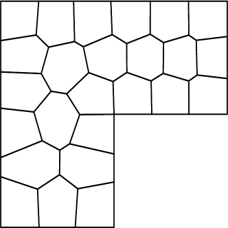
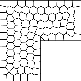
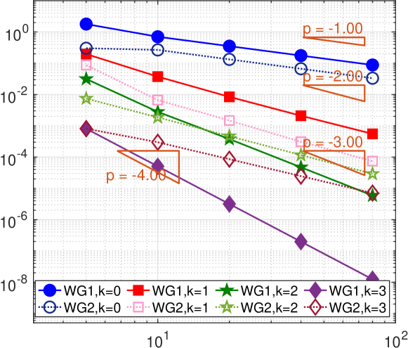
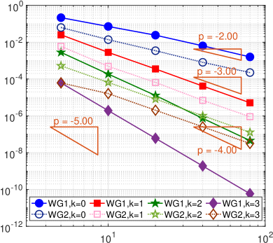
A stabilizer free, pressure robust, and superconvergence weak Galerkin finite element method for the Stokes Equations on polytopal mesh

Lin Mu Department of Mathematics, University of Georgia, Athens, GA 30602 (linmu@uga.edu).    Xiu Ye Department of Mathematics, University of Arkansas at Little Rock, Little Rock, AR 72204 (xxye@ualr.edu). This research was supported in part by National Science Foundation Grant DMS-1620016.    Shangyou Zhang Department of Mathematical Sciences, University of Delaware, Newark, DE 19716 (szhang@udel.edu).
Abstract

In this paper, we propose a new stabilizer free and pressure robust WG method for the Stokes equations with super-convergence on polytopal mesh in the primary velocity-pressure formulation. Convergence rates with one order higher than the optimal-order for velocity in both energy-norm and the L2superscript𝐿2L^{2}-norm and for pressure in L2superscript𝐿2L^{2}-norm are proved in our proposed scheme. The H𝐻H(div)-preserving operator has been constructed based on the polygonal mesh for arbitrary polynomial degrees and employed in the body source assembling to break the locking phenomenon induced by poor mass conservation in the classical discretization. Moreover, the velocity error in our proposed scheme is proved to be independent of pressure and thus confirm the pressure-robustness. For Stokes simulation, our proposed scheme only modifies the body source assembling but remains the same stiffness matrix. Four numerical experiments are conducted to validate the convergence results and robustness.

keywords:
Weak Galerkin, finite element methods, the Stokes equations, super-convergence, pressure-robustness, stabilizer free.
AMS:
Primary, 65N15, 65N30, 76D07; Secondary, 35B45, 35J50

1 Introduction

In this paper, we consider the following viscosity dependent Stokes equations: find velocity 𝐮:Ωd:𝐮Ωsuperscript𝑑{\bf u}:\Omega\to\mathbb{R}^{d} (d = 2 or 3) and pressure: p:Ω:𝑝Ωp:\Omega\to\mathbb{R} such that:

(1) νΔ𝐮+p𝜈Δ𝐮𝑝\displaystyle-\nu\Delta{\bf u}+\nabla p =\displaystyle= 𝐟, in Ω,𝐟 in Ω\displaystyle{\bf f},\text{ in }\Omega,
(2) 𝐮𝐮\displaystyle\nabla\cdot{\bf u} =\displaystyle= 0, in Ω,0 in Ω\displaystyle 0,\text{ in }\Omega,
(3) 𝐮𝐮\displaystyle{\bf u} =\displaystyle= 0, on Ω,0 on Ω\displaystyle 0,\text{ on }\partial\Omega,

where ν>0𝜈0\nu>0 is a constant viscosity parameter and 𝐟𝐋d(Ω)𝐟superscript𝐋𝑑Ω{\bf f}\in{\bf L}^{d}(\Omega) is a given vector field.

The Stokes equation has been widely used in realistic applications. However the classical finite element methods for incompressible Stokes problem are usually not pressure-robust: their velocity error is pressure dependent, shown as follows,

(𝐮𝐮h)Cinf𝐰Vh(𝐮𝐰)+1νinfqQhpq.norm𝐮subscript𝐮𝐶subscriptinfimum𝐰subscript𝑉norm𝐮𝐰1𝜈subscriptinfimum𝑞subscript𝑄norm𝑝𝑞\displaystyle\|\nabla({\bf u}-{\bf u}_{h})\|\leq C\inf_{{\bf w}\in V_{h}}\|\nabla({\bf u}-{\bf w})\|+\frac{1}{\nu}\inf_{q\in Q_{h}}\|p-q\|.

Here Vhsubscript𝑉V_{h} and Qhsubscript𝑄Q_{h} denote the inf-sup stable finite element spaces for velocity and the pressure. We observe that there is a pressure dependent term that can be relatively large for small viscosity ν𝜈\nu. This may cause the locking phenomenon: as small parameters in ν1much-less-than𝜈1\nu\ll 1 will produce large error in velocity; bad approximation in pressure may affect the velocity simulation. To reduce these effects, one would have to increase scheme order and also assume that the pressure is smooth enough.

To remove the pressure dependency in velocity simulation, one has to employ the divergence-free finite element scheme. Nowadays, many divergence-free elements have been developed for two dimensional problems [11, 26] and three dimensional problems [28]. The enrichment of the H(div; ΩΩ\Omega)-conforming elements locally with divergence-free rational shape-functions has been proposed in [12, 13] for two and three dimensional problems. Then by modifying the variational formulation and introduced tangential penalty and thus divergence free schemes are obtained by Cockburn [9] and Wang [27]. Chen proposed to introduce a discrete dual curl operator [8] to achieve divergence free MAC scheme on triangular grids. There are other approaches for dealing with such difficulties by adding grad-div stabilization [23, 24, 14]. In addition, an alternative method to get pressure independent error estimate is introduced recently in [18, 19] by employing a divergence preserving velocity reconstruction operator. In [18], a velocity reconstruction is presented to map discrete divergence free test functions onto exactly divergence free test functions which is applied only on the right hand side for the Stokes equations. This approach was performed for several elements including discontinuous pressure elements [15, 19, 18, 20, 5] and continuous pressure elements [16, 17]. With the help of velocity reconstruction, Linke proposed the pressure-robust schemes leading to a pressure independent velocity error estimate

(𝐮𝐮h)Cinf𝐰Vh(𝐮𝐰).norm𝐮subscript𝐮𝐶subscriptinfimum𝐰subscript𝑉norm𝐮𝐰\displaystyle\|\nabla({\bf u}-{\bf u}_{h})\|\leq C\inf_{{\bf w}\in V_{h}}\|\nabla({\bf u}-{\bf w})\|.

Such schemes are developed on modifying for the existing inf-sup stable schemes to achieve the robustness without compromising the computational accuracy.

Recently, the approximations with flexibility on the polygonal/polyhedral meshes are proposed by many researchers. The features, from handling polygonal meshes and meshes with hanging nodes, include not only weakens the complexity in meshing for the irregular domain but also enhances the efficiency in mesh refining/coarsening in adaptive finite element strategies. Due to features of polygonal finite element framework, there are increasing demands for extending existing numerical schemes to polygonal meshes. Virtual element methods (VEM)[2, 3], mimetic finite difference methods [21], hybrid high order methods (HHO)[25], hybridized discontinuous Galerkin methods (HDG)[10], generalized barycentric coordinates method [7], and weak Galerkin finite element methods (WG)[30] have been developed on these types of meshes for various types of partial differential equations.

In this paper, we focus on developing a new pressure-robust numerical discretization for viscosity dependent Stokes equations on the polygonal meshes. To the best of our knowledge, there are few previous work on the pressure-robust incompressible solver on the polygonal meshes. On triangles/rectangles/tetrahedrons/cubics, such a reconstruction can be defined as to projection into a standard Raviart Thomas or Brezzi Douglas Marini spaces[4]. However, on the polygons, one has to employ the rational bases in the 𝕎0subscript𝕎0\mathbb{CW}_{0}[7] space for constructing the reconstruction operator. Such projection techinique is limited to the lowest order scheme with k=0𝑘0k=0 and convex partitions in the meshes[22]. Another recent work regarding pressure-robust scheme developed by Frerichs[29] was to explore the sub-triangulation and solve the small local Dirichlet boundary value problems for each polygon in the virtual element framework.

In this paper, we propose another H𝐻H(div)-preserving space and propose new projection technique for the velocity reconstruction operator on the polygonal cell and then design the novel pressure-robust based on the weak Galerkin finite element method. The operator is constructed by piecewise RT functions and enforcing extra conditions as (14a)-(14e). The contribution in this work is to show that uniform pressure-robustness, meaning on any mesh, can be attained by the proposed H𝐻H(div,ΩΩ\Omega)-conforming projection ΠhsubscriptΠ\Pi_{h} that preserves the divergence of the test functions 𝐯Vh𝐯subscript𝑉{\bf v}\in V_{h}. Comparing to the existing WG scheme for Stokes equation, our scheme only modifies the body force assembling but remains the same stiffness matrix, and thus achieves the divergence preserving by minimal effort. The techniques designed in this paper can also be integrated into other polygonal finite element methods including HHO, HDG and VEM.

This paper is organized as follows. Brief review regarding basis functions on the polygonal meshes will be presented in Section 2. The discretization is developed in Section 3. Our main results regarding error estimates are stated in Section 4. Section 5 contributes to demonstrate the numerical implementation for velocity reconstruction operator. Section 6 presents several numerical examples for Stokes equations. Finally, this paper is summarized with concluding remarks in Section 7.

2 Preliminary

This section recalls the needed notations, defines the finite element spaces, and introduces the setup of the weak Galerkin finite element methods for the Stokes problem and the velocity reconstruction operator.

2.1 Finite Element Space

Let 𝒯hsubscript𝒯{\cal T}_{h} be a partition of the domain ΩΩ\Omega consisting of polygons in two dimension or polyhedra in three dimension satisfying a set of conditions specified in [31]. Denote by hsubscript{\cal E}_{h} the set of all edges or flat faces in 𝒯hsubscript𝒯{\cal T}_{h}, and let h0=h\Ωsuperscriptsubscript0\subscriptΩ{\cal E}_{h}^{0}={\cal E}_{h}\backslash\partial\Omega be the set of all interior edges or flat faces. For every element T𝒯h𝑇subscript𝒯T\in{\mathcal{T}}_{h}, we denote by hTsubscript𝑇h_{T} its diameter and mesh size h=maxT𝒯hhTsubscript𝑇subscript𝒯subscript𝑇h=\max_{T\in{\mathcal{T}}_{h}}h_{T} for 𝒯hsubscript𝒯{\cal T}_{h}. Let Pk(T)subscript𝑃𝑘𝑇P_{k}(T) consist all the polynomials on T𝑇T with degree no greater than k𝑘k.

For k0𝑘0k\geq 0 and given 𝒯hsubscript𝒯{\mathcal{T}}_{h}, for T𝒯h𝑇subscript𝒯T\in{\mathcal{T}}_{h} define two finite element spaces for velocity

(4) Vhsubscript𝑉\displaystyle V_{h} =\displaystyle= {𝐯={𝐯0,𝐯b}:𝐯0|T[Pk(T)]d,𝐯b|e[Pk(e)]d,eT}.conditional-set𝐯subscript𝐯0subscript𝐯𝑏formulae-sequenceevaluated-atsubscript𝐯0𝑇superscriptdelimited-[]subscript𝑃𝑘𝑇𝑑formulae-sequenceevaluated-atsubscript𝐯𝑏𝑒superscriptdelimited-[]subscript𝑃𝑘𝑒𝑑𝑒𝑇\displaystyle\left\{{\bf v}=\{{\bf v}_{0},{\bf v}_{b}\}:\ {\bf v}_{0}|_{T}\in[P_{k}(T)]^{d},\;{\bf v}_{b}|_{e}\in[P_{k}(e)]^{d},e\subset{\partial T}\right\}.

and for pressure

(5) Wh={wL02(Ω):w|TPk(T)}.subscript𝑊conditional-set𝑤superscriptsubscript𝐿02Ωevaluated-at𝑤𝑇subscript𝑃𝑘𝑇W_{h}=\left\{w\in L_{0}^{2}(\Omega):\ w|_{T}\in P_{k}(T)\right\}.

It is noted that the 𝐯bsubscript𝐯𝑏{\bf v}_{b} has a single value on the faces of triangulation. Let Vh0superscriptsubscript𝑉0V_{h}^{0} be a subspace of Vhsubscript𝑉V_{h} consisting of functions with vanishing boundary value.

The space H(div;Ω)𝐻divΩH(\operatorname{div};\Omega) is defined as the set of vector-valued functions on ΩΩ\Omega which, together with their divergence, are square integrable; i.e.,

H(div;Ω)={𝐯[L2(Ω)]d:𝐯L2(Ω)}.𝐻divΩconditional-set𝐯superscriptdelimited-[]superscript𝐿2Ω𝑑𝐯superscript𝐿2ΩH(\operatorname{div};\Omega)=\left\{{\bf v}\in[L^{2}(\Omega)]^{d}:\;\nabla\cdot{\bf v}\in L^{2}(\Omega)\right\}.

In order to introduce the local finite element space to mimic the H(div;Ω)𝐻divΩH(\operatorname{div};\Omega). For any T𝒯h𝑇subscript𝒯T\in{\mathcal{T}}_{h}, it can be divided in to a set of disjoint triangles Tisubscript𝑇𝑖T_{i} with T=Ti𝑇subscript𝑇𝑖T=\cup T_{i}. We define a local space Λk(T)subscriptΛ𝑘𝑇\Lambda_{k}(T)([32])

(6) Λk(T)={𝐯H(div,T):𝐯|TiRTk(Ti),𝐯Pk(T)},subscriptΛ𝑘𝑇conditional-set𝐯𝐻div𝑇formulae-sequenceevaluated-at𝐯subscript𝑇𝑖𝑅subscript𝑇𝑘subscript𝑇𝑖𝐯subscript𝑃𝑘𝑇\displaystyle\Lambda_{k}(T)=\{{\bf v}\in H(\operatorname{div},T):\ {\bf v}|_{T_{i}}\in RT_{k}(T_{i}),\;\;\nabla\cdot{\bf v}\in P_{k}(T)\},

and a global space V~hsubscript~𝑉\tilde{V}_{h} as

(7) V~h={𝐯H(div,Ω):𝐯|TΛk(T),T𝒯h}.subscript~𝑉conditional-set𝐯𝐻divΩformulae-sequenceevaluated-at𝐯𝑇subscriptΛ𝑘𝑇𝑇subscript𝒯\displaystyle\tilde{V}_{h}=\{{\bf v}\in H(\operatorname{div},\Omega):\ {\bf v}|_{T}\in\Lambda_{k}(T),\;T\in{\mathcal{T}}_{h}\}.

Then we define a space IΛh(T)IsubscriptΛ𝑇\mathrm{I}\Lambda_{h}(T) for the approximation of weak gradient on each element T𝑇T as

IΛk(T)={𝝍[H(div;T)]d:\displaystyle\mathrm{I}\Lambda_{k}(T)=\{{\bm{\psi}}\in[H(\operatorname{div};T)]^{d}: 𝝍|Ti[RTk(Ti)]d,𝝍[Pk(T)]d,formulae-sequenceevaluated-at𝝍subscript𝑇𝑖superscriptdelimited-[]𝑅subscript𝑇𝑘subscript𝑇𝑖𝑑𝝍superscriptdelimited-[]subscript𝑃𝑘𝑇𝑑\displaystyle\ {\bm{\psi}}|_{T_{i}}\in[RT_{k}(T_{i})]^{d},\;\;\nabla\cdot{\bm{\psi}}\in[P_{k}(T)]^{d},
𝝍𝐧|e[Pk(e)]d,eT},\displaystyle{\bm{\psi}}\cdot{\bf n}|_{e}\in[P_{k}(e)]^{d},\;e\subset{\partial T}\},

where RTk(Ti)𝑅subscript𝑇𝑘subscript𝑇𝑖RT_{k}(T_{i}) is the usual Raviart-Thomas element [6] of order k𝑘k.

Definition 1.

For a function 𝐯Vh𝐯subscript𝑉{\bf v}\in V_{h}, its weak gradient w𝐯subscript𝑤𝐯\nabla_{w}{\bf v} is a piecewise polynomial such that w𝐯|TIΛk(T)evaluated-atsubscript𝑤𝐯𝑇IsubscriptΛ𝑘𝑇\nabla_{w}{\bf v}|_{T}\in\mathrm{I}\Lambda_{k}(T) and satisfies the following equation,

(9) (w𝐯,𝝉)T=(𝐯0,𝝉)T+𝐯b,τ𝐧T𝝉IΛk(T).formulae-sequencesubscriptsubscript𝑤𝐯𝝉𝑇subscriptsubscript𝐯0𝝉𝑇subscriptsubscript𝐯𝑏𝜏𝐧𝑇for-all𝝉IsubscriptΛ𝑘𝑇(\nabla_{w}{\bf v},\ \bm{\tau})_{T}=-({\bf v}_{0},\ \nabla\cdot\bm{\tau})_{T}+{\langle}{\bf v}_{b},\ \tau\cdot{\bf n}{\rangle}_{\partial T}\quad\forall\bm{\tau}\in\mathrm{I}\Lambda_{k}(T).
Definition 2.1.

For a function 𝐯Vh𝐯subscript𝑉{\bf v}\in V_{h}, its weak divergence w𝐯subscript𝑤𝐯\nabla_{w}\cdot{\bf v} is a piecewise polynomial such that w𝐯|TPk(T)evaluated-atsubscript𝑤𝐯𝑇subscript𝑃𝑘𝑇\nabla_{w}\cdot{\bf v}|_{T}\in P_{k}(T) and satisfies the following equation,

(10) (w𝐯,τ)T=(𝐯0,τ)T+𝐯b𝐧,τTτPk(T).formulae-sequencesubscriptsubscript𝑤𝐯𝜏𝑇subscriptsubscript𝐯0𝜏𝑇subscriptsubscript𝐯𝑏𝐧𝜏𝑇for-all𝜏subscript𝑃𝑘𝑇(\nabla_{w}\cdot{\bf v},\ \tau)_{T}=-({\bf v}_{0},\ \nabla\tau)_{T}+{\langle}{\bf v}_{b}\cdot{\bf n},\ \tau{\rangle}_{\partial T}\quad\forall\tau\in P_{k}(T).
Lemma 2.

For 𝛕[H(div;Ω)]d𝛕superscriptdelimited-[]𝐻divΩ𝑑\bm{\tau}\in[H(\operatorname{div};\Omega)]^{d}, there exists a projection πhsubscript𝜋\pi_{h} with πh𝛕[H(div;Ω)]dsubscript𝜋𝛕superscriptdelimited-[]𝐻divΩ𝑑\pi_{h}\bm{\tau}\in[H(\operatorname{div};\Omega)]^{d} satisfying πh𝛕|TIΛk(T)evaluated-atsubscript𝜋𝛕𝑇IsubscriptΛ𝑘𝑇\pi_{h}\bm{\tau}|_{T}\in\mathrm{I}\Lambda_{k}(T) and

(11) (πh𝝉,σ)Tsubscriptsubscript𝜋𝝉𝜎𝑇\displaystyle(\pi_{h}\bm{\tau},\;\sigma)_{T} =\displaystyle= (𝝉,σ)Tσ[Pk1(T)]d×d,subscript𝝉𝜎𝑇for-all𝜎superscriptdelimited-[]subscript𝑃𝑘1𝑇𝑑𝑑\displaystyle(\bm{\tau},\;\sigma)_{T}\quad\forall\sigma\in[P_{k-1}(T)]^{d\times d},
(12) πh𝝉𝐧,𝐪esubscriptsubscript𝜋𝝉𝐧𝐪𝑒\displaystyle{\langle}\pi_{h}\bm{\tau}\cdot{\bf n},\;{\bf q}{\rangle}_{e} =\displaystyle= 𝐯𝐧,𝐪e𝐪[Pk(e)]d,eT,formulae-sequencesubscript𝐯𝐧𝐪𝑒for-all𝐪superscriptdelimited-[]subscript𝑃𝑘𝑒𝑑𝑒𝑇\displaystyle{\langle}{\bf v}\cdot{\bf n},\;{\bf q}{\rangle}_{e}\quad\forall{\bf q}\in[P_{k}(e)]^{d},e\subset{\partial T},
(13) πh𝝉𝝉normsubscript𝜋𝝉𝝉\displaystyle\|\pi_{h}\bm{\tau}-\bm{\tau}\| \displaystyle\leq Chk+1|𝝉|k+1.𝐶superscript𝑘1subscript𝝉𝑘1\displaystyle Ch^{k+1}|\bm{\tau}|_{k+1}.

The proof of the above lemma can be found in [33].

2.2 Velocity Reconstruction Operator

This section shall describe the velocity reconstruction operator that is H(div,ΩΩ\Omega)-conforming and preserves the divergence of the weak functions for all polygons T𝒯h𝑇subscript𝒯T\in\mathcal{T}_{h}. The main idea is to employ a sub-triangulation of each polygon and use the piecewise RT(Tj)k{}_{k}(T_{j}) functions with some extra constraints. Here we shall cite the construction of the finite element space Λk(T)subscriptΛ𝑘𝑇\Lambda_{k}(T), which has been studies in [32].

Assume no additional inner vertex/edges is introduced in subdividing a polygon T𝑇T into n𝑛n triangles {Ti}i=1nsuperscriptsubscriptsubscript𝑇𝑖𝑖1𝑛\{T_{i}\}_{i=1}^{n}. Thus, we have n1𝑛1n-1 internal edges which separate T𝑇T into n𝑛n parts. In the 2D setting, we are ready to define the velocity reconstruction operator as below: For 𝐯={𝐯0,𝐯b}Vh𝐯subscript𝐯0subscript𝐯𝑏subscript𝑉{\bf v}=\{{\bf v}_{0},{\bf v}_{b}\}\in V_{h}, the projection Πh:VhV~h:subscriptΠsubscript𝑉subscript~𝑉\Pi_{h}:V_{h}\to\tilde{V}_{h} is defined such that

(14a) eiT(Πh𝐯𝐧i)pk𝑑s=eiT(𝐯b𝐧i)pk𝑑s,pkPk(ei)formulae-sequencesubscriptsubscript𝑒𝑖𝑇subscriptΠ𝐯subscript𝐧𝑖subscript𝑝𝑘differential-d𝑠subscriptsubscript𝑒𝑖𝑇subscript𝐯𝑏subscript𝐧𝑖subscript𝑝𝑘differential-d𝑠for-allsubscript𝑝𝑘subscript𝑃𝑘subscript𝑒𝑖\displaystyle\int_{e_{i}\subset\partial T}(\Pi_{h}{\bf v}\cdot{\bf n}_{i})p_{k}ds=\int_{e_{i}\subset\partial T}({\bf v}_{b}\cdot{\bf n}_{i})p_{k}ds,\ \forall p_{k}\in P_{k}(e_{i})
(14b) TΠh𝐯𝐧1pk1𝑑𝐱=T𝐯0𝐧1pk1𝑑𝐱,pk1Pk1(T),formulae-sequencesubscript𝑇subscriptΠ𝐯subscript𝐧1subscript𝑝𝑘1differential-d𝐱subscript𝑇subscript𝐯0subscript𝐧1subscript𝑝𝑘1differential-d𝐱for-allsubscript𝑝𝑘1subscript𝑃𝑘1𝑇\displaystyle\int_{T}\Pi_{h}{\bf v}\cdot{\bf n}_{1}p_{k-1}d{\bf x}=\int_{T}{\bf v}_{0}\cdot{\bf n}_{1}p_{k-1}d{\bf x},\ \forall p_{k-1}\in P_{k-1}(T),
(14c) TiΠh𝐯𝐧2pk1𝑑𝐱=Ti𝐯0𝐧2pk1,pk1Pk1(Ti),i=1,,n,formulae-sequencesubscriptsubscript𝑇𝑖subscriptΠ𝐯subscript𝐧2subscript𝑝𝑘1differential-d𝐱subscriptsubscript𝑇𝑖subscript𝐯0subscript𝐧2subscript𝑝𝑘1formulae-sequencefor-allsubscript𝑝𝑘1subscript𝑃𝑘1subscript𝑇𝑖𝑖1𝑛\displaystyle\int_{T_{i}}\Pi_{h}{\bf v}\cdot{\bf n}_{2}p_{k-1}d{\bf x}=\int_{T_{i}}{\bf v}_{0}\cdot{\bf n}_{2}p_{k-1},\ \forall p_{k-1}\in P_{k-1}(T_{i}),\ i=1,\cdots,n,
(14d) ejT0[[Πh𝐯]]𝐧jpk𝑑s=0,pkPk(ej),formulae-sequencesubscriptsubscript𝑒𝑗superscript𝑇0delimited-[]delimited-[]subscriptΠ𝐯subscript𝐧𝑗subscript𝑝𝑘differential-d𝑠0for-allsubscript𝑝𝑘subscript𝑃𝑘subscript𝑒𝑗\displaystyle\int_{e_{j}\subset T^{0}}{[\![}\Pi_{h}{\bf v}{]\!]}\cdot{\bf n}_{j}p_{k}ds=0,\ \forall p_{k}\in P_{k}(e_{j}),
(14e) T1(Πh𝐯|TiΠh𝐯|T1)pk𝑑𝐱=0,pkPk(T1),i=2,,n,formulae-sequencesubscriptsubscript𝑇1evaluated-atsubscriptΠ𝐯subscript𝑇𝑖evaluated-atsubscriptΠ𝐯subscript𝑇1subscript𝑝𝑘differential-d𝐱0formulae-sequencefor-allsubscript𝑝𝑘subscript𝑃𝑘subscript𝑇1𝑖2𝑛\displaystyle\int_{T_{1}}\nabla\cdot(\Pi_{h}{\bf v}|_{T_{i}}-\Pi_{h}{\bf v}|_{T_{1}})p_{k}d{\bf x}=0,\ \forall p_{k}\in P_{k}(T_{1}),\ i=2,\dots,n,

where eijsubscript𝑒𝑖𝑗e_{ij} is the j𝑗j-th edge of Tjsubscript𝑇𝑗T_{j} with a fixed normal vector 𝐧ijsubscript𝐧𝑖𝑗{\bf n}_{ij}, 𝐧1subscript𝐧1{\bf n}_{1} is a unite vector not parallel to any internal face normal 𝐧ijsubscript𝐧𝑖𝑗{\bf n}_{ij}, (𝐧1,𝐧2subscript𝐧1subscript𝐧2{\bf n}_{1},{\bf n}_{2}) forms a right-hand orthonormal system, [[]]delimited-[]delimited-[]{[\![}\cdot{]\!]} denotes the jump on a edge, Πh𝐯|Tievaluated-atsubscriptΠ𝐯subscript𝑇𝑖\Pi_{h}{\bf v}|_{T_{i}} is understood as a polynomial vector which can be used on another triangle T1.subscript𝑇1T_{1}. When k=0𝑘0k=0, the conditions (14b)-(14c) are not needed.

Lemma 3.

For 𝐯={𝐯0,𝐯b}Vh𝐯subscript𝐯0subscript𝐯𝑏subscript𝑉{\bf v}=\{{\bf v}_{0},{\bf v}_{b}\}\in V_{h}, there exists a projection Πh:VhV~h:subscriptΠsubscript𝑉subscript~𝑉\Pi_{h}:V_{h}\to\tilde{V}_{h} such that

(15) (Πh𝐯,𝐪)TsubscriptsubscriptΠ𝐯𝐪𝑇\displaystyle(\Pi_{h}{\bf v},{\bf q})_{T} =\displaystyle= (𝐯0,𝐪)T𝐪[Pk1(T)]d,subscriptsubscript𝐯0𝐪𝑇for-all𝐪superscriptdelimited-[]subscript𝑃𝑘1𝑇𝑑\displaystyle({\bf v}_{0},{\bf q})_{T}\quad\forall{\bf q}\in[P_{k-1}(T)]^{d},
(16) Πh𝐯𝐧,wesubscriptsubscriptΠ𝐯𝐧𝑤𝑒\displaystyle{\langle}\Pi_{h}{\bf v}\cdot{\bf n},\;w{\rangle}_{e} =\displaystyle= 𝐯b𝐧,wewPk(e),eT,formulae-sequencesubscriptsubscript𝐯𝑏𝐧𝑤𝑒for-all𝑤subscript𝑃𝑘𝑒𝑒𝑇\displaystyle{\langle}{\bf v}_{b}\cdot{\bf n},\;w{\rangle}_{e}\quad\forall w\in P_{k}(e),\ e\subset{\partial T},
(17) Πh𝐯𝐯0normsubscriptΠ𝐯subscript𝐯0\displaystyle\|\Pi_{h}{\bf v}-{\bf v}_{0}\| \displaystyle\leq C(T𝒯hhT𝐯0𝐯bT2)1/2.𝐶superscriptsubscript𝑇subscript𝒯subscript𝑇superscriptsubscriptnormsubscript𝐯0subscript𝐯𝑏𝑇212\displaystyle C(\sum_{T\in{\mathcal{T}}_{h}}h_{T}\|{\bf v}_{0}-{\bf v}_{b}\|_{{\partial T}}^{2})^{1/2}.
Proof.

A projection operator ΠhsubscriptΠ\Pi_{h} is defined in [32] for smooth functions satisfying (15)-(16). Then by the definition of weak divergence w𝐯subscript𝑤𝐯\nabla_{w}\cdot{\bf v} For any 𝐯={𝐯0,𝐯b}𝐯subscript𝐯0subscript𝐯𝑏{\bf v}=\{{\bf v}_{0},{\bf v}_{b}\}, we can select any smooth function 𝐮𝐇1(Ω)𝐮superscript𝐇1Ω{\bf u}\in\mathbf{H}^{1}(\Omega) such that Qh𝐮=𝐯subscript𝑄𝐮𝐯Q_{h}{\bf u}={\bf v}, i.e., Q0𝐮=𝐯0subscript𝑄0𝐮subscript𝐯0Q_{0}{\bf u}={\bf v}_{0} and Qb𝐮=𝐯bsubscript𝑄𝑏𝐮subscript𝐯𝑏Q_{b}{\bf u}={\bf v}_{b}. We note that Qhsubscript𝑄Q_{h} is an on-to mapping from 𝐇1(Ω)superscript𝐇1Ω\mathbf{H}^{1}(\Omega) to Vhsubscript𝑉V_{h}. Now we define

Πh𝐯=Πh𝐮.subscriptΠ𝐯subscriptΠ𝐮\displaystyle\Pi_{h}{\bf v}=\Pi_{h}{\bf u}.

It follows that

(Πh𝐯,𝐪)TsubscriptsubscriptΠ𝐯𝐪𝑇\displaystyle(\Pi_{h}{\bf v},{\bf q})_{T} =(Πh𝐮,𝐪)T=(Q0𝐮,𝐪)T=(𝐯0,𝐪)TabsentsubscriptsubscriptΠ𝐮𝐪𝑇subscriptsubscript𝑄0𝐮𝐪𝑇subscriptsubscript𝐯0𝐪𝑇\displaystyle=(\Pi_{h}{\bf u},{\bf q})_{T}=(Q_{0}{\bf u},{\bf q})_{T}=({\bf v}_{0},{\bf q})_{T}

for all 𝐪[Pk1(T)]d𝐪superscriptdelimited-[]subscript𝑃𝑘1𝑇𝑑{\bf q}\in[P_{k-1}(T)]^{d}. For the same reason, we have

Πh𝐯𝐧,wesubscriptsubscriptΠ𝐯𝐧𝑤𝑒\displaystyle{\langle}\Pi_{h}{\bf v}\cdot{\bf n},\;w{\rangle}_{e} =Πh𝐮𝐧,we=𝐮𝐧,we=Qb𝐮𝐧,we=𝐯b𝐧,weabsentsubscriptsubscriptΠ𝐮𝐧𝑤𝑒subscript𝐮𝐧𝑤𝑒subscriptsubscript𝑄𝑏𝐮𝐧𝑤𝑒subscriptsubscript𝐯𝑏𝐧𝑤𝑒\displaystyle={\langle}\Pi_{h}{\bf u}\cdot{\bf n},\;w{\rangle}_{e}={\langle}{\bf u}\cdot{\bf n},\;w{\rangle}_{e}={\langle}Q_{b}{\bf u}\cdot{\bf n},\;w{\rangle}_{e}={\langle}{\bf v}_{b}\cdot{\bf n},\;w{\rangle}_{e}

for all wPk(e),eTformulae-sequence𝑤subscript𝑃𝑘𝑒𝑒𝑇w\in P_{k}(e),\ e\subset{\partial T}. From interpolation/projection data and scaling argument, we have

Πh𝐮TsubscriptnormsubscriptΠ𝐮𝑇\displaystyle\|\Pi_{h}\mathbf{u}\|_{T} C(ΠTk1𝐮0+hTQb𝐮𝐧T),absent𝐶subscriptnormsuperscriptsubscriptΠ𝑇𝑘1𝐮0subscript𝑇subscriptnormsubscript𝑄𝑏𝐮𝐧𝑇\displaystyle\leq C(\|\Pi_{T}^{k-1}\mathbf{u}\|_{0}+h_{T}\|Q_{b}{\bf u}\cdot{\bf n}\|_{\partial T}),

where ΠTk1superscriptsubscriptΠ𝑇𝑘1\Pi_{T}^{k-1} is the L2superscript𝐿2L^{2}-projection to [Pk1(T)]dsuperscriptdelimited-[]subscript𝑃𝑘1𝑇𝑑[P_{k-1}(T)]^{d}. Finally we derive

Πh𝐯𝐯02superscriptnormsubscriptΠ𝐯subscript𝐯02\displaystyle\|\Pi_{h}{\bf v}-{\bf v}_{0}\|^{2} =Πh(𝐮𝐯0)2absentsuperscriptnormsubscriptΠ𝐮subscript𝐯02\displaystyle=\|\Pi_{h}({\bf u}-{\bf v}_{0})\|^{2}
CT𝒯h(ΠTk1(Q0𝐮𝐯0)T2+hT2Qb(𝐮𝐯0)𝐧T2)absent𝐶subscript𝑇subscript𝒯superscriptsubscriptnormsuperscriptsubscriptΠ𝑇𝑘1subscript𝑄0𝐮subscript𝐯0𝑇2superscriptsubscript𝑇2superscriptsubscriptnormsubscript𝑄𝑏𝐮subscript𝐯0𝐧𝑇2\displaystyle\leq C\sum_{T\in{\mathcal{T}}_{h}}\Big{(}\|\Pi_{T}^{k-1}(Q_{0}{\bf u}-{\bf v}_{0})\|_{T}^{2}+h_{T}^{2}\|Q_{b}({\bf u}-{\bf v}_{0})\cdot{\bf n}\|_{\partial T}^{2}\Big{)}
=ChT2T𝒯h(𝐯b𝐯0)𝐧T2absent𝐶superscriptsubscript𝑇2subscript𝑇subscript𝒯superscriptsubscriptnormsubscript𝐯𝑏subscript𝐯0𝐧𝑇2\displaystyle=Ch_{T}^{2}\sum_{T\in{\mathcal{T}}_{h}}\|({\bf v}_{b}-{\bf v}_{0})\cdot{\bf n}\|_{\partial T}^{2}
ChT2T𝒯h𝐯b𝐯0T2,absent𝐶superscriptsubscript𝑇2subscript𝑇subscript𝒯superscriptsubscriptnormsubscript𝐯𝑏subscript𝐯0𝑇2\displaystyle\leq Ch_{T}^{2}\sum_{T\in{\mathcal{T}}_{h}}\|{\bf v}_{b}-{\bf v}_{0}\|_{\partial T}^{2},

and thus complete the proof. ∎

3 Numerical Scheme

This section contributes to develop the new weak Galerkin finite element scheme and investigate the well-posedness for the proposed scheme.

3.1 Finite Element Scheme

We start this section by introducing the following simple WG finite element scheme without stabilizers.

Weak Galerkin Algorithm 1.

Our new numerical approximation for (1)-(3) is seeking 𝐮hVh0subscript𝐮superscriptsubscript𝑉0{\bf u}_{h}\in V_{h}^{0} and phWhsubscript𝑝subscript𝑊p_{h}\in W_{h} such that for all 𝐯Vh0𝐯superscriptsubscript𝑉0{\bf v}\in V_{h}^{0} and wWh𝑤subscript𝑊w\in W_{h},

(18) (νw𝐮h,w𝐯)(w𝐯,ph)𝜈subscript𝑤subscript𝐮subscript𝑤𝐯subscript𝑤𝐯subscript𝑝\displaystyle(\nu\nabla_{w}{\bf u}_{h},\ \nabla_{w}{\bf v})-(\nabla_{w}\cdot{\bf v},\;p_{h}) =\displaystyle= (f,Πh𝐯),𝑓subscriptΠ𝐯\displaystyle(f,\;\Pi_{h}{\bf v}),
(19) (w𝐮h,w)subscript𝑤subscript𝐮𝑤\displaystyle(\nabla_{w}\cdot{\bf u}_{h},\;w) =\displaystyle= 0.0\displaystyle 0.

In comparison, we shall also cite the following stabilizer free weak Galerkin finite element scheme in [33].

Weak Galerkin Algorithm 2.

[33]. A numerical approximation for (1)-(3) is seeking 𝐮hVhsubscript𝐮subscript𝑉{\bf u}_{h}\in V_{h} and phWhsubscript𝑝subscript𝑊p_{h}\in W_{h} such that for all 𝐯Vh0𝐯superscriptsubscript𝑉0{\bf v}\in V_{h}^{0} and wWh𝑤subscript𝑊w\in W_{h},

(20) (νw𝐮h,w𝐯)(w𝐯,ph)𝜈subscript𝑤subscript𝐮subscript𝑤𝐯subscript𝑤𝐯subscript𝑝\displaystyle(\nu\nabla_{w}{\bf u}_{h},\nabla_{w}{\bf v})-(\nabla_{w}\cdot{\bf v},p_{h}) =\displaystyle= (𝐟,𝐯),𝐟𝐯\displaystyle({\bf f},{\bf v}),
(21) (w𝐮h,w)subscript𝑤subscript𝐮𝑤\displaystyle(\nabla_{w}\cdot{\bf u}_{h},w) =\displaystyle= 0.0\displaystyle 0.
Remark 1.

It is noted that Algorithm 1 and Algorithm 2 share the same stiffness matrix.

3.2 Well Posedness

Let Q0subscript𝑄0Q_{0} and Qbsubscript𝑄𝑏Q_{b} be the two element-wise defined L2superscript𝐿2L^{2} projections onto [Pk(T)]dsuperscriptdelimited-[]subscript𝑃𝑘𝑇𝑑[P_{k}(T)]^{d} and [Pk(e)]dsuperscriptdelimited-[]subscript𝑃𝑘𝑒𝑑[P_{k}(e)]^{d} with eT𝑒𝑇e\subset\partial T on T𝑇T respectively for velocity. Denote by 𝒬hsubscript𝒬\mathcal{Q}_{h} the element-wise defined L2superscript𝐿2L^{2} projection onto Pk(T)subscript𝑃𝑘𝑇P_{k}(T) on each element T𝑇T for pressure variable. Let hsubscript{\mathbb{Q}}_{h} be the element-wise defined L2superscript𝐿2L^{2} projection onto IΛk(T)IsubscriptΛ𝑘𝑇\mathrm{I}\Lambda_{k}(T) on each element T𝑇T for the proximation of 𝐮𝐮\nabla{\bf u}. Finally we define Qh𝐮={Q0𝐮,Qb𝐮}Vhsubscript𝑄𝐮subscript𝑄0𝐮subscript𝑄𝑏𝐮subscript𝑉Q_{h}{\bf u}=\{Q_{0}{\bf u},Q_{b}{\bf u}\}\in V_{h} for the true solution 𝐮𝐮{\bf u}. The following lemma reveal commutative properties for weak gradient wsubscript𝑤\nabla_{w} and weak divergence w\nabla_{w}\cdot.

Lemma 4.

Let ϕ[H01(Ω)]dbold-ϕsuperscriptdelimited-[]superscriptsubscript𝐻01Ω𝑑\bm{\phi}\in[H_{0}^{1}(\Omega)]^{d}, then on T𝒯h𝑇subscript𝒯T\in{\mathcal{T}}_{h}

(22) wQhϕsubscript𝑤subscript𝑄bold-italic-ϕ\displaystyle\nabla_{w}Q_{h}\bm{\phi} =\displaystyle= hϕ,subscriptbold-italic-ϕ\displaystyle{\mathbb{Q}}_{h}\nabla\bm{\phi},
(23) wQhϕsubscript𝑤subscript𝑄bold-italic-ϕ\displaystyle\nabla_{w}\cdot Q_{h}\bm{\phi} =\displaystyle= 𝒬hϕ.subscript𝒬bold-italic-ϕ\displaystyle\mathcal{Q}_{h}\nabla\cdot\bm{\phi}.
Proof.

Using (9) and integration by parts, we have that for any τΛk(T)𝜏subscriptΛ𝑘𝑇\tau\in\Lambda_{k}(T)

(wQhϕ,τ)Tsubscriptsubscript𝑤subscript𝑄bold-italic-ϕ𝜏𝑇\displaystyle(\nabla_{w}Q_{h}\bm{\phi},\tau)_{T} =\displaystyle= (Q0ϕ,τ)T+Qbϕ,τ𝐧Tsubscriptsubscript𝑄0bold-italic-ϕ𝜏𝑇subscriptsubscript𝑄𝑏bold-italic-ϕ𝜏𝐧𝑇\displaystyle-(Q_{0}\bm{\phi},\nabla\cdot\tau)_{T}+\langle Q_{b}\bm{\phi},\tau\cdot{\bf n}\rangle_{{\partial T}}
=\displaystyle= (ϕ,τ)T+ϕ,τ𝐧Tsubscriptbold-italic-ϕ𝜏𝑇subscriptbold-italic-ϕ𝜏𝐧𝑇\displaystyle-(\bm{\phi},\nabla\cdot\tau)_{T}+\langle\bm{\phi},\tau\cdot{\bf n}\rangle_{{\partial T}}
=\displaystyle= (ϕ,τ)T=(hϕ,τ)T.subscriptbold-italic-ϕ𝜏𝑇subscriptsubscriptbold-italic-ϕ𝜏𝑇\displaystyle(\nabla\bm{\phi},\tau)_{T}=({\mathbb{Q}}_{h}\nabla\bm{\phi},\tau)_{T}.

The equation above proves the identity (22).

It follows from (10) and integration by parts that for any wPk(T)𝑤subscript𝑃𝑘𝑇w\in P_{k}(T)

(wQhϕ,w)Tsubscriptsubscript𝑤subscript𝑄bold-italic-ϕ𝑤𝑇\displaystyle(\nabla_{w}\cdot Q_{h}\bm{\phi},w)_{T} =\displaystyle= (Q0ϕ,w)T+Qbϕ𝐧,wTsubscriptsubscript𝑄0bold-italic-ϕ𝑤𝑇subscriptsubscript𝑄𝑏bold-italic-ϕ𝐧𝑤𝑇\displaystyle-(Q_{0}\bm{\phi},\nabla w)_{T}+\langle Q_{b}\bm{\phi}\cdot{\bf n},w\rangle_{{\partial T}}
=\displaystyle= (ϕ,w)T+ϕ𝐧,wTsubscriptbold-italic-ϕ𝑤𝑇subscriptbold-italic-ϕ𝐧𝑤𝑇\displaystyle-(\bm{\phi},\nabla w)_{T}+\langle\bm{\phi}\cdot{\bf n},w\rangle_{{\partial T}}
=\displaystyle= (ϕ,w)T=(𝒬hϕ,w)T,subscriptbold-italic-ϕ𝑤𝑇subscriptsubscript𝒬bold-italic-ϕ𝑤𝑇\displaystyle(\nabla\cdot\bm{\phi},w)_{T}=(\mathcal{Q}_{h}\nabla\cdot\bm{\phi},w)_{T},

which proves (23). ∎

For any function φH1(T)𝜑superscript𝐻1𝑇\varphi\in H^{1}(T), the following trace inequality holds true (see [31] for details):

(24) φe2C(hT1φT2+hTφT2).superscriptsubscriptnorm𝜑𝑒2𝐶superscriptsubscript𝑇1superscriptsubscriptnorm𝜑𝑇2subscript𝑇superscriptsubscriptnorm𝜑𝑇2\|\varphi\|_{e}^{2}\leq C\left(h_{T}^{-1}\|\varphi\|_{T}^{2}+h_{T}\|\nabla\varphi\|_{T}^{2}\right).

We introduce two semi-norms |𝐯|norm𝐯{|||}{\bf v}{|||} and 𝐯1,hsubscriptnorm𝐯1\|{\bf v}\|_{1,h} for any 𝐯Vh𝐯subscript𝑉{\bf v}\in V_{h} as follows:

(25) |𝐯|2superscriptnorm𝐯2\displaystyle{|||}{\bf v}{|||}^{2} =\displaystyle= T𝒯h(w𝐯,w𝐯)T,subscript𝑇subscript𝒯subscriptsubscript𝑤𝐯subscript𝑤𝐯𝑇\displaystyle\sum_{T\in{\mathcal{T}}_{h}}(\nabla_{w}{\bf v},\nabla_{w}{\bf v})_{T},
(26) 𝐯1,h2superscriptsubscriptnorm𝐯12\displaystyle\|{\bf v}\|_{1,h}^{2} =\displaystyle= T𝒯h𝐯0T2+T𝒯hhT1𝐯0𝐯bT2.subscript𝑇subscript𝒯superscriptsubscriptnormsubscript𝐯0𝑇2subscript𝑇subscript𝒯superscriptsubscript𝑇1superscriptsubscriptnormsubscript𝐯0subscript𝐯𝑏𝑇2\displaystyle\sum_{T\in{\mathcal{T}}_{h}}\|\nabla{\bf v}_{0}\|_{T}^{2}+\sum_{T\in{\mathcal{T}}_{h}}h_{T}^{-1}\|{\bf v}_{0}-{\bf v}_{b}\|_{{\partial T}}^{2}.

It is easy to see that 𝐯1,hsubscriptnorm𝐯1\|{\bf v}\|_{1,h} defines a norm in Vh0superscriptsubscript𝑉0V_{h}^{0}. Next we will show that ||||||{|||}\cdot{|||} also defines a norm in Vh0superscriptsubscript𝑉0V_{h}^{0} by proving the equivalence of ||||||{|||}\cdot{|||} and 1,h\|\cdot\|_{1,h} in Vhsubscript𝑉V_{h}.

The following norm equivalence has been proved in [32] for each component of 𝐯𝐯{\bf v},

(27) C1𝐯1,h|𝐯|C2𝐯1,h𝐯Vh.formulae-sequencesubscript𝐶1subscriptnorm𝐯1norm𝐯subscript𝐶2subscriptnorm𝐯1for-all𝐯subscript𝑉C_{1}\|{\bf v}\|_{1,h}\leq{|||}{\bf v}{|||}\leq C_{2}\|{\bf v}\|_{1,h}\quad\forall{\bf v}\in V_{h}.

The inf-sup condition for the finite element formulation (18)-(19) is derived in the following lemma.

Lemma 5.

There exists a positive constant β𝛽\beta independent of hh such that for all ρWh𝜌subscript𝑊\rho\in W_{h},

(28) sup𝐯Vh(w𝐯,ρ)|𝐯|βρ.subscriptsupremum𝐯subscript𝑉subscript𝑤𝐯𝜌norm𝐯𝛽norm𝜌\sup_{{\bf v}\in V_{h}}\frac{(\nabla_{w}\cdot{\bf v},\rho)}{{|||}{\bf v}{|||}}\geq\beta\|\rho\|.
Lemma 6.

The weak Galerkin method (18)-(19) has a unique solution.

The proofs for Lemma 5 and Lemma 6 are similar to the proofs in [33].

4 Main Results

This section contributes to the pressure-robust estimates for our proposed numerical scheme (18)-(19).

4.1 Error Equations

In this section, we derive the equations that the errors satisfy. Let 𝐞h=Qh𝐮𝐮hsubscript𝐞subscript𝑄𝐮subscript𝐮{\bf e}_{h}=Q_{h}{\bf u}-{\bf u}_{h} and εh=𝒬hpphsubscript𝜀subscript𝒬𝑝subscript𝑝\varepsilon_{h}=\mathcal{Q}_{h}p-p_{h}.

Lemma 7.

The following error equations hold true for any 𝐯Vh0𝐯superscriptsubscript𝑉0{\bf v}\in V_{h}^{0} and wWh𝑤subscript𝑊w\in W_{h},

(29) (νw𝐞h,w𝐯)(εh,w𝐯)𝜈subscript𝑤subscript𝐞subscript𝑤𝐯subscript𝜀subscript𝑤𝐯\displaystyle(\nu\nabla_{w}{\bf e}_{h},\;\nabla_{w}{\bf v})-(\varepsilon_{h},\;\nabla_{w}\cdot{\bf v}) =\displaystyle= 1(𝐮,𝐯)+2(𝐮,𝐯),subscript1𝐮𝐯subscript2𝐮𝐯\displaystyle\ell_{1}({\bf u},{\bf v})+\ell_{2}({\bf u},{\bf v}),
(30) (w𝐞h,w)subscript𝑤subscript𝐞𝑤\displaystyle(\nabla_{w}\cdot{\bf e}_{h},\ w) =\displaystyle= 0,0\displaystyle 0,

where

(31) 1(𝐮,𝐯)subscript1𝐮𝐯\displaystyle\ell_{1}({\bf u},{\bf v}) =\displaystyle= (νΔ𝐮,𝐯0Πh𝐯),𝜈Δ𝐮subscript𝐯0subscriptΠ𝐯\displaystyle(\nu\Delta{\bf u},{\bf v}_{0}-\Pi_{h}{\bf v}),
(32) 2(𝐮,𝐯)subscript2𝐮𝐯\displaystyle\ell_{2}({\bf u},{\bf v}) =\displaystyle= ν(𝐮h𝐮)𝐧,𝐯0𝐯b𝒯h.subscript𝜈𝐮subscript𝐮𝐧subscript𝐯0subscript𝐯𝑏subscript𝒯\displaystyle\langle\nu(\nabla{\bf u}-{\mathbb{Q}}_{h}\nabla{\bf u})\cdot{\bf n},\;{\bf v}_{0}-{\bf v}_{b}\rangle_{\partial{\mathcal{T}}_{h}}.
Proof.

For a 𝐯Vh𝐯subscript𝑉{\bf v}\in V_{h}, we test (1) by Πh𝐯subscriptΠ𝐯\Pi_{h}{\bf v} to obtain

(33) (νΔ𝐮,Πh𝐯)+(p,Πh𝐯)=(𝐟,Πh𝐯).𝜈Δ𝐮subscriptΠ𝐯𝑝subscriptΠ𝐯𝐟subscriptΠ𝐯-(\nu\Delta{\bf u},\;\Pi_{h}{\bf v})+(\nabla p,\ \Pi_{h}{\bf v})=({\bf f},\;\Pi_{h}{\bf v}).

Obviously,

(34) (νΔ𝐮,Πh𝐯)=(νΔ𝐮,𝐯0)1(𝐮,𝐯).𝜈Δ𝐮subscriptΠ𝐯𝜈Δ𝐮subscript𝐯0subscript1𝐮𝐯(\nu\Delta{\bf u},\;\Pi_{h}{\bf v})=(\nu\Delta{\bf u},\;{\bf v}_{0})-\ell_{1}({\bf u},{\bf v}).

It follows from integration by parts and the fact 𝐮𝐧,𝐯b𝒯h=0subscript𝐮𝐧subscript𝐯𝑏subscript𝒯0\langle\nabla{\bf u}\cdot{\bf n},{\bf v}_{b}\rangle_{\partial{\mathcal{T}}_{h}}=0

(35) (Δ𝐮,𝐯0)=(𝐮,𝐯0)𝒯h𝐮𝐧,𝐯0𝐯b𝒯h.Δ𝐮subscript𝐯0subscript𝐮subscript𝐯0subscript𝒯subscript𝐮𝐧subscript𝐯0subscript𝐯𝑏subscript𝒯-(\Delta{\bf u},\;{\bf v}_{0})=(\nabla{\bf u},\nabla{\bf v}_{0})_{{\mathcal{T}}_{h}}-\langle\nabla{\bf u}\cdot{\bf n},{\bf v}_{0}-{\bf v}_{b}\rangle_{\partial{\mathcal{T}}_{h}}.

By integration by parts, (9) and (22),

(36) (𝐮,𝐯0)𝒯hsubscript𝐮subscript𝐯0subscript𝒯\displaystyle(\nabla{\bf u},\nabla{\bf v}_{0})_{{\mathcal{T}}_{h}} =\displaystyle= (h𝐮,𝐯0)𝒯hsubscriptsubscript𝐮subscript𝐯0subscript𝒯\displaystyle({\mathbb{Q}}_{h}\nabla{\bf u},\nabla{\bf v}_{0})_{{\mathcal{T}}_{h}}
=\displaystyle= (𝐯0,(h𝐮))𝒯h+𝐯0,h𝐮𝐧𝒯hsubscriptsubscript𝐯0subscript𝐮subscript𝒯subscriptsubscript𝐯0subscript𝐮𝐧subscript𝒯\displaystyle-({\bf v}_{0},\nabla\cdot({\mathbb{Q}}_{h}\nabla{\bf u}))_{{\mathcal{T}}_{h}}+\langle{\bf v}_{0},{\mathbb{Q}}_{h}\nabla{\bf u}\cdot{\bf n}\rangle_{\partial{\mathcal{T}}_{h}}
=\displaystyle= (h𝐮,w𝐯)+𝐯0𝐯b,hψ𝐧𝒯hsubscript𝐮subscript𝑤𝐯subscriptsubscript𝐯0subscript𝐯𝑏subscript𝜓𝐧subscript𝒯\displaystyle({\mathbb{Q}}_{h}\nabla{\bf u},\nabla_{w}{\bf v})+\langle{\bf v}_{0}-{\bf v}_{b},{\mathbb{Q}}_{h}\nabla\psi\cdot{\bf n}\rangle_{\partial{\mathcal{T}}_{h}}
=\displaystyle= (wQh𝐮,w𝐯)+𝐯0𝐯b,h𝐮𝐧𝒯h.subscript𝑤subscript𝑄𝐮subscript𝑤𝐯subscriptsubscript𝐯0subscript𝐯𝑏subscript𝐮𝐧subscript𝒯\displaystyle(\nabla_{w}Q_{h}{\bf u},\nabla_{w}{\bf v})+\langle{\bf v}_{0}-{\bf v}_{b},{\mathbb{Q}}_{h}\nabla{\bf u}\cdot{\bf n}\rangle_{\partial{\mathcal{T}}_{h}}.

Combining (35) and (36) gives

(37) (νΔ𝐮,𝐯0)𝜈Δ𝐮subscript𝐯0\displaystyle-(\nu\Delta{\bf u},\;{\bf v}_{0}) =\displaystyle= (νwQh𝐮,w𝐯)2(𝐮,𝐯).𝜈subscript𝑤subscript𝑄𝐮subscript𝑤𝐯subscript2𝐮𝐯\displaystyle(\nu\nabla_{w}Q_{h}{\bf u},\nabla_{w}{\bf v})-\ell_{2}({\bf u},{\bf v}).

By (34) and (37), we obtain

(38) (νΔ𝐮,Πh𝐯)𝜈Δ𝐮subscriptΠ𝐯\displaystyle-(\nu\Delta{\bf u},\;\Pi_{h}{\bf v}) =\displaystyle= (νwQh𝐮,w𝐯)1(𝐮,𝐯)2(𝐮,𝐯).𝜈subscript𝑤subscript𝑄𝐮subscript𝑤𝐯subscript1𝐮𝐯subscript2𝐮𝐯\displaystyle(\nu\nabla_{w}Q_{h}{\bf u},\nabla_{w}{\bf v})-\ell_{1}({\bf u},{\bf v})-\ell_{2}({\bf u},{\bf v}).

Using integration by parts and the definition of ΠhsubscriptΠ\Pi_{h}, we have

(p,Πh𝐯)𝑝subscriptΠ𝐯\displaystyle(\nabla p,\ \Pi_{h}{\bf v}) =\displaystyle= (p,Πh𝐯)+p,Πh𝐯𝐧𝒯h𝑝subscriptΠ𝐯subscript𝑝subscriptΠ𝐯𝐧subscript𝒯\displaystyle-(p,\nabla\cdot\Pi_{h}{\bf v})+{\langle}p,\Pi_{h}{\bf v}\cdot{\bf n}{\rangle}_{\partial{\mathcal{T}}_{h}}
=\displaystyle= (𝒬hp,Πh𝐯)subscript𝒬𝑝subscriptΠ𝐯\displaystyle-(\mathcal{Q}_{h}p,\;\nabla\cdot\Pi_{h}{\bf v})
=\displaystyle= (𝒬hp,Πh𝐯)𝒯h𝒬hp,Πh𝐯𝐧𝒯hsubscriptsubscript𝒬𝑝subscriptΠ𝐯subscript𝒯subscriptsubscript𝒬𝑝subscriptΠ𝐯𝐧subscript𝒯\displaystyle(\nabla\mathcal{Q}_{h}p,\;\Pi_{h}{\bf v})_{{\mathcal{T}}_{h}}-{\langle}\mathcal{Q}_{h}p,\;\Pi_{h}{\bf v}\cdot{\bf n}{\rangle}_{\partial{\mathcal{T}}_{h}}
=\displaystyle= (𝒬hp,𝐯0)𝒯h𝒬hp,𝐯b𝐧𝒯hsubscriptsubscript𝒬𝑝subscript𝐯0subscript𝒯subscriptsubscript𝒬𝑝subscript𝐯𝑏𝐧subscript𝒯\displaystyle(\nabla\mathcal{Q}_{h}p,\;{\bf v}_{0})_{{\mathcal{T}}_{h}}-{\langle}\mathcal{Q}_{h}p,\;{\bf v}_{b}\cdot{\bf n}{\rangle}_{\partial{\mathcal{T}}_{h}}
=\displaystyle= (𝒬hp,w𝐯),subscript𝒬𝑝subscript𝑤𝐯\displaystyle-(\mathcal{Q}_{h}p,\;\nabla_{w}\cdot{\bf v}),

which implies

(39) (p,Πh𝐯)=(𝒬hp,w𝐯).𝑝subscriptΠ𝐯subscript𝒬𝑝subscript𝑤𝐯(\nabla p,\ \Pi_{h}{\bf v})=-(\mathcal{Q}_{h}p,\nabla_{w}\cdot{\bf v}).

Substituting (37) and (39) into (33) gives

(40) (νwQh𝐮,w𝐯)(𝒬hp,w𝐯)=(𝐟,Πh𝐯)+1(𝐮,𝐯)+2(𝐮,𝐯).𝜈subscript𝑤subscript𝑄𝐮subscript𝑤𝐯subscript𝒬𝑝subscript𝑤𝐯𝐟subscriptΠ𝐯subscript1𝐮𝐯subscript2𝐮𝐯(\nu\nabla_{w}Q_{h}{\bf u},\nabla_{w}{\bf v})-(\mathcal{Q}_{h}p,\nabla_{w}\cdot{\bf v})=({\bf f},\Pi_{h}{\bf v})+\ell_{1}({\bf u},{\bf v})+\ell_{2}({\bf u},{\bf v}).

The difference of (40) and (18) implies

(41) (νw𝐞h,w𝐯)(εh,w𝐯)=1(𝐮,𝐯)+2(𝐮,𝐯)𝐯Vh0.formulae-sequence𝜈subscript𝑤subscript𝐞subscript𝑤𝐯subscript𝜀subscript𝑤𝐯subscript1𝐮𝐯subscript2𝐮𝐯for-all𝐯superscriptsubscript𝑉0(\nu\nabla_{w}{\bf e}_{h},\nabla_{w}{\bf v})-(\varepsilon_{h},\nabla_{w}\cdot{\bf v})=\ell_{1}({\bf u},{\bf v})+\ell_{2}({\bf u},{\bf v})\quad\forall{\bf v}\in V_{h}^{0}.

Testing equation (2) by wWh𝑤subscript𝑊w\in W_{h} and using (23) give

(42) (𝐮,w)=(𝒬h𝐮,w)=(wQh𝐮,w)=0.𝐮𝑤subscript𝒬𝐮𝑤subscript𝑤subscript𝑄𝐮𝑤0(\nabla\cdot{\bf u},\ w)=(\mathcal{Q}_{h}\nabla\cdot{\bf u},\ w)=(\nabla_{w}\cdot Q_{h}{\bf u},\ w)=0.

The difference of (42) and (19) implies (30). Thus, we have proved the lemma. ∎

4.2 Error Estimates in Energy Norm

In this section, we shall establish one super-convergence order for the velocity approximation 𝐮hsubscript𝐮{\bf u}_{h} in ||||||{|||}\cdot{|||}-norm, L2superscript𝐿2L^{2}-norm and pressure approximation phsubscript𝑝p_{h} in L2superscript𝐿2L^{2}-norm with respective to the optimal order error estimate.

Lemma 8.

Let 𝐮[Hk+2(Ω)]d𝐮superscriptdelimited-[]superscript𝐻𝑘2Ω𝑑{\bf u}\in[H^{k+2}(\Omega)]^{d} and 𝐯Vh𝐯subscript𝑉{\bf v}\in V_{h}. Then, the following estimates hold true

(43) |1(𝐮,𝐯)|subscript1𝐮𝐯\displaystyle|\ell_{1}({\bf u},\ {\bf v})| \displaystyle\leq Cνhk+1|𝐮|k+2|𝐯|,𝐶𝜈superscript𝑘1subscript𝐮𝑘2norm𝐯\displaystyle C\nu h^{k+1}|{\bf u}|_{k+2}{|||}{\bf v}{|||},
(44) |2(𝐮,𝐯)|subscript2𝐮𝐯\displaystyle|\ell_{2}({\bf u},\ {\bf v})| \displaystyle\leq Cνhk+1|𝐮|k+2|𝐯|.𝐶𝜈superscript𝑘1subscript𝐮𝑘2norm𝐯\displaystyle C\nu h^{k+1}|{\bf u}|_{k+2}{|||}{\bf v}{|||}.
Proof.

Let 𝒫k1subscript𝒫𝑘1\mathcal{P}_{k-1} be an element-wise L2superscript𝐿2L^{2} projection onto Pk1(T)subscript𝑃𝑘1𝑇P_{k-1}(T) on each element T𝒯h𝑇subscript𝒯T\in{\mathcal{T}}_{h}. It follows from (15), the definition of 𝒫k1subscript𝒫𝑘1\mathcal{P}_{k-1}, (17), and (27)

|1(𝐮,𝐯)|subscript1𝐮𝐯\displaystyle|\ell_{1}({\bf u},{\bf v})| =\displaystyle= |(νΔ𝐮,Πh𝐯𝐯0)|𝜈Δ𝐮subscriptΠ𝐯subscript𝐯0\displaystyle|(\nu\Delta{\bf u},\Pi_{h}{\bf v}-{\bf v}_{0})|
=\displaystyle= |(νΔ𝐮𝒫k1Δ𝐮,Πh𝐯𝐯0)|𝜈Δ𝐮subscript𝒫𝑘1Δ𝐮subscriptΠ𝐯subscript𝐯0\displaystyle|(\nu\Delta{\bf u}-\mathcal{P}_{k-1}\Delta{\bf u},\Pi_{h}{\bf v}-{\bf v}_{0})|
\displaystyle\leq Cνhk+1|u|k+2𝐯1,h𝐶𝜈superscript𝑘1subscript𝑢𝑘2subscriptnorm𝐯1\displaystyle C\nu h^{k+1}|u|_{k+2}\|{\bf v}\|_{1,h}
\displaystyle\leq Cνhk+1|u|k+2|𝐯|.𝐶𝜈superscript𝑘1subscript𝑢𝑘2norm𝐯\displaystyle C\nu h^{k+1}|u|_{k+2}{|||}{\bf v}{|||}.

It follows from the Cauchy-Schwarz inequality, the trace inequality (24), and (27)

|2(𝐮,𝐯)|subscript2𝐮𝐯\displaystyle|\ell_{2}({\bf u},{\bf v})| \displaystyle\leq |ν(𝐮h𝐮)𝐧,𝐯0𝐯bTh|subscript𝜈𝐮subscript𝐮𝐧subscript𝐯0subscript𝐯𝑏subscript𝑇\displaystyle\left|\langle\nu(\nabla{\bf u}-{\mathbb{Q}}_{h}\nabla{\bf u})\cdot{\bf n},\;{\bf v}_{0}-{\bf v}_{b}\rangle_{{\partial T}_{h}}\right|
\displaystyle\leq ν(T𝒯hhT𝐮h𝐮T2)1/2(T𝒯hhT1𝐯0𝐯bT2)1/2𝜈superscriptsubscript𝑇subscript𝒯subscript𝑇subscriptsuperscriptnorm𝐮subscript𝐮2𝑇12superscriptsubscript𝑇subscript𝒯superscriptsubscript𝑇1subscriptsuperscriptnormsubscript𝐯0subscript𝐯𝑏2𝑇12\displaystyle\nu\left(\sum_{T\in{\mathcal{T}}_{h}}h_{T}\|\nabla{\bf u}-{\mathbb{Q}}_{h}\nabla{\bf u}\|^{2}_{\partial T}\right)^{1/2}\left(\sum_{T\in{\mathcal{T}}_{h}}h_{T}^{-1}\|{\bf v}_{0}-{\bf v}_{b}\|^{2}_{\partial T}\right)^{1/2}
\displaystyle\leq Cνhk+1|𝐮|k+2|𝐯|.𝐶𝜈superscript𝑘1subscript𝐮𝑘2norm𝐯\displaystyle C\nu h^{k+1}|{\bf u}|_{k+2}{|||}{\bf v}{|||}.

We have proved the lemma. ∎

Theorem 9.

Let (𝐮h,ph)Vh0×Whsubscript𝐮subscript𝑝superscriptsubscript𝑉0subscript𝑊({\bf u}_{h},p_{h})\in V_{h}^{0}\times W_{h} be the solution of (18)-(19). Then, the following error estimates hold true

(45) |Qh𝐮𝐮h|normsubscript𝑄𝐮subscript𝐮\displaystyle{|||}Q_{h}{\bf u}-{\bf u}_{h}{|||} \displaystyle\leq Chk+1|𝐮|k+2,𝐶superscript𝑘1subscript𝐮𝑘2\displaystyle Ch^{k+1}|{\bf u}|_{k+2},
(46) 𝒬hpphnormsubscript𝒬𝑝subscript𝑝\displaystyle\|\mathcal{Q}_{h}p-p_{h}\| \displaystyle\leq Cνhk+1|𝐮|k+2.𝐶𝜈superscript𝑘1subscript𝐮𝑘2\displaystyle C\nu h^{k+1}|{\bf u}|_{k+2}.
Proof.

By letting 𝐯=𝐞h𝐯subscript𝐞{\bf v}={\bf e}_{h} in (29) and w=εh𝑤subscript𝜀w=\varepsilon_{h} in (30) and then using the equation (30), we have

(47) ν|𝐞h|2𝜈superscriptnormsubscript𝐞2\displaystyle\nu{|||}{\bf e}_{h}{|||}^{2} =\displaystyle= |1(𝐮,𝐞h)+2(𝐮,𝐞h)|.subscript1𝐮subscript𝐞subscript2𝐮subscript𝐞\displaystyle|\ell_{1}({\bf u},{\bf e}_{h})+\ell_{2}({\bf u},{\bf e}_{h})|.

It then follows from (43) and (44) that

(48) ν|𝐞h|2Cνhk+1|𝐮|k+2|𝐞h|.𝜈superscriptnormsubscript𝐞2𝐶𝜈superscript𝑘1subscript𝐮𝑘2normsubscript𝐞\nu{|||}{\bf e}_{h}{|||}^{2}\leq C\nu h^{k+1}|{\bf u}|_{k+2}{|||}{\bf e}_{h}{|||}.

We have proved (45). To estimate εhnormsubscript𝜀\|\varepsilon_{h}\|, we have from (29) that

(εh,𝐯)=(νw𝐞h,w𝐯)1(𝐮,𝐯)2(𝐮,𝐯).subscript𝜀𝐯𝜈subscript𝑤subscript𝐞subscript𝑤𝐯subscript1𝐮𝐯subscript2𝐮𝐯(\varepsilon_{h},\nabla\cdot{\bf v})=(\nu\nabla_{w}{\bf e}_{h},\nabla_{w}{\bf v})-\ell_{1}({\bf u},{\bf v})-\ell_{2}({\bf u},{\bf v}).

Using (48), (43) and (44), we arrive at

|(εh,𝐯)|Cνhk+1|𝐮|k+2|𝐯|.subscript𝜀𝐯𝐶𝜈superscript𝑘1subscript𝐮𝑘2norm𝐯|(\varepsilon_{h},\nabla\cdot{\bf v})|\leq C\nu h^{k+1}|{\bf u}|_{k+2}{|||}{\bf v}{|||}.

Combining the above estimate with the inf-sup condition (28) gives

εhCνhk+1|𝐮|k+2.normsubscript𝜀𝐶𝜈superscript𝑘1subscript𝐮𝑘2\|\varepsilon_{h}\|\leq C\nu h^{k+1}|{\bf u}|_{k+2}.

We obtained estimate (46) and proved the theorem. ∎

4.3 Error Estimates in L2superscript𝐿2L^{2} Norm

In this section, we derive super-convergence for velocity in the L2superscript𝐿2L^{2}-norm by duality argument. Consider a dual problem that seeks (𝝍,ξ)𝝍𝜉({\bm{\psi}},\xi) satisfying

(49) Δ𝝍+ξΔ𝝍𝜉\displaystyle-\Delta{\bm{\psi}}+\nabla\xi =𝐞0absentsubscript𝐞0\displaystyle={\bf e}_{0} inΩ,inΩ\displaystyle\quad\mbox{in}\;\Omega,
(50) 𝝍𝝍\displaystyle\nabla\cdot{\bm{\psi}} =0absent0\displaystyle=0 inΩ,inΩ\displaystyle\quad\mbox{in}\;\Omega,
(51) 𝝍𝝍\displaystyle{\bm{\psi}} =0absent0\displaystyle=0 onΩ.onΩ\displaystyle\quad\mbox{on}\;\partial\Omega.

Assume that the dual problem (49)-(51) has the H2(Ω)×H1(Ω)superscriptH2Ωsuperscript𝐻1Ω{\textbf{{H}}}^{2}(\Omega)\times H^{1}(\Omega)-regularity property in the sense that the solution (𝝍,ξ)H2(Ω)×H1(Ω)𝝍𝜉superscriptH2Ωsuperscript𝐻1Ω({\bm{\psi}},\xi)\in{\textbf{{H}}}^{2}(\Omega)\times H^{1}(\Omega) and the following a priori estimate holds true:

(52) 𝝍2+ξ1subscriptnorm𝝍2subscriptnorm𝜉1\displaystyle\|{\bm{\psi}}\|_{2}+\|\xi\|_{1} \displaystyle\leq C𝐞0.𝐶normsubscript𝐞0\displaystyle C\|{\bf e}_{0}\|.

We need the following lemma first.

Lemma 10.

Let 1(,)subscript1\ell_{1}(\cdot,\cdot) and 2(,)subscript2\ell_{2}(\cdot,\cdot) be defined in (31) and (32), respectively. For 𝐞h={𝐞0,𝐞b}=Qh𝐮𝐮hVh0subscript𝐞subscript𝐞0subscript𝐞𝑏subscript𝑄𝐮subscript𝐮superscriptsubscript𝑉0{\bf e}_{h}=\{{\bf e}_{0},{\bf e}_{b}\}=Q_{h}{\bf u}-{\bf u}_{h}\in V_{h}^{0} and wWh𝑤subscript𝑊w\in W_{h}, the following equations hold true,

(53) 𝐞02superscriptnormsubscript𝐞02\displaystyle\|{\bf e}_{0}\|^{2} =\displaystyle= 1(𝐮,Qh𝝍)+2(𝐮,Qh𝝍)2(𝝍,𝐞h)3(ξ,𝐞h).subscript1𝐮subscript𝑄𝝍subscript2𝐮subscript𝑄𝝍subscript2𝝍subscript𝐞subscript3𝜉subscript𝐞\displaystyle\ell_{1}({\bf u},Q_{h}{\bm{\psi}})+\ell_{2}({\bf u},Q_{h}{\bm{\psi}})-\ell_{2}({\bm{\psi}},{\bf e}_{h})-\ell_{3}(\xi,{\bf e}_{h}).

where

3(ξ,𝐞h)=𝒬hξξ,(𝐞0𝐞b)𝐧𝒯h.subscript3𝜉subscript𝐞subscriptsubscript𝒬𝜉𝜉subscript𝐞0subscript𝐞𝑏𝐧subscript𝒯\ell_{3}(\xi,{\bf e}_{h})={\langle}\mathcal{Q}_{h}\xi-\xi,({\bf e}_{0}-{\bf e}_{b})\cdot{\bf n}{\rangle}_{\partial{\mathcal{T}}_{h}}.
Proof.

Testing (49) by 𝐞0subscript𝐞0{\bf e}_{0} with 𝐞h={𝐞0,𝐞b}Vh0subscript𝐞subscript𝐞0subscript𝐞𝑏superscriptsubscript𝑉0{\bf e}_{h}=\{{\bf e}_{0},{\bf e}_{b}\}\in V_{h}^{0} gives

(54) (Δ𝝍,𝐞0)+(ξ,𝐞0)=(𝐞0,𝐞0).Δ𝝍subscript𝐞0𝜉subscript𝐞0subscript𝐞0subscript𝐞0-(\Delta{\bm{\psi}},\;{\bf e}_{0})+(\nabla\xi,\ {\bf e}_{0})=({\bf e}_{0},\;{\bf e}_{0}).

Letting 𝐮=𝝍𝐮𝝍{\bf u}={\bm{\psi}} and 𝐯=𝐞h𝐯subscript𝐞{\bf v}={\bf e}_{h} in (37), we derive

(55) (Δ𝝍,𝐞0)Δ𝝍subscript𝐞0\displaystyle-(\Delta{\bm{\psi}},\;{\bf e}_{0}) =\displaystyle= (wQh𝝍,w𝐞h)2(𝝍,𝐞h).subscript𝑤subscript𝑄𝝍subscript𝑤subscript𝐞subscript2𝝍subscript𝐞\displaystyle(\nabla_{w}Q_{h}{\bm{\psi}},\;\nabla_{w}{\bf e}_{h})-\ell_{2}({\bm{\psi}},{\bf e}_{h}).

Using integration by parts and the fact ξ,𝐯b𝐧𝒯h=0subscript𝜉subscript𝐯𝑏𝐧subscript𝒯0{\langle}\xi,{\bf v}_{b}\cdot{\bf n}{\rangle}_{\partial{\mathcal{T}}_{h}}=0, we have

(ξ,𝐞0)𝜉subscript𝐞0\displaystyle(\nabla\xi,\ {\bf e}_{0}) =\displaystyle= (ξ,𝐞0)𝒯h+ξ,𝐞0𝐧𝒯hsubscript𝜉subscript𝐞0subscript𝒯subscript𝜉subscript𝐞0𝐧subscript𝒯\displaystyle-(\xi,\nabla\cdot{\bf e}_{0})_{{\mathcal{T}}_{h}}+{\langle}\xi,{\bf e}_{0}\cdot{\bf n}{\rangle}_{\partial{\mathcal{T}}_{h}}
=\displaystyle= (𝒬hξ,𝐞0)𝒯h+ξ,(𝐞0𝐞b)𝐧𝒯hsubscriptsubscript𝒬𝜉subscript𝐞0subscript𝒯subscript𝜉subscript𝐞0subscript𝐞𝑏𝐧subscript𝒯\displaystyle-(\mathcal{Q}_{h}\xi,\nabla\cdot{\bf e}_{0})_{{\mathcal{T}}_{h}}+{\langle}\xi,({\bf e}_{0}-{\bf e}_{b})\cdot{\bf n}{\rangle}_{\partial{\mathcal{T}}_{h}}
=\displaystyle= (𝒬hξ,𝐞0)𝒯h𝒬hξ,𝐞0𝐧𝒯h+ξ,(𝐞0𝐞b)𝐧𝒯hsubscriptsubscript𝒬𝜉subscript𝐞0subscript𝒯subscriptsubscript𝒬𝜉subscript𝐞0𝐧subscript𝒯subscript𝜉subscript𝐞0subscript𝐞𝑏𝐧subscript𝒯\displaystyle(\nabla\mathcal{Q}_{h}\xi,{\bf e}_{0})_{{\mathcal{T}}_{h}}-{\langle}\mathcal{Q}_{h}\xi,{\bf e}_{0}\cdot{\bf n}{\rangle}_{\partial{\mathcal{T}}_{h}}+{\langle}\xi,({\bf e}_{0}-{\bf e}_{b})\cdot{\bf n}{\rangle}_{\partial{\mathcal{T}}_{h}}
=\displaystyle= (𝒬hξ,w𝐞h)𝒬hξ,(𝐞0𝐞b)𝐧𝒯h+ξ,(𝐞0𝐞b)𝐧𝒯hsubscript𝒬𝜉subscript𝑤subscript𝐞subscriptsubscript𝒬𝜉subscript𝐞0subscript𝐞𝑏𝐧subscript𝒯subscript𝜉subscript𝐞0subscript𝐞𝑏𝐧subscript𝒯\displaystyle-(\mathcal{Q}_{h}\xi,\nabla_{w}\cdot{\bf e}_{h})-{\langle}\mathcal{Q}_{h}\xi,({\bf e}_{0}-{\bf e}_{b})\cdot{\bf n}{\rangle}_{\partial{\mathcal{T}}_{h}}+{\langle}\xi,({\bf e}_{0}-{\bf e}_{b})\cdot{\bf n}{\rangle}_{\partial{\mathcal{T}}_{h}}
=\displaystyle= (𝒬hξ,w𝐞h)3(ξ,𝐞h),subscript𝒬𝜉subscript𝑤subscript𝐞subscript3𝜉subscript𝐞\displaystyle-(\mathcal{Q}_{h}\xi,\nabla_{w}\cdot{\bf e}_{h})-\ell_{3}(\xi,{\bf e}_{h}),

which yields

(56) (ξ,𝐞0)=(𝒬hξ,w𝐞h)3(ξ,𝐞h).𝜉subscript𝐞0subscript𝒬𝜉subscript𝑤subscript𝐞subscript3𝜉subscript𝐞(\nabla\xi,\ {\bf e}_{0})=-(\mathcal{Q}_{h}\xi,\nabla_{w}\cdot{\bf e}_{h})-\ell_{3}(\xi,{\bf e}_{h}).

By (30), we have

(𝒬hξ,w𝐞h)=0.subscript𝒬𝜉subscript𝑤subscript𝐞0(\mathcal{Q}_{h}\xi,\;\nabla_{w}\cdot{\bf e}_{h})=0.

Then the equation above implies

(57) (ξ,𝐞0)=3(ξ,𝐞h).𝜉subscript𝐞0subscript3𝜉subscript𝐞(\nabla\xi,\ {\bf e}_{0})=-\ell_{3}(\xi,{\bf e}_{h}).

Combining (55) and (57) with (54) yields

(58) (wQh𝝍,w𝐞h)=(𝐞0,𝐞0)+2(𝝍,𝐞h)+3(ξ,𝐞h).subscript𝑤subscript𝑄𝝍subscript𝑤subscript𝐞subscript𝐞0subscript𝐞0subscript2𝝍subscript𝐞subscript3𝜉subscript𝐞(\nabla_{w}Q_{h}{\bm{\psi}},\;\nabla_{w}{\bf e}_{h})=({\bf e}_{0},{\bf e}_{0})+\ell_{2}({\bm{\psi}},{\bf e}_{h})+\ell_{3}(\xi,{\bf e}_{h}).

Testing equation (50) by wWh𝑤subscript𝑊w\in W_{h} and using (23) give

(59) (𝝍,w)=(𝒬h𝝍,w)=(wQh𝝍,w)=0.𝝍𝑤subscript𝒬𝝍𝑤subscript𝑤subscript𝑄𝝍𝑤0(\nabla\cdot{\bm{\psi}},\ w)=(\mathcal{Q}_{h}\nabla\cdot{\bm{\psi}},\ w)=(\nabla_{w}\cdot Q_{h}{\bm{\psi}},\ w)=0.

The equation (29) implies

(60) (w𝐞h,wQh𝝍)(ϵh,wQh𝝍)subscript𝑤subscript𝐞subscript𝑤subscript𝑄𝝍subscriptitalic-ϵsubscript𝑤subscript𝑄𝝍\displaystyle(\nabla_{w}{\bf e}_{h},\;\nabla_{w}Q_{h}{\bm{\psi}})-(\epsilon_{h},\;\nabla_{w}\cdot Q_{h}{\bm{\psi}}) =\displaystyle= 1(𝐮,Qh𝝍)+2(𝐮,Qh𝝍).subscript1𝐮subscript𝑄𝝍subscript2𝐮subscript𝑄𝝍\displaystyle\ell_{1}({\bf u},Q_{h}{\bm{\psi}})+\ell_{2}({\bf u},Q_{h}{\bm{\psi}}).

Using (59), we have (ϵh,wQh𝝍)=0subscriptitalic-ϵsubscript𝑤subscript𝑄𝝍0(\epsilon_{h},\;\nabla_{w}\cdot Q_{h}{\bm{\psi}})=0. Then (60) becomes

(61) (w𝐞h,wQh𝝍)subscript𝑤subscript𝐞subscript𝑤subscript𝑄𝝍\displaystyle(\nabla_{w}{\bf e}_{h},\;\nabla_{w}Q_{h}{\bm{\psi}}) =\displaystyle= 1(𝐮,Qh𝝍)+2(𝐮,Qh𝝍).subscript1𝐮subscript𝑄𝝍subscript2𝐮subscript𝑄𝝍\displaystyle\ell_{1}({\bf u},Q_{h}{\bm{\psi}})+\ell_{2}({\bf u},Q_{h}{\bm{\psi}}).

Combining (58) and (61), we derive

𝐞02=1(𝐮,Qh𝝍)+2(𝐮,Qh𝝍)2(𝝍,𝐞h)3(ξ,𝐞h)superscriptnormsubscript𝐞02subscript1𝐮subscript𝑄𝝍subscript2𝐮subscript𝑄𝝍subscript2𝝍subscript𝐞subscript3𝜉subscript𝐞\|{\bf e}_{0}\|^{2}=\ell_{1}({\bf u},Q_{h}{\bm{\psi}})+\ell_{2}({\bf u},Q_{h}{\bm{\psi}})-\ell_{2}({\bm{\psi}},{\bf e}_{h})-\ell_{3}(\xi,{\bf e}_{h})

and prove the lemma. ∎

Theorem 11.

Let (𝐮h,ph)Vh0×Whsubscript𝐮subscript𝑝superscriptsubscript𝑉0subscript𝑊({\bf u}_{h},p_{h})\in V_{h}^{0}\times W_{h} be the solution of (18)-(19). Assume that (52) holds true. Then, we have

(62) Q0𝐮𝐮0Chk+2|𝐮|k+2.normsubscript𝑄0𝐮subscript𝐮0𝐶superscript𝑘2subscript𝐮𝑘2\|Q_{0}{\bf u}-{\bf u}_{0}\|\leq Ch^{k+2}|{\bf u}|_{k+2}.
Proof.

The equation (53) yields

(63) 𝐞02=1(𝐮,Qh𝝍)+2(𝐮,Qh𝝍)2(𝝍,𝐞h)3(ξ,𝐞h).superscriptnormsubscript𝐞02subscript1𝐮subscript𝑄𝝍subscript2𝐮subscript𝑄𝝍subscript2𝝍subscript𝐞subscript3𝜉subscript𝐞\displaystyle\|{\bf e}_{0}\|^{2}=\ell_{1}({\bf u},Q_{h}{\bm{\psi}})+\ell_{2}({\bf u},Q_{h}{\bm{\psi}})-\ell_{2}({\bm{\psi}},{\bf e}_{h})-\ell_{3}(\xi,{\bf e}_{h}).

The four terms on the right hand side of (63) are bounded next. The estimates (15), (17) and (24) imply

(64) 1(𝐮,Qh𝝍)subscript1𝐮subscript𝑄𝝍\displaystyle\ell_{1}({\bf u},Q_{h}{\bm{\psi}}) =\displaystyle= (Δ𝐮,Q0𝝍ΠhQh𝝍)Δ𝐮subscript𝑄0𝝍subscriptΠsubscript𝑄𝝍\displaystyle(\Delta{\bf u},Q_{0}{\bm{\psi}}-\Pi_{h}Q_{h}{\bm{\psi}})
=\displaystyle= (Δ𝐮𝒫k1Δ𝐮,Q0𝝍ΠhQh𝝍)𝒯hsubscriptΔ𝐮subscript𝒫𝑘1Δ𝐮subscript𝑄0𝝍subscriptΠsubscript𝑄𝝍subscript𝒯\displaystyle(\Delta{\bf u}-\mathcal{P}_{k-1}\Delta{\bf u},Q_{0}{\bm{\psi}}-\Pi_{h}Q_{h}{\bm{\psi}})_{{\mathcal{T}}_{h}}
\displaystyle\leq Chk|𝐮|k+2(T𝒯hhTQ0𝝍Qb𝝍T2)1/2𝐶superscript𝑘subscript𝐮𝑘2superscriptsubscript𝑇subscript𝒯subscript𝑇superscriptsubscriptnormsubscript𝑄0𝝍subscript𝑄𝑏𝝍𝑇212\displaystyle Ch^{k}|{\bf u}|_{k+2}(\sum_{T\in{\mathcal{T}}_{h}}h_{T}\|Q_{0}{\bm{\psi}}-Q_{b}{\bm{\psi}}\|_{{\partial T}}^{2})^{1/2}
\displaystyle\leq Chk+2|𝐮|k+2|𝝍|2.𝐶superscript𝑘2subscript𝐮𝑘2subscript𝝍2\displaystyle Ch^{k+2}|{\bf u}|_{k+2}|{\bm{\psi}}|_{2}.

Using the Cauchy-Schwarz inequality, the trace inequality (24) and the definition of hsubscript{\mathbb{Q}}_{h} we obtain

(65) |2(𝐮,Qh𝝍)|subscript2𝐮subscript𝑄𝝍\displaystyle|\ell_{2}({\bf u},Q_{h}{\bm{\psi}})| \displaystyle\leq |(𝐮h𝐮)𝐧,Q0𝝍Qb𝝍Th|subscript𝐮subscript𝐮𝐧subscript𝑄0𝝍subscript𝑄𝑏𝝍subscript𝑇\displaystyle\left|\langle(\nabla{\bf u}-{\mathbb{Q}}_{h}\nabla{\bf u})\cdot{\bf n},\;Q_{0}{\bm{\psi}}-Q_{b}{\bm{\psi}}\rangle_{{\partial T}_{h}}\right|
\displaystyle\leq (T𝒯h𝐮h𝐮T2)1/2(T𝒯hQ0𝝍𝝍T2)1/2superscriptsubscript𝑇subscript𝒯subscriptsuperscriptnorm𝐮subscript𝐮2𝑇12superscriptsubscript𝑇subscript𝒯subscriptsuperscriptnormsubscript𝑄0𝝍𝝍2𝑇12\displaystyle\left(\sum_{T\in{\mathcal{T}}_{h}}\|\nabla{\bf u}-{\mathbb{Q}}_{h}\nabla{\bf u}\|^{2}_{\partial T}\right)^{1/2}\left(\sum_{T\in{\mathcal{T}}_{h}}\|Q_{0}{\bm{\psi}}-{\bm{\psi}}\|^{2}_{\partial T}\right)^{1/2}
\displaystyle\leq Chk+2|𝐮|k+2|𝝍|2.𝐶superscript𝑘2subscript𝐮𝑘2subscript𝝍2\displaystyle Ch^{k+2}|{\bf u}|_{k+2}|{\bm{\psi}}|_{2}.

Using the Cauchy-Schwarz inequality, the trace inequality (27) and (45), we obtain

(66) |2(𝝍,𝐞h)|subscript2𝝍subscript𝐞\displaystyle|\ell_{2}({\bm{\psi}},{\bf e}_{h})| \displaystyle\leq |(𝝍h𝝍)𝐧,𝐞0𝐞bTh|subscript𝝍subscript𝝍𝐧subscript𝐞0subscript𝐞𝑏subscript𝑇\displaystyle\left|\langle(\nabla{\bm{\psi}}-{\mathbb{Q}}_{h}\nabla{\bm{\psi}})\cdot{\bf n},\;{\bf e}_{0}-{\bf e}_{b}\rangle_{{\partial T}_{h}}\right|
\displaystyle\leq (T𝒯hhT𝝍h𝝍T2)1/2(T𝒯hhT1𝐞0𝐞bT2)1/2superscriptsubscript𝑇subscript𝒯subscript𝑇subscriptsuperscriptnorm𝝍subscript𝝍2𝑇12superscriptsubscript𝑇subscript𝒯superscriptsubscript𝑇1subscriptsuperscriptnormsubscript𝐞0subscript𝐞𝑏2𝑇12\displaystyle\left(\sum_{T\in{\mathcal{T}}_{h}}h_{T}\|\nabla{\bm{\psi}}-{\mathbb{Q}}_{h}\nabla{\bm{\psi}}\|^{2}_{\partial T}\right)^{1/2}\left(\sum_{T\in{\mathcal{T}}_{h}}h_{T}^{-1}\|{\bf e}_{0}-{\bf e}_{b}\|^{2}_{\partial T}\right)^{1/2}
\displaystyle\leq Ch|𝝍|2|𝐞h|𝐶subscript𝝍2normsubscript𝐞\displaystyle Ch|{\bm{\psi}}|_{2}{|||}{\bf e}_{h}{|||}
\displaystyle\leq Chk+2|𝐮|k+2|𝝍|2.𝐶superscript𝑘2subscript𝐮𝑘2subscript𝝍2\displaystyle Ch^{k+2}|{\bf u}|_{k+2}|{\bm{\psi}}|_{2}.

Similarly, we have

(67) |3(ξ,𝐞h)|subscript3𝜉subscript𝐞\displaystyle|\ell_{3}(\xi,{\bf e}_{h})| \displaystyle\leq |𝒬hξξ,(𝐞0𝐞b)𝐧Th|subscriptsubscript𝒬𝜉𝜉subscript𝐞0subscript𝐞𝑏𝐧subscript𝑇\displaystyle\left|\langle\mathcal{Q}_{h}\xi-\xi,\;({\bf e}_{0}-{\bf e}_{b})\cdot{\bf n}\rangle_{{\partial T}_{h}}\right|
\displaystyle\leq (T𝒯hhT𝒬hξξT2)1/2(T𝒯hhT1𝐞0𝐞bT2)1/2superscriptsubscript𝑇subscript𝒯subscript𝑇subscriptsuperscriptnormsubscript𝒬𝜉𝜉2𝑇12superscriptsubscript𝑇subscript𝒯superscriptsubscript𝑇1subscriptsuperscriptnormsubscript𝐞0subscript𝐞𝑏2𝑇12\displaystyle\left(\sum_{T\in{\mathcal{T}}_{h}}h_{T}\|\mathcal{Q}_{h}\xi-\xi\;\|^{2}_{\partial T}\right)^{1/2}\left(\sum_{T\in{\mathcal{T}}_{h}}h_{T}^{-1}\|{\bf e}_{0}-{\bf e}_{b}\|^{2}_{\partial T}\right)^{1/2}
\displaystyle\leq Chk+2|𝐮|k+2|ξ|1.𝐶superscript𝑘2subscript𝐮𝑘2subscript𝜉1\displaystyle Ch^{k+2}|{\bf u}|_{k+2}|\xi|_{1}.

Combining all the estimates above with (63) yields

𝐞02Chk+2|𝐮|k+2(𝝍2+ξ1).superscriptnormsubscript𝐞02𝐶superscript𝑘2subscript𝐮𝑘2subscriptnorm𝝍2subscriptnorm𝜉1\|{\bf e}_{0}\|^{2}\leq Ch^{k+2}|{\bf u}|_{k+2}(\|{\bm{\psi}}\|_{2}+\|\xi\|_{1}).

The estimate (62) follows from the above inequality and the regularity assumption (52). We have completed the proof. ∎

5 Implementation of ΠhsubscriptΠ\Pi_{h} Operator

This section contributes to the details in the numerical implementation. In the following, for notation simplification, we shall take k=0𝑘0k=0 to illustrate the derivation of velocity reconstruction into Λ0(T)subscriptΛ0𝑇\Lambda_{0}(T) space. In the reference triangle T^=(0,0;1,0;0,1)^𝑇001001\hat{T}=(0,0;1,0;0,1), let the basis functions of RT(T^)0{}_{0}(\hat{T}) be:

(68) Φ^1(x^,y^)=2[x^y^],Φ^2(x^,y^)=[x^1y^],Φ^3(x^,y^)=[x^y^1]formulae-sequencesubscript^Φ1^𝑥^𝑦2matrix^𝑥^𝑦formulae-sequencesubscript^Φ2^𝑥^𝑦matrix^𝑥1^𝑦subscript^Φ3^𝑥^𝑦matrix^𝑥^𝑦1\displaystyle\hat{\Phi}_{1}(\hat{x},\hat{y})=\sqrt{2}\begin{bmatrix}\hat{x}\\ \hat{y}\end{bmatrix},\ \hat{\Phi}_{2}(\hat{x},\hat{y})=\begin{bmatrix}\hat{x}-1\\ \hat{y}\end{bmatrix},\ \hat{\Phi}_{3}(\hat{x},\hat{y})=\begin{bmatrix}\hat{x}\\ \hat{y}-1\end{bmatrix}

Then the Piola transformation will be employed to map functions Φ^jRT0(T^)subscript^Φ𝑗subscriptRT0^𝑇\hat{\Phi}_{j}\in\mbox{RT}_{0}(\hat{T}) to RT(Tj)0{}_{0}(T_{j}) on the physical element defined by

(69) 𝐪^𝐪(x,y)=JT|JT|𝐪^(x^,y^).^𝐪𝐪𝑥𝑦subscript𝐽𝑇subscript𝐽𝑇^𝐪^𝑥^𝑦\displaystyle\hat{\bf q}\rightarrow{\bf q}(x,y)=\frac{J_{T}}{|J_{T}|}\hat{\bf q}(\hat{x},\hat{y}).

Here we have Jacobi matrix and the determinant defined as below,
JT=[xx^xy^yx^yy^] and |JT|=det(JT).subscript𝐽𝑇matrix𝑥^𝑥𝑥^𝑦𝑦^𝑥𝑦^𝑦 and subscript𝐽𝑇detsubscript𝐽𝑇\displaystyle J_{T}=\begin{bmatrix}\dfrac{\partial x}{\partial\hat{x}}&\dfrac{\partial x}{\partial\hat{y}}\\[10.00002pt] \dfrac{\partial y}{\partial\hat{x}}&\dfrac{\partial y}{\partial\hat{y}}\end{bmatrix}\mbox{ and }|J_{T}|=\text{det}(J_{T}).
Refer to caption Refer to caption
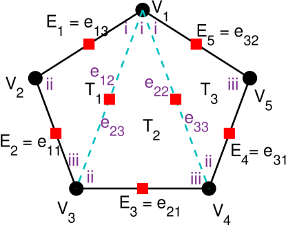
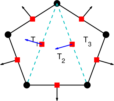
Fig. 1: Illustration of a possible partition of pentagon cell T𝑇T into three subtriangles.

We shall consider a pentagon cell T𝑇T (shown in Figure 1) for deriving the corresponding velocity reconstruction. We first perform the sub-triangulation for this cell T𝑇T into three small triangles Tjsubscript𝑇𝑗T_{j} (j=1,,3𝑗13j=1,\cdots,3). The local indices for sub-triangles are denoted by Roman numbers (i,ii,iii). There are two interior edges in the cell T𝑇T and we shall use the notation eijsubscript𝑒𝑖𝑗e_{ij} to denote the sub-triangle’s indices i𝑖i and j𝑗j. The vertex indices are denoted as Vj (j𝑗j=1,\cdots,5); The boundaries for cell T𝑇T are denoted by Ej (j𝑗j=1,,5151,\cdots,5). All the labels and indexing are demonstrated in Figure 1. For the piecewise polynomial basis, we shall assume the degree of freedom on each sub-triangle is three corresponding to the coefficients to be determined in front of the piecewise RT(Ti)0{}_{0}(T_{i}) (i=1,2,3) basis. Thus in this particular setting, we shall derive a matrix 𝕄𝕄\mathbb{M} with size 9×9999\times 9. By the condition (14a), (14d), and (14e), we assume Πh𝐯=i=13(j=13c3(i1)+jΦj(Ti)(x,y))subscriptΠ𝐯superscriptsubscript𝑖13superscriptsubscript𝑗13subscript𝑐3𝑖1𝑗superscriptsubscriptΦ𝑗subscript𝑇𝑖𝑥𝑦\Pi_{h}{\bf v}=\sum_{i=1}^{3}\left(\sum_{j=1}^{3}c_{3(i-1)+j}\Phi_{j}^{(T_{i})}(x,y)\right), where the basis function Φj(Ti)(x,y)superscriptsubscriptΦ𝑗subscript𝑇𝑖𝑥𝑦\Phi_{j}^{(T_{i})}(x,y) denotes the local RT0 basis with index j𝑗j in the sub-triangle Tisubscript𝑇𝑖T_{i}. On the edge E1subscript𝐸1E_{1}, we only consider the RT0 basis in the subtriangle T1subscript𝑇1T_{1}, and thus (14a) implies

E1Πh𝐯𝐧E1𝑑s=e13j=13cjΦjT1𝐧13ds=e13c3Φ3T1𝐧13𝑑s=c3,subscriptsubscript𝐸1subscriptΠ𝐯subscript𝐧subscript𝐸1differential-d𝑠subscriptsubscript𝑒13superscriptsubscript𝑗13subscript𝑐𝑗subscriptsuperscriptΦsubscript𝑇1𝑗subscript𝐧13𝑑𝑠subscriptsubscript𝑒13subscript𝑐3superscriptsubscriptΦ3subscript𝑇1subscript𝐧13differential-d𝑠subscript𝑐3\displaystyle\int_{E_{1}}\Pi_{h}{\bf v}\cdot{\bf n}_{E_{1}}ds=\int_{e_{13}}\sum_{j=1}^{3}c_{j}\Phi^{T_{1}}_{j}\cdot{\bf n}_{13}ds=\int_{e_{13}}c_{3}\Phi_{3}^{T_{1}}\cdot{\bf n}_{13}ds=c_{3},

which can be written to the first row in the matrix 𝕄𝕄\mathbb{M}. Similarly, one can derive the 2rd to 5th rows for the matrix 𝕄𝕄\mathbb{M}. Then for the condition (14d), we have

00\displaystyle 0 =\displaystyle= e12j=13cjΦj(T1)𝐧e12ds+e23j=13c3+jΦj(T2)𝐧e23dssubscriptsubscript𝑒12superscriptsubscript𝑗13subscript𝑐𝑗superscriptsubscriptΦ𝑗subscript𝑇1subscript𝐧subscript𝑒12𝑑𝑠subscriptsubscript𝑒23superscriptsubscript𝑗13subscript𝑐3𝑗superscriptsubscriptΦ𝑗subscript𝑇2subscript𝐧subscript𝑒23𝑑𝑠\displaystyle\int_{e_{12}}\sum_{j=1}^{3}c_{j}\Phi_{j}^{(T_{1})}\cdot{\bf n}_{e_{12}}ds+\int_{e_{23}}\sum_{j=1}^{3}c_{3+j}\Phi_{j}^{(T_{2})}\cdot{\bf n}_{e_{23}}ds
=\displaystyle= e12(c2Φ2(T1)𝐧e12+c6Φ3(T2)𝐧e23)𝑑s=c2+c6,subscriptsubscript𝑒12subscript𝑐2superscriptsubscriptΦ2subscript𝑇1subscript𝐧subscript𝑒12subscript𝑐6superscriptsubscriptΦ3subscript𝑇2subscript𝐧subscript𝑒23differential-d𝑠subscript𝑐2subscript𝑐6\displaystyle\int_{e_{12}}\left(c_{2}\Phi_{2}^{(T_{1})}\cdot{\bf n}_{e_{12}}+c_{6}\Phi_{3}^{(T_{2})}\cdot{\bf n}_{e_{23}}\right)ds=c_{2}+c_{6},

which gives the 6th row of the matrix 𝕄𝕄\mathbb{M}. Similarly, the 7th row can be obtained in the same way. Next, we shall employ the condition (14e) for deriving the last two rows for the matrix 𝕄𝕄\mathbb{M}. We have

00\displaystyle 0 =\displaystyle= T1(Πh𝐯|T2Πh𝐯|T1)𝑑𝐱=T1(j=13c3+jΦj(T2)j=13cjΦj(T1))𝑑𝐱subscriptsubscript𝑇1evaluated-atsubscriptΠ𝐯subscript𝑇2evaluated-atsubscriptΠ𝐯subscript𝑇1differential-d𝐱subscriptsubscript𝑇1superscriptsubscript𝑗13subscript𝑐3𝑗superscriptsubscriptΦ𝑗subscript𝑇2superscriptsubscript𝑗13subscript𝑐𝑗superscriptsubscriptΦ𝑗subscript𝑇1differential-d𝐱\displaystyle\int_{T_{1}}\nabla\cdot(\Pi_{h}{\bf v}|_{T_{2}}-\Pi_{h}{\bf v}|_{T_{1}})d{\bf x}=\int_{T_{1}}\nabla\cdot\left(\sum_{j=1}^{3}c_{3+j}\Phi_{j}^{(T_{2})}-\sum_{j=1}^{3}c_{j}\Phi_{j}^{(T_{1})}\right)d{\bf x}
=\displaystyle= T1(c422|JT2|+c52|JT2|+c62|JT2|c122|JT1|c22|JT1|c32|JT1|)𝑑𝐱subscriptsubscript𝑇1subscript𝑐422subscript𝐽subscript𝑇2subscript𝑐52subscript𝐽subscript𝑇2subscript𝑐62subscript𝐽subscript𝑇2subscript𝑐122subscript𝐽subscript𝑇1subscript𝑐22subscript𝐽subscript𝑇1subscript𝑐32subscript𝐽subscript𝑇1differential-d𝐱\displaystyle\int_{T_{1}}\left(c_{4}\frac{2\sqrt{2}}{|J_{T_{2}}|}+c_{5}\frac{2}{|J_{T_{2}}|}+c_{6}\frac{2}{|J_{T_{2}}|}-c_{1}\frac{2\sqrt{2}}{|J_{T_{1}}|}-c_{2}\frac{2}{|J_{T_{1}}|}-c_{3}\frac{2}{|J_{T_{1}}|}\right)d{\bf x}
=\displaystyle= |JT1|2(c422|JT2|+c52|JT2|+c62|JT2|c122|JT1|c22|JT1|c32|JT1|)subscript𝐽subscript𝑇12subscript𝑐422subscript𝐽subscript𝑇2subscript𝑐52subscript𝐽subscript𝑇2subscript𝑐62subscript𝐽subscript𝑇2subscript𝑐122subscript𝐽subscript𝑇1subscript𝑐22subscript𝐽subscript𝑇1subscript𝑐32subscript𝐽subscript𝑇1\displaystyle\frac{|J_{T_{1}}|}{2}\left(c_{4}\frac{2\sqrt{2}}{|J_{T_{2}}|}+c_{5}\frac{2}{|J_{T_{2}}|}+c_{6}\frac{2}{|J_{T_{2}}|}-c_{1}\frac{2\sqrt{2}}{|J_{T_{1}}|}-c_{2}\frac{2}{|J_{T_{1}}|}-c_{3}\frac{2}{|J_{T_{1}}|}\right)
=\displaystyle= |T1|(c42|T2|+c51|T2|+c61|T2|c12|T1|c21|T1|c31|T1|)subscript𝑇1subscript𝑐42subscript𝑇2subscript𝑐51subscript𝑇2subscript𝑐61subscript𝑇2subscript𝑐12subscript𝑇1subscript𝑐21subscript𝑇1subscript𝑐31subscript𝑇1\displaystyle|{T_{1}}|\left(c_{4}\frac{\sqrt{2}}{|{T_{2}}|}+c_{5}\frac{1}{|{T_{2}}|}+c_{6}\frac{1}{|{T_{2}}|}-c_{1}\frac{\sqrt{2}}{|{T_{1}}|}-c_{2}\frac{1}{|{T_{1}}|}-c_{3}\frac{1}{|{T_{1}}|}\right)

by using |JTi|=2|Tj|subscript𝐽subscript𝑇𝑖2subscript𝑇𝑗|J_{T_{i}}|=2|T_{j}| and cancelling the common factor gives row 8th. Similarly, the 9th row can be obtained. Thus the matrix can be re-written as follows,

𝕄=[0010000002000000000002000000000002000000000100100010000000100012112|T1||T2||T1||T2||T1||T2|0002110002|T1||T3||T1||T3||T1||T3|].𝕄matrix0010000002000000000002000000000002000000000100100010000000100012112subscript𝑇1subscript𝑇2subscript𝑇1subscript𝑇2subscript𝑇1subscript𝑇20002110002subscript𝑇1subscript𝑇3subscript𝑇1subscript𝑇3subscript𝑇1subscript𝑇3\displaystyle\mathbb{M}=\begin{bmatrix}0&0&1&0&0&0&0&0&0\\ \sqrt{2}&0&0&0&0&0&0&0&0\\ 0&0&0&\sqrt{2}&0&0&0&0&0\\ 0&0&0&0&0&0&\sqrt{2}&0&0\\ 0&0&0&0&0&0&0&1&0\\ 0&1&0&0&0&1&0&0&0\\ 0&0&0&0&1&0&0&0&1\\ -\sqrt{2}&-1&-1&\dfrac{\sqrt{2}|T_{1}|}{|T_{2}|}&\dfrac{|T_{1}|}{|T_{2}|}&\dfrac{|T_{1}|}{|T_{2}|}&0&0&0\\ -\sqrt{2}&-1&-1&0&0&0&\dfrac{\sqrt{2}|T_{1}|}{|T_{3}|}&\dfrac{|T_{1}|}{|T_{3}|}&\dfrac{|T_{1}|}{|T_{3}|}\end{bmatrix}.

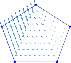
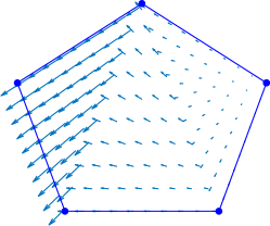
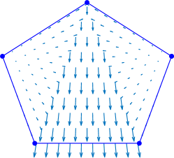
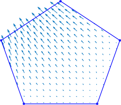
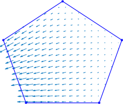
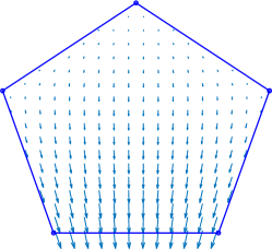
By employing the matrix 𝕄𝕄\mathbb{M} and given 𝐯={𝐯0,𝐯b}𝐯subscript𝐯0subscript𝐯𝑏{\bf v}=\{{\bf v}_{0},{\bf v}_{b}\}, one can construct the linear system 𝕄𝐜=𝐛𝕄𝐜𝐛\mathbb{M}{\bf c}={\bf b} for solving vector coefficients 𝐜=[cj]j=19𝐜superscriptsubscriptdelimited-[]subscript𝑐𝑗𝑗19{\bf c}=[c_{j}]_{j=1}^{9}. For example, assume 𝐯b|E1=𝐧E1evaluated-atsubscript𝐯𝑏subscript𝐸1subscript𝐧subscript𝐸1{\bf v}_{b}|_{E_{1}}={\bf n}_{E_{1}} and 𝐯b|Ej=0evaluated-atsubscript𝐯𝑏subscript𝐸𝑗0{\bf v}_{b}|_{E_{j}}=0 for j=2,,5𝑗25j=2,\dots,5, and then the vector 𝐛𝐛{\bf b} will be calculated by: the first component [𝐛]1=E1𝐯b𝐧E1𝑑s=|E1|subscriptdelimited-[]𝐛1subscriptsubscript𝐸1subscript𝐯𝑏subscript𝐧subscript𝐸1differential-d𝑠subscript𝐸1[{\bf b}]_{1}=\int_{E_{1}}{\bf v}_{b}\cdot{\bf n}_{E_{1}}ds=|E_{1}| and the other components are zeros. The calculated Πh𝐯subscriptΠ𝐯\Pi_{h}{\bf v} corresponding to 𝐯b=𝐧E1subscript𝐯𝑏subscript𝐧subscript𝐸1{\bf v}_{b}={\bf n}_{E_{1}}, 𝐯b=𝐧E2subscript𝐯𝑏subscript𝐧subscript𝐸2{\bf v}_{b}={\bf n}_{E_{2}}, and 𝐯b=𝐧E3subscript𝐯𝑏subscript𝐧subscript𝐸3{\bf v}_{b}={\bf n}_{E_{3}} are plotted in Figure 2. As noted in this plot, on the edge E1subscript𝐸1E_{1}, the projection Πh𝐯subscriptΠ𝐯\Pi_{h}{\bf v} with 𝐯b=𝐧E1subscript𝐯𝑏subscript𝐧subscript𝐸1{\bf v}_{b}={\bf n}_{E_{1}} preserves the quantity E1𝐯b𝐧|E1dsevaluated-atsubscriptsubscript𝐸1subscript𝐯𝑏𝐧subscript𝐸1𝑑𝑠\int_{E_{1}}{\bf v}_{b}\cdot{\bf n}|_{E_{1}}ds.

Refer to caption Refer to caption Refer to caption
(a) (b) (c)
Fig. 2: Illustration of velocity reconstruction Πh𝐯subscriptΠ𝐯\Pi_{h}{\bf v} in the space Λk(T)subscriptΛ𝑘𝑇\Lambda_{k}(T), which is piecewise polynomial: (a) 𝐯b=𝐧E1subscript𝐯𝑏subscript𝐧subscript𝐸1{\bf v}_{b}={\bf n}_{E_{1}}; (b) 𝐯b=𝐧E2subscript𝐯𝑏subscript𝐧subscript𝐸2{\bf v}_{b}={\bf n}_{E_{2}}; (c) 𝐯b=𝐧E3subscript𝐯𝑏subscript𝐧subscript𝐸3{\bf v}_{b}={\bf n}_{E_{3}};
Refer to caption Refer to caption Refer to caption
(a) (b) (c)
Fig. 3: Illustration of velocity reconstruction in the 𝕎0subscript𝕎0\mathbb{CW}_{0} space in the Wachspress Coordinates [22], which consists rational functions: (a) reconstruction of 𝐧E1subscript𝐧subscript𝐸1{\bf n}_{E_{1}}; (b) reconstruction of 𝐧E2subscript𝐧subscript𝐸2{\bf n}_{E_{2}}; (c) reconstruction of 𝐧E3subscript𝐧subscript𝐸3{\bf n}_{E_{3}}.

Next, we compare the bases in Λ0(T)subscriptΛ0𝑇\Lambda_{0}(T) defined above with another polygonal RT0-like bases in the 𝕎0subscript𝕎0\mathbb{CW}_{0} setting on the same pentagon cell, which is generated by employing the Wachspress Coordinates[7]. Three velocity reconstructions based on 𝕎0subscript𝕎0\mathbb{CW}_{0} space, corresponding to 𝐯b=𝐧E1,𝐧E2,𝐧E3subscript𝐯𝑏subscript𝐧subscript𝐸1subscript𝐧subscript𝐸2subscript𝐧subscript𝐸3{\bf v}_{b}={\bf n}_{E_{1}},{\bf n}_{E_{2}},{\bf n}_{E_{3}}, are plotted in Figure 3. As shown in Figure 2-3, the reconstructions in 𝕎0subscript𝕎0\mathbb{CW}_{0} are one piece functions defined on the polygon T𝑇T consisting rational functions; the reconstructions in Λ0(T)subscriptΛ0𝑇\Lambda_{0}(T) are piecewise polynomials with the same normal component crossing the interior edges.

Since the stiffness matrix is the same as that of the previous stabilizer free WG scheme, we shall omit the implementation for the stiffness matrix assembling. In the body source assembling, we shall compute

(𝐟,Πh𝐯)𝐟subscriptΠ𝐯\displaystyle({\bf f},\Pi_{h}{\bf v}) =\displaystyle= T𝒯hi,jc3(i1)+jTi𝐟Φj(Ti)𝑑𝐱=T𝒯h[𝐜][𝐟Φ],subscript𝑇subscript𝒯subscript𝑖𝑗subscript𝑐3𝑖1𝑗subscriptsubscript𝑇𝑖𝐟superscriptsubscriptΦ𝑗subscript𝑇𝑖differential-d𝐱subscript𝑇subscript𝒯superscriptdelimited-[]𝐜topdelimited-[]subscript𝐟Φ\displaystyle\sum_{T\in\mathcal{T}_{h}}\sum_{i,j}c_{3(i-1)+j}\int_{T_{i}}{\bf f}\Phi_{j}^{(T_{i})}d{\bf x}=\sum_{T\in\mathcal{T}_{h}}\left[{\bf c}\right]^{\top}\cdot\left[{\bf f}_{\Phi}\right],

where 𝐟Φsubscript𝐟Φ{\bf f}_{\Phi} denotes the integral of Ti𝐟Φj(Ti)𝑑𝐱subscriptsubscript𝑇𝑖𝐟superscriptsubscriptΦ𝑗subscript𝑇𝑖differential-d𝐱\int_{T_{i}}{\bf f}\Phi_{j}^{(T_{i})}d{\bf x} for each piecewise RT(Ti)0{}_{0}(T_{i}) basis (i=1,,#𝑖1#i=1,\cdots,\#sub-triangles). Different as the basis in the 𝕎0subscript𝕎0\mathbb{CW}_{0} space, which usually contains rational functions, here in our new numerical scheme, the integrand will be a production of 𝐟𝐟{\bf f} and piecewise polynomials. Thus our new constructed projection operator will not introduce extra errors when 𝐟𝐟{\bf f} is non-polynomial function, which is a problem for the 𝕎0subscript𝕎0\mathbb{CW}_{0} space. Besides, the basis functions in 𝕎0subscript𝕎0\mathbb{CW}_{0} are limited to the lowest order and on the convex element. In the sense of generalization to arbitrary scheme order and meshes, our new approach outperforms the scheme by employing 𝕎0subscript𝕎0\mathbb{CW}_{0} spaces[22].

6 Numerical Experiments

This section shows several numerical examples to validate our theoretical conclusions that our proposed approach has one order super-convergence rate than the optimal rate and is also pressure-robust. We shall measure the errors by following norms for the velocity and pressure:

H1-Error |𝐞h|:=|𝐐h𝐮𝐮h|=(T𝒯hT|w(𝐐h𝐮𝐮h)|2𝑑𝐱)1/2,assignsuperscript𝐻1-Error normsubscript𝐞normsubscript𝐐𝐮subscript𝐮superscriptsubscript𝑇subscript𝒯subscript𝑇superscriptsubscript𝑤subscript𝐐𝐮subscript𝐮2differential-d𝐱12\displaystyle H^{1}\text{-Error }{|||}{\bf e}_{h}{|||}:={|||}{\bf Q}_{h}{\bf u}-{\bf u}_{h}{|||}=\left(\sum_{T\in\mathcal{T}_{h}}\int_{T}\left|\nabla_{w}({\bf Q}_{h}{\bf u}-{\bf u}_{h})\right|^{2}d{\bf x}\right)^{1/2},
L2-Error 𝐞0:=𝐐0𝐮𝐮0=(T𝒯hT|𝐐0𝐮𝐮0|2𝑑𝐱)1/2,assignsuperscript𝐿2-Error normsubscript𝐞0normsubscript𝐐0𝐮subscript𝐮0superscriptsubscript𝑇subscript𝒯subscript𝑇superscriptsubscript𝐐0𝐮subscript𝐮02differential-d𝐱12\displaystyle L^{2}\text{-Error }\|{\bf e}_{0}\|:=\|{\bf Q}_{0}{\bf u}-{\bf u}_{0}\|=\left(\sum_{T\in\mathcal{T}_{h}}\int_{T}\left|{\bf Q}_{0}{\bf u}-{\bf u}_{0}\right|^{2}d{\bf x}\right)^{1/2},
L2-Error ϵh:=𝒬hpph:=(T𝒯hT|𝒬hpph|2𝑑𝐱)1/2.assignsuperscript𝐿2-Error normsubscriptitalic-ϵnormsubscript𝒬𝑝subscript𝑝assignsuperscriptsubscript𝑇subscript𝒯subscript𝑇superscriptsubscript𝒬𝑝subscript𝑝2differential-d𝐱12\displaystyle L^{2}\text{-Error }\|\epsilon_{h}\|:=\|\mathcal{Q}_{h}p-p_{h}\|:=\left(\sum_{T\in\mathcal{T}_{h}}\int_{T}\left|\mathcal{Q}_{h}p-p_{h}\right|^{2}d{\bf x}\right)^{1/2}.

As the theoretical conclusions in Theorem 9/11, we expect the errors measured in |𝐞h|normsubscript𝐞{|||}{\bf e}_{h}{|||}, 𝐞0normsubscript𝐞0\|{\bf e}_{0}\|, and ϵhnormsubscriptitalic-ϵ\|\epsilon_{h}\| converge with the orders 𝒪(hk+1)𝒪superscript𝑘1\mathcal{O}(h^{k+1}), 𝒪(hk+2)𝒪superscript𝑘2\mathcal{O}(h^{k+2}), and 𝒪(hk+1)𝒪superscript𝑘1\mathcal{O}(h^{k+1}).

6.1 Simulations with Lowest Degree k=0𝑘0k=0

Let Ω=(0,1)×(0,1)Ω0101\Omega=(0,1)\times(0,1) and the exact solutions are chosen as below for testing:

(70) 𝐮=(10x2y(x1)2(2y1)(y1)10xy2(2x1)(x1)(y1)2),p=10x.formulae-sequence𝐮matrix10superscript𝑥2𝑦superscript𝑥122𝑦1𝑦110𝑥superscript𝑦22𝑥1𝑥1superscript𝑦12𝑝10𝑥\displaystyle{\bf u}=\begin{pmatrix}10x^{2}y(x-1)^{2}(2y-1)(y-1)\\ -10xy^{2}(2x-1)(x-1)(y-1)^{2}\end{pmatrix},\ p=10x.

In the following, we shall test the numerical performance for the lowest order WG element k=0𝑘0k=0.

  • Refer to caption Refer to caption
    (a) (b)
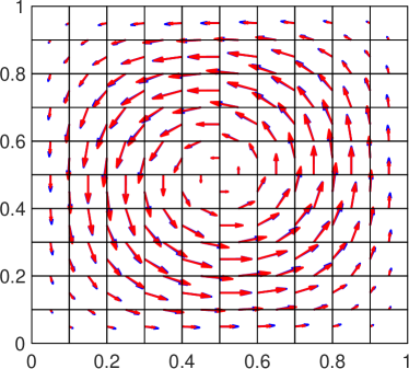
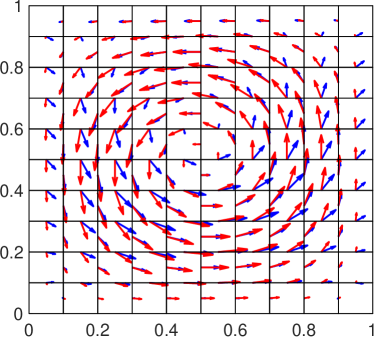
    Fig. 4: Example 6.1. Plot of the vector fields of velocity. Red arrow denotes the exact solution; Blue arrow plots the WG solutions with k=0𝑘0k=0. (a). WG solution by pressure-robust Algorithm 1; (b) WG solution by non-pressure-robust Algorithm 2.
  • Test case with ν=1𝜈1\nu=1 on rectangular grid. In this test, we shall perform WG Algorithm 1 and WG Algorithm 2 and compare the numerical performance on the coarse mesh. Let k=0𝑘0k=0, ν=1𝜈1\nu=1, h=1/10110h=1/10, and the numerical solutions on the uniform rectangular mesh are illustrated in Figure 4. As one can see from these two figures that Algorithm 1 provides a better solution aligning with the exact velocity field. However, the right panel in this figure, produced by Algorithm 2, plots a solution which can not preserve the vector field. It shows that as we modifying the body source assembling but remaining the same stiffness matrix, we are able to improve the simulations in velocity on the uniform rectangular meshes.

    Table 1: Example 6.1. Error profiles and convergence results on the uniform rectangular mesh.
    |𝐞h|normsubscript𝐞{|||}{\bf e}_{h}{|||} rate 𝐞0normsubscript𝐞0\|{\bf e}_{0}\| rate ϵhnormsubscriptitalic-ϵ\|\epsilon_{h}\| rate |𝐞h|normsubscript𝐞{|||}{\bf e}_{h}{|||} rate 𝐞0normsubscript𝐞0\|{\bf e}_{0}\| rate ϵhnormsubscriptitalic-ϵ\|\epsilon_{h}\| rate
    ν𝜈\nu = 1, Pressure Robust Algorithm 1 ν𝜈\nu = 1, Non-Pressure Robust Algorithm 2
    4 2.42E-1 1.02E-2 2.35E-2 8.92E-1 7.34E-2. 7.46E-1
    8 1.36E-1 0.8 3.55E-3 1.5 1.56E-2 0.6 4.88E-1 0.9 2.28E-2 1.7 4.24E-1 0.8
    16 7.04E-2 1.0 1.02E-3 1.8 5.62E-3 1.5 2.52E-1 1.0 6.17E-3 1.9 2.27E-1 0.9
    32 3.55E-2 1.0 2.68E-4 1.9 1.58E-3 1.8 1.28E-1 1.0 1.58E-3 2.0 1.18E-1 0.9
    64 1.78E-2 1.0 6.80E-5 2.0 4.09E-4 2.0 6.40E-2 1.0 3.99E-4 2.0 6.01E-2 1.0
    128 8.91E-3 1.0 1.71E-5 2.0 1.03E-4 2.0 3.20E-2 1.0 9.99E-5 2.0 3.04E-2 1.0
    ν𝜈\nu = 1E-2, Algorithm 1 ν𝜈\nu = 1E-2, Algorithm 2
    4 2.42E-1 1.02E-2 2.35E-4 8.88E+1 7.33. 7.46E-1
    8 1.36E-1 0.8 3.55E-3 1.5 1.56E-4 0.6 4.86E+1 0.9 2.28 1.7 4.24E-1 0.8
    16 7.04E-2 1.0 1.02E-3 1.8 5.62E-5 1.5 2.51E+1 1.0 6.15E-1 1.9 2.27E-1 0.9
    32 3.55E-2 1.0 2.68E-4 1.9 1.58E-5 1.8 1.27E+1 1.0 1.58E-1 2.0 1.18E-1 0.9
    64 1.78E-2 1.0 6.80E-5 2.0 4.09E-6 2.0 6.37 1.0 3.98E-2 2.0 6.01E-2 1.0
    128 8.91E-3 1.0 1.71E-5 2.0 1.03E-6 2.0 3.19 1.0 9.97E-3 2.0 3.04E-2 1.0
    ν𝜈\nu = 1E-4, Algorithm 1 ν𝜈\nu = 1E-4, Algorithm 2
    4 2.42E-1 1.02E-2 2.35E-6 8.88E+3 7.33E+2 7.46E-1
    8 1.36E-1 0.8 3.55E-3 1.5 1.56E-6 0.6 4.86E+3 0.9 2.28E+2 1.7 4.24E-1 0.8
    16 7.04E-2 1.0 1.02E-3 1.8 5.62E-7 1.5 2.51E+3 1.0 6.15E+1 1.9 2.27E-1 0.9
    32 3.55E-2 1.0 2.68E-4 1.9 1.58E-7 1.8 1.27E+3 1.0 1.58E+1 2.0 1.18E-1 0.9
    64 1.78E-2 1.0 6.80E-5 2.0 4.09E-8 2.0 6.37E+2 1.0 3.98 2.0 6.01E-2 1.0
    128 8.91E-3 1.0 1.71E-5 2.0 1.03E-8 2.0 3.19E+2 1.0 9.97E-1 2.0 3.04E-2 1.0
  • Test with various values in ν𝜈\nu. In this test, we choose ν=1,𝜈1\nu=1, 1E-2, and 1E-4 to validate the robustness for the proposed numerical scheme. Table 1 reports the error profiles and convergence results. The performance can be summarized as below.

    • The convergence orders for velocity obtained from Algorithm 1 and Algorithm 2 agree with our theoretical conclusions. We have the errors measured in |𝐞h|normsubscript𝐞{|||}{\bf e}_{h}{|||}, 𝐞0normsubscript𝐞0\|{\bf e}_{0}\| converging at the orders 𝒪(h)𝒪\mathcal{O}(h), 𝒪(h2)𝒪superscript2\mathcal{O}(h^{2}), and 𝒪(h)𝒪\mathcal{O}(h) respectively.

    • As we reduce the values in ν𝜈\nu, Algorithm 1 preserve the accuracy in velocity. However, the velocity error delivered by Algorithm 2 is increasing by a factor 1/ν1𝜈1/\nu, though the convergence rate is still preserved.

    • In the pressure simulation, the numerical solution produced by Algorithm 2 preserve the same accuracy for various viscosity and converges at the order 𝒪(h)𝒪\mathcal{O}(h). In the opposite, Algorithm 1 produces the numerical pressure with super-convergence rate 𝒪(h2)𝒪superscript2\mathcal{O}(h^{2}). Besides, as we reduce the values in ν𝜈\nu, the error in pressure is also reduced by ν𝜈\nu.

    • Thus, the new pressure-robust scheme provides a significant better simulation for small viscosity compared to the previous scheme Algorithm 2.
    Refer to caption Refer to caption Refer to caption Refer to caption
    (a) (b) (c) (d)
    Refer to caption Refer to caption Refer to caption Refer to caption
    (e) (f) (g) (h)
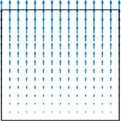
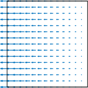
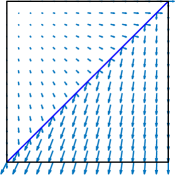
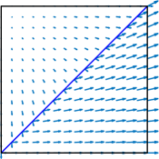
    Fig. 5: Example 6.1. Illustration of the bases for RT[0](T) and Λ0(T)subscriptΛ0𝑇\Lambda_{0}(T).
    Refer to caption
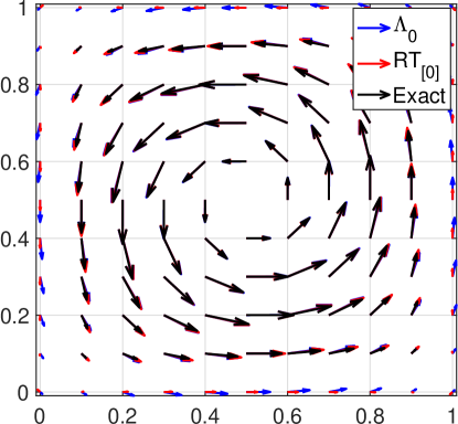
    Fig. 6: Example 6.1. Vector plots for employing Λ0subscriptΛ0\Lambda_{0}, RT[0] spaces in the velocity reconstruction and exact solution on the mesh with h=1/10110h=1/10 and ν=1010𝜈superscript1010\nu=10^{-10}.
    Table 2: Example 6.1. Error profiles for Λ0subscriptΛ0\Lambda_{0} and RT[0] elements for various values in ν𝜈\nu.
    Λ0subscriptΛ0\Lambda_{0} RT[0](T)subscriptRTdelimited-[]0𝑇\text{RT}_{[0]}(T)
    |𝐞h|normsubscript𝐞{|||}{\bf e}_{h}{|||} 𝐞0normsubscript𝐞0\|{\bf e}_{0}\| ϵhnormsubscriptitalic-ϵ\|\epsilon_{h}\| |𝐞h|normsubscript𝐞{|||}{\bf e}_{h}{|||} 𝐞0normsubscript𝐞0\|{\bf e}_{0}\| ϵhnormsubscriptitalic-ϵ\|\epsilon_{h}\|
    ν=1𝜈1\nu=1 2.8461E-2 1.7287E-4 1.0284E-3 4.3881E-2 4.5269E-4 6.7309E-3
    ν=1𝜈1\nu=1E-2 2.8461E-2 1.7287E-4 1.0284E-5 4.3881E-2 4.5269E-4 6.7309E-5
    ν=1𝜈1\nu=1E-4 2.8461E-2 1.7287E-4 1.0284E-7 4.3881E-2 4.5269E-4 6.7309E-7
    ν=1𝜈1\nu=1E-6 2.8461E-2 1.7287E-4 1.0284E-9 4.3881E-2 4.5269E-4 6.7309E-9
    ν=1𝜈1\nu=1E-8 2.8461E-2 1.7287E-4 1.0283E-11 4.3881E-2 4.5269E-4 6.7310E-11
    ν=1𝜈1\nu=1E-10 2.8461E-2 1.7287E-4 1.0284E-13 4.3881E-2 4.5265E-4 7.6583E-13
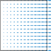
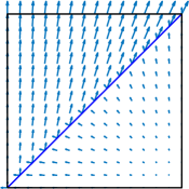
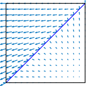
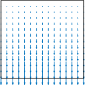
  • Comparison with RT(T)[0]{}_{[0]}(T) space on the rectangular mesh. In this test, we compare the numerical performance of employing the rectangular RT element[1] with k=0𝑘0k=0 (denoted as RT[0]) and our proposed projection space Λ0(T)subscriptΛ0𝑇\Lambda_{0}(T). We compute the velocity reconstructions Πh𝐯subscriptΠ𝐯\Pi_{h}{\bf v}, respectively, into the spaces RT(T)[0]{}_{[0]}(T) and Λ0(T)subscriptΛ0𝑇\Lambda_{0}(T). Four basis functions on unit square are plotted in Figure 5. It is noted that the constructed basis in the Λ0(T)subscriptΛ0𝑇\Lambda_{0}(T) space is piecewise polynomial with normal component continuous cross the interior edge. We plot the numerical vector field in Figure 6 on the mesh with h=1/10110h=1/10 and ν=1010𝜈superscript1010\nu=10^{-10} for the Λ0subscriptΛ0\Lambda_{0} and RT[0] version. The numerical vector fields generated by employing Λ0subscriptΛ0\Lambda_{0} and RT[0] spaces agree well with the exact vector field. This observation validates that both of the tests are pressure robust. Furthermore, the error profiles for various values in ν𝜈\nu are reported in Table 2. It can be validated again from this table that by employing the velocity reconstruction both into Λ0subscriptΛ0\Lambda_{0} and RT[0] spaces will produce the pressure robust simulation. Also the errors in the Λ0subscriptΛ0\Lambda_{0} version are slightly better than that of the RT[0] space.

    Refer to caption Refer to caption
    (a) (b)
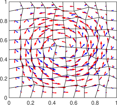
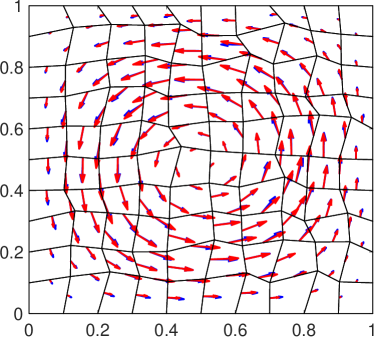
    Fig. 7: Example 6.1. Plot of the velocity vector fields. Red arrow denotes the exact solution; Blue arrow plots the numerical solution. (a) Algorithm 2; (b) Algorithm 1.
  • Test case with ν=1𝜈1\nu=1 on deformed rectangular grid. In this test, we shall perform WG Algorithm 1-2 on the deformed rectangular grid and compare the numerical performance on the coarse mesh. Let k=0𝑘0k=0 and h=1/10110h=1/10 and the numerical solutions on the uniform rectangular mesh are plotted in Figure 7. The pressure robust scheme improves the velocity simulation and preserves very well the exact velocity vector field.

6.2 Effects from the Approximation with Pressure

Let Ω=(0,1)2Ωsuperscript012\Omega=(0,1)^{2} and the external body force 𝐟𝐟{\bf f} be chosen such that the exact solutions are

(71) 𝐮=0, and p(x,y)=j=07xjy7j7611260.formulae-sequence𝐮0 and 𝑝𝑥𝑦superscriptsubscript𝑗07superscript𝑥𝑗superscript𝑦7𝑗7611260\displaystyle{\bf u}=0,\text{ and }p(x,y)=\sum_{j=0}^{7}x^{j}y^{7-j}-\frac{761}{1260}.

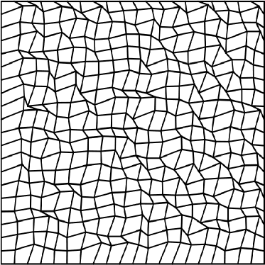
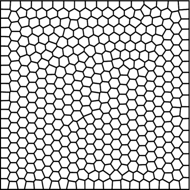
In this test, we perform WG Algorithm 1 on the deformed rectangular mesh and the polygonal mesh shown in Figure 8. We shall employ the velocity reconstruction operator into the Λ0subscriptΛ0\Lambda_{0} and 𝕎0subscript𝕎0\mathbb{CW}_{0} spaces and check the corresponding robustness. The scheme with respect to 𝕎0subscript𝕎0\mathbb{CW}_{0} space was investigated in [22].

Refer to caption Refer to caption
(a) (b)
Fig. 8: Example 6.2.1. illustration of the polygonal grids. (a) Deformed rectangular grid; (b) Polygonal grid.

6.2.1 Test - deformed rectangular mesh

In this section, we perform the weak Galerkin Algorithm on the deformed rectangular mesh (Figure 8a). Since this mesh contains non-convex cell, the 𝕎0subscript𝕎0\mathbb{CW}_{0} basis can not be applied as the velocity reconstruction space. However, our proposed Λ0subscriptΛ0\Lambda_{0} space can be directly chosen for the velocity reconstruction.

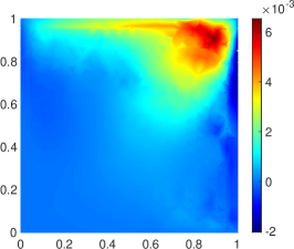
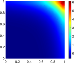
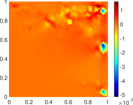
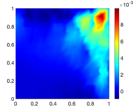
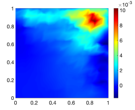
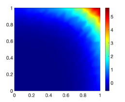
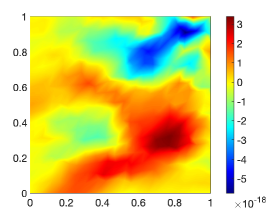
The numerical results corresponding to Algorithm 2 and Algorithm 1 are plotted in Figure 9-10. We observe that:

  • The non-pressure robust scheme produces a numerical velocity with magnitude at the order 𝒪(103)𝒪superscript103\mathcal{O}(10^{-3}). Thus, the error in pressure, in fact, gives rise to the inaccuracy in the velocity simulation. This visualizes the lack of pressure-robustness.

  • By only modifying the body source assembling, we can obtain the pressure robust results. The numerical solutions corresponding to Algorithm 1 are plotted in Figure 10. It is noted that the velocity simulation is almost zero and very closed to the expected zero flow, which is at the order 𝒪(1018)𝒪superscript1018\mathcal{O}(10^{-18}).

  • The above observations validate our enhanced discretization on the non-convex meshes.

Refer to caption Refer to caption Refer to caption
(a) (b) (c)
Fig. 9: Test 6.2.1. Illustration of numerical solutions from Algorithm 2 on the deformed rectangular grid. (a). x-component of velocity; (b) y-component of velocity; (c) pressure.
Refer to caption Refer to caption Refer to caption
(a) (b) (c)
Fig. 10: Test 6.2.1. Illustration of numerical solutions from Algorithm 1 on the deformed rectangular grid. (a). x-component of velocity; (b) y-component of velocity; (c) pressure.

6.2.2 Test - polygonal mesh

In this test, we shall perform the simulations on the polygonal grid and compare the numerical performance with the scheme in 𝕎0subscript𝕎0\mathbb{CW}_{0} setting[22]. It is noted that 𝕎0subscript𝕎0\mathbb{CW}_{0} basis on the polygonal mesh usually consists of rational functions and thus in some cases the numerical integration cannot calculated exactly. Such inaccuracy in numerical integration will introduce errors in velocity simulation even though the scheme is designed with pressure-robust property. This test will show that be employing the Λ0subscriptΛ0\Lambda_{0} space we proposed in this paper, we can overcome such inaccuracy integral and achieve complete independency in the velocity simulation.
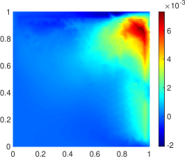
Refer to caption Refer to caption Refer to caption
(a) (b) (c)
Fig. 11: Test 6.2.2. Illustration of numerical solutions from Algorithm 2 on the polygonal grid. (a). x-component of velocity; (b) y-component of velocity; (c) pressure.
Refer to caption Refer to caption Refer to caption
(a) (b) (c)
Fig. 12: Test 6.2.2. Illustration of numerical solutions from Algorithm on the polygonal grid with 𝕎0subscript𝕎0\mathbb{CW}_{0}[22]. (a). x-component of velocity; (b) y-component of velocity; (c) pressure.
Refer to caption Refer to caption Refer to caption
(a) (b) (c)
Fig. 13: Test 6.2.2. Illustration of numerical solutions from Algorithm 1 on the polygonal grid with Λ0subscriptΛ0\Lambda_{0}. (a). x-component of velocity; (b) y-component of velocity; (c) pressure.

We perform the simulations by the non-pressure robust and pressure robust Algorithms and the numerical solutions are plotted in Figure 11-13. When the non-pressure robust has been employed, both reconstruction spaces in 𝕎0subscript𝕎0\mathbb{CW}_{0} and Λ0subscriptΛ0\Lambda_{0} version will deliver poor numerical velocity. The velocity plots from Λ0subscriptΛ0\Lambda_{0} setting are shown in Figure 11a-b and the velocity from 𝕎0subscript𝕎0\mathbb{CW}_{0} is very similar and we omit the plotting here. Now we modify the body force simulation by employing the velocity reconstruction in the 𝕎0subscript𝕎0\mathbb{CW}_{0} and Λ0subscriptΛ0\Lambda_{0} spaces to retrieve the pressure robustness. Due to the invariant of pressure, we expect the numerical velocity is close to zero. The results by employing 𝕎0subscript𝕎0\mathbb{CW}_{0} space are plotted in Figure 12. As one can observe that on the same level of the mesh, the magnitude of velocity is reduce from the order 𝒪(103)𝒪superscript103\mathcal{O}(10^{-3}) to 𝒪(107)𝒪superscript107\mathcal{O}(10^{-7}). The difference from zero flow is due to the inaccuracy for the involving rational functions in the integration for the 𝕎0subscript𝕎0\mathbb{CW}_{0} space. In contrast, as employing the velocity reconstruction operator in the proposed Λ0subscriptΛ0\Lambda_{0} space consisting piecewise polynomials, we overcome the limitation generated by rational functions and retrieve enhanced velocity simulation with the magnitude at the order 𝒪(1018)𝒪superscript1018\mathcal{O}(10^{-18}). This example justified one advantage by our scheme than the work in [22].

6.3 Simulations with Higher Order WG Element

In this section, we shall perform the WG algorithm with high order WG elements and validate our theoretical conclusions.

6.3.1 Convergence test - smooth solutions

Let Ω=(0,1)2Ωsuperscript012\Omega=(0,1)^{2} and we choose the following analytical solutions for the convergence test:

𝐮=(sin(πx)sin(πy)cos(πx)cos(πy)),p(x,y)=2cos(πx)sin(πy).formulae-sequence𝐮matrix𝜋𝑥𝜋𝑦𝜋𝑥𝜋𝑦𝑝𝑥𝑦2𝜋𝑥𝜋𝑦\displaystyle{\bf u}=\begin{pmatrix}\sin(\pi x)\sin(\pi y)\\ \cos(\pi x)\cos(\pi y)\end{pmatrix},\ p(x,y)=2\cos(\pi x)\sin(\pi y).

The performance on a sequence of deformed rectangular mesh (similar as Figure 8a) is summarized as below.

  • Table 3: Example 6.3.1. Error profiles and convergence results for ν=1𝜈1\nu=1 on deformed rectangular mesh.
    Non-Pressure Robust Algorithm 2 Pressure Robust Algorithm 1
    1/h11/h |𝐞h|normsubscript𝐞{|||}{\bf e}_{h}{|||} rate 𝐞0normsubscript𝐞0\|{\bf e}_{0}\| rate ϵhnormsubscriptitalic-ϵ\|\epsilon_{h}\| rate |𝐞h|normsubscript𝐞{|||}{\bf e}_{h}{|||} rate 𝐞0normsubscript𝐞0\|{\bf e}_{0}\| rate ϵhnormsubscriptitalic-ϵ\|\epsilon_{h}\| rate
    k𝑘k = 0
    4 5.01E-1 3.16E-2 3.11E-1 1.01 7.00E-2 1.15
    8 2.72E-1 0.9 1.03E-2 1.6 2.64E-1 0.2 5.84E-1 0.8 2.36E-2 1.6 8.21E-1 0.5
    16 1.41E-1 0.9 2.97E-3 1.8 1.60E-1 0.7 3.10E-1 0.9 7.02E-3 1.7 4.87E-1 0.8
    32 7.16E-2 1.0 7.86E-4 1.9 8.53E-2 0.9 1.59E-1 1.0 1.88E-3 1.9 2.62E-1 0.9
    64 3.60E-2 1.0 2.00E-4 2.0 4.37E-2 1.0 8.00E-2 1.0 4.82E-4 2.0 1.36E-1 1.0
    k𝑘k = 1
    4 8.02E-2 2.19E-3 5.79E-2 2.15E-1 6.61E-3 7.80E-2
    8 2.31E-2 1.8 2.70E-4 3.0 9.57E-3 2.6 5.84E-2 1.9 8.71E-4 2.9 1.06E-2 2.9
    16 6.12E-3 1.9 3.35E-5 3.0 1.40E-3 2.8 1.50E-2 2.0 1.11E-4 3.0 1.35E-3 3.0
    32 1.57E-3 2.0 4.20E-6 3.0 2.07E-4 2.8 3.77E-3 2.0 1.40E-5 3.0 1.70E-4 3.0
    64 3.97E-4 2.0 5.29E-7 3.0 3.19E-5 2.7 9.45E-4 2.0 1.75E-6 3.0 2.14E-5 3.0
    k𝑘k = 2
    4 9.03E-3 1.79E-4 4.01E-3 2.57E-2   5.10E-4 5.84E-3
    8 1.22E-3 2.9 1.05E-5 4.1 5.56E-4 2.8 3.34E-3 2.9 3.23E-5 4.0 5.56E-4 3.4
    16 1.58E-4 2.9 6.44E-7 4.0 7.02E-5 3.0 4.23E-4 3.0 2.04E-6 4.0 6.84E-5 3.0
    32 2.01E-5 3.0 4.00E-8 4.0 8.71E-6 3.0 5.32E-5 3.0 1.28E-7 4.0 8.52E-6 3.0
    64 2.54E-6 3.0 2.50E-9 4.0 1.08E-6 3.0 6.66E-6 3.0 8.00E-9 4.0 1.06E-6 3.0
    k𝑘k = 3
    4 7.96E-4 1.42E-5 2.54E-4 2.42E-3 4.23E-5 6.47E-4
    8 5.32E-5 3.9 4.86E-7 4.9 1.28E-5 4.3 1.59E-4 3.9 1.42E-6 4.9 3.11E-5 4.4
    16 3.43E-6 4.0 1.58E-8 4.9 6.69E-7 4.3 1.01E-5 4.0 4.52E-8 5.0 1.59E-6 4.3
    32 2.18E-7 4.0 5.01E-10 5.0 3.74E-8 4.2 6.36E-7 4.0 1.42E-9 5.0 8.83E-8 4.2
    64 1.37E-8 4.0 1.58E-11 5.0 2.20E-9 4.1 3.99E-8 4.0 4.45E-11 5.0 5.17E-9 4.1
    k𝑘k = 4
    4 5.84E-5 9.04E-7 1.27E-5 1.86E-4 2.67E-6 3.57E-5
    8 1.88E-6 5.0 1.44E-8 6.0 4.48E-7 4.8 5.91E-6 5.0 4.27E-8 6.0 9.45E-7 5.2
    16 5.95E-8 5.0 2.27E-10 6.0 1.42E-8 5.0 1.86E-7 5.0 6.72E-10 6.0 2.79E-8 5.1
    32 1.87E-9 5.0 3.56E-12 6.0 4.36E-10 5.0 5.83E-9 5.0 1.05E-11 6.0 8.40E-10 5.1
  • Test case with ν=1𝜈1\nu=1 on the deformed rectangular meshes. First the non-pressure robust Algorithm 2 and pressure robust Algorithm 1 have been carried out for various WG elements with k=0,1,2,3,4𝑘01234k=0,1,2,3,4. Table 3 reports the error profiles and convergence results. It can be seen from this table that the velocity errors measured in ||||||{|||}\cdot{|||}-norm and L2superscript𝐿2L^{2}-norm converge at the orders 𝒪(hk+1)𝒪superscript𝑘1\mathcal{O}(h^{k+1}) and 𝒪(hk+2)𝒪superscript𝑘2\mathcal{O}(h^{k+2}), which is one order higher than the optimal rate in convergence. The pressure error measured in L2superscript𝐿2L^{2}-norm converges at least 𝒪(hk+1)𝒪superscript𝑘1\mathcal{O}(h^{k+1}). The errors from these two algorithms are the same magnitude.

    Table 4: Example 6.1. Error profiles and convergence results for ν=1𝜈1\nu=1E-2 on deformed rectangular mesh.
    Non-Pressure Robust Algorithm 2 Pressure Robust Algorithm 1
    1/h11/h |𝐞h|normsubscript𝐞{|||}{\bf e}_{h}{|||} rate 𝐞0normsubscript𝐞0\|{\bf e}_{0}\| rate ϵhnormsubscriptitalic-ϵ\|\epsilon_{h}\| rate |𝐞h|normsubscript𝐞{|||}{\bf e}_{h}{|||} rate 𝐞0normsubscript𝐞0\|{\bf e}_{0}\| rate ϵhnormsubscriptitalic-ϵ\|\epsilon_{h}\| rate
    k𝑘k = 0
    4 3.46E+1 3.01 1.84E-1 1.01 7.00E-2 1.15E-2
    8 2.06E+1 0.7 1.03 1.6 1.58E-1 0.2 5.84E-1 0.8 2.36E-2 1.6 8.21E-3 0.5
    16 1.10E+1 0.9 2.91E-1 1.8 1.26E-1 0.3 3.10E-1 0.9 7.02E-3 1.7 4.87E-3 0.8
    32 5.61 1.0 7.65E-2 1.9 7.61E-2 0.7 1.59E-1 1.0 1.88E-3 1.9 2.62E-3 0.9
    64 2.83 1.0 1.94E-2 2.0 4.14E-2 0.9 8.00E-2 1.0 4.82E-4 2.0 1.36E-3 1.0
    k𝑘k = 1
    4 7.39 2.05E-1 4.12E-2 2.15E-1 6.61E-3 7.80E-4
    8 2.12 1.8 2.47E-2 3.1 7.51E-3 2.5 5.84E-2 1.9 8.71E-4 2.9 1.06E-4 2.9
    16 5.57E-1 1.9 3.01E-3 3.0 1.15E-3 2.7 1.50E-2 2.0 1.11E-4 3.0 1.35E-5 3.0
    32 1.42E-1 2.0 3.76E-4 3.0 1.69E-4 2.8 3.77E-3 2.0 1.40E-5 3.0 1.70E-6 3.0
    64 3.59E-2 2.0 4.72E-5 3.0 2.55E-5 2.7 9.45E-4 2.0 1.75E-6 3.0 2.14E-7 3.0
    k𝑘k = 2
    4 8.58E-1 1.61E-2 2.68E-3 2.57E-2 5.10E-4 5.84E-5
    8 1.14E-1 2.9 9.47E-4 4.1 4.48E-4 2.6 3.34E-3 2.9 3.23E-5 4.0 5.56E-6 3.4
    16 1.46E-2 3.0 5.76E-5 4.0 6.00E-5 2.9 4.23E-4 3.0 2.04E-6 4.0 6.84E-7 3.0
    32 1.85E-3 3.0 3.57E-6 4.0 7.58E-6 3.0 5.32E-5 3.0 1.28E-7 4.0 8.52E-8 3.0
    64 2.33E-4 3.0 2.22E-7 4.0 9.47E-7 3.0 6.66E-6 3.0 8.00E-9 4.0 1.06E-8 3.0
    k𝑘k = 3
    4 7.64E-2 1.37E-3 2.46E-4 2.42E-3 4.23E-5 6.47E-6
    8 5.12E-3 3.9 4.70E-5 4.9 1.20E-5 4.4 1.59E-4 3.9 1.42E-6 4.9 3.11E-7 4.4
    16 3.29E-4 4.0 1.52E-6 4.9 6.29E-7 4.2 1.01E-5 4.0 4.52E-8 5.0 1.59E-8 4.3
    32 2.08E-5 4.0 4.83E-8 5.0 3.59E-8 4.1 6.36E-7 4.0 1.42E-9 5.0 8.83E-10 4.2
    64 1.31E-6 4.0 1.52E-9 5.0 2.14E-9 4.1 3.99E-8 4.0 4.45E-11 5.0 5.17E-11 4.1
    k𝑘k = 4
    4 5.65E-3 8.69E-5 1.27E-5 1.86E-4 2.67E-6 3.57E-7
    8 1.83E-4 4.9 1.40E-6 6.0 4.13E-7 4.9 5.91E-6 5.0 4.27E-8 6.0 9.45E-9 5.2
    16 5.79E-6 5.0 2.21E-8 6.0 1.30E-8 5.0 1.86E-7 5.0 6.72E-10 6.0 2.79E-10 5.1
    32 1.82E-7 5.0 3.47E-10 6.0 3.99E-10 5.0 5.83E-9 5.0 1.05E-11 6.0 8.47E-12 5.0
  • Test case with ν𝜈\nu=1E-2 and 1E-4 on the deformed rectangular meshes. The numerical performance corresponding to small values in ν𝜈\nu is reported in Table 4-5. As one reduces the value in ν𝜈\nu, the velocity error produced by non-pressure robust scheme is increasing by a factor 1/ν1𝜈1/\nu, though preserves the expected convergence rate. In contrast, the velocity error produced by the pressure robust scheme preserve the accuracy and convergence order. Thus our proposed Algorithm 1 shows the significant enhancement in velocity simulation. For the pressure simulation, we observe opposite results. As we decreasing the values in ν𝜈\nu, the pressure errors produced by Algorithm 2 remain the same magnitude. However, the pressure errors generated by pressure-robust scheme Algorithm 1 is also reduced by a factor ν𝜈\nu.

    Table 5: Example 6.1. Error profiles and convergence results for ν=1𝜈1\nu=1E-4 on deformed rectangular mesh.
    Non-Pressure Robust Algorithm 2 Pressure Robust Algorithm 1
    1/h11/h |𝐞h|normsubscript𝐞{|||}{\bf e}_{h}{|||} rate 𝐞0normsubscript𝐞0\|{\bf e}_{0}\| rate ϵhnormsubscriptitalic-ϵ\|\epsilon_{h}\| rate |𝐞h|normsubscript𝐞{|||}{\bf e}_{h}{|||} rate 𝐞0normsubscript𝐞0\|{\bf e}_{0}\| rate ϵhnormsubscriptitalic-ϵ\|\epsilon_{h}\| rate
    k𝑘k = 0
    4 3.46E+3 3.01E+2 1.86E-1 1.01 7.00E-2 1.15E-4
    8 2.06E+3 0.7 1.03E+2 1.6 1.57E-1 0.2 5.84E-1 0.8 2.36E-2 1.6 8.21E-5 0.5
    16 1.10E+3 0.9 2.91E+1 1.8 1.26E-1 0.3 3.10E-1 0.9 7.02E-3 1.7 4.87E-5 0.8
    32 5.61E+2 1.0 7.65 1.9 7.60E-2 0.7 1.59E-1 1.0 1.88E-3 1.9 2.62E-5 0.9
    64 2.83E+2 1.0 1.94 2.0 4.13E-2 0.9 8.00E-2 1.0 4.82E-4 2.0 1.36E-5 1.0
    k𝑘k = 1
    4 7.40E+2 2.05E+1 4.10E-2 2.15E-1 6.61E-3 7.80E-6
    8 2.12E+2 1.8 2.47 3.1 7.49E-3 2.5 5.84E-2 1.9 8.71E-4 2.9 1.06E-6 2.9
    16 5.57E+1 1.9 3.01E-1 3.0 1.15E-3 2.7 1.50E-2 2.0 1.11E-4 3.0 1.35E-7 3.0
    32 1.42E+1 2.0 3.76E-2 3.0 1.69E-4 2.8 3.77E-3 2.0 1.40E-5 3.0 1.70E-8 3.0
    64 3.59E 2.0 4.72E-3 3.0 2.55E-5 2.7 9.45E-4 2.0 1.75E-6 3.0 2.14E-9 3.0
    k𝑘k = 2
    4 8.58E+1 1.61 2.67E-3 2.57E-2 5.10E-4 5.84E-7
    8 1.14E+1 2.9 9.46E-2 4.1 4.47E-4 2.6 3.34E-3 2.9 3.23E-5 4.0 5.56E-8 3.4
    16 1.46E 3.0 5.76E-3 4.0 5.99E-5 2.9 4.23E-4 3.0 2.04E-6 4.0 6.84E-9 3.0
    32 1.85E-1 3.0 3.57E-4 4.0 7.57E-6 3.0 5.32E-5 3.0 1.28E-7 4.0 8.52E-10 3.0
    64 2.33E-2 3.0 2.22E-5 4.0 9.45E-7 3.0 6.66E-6 3.0 8.00E-9 4.0 1.06E-10 3.0
    k𝑘k = 3
    4 7.64E 1.37E-1 2.46E-4 2.42E-3 4.23E-5 6.47E-8
    8 5.12E-1 3.9 4.70E-3 4.9 1.20E-5 4.4 1.59E-4 3.9 1.42E-6 4.9 3.11E-9 4.4
    16 3.29E-2 4.0 1.52E-4 4.9 6.29E-7 4.2 1.01E-5 4.0 4.52E-8 5.0 1.59E-10 4.3
    32 2.08E-3 4.0 4.83E-6 5.0 3.59E-8 4.1 6.36E-7 4.0 1.42E-9 5.0 8.84E-12 4.2
    64 1.31E-4 4.0 1.52E-7 5.0 2.14E-9 4.1 3.99E-8 4.0 4.45E-11 5.0 5.18E-13 4.1
    k𝑘k = 4
    4 5.65E-1 8.69E-3 1.27E-5 1.86E-4 2.67E-6 3.57E-9
    8 1.83E-2 4.9 1.40E-4 6.0 4.13E-7 4.9 5.91E-6 5.0 4.27E-8 6.0 9.45E-11 5.2
    16 5.79E-4 5.0 2.21E-6 6.0 1.29E-8 5.0 1.86E-7 5.0 6.72E-10 6.0 2.82E-12 5.1
    32 1.82E-5 5.0 3.47E-8 6.0 3.98E-10 5.0 5.83E-9 5.0 1.55E-11 5.4 1.14E-13 4.6

Next, two algorithms are performed on a sequence of polygonal mesh (Mesh Level 3 is shown in Figure 8b). Similar numerical conclusions as follows can be obtained.

  • Test case with ν=1𝜈1\nu=1 on polygonal mesh. All errors generated by Algorithm 1 and Algorithm 2 converge at the expected order. Though some inconsistency error involved in Algorithm 1, the numerical errors are at comparable magnitude. This observation validate the accuracy of our proposed scheme.

    Table 6: Example 6.1. Error profiles and convergence results for ν=1𝜈1\nu=1 on the polygonal grids.
    Non-Pressure Robust Algorithm 2 Pressure Robust Algorithm 1
    Mesh |𝐞h|normsubscript𝐞{|||}{\bf e}_{h}{|||} rate 𝐞0normsubscript𝐞0\|{\bf e}_{0}\| rate ϵhnormsubscriptitalic-ϵ\|\epsilon_{h}\| rate |𝐞h|normsubscript𝐞{|||}{\bf e}_{h}{|||} rate 𝐞0normsubscript𝐞0\|{\bf e}_{0}\| rate ϵhnormsubscriptitalic-ϵ\|\epsilon_{h}\| rate
    k𝑘k = 0
    Level 1 6.92E-1 5.22E-2 1.55E-1 1.27 9.21E-2 1.29
    Level 2 3.61E-1 0.9 1.38E-2 1.9 1.37E-1 0.2 7.93E-1 0.7 2.98E-2 1.6 4.18E-1 1.6
    Level 3 1.76E-1 1.0 3.60E-3 1.9 6.40E-2 1.1 4.18E-1 0.9 9.12E-3 1.7 1.41E-1 1.6
    Level 4 8.67E-2 1.0 8.66E-4 2.1 2.16E-2 1.6 2.17E-1 0.9 2.48E-3 1.9 8.01E-2 0.8
    Level 5 4.33E-2 1.0 2.17E-4 2.0 7.64E-3 1.5 1.10E-1 1.0 6.40E-4 2.0 1.39E-2 2.5
    k𝑘k = 1
    Level 1 6.21E-2 1.89E-3 4.10E-2 1.85E-1 5.86E-3 6.04E-2
    Level 2 1.59E-2 2.0 2.28E-4 3.0 2.88E-3 3.8 5.41E-2 1.8 5.41E-4 3.4 1.09E-2 2.5
    Level 3 3.92E-3 2.0 2.53E-5 3.2 3.44E-4 3.1 1.34E-2 2.0 7.03E-5 2.9 2.38E-3 2.2
    Level 4 1.02E-3 1.9 3.11E-6 3.0 8.80E-5 2.0 3.44E-3 2.0 8.88E-6 3.0 8.50E-4 1.5
    Level 5 2.49E-4 2.0 3.90E-7 3.0 2.03E-5 2.1 8.68E-4 2.0 1.10E-6 3.0 1.45E-4 2.6
    k𝑘k = 2
    Level 1 8.11E-3 1.52E-4 4.18E-3 2.18E-2 4.86E-4 5.96E-3
    Level 2 8.57E-4 3.2 9.25E-6 4.0 3.40E-4 3.6 2.89E-3 2.9 2.53E-5 4.3 6.76E-4 3.1
    Level 3 1.06E-4 3.0 5.40E-7 4.1 2.24E-5 3.9 3.60E-4 3.0 1.74E-6 3.9 8.23E-5 3.0
    Level 4 1.28E-5 3.1 3.37E-8 4.0 3.73E-6 2.6 4.61E-5 3.0 1.16E-7 3.9 1.23E-5 2.7
    Level 5 1.57E-6 3.0 2.09E-9 4.0 2.27E-7 4.0 5.90E-6 3.0 7.49E-9 4.0 1.25E-6 3.3
    k𝑘k = 3
    Level 1 6.31E-4 1.12E-5 1.81E-4 1.85E-3 3.30E-5 5.73E-4
    Level 2 3.29E-5 4.3 2.95E-7 5.2 1.05E-5 4.1 1.27E-4 3.9 9.89E-7 5.1 3.03E-5 4.2
    Level 3 1.98E-6 4.1 8.50E-9 5.1 5.65E-7 4.2 7.75E-6 4.0 2.95E-8 5.1 1.73E-6 4.1
    Level 4 1.23E-7 4.0 2.61E-10 5.0 1.56E-8 5.2 5.00E-7 4.0 9.57E-10 4.9 1.06E-7 4.0
    Level 5 7.63E-9 4.0 7.95E-12 5.0 1.27E-9 3.6 3.08E-8 4.0 2.92E-11 5.0 6.42E-9 4.0
  • Test case with ν=1𝜈1\nu=1E-2 and 1E-4 on polygonal mesh. As in the small viscosity case, the accuracy in Algorithm 2 is destroyed with largely increasing error though still produce the expected convergence order. However, by our enhanced numerical discretization Algorithm 1, we preserve the accuracy and order in velocity and improve the simulation in pressure along with decreasing the values in ν𝜈\nu. This test validate our proposed scheme in the high order computational scheme based on the polygonal mesh.

    Table 7: Example 6.1. Error profiles and convergence results for ν=1𝜈1\nu=1E-2 on the polygonal grids.
    Non-Pressure Robust Algorithm 2 Pressure Robust Algorithm 1
    Mesh |𝐞h|normsubscript𝐞{|||}{\bf e}_{h}{|||} rate 𝐞0normsubscript𝐞0\|{\bf e}_{0}\| rate ϵhnormsubscriptitalic-ϵ\|\epsilon_{h}\| rate |𝐞h|normsubscript𝐞{|||}{\bf e}_{h}{|||} rate 𝐞0normsubscript𝐞0\|{\bf e}_{0}\| rate ϵhnormsubscriptitalic-ϵ\|\epsilon_{h}\| rate
    k𝑘k = 0
    Level 1 3.82E+1 3.73 2.21E-1 1.27 9.21E-2 1.29E-2
    Level 2 2.20E+1 0.8 1.17 1.7 1.49E-1 0.6 7.93E-1 0.7 2.98E-2 1.6 4.18E-3 1.6
    Level 3 1.16E+1 0.9 3.21E-1 1.9 5.72E-2 1.4 4.18E-1 0.9 9.12E-3 1.7 1.41E-3 1.6
    Level 4 5.91 1.0 8.37E-2 1.9 1.64E-2 1.8 2.17E-1 0.9 2.48E-3 1.9 8.01E-4 0.8
    Level 5 2.98 1.0 2.11E-2 2.0 3.04E-3 2.4 1.10E-1 1.0 6.40E-4 2.0 1.39E-4 2.5
    k𝑘k = 1
    Level 1 6.37 1.74E-1 2.41E-2 1.85E-1 5.86E-3 6.04E-4
    Level 2 1.51 2.1 1.97E-2 3.1 1.61E-3 3.9 5.41E-2 1.8 5.41E-4 3.4 1.09E-4 2.5
    Level 3 3.81E-1 2.0 2.26E-3 3.1 2.07E-4 3.0 1.34E-2 2.0 7.03E-5 2.9 2.38E-5 2.2
    Level 4 9.46E-2 2.0 2.80E-4 3.0 3.77E-5 2.5 3.44E-3 2.0 8.88E-6 3.0 8.50E-6 1.5
    Level 5 2.34E-2 2.0 3.48E-5 3.0 8.58E-6 2.1 8.68E-4 2.0 1.10E-6 3.0 1.45E-6 2.6
    k𝑘k = 2
    Level 1 7.29E-1 1.41E-2 2.03E-3 2.18E-2 4.86E-4 5.96E-5
    Level 2 7.86E-2 3.2 8.48E-4 4.1 2.27E-4 3.2 2.89E-3 2.9 2.53E-5 4.3 6.76E-6 3.1
    Level 3 9.82E-3 3.0 5.09E-5 4.1 1.55E-5 3.9 3.60E-4 3.0 1.74E-6 3.9 8.23E-7 3.0
    Level 4 1.20E-3 3.0 3.20E-6 4.0 3.77E-6 2.0 4.61E-5 3.0 1.16E-7 3.9 1.23E-7 2.7
    Level 5 1.47E-4 3.0 2.01E-7 4.0 1.14E-7 5.0 5.90E-6 3.0 7.49E-9 4.0 1.25E-8 3.3
    k𝑘k = 3
    Level 1 6.23E-2 1.06E-3 1.67E-4 1.85E-3 3.30E-5 5.73E-6
    Level 2 3.22E-3 4.3 2.85E-5 5.2 6.94E-6 4.6 1.27E-4 3.9 9.89E-7 5.1 3.03E-7 4.2
    Level 3 1.96E-4 4.0 8.35E-7 5.1 3.80E-7 4.2 7.75E-6 4.0 2.95E-8 5.1 1.73E-8 4.1
    Level 4 1.21E-5 4.0 2.57E-8 5.0 1.23E-8 4.9 5.00E-7 4.0 9.57E-10 4.9 1.06E-9 4.0
    Level 5 7.34E-7 4.0 7.67E-10 5.1 7.20E-10 4.1 3.08E-8 4.0 2.92E-11 5.0 6.42E-11 4.0
    Table 8: Example 6.1. Error profiles and convergence results for ν=1𝜈1\nu=1E-4 on the polygonal grids.
    Non-Pressure Robust Algorithm 2 Pressure Robust Algorithm 1
    Mesh |𝐞h|normsubscript𝐞{|||}{\bf e}_{h}{|||} rate 𝐞0normsubscript𝐞0\|{\bf e}_{0}\| rate ϵhnormsubscriptitalic-ϵ\|\epsilon_{h}\| rate |𝐞h|normsubscript𝐞{|||}{\bf e}_{h}{|||} rate 𝐞0normsubscript𝐞0\|{\bf e}_{0}\| rate ϵhnormsubscriptitalic-ϵ\|\epsilon_{h}\| rate
    k𝑘k = 0
    Level 1 3.81E+3 3.71E+2 2.22E-1 1.27 9.21E-2 1.29E-4
    Level 2 2.19E+3 0.8 1.16E+2 1.7 1.49E-1 0.6 7.93E-1 0.7 2.98E-2 1.6 4.18E-5 1.6
    Level 3 1.15E+3 0.9 3.20E+1 1.9 5.72E-2 1.4 4.18E-1 0.9 9.12E-3 1.7 1.41E-5 1.6
    Level 4 5.91E+2 1.0 8.37 1.9 1.64E-2 1.8 2.17E-1 0.9 2.48E-3 1.9 8.01E-6 0.8
    Level 5 2.97E+2 1.0 2.11 2.0 3.05E-3 2.4 1.10E-1 1.0 6.40E-4 2.0 1.39E-6 2.5
    k𝑘k = 1
    Level 1 6.39E+2 1.74E+1 2.40E-2 1.85E-1 5.86E-3 6.04E-6
    Level 2 1.52E+2 2.1 1.97 3.1 1.61E-3 3.9 5.41E-2 1.8 5.41E-4 3.4 1.09E-6 2.5
    Level 3 3.81E+1 2.0 2.26E-1 3.1 2.08E-4 3.0 1.34E-2 2.0 7.03E-5 2.9 2.38E-7 2.2
    Level 4 9.47 2.0 2.80E-2 3.0 3.78E-5 2.5 3.44E-3 2.0 8.88E-6 3.0 8.50E-8 1.5
    Level 5 2.34 2.0 3.48E-3 3.0 8.58E-6 2.1 8.68E-4 2.0 1.10E-6 3.0 1.45E-8 2.6
    k𝑘k = 2
    Level 1 7.28E+1 1.41 2.01E-3 2.18E-2 4.86E-4 5.96E-7
    Level 2 7.86 3.2 8.48E-2 4.1 2.26E-4 3.2 2.89E-3 2.9 2.53E-5 4.3 6.76E-8 3.1
    Level 3 9.82E-1 3.0 5.09E-3 4.1 1.54E-5 3.9 3.60E-4 3.0 1.74E-6 3.9 8.23E-9 3.0
    Level 4 1.20E-1 3.0 3.20E-4 4.0 3.77E-6 2.0 4.61E-5 3.0 1.16E-7 3.9 1.23E-9 2.7
    Level 5 1.47E-2 3.0 2.01E-5 4.0 1.13E-7 5.1 5.90E-6 3.0 7.49E-9 4.0 1.25E-10 3.3
    k𝑘k = 3
    Level 1 6.23 1.06E-1 1.67E-4 1.85E-3 3.30E-5 5.73E-8
    Level 2 3.22E-1 4.3 2.85E-3 5.2 6.91E-6 4.6 1.27E-4 3.9 9.89E-7 5.1 3.03E-9 4.2
    Level 3 1.96E-2 4.0 8.35E-5 5.1 3.78E-7 4.2 7.75E-6 4.0 2.95E-8 5.1 1.73E-10 4.1
    Level 4 1.22E-3 4.0 2.57E-6 5.0 1.23E-8 4.9 5.00E-7 4.0 9.57E-10 4.9 1.06E-11 4.0

6.3.2 Test - Low regularity in pressure

In this test, let the Lshape domain be Ω=[1,1]2\[0,1]×[1,0]Ω\superscript1120110\Omega=[-1,1]^{2}\backslash[0,1]\times[-1,0] and the exact solutions be chosen as follows:

𝐮=(sin(πx)sin(πy),cos(πx)cos(πy)),p=r2/3sin(2θ3),formulae-sequence𝐮matrix𝜋𝑥𝜋𝑦𝜋𝑥𝜋𝑦𝑝superscript𝑟232𝜃3\displaystyle{\bf u}=\begin{pmatrix}\sin(\pi x)\sin(\pi y),\\ \cos(\pi x)\cos(\pi y)\end{pmatrix},\ p=r^{2/3}\sin(\frac{2\theta}{3}),

where r,θ𝑟𝜃r,\theta are in the polar coordinates. It is known that the velocity is smooth and the regularity of pressure is approximately H1.67superscript𝐻1.67H^{1.67}.

In this example, we shall employ the polygonal meshes to validate the numerical performance and the enhancement of pressure robustness. A sequence of meshes have been employed in the simulation. Figure 14 shows the first two levels of the meshes. The numerical experiments have been carried out based on the WG Algorithm 1 (denoted as WG1) and WG Algorithm 2 (denoted as WG2) for various polynomial degrees. Figure 15 plots the error profiles and convergence results for pressure. It is noted that by Algorithm 2, the error, measured in ϵhnormsubscriptitalic-ϵ\|\epsilon_{h}\|, converges at the order 𝒪(hmin(k+1,2))𝒪superscript𝑘12\mathcal{O}(h^{\min(k+1,2)}), which is limited by the regularity of pressure. However, we can break such limitation induced by low pressure regularity suggested as Algorithm 1. The numerical pressure error produced by Algorithm 1 converges to 0 at the order 𝒪(hk+1)𝒪superscript𝑘1\mathcal{O}(h^{k+1}).

Refer to caption Refer to caption
(a) (b)
Fig. 14: Test 6.3.2. Illustration of computational polygonal grids: (a) Level 1; (b) Level 2.
Refer to caption
Fig. 15: Test 6.3.2. Convergence test for pressure error in 𝒬hpphnormsubscript𝒬𝑝subscript𝑝\|\mathcal{Q}_{h}p-p_{h}\|-norm.

The velocity error profiles and convergence results are demonstrated in Figure 16. The solid lines plot the velocity error by Algorithm 1, measured in |𝐞h|normsubscript𝐞{|||}{\bf e}_{h}{|||} and 𝐞hnormsubscript𝐞\|{\bf e}_{h}\|, respectively. As one can see from these two figures that the convergence rates are 𝒪(hk+1)𝒪superscript𝑘1\mathcal{O}(h^{k+1}) and 𝒪(hk)𝒪superscript𝑘\mathcal{O}(h^{k}) though we have low regularity in pressure. However, the convergence rates produced by Algorithm 2 are limited by the regularity in pressure and the velocity errors converge at the order 𝒪(hmin(k+1,2))𝒪superscript𝑘12\mathcal{O}(h^{\min(k+1,2)}) and 𝒪(hmin(k+2,3)\mathcal{O}(h^{\min(k+2,3)}, respectively. Again, the results confirm the invariant error estimate with respect to pressure. This test shows that pressure-robustness plays a essential role to develop the arbitrary high order numerical scheme in the velocity simulation
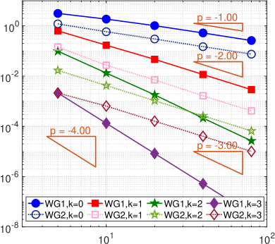
Refer to caption Refer to caption
(a) (b)
Fig. 16: Test 6.3.2. Convergence test for: (a) velocity error in ||||||{|||}\cdot{|||}-norm; (b) velocity error in L2superscript𝐿2L^{2}-norm.

7 Conclusion Remark

In this paper, we have developed a new stabilizer free and pressure-robust weak Galerkin scheme for solving Stokes equation on polygonal mesh. The new method modifies the right hand side assembling by projecting the test function into the H(div)-conforming space Λk(T)subscriptΛ𝑘𝑇\Lambda_{k}(T). This new method shows features of divergence preserving and robustness on viscosity variable ν𝜈\nu. Besides, the convergence test shows that one order superconvergence is obtained than the optimal order. the numerical performance can be significantly improved by using such techniques. Finally, the design of the reconstruction operator can be transferred into other polygonal finite element methods including HHO, HDG, and VEM methods.

The results in this paper can be applied to solve other incompressible flow, including Navier-Stokes equations and Brinkman equations, when the mass conservation is desired in the discretization. We shall include such applications in the future work plan.

References

  • [1] D.N. Arnold and D. Boffi and R.S. Falk, Quadrilateral H (div) finite elements, SIAM Journal on Numerical Analysis, 42 (2005): 2429-2451.
  • [2] L. Beirão da Veiga, F. Brezzi, A. Cangiani, G. Manzini, L. Marini, and A. Russo, Basic principles of virtual element methods, Math. Models Methods Appl. Sci. 23 (2013): 199-214.
  • [3] L. Beirão da Veiga, F. Brezzi, and L. Marini, Virtual elements for linear elasticity problems, SIAM J. Numer. Anal. 51 (2013): 794-812.
  • [4] D. Boffi and F. Brezzi and M. Fortin, Mixed finite element methods and applications, Heidelberg: Springer; 2013.
  • [5] C. Brennecke, A. Linke, C. Merdon, and J. Schöberl, Optimal and pressure-independent L2superscript𝐿2L^{2} velocity error estimates for a modified Crouzeix-Raviart Stokes element with BDM reconstructions, J. Comput. Math., 33 (2015): 191-208.
  • [6] F. Brezzi and M. Fortin, Mixed and Hybrid Finite Elements, Springer-Verlag, New York, 1991.
  • [7] W. Chen and Y. Wang, Minimal Degree H(curl) and H(div) conforming finite elements on polytopal meshes. Math. Comp. 86 (2017): 2053-2087.
  • [8] L. Chen, M. Wang, and L. Zhong, Convergence analysis of triangular MAC schmes for two dimensional Stokes equations, J. Sci. Comput. 63 (2015): 716-744.
  • [9] B. Cockburn, G. Kanschat, D. Schötzau, A note on discontinuous Galerkin divergence-free solutions of the Navier-Stokes equations, J. Sci. Comput. 31 (2007): 61-73.
  • [10] B. Cockburn, D. Di Pietro, and A. Ern, Bridging the hybrid high-order and hybridizable discontinuous Galerkin methods, ESAIM Math. Model. Numer. Anal., 50 (2016): 635-650.
  • [11] R. Falk and M. Neilan, Stokes complexes and the construction of stable finite elements with pointwise mass conservation, SIAM J. Numer. Anal. 51 (2013): 1308-1326.
  • [12] J. Guzmán and M. Neilan, Conforming and divergence free Stokes elements on general triangular meshes, Mathematics of Computation, 83 (2014): 15-36.
  • [13] J. Guzmán and M. Neilan, Conforming and divergence-free Stokes elements in three dimensions, IMA Journal of Numerical Analysis, 34 (2014): 1489-1508.
  • [14] E. Jenkins, V. John A. Linke, and L. Rebholz, On the parameter choice in grad-div stabilization for the Stokes equations, Adv. Compute. Math., 40 (2014): 491-516.
  • [15] V. John, A. Linke, C. Merdon, M. Neilan, and L. Rebholz, On the divergence constraint in mixed finite element mehtods for incompressible flows, SIAM Review.
  • [16] P. Lederer, Pressure-robust discretizations for Navier-Stokes equations: Divergence-free reconstruction for Taylor-Hood elements and high order Hybrid Discontinuous Galerkin methods, master’s thesis, Vienna Technical University, 2016.
  • [17] P. Lederer and J. Schöberl, Polynomial robust stability analysis for h(div)-conforming finite elements for the stokes equations, IMA Journal of Numerical Analysis, 38 (2018): 1832-1860.
  • [18] A. Linke, A divergence-free velocity reconstruction for incompressible flows, C. R. Math. Acad. Sci. Paris, 350 (2012): 837-840.
  • [19] A. Linke, On the role of the Helmholtz decomposition in mixed methods for incompressible flows and a new variational crime, Computer Methods in Applied Mechanics and Engineering, 268 (2014): 782-800.
  • [20] A. Linke, G. Matthies, and L. Tobiska, Robust arbitrary order mixed finite element methods for the incompressible Stokes equations with pressure independent velocity errors, ESAIM: M2AN, 50 (2016): 289-309.
  • [21] K. Lipnikov, G.  Manzini, M. Shashkov, Mimetic finite difference method, J. Comput. Phys. 257 (2014): 1163-1227.
  • [22] L. Mu, Pressure robust weak Galerkin Finite Element Methods for Stokes Problems, SIAM Journal on Scientific Computing, 42 (2020), B608–B629.
  • [23] M. Olshanskii and A. Olshanskii, Grad-div stabilization for Stokes equations, Math. Comp. 73 (2004): 1699-1718.
  • [24] M. Olshanskii, G. Lube, T. Heister, and J. Löwe, Grad-div stabilization and subgrid pressure models for the incompressible Navier-Stokes equations, Comput. Methods Appl. Mech. Engrg., 198 (2009): 3975-3988.
  • [25] D. Di Pietro, A. Ern, A hybrid high-order locking-free method for linear elasticity on general meshes, Comput. Methods Appl. Mech. Eng. 283 (2015): 1-21.
  • [26] L. Scott and M. Vogelius, Norm estimates for a maximal right inverse of the divergence operator in spaces of piecewise polynomials, ESAIM: M2AN 19 (1985): 111-143.
  • [27] J. Wang and X. Ye, New finite element methods in computational fluid dynamics by H(div) elements, SIAM J. Numer. Anal. 45 (2007): 1269-1286.
  • [28] S. Zhang, Divergence-free finite elements on tetrahedral grids for k6𝑘6k\geq 6, Math. Comput. 80 (2011): 669-695.
  • [29] D. Frerichs and C. Merdon, Divergence-preserving reconstructions on polygons and a really pressure-robust virtual element method for the Stokes problem, arXiv preprint, arXiv:2002.01830 (2020).
  • [30] J. Wang and X. Ye, A weak Galerkin finite element method for second-order elliptic problems. J. Comput. Appl. Math. 241 (2013), 103-115.
  • [31] J. Wang and X. Ye, A Weak Galerkin mixed finite element method for second-order elliptic problems, Math. Comp., 83 (2014), 2101-2126.
  • [32] X. Ye and S. Zhang, A stabilizer free weak Galerkin finite element method on polytopal mesh: Part II, arXiv:2008.13631.
  • [33] X. Ye and S. Zhang, A stabilizer free WG Method for the Stokes Equations with order two superconvergence on polytopal mesh, arXiv:2009.12226.