Statistical and Analytical Approaches
to Finite Temperature Magnetic Properties of SmFe₁₂ compound

Abstract

To investigate the magnetic properties of SmFe₁₂, we construct an effective spin model, where magnetic moments, crystal field (CF) parameters, and exchange fields at 0 K are determined by first principles. Finite temperature magnetic properties are investigated by using this model. We further develop an analytical method with strong mixing of states with different quantum number of angular momentum $J$ ($J$-mixing), which is caused by strong exchange field acting on spin component of $4f$ electrons. Comparing our analytical results with those calculated by Boltzmann statistics, we clarify that the previous analytical studies for Sm transition metal compounds over-estimate the $J$-mixing effects. The present method enables us to make quantitative analysis of temperature dependence of magnetic anisotropy (MA) with high-reliability. The analytical method with model approximations reveals that the $J$-mixing caused by exchange field increases spin angular momentum, which enhances the absolute value of orbital angular momentum and MA constants via spin-orbit interaction. It is also clarified that these $J$-mixing effects remain even above room temperature. Magnetization of SmFe₁₂ shows peculiar field dependence known as first-order magnetization process (FOMP), where the magnetization shows an abrupt change at certain magnetic field. The result of the analysis shows that the origin of FOMP is attributed to competitive MA constants between positive $K_{1}$ and negative $K_{2}$. The sign of $K_{1(2)}$ appears due to an increase in CF potential denoted by the parameter $A_{2}^{0}\langle r^{2}\rangle$ ($A_{4}^{0}\langle r^{4}\rangle$) caused by hybridization between $3d$-electrons of Fe on $8i$ ($8j$) site and $5d$ and $6p$ valence electrons on Sm site. It is verified that the requirement for the appearance of FOMP is given as $-K_{2}<K_{1}<-6K_{2}$.

I Introduction

There have been intensive studies on developing new rare-earth ($R$) lean permanent magnetic materials which have strong magnetic properties comparable to those of Nd-Fe-B. Nitrogenated compounds as NdFe₁₂N or NdFe₁₁TiN have been considered to be candidates of such materials, and thus series of experimental and theoretical efforts have been made to figure out the magnetic properties of these materials Miyake ; Hirayama1 . SmFe₁₂ with the ThMn₁₂ structure (Fig. 1) is also a possible candidate and has attracted renewed interest because it exhibits excellent intrinsic magnetic properties such as uniaxial magnetocrystalline anisotropy Hadjipanayis . Although SmFe₁₂ itself is thermodynamically unstable, it has been known that the substitution of Fe with a stabilizing element, such as Ti or V, can remove this difficulty Ohashi1 ; Ohashi2 ; Hu ; Kuno ; Schoenhoebel . In these systems, however, the saturated magnetization is reduced due to anti-parallel alignment of magnetic moments of Ti and V relative to those of Fe. Recent development of the synthesis technology made it possible to fabricate highly textured single phase samples of SmFe₁₂ thin film Kato ; Hirayama2 ; Ogawa1 ; Ogawa2 ; Sepehri-Amin3 , and it has been shown experimentally that Co substitution for Fe enhances their magnetic properties, such as Curie temperature and magnetic anisotropy (MA) Hirayama2 . Thus, SmFe₁₂-based systems belong to one of the most promising hard magnetic materials, and therefore to clarify the basic magnetic properties of SmFe₁₂ is crucially important.

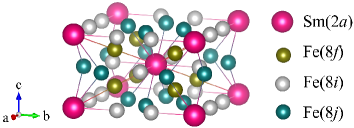
Figure 1: (color online) Crystal structure of SmFe₁₂ compound in ThMn₁₂ structure. Inequivalent sites: Sm(2$a$), Fe(8$f$), Fe(8$i$), and Fe(8$j$) are shown by different-colored balls and solid lines show interatomic short contacts less than 3.2 Å.

So far many attempts have been performed for microscopic understanding of the magnetic properties of $R$ based permanent magnets Evans ; Toga ; Nishino ; MiyakeAkai ; Yoshioka ; Tsuchiura2 . Among them a powerful method is to combine the first-principle calculations for electronic states at the ground state with a suitable model for finite temperature properties Yamada ; Sasaki ; Miura-direct ; Miura-pl ; Kuzminlinear ; Kuzmin2nd ; Kuzminlimit ; Millev ; Kuzminmix ; Magnani . As for SmFe₁₂, Harashima et al. (2015) Harashima , Körner et al (2016) Koerner and Delonge et al (2017) Delange performed the first-principle calculations and model analysis of magnetic properties. In the theoretical study of Sm-based intermetallic compounds, however, there remains a basic issue how to deal with the formidably strong $J$-mixing effects in Sm. This is the problem studied for a long period on the Sm-based magnets VanVleck ; Sankar ; Wijin . There are some attempts to include the $J$-mixing in the analytical form by the first-order perturbation for the crystal fields (CFs) Kuzminmix ; Magnani . However, Kuz’min pointed out that the Sm-based magnetic materials are exceptional for application of the method Kuzminmix .

We have recently developed a similar method Yoshioka ; Tsuchiura2 , in which the model parameters are calculated by the first-principles and the finite temperature magnetic properties are calculated in a statistical way, and applied it to $R_{2}$Fe₁₄B systems. By taking into account CF parameters up to 6-th order, the model satisfactorily explained the experimental results for magnetization curves and the temperature dependence of MA constants Yoshioka ; Tsuchiura2 . Using the method we recently calculated the temperature dependence of the MA constants of SmFe₁₂ and showed that $K_{1}>0$ and $K_{2}<0$ in consistence with experimental results Ogawa2 . The report of the work, however, contains only the final results and no details of computational procedure have been presented. As a results no explanations on the mechanism for the results that $K_{1}>0$ and $K_{2}<0$ have been given.

The purpose of the present study is thus to clarify the origin of the finite temperature magnetic properties of SmFe₁₂ compound by statistical and analytical ways. To this end, we describe the details of the statistical method and develop a novel analytical method. The analytical procedure is able to derive simple relations between the temperature dependence of magnetic properties and parameters determined by first-principles electronic structure calculations. The treatment of the $J$-mixing effects adopted previously by the other groups Kuzminmix ; Magnani will be modified, and the results will be compared with the statistical results of the temperature dependence of magnetic properties of SmFe₁₂. Good agreement between the analytical and statistical results guarantees the applicability of the modified analytical formula to Sm compounds.

In the following, we give the model Hamiltonian, the parameters of which are determined by the first-principles, and present the calculation procedure for finite temperatures, especially the statistical method to obtain the MA constants and magnetization curves, and explain the modified analytical method. The latter method may clarify the relations among the free energy of the system, the CF, and the exchange field. Using the analytical method, we will show that the mechanism of $K_{1}>0$ and $K_{2}<0$ in SmFe₁₂ is attributed to the characteristic lattice structure around Sm ions, that is, crystallographic 2$b$-sites on $c$-axis adjacent to Sm are vacant. We also present results on the magnetization process and nucleation fields by calculating Gibbs free energy. As pointed out in Ref. Tsuchiura2 , this analytical spin model can be easily extended to Sm ions around the intergranular phases, which is crucially important in the coercivity mechanism Sepehri-Amin1 ; Sepehri-Amin2 ; Sepehri-Amin3 .

This paper is organized as follows. The model Hamiltonian is explained in Section II, and the procedure of the statistical and analytical method are explained in Section III. Section IV shows the results of temperature dependence of magnetic properties calculated in the statistical and analytical methods. A summary of our work is given in Section V.

II Model Hamiltonian

We adopt a following Hamiltonian to investigate the magnetic properties of $R$ transition metal ($TM$) compounds:

$$\hat{\cal H}= \frac{1}{V_{0}}\sum_{j=1}^{n_{R}}\hat{\cal H}_{R,j}$$

$$+K_{1}^{TM}(T)\sin^{2}\theta^{TM}-{\bm{M}}^{TM}(T)\cdot{\bm{B}},$$ (1)

where $\hat{\cal H}_{R,j}$ is a Hamiltonian for $R$ ion on $j$-th site and $n_{R}$ is the number of $R$ ion in the unit cell volume $V_{0}$. Second and third term represent the phenomenological treatment of MA energy and Zeeman term on $TM$ sublattice, where $K_{1}^{TM}(T)$ and ${\bm{M}}^{TM}(T)$ are the temperature dependent anisotropy constant and magnetization vector of $TM$ sublattice, respectively, and $\theta^{TM}$ is the polar angle of ${\bm{M}}^{TM}(T)$ against the $c$-axis. ${\bm{M}}^{TM}(T)$ is given as $M^{TM}(T){\bm{e}}^{TM}$ by using the absolute value of the sublattice magnetization $M^{TM}(T)$ and a directional vector ${\bm{e}}^{TM}$ of ${\bm{M}}^{TM}(T)$. $M^{TM}(T)$ is defined by a part of magnetization subtracting the $4f$ electron contribution from the total magnetization. ${\bm{B}}$ is an applied field.

II.1 Hamiltonian of Single $R$ Ion

The Hamiltonian for $4f$ shell in $j$-th $R$ ion in Eq. (1) is

$$\hat{\cal H}_{R,j} =\sum_{i=1}^{n_{4f}}\hat{h}_{j}(i)+\frac{1}{8\pi\varepsilon_{0}}\sum_{i\neq i^{\prime}=1}^{n_{4f}}\frac{e^{2}}{|\hat{\bm{r}}_{i}-\hat{\bm{r}}_{i^{\prime}}|},$$ (2)

with

$$\hat{h}_{j}(i)= \xi\hat{\bm{l}}_{i}\cdot\hat{\bm{s}}_{i}+2\mu_{B}\hat{\bm{s}}_{i}\cdot{\bm{B}}_{{\rm ex},j}(T)$$

$$+\int r_{i}^{2}|R_{4f}(r_{i})|^{2}V_{j}({\bm{r}}_{i})dr_{i}$$

$$+\mu_{B}(\hat{\bm{l}}_{i}+2\hat{\bm{s}}_{i})\cdot{\bm{B}}.$$ (3)

The first and second terms in Eq. (2) represent the single electron contribution and the electron-electron repulsion in $4f$ shell, respectively, where $n_{4f}$ is the number of $4f$ electrons, $\varepsilon_{0}$ and $e$ are the vacuum permittivity and the elementary charge, respectively. $\hat{h}_{j}(i)$ in Eq. (3) is the Hamiltonian for $i$-th $4f$ electron on $j$-th $R$ site, where the first term in Eq. (3) is the spin-orbit interaction (SOI) between spin ($\hat{\bm{s}}_{i}$) and orbital ($\hat{{\bm{l}}_{i}}$) angular momenta, with a coupling constant $\xi$. The second term represents the exchange interaction between spin moment and temperature dependent exchange field ${\bm{B}}_{{\rm ex},j}(T)=-{\bm{e}}^{TM}B_{{\rm ex},j}(T)$ on $j$-th $R$ site, where $\mu_{B}$ is the Bohr magneton. The third and fourth terms are the CF and Zeeman terms, respectively. In the expression of CF, $V_{j}({\bm{r}}_{i})$ and $R_{4f}(r_{i})$ are Coulomb potential and radial parts of the $4f$ wave function on $j$-th $R$ site, respectively. Note that the kinetic energy and screened central potential terms are effectively taken into account in the formation of $4f$ orbital.

To obtain the electronic properties at $T=0$, we apply the first-principles and determine the parameters in the Hamiltonians in Eq. (3). We use the full-potential linearized augmented plane wave plus local orbitals (APW+lo) method implemented in the WIEN2k code wien2k . The Kohn-Sham equations are solved within the generalized-gradient approximation (GGA). To simulate localized $4f$ states, we treat $4f$ states as atomic-like core states, which is so called opencore method Richter1 ; Novak ; Hummler0 ; Richter2 ; Divis1 ; Divis2 .

We calculate the ground state properties of SmFe₁₂ such as Coulomb potential, charge distribution, and sublattice magnetizations. In accord with the previous theoretical studies for SmFe₁₂ Harashima ; Koerner ; Delange , we assume that Sm ion has trivalent-like electronic structure. The exchange fields $B_{{\rm ex},j}(0)$ at $T=0$ are determined from an energy increase caused by spin flip of $4f$ electrons Brooks ; Yoshioka , and CFs acting on $i$-th $4f$ electron are directly estimated from Coulomb potential $V_{j}({\bm{r}}_{i})$ acting on $j$-th $R$ site. It is noted that the single ion Hamiltonian $\hat{\cal H}_{R,j}$ thus determined for $j$-th $R$ ions includes effects of $TM$ atoms surrounding the $R$ ions as a mean field.

Practically, the CF term is rewritten as the following formula Novak ; Richter2 :

$$\int_{0}^{r_{c}}r_{i}^{2}|R_{4f}(r_{i})|^{2} V_{j}({\bm{r}}_{i})dr_{i}=\sum_{l,m}\frac{A_{l,j}^{m}\langle r^{l}\rangle}{a_{l,m}}t_{l}^{m}(\hat{\theta}_{i},\hat{\varphi}_{i}),$$ (4)

$$A_{l,j}^{m}\langle r^{l}\rangle= a_{l,m}\int_{0}^{r_{\rm c}}dr_{i}r_{i}^{2}|R_{4f}(r_{i})|^{2}$$

$$\times\int d\Omega_{i}V_{j}({\bm{r}}_{i})t_{l}^{m}(\theta_{i},\varphi_{i}),$$ (5)

where $A_{l,j}^{m}\langle r^{l}\rangle$ is CF parameter on $j$-th $R$ site, $a_{l,m}$ is a numerical factor Hutchings , $t_{l}^{m}(\hat{\theta}_{i},\hat{\varphi}_{i})$ is tesseral harmonic function of a solid angle $\Omega=(\hat{\theta}_{i},\hat{\varphi}_{i})$, and $r_{\rm c}$ is a cut-off radius.

Values of CF parameters $A_{l,j}^{m}\langle r^{l}\rangle$ in Eq. (5), exchange field $B_{{\rm ex},j}(0)$ in Eq. (3), $TM$-sublattice magnetization $M^{TM}(0)$ in Eq. (1) in SmFe₁₂ are shown in TABLE 1. The lattice constants used in this calculations are the experimental values $a=b=8.35$ Å and $c=4.8$ Å Hirayama2 . For Wycoff positions, we apply the theoretically optimized ones given in Ref. Harashima . The crystal structure of SmFe₁₂ is shown in Fig. 1.

Table 1: Values of CF potentials $A_{l,j}^{m}\langle r^{l}\rangle$ [K], exchange field $\mu_{\rm B}B_{{\rm ex},j}(0)/k_{\rm B}$ [K], and $TM$-sublattice magnetization $V_{0}M^{TM}(0)$ [$\mu_{\rm B}$] in SmFe₁₂ calculated by first-principles, where $\mu_{\rm B}$ and $k_{\rm B}$ are Bohr magneton and Boltzmann constant, respectively, and $V_{0}=a\times b\times c$. We note that $A_{l,j}^{m}\langle r^{l}\rangle$ and $\mu_{\rm B}B_{{\rm ex},j}(0)/k_{\rm B}$ are independent of site index $j$.

$A_{2,j}^{0}\langle r^{2}\rangle$	$A_{4,j}^{0}\langle r^{4}\rangle$	$A_{4,j}^{4}\langle r^{4}\rangle$	$A_{6,j}^{0}\langle r^{6}\rangle$	$A_{6,j}^{4}\langle r^{6}\rangle$	$\mu_{\rm B}B_{{\rm ex},j}(0)/k_{\rm B}$	$V_{0}M^{TM}$(0)
-71.4	-21.3	-49.3	5.9	3.0	296.1	51.6

II.2 Single $R$ Ion Hamiltonian
in $LS$ Coupling Regime

We here apply the concept of $LS$ coupling to the single electron Hamiltonian of Eq. (3) with Russell Saunders states $|L,S;J,M\rangle$, due to the strong Coulomb interaction between $4f$ electrons. According to the Hund’s rule, we specify the quantum number of total orbital (spin) moment $L(S)$. Total angular momentum $J$ is varied from $|L-S|$ to $L+S$, and $M$ is the magnetic quantum number. Thus the single ion Hamiltonian in Eq. (2) can be reduced to:

$$\hat{\cal H}_{R} =\hat{\cal H}_{{\rm so}}+\hat{\cal H}_{\rm ex}+\hat{\cal H}_{\rm CF}+\hat{\cal H}_{\rm Z},$$ (6)

$$\hat{\cal H}_{\rm so} =\lambda\hat{\bm{L}}\cdot\hat{\bm{S}},$$ (7)

$$\hat{\cal H}_{\rm ex} =2\mu_{\rm B}\hat{\bm{S}}\cdot{\bm{B}}_{\rm ex}(T),$$ (8)

$$\hat{\cal H}_{\rm CF} =\sum_{l,m,m^{\prime}}B_{l}^{m}\Theta_{l}^{L}C_{m}^{(l)}(\hat{\bm{L}}),$$ (9)

$$\hat{\cal H}_{\rm Z} =\mu_{\rm B}(\hat{\bm{L}}+2\hat{\bm{S}})\cdot{\bm{B}}.$$ (10)

Hereafter, the site index $j$ is omitted for single-ion quantity. $\hat{\bm{L}}$ and $\hat{\bm{S}}$ are total orbital and spin momenta of $4f$ electrons, respectively, $B_{l}^{0}=\sqrt{(2l+1)/4\pi}A_{l}^{0}\langle r^{l}\rangle/a_{l,0}$ and $B_{l}^{\pm|m|}=(\mp 1)^{m}\sqrt{(2l+1)/8\pi}\left[A_{l}^{|m|}\langle r^{l}\rangle\mp iA_{l}^{-|m|}\langle r^{l}\rangle\right]/a_{l,m}$ for $m\neq 0$, and $\Theta_{l}^{L}=\langle L\parallel\sum_{i}C^{(l)}_{m}(\hat{\theta}_{i},\hat{\varphi}_{i})\parallel L\rangle/\langle L\parallel\sum_{i}C^{(l)}_{m}(\hat{\bm{L}})\parallel L\rangle$. In the treatment of SOI, we should note that the eigenstates of $LS$ coupling are specified by the quantum number of $J$. In general, the term $\hat{\cal H}_{\rm so}$ is dominating in Eq. (6). Thus $J$ is a good quantum number in most of the $R$-$4f$ systems. Because the $LS$ coupling in Sm compounds is weak compared with other $R$ ones, it is necessary to include excited $J$-multiplets. Hereafter, we abbreviate the states $|L,S;J,M\rangle$ as $|J,M\rangle$.

Figure 2: Energy levels as a function of $B_{\rm ex}(T)/B_{\rm ex}(0)$ of the Sm-$4f$ states in SmFe₁₂ at ${\bm{e}}^{TM}={\bm{n}}_{c}$ and for ${\bm{B}}={\bm{0}}$. High energy levels originated from $J=13/2$ and $J=15/2$ multiplets are above 6000 K, which are not shown.

The energy levels of Sm-$4f$ states in SmFe₁₂ depend on ${\bm{B}}_{\rm ex}(T)$ and applied field ${\bm{B}}$. Fig. 2 shows the $B_{\rm ex}(T)/B_{\rm ex}(0)$ dependence of the energy levels for ${\bm{e}}^{TM}$=${\bm{n}}_{c}$, which is a unit vector parallel to $c$-axis, and for ${\bm{B}}={\bm{0}}$. The data needed are given in TABLE 1. As for SOI constant, we use experimental value of $\lambda/k_{B}=\xi/5k_{B}=411$ K Elliott . At $B_{\rm ex}(T)=0$ the $S$ is strongly coupled with $L$ to form a Kramers doublet with a total angular momentum $J$ due to the large $LS$ coupling with fine CF splitting. With increasing $B_{\rm ex}(T)/B_{\rm ex}(0)$, the exchange field breaks the time-reversal symmetry and lift the degeneracy.

II.3 Phenomenological Model for $TM$ Sublattice

For finite temperature magnetic properties of TM, we apply a phenomenological formula assuming uniform $M^{TM}(T)$ and $K_{1}^{TM}(T)$. For $M^{TM}(T)$, we apply the Kuz’min formula Kuzminmag :

$$\frac{M^{TM}(T)}{M^{TM}(0)} =\frac{B_{\rm ex}(T)}{B_{\rm ex}(0)}=\alpha(T),$$ (11)

$$\alpha(T) =\left[1-s\left(\frac{T}{T_{\rm C}}\right)^{3/2}-(1-s)\left(\frac{T}{T_{\rm C}}\right)^{5/2}\right]^{1/3},$$ (12)

where, $T_{\rm C}$ is Curie temperature and $s$ is a fitting parameter. The temperature dependence of $K_{1}^{TM}(T)$ has been expressed by an extended power law Miura-pl :

$$\frac{K_{1}^{TM}(T)}{K_{1}^{TM}(0)}= \alpha^{3}(T)+\frac{8}{7}C_{1}\left[\alpha^{3}(T)-\alpha^{10}(T)\right]$$

$$+\frac{8}{7}C_{2}\left[\alpha(T)^{3}-\frac{18}{11}\alpha(T)^{10}+\frac{7}{11}\alpha(T)^{21}\right],$$ (13)

where $C_{1}$ and $C_{2}$ are fitting parameters.

In present study for SmFe₁₂ compound, we use values of $s=0.01$ and $T_{\rm C}=555$ K in Eq. (12), as used by Hirayama $et$ $al$. Hirayama2 . They showed that the magnetization agrees well with experimental measurement for SmFe₁₂. The values of $C_{1}$, $C_{2}$ and $V_{0}K_{1}^{TM}(0)$ in Eq. (13) are determined as $-0.263$, $-0.237$ and $47.7$ K, respectively, by fitting the expression to observed data for YFe₁₁Ti in Ref. Nikitin .

III Method of Model Calculations

III.1 Statistical Method

To calculate the finite temperature magnetic properties, we use the model Hamiltonian and calculate MA and magnetic moment for Sm $4f$ electrons using the statistical method for the partial system. Using the eigenvalues of the Hamiltonian Eq. (6), we express the free energy density as,

$$G({\bm{e}}^{TM},T,{\bm{B}})= \frac{1}{V_{0}}\sum_{j=1}^{n_{R}}g_{j}({\bm{e}}^{TM},T,{\bm{B}})$$

$$+K_{1}^{TM}(T)\sin^{2}\theta^{TM}-{\bm{B}}\cdot{\bm{M}}^{TM}(T),$$ (14)

$$g_{j}({\bm{e}}^{TM},T,{\bm{B}})= -k_{\rm B}T\ln Z_{j}({\bm{e}}^{TM},T,{\bm{B}}),$$ (15)

$$Z_{j}({\bm{e}}^{TM},T,{\bm{B}})= \sum_{n}\exp\left[-\frac{E_{n,j}({\bm{e}}^{TM},T,{\bm{B}})}{k_{\rm B}T}\right],$$ (16)

where $g_{j}({\bm{e}}^{TM},T,{\bm{B}})$ is Gibbs free energy for $R$-$4f$ partial system, $E_{n,j}({\bm{e}}^{TM},T,{\bm{B}})$ and $Z_{j}({\bm{e}}^{TM},T,{\bm{B}})$ are the eigenvalue and the partition function of $j$-th $R$ Hamiltonian $\hat{\cal H}_{R,j}$ [Eq. (6)] for given ${\bm{e}}^{TM}$, respectively. The direction of the $TM$ magnetization ${\bm{e}}^{TM}$ is treated as an external parameter. The equilibrium condition of the system for given $T$ and $\bm{B}$ is:

$$G({\bm{e}}_{0}^{TM},T,{\bm{B}})=\min_{{\bm{e}}^{TM}}G({\bm{e}}^{TM},T,{\bm{B}}),$$ (17)

where ${\bm{e}}_{0}^{TM}$ is the direction of $TM$ sublattice magnetization in the equilibrium. In practice, we determine the minimal $G({\bm{e}}^{TM},T,{\bm{B}})$ numerically by changing ${\bm{e}}^{TM}$.

The MA energy is given by the free energy $G({\bm{e}}^{TM},T,{\bm{0}})$ with different directional vector ${\bm{e}}^{TM}$. In the tetragonal symmetry, $g_{j}({\bm{e}}^{TM},T,{\bm{0}})$ in $G({\bm{e}}^{TM},T,{\bm{0}})$ is formally expressed as Kuzminlinear ; Miura-pl :

$$g_{j}({\bm{e}}^{TM},T,{\bm{0}})= \sum_{p=1}^{\infty}\left[k_{p,j}(T)+\sum_{q=1}^{\lfloor p/2\rfloor}k_{p,j}^{q}(T)\cos(4q\varphi^{TM})\right]$$

$$\times\sin^{2p}\theta^{TM}+C(T),$$ (18)

where $\theta^{TM}$ and $\varphi^{TM}$ are polar and azimuthal angle of ${\bm{e}}^{TM}$, respectively, $\lfloor p/2\rfloor$ indicates the greatest integer of $p/2$, and $k_{p,j}(T)$ and $k_{p,j}^{q}(T)$ are out-of-plane and in-plane MA constant for $j$-th $R$ ion. The $C(T)$ is an angle independent constant. The series expansion does not guarantee the convergence Kuzmin2nd ; Kuzminlimit , however, for finite $p$, $k_{p,j}^{q}(T)$ can be obtained from the comparison between Taylor series of $g_{j}({\bm{e}}^{TM},T,{\bm{0}})$ of Eqs. (15) and (18) with respect to $\theta^{TM}$ for a fixed $\varphi^{TM}$ Sasaki ; Miura-direct as:

$$g_{j}({\bm{e}}^{TM},T,{\bm{0}})= g_{j}^{(0)}(T)+g_{j}^{(1)}(T)\theta^{TM}$$

$$+\frac{1}{2!}g_{j}^{(2)}(T)(\theta^{TM})^{2}+\cdots,$$

$$g_{j}^{(n)}(T)= \left.\frac{\partial^{n}g_{j}(\theta^{TM},\varphi^{TM},T,{\bm{0}})}{\partial(\theta^{TM})^{n}}\right|_{\begin{subarray}{c}\theta^{TM}=0,\\ \varphi^{TM}=\pi/8\end{subarray}},$$

and

$$g_{j}({\bm{e}}^{TM},T,{\bm{0}})= k_{1,j}(T)(\theta^{TM})^{2}$$

$$+\left[-\frac{2}{3!}k_{1,j}(T)+k_{2,j}(T)\right](\theta^{TM})^{4}+\cdots,$$

respectively, which are resulting in

$$k_{1,j}(T) =\frac{1}{2}g_{j}^{(2)}(T),$$ (19)

$$k_{2,j}(T) =\frac{1}{3}k_{1,j}(T)+\frac{1}{4!}g_{j}^{(4)}(T),$$ (20)

etc. Using MA energy on the single $R$ ion in Eq. (18), the total MA constants are obtained as

$$K_{1}(T) =\frac{1}{V_{0}}\sum_{j=1}^{n_{R}}k_{1,j}(T)+K_{1}^{TM}(T), (p=1),$$ (21)

$$K^{(q)}_{p}(T) =\frac{1}{V_{0}}\sum_{j=1}^{n_{R}}k_{p,j}^{(q)}(T), (p\geq 2),$$ (22)

where $K_{p}(T)$ and $K_{p}^{q}(T)$ are out-of-plane and in-plane MA constant in whole system.

The orbital and spin components of the magnetic moment of a single $R$ ion in the equilibrium, can be calculated by:

$${\bm{m}}_{L,j}(T,{\bm{B}}) =-\mu_{\rm B}\sum_{n}\rho_{n,j}(T,{\bm{B}})\langle n,j|{\hat{\bm{L}}}|n,j\rangle,$$ (23)

$${\bm{m}}_{S,j}(T,{\bm{B}}) =-2\mu_{\rm B}\sum_{n}\rho_{n,j}(T,{\bm{B}})\langle n,j|{\hat{\bm{S}}}|n,j\rangle,$$ (24)

respectively, where $\rho_{n,j}(T,{\bm{B}})=\exp\left[-\beta E_{n,j}({\bm{e}}^{TM}_{0},{\bm{B}})\right]/Z_{j}({\bm{e}}^{TM}_{0},T,{\bm{B}})$ and $|n,j\rangle$ is the $n$-th eigenstate for $E_{n,j}({\bm{e}}_{0}^{TM},{\bm{B}})$, and the total magnetization $M_{\rm s}(T,{\bm{B}})$ is given as,

$${\bm{M}}_{\rm s}(T,{\bm{B}}) =\frac{1}{V_{0}}\sum_{j=1}^{n_{R}}{\bm{m}}_{j}(T,{\bm{B}})+M^{TM}(T){\bm{e}}_{0}^{TM},$$ (25)

with ${\bm{m}}_{j}(T,{\bm{B}})={\bm{m}}_{L,j}(T,{\bm{B}})+{\bm{m}}_{S,j}(T,{\bm{B}})$.

Finally, to confirm the convergence of the probability weights for excited-$J$ multiplet states at ${\bm{B}}={\bm{0}}$, we define a following weight function:

$$W_{J}(T)=\sum_{n,M}\rho_{n,j}(T,{\bm{0}})|\langle n,j|J,M\rangle|^{2}.$$ (26)

In the case of SmFe₁₂ crystal, the value of $W_{J}(T)$ is independent of site index $j$.

Table 2: Probability weight for each $J$-multiplet calculated by $W_{J}(T)$ in Eq. (26). For $J=13/2$ and $15/2$, $W_{J}(T)=0.0$.

$J$	5/2	7/2	9/2	11/2
$T$=0	0.93217	0.06548	0.00229	0.00005
$T=T_{\rm C}$	0.90536	0.09049	0.00406	0.00009

The results are shown in TABLE 2, which indicates good convergence of weight for the number of the excited $J$-multiplets even at $T=T_{\rm C}=555$ K. Thus in the calculation using statistical method for SmFe₁₂, we take the excited $J$-multiplets up to $J=9/2$. In the analytical calculation, the $J$-mixing effects are approximately treated only for the lowest-$J$ multiplet by using unitary transformation.

III.2 Analytical Method

According to hierarchy of energy scale in $R$ intermetallic compounds: $\hat{\cal H}_{\rm so}\gg\hat{\cal H}_{\rm ex}\gg\hat{\cal H}_{\rm CF}\sim\hat{\cal H}_{\rm Z}$, we develop an analytical method for finite temperature magnetic properties, which enables us to connect the thermodynamic properties directly to our model parameters based on electronic states. Practically, we generalize the analytical expression of Gibbs free energy Yamada ; Kuzminlinear to include the effects of $J$-mixing using a first-order perturbation for the CF potential and Zeeman energy. We also derive an analytical expression for the magnetization curve, which enables us to estimate the CF potential using the observed results. The procedure of the formalism consists of (i) construction of starting Hamiltonian for single $R$ ion, (ii) approximation for diagonal matrix element of an effective Hamiltonian, (iii) finite temperature perturbation for single $R$ ion, and (iv) thermodynamic analysis.

III.2.1 Effective Lowest-$J$ Multiplet Hamiltonian
for Single $R$ Ion

To restrict $\hat{\cal H}_{R}$ in low-energy subspace for $\hat{\cal H}_{\rm so}\gg\hat{\cal H}_{\rm ex}$, the effective lowest-$J$ multiplet Hamiltonian $\hat{\cal H}_{R}^{{\rm eff}J}$ is obtained by unitary transformation and projection, where the off-diagonal matrix elements between inter-$J$ multiplets become negligibly small, and compensating term $\hat{\cal H}_{\rm mix}$ is added in diagonal element for lowest-$J$ multiplet. We here introduce modified version of effective Hamiltonian as explained below.

First, we define a rotational operator $\hat{\cal D}({\bm{e}}^{TM})$ which transforms the quantization axis to ${\bm{e}}^{TM}$. With this operator, the Hamiltonian $\hat{\cal H}_{R}$ and $\hat{\cal H}_{A}$ ($A$=ex, CF and Z) is transformed to:

$$\hat{\cal D}^{\dagger}({\bm{e}}^{TM} )\hat{\cal H}_{R}\hat{\cal D}({\bm{e}}^{TM})$$

$$\equiv\hat{\cal H}_{R}^{\prime}=\hat{\cal H}_{\rm so}^{\prime}+\hat{\cal H}_{\rm ex}^{\prime}+\hat{\cal H}_{\rm CF}^{\prime}+\hat{\cal H}_{\rm Z}^{\prime},$$ (27)

$$\hat{\cal H}_{\rm so}^{\prime}= \frac{\lambda}{2}\left[\hat{\bm{J}}^{2}-L(L+1)-S(S+1)\right],$$ (28)

$$\hat{\cal H}_{\rm ex}^{\prime}= -2B_{\rm ex}(T)C_{0}^{(1)}(\hat{\bm{S}}),$$ (29)

$$\hat{\cal H}_{\rm CF}^{\prime}= \sum_{l,m,m^{\prime}}B_{l}^{m}\Theta_{l}^{L}[{\cal D}_{m,m^{\prime}}^{(l)}({\bm{e}}^{TM})]^{\ast}C_{m^{\prime}}^{(l)}(\hat{\bm{L}}),$$ (30)

$$\hat{\cal H}_{\rm Z}^{\prime}= \mu_{\rm B}\sum_{m,m^{\prime}}b_{-m}^{(1)}[{\cal D}_{m,m^{\prime}}^{(1)}({\bm{e}}^{TM})]^{\ast}\left[C_{m^{\prime}}^{(1)}(\hat{\bm{L}})+2C_{m^{\prime}}^{(1)}(\hat{\bm{S}})\right],$$ (31)

where $\hat{\bm{J}}=\hat{\bm{L}}+\hat{\bm{S}}$, $C_{q}^{(k)}(\hat{\bm{A}})$ is the spherical tensor operator with rank $k$ for angular momentum $\hat{\bm{A}}$ Edomonds , and $b_{m}^{(1)}$ is a magnetic field tensor: $b_{0}^{(1)}=B_{z}$ and $b_{\pm 1}^{(1)}=-(\pm B_{x}+iB_{y})/\sqrt{2}$. ${\cal D}_{m,m^{\prime}}^{(l)}({\bm{e}}^{TM})={\cal D}_{m,m^{\prime}}^{(l)}(\varphi^{TM},\theta^{TM},0)$ is the Wigner’s $D$ function. Now we apply a unitary transformation (Schrieffer-Wolf transformation Schrieffer ) to $\hat{\cal H}_{R}^{\prime}$,

$$e^{i\hat{\Omega}}\hat{\cal H}_{R}^{\prime}e^{-i\hat{\Omega}}=\hat{\cal H}_{R}^{\prime}+i\left[\hat{\Omega},\hat{\cal H}_{R}^{\prime}\right]+O(\hat{\Omega}^{2}),$$ (32)

and introduce a projection operator $\hat{\cal P}_{J}=\sum_{M=-J}^{J}|J,M\rangle\langle J,M|$, by which the space of the $J$-multiplet is restricted to the lowest one. The operator $\hat{\Omega}$ is defined so as to remove the first-order off-diagonal matrix elements for $J$ in $\hat{\cal H}_{R}^{\prime}$:

$$i\sum_{J^{\prime}}\left[\hat{\Omega},\hat{\cal P}_{J^{\prime}}\hat{\cal H}_{R}^{\prime}\hat{\cal P}_{J^{\prime}}\right]=\sum_{J^{\prime}}\hat{\cal P}_{J^{\prime}}\hat{\cal H}_{R}^{\prime}\hat{\cal P}_{J^{\prime}}-\hat{\cal H}_{R}^{\prime}.$$ (33)

Apparently, $\langle J,M|\hat{\Omega}|J,M^{\prime}\rangle=0$. The second term of the right-hand-side of Eq. (32) has now a diagonal matrix with corrections to the diagonal elements in the original $\hat{\cal H}_{R}^{\prime}$. The second and higher-order terms in $\hat{\Omega}$ are neglected. By inserting Eq. (33) to Eq. (32), we obtain

$$\hat{\cal H}_{R}^{{\rm eff}J}= \hat{\cal P}_{J}e^{i\hat{\Omega}}\hat{\cal H}_{R}^{\prime}e^{-i\hat{\Omega}}\hat{\cal P}_{J}\equiv\hat{\cal H}_{R}^{J}+\hat{\cal H}_{\rm mix},$$ (34)

$$\hat{\cal H}_{R}^{J}= \hat{\cal P}_{J}\hat{\cal H}_{R}^{\prime}\hat{\cal P}_{J}=E_{J}+\hat{\cal H}_{\rm ex}^{J}+\hat{\cal H}_{\rm CF}^{J}+\hat{\cal H}_{\rm Z}^{J},$$ (35)

$$\hat{\cal H}_{\rm mix}= \frac{i}{2}\hat{\cal P}_{J}\left[\hat{\Omega},\hat{\cal H}_{R}^{\prime}\right]\hat{\cal P}_{J},$$ (36)

where $E_{J}=\lambda[J(J+1)-L(L+1)-S(S+1)]/2$ and $\hat{\cal H}_{A}^{J}=\hat{\cal P}_{J}\hat{\cal H}_{A}^{\prime}\hat{\cal P}_{J}$ ($A$=ex, CF and Z). We here classify analytical models depending on the approximation to the matrix element of $\hat{\Omega}$ for $J\neq J^{\prime}$ in Eq. (33) as follows:

• model A: Lowest-$J$ multiplet without mixing as:
  

  $$\langle J,M|\hat{\Omega}^{\rm A}|J^{\prime},M^{\prime}\rangle=0,$$

• model B: Effective lowest-$J$ multiplet with mixing as:
  

  $$\langle J,M|\hat{\Omega}^{\rm B}|J^{\prime},M^{\prime}\rangle=i\frac{\langle J,M|\hat{\cal H}_{1}|J^{\prime},M^{\prime}\rangle}{E_{J^{\prime}}-E_{J}},$$

• model C: Modified effective lowest-$J$ multiplet with mixing (present study) as:.

  $$\langle J,M| \hat{\Omega}^{\rm C}|J^{\prime},M^{\prime}\rangle$$

  $$= i\frac{\langle J,M|\hat{\cal H}_{1}|J^{\prime},M^{\prime}\rangle}{E_{J^{\prime}}-E_{J}}-\frac{i}{(E_{J^{\prime}}-E_{J})^{2}}$$

  $$\times\sum_{M^{\prime\prime}}\left[\langle J,M|\hat{\cal H}_{1}|J^{\prime},M^{\prime\prime}\rangle\langle J^{\prime},M^{\prime\prime}|\hat{\cal H}_{1}|J^{\prime},M^{\prime}\rangle\right.$$

  $$\left.\qquad\quad-\langle J,M|\hat{\cal H}_{1}|J,M^{\prime\prime}\rangle\langle J,M^{\prime\prime}|\hat{\cal H}_{1}|J^{\prime},M^{\prime}\rangle\right],$$

where $\hat{\cal H}_{1}\equiv\hat{\cal H}_{R}^{\prime}-\hat{\cal H}_{\rm so}^{\prime}$. The approximations are referred to as model A, B and C, hereafter. By using $\hat{\Omega}^{\rm B}$, Magnani $et$ $al$. derived the effective lowest-$J$ multiplet Hamiltonian Magnani and Kuz’min had also derived an equivalent approximation for anisotropy constants Kuzminmix . In the latter work, it was pointed out that the approximations of the models A and B are not applicable to the Sm compounds due to relatively small $\lambda$. In the present study, we have modified $\hat{\Omega}^{\rm B}$ to $\hat{\Omega}^{\rm C}$.

III.2.2 Approximation for Diagonal Matrix Element of $\hat{\cal H}_{R}^{{\rm eff}J}$

The energy levels for $4f$ electron system are obtained by the exact diagonalization of $\hat{\cal H}_{R}$ in Eq. (6), and the diagonal matrix elements of $\hat{\cal H}_{R}^{{\rm eff}J}$ can be expressed as:

$$\langle J,M| \hat{\cal H}_{R}^{{\rm eff}J}|J,M\rangle$$

$$=\langle J,M|\hat{\cal H}_{R}^{\prime}|J,M\rangle+\langle J,M|\hat{\cal H}_{\rm mix}|J,M\rangle,$$ (37)

through two unitary transformations by $\hat{\cal D}({\bm{e}}^{TM})$ and $e^{-\hat{\Omega}}$. The first term in Eq. (37) can be obtained by using the relation ${\cal D}_{m,0}^{(l)}(\varphi^{TM},\theta^{TM},0)=Y_{l}^{m}(\theta^{TM},\varphi^{TM})$ and Wigner Eckert theorem Edomonds ,

$$\langle J,M| \hat{\cal H}_{R}^{\prime}|J,M\rangle$$

$$= E_{J}-2(g_{J}-1)\mu_{\rm B}B_{\rm ex}(T)\langle J,M|C_{0}^{(1)}(\hat{\bm{J}})|J,M\rangle$$

$$+\sum_{l,m}A_{l}^{m}\langle r^{l}\rangle\Theta_{l}^{J}\frac{t_{l}^{m}({\bm{e}}^{TM})}{a_{l,m}}\langle J,M|C_{0}^{(l)}(\hat{\bm{J}})|J,M\rangle$$

$$+\mu_{\rm B}g_{J}\left({\bm{e}}^{TM}\cdot{\bm{B}}\right)\langle J,M|C_{0}^{(1)}(\hat{\bm{J}})|J,M\rangle,$$ (38)

where $\Theta_{l}^{J}$ is the Stevens factor Stevens ; Hutchings . By using the model C with $\hat{\Omega}^{\rm C}$, the second term in Eq. (37) is approximated as,

$$\langle J, M|\hat{\cal H}_{\rm mix}|J,M\rangle$$

$$\sim -\frac{1}{\Delta_{\rm so}}\langle J,M|\hat{\cal H}_{\rm ex}^{\prime}|J+1,M\rangle$$

$$\times\langle J+1,M|\hat{\cal H}_{\rm ex}^{\prime}+2\hat{\cal H}_{\rm CF}^{\prime}+2\hat{\cal H}_{\rm Z}^{\prime}|J,M\rangle$$

$$\times\left[1-\frac{\langle J+1,M|\hat{H}_{\rm ex}^{\prime}|J+1,M\rangle-\langle J,M|\hat{H}_{\rm ex}^{\prime}|J,M\rangle}{\Delta_{\rm so}}\right],$$ (39)

where $\Delta_{\rm so}=\lambda(J+1)$. Contributions from $\hat{\cal H}_{\rm CF}^{\prime}$ and $\hat{\cal H}_{\rm Z}^{\prime}$ are neglected in the second term of the square bracket. By using Wigner-Eckert theorem Edomonds and the relation for products of the matrix elements of the spherical tensor operators given by Eq. (5) in chapter 12. of Ref. Varshalovich , the diagonal matrix element is expressed as follows:

$$\langle J,M |\hat{\cal H}_{\rm mix}|J,M\rangle$$

$$= -\Delta_{\rm ex}(T)\frac{L+1}{3S}\langle J,M|{\cal T}_{1}(\hat{\bm{J}})|J,M\rangle$$

$$-\sum_{l,m}A_{l}^{m}\langle r^{l}\rangle\Xi_{l}^{J}\frac{t_{l}^{m}({\bm{e}}^{TM})}{a_{l,m}}\frac{l(l+1)}{2l+1}\langle J,M|{\cal T}_{l}(\hat{\bm{J}})|J,M\rangle$$

$$+\left({\bm{e}}^{TM}\cdot{\bm{B}}\right)\frac{2(L+1)}{3(J+1)}\langle J,M|{\cal T}_{1}(\hat{\bm{J}})|J,M\rangle,$$ (40)

where $\Delta_{\rm ex}(T)=-2(g_{J}-1)\mu_{\rm B}B_{\rm ex}(T)$. We here use the relation $J=L-S$ assuming $R$ as light rare-earth and $\Xi_{6}^{J}=-2^{2}/(3^{3}\times 7\times 11)$ and $-2^{2}\times 17/(3^{5}\times 7\times 11^{2})$ for Ce³⁺ and Sm³⁺, respectively, and $\Xi_{l}^{J}=\Theta_{l}^{J}$ in the other cases.

More explicit expression of ${\cal T}_{1}(\hat{\bm{J}})$ depends on further approximations. So far two approximations have been adopted; one completely neglect the term $\langle J,M|\hat{\cal H}_{\rm mix}|J,M\rangle$, that is, $\hat{\cal H}_{\rm mix}=0$ Kuzminlinear , and the other is an approximation to neglect the second term  in the square bracket in Eq. (39) which was adopted by Kuz’min Kuzminmix and Magnani $et$ $al$ Magnani . According to the model approximations of $\hat{\Omega}^{X}$ with $X=$A, B, and C, the quantities ${\cal T}_{l}(\hat{\bm{J}})$ are denoted as ${\cal T}_{l}^{X}(\hat{\bm{J}})$ with $X$=A, B, and C. Clearly $\hat{\cal T}_{l}^{\rm A}=0$, and for $X$=B and C,

$${\cal T}_{l}^{\rm B(C)}(\hat{\bm{J}})= \frac{\Delta_{\rm ex}(T)}{\Delta_{\rm so}}\left[\frac{2J+l+1}{2}{\cal V}_{l-1}^{\rm B(C)}(\hat{\bm{J}})\right.$$

$$\left.-\frac{2}{2J+l+2}{\cal V}_{l+1}^{\rm B(C)}(\hat{\bm{J}})\right],$$ (41)

with

$${\cal V}_{l}^{\rm B}(\hat{\bm{J}})= C_{0}^{(l)}(\hat{\bm{J}}),$$

$${\cal V}_{l}^{\rm C}(\hat{\bm{J}})= C_{0}^{(l)}(\hat{\bm{J}})+\frac{\Delta_{\rm ex}(T)}{\Delta_{\rm so}}\frac{L+S+1}{S(J+2)}$$

$$\times\left[\frac{l(2J-l+1)(2J+l+1)}{4(2l+1)}C_{0}^{(l-1)}(\hat{\bm{J}})\right.$$

$$\qquad\left.+\frac{l+1}{2l+1}C_{0}^{(l+1)}(\hat{\bm{J}})\right],$$ (42)

where we formally set $C_{0}^{(-1)}(\hat{\bm{J}})=0$.

The energy levels $E_{n}$ for $4f$ electron system, which consist of the lowest energy $E_{1}$ to the $2J$-th excited energy $E_{2J+1}$, are now expressed as,

$$E_{M}^{X}=\langle J,M|\hat{\cal H}_{R}^{\prime}|J,M\rangle+\langle J,M|\hat{\cal H}_{\rm mix}^{X}|J,M\rangle,$$ (43)

($X$=A, B, and C) with $M=-J$ to $J$ for the model A, B, and C.

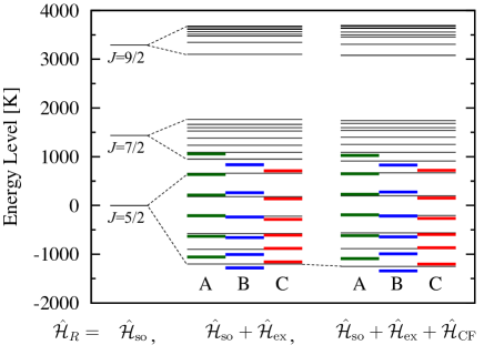
Figure 3: (color online) Calculated energy levels of the Sm-$4f$ states in SmFe₁₂ at ${\bm{B}}={\bm{0}}$. Analytical results $E^{X}_{M}$ with $X$=A, B, and C for corresponding model approximations in Eq. (43) are given by thick green (A), blue (B) and red lines (C), respectively. To clarify the contributions from $\hat{\cal{\cal H}}_{\rm so},\hat{\cal H}_{\rm ex},$ and $\hat{\cal H}_{\rm CF}$, we take original Hamiltonian $\hat{\cal H}_{R}$ as $\hat{\cal H}_{R}=\hat{\cal H}_{\rm so}$, $\hat{\cal H}_{\rm so}+\hat{\cal H}_{\rm ex}$, and $\hat{\cal H}_{\rm so}+\hat{\cal H}_{\rm ex}+\hat{\cal H}_{\rm CF}$. The numerically exact results are also shown by thin black lines.

Fig. 3 shows the diagonal matrix element $E_{M}^{X}$ ($X$=A, B, and C) of the effective lowest-$J$ multiplet Hamiltonian $\hat{\cal H}_{R}^{{\rm eff}J}$ at $T=0$ in Eq. (43). Note that CF coefficients and exchange fields are determined by the first principles, and the same values are used for models A, B and C. The results are compared with the exact results. To distinguish the contribution from each $\hat{\cal H}_{\rm so},$ $\hat{\cal H}_{\rm ex}$, and $\hat{\cal H}_{\rm CF}$ in $\hat{\cal H}_{R}$ of Eq. (6), the original Hamiltonian $\hat{\cal H}_{R}$ is taken as $\hat{\cal H}_{\rm so}$, $\hat{\cal H}_{\rm so}+\hat{\cal H}_{\rm ex}$, or $\hat{\cal H}_{\rm so}+\hat{\cal H}_{\rm ex}+\hat{\cal H}_{\rm CF}$.

Let us first describe the characteristics for the result $\hat{\cal H}_{R}=\hat{\cal H}_{\rm so}+\hat{\cal H}_{\rm ex}$. In model A, the sixfold degeneracy of energy levels given by $\hat{\cal H}_{\rm so}$ splits into equi-energy levels as $E_{M}^{\rm A}=E_{J}+\Delta_{\rm ex}(0)M$. In model B, the equi-energy levels shift to lower energy states by $J$-mixing term, $E_{M}^{\rm B}=E_{J}+\Delta_{\rm ex}(0)M-|\langle J,M|\hat{\cal H}_{\rm ex}|J+1,M\rangle^{2}/\Delta_{\rm so}.$ In model C, the energy shifts, which was over-estimate by the $J$-mixing term, are corrected.

The results obtained by $\hat{\cal H}_{R}=\hat{\cal H}_{\rm so}+\hat{\cal H}_{\rm ex}+\hat{\cal H}_{\rm CF}$ show that the effect of CF potentials on the energy levels is weak, as expected, and they reproduce the results obtained by the numerical exact diagonalization method as shown in Fig. 3.

III.2.3 Finite Temperature Perturbation for Single $R$ Ion

We apply the first-order perturbation at finite temperature assuming $\hat{\cal H}_{\rm ex}^{J}\gg\hat{\cal H}_{\rm CF}^{J}+\hat{\cal H}_{\rm Z}^{J}+\hat{\cal H}_{\rm mix}^{X}$. The unperturbed and perturbed Hamiltonians are $\hat{\cal H}_{\rm ex}^{J}=\Delta_{\rm ex}(T)C_{0}^{(1)}(\hat{\bm{J}})\equiv\hat{\cal H}^{(0)}$ and $\hat{\cal H}_{\rm CF}^{J}+\hat{\cal H}_{\rm Z}^{J}+\hat{\cal H}_{\rm mix}\equiv\hat{\cal H}^{\prime}$, respectively. Note that $\hat{\cal H}_{\rm so}$ is effectively taken into account in the $J$-multiplet formation of the $R$ ion. The approximated Gibbs free energy for $R$-$4f$ partial system on $j$-th $R$ site up to first-order perturbation is formally expressed as $g_{j}({\bm{e}}^{TM},T,{\bm{B}})=-k_{\rm B}\ln Z_{0}(T)+\sum_{M}\rho_{M}^{(0)}(T)\langle J,M|\hat{\cal H}^{\prime}|J,M\rangle$, where $E_{M}^{(0)}(T)=\Delta_{\rm ex}(T)M$, $Z_{0}(T)=\sum_{M}\exp[-\beta E_{M}^{(0)}(T)]$, and $\rho_{M}^{(0)}(T)=\exp[-\beta E_{M}^{(0)}(T)]/Z_{0}(T)$. More explicitly, it is given as,

$$g({\bm{e}}^{TM},T,{\bm{B}})= k_{\rm B}T\sum_{M}\rho_{M}^{(0)}(T)\ln\rho_{M}^{(0)}(T)$$

$$+\sum_{M}\rho_{M}^{(0)}(T)E_{M},$$ (44)

by using $E_{M}$ in Eq. (43). It is noted that $g({\bm{e}}^{TM},T,{\bm{B}})$ is model dependent because $E_{M}$ equals to $E_{M}^{\rm A}$, $E_{M}^{\rm B}$ or $E_{M}^{\rm C}$, corresponding to the model adopted.

By using Helmholtz free energy $f({\bm{e}}^{TM},T)$ for $R$-$4f$ partial system, the Gibbs free energy in the modified effective lowest-$J$ model is given as,

$$g({\bm{e}}^{TM},T,{\bm{B}})= f({\bm{e}}^{TM},T)-m(T){\bm{e}}^{TM}\cdot{\bm{B}},$$ (45)

$$m(T)= \mu_{\rm B}\left[g_{J}JB_{J}^{1}(x)-\frac{2(L+1)}{3(J+1)}T_{J}^{1}(x)\right],$$ (46)

with

$$f({\bm{e}}^{TM},T)= k_{\rm B}T\sum_{M}\rho_{M}^{(0)}(T)\ln\rho_{M}^{(0)}(T)$$

$$+f_{\rm ex}(T)+f_{\rm CF}({\bm{e}}^{TM},T),$$ (47)

$$f_{\rm ex}(T)= -\Delta_{\rm ex}(T)\left[JB_{J}^{1}(x)+\frac{L+1}{3S}T_{J}^{1}(x)\right],$$ (48)

$$f_{\rm CF}({\bm{e}}^{TM},T)= \sum_{l,m}A_{l}^{m}\langle r^{l}\rangle\Xi_{l}^{J}\frac{t_{l}^{m}({\bm{e}}^{TM})}{a_{l,m}}$$

$$\times\left[J^{l}B_{J}^{l}(x)+\frac{l(l+1)}{2l+1}T_{J}^{l}(x)\right].$$ (49)

Here $x\equiv J\Delta_{\rm ex}(T)/k_{\rm B}T$, and the model dependence appears in $T_{J}^{l}(x)$, which is denoted as $T_{J}^{l,X}(x)$ with $X$=A, B or C. For $X$=A, $T_{J}^{l,\rm{A}}(x)=0$ and for $X$=B and C,

$$T_{J}^{l,{\rm B(C)}}(x)= \frac{\Delta_{\rm ex}(T)}{\Delta_{\rm so}}\left[\frac{2J+l+1}{2}V_{J}^{l-1,{\rm B(C)}}(x)\right.$$

$$\qquad\qquad\left.-\frac{2}{2J+l+2}V_{J}^{l+1,{\rm B(C)}}(x)\right],$$ (50)

with

$$V_{J}^{l,{\rm B}}(x)= J^{l}B_{J}^{l}(x),$$ (51)

$$V_{J}^{l,{\rm C}}(x)= J^{l}B_{J}^{l}(x)-\frac{\Delta_{\rm ex}(T)}{\Delta_{\rm so}}\frac{L+S+1}{S(J+2)}$$

$$\times\left[\frac{l(2J-l+1)(2J+l+1)}{4(2l+1)}J^{l-1}B_{J}^{l-1}(x)\right.$$

$$\qquad\left.+\frac{l+1}{2l+1}J^{l+1}B_{J}^{l+1}(x)\right],$$ (52)

where $B_{J}^{l}(x)$ is the generalized Brillouin function Kuzminlinear defined by $(-1)^{l}J^{l}B_{J}^{l}(x)=\langle C_{0}^{(l)}(\hat{\bm{J}})\rangle_{0}$ with $x=J\Delta_{\rm ex}(T)/k_{\rm B}T$ for $l\geq 0$, where $\langle\hat{\bm{A}}\rangle_{0}=\sum_{M}\rho_{M}^{(0)}(T)\langle J,M|\hat{\bm{A}}|J,M\rangle$. The analytical expression of $B_{J}^{l}(x)$ is given in Ref. Magnani and $T_{J}^{l,\rm A}(x)=0$, $T_{J}^{l,\rm B}(x)$ and $T_{J}^{l,\rm C}(x)$ are linear combination of $B_{J}^{l-1}(x)$ and $B_{J}^{l+1}(x)$, and $B_{J}^{l-2}(x)$, $B_{J}^{l}(x)$, and $B_{J}^{l+2}(x)$, respectively, as shown in Eq. (50).

Because of the first-order perturbation for $\hat{\cal H}_{\rm Z}^{\prime}$, an analytical expression of the magnetic moment $m(T)$ is obtained as $m(T)=m_{L}(T)+m_{S}(T)$ with:

$$m_{L}(T) =\mu_{\rm B}\left[\frac{L+1}{J+1}JB_{J}^{1}(x)+\frac{2(L+1)}{3(J+1)}T_{J}^{1}(x)\right],$$ (53)

$$m_{S}(T) =-2\mu_{\rm B}\left[\frac{S}{J+1}JB_{J}^{1}(x)+\frac{2(L+1)}{3(J+1)}T_{J}^{1}(x)\right],$$ (54)

where $m_{L}(T)$ and $m_{S}(T)$ are orbital and spin component of magnetic moment on the $R$ ion. It is noted that $m_{L}(T)$ and $m_{S}(T)$ are model dependent because of the model dependence of $T_{J}^{l}(x)$ as shown above.

Within the finite temperature perturbation theory, the angular ${\bm{e}}^{TM}$ dependent part of single $R$ ion free energy $f({\bm{e}}^{TM},T)$ in Eq. (47) with the tetragonal symmetry can be written by:

$$f({\bm{e}}^{TM},T)= k_{1}(T)\sin^{2}\theta$$

$$+\left[k_{2}(T)+k_{2}^{1}(T)\cos 4\varphi^{TM}\right]\sin^{4}\theta^{TM}$$

$$+\left[k_{3}(T)+k_{3}^{1}(T)\cos 4\varphi^{TM}\right]\sin^{6}\theta^{TM}$$

$$+C(T),$$ (55)

which is a truncated form of $g({\bf e}^{TM},T,{\bm{0}})$ in Eq. (18). The $C(T)$ is an angle independent constant. For example, the leading anisotropy constants for a trivalent magnetic light $R$ ion (Ce³⁺, Pr³⁺, Nd³⁺, Pm³⁺, and Sm³⁺) can be written as follows:

$$k_{1}(T) =-3\left[J^{2}B_{J}^{2}(x)+\frac{6}{5}T_{J}^{2}(x)\right]A_{2}^{0}\langle r^{2}\rangle\Xi_{2}^{J}$$

$$-40\left[J^{4}B_{J}^{4}(x)+\frac{20}{9}T_{J}^{4}(x)\right]A_{4}^{0}\langle r^{4}\rangle\Xi_{4}^{J}$$

$$-168\left[J^{6}B_{J}^{6}(x)+\frac{42}{13}T_{J}^{6}(x)\right]A_{6}^{0}\langle r^{6}\rangle\Xi_{6}^{J},$$ (56)

$$k_{2}(T) =35\left[J^{4}B_{J}^{4}(x)+\frac{20}{9}T_{J}^{4}(x)\right]A_{4}^{0}\langle r^{4}\rangle\Xi_{4}^{J}$$

$$+378\left[J^{6}B_{J}^{6}(x)+\frac{42}{13}T_{J}^{6}(x)\right]A_{6}^{0}\langle r^{6}\rangle\Xi_{6}^{J}.$$ (57)

All terms of MA constants $k^{(q)}_{p}(T)$ in model A,B, and C are given by linear terms with respect to $A_{l}^{m}\langle r^{l}\rangle$.

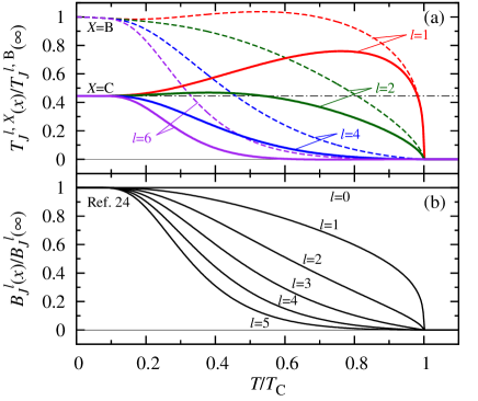
Figure 4: (color online) Temperature dependence of (a) $T_{J}^{l,\rm B(C)}(x)$ scaled by $T_{J}^{l,{\rm B}}(\infty)>0$ in Eq. (50) for model B(C) with broken(solid) curves and (b) generalized Brillouin function $B_{J}^{l}(x)/B_{J}^{l}(\infty)$ Kuzminlinear with $J=5/2$ and $x=J\Delta_{\rm ex}(T)/k_{\rm B}$, where the temperature is scaled by Curie temperature $T_{\rm C}$. The dashed-dotted line represent the value of $R_{J}$ (see text).

We may rewrite the approximations used and adopted in the present formalism by using $T_{J}^{l,X}(x)$ in Eq. (50) as follows:

• model A: Lowest-$J$ multiplet without mixing as $\Delta_{\rm ex}(T)/\Delta_{\rm so}=0$ or $T_{J}^{l,{\rm A}}(x)=0$ Kuzminlinear

• model B: Effective lowest-$J$ multiplet with mixing as $\left[\Delta_{\rm ex}(T)/\Delta_{\rm so}\right]^{2}=0$ or $T_{J}^{l,{\rm B}}(x)$ Kuzminmix ; Magnani

• model C: Modified effective lowest-$J$ multiplet with mixing as $T_{J}^{l,{\rm C}}(x)$ (present study).

At $T=0$, we have found a following simple relation holds between $T_{J}^{l,{\rm C}}(\infty)$ and $T_{J}^{l,{\rm B}}(\infty)$ as:

$$R_{J}=\displaystyle\frac{T_{J}^{l,{\rm C}}(\infty)}{T_{J}^{l,{\rm B}}(\infty)}=1-\frac{\Delta_{\rm ex}(0)}{\Delta_{\rm so}}\frac{(L+S+1)J}{S(J+2)}.$$ (58)

Because $R_{J}$ is independent of $l$, relations among the models $X$=A, B, and C on $m_{L,S}^{X}(0)$ and $k_{p}^{(q,)X}(0)$ can be generally expressed as follows:

$$m_{L,S}^{\rm C}(0) =m_{L,S}^{\rm A}(0)+R_{J}\left[m_{L,S}^{\rm B}(0)-m_{L,S}^{\rm A}(0)\right],$$ (59)

$$k_{p}^{(q,)\rm C}(0) =k_{p}^{(q,)\rm A}(0)+R_{J}\left[k_{p}^{(q,)\rm B}(0)-k_{p}^{(q,)\rm A}(0)\right].$$ (60)

At finite temperatures, $T_{J}^{l,{\rm B(C)}}(x)$ for $J=5/2$ scaled by $T_{J}^{l,{\rm B}}(\infty)>0$ are shown in Fig. 4(a) for the SmFe₁₂ compound. Here, $\Delta_{\rm ex}(T)/\Delta_{\rm so}$ is taken to be $0.206\alpha(T)$. For comparison purpose, we also show the $B_{J}^{l}(x)/B_{J}^{l}(\infty)$ in Fig. 4(b). $B_{J}^{l}(x)$ decays faster than $T_{J}^{l,{\rm B(C)}}(x)$ with increasing temperature. Thus the $J$-mixing effects included in $T_{J}^{l,{\rm B(C)}}(x)$ remain even at high temperatures.

III.2.4 Thermodynamic Analysis

Finally we investigate the thermodynamical instability by using the thermodynamic relation between Gibbs and Helmholtz free energy, which explicitly contains the CF potentials and the exchange field determined by first principles. We have to note that above the room temperature the exchange contribution $\hat{\cal H}_{\rm ex}$ decreases with increasing temperature at a rate proportional to $\alpha(T)$, so the energy hierarchy is changed and thermal fluctuation effects have to be considered as $k_{\rm B}T\gg\hat{\cal H}_{\rm CF}\sim\hat{\cal H}_{\rm ex}$. Even in this case, the formulation derived here based on generalized Brillouin function holds as shown by Kuz’min in Refs. Kuzminmix ; Kuzminlimit . In this thermodynamic analysis, we use the model C.

By applying the finite temperature perturbation theory to the lowest-$J$ multiplet Hamiltonian, the approximated Gibbs free energy density for whole system can be expressed as:

$$G({\bm{e}}^{TM},T,{\bm{B}}) =F({\bm{e}}^{TM},T)-{\bm{M}}_{\rm s}(T)\cdot{\bm{B}},$$ (61)

$$F({\bm{e}}^{TM},T) =\frac{1}{V_{0}}\sum_{j=1}^{n_{R}}f_{j}({\bm{e}}^{TM},T)+K_{1}^{TM}(T)\sin^{2}\theta^{TM},$$ (62)

$${\bm{M}}_{\rm s}(T) =\left[\frac{1}{V_{0}}\sum_{j=1}^{n_{R}}{m}_{j}(T)+M^{TM}(T)\right]{\bm{e}}^{TM},$$ (63)

where $F({\bm{e}}^{TM},T)$ is Helmholtz free energy density for whole system with model C and $f_{j}({\bm{e}}^{TM},T)$ and $m_{j}(T){\bm{e}}^{TM}$ are corresponding energy for $4f$-shell and expectation value of magnetic moment on $j$-th $R$ ion given in Eq. (47) and Eq. (46), respectively. The temperature dependence of $G({\bm{e}}^{TM},T,{\bm{B}})$ can be expressed as the linear combination of the generalized Brillouin functions for $R$ ion $B_{J}^{l}(J\Delta_{\rm ex}/k_{\rm B}T)$ and the temperature coefficient for $TM$ ion $\alpha(T)$ in Eq. (12). The equilibrium condition is the same as Eq. (17), where ${\bm{e}}_{0}^{TM}$ becomes the direction of total magnetization in the equilibrium. We can also analyze the instability of magnetic metastable states, which are crucially important in permanent magnetic materials. The metastable condition is $\delta G(T,{\bm{e}}^{TM},{\bm{B}})>0$ for given $T$ and ${\bm{B}}$ with $|e^{TM}|=1$.

The MA constants in whole system are obtained by combining the contribution from $R$ sublattice in Eq. (55) with Fe sublattice same as Eqs. (21) and (22). $K_{1}(T)$ can be substituted into the so called Krönmuller equation Kronmuller1 ; Kronmuller-text to obtain the coercive field

$$B_{\rm c}(T) =\alpha B_{\rm N}(T)-N_{\rm eff}M_{\rm s}(T),$$ (64)

$$B_{\rm N}(T) =\frac{2K_{1}(T)}{M_{\rm s}(T)},$$ (65)

where $B_{\rm c}(T)$ and $B_{\rm N}(T)$ are coercive and nucleation field, respectively. $\alpha(<1)$ is microstructural parameter and $N_{\rm eff}$ is local effective demagnetization factor Kronmuller-text . The $B_{\rm N}(T)$ gives upper limit of $B_{\rm c}(T)$.

IV Calculated Results for SmFe₁₂

IV.1 Valence Mechanism of Magnetic Anisotropy

We first calculate the charge density distribution and Coulomb potential at 0 K on constituent atoms of SmFe₁₂ lattice (Fig. 1) using the first principles. The calculated results determine the values of CF acting on $4f$ electrons, the magnitude of the exchange field $B_{\rm ex}(0)$ acting on the $J$, and the magnitude of $TM$ sublattice magnetization. These values are used for parameter values in the model Hamiltonian. The contribution to the CF from the charge density distribution inside (outside) the muffin-tine sphere radius is called ”valence (lattice) contribution” Hummler0 . If the CF is dominated by the former contribution, we call the mechanism of the MA ”valence mechanism” Tsuchiura1 .

The charge density distributions of single $R$ ion are approximately replaced with charge density on atomic orbitals of $6p$ and $5d$ states. To evaluated the valence contribution to CF parameters $A_{l}^{0}\langle r^{l}\rangle(val)$, we introduce distribution parameters $\Delta n_{6p}^{(2)},\Delta n_{5d}^{(2)}$ Coehoorn ; Sakuma and $\Delta n_{5d}^{(4)}$ defined as,

$$\Delta n_{n^{\prime}l^{\prime}}^{(l)}=\frac{4\pi}{2l+1}a_{l,0}\sum_{m^{\prime}}\int d\Omega\ t_{l}^{0}(\theta,\varphi)|t_{l^{\prime}}^{m^{\prime}}(\theta,\varphi)|^{2}n_{n^{\prime}l^{\prime},m^{\prime}},$$ (66)

where $\Omega$ is the solid angle and $m^{\prime}$ indicates the multiple orbitals for the quantum number ($n^{\prime}l^{\prime}$). The shape of the function $t_{l}^{0}(\theta,\varphi)$ in Eq. (66) is given in Fig. 5(c).

The particular cases are as follows:

$$\Delta n_{6p}^{(2)}= \frac{1}{5}\left[n_{6p,z}-\frac{1}{2}(n_{6p,x}+n_{6p,y})\right],$$ (67)

$$\Delta n_{5d}^{(2)}= \frac{1}{7}\left[n_{5d,z^{2}}+\frac{1}{2}(n_{5d,xz}+n_{5d,yz})\right.$$

$$\quad\left.\vphantom{\frac{1}{7}}-(n_{5d,x^{2}-y^{2}}+n_{5d,xy})\right],$$ (68)

$$\Delta n_{5d}^{(4)}= \frac{1}{28}\left[n_{5d,z^{2}}-\frac{2}{3}(n_{5d,xz}+n_{5d,yz})\right.$$

$$\qquad\left.+\frac{1}{6}(n_{5d,x^{2}-y^{2}}+n_{5d,xy})\right],$$ (69)

where $n_{n^{\prime}l^{\prime},m^{\prime}}$ is the occupation number of the ($n^{\prime}l^{\prime}$, $m^{\prime}$) orbital. We note that $\Delta n_{6p}^{(4)}=0$. Valence contribution of $A_{2}^{0}\langle r^{2}\rangle$ and $A_{4}^{0}\langle r^{4}\rangle$ are determined as Richter1 ; Hummler0 ,

$$A_{2}^{0}\langle r^{2}\rangle(val) =F^{(2)}(4f,6p)\Delta n_{6p}^{(2)}+F^{(2)}(4f,5d)\Delta n_{5d}^{(2)},$$ (70)

$$A_{4}^{0}\langle r^{4}\rangle(val) =F^{(4)}(4f,5d)\Delta n_{5d}^{(4)},$$ (71)

with the Slater-Condon parameters:

$$F {}^{(l)}(4f,n^{\prime}l^{\prime})$$

$$=\frac{e^{2}}{4\pi\varepsilon_{0}}\iint_{0}^{r_{c}}\frac{r_{<}^{l}}{r_{>}^{l+1}}r^{2}|R_{4f}(r)|^{2}r^{\prime 2}|R_{n^{\prime}l^{\prime}}(r^{\prime})|^{2}dr^{\prime}dr>0,$$ (72)

where $r_{<}=\min(r,r^{\prime})$ and $r_{>}=\max(r,r^{\prime})$. Via Eqs. (70) and (71), the distribution parameters $\Delta n_{n^{\prime}l^{\prime}}^{(l)}$ determine $A_{l}^{0}\langle r^{l}\rangle(val)$. It may be noted that no $6p$ and $5d$ orbitals exist for $A_{6}^{0}\langle r^{6}\rangle(val)$.

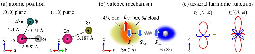
Figure 5: (color online) (a) Atomic position of first ($8i$), second ($8j$), and third ($8f$) neighbor Fe atoms of Sm ion in SmFe₁₂, (b) illustration of valence mechanism Tsuchiura1 in SmFe₁₂, and (c) typical tesseral harmonic functions as basis of CF Hamiltonian, where signs represent the phase.

A simple explanation for the appearance of the uniaxial MA in a Sm ion surrounded by Fe atoms is given as follows. Fig. 5(a) shows the lattice strucutre of SmFe₁₂ Hirayama2 ; Harashima . Left panel of Fig. 5(b) shows the location of Sm and Fe on (010) plane of the lattice. Because of the short atomic distance between Sm and the first nearest neighbor (n.n.) Fe($8i$) sites, the distribution of valence electrons on Sm extends within the $a-b$ plane as shown in Fig. 5(c). According to the negative sign of $t_{2}^{0}(\theta,\varphi)$ in Fig. 5(d), the distribution parameters defined by Eq. (66) in terms of electron numbers of $6p$ and $5d$-orbitals are negative; $\Delta n_{6p}^{(2)}=-0.0012$, $\Delta n_{5d}^{(2)}=-0.0011$. Therefore, we obtain $A_{2}^{0}\langle r^{2}\rangle(val)<0$ by Eq. (70) in agreement with the numerical value of $A_{2}^{0}\langle r^{2}\rangle$ shown in TABLE 1. As shown by Eq. (56) the main contribution of the MA constant $k_{1}(T)$ is given by a product of $A_{2}^{0}$ and the positive value of Stevens factor $\Theta_{2}^{0}$, and $k_{1}(T)$ becomes positive. This means that the $K_{1}(T)>0$ because $K_{1}^{TM}(T)>0$.

On the other hand, second neighbor Fe(8$j$) and third neighbor Fe(8$f$) atoms of Sm atom are situated obliquely upward as shown in Fig. 5(b). According to the negative sign of $t_{4}^{0}(\theta,\varphi)$ shown in Fig. 5(d), we obtained $\Delta n_{5d}^{(4)}=-0.0013$ using Eq. (69), and $A_{4}^{0}\langle r^{4}\rangle(val)<0$ from Eq. (71). Again the negative value is consistent with the numerical values of $A_{4}^{0}\langle r^{4}\rangle$. The main contribution of MA constant $k_{2}(T)$ comes from a product of $A_{4}^{0}\langle r^{4}\rangle$ and the positive value of $\Theta_{4}^{0}$, and results in $K_{2}(T)<0$.

Thus, the sign of MA constants $K_{1}(T)$ and $K_{2}(T)$ are determined by the configuration of Sm and Fe atoms in the lattice. In the following, we investigate the $J$-mixing effect on single Sm magnetic properties at $T=0$ K.

IV.2 $J$-Mixing Effect and Zero-Temperature Magnetic Properties of SmFe₁₂ Compound

To clarify the $J$-mixing effect on single-ion magnetic properties, we show the calculated results of the magnetic moments $m_{L,S}(0)$ and the MA constants $k_{1,2}(0)$ for model A, B, and C in TABLE 3. We used Eqs. (53) and (54) for $m_{L,S}(0)$ and Eqs. (56) and (57) for $k_{1,2}(0)$, and the values of $A_{l}^{m}\langle r^{l}\rangle$, $B_{\rm ex}(0)$, and $M^{TM}(0)$ in TABLE 1. As a reference, we also show the results obtained by the statistical method: $m_{L,S}(0,{\bm{0}})$ in Eqs. (23) and (24) and $k_{1,2}(0)$ defined in Eqs. (19) and (20). Both the analytical and statistical results give $k_{1}(0)>0$ and $k_{2}(0)<0$ for three models A, B, and C. The calculated results in model C (present model) agree best with the statistical ones.

We find that the absolute values of $m_{L,S}(0)$ and $k_{1,2}(0)$ in model B and C are larger than those in model A, which is attributed to inclusion of the $J$-mixing effects. The model B proposed in the previous studies Kuzminmix ; Magnani over-estimated the $J$-mixing effects by $1/R_{J}$ compared with model C, where $R_{J}=0.44$ in Eq. (58) for SmFe₁₂ compound. Actually, values of $m_{L,S}^{\rm C}$ and $k_{1,2}^{\rm C}$ in TABLE 3 satisfy the relation in Eq. (59) and (60). The results in present study ($X$=C) quantitatively agree well with statistical ones except for $k^{\rm C}_{2}(0)$. The discrepancy in $k^{\rm C}_{2}(0)$ may be due to omitting the 2nd order terms of $A_{2}^{0}\langle r^{2}\rangle$ in Eq. (57), which have a positive contribution independent of the sign of $A_{2}^{0}\langle r^{2}\rangle$ Kuzmin2nd .

Table 3: Magnetic moments $m_{L,S}(0)$ [$\mu_{\rm B}$] in Eqs. (53) and (54) and MA constants $k_{1,2}(0)$ [K] in Eqs. (56) and (57) for model A, B, and C at 0 K for single Sm ion. Results obtained by Boltzamann statistics of $m_{L,S}(0,{\bm{0}})$ defined by Eqs. (23) and (24) and $k_{1,2}(0)$ defined by Eqs. (19) and (20) are also shown in the fifth column.

model	A	B	C	statistics
$m_{L}$	4.29	5.04	4.62	4.70
$m_{S}$	-3.57	-5.08	-4.24	-4.39
$k_{1}$	60.2	144.5	97.7	101.1
$k_{2}$	-14.0	-74.6	-40.9	-23.5

IV.3 Finite Temperature Magnetic Properties
of SmFe₁₂ Compound

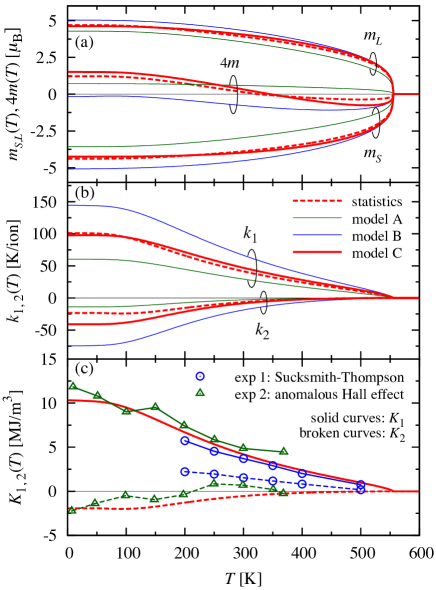
Figure 6: (color online) Temperature dependence of (a) magnetic moments of Sm ion $m_{L,S}(T)$ and $m(T)$ at ${\bm{B}}={\bm{0}}$ and (b) MA constants per single Sm ion $k_{1,2}(T)$ calculated by using models A, B and C. Results obtained by Boltzmann statistics are shown by broken curves. (c) Temperature dependent MA constants $K_{1,2}(T)$ in SmFe₁₂ compound by using statistical method for Sm sublattice contribution $k_{1,2}(T)$, which are compared with experimental ones by the Sucksmith-Thompson (circles) Hirayama2 and the anomalous Hall effect (triangles) Ogawa2 . For both calculated and experimental results in Fig. (c), $K_{1}(T)$ and $K_{2}(T)$ are shown by solid and broken curves, respectively.

Calculated results of finite temperature magnetic properties for a single Sm ion in equilibrium at ${\bm{e}}^{TM}_{0}={\bm{n}}_{c}$: the magnetic moment $m_{L,S}(T)$ in Eqs. (53) and (54) and the MA constants $k_{1,2}(T)$ in Eqs. (56) and (57) are shown in Fig. 6(a) and (b), respectively. The results show that the $J$-mixing effect in model B increases the absolute values of both $m_{L,S}(T)$ and $k_{1,2}(T)$. The over-estimation in model B is modified by the present model C in the whole temperature range. Obtained results of model C reproduce well the statistical results for $m_{L,S}(T,{\bm{0}})$ in Eqs. (23) and (24) and for $k_{1,2}(T)$ in Eqs. (19) and (20) as shown by broken lines in Fig. 6(a) and (b).

The physical meaning of the increment of the absolute value of $m_{L,S}(T)$ and $k_{1,2}(T)$ by $J$-mixing may be given as follows. The expression of the free energy given by Eq. (48) includes the $J$-mixing effect in the second term of the square bracket. The term decrease $f_{\rm ex}(x)$ by $-\mu_{\rm B}B_{\rm ex}(T)\delta S(T)$, where $\displaystyle\delta S(T)=\frac{2(L+1)}{3(J+1)}T_{J}^{1}(T)>0$. Because of the decrease in $f_{\rm ex}(x)$, the absolute value of the spin $\langle C^{(1)}_{0}(\hat{\bm{S}})\rangle_{0}$ and orbital moments $\langle C^{(1)}_{0}(\hat{\bm{L}})\rangle_{0}$ along ${\bm{e}}_{0}^{TM}$ are increased by $\delta S(T)$. The tensor operators $\langle C^{(l)}_{0}(\hat{\bm{L}})\rangle_{0}$ for even $l$ are also increased by $\displaystyle\frac{l(l+1)}{2l+1}T_{J}^{l}(x)$, which contribute to increase in the absolute value of the MA constants $k_{p}^{(q)}(T)$.

The magnetic moment of Sm ion $m(T)$ is reversed at around $T_{\rm comp}=350$ K in model C and calculation by Boltzmann statistics. The temperature is called compensation temperature. This phenomenon is observed also in other Sm compounds Adachi1 ; Adachi2 . Zhao $et$ $al$ pointed out that this phenomenon also appears at $T=337$ K in Sm₂Fe₁₇N_x using statistical method including similar parameter values with ours such as $\mu_{B}B_{\rm ex}(0)/k_{\rm B}=300$ K and $\lambda/k_{\rm B}=411$ K Zhao . Their results are comparable with ours, however, the mechanism has not been surveyed. In the present model C, the magnetic moment of Sm ion can be written as $m(T)=g_{J}\mu_{\rm B}JB_{J}^{1}(x)-\mu_{\rm B}\delta S(T)$. Because $\mu_{\rm B}\delta S(T)$ is proportional to $T_{J}^{1,{\rm C}}(x)$ and monotonically increasing with temperature below $T/T_{\rm C}=0.8$ as shown in Fig. 4(a), the term compensates the $g_{J}\mu_{\rm B}JB_{J}^{1}(x)$ at $T_{\rm comp}$.

Fig. 6(c) shows the results of $K_{1}(T)$ and $K_{2}(T)$ obtained by statistical method in SmFe₁₂ compound, which are compared with experimental ones denoted by exp 1 and exp 2 measured by the Sucksmith-Thompson method Hirayama2 and anomalous Hall effect Ogawa2 , respectively. At the whole temperature region the results of $K_{1}(T)$ agree well with the experiments. Our statistical results qualitatively reproduce the experimental results below 200 K. The negative $K_{2}(T)$ at low temperatures is origin of first-order magnetization process (FOMP) as discussed below.

IV.4 Thermodynamic Properties
of SmFe₁₂ Compound

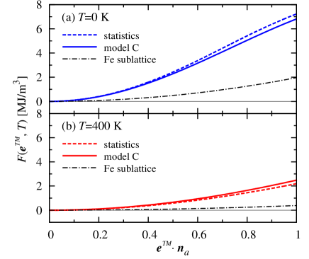
Figure 7: (color online) Dependence of Helmholtz free energy density on ${\bm{e}}^{TM}\cdot{\bm{n}}_{a}$ with ${\bm{e}}^{TM}\cdot{\bm{n}}_{b}=0$ in SmFe₁₂ at (a) $T=0$ and (b) 400 K. Analytical results $F({\bm{e}}^{TM},T)$ in Eq. (62) and results of $G({\bm{e}}^{TM},T,{\bm{0}})$ obtained by Boltzmann statistics in Eq. (14) are shown by solid and broken curves, respectively, in which the contribution from Fe sublattice is included. The dashed-dotted curves represent the Fe sublattice MA energy: $K_{1}^{TM}(T)({\bm{e}}^{TM}\cdot{\bm{n}}_{a})^{2}$

Fig. 7 shows calculated results of the Helmholtz free energy density $F({\bm{e}}^{TM},T)$ given in Eq. (62) for model C as a function of ${\bm{e}}^{TM}\cdot{\bm{n}}_{a}$ with ${\bm{e}}^{TM}\cdot{\bm{n}}_{b}=0$ at $T=0$ K and $400$ K, where ${\bm{n}}_{a(b)}$ is unit vector parallel to $a(b)$-axis. The results are compared with statistical ones of $G({\bm{e}}^{TM},T,{\bm{0}})$ in Eq. (14). When the direction of ${\bm{e}}^{TM}$ is changed, the free energy density on both Sm and Fe sublattice are increased. For the Sm sublattice, the energy increase originates from the CF, which can be expressed by the $\sum_{j}f_{{\rm CF},j}({\bm{e}}^{TM},T)$ in Eq. (55), and for Fe sublattice, the energy increase can be written by: $K_{1}^{TM}(T)\sin^{2}\theta^{TM}$ with $K_{1}^{TM}(T)=1.966$ and $0.387$ MJ/m³ at 0 and 400 K, respectively, which are much smaller than those of Sm sublattice $\sum_{j}k_{1,j}(T)/V_{0}=8.059$ and $2.310$ MJ/m³. The analytical results agree well with statistical ones.

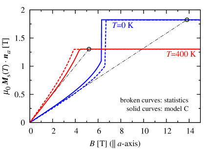
Figure 8: (color online) Magnetization curves of SmFe₁₂ at $T=0$ and 400 K with applied field $B$ parallel to $a$-axis in the equilibrium calculated by analytical (solid curves) and statistical (broken curves) methods in Eqs. (63) and (25), respectively, where $\mu_{0}$ is the magnetic constant. Dashed-dotted lines show tangent lines of magnetization curves at $B=0$: $y=[\mu_{0}M_{\rm s}(T)^{2}/2K_{1}]B$. Values of $B$ at the circles correspond to the nucleation field $B_{\rm N}(T)$ obtained by using the free energy density of model C (see text).

Fig. 8 shows calculated results of magnetization curves in the equilibrium states of SmFe₁₂ at $T=0$ and 400 K, where the magnetic field ${\bm{B}}$ is applied along $a$-axis. Analytical results of the magnetization along the $a$-axis are compared with statistical ones. We have confirmed that the results in model C well reproduce the statistical ones. At $T=0$, we find characteristic behavior of an abrupt change in the magnetization ${\bm{M}}_{\rm s}(T)\cdot{\bm{n}}_{a}$ at $B=B_{\rm FP}$. The change is called first-order magnetization process (FOMP) and the $B_{\rm FP}$ is called as FOMP field. At $T$=400 K, no FOMP appears in both analytical and statistical results and the magnetization saturates at the MA field $B_{\rm A}$. In SmFe₁₂, the magnetization curve at low temperatures were not reported, however, in SmFe₁₁Ti compound, FOMP observed at $T=5$ K and $B_{\rm FP}=10$ T Hu , which is qualitatively consistent with our results.

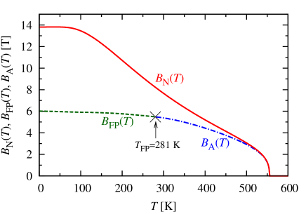
Figure 9: (color online) Temperature dependence of the nucleation field $B_{\rm N}(T)$, the MA field $B_{\rm A}(T)$, and the first-order magnetization process (FOMP) field $B_{\rm FP}(T)$ obtained by using the approximated free energy density of model C neglecting $K_{3}(T)$, $K_{2}^{1}(T)$, and $K_{3}^{1}(T)$, the details of which are shown in appendix A. $B_{\rm FP}(T)$ is the point of discontinuity in the FOMP realized below FOMP temperature $T_{\rm FP}$ (see text).

Let us consider the magnetization process along $c$-axis and estimate nucleation field $B_{\rm N}$ in the model C. The magnetization is first saturated as $M_{\rm s}(T){\bm{n}}_{c}$ along $c$-axis by an infinitesimal field. Then the direction of the magnetic field is reversed and the magnitude is increased as $-B{\bm{n}}_{c}$. The original state continues to exist as a quasi-stable state as far as the condition for a first-order variation $\delta G({\bm{n}}_{c},T,-B{\bm{n}}_{c})>0$ is satisfied. The magnetization tends to decline when $\delta G(nc,T,-B{\bm{n}}_{c})=0$. The applied magnetic field at which the latter condition is satisfied is the nucleation field, which has been given as $B_{\rm N}=2K_{1}(T)/M_{\rm s}(T)$ Kronmuller1 .

Because $B_{\rm N}$ corresponds to the field at which the magnetization begins to decline with infinitesimally angle $\theta$ against $c$-axis, the magnitude $B_{\rm N}$ in realistic system can be estimated once the magnetization curve is obtained along a hard axis. Fig. 8 shows the magnetization curve along $a$-axis calculated in the model C. $B_{\rm N}$ is given by a crossing point of the magnetization curve in the saturated state and the tangential line of the magnetization curve at zero field $y=\left[\mu_{0}M_{\rm s}(T)^{2}/2K_{1}(T)\right]$. When the value of $y=\mu_{0}M_{\rm s}$, the magnetic field coincides with $B_{\rm N}$ defined in Eq. (65).

The magnetization curves along hard and easy-axis in the case of $K_{1}(T)>0$ and $K_{2}(T)<0$ can be characterized by the nucleation field $B_{\rm N}(T)$, the FOMP field $B_{\rm FP}(T)$, and the MA field $B_{\rm A}(T)$. These values are analytically expressed by using the ratio $\gamma(T)=K_{1}(T)/K_{2}(T)$ as,

$$B_{\rm N}(T) =\frac{2K_{1}(T)}{M_{\rm s}(T)},$$ (73)

$$B_{\rm FP}(T) =B_{\rm N}[x_{\rm FP}(T)+2\gamma(T)x_{\rm FP}(T)^{3}]$$ (74)

$$\qquad\qquad\qquad\qquad(0<x_{\rm FP}(T)<1),$$

$$B_{\rm A}(T) =B_{\rm N}[1+2\gamma(T)]$$ (75)

$$\qquad\qquad\qquad\qquad(x_{\rm FP}(T)>1),$$

with

$$x_{\rm FP}(T) =\frac{1}{3}\left(-1+\sqrt{-\frac{3}{\gamma(T)}-2}\right),$$ (76)

where we use the approximate free energy density: $F({\bm{e}}^{TM},T)=K_{1}(T)\sin^{2}\theta^{TM}+K_{2}(T)\sin^{4}\theta^{TM}$, in which the small contributions $K_{3}(T)$, $K_{2,3}^{1}(T)$ are neglected. Details are shown in Appendix A. Calculated results of $B_{\rm N}(T)$, $B_{\rm FP}(T)$, and $B_{\rm A}(T)$ are shown in Fig. 9. The condition of FOMP appearance in model C is given by $-K_{2}(T)<K_{1}(T)<-6K_{2}(T)$ between $0<x_{\rm FP}(T)<1$ in Eq. (74). As for SmFe₁₂ compound, the FOMP is realized below $T=281$ K $\equiv$ $T_{\rm FP}$, which is analytically obtained from the condition: $K_{1}(T)=-6K_{2}(T)$. The curves of $B_{\rm FP}(T)$ and $B_{\rm A}(T)$ are continuously connected at $T_{\rm FP}$, which is called as FOMP temperature. When $K_{1}(T)<-K_{2}(T)$ the magnetization direction is in-plane at ${\bm{B}}={\bm{0}}$.

V Summary

The temperature dependence of magnetic anisotropy (MA) constants and magnetization of SmFe₁₂ were investigated by using two methods for the model Hamiltonian which combines quantum and phenomenological ones for rare-earth ($R$) and Fe subsystem, respectively. Parameter values of $R$ Hamiltonian were determined by the first-principles. First method adopts a numerical procedure with Boltzmann statistics for the Sm $4f$ electrons. The other one is an analytical method which deals with the magnetic states of $R$ ions with strong mixing of states with different quantum number of angular momentum $J$ ($J$-mixing). We have modified the previous analytical methods for Sm ions which have relatively small spin-orbit interaction, and clarified that they over-estimate the $J$-mixing effects for Sm-transition metal compounds. It has been shown that the results of our analytical method agree with those obtained by statistical method. Our analytical method revealed that the increasing spin angular momentum with $J$-mixing caused by strong exchange field, enhances the absolute value of orbital angular momentum and MA constants via spin-orbit interaction, and that these $J$-mixing effects remain even above room temperature. The calculated results of MA constants show that $K_{1}(T)>0$ and $K_{2}(T)<0$ in SmFe₁₂ in consistent with experiment.

The peculiar temperature dependence known as first-order magnetization process (FOMP) in SmFe₁₂ has been attributed to the negative $K_{2}$. It was also verified that the requirement for the appearance of FOMP is given as $-K_{2}<K_{1}<-6K_{2}$. The positive (negative) $K_{1(2)}$ appears due to an increase in the crystal field parameter $A_{2}^{0}\langle r^{2}\rangle$ ($A_{4}^{0}\langle r^{4}\rangle$) caused by hybridization between $3d$-electrons of Fe on $8i$ ($8j$) site and $5d$ and $6p$ valence electrons on Sm. The mechanism of $K_{1}>0$ and $K_{2}<0$ in SmFe₁₂ has been thus clarified by using the expressions of $K_{1}$ and $K_{2}$ obtained in the analytical method. Shortly, the sign of $K_{1}$ and $K_{2}$ in SmFe₁₂ is attributed to the characteristic lattice structure around Sm ions, that is, crystallographic 2$b$-sites on $c$-axis adjacent to Sm are vacant. We also present results on the magnetization process and nucleation fields by calculating Gibbs free energy.

The present method will be applied to derive a general expression of the free energy to analyze MA of non-uniform systems such as disordered compounds, surfaces, and interfaces. The results will be reported in a forthcoming paper.

Appendix A Magnetization Process in Condition
of $K_{1}(T)>0$ and $K_{2}(T)<0$

To investigate the magnetization process in equilibrium along the $c$-plane (e.g. $a$-axis), we introduce the simplified model with magnetic anisotropy constants $K_{1}(T)>0$ and $K_{2}(T)<0$, which can be expressed by the Gibbs free energy as:

$$G(x,T,B)=K_{1}(T)x^{2}+K_{2}(T)x^{4}- BM_{\rm s}(T)x$$ (77)

$$(|x|\leq 1),$$

where $x={\bm{M}}_{\rm s}(T)\cdot{\bm{n}}_{a}/M_{\rm s}(T)$ with total magnetization ${\bm{M}}_{\rm s}$ and unit vector parallel to $a$-axis ${\bm{n}}_{a}$. $T$ and ${\bm{B}}=B{\bm{n}}_{a}$ ($B>0$) are temperature and applied magnetic field, respectively. The equilibrium condition is:

$$G(x_{0},T,B)=\min_{|x|\leq 1}G(x,T,B),$$

where $x=x_{0}(T,B)$ gives minimum of $G(x,T,B)$. For $K_{1}(T)\leq-K_{2}(T)$, the magnetization is always tilted to the $a$-axis direction due to $x_{0}(T,B)=1$. Otherwise, the magnetization curve is given by:

$${\bm{M}}_{\rm s}(T,B)\cdot{\bm{n}}_{a}=M_{\rm s}(T)x_{0}(T,B).$$ (78)

The first-order magnetization process (FOMP) appears, when $x_{0}(T,B)$ has two values at certain $B$, which is called as FOMP field $B_{\rm FP}$.

To determine the $x_{0}(T,B)$ for $K_{1}(T)>-K_{2}(T)$, we show the first and second derivative of $G(x,T,B)$ with respect to $x$ as:

$$\frac{\partial G(x,T,B)}{\partial x} =2K_{1}(T)x+4K_{2}(T)x^{3}-BM_{\rm s}(T),$$ (79)

$$\frac{\partial^{2}G(x,T,B)}{\partial x^{2}} =2K_{1}(T)+12K_{2}(T)x^{2}.$$ (80)

A inflection point of $G(x,T,B)$ for $x>0$ at fixed $T$ and $B$ is given by $x_{c}(T)=\sqrt{-K_{1}(T)/6K_{2}(T)}$. Hereafter, we consider following two cases: $x_{c}(T)\geq 1$ and $x_{c}(T)<1$.

(i) The case of $x_{c}(T)\geq 1$

$x_{0}(T,B)$ is obtained from the condition $\partial G(x,T,B)/\partial x=0$ for $0<x\leq 1$, because $\partial^{2}G(x,T,B)/\partial x^{2}>0$ is always satisfied. The saturating point of magnetization $x_{0}(T,B)=1$ is obtained from the condition $\partial G(x,T,B)/\partial x|_{x=1}=0$ as:

$$B=\frac{2K_{1}(T)}{M_{\rm s}(T)}[1+2\gamma(T)]\equiv B_{\rm A}(T),$$ (81)

where $\gamma(T)=K_{2}(T)/K_{1}(T)$. The $B_{\rm A}$ is so-called anisotropy field.

(ii) The case of $x_{c}(T)<1$

$x_{0}(T,B)$ is obtained from the condition

$$G(x_{0},T,B)=\min\left[G(x_{e},T,B),G(1,T,B)\right],$$ (82)

where $x_{e}(T,B)$ is determined by the condition of local minium as: $\partial G(x,T,B)/\partial x=0$ and $x_{e}(T,B)<x_{c}(T)$. In the magnetization process, $x_{0}(T,B)$ is continuously increased from zero with increasing $B$ according to $x_{0}(T,B)=x_{e}(T,B)$ for $G(x_{e},T,B)<G(1,T,B)$. At $B=B_{\rm FP}$ such that $G(x_{e},T,B)=G(1,T,B)$ is satisfied, $x_{0}(T,B)$ shows the abrupt jump and becomes saturated value of $x_{e}(T,B)=1$. The condition is rewritten as:

$$(x_{0}-1)\left[3K_{2}(T)x_{0}^{2}+2K_{2}x_{0}+K_{1}(T)+K_{2}(T)\right]=0.$$ (83)

By solving the Eq. (83) for $0<x_{0}\leq 1$, two minimum points of $G(x,T,B)$ with respect to $x$ are obtained at $x_{0}(T,B)=1$ and

$$x_{0}(T,B)=\frac{1}{3}\left(-1+\sqrt{-\frac{3}{\gamma(T)}-2}\right)\equiv x_{\rm FP}(T).$$ (84)

By using $x_{\rm FP}(T)$, the field at which the FOMP occurs is determined by:

$$B=\frac{2K_{1}(T)}{M_{\rm s}(T)}[x_{\rm FP}(T)+2\gamma(T)x_{\rm FP}(T)^{3}]\equiv B_{\rm FP}(T).$$ (85)

As a result, for $-1<\gamma(T)<-1/6$, the FOMP occurs between ${\bm{M}}_{\rm s}(T)\cdot{\bm{n}}_{a}=M_{\rm s}(T)x_{\rm FP}(T)$ and $M_{\rm s}(T)$.

References

- (1) T. Miyake, K. Terakura, Y. Harashima, H. Kino, and S. Ishibashi, J. Phys. Soc. Jpn. 83, 043702 (2014).
- (2) Y. Hirayama, Y. K. Takahashi, S. Hirosawa, K. Hono, Scr. Mater. 95, 70 (2015).
- (3) G. C. Hadjipanayis, A. M. Gabay, A. M. Schönhöbel, A. Martín-Cid,J. M. Barandiaran, and D. Niarchos, Engineering 6, 141 (2020).
- (4) K. Ohashi, Y. Yokoyama, R. Osugi, Y. Tawara, IEEE Trans. Magn. MAG-23, 3101 (1987).
- (5) K. Ohashi, Y. Tawara, R. Osugi, and M. Shimao, J. Appl. Phys. 64, 5714 (1988).
- (6) Bo-Ping Hu, Hong-Shuo Li, J. P. Gavigan, and J. M. D. Coey, J. Phys.: Condens. Matter 1, 755 (1989).
- (7) T. Kuno, S. Suzuki, K. Urushibara, K. Kobayashi, N. Sakuma, M. Yano, A. Kato, and A. Manabe, AIP Advances 6, 025221 (2016).
- (8) A. M. Schönhöbel, R. Madugundo, O. Yu. Vekilova, O. Eriksson, H. C. Herper, J. M. Barandiarán, G. C. Hadjipanayis, J. Alloys Compd. 786, 969 (2019).
- (9) H. Kato, T. Nomura, M. Ishizone, H. Kubota, and T. Miyazaki, J. Appl. Phys. 87, 6125 (2000).
- (10) Y. Hirayama, Y. K. Takahashi, S. Hirosawa, and K. Hono, Scr. Mater. 138, 62 (2017).
- (11) D. Ogawa, X. D. Xu, Y. K. Takahashi, T. Ohkubo, S. Hirosawa, and K. Hono, Scr. Mater. 164, 140 (2019).
- (12) D. Ogawa, T. Yoshioka, X. D. Xu, Y. K. Takahashi, H. Tsuchiura, T. Ohkubo, S. Hirosawa, and K. Hono, J. Magn. Magn. Mater. 497, 165965 (2020).
- (13) H. Sepehri-Amin, Y. Tamazawa, M. Kambayashi, G. Saito, Y. K. Takahashi, D. Ogawa, T. Ohkubo, S. Hirosawa, M. Doi, T. Shima, and K. Hono, Acta Materialia 194, 337-342 (2020).
- (14) R. F. L. Evans, W. J. Fan, P. Chureemart, and T. A. Ostler, and M. O. A. Ellis, and R. W. Chantrell, J. Phys.: Condens. Matter 26, 103202 (2014).
- (15) Y. Toga, M. Matsumoto, S. Miyashita, H. Akai, S. Doi, T. Miyake, and A. Sakuma, Phys. Rev. B 94, 174433 (2016).
- (16) M. Nishino, Y. Toga, S. Miyashita, H. Akai, A. Sakuma, and S. Hirosawa, Phys. Rev. B 95, 094429 (2017).
- (17) T. Miyake and H. Akai J. Phys. Soc. Jpn. 87, 041009 (2018).
- (18) T. Yoshioka and H. Tsuchiura, Appl. Phys. Lett. 112, 162405 (2018).
- (19) H. Tsuchiura, T. Yoshioka, and P. Novák, Scr. Mater. 154, 248 (2018).
- (20) M. Yamada, H. Kato, H. Yamamoto, and Y. Nakagawa, Phys. Rev. B 38, 620 (1988).
- (21) R. Sasaki, D. Miura, and A. Sakuma, Appl. Phys. Express 8, 043004 (2015).
- (22) D. Miura, R. Sasaki, and A. Sakuma, Appl. Phys. Express 8, 113003 (2015).
- (23) D. Miura and A. Sakuma, AIP Advances 8, 075114 (2018).
- (24) M. D. Kuz’min, Phys. Rev. B 46, 8219 (1992).
- (25) M. D. Kuz’min and J. M. D. Coey, Phys. Rev. B 50, 12533 (1994).
- (26) M. D. Kuz’min, Phys. Rev. B 51, 8904 (1995).
- (27) Y. Millev and M. Fähnle, Phys. Rev. B 52, 4336 (1995).
- (28) M. D. Kuz’min, J. Appl. Phys. 92, 6693 (2002).
- (29) N. Magnani, S. Carretta, E. Liviotti, and G. Amoretti, Phys. Rev. B 67, 144411 (2003).
- (30) Y. Harashima, K. Terakura, H. Kino, S. Ishibashi, and T. Miyake, JPS Conf. Proc. 5, 011021 (2015).
- (31) W. Körner, G. Krugel, and C. Elsasser, Sci. Rep. 6, 24686 (2016).
- (32) P. Delange, S. Biermann, T. Miyake, and L. Pourovskii, Phys. Rev. B 96, 155132 (2017).
- (33) J. H. Van Vleck, The Theory of Electric and Magnetic Susceptibilities (Oxford University Press, Oxford, 1932).
- (34) S. G. Sankar, V. U. S. Rao, E. Segal, W. E. Wallace, W. G. D. Frederick, and H. J. Garrett, Phys. Rev. B 11, 435 (1975).
- (35) H. W. de Wijn, A. M. van Diepen, and K. H. J. Buschow. phys. stat. sol. (b) 76, 11 (1976).
- (36) H. Sepehri-Amin, T. Ohkubo, T. Nishiguchi, S. Hirosawa, K. Hono, Scr. Matter 63, 1124 (2010).
- (37) H. Sepehri-Amin, T. Ohkubo, S. Nagashima, M. Yano, T. Shoji, A. Kato, T. Schrefl, and K. Hono, Acta Materialia 61, 6622-6634 (2013).
- (38) P. Blaha, K.Schwarz, G. Madsen, D. Kvasnicka, and J. Luitz, WIEN2k, An Augmented Pla ne Wave + Local Orbitals Program for Calculating Crystal Properties, Karlheinz Schwarz, TU Wien, Austria, 2001, ISBN 3-9501031-1-2.
- (39) M. Richter, P. M. Oppeneer, H. Eschrig, and B. Johansson Phys. Rev. B 46, 13919 (1992).
- (40) P. Novák, Phys. Stat. Sol. B 198, 729 (1996).
- (41) K. Hummler and M. Fähnle, Phys. Rev. B 53, 3272 (1996).
- (42) M. Richter, J. Phys. D 31, 1017 (1998).
- (43) M. Diviš, K. Schwarz, P. Blaha, G. Hilscher, H. Michor, and S. Khmelevskyi, Phys. Rev. B 62, 6774 (2000).
- (44) M. Diviš, J. Rusz, H. Michor, G. Hilscher, P. Blaha, and K. Schwarz, J. Alloys Compd. 403, 29 (2005).
- (45) M. Brooks, L. Nordström, and B. Johansson, J. Phys. Condens. Mater 3, 3393 (1991).
- (46) M. T. Hutchings, Solid State Phys. 16, 227 (1964).
- (47) R. J. Elliott, Magnetic Properties of Rare Earth Metals (Plenum, New York, 1972), Chap. 1.
- (48) M. D. Kuz’min, Phys. Rev. Lett. 94, 107204 (2005).
- (49) S. A. Nikitin, I. S. Tereshina, V. N. Verbetskiǐ, and A. A. Salamova, Phys. Solid State 40, 258 (1998).
- (50) A. R. Edomonds, Angular Momentum in Quantum Mechanics (Princeton University Press, Princeton, N. J., 1960)
- (51) D. A. Varshalovich, A. N. Moskalev, and V. K. Khersonskii, Quantum Theory of Angular Momentum (Wold Scientific, Singapore, 1988).
- (52) J. R. Schrieffer and P. A. Wolff, Phys. Rev. 149, 491 (1966).
- (53) K. Stevens, Proc. Phys. Soc. A65 209 (1952).
- (54) H. Kronmüller, K. D. Drust, and M. Sagawa, J. Magn. Magn. Mater. 69, 149 (1987).
- (55) H. Kronmüller and M. Fähnle, Micromagnetism and the Microstructure of Ferromagnetic Solids (Cambridge University Press, Cambridge, 2003)
- (56) H. Tsuchiura,T. Yoshioka, and P. Novák, IEEE Trans. Magn. 50, 2105004 (2014).
- (57) R. Coehoorn, K. H. J. Buschow, and M. W. Dirken, and R. C. Thiel, Phys. Rev. B 42, 4645 (1990).
- (58) A. Sakuma, J. Phys. Soc. Jpn. 61, 4119 (1992).
- (59) H. Adachi, H. Ino, and H. Miwa, Phys. Rev. B 56, 349 (1997).
- (60) H. Adachi, and H. Ino, Nature 401, 148 (1999).
- (61) T. S. Zhao, X. C. Kou, R. Grössinger, and H. R. Kirchmayr, Phys. Rev. B 44, 2846 (1991).