Selected topics of quantum computing for nuclear physics
Abstract
Nuclear physics, whose underling theory is described by quantum gauge field coupled with matter, is fundamentally important and yet is formidably challenge for simulation with classical computers. Quantum computing provides a perhaps transformative approach for studying and understanding nuclear physics. With rapid scaling-up of quantum processors as well as advances on quantum algorithms, the digital quantum simulation approach for simulating quantum gauge fields and nuclear physics has gained lots of attentions. In this review, we aim to summarize recent efforts on solving nuclear physics with quantum computers. We first discuss a formulation of nuclear physics in the language of quantum computing. In particular, we review how quantum gauge fields (both Abelian and non-Abelian) and its coupling to matter field can be mapped and studied on a quantum computer. We then introduce related quantum algorithms for solving static properties and real-time evolution for quantum systems, and show their applications for a broad range of problems in nuclear physics, including simulation of lattice gauge field, solving nucleon and nuclear structure, quantum advantage for simulating scattering in quantum field theory, non-equilibrium dynamics, and so on. Finally, a short outlook on future work is given.
I Introduction
Understanding how elementary particles form nuclear matter is fundamentally important. While the underling basic physical theory, namely quantum chromodynamics (QCD), can be formulated concisely, it is notoriously hard to solve Peskin and Schroeder (1995). This is because interactions between quarks and gluons follow very distinct behavior: quarks are asymptotically free at the high-energy scale, while strong couplings exist among quarks and gluons at low-energy. In this regard, QCD can be non-perturbative, leading to a failure of the perturbative expansion of Feynman diagrams which have gained remarkable success in quantum electrodynamics (QED). Lattice QCD has been developed Wilson (1974); Kogut and Susskind (1975); Kogut (1983), which can rely on computational methods such as quantum Monto Carlo McLerran and Svetitsky (1981); Troyer and Wiese (2005) and tensor networks Silvi et al. (2014); Tagliacozzo et al. (2014); Rico et al. (2014); Kühn et al. (2015); Buyens et al. (2016); Bañuls et al. (2017); Silvi et al. (2019); Emonts and Zohar (2020). The former suffers from the fermion sign problem. The tensor network approach expresses many-body wavefunction in a compressed way which is free of sign problem, but it may have an exponential growth of complexity for evaluating physical observations. While those numeral efforts are still pushing the limits on what quantum many-body problems can be solved on classical computers, they will meet some intrinsic difficulties that is guaranteed by computational complexity, which claims quantum many-body problems are NP-hard Troyer and Wiese (2005).
To overcome the intrinsic difficulty of simulating a quantum world with classical computers, Feynman proposed quantum hardware as simulation platforms in 1983 Feynman (1982). Since then, simulation of physical systems has been an incentive for building quantum computers. Basically, quantum simulation can be divided into simulating static properties and real-time evolution of a physical system Lloyd (1996). The corresponding quantum algorithms have been developed at the early age of quantum computing based on ideal quantum computers. Recent scaling-up of quantum processors enables us to simulate static properties and real-time evolution of a quantum system to a larger size with noisy qubits. In such near-term noisy intermediate quantum(NISQ) era Preskill (2018), quantum algorithms are designed suitable for near-term quantum devices. Variational quantum algorithms are remarkable as candidates for fully exploiting the power of NISQ quantum computers. It receives special interests as it provides a practical approaches for solving quantum chemistry Yung et al. (2014); McClean et al. (2016); O’Malley et al. (2016); Kandala et al. (2017); Grimsley et al. (2019); Arute et al. (2020), quantum many-body systems Liu et al. (2019a); Kokail et al. (2019); Dallaire-Demers et al. (2020), and many other applications Anschuetz et al. (2018); Xu et al. (2019); Lubasch et al. (2020).
Nuclear physics can be considered as quantum many-body physics on and below the subatomic scale, and it is of great advantages in using quantum computers for ultimate solutions. However, simulation of nuclear physics meet some special challenges that are different than those of quantum chemistry and quantum many-body physics in condensed matter. Firstly, nuclear physics is studied via quantum field theory on continuous space-time, possible with infinite dimensional degrees of freedom per volume, and they should be encoded efficiently into an finite number of qubits on lattice. Moreover, the underling theory for nuclear physics should respect gauge-invariance, and in the corresponding quantum simulation, a physical Hilbert space should be kept. Those two challenges not only call for a formulation of lattice gauge theory for the purpose of efficient quantum computing Nu et al. (2019); Zohar et al. (2017a), but also the issue of realization of reliable simulation on noisy quantum processors becomes tremendous important Nu et al. (2019); Stryker (2019); Halimeh and Hauke (2020).
Efforts of simulating nuclear physics often benefit from advances on quantum simulations of condensed matter or electronic structures of molecules. There are different approaches for tackling this problem, and we may loosely divide it into two types: analog and digital quantum simulation, which may be developed with different motivations. Analog quantum simulation stands for early attempts for simulating gauge lattice theory, when people have realized that cold atoms can simulate quantum many-body problems in condensed matter. Different platforms for quantum simulation of lattice gauge field have been proposed, including cold atoms Büchler et al. (2005); Lewenstein M and Sen (2007); Boada O and Pico (2010); Bermudez et al. (2010); Banerjee D and Zoller (2012); Zohar E and Reznik (2012, 2013); Zohar et al. (2013, 2015); Stannigel et al. (2014); Görg et al. (2019); Mil et al. (2020), trapped ions Blatt and Roos (2012); Hauke P and Zoller (2013); Martinez et al. (2016); Clark et al. (2018); Kokail et al. (2019); Davoudi et al. (2020a), superconducting circuit Marcos D and Zoller (2013); Marcos et al. (2014), and Rydberg atoms Tagliacozzo L and Lewenstein (2013); Tagliacozzo et al. (2013); Zhang et al. (2018a); Bernien et al. (2017); Surace et al. (2020). Existing reviews can refer to Ref. Wiese (2013) and Ref. Zohar et al. (2015) for details, and related artificial gauge fields for ultracold atoms were reviewed in Ref. Zhang et al. (2018b, 2011). Those proposals stress on how to realize dynamical gauge field with controllable atomic interactions. It is realized all proposals would inevitably require very complicated setup, suggesting that simulation of gauge field and nuclear physics is in general difficult and rather resource consuming. To date, a building block for simulating a coupling of gauge-field with fermion has been implemented in cold-atom experiment Mil et al. (2020), paving the way for realistic analog quantum simulation of gauge lattice theory.
The approach of digital quantum simulation for gauge field theory and nuclear physics begins later but receives more attention recently Jordan et al. (2012); Notarnicola S and Pepe (2015); Lamm and Lawrence (2018); Klco et al. (2018); Nu et al. (2019, 2020); Klco and Savage (2019); Klco et al. (2020); Martinez et al. (2016); Kokail et al. (2019); Yeter-Aydeniz et al. (2019); Zohar et al. (2017b, a); Zohar and Cirac (2018); Bauer et al. (2019); Raychowdhury and Stryker (2020); Du et al. (2020); Roggero et al. (2020); Kreshchuk et al. (2020a); de Jong et al. (2020); Davoudi et al. (2020b); Wei et al. (2020); Klco and Savage (2020); Holland et al. (2020); Avkhadiev et al. (2020); Kharzeev and Kikuchi (2020); Shaw et al. (2020); Liu and Xin (2020); Mueller et al. (2020); Bepari et al. (2020); Kreshchuk et al. (2020a, b). The digital way is programmable by compiling all operators into basic quantum gates and thus is much more flexible for simulating different quantum systems Nielsen and Chuang (2010). In 2012, Preskill et al proves an exponential quantum speed-up in simulation of scattering problem for scalar relativistic quantum field theory with self-interactions ( theory) Jordan et al. (2012) , with time complexity scaling up polynomial in the number of particles, their energy and the desired precision, remarkably in the non-perturbative regime where classical algorithms fail to work. Although elaborated on a concrete model, it puts a solid base for simulating high-energy physics with quantum advantages from the aspect of computational complexity. More quantum algorithms have proposed to simulate lattice gauge field and nuclear physics on near-term quantum processors. While lots techniques can inherit from those of quantum computational chemistry, one key difference is the requirement to deal with gauge field and gauge-invariance. A very successful example is that gauge degree of freedom for the 1+1D Schwinger model can be eliminated Muschik et al. (2017); Martinez et al. (2016); Kokail et al. (2019). With this reduction, simulations of ground state and real-time evolution of 1+1D Schwinger model have been demonstrated on trapped-ion platforms Martinez et al. (2016); Kokail et al. (2019). However, in general such an elimination is impossible, and systematic formulations of lattice gauge theory suitable on quantum computers have been investigated, especially on how to reduce the desired quantum resource for gauge field which has much redundancy. The approach from lattice gauge theory, however, is still too resource demanding for simulating nuclear physics interested in experimental observations. Another practical strategy, mostly pushed by the community of high-energy and nuclear physics, is to incorporate quantum algorithms as subroutines and wisdom of classical methods are exploited. This permits valuable quantum resources concentrated on classical difficulty parts, in order to exploit near-term noisy quantum processors to solve complicated nuclear physics. Such a hybrid quantum-classical strategy has been used in studying parton distributions Nu et al. (2020), evolution of non-equilibrium thermal states such as quark-gluon plasma Lamm and Lawrence (2018), and so on.
Although sufficient advances have been made, quantum simulation of high-energy nuclear physics is still a young field, and it is just beginning to bring more researchers into this field. In this review, we aim to summarize recent advances, give basic concepts on quantum computing and quantum algorithms, introduce several representative works, and propose future directions. The review will be organized as follows.
In Sec. II, we first discuss how nuclear physics problems can be mapped into formulas of lattice field theory expressed with qubits, which can be solved on a quantum computer. Specifically, we reveal that the way of treating gauge field may be the key ingredient. We then introduce quantum algorithms related for simulating quantum systems, including both static properties and real-time evolution.
In Sec. III, we give some specific topics and representative examples on the applications of quantum computing for nuclear physics. We first elaborate on a prototypical example, the 1+1D Schwinger model. This model, although describing quantum electrodynamics (QED), shares lots of key features with QCD, such as confinement and a topological theta vacuum. Thus, this minimal model can be used as a testbed for simulating lattice gauge field. We also give examples on hybrid quantum-classical approach which uses quantum algorithms as a subroutine, including examples of parton physics and evolution of non-equilibrium thermal states.
Finally, in Sec. IV, we give outlooks and summaries.
II Nuclear physics on a quantum computer
In this section, we first discuss how to map nuclear physics problems on to a quantum computer, by reformulating gauge quantum field in the language of qubits. Then, we introduce quantum algorithms for solving static and dynamical properties of nuclear physics.
II.1 Map nuclear physics onto a quantum computer
The underling theory for nuclear physics is quantum field theory describing fermionic matter coupled with bosonic gauge fields on a continuous space-time background. However, a quantum computer consists of arrays of qubits, and each qubit owns 2-dim Hilbert space. To simulate nuclear physics on a quantum computer, it demands for a mapping of the original physical degree of freedom onto qubits at the first stage.
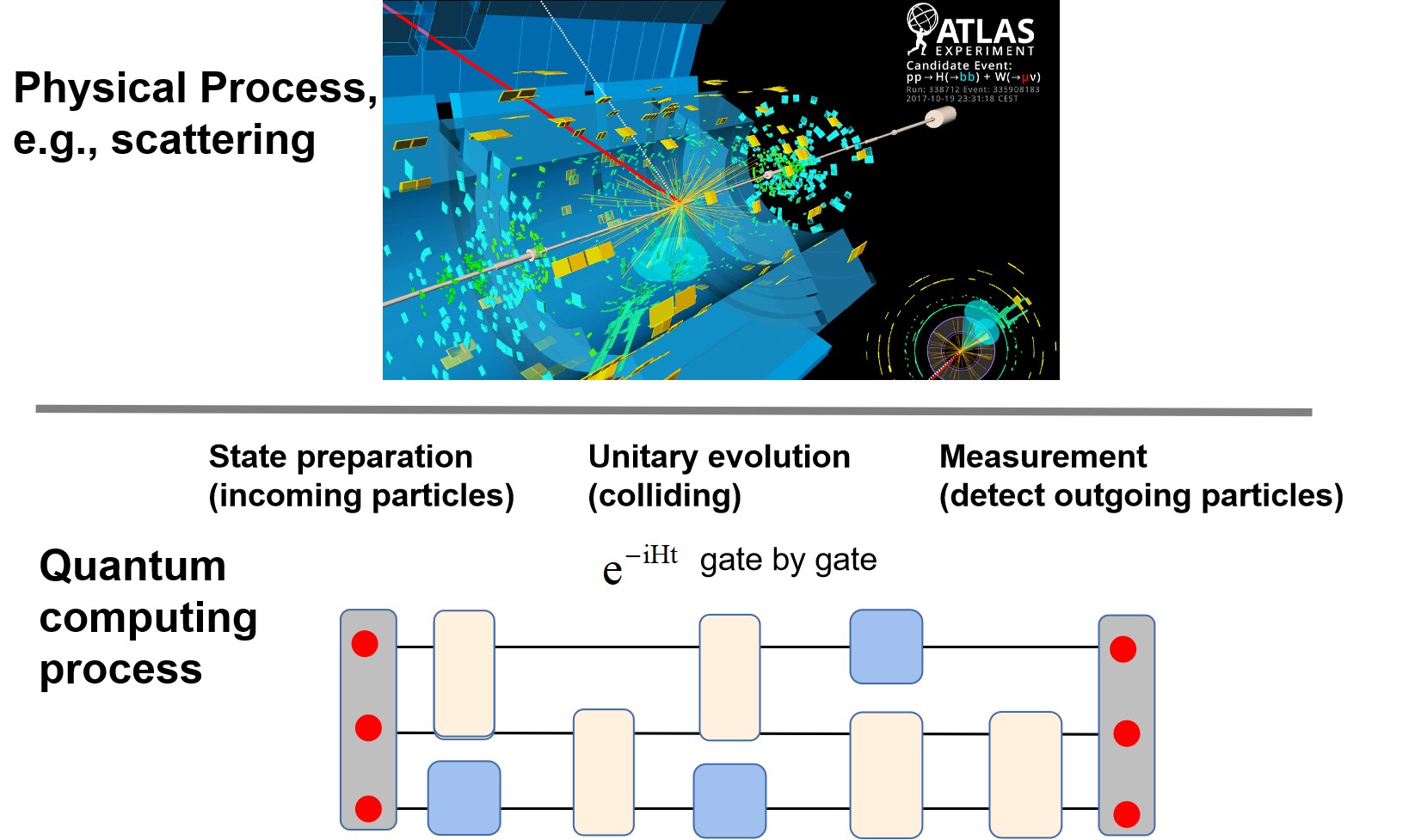
On a quantum computer, the basic unit to encode information is quantum bit, which can store a superposed state of and . In general, information is expressed as a quantum state of multiple qubtis. With several hundreds of qubits, a quantum computer can store a quantum state that is beyond the capacity of classical computers. The quantum state is manipulated on a quantum computer with unitary evolutions, which can be decoupled into a sequence of quantum gates from a universal set of basic quantum gates. Then, information or interested quantities can be extracted by repeatedly measuring the final quantum states. Further post-processing on a classical computer may be required. The physical process and its corresponding simulation on a quantum computer is illustrated in Fig. 1.
Nuclear physics includes problems related to steady states, such as structure of nucleons and phases of matter, and real-time evolution, such as scattering problem and evolution of nuclear matter. While preparation of steady states and simulating the real-time evolution have been standard techniques in quantum computing and variants of approaches have been developed, it is important to firstly convert nuclear physics into formulas that a quantum computer can handle with. Keep in mind that basic components of a quantum computer are qubits for encoding information, universal set of single and two-qubit quantum gates for manipulating information, and measurements for extracting information. To study nuclear physics on a quantum computer, those field operators should be converted into qubit operators, and the space-time should be discretized, and some symmetries should be considered, especially the local gauge invariance (general Gauss law). We discuss them separately.
Encode fields into qubits on lattice. Quantum fields usually are described on a continuous space-time and they can be bosonic (infinite dimension) or fermionic, while qubits on a quantum computer is defined on a lattice with each site resides one qubit. To encode quantum state of a quantum field on a quantum computer, we should discretize the space as a lattice, encode each local bosonic field into a finite number of qubits by a truncation, and encode a local fermionic field into a sequence of qubits by nonlocal transformations. Remarkably, to reduce the computational resource yet retain the essential physics, the discretization of space and the cut-off bosonic field should respect some physical arguments. In other words, the original nuclear physics problem may have an infinite degree of freedoms and it is important to map it into a task solvable on a quantum computer with a finite number of qubits under desired precision Jordan et al. (2012); Klco and Savage (2019). Another important ingredient in the encoding stage is how to express gauge field with qubits. It is important to enforce local gauge-invariance (general Gauss law) for simulating lattice gauge theory on a quantum computer Zohar et al. (2017a); Nu et al. (2019); Stryker (2019); Emonts and Zohar (2020) which corresponds to keep the simulation in the physical Hilbert space.
Unitary evolution. Physical processes in nuclear physics can be both unitary and nonunitary, while states on a quantum computer evolve in a unitary process. For an unitary evolution such as evolutions of the Hamiltonian, one can decompose the unitary operator into a sequence of basic single and two-qubit quantum gates with product-formula, by cutting the evolution time into short time periods. As an nonunitary process can be embedded in an unitary process of a larger system, one can introduce some auxiliary qubits to implement the nonunitary evolution. A common applied algorithmic design is by linear-combination-of-unitaries, using ancillary qubits Gui-Lu (2006); Childs et al. (2017); Van Apeldoorn et al. (2017); Chowdhury and Somma (2017); Gilyén et al. (2019); Arrazola et al. (2019) or continuous-variables Lau et al. (2017); Arrazola et al. (2019); Zhang et al. (2019, 2020a, 2020b).
Measurements. In nuclear physics, we often need to get distributions of particles, such as in the scattering problems. On a quantum computer, however, measurement often refer to computational basic ( measurements), which may not directly correspond to find particles in specified directions or momentums. One can synthesize such physical measurements by unitary evolutions followed by measurements on computational basis.
Digital vs analog quantum computer. It should be reminded of a difference between digital and analog quantum computers. Analog quantum computers are designed specifically for simulating quantum systems. Unlike a digital quantum computer that uses an universal set of quantum gates to construct all unitary process, an analog quantum computer can directly simulate a Hamiltonian and its real-time evolution, by engineering the desired interactions. This limits its capacity for simulating different systems, while on the other hand, it can be easier to implement. Representative physical systems for analog quantum computers include cold atoms Zhang et al. (2018b), trapped ions, and superconducting circuits. Nevertheless, analog quantum simulator can be programmable, enlarging its capacity of simulating a different target Hamiltonian with a controllable Hamiltonian on the physical platform using variational methods. For instance, ground state of the 1+1D Schwinger model has been simulated in the trapped-ion system with long-interaction between qubits Kokail et al. (2019).
II.2 Quantum algorithms for simulation
To exploit the power of quantum computers for simulating nuclear physics, quantum algorithms are indispensable. After having converting a nuclear physics problem on a quantum computer, the remaining task is to design a quantum algorithm to solve it efficiently. Although quantum algorithms can be counter-intuitive and requires special efforts to learn in general, it can be very natural for physicists when using quantum algorithms for solving quantum systems. Those quantum algorithms may be classified as two kinds: preparing steady states of a quantum system and simulating the real-time evolution. In the following, we give a brief introduction.
Simulating Hamiltonian evolutions is typically hard for classical computers, due to the growth of complexity of quantum states with increasing . However, it can be very directly implemented on a quantum computer, by decomposing into a set of quantum gates Lloyd (1996). For a Hamiltonian with local terms that for , the most basic technique is to use a product formula ( also named as Trotter formula), which is
| (1) |
For an desired precision , the time complexity is . It is interesting to note that while such a formula is simple, it is powerful even on the near-term quantum devices, and the performance can be comparable with more advanced quantum algorithms for Hamiltonian simulations Low and Chuang (2017); Campbell (2019); Childs et al. (2019). Remarkably, it is found that time-complexity can be reduced to using the product-formula when the Hamiltonian can be written as , where local terms in or commute to each other but . This is because there is a destructive error interference that errors will cancel in different short time periods Tran et al. (2020). This indicates product-formula may be more efficient than expected.
Solving steady states, including eigenstates and thermal states, is important for understanding static properties of quantum systems, but can be formidable challenge on a classical computer. Such a basic task is comparatively harder on a quantum computer than simulation of real-time evolution, and lots of efforts have been devoted into it. The first textbook algorithm is quantum phase estimation Nielsen and Chuang (2010), where eigenvalues of Hamiltonian are written onto ancillary qubits and then ancillary qubits are measured to read eigenvalue as well as associated eigenstates. Concretely, consider and the initial state is , then each eigenstate can be obtained with a probability . Thus it is important that the target eigenstate should have a large weighting in the initial state. Quantum phase estimation can be understood as signal processing from the time domain to the frequency domain. It involves Hamiltonian evolution at different time periods, and then uses quantum Fourier transformation to find eigenvalues at frequency domain. Both Hamiltonian evolution and quantum Fourier transformation are resource-costing, and consequently, quantum phase estimation is not suitable on the near-term quantum devices. Quantum adiabatic algorithm provides an approach to prepare ground state of a Hamiltonian Albash and Lidar (2018). It starts from a Hamiltonian whose ground state is easy to prepare, and by adiabatically tuning the Hamiltonian into the target Hamiltonian, the final state will be the ground state for the target Hamiltonian. The performance of the quantum adiabatic algorithm relies on a gap between the first excited state and the ground state along the adiabatic path. Thus it requires a good design for the adiabatic path which can be nontrivial. In practice, the adiabatic evolution should be very slow, and may be hard to finish within the coherent time. Thus, quantum adiabatic algorithm, although can be universal, may not be suitable in the era of NISQ.
Another important class of quantum algorithms is variational quantum eigensolver (VQE) Yung et al. (2014); McClean et al. (2016); Shen et al. (2017); Kandala et al. (2017); Hempel et al. (2018); Liu et al. (2019a); Kokail et al. (2019); Grimsley et al. (2019); Zhang and Yin (2020), which is considered promising for fully exploiting the power of NISQ quantum devices. It can rely on a shallow quantum circuit and a moderate number of qubits for solving classical intractable problems. The quantum circuit is parameterized and the parameters can be obtained by minimizing the energy. The optimization is a hybrid quantum-classical one. In this sense, variational quantum algorithms give a new paradigm for algorithmic design: rather than directly designing a quantum algorithm, it trains a quantum algorithm for a given task, by optimizing a cost function. The VQE is designed for solving the ground state by minimizing the energy, and variants of VQE have been developed for obtaining excited states McClean et al. (2017); Nakanishi et al. (2019); Higgott et al. (2019); Zhang et al. (2020c), thermal states at finite temperature Liu et al. (2019b); Wu and Hsieh (2019); Zhu et al. (2019); Chowdhury et al. (2020); Wang et al. (2020), quantum imaginary time evolution McArdle et al. (2019), and general quantum processes Endo et al. (2020).
III Applications for nuclear physics
Although at an early stage, quantum computing has had a broad applications for nuclear physics problems, and it is beyond the scope of this review for a throughout investigation. Rather, we attend to use some prototypical examples to illustrate how nuclear physics problems can be solved on a quantum computer. With concrete examples, the basic concepts and procedures may be revealed. We start with the 1+1D Schwinger model, which is a prototypical model for simulating gauge field with a state-of-art realistic quantum computer. Other examples include interesting problems ranging from scattering, evolution of non-equilibrium thermal states, nuclear structure at both high-energy and low-energy, and so on. In addition, we introduce a work that give the time complexity of solving scattering for a scalar quantum field, which shows quantum advantage.
III.1 Simulation of real-time evolution and ground state of lattice gauge theory: the Schwinger model
The capacity of quantum simulation of lattice gauge field implies that nuclear physics can be studied on a quantum computer. However, the required quantum resource is too demanding in the NISQ era, and it is more practical to start with some minimal models. The Schwinger model is such a prototypical model that has been demonstrated on current quantum devices, including both ground state Kokail et al. (2019) and real-time evolution Martinez et al. (2016). Moreover, the Schwinger model can reveal some important features shared with QCD. We thus use this model to illustrate a work flow for studying nuclear physics on a quantum computer: how the original formula of quantum field problem should be mapped into a lattice spin model, what quantum algorithm should be chosen to solve the lattice spin model, and how desired physical quantities can be accessed with measurements on a quantum computer, possible with post-processing.
We introduce the Hamiltonian for the Schwinger model with fixing gauge ,
| (2) |
where are fermionic field operators, the electric field and the vector potential satisfy and , and . In addition, the local conservation (Gauss law) should be respected, , which is a consequence of local gauge symmetry.
A recasting of Eq. (III.1) onto a lattice is the Kogut-Susskind formula Susskind (1977), which puts fermions on the sites and gauge field on bonds. Concretely, two-component fermions are defined on the even and odd sites respectively: and . Gauge fields on the bonds are and , which satisfy . By those representations, the lattice Hamiltonian under open boundary reads,
| (3) | |||||
The lattice Hamiltonian has already allowed for numeral simulation. Still, a challenge is to simulate the continuous variable gauge field with discrete-variable qubits. Approximations can be applied, either by reduction the to gauge field, or by a truncation into finite-dimension Hilbert space. Those can be standard schemes for all Abelian and non-Abelian gauge fields. Fortunately, the 1+1D Schwinger model is special as there is essentially no magnetic field. Moreover, the electric field and fermions are locally dependent into each other. This allows us to eliminate the gauge field totally by using the Gaussian law, , which determines , with as the value of at the left boundary. Now, the lattice model can be represented solely with fermionic operators, and by Jordan-Wigner transformation, , it can be written as a qubit Hamiltonian,
| (4) |
By eliminating the gauge field, the Hamiltonian is a bit more complicated as there are long-range interactions, but is still feasible on current quantum processors. Remarkably, trapped-ion quantum computers are renowned for its excellent connectivity, which is naturally suitable for simulating quantum systems with long-range interactions, while other platforms may suffer from limited connectivity. The following two experiments on trapped ions present the state-of-art simulations for the lattice gauge field on the real-time evolution and ground state properties, respectively.
Real-time evolution. Many nuclear physics phenomena involve time evolution and it is fundamentally important to simulate the real-time evolution of gauge theory. While existing classical methods often meet difficulties, simulation of real-time evolution can be implemented very naturally on a quantum computer, once an real-time evolution of a Hamiltonian is compiled into a sequence of quantum gates with Trotter decomposition. The Schwinger model was raised for explaining the mechanism of creating pairs of fermion-antifermion from the bare vacuum. Such a process can be simulated with a language of qubits. Firstly, occupation of a fermion (antifermion) is encoded as () on the even (odd) site. Then, the bare vacuum has no fermion at all, which can be represented as . With time evolution of the Hamiltonian, pairs of fermion-antifermion will appear due to hopping terms in the Hamiltonian. To implement on a quantum computer, a Trotter formula can decompose the time evolution into a product of short-time evolution of small Hamiltonian term, as in Eq. (1). Proliferation of fermion-antifermion pairs after a period of can be revealed by repeated measurements.
In trapped ions, a qubit is encoded as two internal energy levels in an ion. The experiment uses four ions to demonstrate the creation of fermion-antifermion pairs on realistic trapped-ion platforms, and the result fits good with theoretical results, with both idea evolution and the case of using the Trotter decomposition. Although with only a few qubits, this work has paved the way for simulating dynamical systems of large-scale systems that basically follows the same scheme.
Ground state. While real-time evolution for a system can be implemented directly on a quantum computer, solving its ground state or excited states requires more efforts on quantum algorithms. Variational quantum eigensolver provides a feasible scheme on the NISQ quantum processor. The key point is to train a quantum circuit to prepare a variational ground state for the target Hamiltonian , where parameters are optimized by minimizing the energy, . For the Schwinger model, one challenge is to adopt a wavefunction ansatz with enough expressive power under limited quantum resource, e.g., the parametrized quantum circuit should be shallow and yet can describe complicated quantum correlation of the ground state due to the long-range interactions. The current digital quantum computer is limited to small sizes as the required depths of quantum circuit can increase quickly with the system size. On the other hand, analog quantum simulator can realize an unitary operator by directly letting an engineered Hamiltonian evolves, which may be decomposed into a long sequence of quantum gates. Ref. Kokail et al. (2019) devises variational quantum simulator that can simulate the target Hamiltonian with engineered different Hamiltonian.
For simulating the Schwinger model with trapped-ions, an advantage is that engineered Hamiltonian of trapped-ions naturally have long-range interactions, which can be written as,
| (5) |
where , with that is tunable long-range interactions. Another engineered Hamiltonian required is that generates local rotation along axis. Those resource Hamiltonian can be applied to generate a trivial state via . An ansatz is to arrange odd layers as and even layers as performing independently on each qubit. The initial state is chosen as the bare vacuum state , corresponding to the ground state at . The ansatz always keep the state in the subspace of equal fermion and antifermion, which respects the symmetry of the ground state.
The parameter vector is trained by minimizing the variational energy . The optimization can be nontrivial for a noisy quantum processor, and it adopts a global optimizer called DIRECT Kokail et al. (2019), which divides the parameter space into cells for search. It is demonstrated that the trapped-ion simulator can variationally solving the ground state for up to 20 qubits for the Schwinger model, which is quite remarkable. Moreover, the experiment use zero energy variance to self-verifying that the obtained state is indeed the eigenstate, since an eigenstate can be characterized by zero energy variance. Although only shown with eight qubits, self-verifying can be vital for large-size quantum simulator that is beyond the computational capacity of classical computers: it requires the quantum computer itself to verify if it gives a result with enough accuracy. In addition, a quantum phase transition is revealed on the trapped-ion simulator by tuning the mass across (set and ). This indicates that the variational quantum simulator can efficiently solve ground states for the Schwinger model for a large range of parameters, especially around the quantum critical point where quantum correlations is strong. The work opens a new direction for simulating large-size quantum system exploiting analog quantum simulators with great flexibility by using the variational method.
We comment that elimination of the gauge field completely is only possible for 1+1D gauge theory. Nevertheless, the idea of reducing quantum resources for representing gauge field is important and possible, since gauge field has a redundancy in description. Many efforts have been denoted for this mapping stage, including non-Abelian gauge field in 1+1D Bañuls et al. (2017); Klco et al. (2020), 1+2D Abelian Zohar et al. (2017b) and non-Abelian gauge field, and so on .
III.2 Nuclear structure
One center motivation of nuclear physics is to explore the internal structure of nucleus, which relies on an increasing of energy scale of probes for resolving finer structures. Protons and neutrons are basic ingredients of a nucleus at low-energy scales, but a proton or a neutron itself is a collection of quarks and gluons at large energy scales. Colliders have been built for detecting those structures at different energy scales from scattering cross sections. Yet, numeral methods meet challenges that are common for quantum many-body systems, especially for solving the structure of hardrons, which in nature is non-perturbative. We review recent efforts for solving nuclear structure on a quantum computer Dumitrescu et al. (2018); Nu et al. (2020), for an atomic nucleus and an hadron respectively, which adopt quite different strategies.
III.2.1 Binding energy of atomic nucleus
From the aspect of low-energy nuclear physics, an atom consists of interacting protons and neutrons that are bounded together. Although lattice QCD can be applied, a better starting point is to use effective field theory (EFT) that protons and neutrons are relevant degree of freedoms. For light nucleus, pionless EFT provides systematically improvable approach for modeling nuclear interaction. For this bound-state problem, a second-quantization of the Hamiltonian can be obtained by using proper local basis, e.g., a common choice can be the harmonic oscillator basis. As a truncation of local basis can be applied, the problem can be solved in a finite-dimensional Hilbert space. Further, the second-quantization fermionic Hamiltonian can be mapped into a qubit Hamiltonian. Such a procedure is very familiar in quantum chemistry and quantum many-body problems in condensed matter. And one can immediately recognize that the problem is much like quantum chemistry, and it is expected that an exponential wall prevents classical methods when the system size is becoming large.
An interesting demonstration of quantum computing for atomic nucleus was reported in Ref. Dumitrescu et al. (2018), which adopts the VQE to solve the binding energy of the deuteron on a cloud quantum computer. With pionless EFT, the deuteron Hamiltonian with a truncation of basis reads,
| (6) |
where () create (annihilate) a deuteron in the harmonic-oscillator s-wave sate , and the hopping strength can be calculated under the harmonic oscillator basis. As the deuteron is described in EFT via a contact interaction, only nearest hopping exists (see Ref. Dumitrescu et al. (2018) for detailed values). By the Jordan-Wigner transformation, the Hamiltonian with increasing (up to ) can be written as,
With the harmonic oscillator basis, the deuteron ground state will be a superposition state at different basis, which is clear due to the hopping terms. The VQE approach uses an unitary-coupled-cluster (UCC) ansatz. Defining single excitation process, and , then we can employ ansatz for , for , both performing on the initial state . Parameters and are optimized by minimizing the energy of and with their corresponding variational wavefunciton, respectively. Further, the extrapolation to the infinite space should be employed with data obtained at finite size. The numeral results are shown to be very accurate with exact diagonalization.
We point out that solving the Hamiltonian in Eq. (6) is actually easy by exact diagonalization since it involves a tridiagonal matrix. Why bother to use a quantum computer? Moreover, a matrix is easy to diagonalize on a classical computer for , but can be challenge for the current quantum devices. It should be reminded that the VQE approach becomes valuable when solving nuclear structure becomes a many-body problem, and a simple exact diagonalization will face a matrix ( grows exponentially with ). It is expected that a road map for extending the scheme for quantum many-body nuclear physics is required.
III.2.2 Parton physics
Solving internal structure of a hadron is quite a different story. The partonic structure of a hadron depends on the energy scale to see it. For instance, a proton is a bounded state of three valence quarks at low energy scale, and no individual quark has been observed in experiments due to color confinement. On the other hand, at higher energy scale in deep inelastic scattering (DIS) with large momentum transfer, the hadron shall be modeled as a collection of charged point-like constituents, namely parton. The parton contributes to the cross section with momentum , where x is the momentum fraction of the proton carried by the parton, and is the momentum of the hadron. Understanding hadronic structure in terms of the parton distribution functions (PDFs) over and its generalization is a research frontier Ji (2013); Kang et al. (2014a, b); Lin et al. (2018).
The PDFs serve as an input for explaining scattering cross sections in DIS experiments. However, the parton distribution itself is hard to compute from ab initio methods due to its nonperturbative nature. There are different approaches from first principle, such as light-front Hamiltonian and lattice QCD, which still awaits for exascale supercomputer to verify. Here we introduce a recent work that points out an avenue on a near-term quantum computer.
Ref. Nu et al. (2020) presents two different schemes for calculating parton distribution on a quantum computer: direct calculation of PDFs using operator formula and by evaluation of the hadronic tensor. For illustration purpose two schemes are demonstrated with 1+1D Thirring model. The lattice Hamiltonian writes,
| (8) | |||||
where . This model is not gauge theory and thus is different from QCD. However, evaluating the hadronic tensor will not depend on the gauge field explicitly in lepton-hadron DIS at the leading order, and thus the second scheme is plausible and promising for studying PDF on NISQ quantum processors. The Hamiltonian shall be mapped into a spin model,
| (9) | |||||
Similar to the Schwinger model, the bare vacuum is set at limit, and () on the even (odd) site represents occupation of a fermion (antifermion), respectively.
The operator formula for a definition of PDF (without gauge link) is given by,
| (10) |
where and is the light-cone momentum for the incoming hadron. Noted that there is no Wilson line in the definition of Eq. (10) as gauge field is not involved in the Thirring model in Eq. (8). stands for the hadron state at momentum . In this sense, PDF is the Fourier transform of a time-separated correlator of the hadron. Two key procedures on a quantum computer are clear: firstly prepare which is a quantum many-body state for the Thirring model with quantum numbers for representing the hadron at momentum ; then calculate the correlator. Since there is only one flavor of fermion, we may express a hadron with a quantum number of three fermions, plus fluctuations of fermion-antifermion pairs. Such a scheme seems very straightforward, but some technical issues prevents it from being useful. Since light cone can not be defined on the lattice until the continuum limit, time-separated correlators should be evaluated with caution. The issue can be even more complicated for gauge theory where the Wilson line should be incorporated.
The second scheme exploits a connection between PDF and the hadronic tensor. The hadronic tensor for the -dimension theory is defined as correlations of currents ,
| (11) |
which can characterize the many-body wavefunction through correlations and consequently reveal the hadronic structure to some degree. The connection between PDF and is established as (via collinear factorization),
| (12) |
Here represents convolution, stands for parton species and is the partonic tensor. Thus, with , the parton distribution of species can be derived. The nontrivial relation between PDF and hadronic tensor is indicated in the convolution.
The remaining task is to evaluate on the state , which can refer to linear response method on a quantum computer. Still, the preparation of the state is quite involved, and Ref. Nu et al. (2020) points out that quantum adiabatic state preparation may be employed.
The above proposal suggests a way for studying parton physics on a quantum computer, but a demonstration is still awaited. This requires to efficiently prepare (possible with VQE), evaluating the hadronic tensor, and extracting PDF through global fitting to the results of hadronic tensor obtained from quantum computing. Another important question is which lattice Hamiltonian should be a good starting point. The light-front Hamiltonian of QCD looks promising as it already have provided a framework for ab initio calculation of proton structure. Remarkably, VQE based on the light-front Hamiltonian has just been demonstrated for calculating structure of pion Kreshchuk et al. (2020a).
III.3 Quantum advantage: scattering in scalar quantum field theory.
Scattering is central to nuclear physics as it is almost the only available experimental method. Consequently, calculating scattering amplitude is what in theory needed to do for a comparison with experiments. Different machinery of computational methods have been developed but there are some fundamental challenges. The difficulty can be revealed through a minimal model of quantum field theory, the theory, which is a scalar theory with quartic self-interactions. When the coupling approaches the phase transition point, the perturbative method becomes unreliable; and even in the weak-coupling regime, precision can be not controllable with the Feynman diagram calculation. Also, it is beyond the ability of lattice field theory which is good at calculating static properties, while scattering is a time-evolution problem. On the other hand, time-evolution can be implemented on a quantum computer and it is thus expected that scattering can be investigated efficiently.
A technical challenge is that the number of degree of freedom per unit volume is infinite, and it is necessary to give a mapping that can assign qubits to physical degree of freedom, in a controllable way under desired accuracy. For instance, truncation of Fock space can be applied, since the number of particles is constrained by the energy of incoming particles. Then, given the number of qubits, preparation of incoming two particles as two wave packets, and their scattering, should be formulated in the language of quantum circuit. The quantum advantage is that the depth of the quantum circuit scales only polynomial with the number of particles, energy and the desired precision, for both weak and strong couplings Jordan et al. (2012).
The space is discretized as a d-dimensional lattice with lattice spacing . Let us start with the lattice Hamiltonian,
| (13) | |||||
Here is field operator on the site , is the conjugate field satisfying , is a finite-difference operator, is the particle mass for the non-interacting theory corresponding to .
The first issue is to represent the infinite dimensional field in terms of qubits. Setting as a cutoff and as increments, qubits are required per site. With a constraint of energy , the cutoff is for desired fidelity to the original state. The energy constraint also introduce a cutoff to . Note that as and are conjugate. Then, it follows that .
Two incoming particles should be expressed as a many-body initial state with two separated wave packets on the lattice. The initial state can be prepared in an adiabatic way, which involves two steps: firstly, two separated wave packets are produced on the vacuum of the non-interacting Hamiltonian , where the vacuum is a Gaussian state and can be constructed exactly; Secondly, interaction is turned on and the system evolves adiabatically with Hamiltonian parameterized by , where , and is the adiabatic path. Note that the wave packets will propagate and broaden since it is not an eigenstate of , additional backward evolution is required to undo unnecessary dynamical phases. The time complexity for the initial state procedure scales as . The system of two incoming particles then evolves for a period that scattering occurs. Then, the interaction is adiabatic turn-off and the scattering result is sampled by measuring the number operator of momentum modes defined in the free theory. With scaling analysis via effective field theory, the algorithm shows a complexity polynomial with the , e.g., in 1D its . Remarkably, at strong coupling, the time complexity still scales polynomial with ( is the quantum phase transition point), the momentum of incoming particles , the maximum kinematically allowed number of outgoing particles and the precision . This is in contrast to the known classical algorithm scaling exponentially with and , thus showing an exponentially quantum speed-up.
The merit of this work is to make clear the point of solving quantum field theory on a quantum computer with quantum advantage. A scheme to reach this goal has also been pointed out. Still, some subroutines may be improved to make the algorithm more implementable in the NISQ era, and there indeed are some following jobs with more detailed algorithms Klco and Savage (2019).
III.4 Non-equilibrium dynamics
In physics we often need to study non-equilibrium quantum systems at finite temperature. For nuclear physics, quark-gluon plasma, which is produced in heavy-ion collision or in the expansion of the early Universe, is an outstanding example but still limited knowledge is known, as simulation with classical methods are very hard. Basically, studies of such quantum systems involves time evolution of density matrix. As a quantum computer essentially manipulate pure quantum states with unitary operation, an extension to density matrix needs additional treatment. One can either refer to a subsystem by tracing out the ancillary, or view the density matrix as an ensemble of pure quantum states with a classical distribution.
Consider a density matrix as the initial state for a quantum system, then its real-time evolution under is given by . The initial state can be set as equilibrium state for the system under at inverse temperature , namely quantum Gibbs state, , which satisfying the symmetric Bloch equation,
| (14) |
with initial condition . In Ref. Lamm and Lawrence (2018), a hybrid quantum-classical scheme has been developed for the real-time evolution of density matrix in the context of nuclear physics. The initial state is obtained by solving Eq. (14) with density matrix quantum Monte Carlo algorithm (DMQMC), leading to an approximation of , with . Such an approximation is completed on a classical computer with enough samples of . With the approximated initial state, time-dependent observable is evaluated as (with a substitution ),
The task thus can be decomposed to evaluate observable for each component, including the diagonal term, e.g., , and the off-diagonal term, such as . The former corresponds to perform measurement on a state evolved with from initial state or . And for the later, one can replace initial state with .
In total, the hybrid quantum-classical approach adopts a strategy that assign quantum resource for the real-time evolution part which is hard for the classical computer, while the classical part can utilize the state-of-art classical algorithm since it is good at solving steady states. A combination of both makes this approach promising on NISQ quantum processors for studying non-equilibrium dynamics.
IV Outlook and summary
At this stage, we have given an introductory review of quantum computing for nuclear physics, but a throughout investigation is still beyond the scope of this review, given recent rapid expanding of this field. We further briefly give an outlook that focuses on this field within the NISQ era. Although formulations of lattice gauge theory for quantum computing have been developed in a few different approaches, it is clear that there still is a considerable gap for simulating QCD on NISQ quantum processors with limited quantum resources, and it is anticipated that more efficient schemes of expressing degree of freedom of gauge field and its coupling to matter field would be developed. On the other hand, incorporating quantum algorithms as subroutines into a hybrid quantum-classical algorithm can be a very promising approach for solving nuclear physics with practical results.
Another observation is that there is still a lack of consensus on the goal; perhaps it is inspiring that a road-map can be proposed for demonstrating quantum advantages for nuclear physics on a quantum computer, in accordance with the scaling-up of near-term quantum processors and error mitigation techniques . Moreover, software methodology is important, as it enables systematic developments and rapid innovations on both quantum algorithms and applications to nuclear physics. Compared with quantum computing for chemistry McClean et al. (2020) and quantum machine learning Bergholm et al. (2020), open-source packages are still lacked for nuclear physics, and it awaits for such packages for making an attempt to study nuclear physics on a quantum computer more friendly.
In summary, we have given an brief review on recent advances on quantum computing for nuclear physics. We have clarified two different approaches from analog and digital quantum simulator, and the review has focused on the latter. We have outlined how degrees of freedom of nuclear physics problems can be mapped into a formula of qubits that is solvable on a quantum computer, and the corresponding quantum algorithms for both static properties and real-time evolution have been shortly discussed. Concretely, we have given some examples from recent outstanding works, ranging from simulation of lattice gauge theory, nuclear structure as well as quantum advantage in terms of time complexity for scattering problem. Lastly, we have pointed out that lots of efforts are still required to make quantum computing a playground for investigating nuclear physics on near-term quantum devices.
Acknowledgements.
This work was supported by the Key-Area Research and Development Program of GuangDong Province (Grant No. 2019B030330001), the National Key Research and Development Program of China (Grant No. 2016YFA0301800), the National Natural Science Foundation of China (Grants No. 12005065, No.12022512, No.12035007, and No. 12074180), and the Key Project of Science and Technology of Guangzhou (Grants No. 201804020055 and No. 2019050001).References
- Peskin and Schroeder (1995) M. Peskin and D. Schroeder, “An introduction to quantum field theory,” (1995).
- Wilson (1974) Kenneth G. Wilson, “Confinement of quarks,” Phys. Rev. D 10, 2445–2459 (1974).
- Kogut and Susskind (1975) J. Kogut and L. Susskind, “Hamiltonian formulation of wilson’s lattice gauge theories,” Phys. Rev. 11, 395 (1975).
- Kogut (1983) John B. Kogut, “The lattice gauge theory approach to quantum chromodynamics,” Rev. Mod. Phys. 55, 775–836 (1983).
- McLerran and Svetitsky (1981) L. D. McLerran and B. Svetitsky, “A monte carlo study of su(2) yang-mills theory at finite temperature,” Phys. Lett. 98, 195 (1981).
- Troyer and Wiese (2005) M. Troyer and U. J. Wiese, “Computational complexity and fundamental limitations to fermionic quantum monte carlo simulations,” Phys. Rev. Lett. 94 (2005).
- Silvi et al. (2014) Pietro Silvi, Enrique Rico, Tommaso Calarco, and Simone Montangero, “Lattice gauge tensor networks,” New Journal of Physics 16, 103015 (2014).
- Tagliacozzo et al. (2014) L. Tagliacozzo, A. Celi, and M. Lewenstein, “Tensor networks for lattice gauge theories with continuous groups,” Physical Review X 4, 041024 (2014).
- Rico et al. (2014) E. Rico, T. Pichler, M. Dalmonte, P. Zoller, and S. Montangero, “Tensor networks for lattice gauge theories and atomic quantum simulation,” Phys. Rev. Lett. 112, 201601 (2014).
- Kühn et al. (2015) Stefan Kühn, Erez Zohar, J. Ignacio Cirac, and Mari Carmen Bañuls, “Non-abelian string breaking phenomena with matrix product states,” J. High Energy Phys. 2015, 130 (2015).
- Buyens et al. (2016) Boye Buyens, Frank Verstraete, and Karel Van Acoleyen, “Hamiltonian simulation of the schwinger model at finite temperature,” Phys. Rev. D 94, 085018 (2016).
- Bañuls et al. (2017) Mari Carmen Bañuls, Krzysztof Cichy, J. Ignacio Cirac, Karl Jansen, and Stefan Kühn, “Efficient basis formulation for ()-dimensional su(2) lattice gauge theory: Spectral calculations with matrix product states,” Physical Review X 7, 041046 (2017).
- Silvi et al. (2019) Pietro Silvi, Yannick Sauer, Ferdinand Tschirsich, and Simone Montangero, “Tensor network simulation of an su(3) lattice gauge theory in 1d,” Phys. Rev. D 100, 074512 (2019).
- Emonts and Zohar (2020) Patrick Emonts and Erez Zohar, “Gauss Law, Minimal Coupling and Fermionic PEPS for Lattice Gauge Theories,” SciPost Phys. Lect. Notes , 12 (2020).
- Feynman (1982) R. Feynman, “Simulating physics with computers,” Int. J. Theor. Phys. 21, 467 (1982).
- Lloyd (1996) S. Lloyd, “Universal quantum simulators,” Science 273, 1073 (1996).
- Preskill (2018) John Preskill, “Quantum Computing in the NISQ era and beyond,” Quantum 2, 79 (2018), arXiv: 1801.00862.
- Yung et al. (2014) M. H. Yung, J. Casanova, A. Mezzacapo, J. McClean, L. Lamata, A. Aspuru-Guzik, and E. Solano, “From transistor to trapped-ion computers for quantum chemistry,” Scientific Reports 4, 3589 (2014).
- McClean et al. (2016) Jarrod R. McClean, Jonathan Romero, Ryan Babbush, and Alán Aspuru-Guzik, “The theory of variational hybrid quantum-classical algorithms,” New Journal of Physics 18, 023023 (2016).
- O’Malley et al. (2016) P. J J O’Malley, R. Babbush, I. D Kivlichan, J. Romero, J. R McClean, R. Barends, J. Kelly, P. Roushan, A. Tranter, N. Ding, B. Campbell, Y. Chen, Z. Chen, B. Chiaro, A. Dunsworth, A. G Fowler, E. Jeffrey, E. Lucero, A. Megrant, J. Y Mutus, M. Neeley, C. Neill, C. Quintana, D. Sank, A. Vainsencher, J. Wenner, T. C White, P. V Coveney, P. J Love, H. Neven, A. Aspuru-Guzik, and J. M Martinis, “Scalable quantum simulation of molecular energies,” Physical Review X 6, 031007 (2016).
- Kandala et al. (2017) Abhinav Kandala, Antonio Mezzacapo, Kristan Temme, Maika Takita, Markus Brink, Jerry M. Chow, and Jay M. Gambetta, “Hardware-efficient variational quantum eigensolver for small molecules and quantum magnets,” Nature 549, 242–246 (2017).
- Grimsley et al. (2019) Harper R. Grimsley, Sophia E. Economou, Edwin Barnes, and Nicholas J. Mayhall, “An adaptive variational algorithm for exact molecular simulations on a quantum computer,” Nature Communications 10, 3007 (2019).
- Arute et al. (2020) Frank Arute et al., “Hartree-fock on a superconducting qubit quantum computer,” (2020), arXiv:2004.04174 [quant-ph] .
- Liu et al. (2019a) Jin-Guo Liu, Yi-Hong Zhang, Yuan Wan, and Lei Wang, “Variational quantum eigensolver with fewer qubits,” Phys. Rev. Research 1, 023025 (2019a).
- Kokail et al. (2019) C. Kokail, C. Maier, R. van Bijnen, T. Brydges, M. K. Joshi, P. Jurcevic, C. A. Muschik, P. Silvi, R. Blatt, C. F. Roos, and P. Zoller, “Self-verifying variational quantum simulation of lattice models,” Nature 569, 355–360 (2019).
- Dallaire-Demers et al. (2020) Pierre-Luc Dallaire-Demers, Michał Stęchły, Jerome F. Gonthier, Ntwali Toussaint Bashige, Jonathan Romero, and Yudong Cao, “An application benchmark for fermionic quantum simulations,” (2020), arXiv:2003.01862 [quant-ph] .
- Anschuetz et al. (2018) Eric R. Anschuetz, Jonathan P. Olson, Alán Aspuru-Guzik, and Yudong Cao, “Variational quantum factoring,” arXiv:1808.08927 (2018).
- Xu et al. (2019) Xiaosi Xu, Jinzhao Sun, Suguru Endo, Ying Li, Simon C. Benjamin, and Xiao Yuan, “Variational algorithms for linear algebra,” (2019), arXiv:1909.03898 [quant-ph] .
- Lubasch et al. (2020) Michael Lubasch, Jaewoo Joo, Pierre Moinier, Martin Kiffner, and Dieter Jaksch, “Variational quantum algorithms for nonlinear problems,” Phys. Rev. A 101, 010301 (2020).
- Nu et al. (2019) Q. S. Collaboration Nu, Henry Lamm, Scott Lawrence, and Yukari Yamauchi, “General methods for digital quantum simulation of gauge theories,” Phys. Rev. D 100, 034518 (2019).
- Zohar et al. (2017a) Erez Zohar, Alessandro Farace, Benni Reznik, and J. Ignacio Cirac, “Digital lattice gauge theories,” Phys. Rev. A 95, 023604 (2017a).
- Stryker (2019) Jesse R. Stryker, “Oracles for gauss’s law on digital quantum computers,” Phys. Rev. A 99, 042301 (2019).
- Halimeh and Hauke (2020) Jad C. Halimeh and Philipp Hauke, “Reliability of Lattice Gauge Theories,” Phys. Rev. Lett. 125, 030503 (2020).
- Büchler et al. (2005) H. P. Büchler, M. Hermele, S. D. Huber, Matthew P. A. Fisher, and P. Zoller, “Atomic quantum simulator for lattice gauge theories and ring exchange models,” Phys. Rev. Lett. 95, 040402 (2005).
- Lewenstein M and Sen (2007) Sanpera A. Ahufinger V. Damski B. Sen A. Lewenstein M and U. Sen, “Ultracold atomic gases in optical lattices: mimicking condensed matter physics and beyond,” Adv. Phys. 56, 243 (2007).
- Boada O and Pico (2010) Celi A. Latorre J. I. Boada O and V. Pico, “Simulation of gauge transformations on systems of ultracold atoms,” New J. Phys. 12 (2010).
- Bermudez et al. (2010) A. Bermudez, L. Mazza, M. Rizzi, N. Goldman, M. Lewenstein, and M. A. Martin-Delgado, “Wilson fermions and axion electrodynamics in optical lattices,” Phys. Rev. Lett. 105, 190404 (2010).
- Banerjee D and Zoller (2012) Dalmonte M. Müller M. Rico E. Stebler P. Wiese U. J. Banerjee D and P. Zoller, “Atomic quantum simulation of dynamical gauge fields coupled to fermionic matter: from string breaking to evolution after a quench,” Phys. Rev. Lett. 109 (2012).
- Zohar E and Reznik (2012) Cirac J. I. Zohar E and B. Reznik, “Simulating compact quantum electrodynamics with ultracold atoms: Probing confinement and nonperturbative effects,” Phys. Rev. Lett. 109 (2012).
- Zohar E and Reznik (2013) Cirac J. I. Zohar E and B. Reznik, “Simulating (2+1)-dimensional lattice qed with dynamical matter using ultracold atoms,” Phys. Rev. Lett. 110 (2013).
- Zohar et al. (2013) Erez Zohar, J. Ignacio Cirac, and Benni Reznik, “Cold-atom quantum simulator for su(2) yang-mills lattice gauge theory,” Phys. Rev. Lett. 110, 125304 (2013).
- Zohar et al. (2015) Erez Zohar, J. Ignacio Cirac, and Benni Reznik, “Quantum simulations of lattice gauge theories using ultracold atoms in optical lattices,” Rep. Prog. Phys. 79, 014401 (2015).
- Stannigel et al. (2014) K. Stannigel, P. Hauke, D. Marcos, M. Hafezi, S. Diehl, M. Dalmonte, and P. Zoller, “Constrained dynamics via the zeno effect in quantum simulation: Implementing non-abelian lattice gauge theories with cold atoms,” Phys. Rev. Lett. 112, 120406 (2014).
- Görg et al. (2019) Frederik Görg, Kilian Sandholzer, Joaquín Minguzzi, Rémi Desbuquois, Michael Messer, and Tilman Esslinger, “Realization of density-dependent peierls phases to engineer quantized gauge fields coupled to ultracold matter,” Nat. Phys. 15, 1161–1167 (2019).
- Mil et al. (2020) Alexander Mil, Torsten V. Zache, Apoorva Hegde, Andy Xia, Rohit P. Bhatt, Markus K. Oberthaler, Philipp Hauke, Jürgen Berges, and Fred Jendrzejewski, “A scalable realization of local u(1) gauge invariance in cold atomic mixtures,” Science 367, 1128 (2020).
- Blatt and Roos (2012) R. Blatt and C. F. Roos, “Quantum simulations with trapped ions,” Nat. Phys. 8, 277 (2012).
- Hauke P and Zoller (2013) Marcos D. Dalmonte M. Hauke P and P. Zoller, “Quantum simulation of a lattice schwinger model in a chain of trapped ions,” Phys. Rev. 3 (2013).
- Martinez et al. (2016) Esteban A. Martinez, Christine A. Muschik, Philipp Schindler, Daniel Nigg, Alexander Erhard, Markus Heyl, Philipp Hauke, Marcello Dalmonte, Thomas Monz, Peter Zoller, and Rainer Blatt, “Real-time dynamics of lattice gauge theories with a few-qubit quantum computer,” Nature 534, 516–519 (2016).
- Clark et al. (2018) Logan W. Clark, Brandon M. Anderson, Lei Feng, Anita Gaj, K. Levin, and Cheng Chin, “Observation of density-dependent gauge fields in a bose-einstein condensate based on micromotion control in a shaken two-dimensional lattice,” Phys. Rev. Lett. 121, 030402 (2018).
- Davoudi et al. (2020a) Zohreh Davoudi, Mohammad Hafezi, Christopher Monroe, Guido Pagano, Alireza Seif, and Andrew Shaw, “Towards analog quantum simulations of lattice gauge theories with trapped ions,” Physical Review Research 2, 023015 (2020a).
- Marcos D and Zoller (2013) Rabl P. Rico E. Marcos D and P. Zoller, “Superconducting circuits for quantum simulation of dynamical gauge fields,” Phys. Rev. Lett. 111 (2013).
- Marcos et al. (2014) D. Marcos, P. Widmer, E. Rico, M. Hafezi, P. Rabl, U. J. Wiese, and P. Zoller, “Two-dimensional lattice gauge theories with superconducting quantum circuits,” Ann. Phys-new. York. 351, 634–654 (2014).
- Tagliacozzo L and Lewenstein (2013) Celi A. Zamora A. Tagliacozzo L and M. Lewenstein, “Optical abelian lattice gauge theories,” Ann. Phys. 330, 160 (2013).
- Tagliacozzo et al. (2013) L. Tagliacozzo, A. Celi, P. Orland, M. W. Mitchell, and M. Lewenstein, “Simulation of non-abelian gauge theories with optical lattices,” Nature Communications 4, 2615 (2013).
- Zhang et al. (2018a) Jin Zhang, J. Unmuth-Yockey, J. Zeiher, A. Bazavov, S. W. Tsai, and Y. Meurice, “Quantum simulation of the universal features of the polyakov loop,” Phys. Rev. Lett. 121, 223201 (2018a).
- Bernien et al. (2017) Hannes Bernien, Sylvain Schwartz, Alexander Keesling, Harry Levine, Ahmed Omran, Hannes Pichler, Soonwon Choi, Alexander S. Zibrov, Manuel Endres, Markus Greiner, Vladan Vuletić, and Mikhail D. Lukin, “Probing many-body dynamics on a 51-atom quantum simulator,” Nature 551, 579–584 (2017).
- Surace et al. (2020) Federica M. Surace, Paolo P. Mazza, Giuliano Giudici, Alessio Lerose, Andrea Gambassi, and Marcello Dalmonte, “Lattice gauge theories and string dynamics in rydberg atom quantum simulators,” Physical Review X 10, 021041 (2020).
- Wiese (2013) U. J. Wiese, “Ultracold quantum gases and lattice systems: quantum simulation of lattice gauge theories,” Ann. Phys. 525, 777 (2013).
- Zhang et al. (2018b) Dan-Wei Zhang, Yan-Qing Zhu, Y. X. Zhao, Hui Yan, and Shi-Liang Zhu, “Topological quantum matter with cold atoms,” Advances in Physics 67, 253–402 (2018b).
- Zhang et al. (2011) D. W. Zhang, Z. D. Wang, and S.-L. Zhu, “Relativistic quantum effects of dirac particles simulated by ultracold atoms,” Frontiers of Physics 7, 31–53 (2011).
- Jordan et al. (2012) Stephen P. Jordan, Keith S. M. Lee, and John Preskill, “Quantum algorithms for quantum field theories,” Science 336, 1130–1133 (2012).
- Notarnicola S and Pepe (2015) Ercolessi E. Facchi P. Marmo G. Pascazio S. Notarnicola S and F. V. Pepe, “Discrete abelian gauge theories for quantum simulations of qed,” J. Phys. A: Math. Theor. 48 (2015).
- Lamm and Lawrence (2018) Henry Lamm and Scott Lawrence, “Simulation of nonequilibrium dynamics on a quantum computer,” Phys. Rev. Lett. 121, 170501 (2018).
- Klco et al. (2018) N. Klco, E. F. Dumitrescu, A. J. McCaskey, T. D. Morris, R. C. Pooser, M. Sanz, E. Solano, P. Lougovski, and M. J. Savage, “Quantum-classical computation of schwinger model dynamics using quantum computers,” Phys. Rev. A 98, 032331 (2018).
- Nu et al. (2020) Q. S. Collaboration Nu, Henry Lamm, Scott Lawrence, and Yukari Yamauchi, “Parton physics on a quantum computer,” Physical Review Research 2, 013272 (2020).
- Klco and Savage (2019) Natalie Klco and Martin J. Savage, “Digitization of scalar fields for quantum computing,” Phys. Rev. A 99, 052335 (2019).
- Klco et al. (2020) Natalie Klco, Martin J. Savage, and Jesse R. Stryker, “Su(2) non-abelian gauge field theory in one dimension on digital quantum computers,” Phys. Rev. D 101, 074512 (2020).
- Yeter-Aydeniz et al. (2019) Kübra Yeter-Aydeniz, Eugene F. Dumitrescu, Alex J. McCaskey, Ryan S. Bennink, Raphael C. Pooser, and George Siopsis, “Scalar quantum field theories as a benchmark for near-term quantum computers,” Phys. Rev. A 99, 032306 (2019).
- Zohar et al. (2017b) Erez Zohar, Alessandro Farace, Benni Reznik, and J. Ignacio Cirac, “Digital quantum simulation of lattice gauge theories with dynamical fermionic matter,” Phys. Rev. Lett. 118, 070501 (2017b).
- Zohar and Cirac (2018) Erez Zohar and J. Ignacio Cirac, “Eliminating fermionic matter fields in lattice gauge theories,” Phys. Rev. B 98, 075119 (2018).
- Bauer et al. (2019) Christian W. Bauer, Wibe A. de Jong, Benjamin Nachman, and Davide Provasoli, “A quantum algorithm for high energy physics simulations,” arXiv:1904.03196 [hep-ph, physics:quant-ph] (2019), arXiv: 1904.03196.
- Raychowdhury and Stryker (2020) Indrakshi Raychowdhury and Jesse R. Stryker, “Loop, string, and hadron dynamics in su(2) hamiltonian lattice gauge theories,” Phys. Rev. D 101, 114502 (2020).
- Du et al. (2020) Weijie Du, James P. Vary, Xingbo Zhao, and Wei Zuo, “Quantum Simulation of Nuclear Inelastic Scattering,” arXiv:2006.01369 [nucl-th, physics:quant-ph] (2020), arXiv: 2006.01369.
- Roggero et al. (2020) Alessandro Roggero, Andy C.Y. Li, Joseph Carlson, Rajan Gupta, and Gabriel N. Perdue, “Quantum computing for neutrino-nucleus scattering,” Phys. Rev. D 101, 074038 (2020).
- Kreshchuk et al. (2020a) Michael Kreshchuk, Shaoyang Jia, William M. Kirby, Gary Goldstein, James P. Vary, and Peter J. Love, “Light-Front Field Theory on Current Quantum Computers,” arXiv:2009.07885 [hep-lat, physics:hep-th, physics:quant-ph] (2020a), arXiv: 2009.07885.
- de Jong et al. (2020) Wibe A. de Jong, Mekena Metcalf, James Mulligan, Mateusz Płoskoń, Felix Ringer, and Xiaojun Yao, “Quantum simulation of open quantum systems in heavy-ion collisions,” arXiv:2010.03571 [hep-ex, physics:hep-ph, physics:nucl-ex, physics:nucl-th, physics:quant-ph] (2020), arXiv: 2010.03571.
- Davoudi et al. (2020b) Zohreh Davoudi, Indrakshi Raychowdhury, and Andrew Shaw, “Search for Efficient Formulations for Hamiltonian Simulation of non-Abelian Lattice Gauge Theories,” (2020b), arXiv:2009.11802 [hep-lat] .
- Wei et al. (2020) Annie Y. Wei, Preksha Naik, Aram W. Harrow, and Jesse Thaler, “Quantum algorithms for jet clustering,” Phys. Rev. D 101, 094015 (2020).
- Klco and Savage (2020) Natalie Klco and Martin J. Savage, “Fixed-Point Quantum Circuits for Quantum Field Theories,” arXiv:2002.02018 [hep-th, physics:nucl-th, physics:quant-ph] (2020), arXiv: 2002.02018.
- Holland et al. (2020) Eric T. Holland, Kyle A. Wendt, Konstantinos Kravvaris, Xian Wu, W. Erich Ormand, Jonathan L DuBois, Sofia Quaglioni, and Francesco Pederiva, “Optimal control for the quantum simulation of nuclear dynamics,” Phys. Rev. A 101, 062307 (2020).
- Avkhadiev et al. (2020) A. Avkhadiev, P.E. Shanahan, and R.D. Young, “Accelerating Lattice Quantum Field Theory Calculations via Interpolator Optimization Using Noisy Intermediate-Scale Quantum Computing,” Phys. Rev. Lett. 124, 080501 (2020).
- Kharzeev and Kikuchi (2020) Dmitri E. Kharzeev and Yuta Kikuchi, “Real-time chiral dynamics from a digital quantum simulation,” Phys. Rev. Research 2, 023342 (2020).
- Shaw et al. (2020) Alexander F. Shaw, Pavel Lougovski, Jesse R. Stryker, and Nathan Wiebe, “Quantum Algorithms for Simulating the Lattice Schwinger Model,” Quantum 4, 306 (2020), arXiv: 2002.11146.
- Liu and Xin (2020) Junyu Liu and Yuan Xin, “Quantum simulation of quantum field theories as quantum chemistry,” arXiv:2004.13234 [hep-th, physics:quant-ph] (2020), arXiv: 2004.13234.
- Mueller et al. (2020) Niklas Mueller, Andrey Tarasov, and Raju Venugopalan, “Deeply inelastic scattering structure functions on a hybrid quantum computer,” Phys. Rev. D 102, 016007 (2020).
- Bepari et al. (2020) Khadeejah Bepari, Sarah Malik, Michael Spannowsky, and Simon Williams, “Towards a Quantum Computing Algorithm for Helicity Amplitudes and Parton Showers,” arXiv:2010.00046 [hep-ex, physics:hep-ph, physics:quant-ph] (2020), arXiv: 2010.00046.
- Kreshchuk et al. (2020b) Michael Kreshchuk, William M. Kirby, Gary Goldstein, Hugo Beauchemin, and Peter J. Love, “Quantum Simulation of Quantum Field Theory in the Light-Front Formulation,” arXiv:2002.04016 [hep-th, physics:quant-ph] (2020b), arXiv: 2002.04016.
- Nielsen and Chuang (2010) Michael A. Nielsen and Isaac L. Chuang, Quantum Computation and Quantum Information: 10th Anniversary Edition (Cambridge University Press, 2010).
- Muschik et al. (2017) Christine Muschik, Markus Heyl, Esteban Martinez, Thomas Monz, Philipp Schindler, Berit Vogell, Marcello Dalmonte, Philipp Hauke, Rainer Blatt, and Peter Zoller, “U(1) wilson lattice gauge theories in digital quantum simulators,” New Journal of Physics 19, 103020 (2017).
- Gui-Lu (2006) Long Gui-Lu, “General quantum interference principle and duality computer,” Commun. Theor. Phys. 45, 825–844 (2006).
- Childs et al. (2017) Andrew M. Childs, Robin Kothari, and Rolando D. Somma, “Quantum algorithm for systems of linear equations with exponentially improved dependence on precision,” Siam. J. Comput. 46, 1920–1950 (2017).
- Van Apeldoorn et al. (2017) J. Van Apeldoorn, A. Gilyen, S. Gribling, and R. de Wolf, “Quantum sdp-solvers: better upper and lower bounds,” 2017 IEEE 58th Annual Symposium on Foundations of Computer Science (FOCS). Proceedings , 403–414 (2017).
- Chowdhury and Somma (2017) Anirban Narayan Chowdhury and Rolando D. Somma, “Quantum algorithms for gibbs sampling and hitting-time estimation,” Quantum Information & Computation 17, 41–64 (2017).
- Gilyén et al. (2019) András Gilyén, Yuan Su, Guang Hao Low, and Nathan Wiebe, “Quantum singular value transformation and beyond: Exponential improvements for quantum matrix arithmetics,” in Proceedings of the 51st Annual ACM SIGACT Symposium on Theory of Computing, STOC 2019 (Association for Computing Machinery, New York, NY, USA, 2019) p. 193–204.
- Arrazola et al. (2019) Juan Miguel Arrazola, Timjan Kalajdzievski, Christian Weedbrook, and Seth Lloyd, “Quantum algorithm for nonhomogeneous linear partial differential equations,” Phys. Rev. A 100, 032306 (2019).
- Lau et al. (2017) H. K. Lau, R. Pooser, G. Siopsis, and C. Weedbrook, “Quantum machine learning over infinite dimensions,” Phys. Rev. Lett. 118, 080501 (2017).
- Zhang et al. (2019) Dan-Bo Zhang, Zheng-Yuan Xue, Shi-Liang Zhu, and Z. D. Wang, “Realizing quantum linear regression with auxiliary qumodes,” Phys. Rev. A 99, 012331 (2019).
- Zhang et al. (2020a) Dan-Bo Zhang, Shi-Liang Zhu, and Z. D. Wang, “Protocol for implementing quantum nonparametric learning with trapped ions,” Phys. Rev. Lett. 124, 010506 (2020a).
- Zhang et al. (2020b) Dan-Bo Zhang, Guo-Qing Zhang, Zheng-Yuan Xue, Shi-Liang Zhu, and Z. D. Wang, “Continuous-variable assisted thermal quantum simulation,” (2020b), arXiv:2006.00471 [quant-ph] .
- Low and Chuang (2017) Guang Hao Low and Isaac L. Chuang, “Optimal hamiltonian simulation by quantum signal processing,” Phys. Rev. Lett. 118, 010501 (2017).
- Campbell (2019) Earl Campbell, “Random compiler for fast hamiltonian simulation,” Phys. Rev. Lett. 123, 070503 (2019).
- Childs et al. (2019) Andrew M. Childs, Yuan Su, Minh C. Tran, Nathan Wiebe, and Shuchen Zhu, “A theory of trotter error,” (2019), arXiv:1912.08854 [quant-ph] .
- Tran et al. (2020) Minh C. Tran, Su-Kuan Chu, Yuan Su, Andrew M. Childs, and Alexey V. Gorshkov, “Destructive error interference in product-formula lattice simulation,” Phys. Rev. Lett. 124, 220502 (2020).
- Albash and Lidar (2018) Tameem Albash and Daniel A. Lidar, “Adiabatic quantum computation,” Rev. Mod. Phys. 90, 015002 (2018).
- Shen et al. (2017) Yangchao Shen, Xiang Zhang, Shuaining Zhang, Jing-Ning Zhang, Man-Hong Yung, and Kihwan Kim, “Quantum implementation of the unitary coupled cluster for simulating molecular electronic structure,” Phys. Rev. A 95, 020501 (2017).
- Hempel et al. (2018) Cornelius Hempel, Christine Maier, Jonathan Romero, Jarrod McClean, Thomas Monz, Heng Shen, Petar Jurcevic, Ben P. Lanyon, Peter Love, Ryan Babbush, Alán Aspuru-Guzik, Rainer Blatt, and Christian F. Roos, “Quantum chemistry calculations on a trapped-ion quantum simulator,” Physical Review X 8, 031022 (2018).
- Zhang and Yin (2020) Dan-Bo Zhang and Tao Yin, “Collective optimization for variational quantum eigensolvers,” Phys. Rev. A 101, 032311 (2020).
- McClean et al. (2017) Jarrod R. McClean, Mollie E. Kimchi-Schwartz, Jonathan Carter, and Wibe A. de Jong, “Hybrid quantum-classical hierarchy for mitigation of decoherence and determination of excited states,” Phys. Rev. A 95, 042308 (2017).
- Nakanishi et al. (2019) Ken M. Nakanishi, Kosuke Mitarai, and Keisuke Fujii, “Subspace-search variational quantum eigensolver for excited states,” Physical Review Research 1, 033062 (2019).
- Higgott et al. (2019) Oscar Higgott, Daochen Wang, and Stephen Brierley, “Variational Quantum Computation of Excited States,” Quantum 3, 156 (2019).
- Zhang et al. (2020c) Dan-Bo Zhang, Zhan-Hao Yuan, and Tao Yin, “Variational quantum eigensolvers by variance minimization,” arXiv:2006.15781 [quant-ph] (2020c), arXiv: 2006.15781.
- Liu et al. (2019b) Jin-Guo Liu, Liang Mao, Pan Zhang, and Lei Wang, “Solving quantum statistical mechanics with variational autoregressive networks and quantum circuits,” (2019b), arXiv:1912.11381 [quant-ph] .
- Wu and Hsieh (2019) Jingxiang Wu and Timothy H. Hsieh, “Variational thermal quantum simulation via thermofield double states,” Phys. Rev. Lett. 123, 220502 (2019).
- Zhu et al. (2019) D. Zhu, S. Johri, N. M. Linke, K. A. Landsman, N. H. Nguyen, C. H. Alderete, A. Y. Matsuura, T. H. Hsieh, and C. Monroe, “Generation of thermofield double states and critical ground states with a quantum computer,” (2019), arXiv:1906.02699 [quant-ph] .
- Chowdhury et al. (2020) Anirban N. Chowdhury, Guang Hao Low, and Nathan Wiebe, “A variational quantum algorithm for preparing quantum gibbs states,” (2020), arXiv:2002.00055 [quant-ph] .
- Wang et al. (2020) Youle Wang, Guangxi Li, and Xin Wang, “Variational quantum gibbs state preparation with a truncated taylor series,” (2020), arXiv:2005.08797 [quant-ph] .
- McArdle et al. (2019) Sam McArdle, Tyson Jones, Suguru Endo, Ying Li, Simon C. Benjamin, and Xiao Yuan, “Variational ansatz-based quantum simulation of imaginary time evolution,” npj Quantum Information 5, 75 (2019).
- Endo et al. (2020) Suguru Endo, Jinzhao Sun, Ying Li, Simon C. Benjamin, and Xiao Yuan, “Variational Quantum Simulation of General Processes,” Physical Review Letters 125, 010501 (2020), publisher: American Physical Society.
- Susskind (1977) Leonard Susskind, “Lattice fermions,” Phys. Rev. D 16, 3031–3039 (1977).
- Dumitrescu et al. (2018) E. F Dumitrescu, A. J McCaskey, G. Hagen, G. R Jansen, T. D Morris, T. Papenbrock, R. C Pooser, D. J Dean, and P. Lougovski, “Cloud quantum computing of an atomic nucleus,” Phys. Rev. Lett. 120, 210501 (2018).
- Ji (2013) Xiangdong Ji, “Parton Physics on a Euclidean Lattice,” Phys. Rev. Lett. 110, 262002 (2013).
- Kang et al. (2014a) Zhong-Bo Kang, Enke Wang, Xin-Nian Wang, and Hongxi Xing, “Next-to-Leading Order QCD Factorization for Semi-Inclusive Deep Inelastic Scattering at Twist 4,” Phys. Rev. Lett. 112, 102001 (2014a), arXiv:1310.6759 [hep-ph] .
- Kang et al. (2014b) Zhong-Bo Kang, Ivan Vitev, and Hongxi Xing, “Next-to-leading order forward hadron production in the small- regime: rapidity factorization,” Phys. Rev. Lett. 113, 062002 (2014b), arXiv:1403.5221 [hep-ph] .
- Lin et al. (2018) Huey-Wen Lin, Emanuele R. Nocera, Fred Olness, Kostas Orginos, Juan Rojo, Alberto Accardi, Constantia Alexandrou, Alessandro Bacchetta, Giuseppe Bozzi, Jiunn-Wei Chen, Sara Collins, Amanda Cooper-Sarkar, Martha Constantinou, Luigi Del Debbio, Michael Engelhardt, Jeremy Green, Rajan Gupta, Lucian A. Harland-Lang, Tomomi Ishikawa, Aleksander Kusina, Keh-Fei Liu, Simonetta Liuti, Christopher Monahan, Pavel Nadolsky, Jian-Wei Qiu, Ingo Schienbein, Gerrit Schierholz, Robert S. Thorne, Werner Vogelsang, Hartmut Wittig, C.-P. Yuan, and James Zanotti, “Parton distributions and lattice QCD calculations: A community white paper,” Progress in Particle and Nuclear Physics 100, 107–160 (2018).
- McClean et al. (2020) Jarrod R McClean, Nicholas C Rubin, Kevin J Sung, Ian D Kivlichan, Xavier Bonet-Monroig, Yudong Cao, Chengyu Dai, E Schuyler Fried, Craig Gidney, Brendan Gimby, Pranav Gokhale, Thomas Häner, Tarini Hardikar, Vojtěch Havlíček, Oscar Higgott, Cupjin Huang, Josh Izaac, Zhang Jiang, Xinle Liu, Sam McArdle, Matthew Neeley, Thomas O’Brien, Bryan O’Gorman, Isil Ozfidan, Maxwell D Radin, Jhonathan Romero, Nicolas P D Sawaya, Bruno Senjean, Kanav Setia, Sukin Sim, Damian S Steiger, Mark Steudtner, Qiming Sun, Wei Sun, Daochen Wang, Fang Zhang, and Ryan Babbush, “OpenFermion: the electronic structure package for quantum computers,” Quantum Science and Technology 5, 034014 (2020).
- Bergholm et al. (2020) Ville Bergholm, Josh Izaac, Maria Schuld, Christian Gogolin, M. Sohaib Alam, Shahnawaz Ahmed, Juan Miguel Arrazola, Carsten Blank, Alain Delgado, Soran Jahangiri, Keri McKiernan, Johannes Jakob Meyer, Zeyue Niu, Antal Száva, and Nathan Killoran, “PennyLane: Automatic differentiation of hybrid quantum-classical computations,” arXiv:1811.04968 [physics, physics:quant-ph] (2020), arXiv: 1811.04968.