Controlling directed atomic motion and second-order tunneling of a spin-orbit-coupled atom in optical lattices

Abstract

We theoretically explore the tunneling dynamics for the tight-binding (TB) model of a single spin-orbit-coupled atom trapped in an optical lattice subjected to lattice shaking and to time-periodic Zeeman field. By means of analytical and numerical methods, we demonstrate that the spin-orbit (SO) coupling adds some new results to the tunneling dynamics in both multiphoton resonance and far-off-resonance parameter regimes. When the driving frequency is resonant with the static Zeeman field (multi-photon resonances), we obtain an unexpected new dynamical localization (DL) phenomenon where the single SO-coupled atom is restricted to making perfect two-site Rabi oscillation accompanied by spin flipping. By using the unconventional DL phenomenon, we are able to generate a ratchetlike effect which enables directed atomic motion towards different directions and accompanies periodic spin-flipping under the action of SO coupling. For the far-off-resonance case, we show that by suppressing the usual inter-site tunneling alone, it is possible to realize a type of spin-conserving second-order tunneling between next-nearest-neighboring sites, which is not accessible in the conventional lattice system without SO coupling. We also show that simultaneous controls of the usual inter-site tunneling and the SO-coupling-related second-order-tunneling are necessary for quasienergies flatness (collapse) and completely frozen dynamics to exist. These results may be relevant to potential applications such as spin-based quantum information processing and design of novel spintronics devices.

I introduction

In the last two decades, there have been intense and very broad research activities in periodically driven systemsHanggi ; Bukov ; Eckardt1 ; Silveri . It has been shown that time-periodic modulation can be used as a flexible knob to generate new states of matter unreachable in static systems. One seminal example is dynamical localization (DL)Dunlap , a phenomenon originally proposed by Dunlap and Kenkre in a tight-binding lattice under the influence of a sinusoidal driving field, upon the occurrence of which a localized quantum particle will periodically return to its initial location following the periodic change of the external field. DL has been shown to be connected with quasienergy band collapse of the underlying time-periodic systemHolthaus . According to the results obtained by Dunlap and Kenkre, DL happens if the ratio of driving amplitude to frequency matches zeros of the zeroth-order Bessel function. In the high-frequency regime, DL can result in complete suppression of quantum diffusion in an infinite periodic system, which is more or less similar to the coherent destruction of tunneling (CDT) originally discussed in a double-well potentialGrossmann . Long studied theoretically, DL has also been observed experimentally to date in many physical systems, for example, in one-dimensional transverse Ising chainsHegde , periodically curved arrays of optical waveguidesLonghi1 ; Iyer , and cold atoms loaded in shaken optical latticesLignier .

Research on spin-orbit (SO) coupling has also been an active area, which leads to a number of important condensed matter phenomena and applications like spin-Hall effectsKato , topological insulatorsBernevig , spintronicsSarma , and quantum computationStepanenko . Recently, artificial SO coupling has been realized in experiments with both bosonic and fermionic ultracold atomslin471 ; wang109 ; cheuk109 ; zhang109 ; huang12 ; wu354 , which provides a completely new platform for exploring the rich SO-coupled physics. The combination of spin-orbit coupling with a periodic lattice potential has become a new hot focus of recent research, which affords the possibility to study exotic magnetic phenomena difficult to achieve in conventional condensed matter systemsCai ; Cole ; Radic . Such a spin-orbit-coupled lattice system has been experimentally realized with a SO-coupled Bose-Einstein condensate (BEC) loaded into a shallow one-dimensional optical latticeHamner . When combined with an optical-lattice (OL) potential, SO coupling can give rise to a novel band structure: flat band, which implies a suppression of dispersive propagation of the wave packetKartashov ; Zhang1 . The localization of a SO-coupled particle moving in a quasi-periodic OL potential has also been theoretically investigatedZhou .

The introduction of time-periodic perturbations to SO-coupled bosonic systems has drawn much interest in recent years. In this context, there have been several works proposing methods to tuneSpielman ; Wang or induceRahav SO coupling based on driven cold-atom systems. For example, the effective SO coupling for continuous BEC systems can be tuned by periodically modulating the Raman frequencyZhang2 or by modulating gradient magnetic fieldsUeda , which have been successfully realized in experimentsSpielman ; Wang . Furthermore, currently a lot of effort is directed towards manipulations of dynamical properties of SO-coupled cold-atom systems with versatile periodic driving protocols. For example, it has been shown that periodic driving can be employed for dynamical suppression of tunneling for the noninteracting SO-coupled BEC system with a double-well potentialKartashov2 , and for engineering the nonlinear modes (such as solitons and vortices) of the SO-coupled condensateAbdullaev1 . Recently, the spin-dependent DL of SO-coupled cold atomic gas in either a driven bipartite latticeHai1 or a driven lattice with localized impurityLuo1 has been reported, but it must be stressed that in these studies, SO coupling strength needs to be properly selected so as to realize DL. The DL of a single SO-coupled atom held in a periodic potential subjected to a weak harmonically varying linear force has also been studiedKartashov2 . The DL reported in Ref. Kartashov2 refers to the continuous model, and subsequently, the contribution of SO coupling on the flat bands and the DL phenomenon has been explored in the discrete settings induced by the presence of deep optical latticesAbdullaev2 ; Abdullaev3 . On the other hand, we also mention a relevant work on a strongly driven fermion system, in which joint effects of tunneling and spin-orbit coupling can result in very slow Rabi-like spin-flipping oscillations for a single-electron (a fermion) trapped in a double quantum dot under periodic perturbation by electric fieldKhomitsky .

In this work, we explore the tunneling dynamics for the tight-binding (TB) model of a single SO-coupled atom trapped in an optical lattice subjected to lattice shaking and to time-periodic Zeeman field. We place our emphasis on what new effects the SO coupling will bring to DL phenomenon in such a system. Quasienergy collapse and resulting suppression of tunneling are demonstrated analytically and numerically for both resonant and far-off-resonant parameter regimes. For the multi-photon resonance case, where the static Zeeman field is an integer multiple of the driving frequency, we find that under the DL condition, the system reduces to a chain of disconnected dimers, each of which is described by a symmetric two-state model without energy bias due to the fact that the energy offset created by spin flipping is bridged by multi-photon resonance effect. We highlight the differences of this DL effect in the SO-coupled lattice systems with respect to the conventional lattice systems. When the unconventional DL occurs, the single atom makes perfect two-site Rabi oscillation, which suggests a scheme to produce directed motion and thus enables the single atom to be steered to move towards specified direction in a controllable way. In the meantime, the SO coupling leads to periodic spin-flipping in the directed transport process. For the far-off-resonant case where the static Zeeman field is far from any integer multiple of the driving frequency, we show that suppression of the usual inter-site tunneling by means of lattice shaking alone is not enough to induce completely frozen dynamics (CDT), and proper modulation of Zeeman field is also necessary for suppression of the second-order tunneling induced by the presence of SO coupling. The capability to suppress the usual inter-site tunneling alone makes it possible to observe the second-order tunneling without spin flipping between next-nearest-neighboring sites, which is not accessible in the conventional tight-binding lattice in the absence of SO coupling and thus may provide a new avenue for directly transporting a spin to its non-nearest-neighboring sites without spin flipping.

II Model equation

We consider the system of a single ultracold boson with two pseudospin states ($\uparrow$ and $\downarrow$) hopping on one-dimensional (1D) optical lattices with synthetic SO coupling. The effective SO coupling can be implemented experimentally using two counter-propagating Raman lasers which generate a momentum-sensitive coupling between the two internal hyperfine states of the same atom. The SO-coupled Hamiltonian for single-particle motion along $x$ direction without external potential can be written in a gauge-field formlin471 : $\hat{h}=\frac{(\hat{p}_{x}-\hat{A})^{2}}{2M}+\frac{\Omega}{2}\hat{\sigma}_{z},$ in which $\hat{p}_{x}$ is the atomic momentum operator, $M$ is the atomic mass, $\Omega$ behaves as a Zeeman field, $\hat{\sigma}_{x,y,z}$ are the usual $2\times 2$ Pauli matrices, and the effective SO coupling is embodied in a synthetic non-abelian vector potential $\hat{A}=-k_{R}\hat{\sigma}_{y}$ with the wave number of the Raman laser $k_{R}$ characterizing the strength of SO coupling. Such a single-particle Hamiltonian can be used to simulate the corresponding condensed-matter system such as the motion of an electron subject to both the Zeeman field and equal Rashba-Dresselhaus SO coupling.

In the presence of sufficiently strong lattice potentials, this system can be described by the tight-binding HamiltonianCole ; Radic ; Zhou ; Hai1

$$\hat{H}=\sum_{n}\Big{[}-(\hat{c}_{n}^{{\dagger}}\hat{T}\hat{c}_{n+1}+h.c.)+f(t)n\hat{c}_{n}^{{\dagger}}\hat{c}_{n}+\frac{\Omega(t)}{2}\hat{c}_{n}^{{\dagger}}\hat{\sigma}_{z}\hat{c}_{n}\Big{]},$$ (1)

where $\hat{c}^{\dagger}_{n}=(\hat{c}^{\dagger}_{n,\uparrow},\hat{c}^{\dagger}_{n,\downarrow}),\hat{c}_{n}=(\hat{c}_{n,\uparrow},\hat{c}_{n,\downarrow})^{T}$ (superscript $T$ stands for the transpose), $\hat{c}^{\dagger}_{n,\sigma}(\hat{c}_{n,\sigma})$ describes the creation (annihilation) of a pseudo-spin $\sigma=\uparrow,\downarrow$ boson at site $n$ ($n=0,\pm 1,\pm 2,...$), and $h.c.$ means the Hermitian conjugate of previous term. When the vector potential $\hat{A}$ is included, a quantum particle in the 1D periodic potential (along $x$ axis) picks up a phase $\varphi_{n}=-\int_{x_{n}}^{x_{n+1}}\hat{A}dx=-\hat{A}(x_{n+1}-x_{n})=k_{R}(x_{n+1}-x_{n})\hat{\sigma}_{y}$ upon tunneling from site $n$ to $n+1$. Using the phase $\varphi_{n}$ to represent the effect of $\hat{A}$, the hopping matrix changes to $\hat{T}\equiv v\exp(-i\varphi_{n})=v(\cos\alpha-i\hat{\sigma}_{y}\sin\alpha)$ through the Peierls substitution, where $v$ denotes the hopping amplitude in the absence of SO coupling and the dimensionless parameter $\alpha=k_{R}(x_{n+1}-x_{n})=\pi k_{R}/k_{L}$ (here, $k_{L}$ is the lattice wave number) characterizes the effective SO coupling strength. The time-periodic potential which varies linearly with site number $n$ models the optical lattice shaking with the driving field $f(t)$, which is assumed to be sinusoidal with frequency $\omega$ and amplitude $f_{0}$, i.e., $f(t)=f_{0}\cos(\omega t)$. We also consider the combined modulations, and assume that the Zeeman field is periodically varying in time as $\Omega=\Omega(t)=\Omega_{0}+\Omega_{1}\cos(\omega t)$, where $\Omega_{0}$ is the nonzero static part of the field and $\Omega_{1}$ is the oscillating amplitude modulated with the same frequency $\omega$ of the lattice shaking.

Throughout this paper, $\hbar=1$ is adopted and the dimensionless parameters $\nu,\Omega_{0},\Omega_{1},\omega,f_{0}$ are measured in units of the reference frequency $\omega_{0}=0.01E_{r}/\hbar$, with $E_{r}=\hbar^{2}k_{R}^{2}/(2M)$ being the single-photon recoil energy, and time $t$ is normalized in units of $\omega_{0}^{-1}$. In the experimentslin471 ; Lignier ; Eckardt , the Zeeman field $\Omega$ is set as $-400\omega_{0}\sim 400\omega_{0}$, the wavelength of the Raman laser is $\lambda_{R}=804.1$ nm which gives the recoil frequency $E_{r}/\hbar=\hbar k_{R}^{2}/(2M)=22.5$ kHz with $k_{R}=2\pi/\lambda_{R}$, the usual inter-site hopping coefficient $\nu$ is on order of several tens of Hz, and the driving frequency $\omega$ adjustable between $0\sim 20$ kHz. The rescaled SO coupling parameter $\alpha$ depends on the directions and wavelengths of the applied Raman lasers. Thus, the experimentally achievable system parameters can be tuned in a wide range as follows: $\Omega_{0},\Omega_{1},f_{0}\sim\omega\in[0,100](\omega_{0})$, $\nu\sim\omega_{0}$lin471 ; Lignier ; Eckardt ; Xu ; Luo2 .

Employing the Wannier state basis $\{|n,\sigma\rangle\}$, where $|n,\sigma\rangle=\hat{c}^{\dagger}_{n\sigma}|0\rangle$ represents the state of a spin-$\sigma$ particle occupying a lattice site $n$, we can expand the quantum state of the SO-coupled system as

$$|\psi(t)\rangle=\sum_{n,\sigma}c_{n,\sigma}|n,\sigma\rangle,$$ (2)

where $c_{n,\sigma}(t)$ indicates the time-dependent probability amplitude of the atom being in state $|n,\sigma\rangle$, and the corresponding probabilities read $P_{n,\sigma}=|c_{n,\sigma}(t)|^{2}$, conserving the normalization condition $\sum_{n,\sigma}P_{n,\sigma}=1$. Inserting Eqs. (1) and (2) into Schr$\ddot{\textrm{o}}$dinger equation $i\partial_{t}|\psi(t)\rangle=\hat{H}|\psi(t)\rangle$, we obtain the following coupled equations

$$i\frac{dc_{n,\uparrow}}{dt}= -\nu\Big{[}\cos\alpha(c_{n+1,\uparrow}+c_{n-1,\uparrow})+\sin\alpha(-c_{n+1,\downarrow}+c_{n-1,\downarrow})\Big{]}$$

$$+nf(t)c_{n,\uparrow}+\frac{\Omega(t)}{2}c_{n,\uparrow},$$

$$i\frac{dc_{n,\downarrow}}{dt}= -\nu\Big{[}\cos\alpha(c_{n+1,\downarrow}+c_{n-1,\downarrow})+\sin\alpha(c_{n+1,\uparrow}-c_{n-1,\uparrow})\Big{]}$$

$$+nf(t)c_{n,\downarrow}-\frac{\Omega(t)}{2}c_{n,\downarrow}.$$ (3)

In Eq. (II), the terms proportional to $\cos\alpha$ describe the usual spin-conserving hopping of boson, while those proportional to $\sin\alpha$ describe the spin-flipping hopping arising from a two-photon Raman process.

III Multi-photon Resonance and two-site spin-flipping tunneling

Multi-photon resonance is one of notable effects of the periodically driven system. The appealing concept originated in the prototype system with a quantum particle confined in a driven Wannier-Stark latticeKorsch , and later also found generalization and application in many-body bosonic system where multi-photon resonance is possible when the energy of $n$ photons bridges the energy gap created by particle interactions rather than static biasCreffield . Here, for the SO-coupled tight-binding model, the multi-photon regime is also investigated, where the static Zeeman field is an integer multiple of the frequency of the driving field, namely, $\Omega_{0}=m\omega,(m=1,2,3,...)$. For the high driving frequency $\omega\gg\nu$ (that is, the driving frequency is still much larger than other natural energy scales characterized by $\nu$), it is useful to derive the effective time-averaged Hamiltonian by implementing a time averaging method which has been routinely employed for understanding the celebrated photon resonance effect. In this case, a static effective Hamiltonian can be obtained by time-averaging of the periodic driving effects, i.e.,

$$\hat{H}_{\rm{eff}}=\frac{\omega}{2\pi}\int_{0}^{\frac{2\pi}{\omega}}dtS^{-1}[-(\hat{c}_{n}^{{\dagger}}\hat{T}\hat{c}_{n+1}+h.c.)]S,$$ (4)

where $S=e^{-iA(t)\sum_{l}l\hat{c}_{l}^{{\dagger}}\hat{c}_{l}-iB(t)\sum_{l}\hat{c}_{l}^{{\dagger}}\hat{\sigma}_{z}\hat{c}_{l}}$, $A(t)=\int_{0}^{t}f_{0}\cos\omega tdt=\frac{f_{0}}{\omega}\sin\omega t$, and $B(t)=\int_{0}^{t}\frac{\Omega(t)}{2}dt=\frac{\Omega_{0}}{2}+\frac{\Omega_{1}}{2\omega}\sin\omega t$. Performing the integral in Eq. (4), we obtain the effective Hamiltonian

$$\hat{H}_{\rm{eff}}= -\nu J_{0}(\chi)\cos\alpha\sum_{n}(\hat{c}_{n}^{{\dagger}}\hat{c}_{n+1}+h.c.)$$

$$-\nu\sin\alpha\sum_{n}\Big{[}\hat{c}_{n}^{{\dagger}}(-J_{-m}^{-}\hat{\sigma}_{+}+J_{-m}^{+}\hat{\sigma}_{-})\hat{c}_{n+1}+h.c.\Big{]},$$ (5)

where $\hat{\sigma}_{\pm}=\hat{\sigma}_{x}\pm i\hat{\sigma}_{y}$, and

$$J_{-m}^{\pm}\equiv J_{-m}^{\pm}(\eta)=J_{-m}(\eta\pm\chi),$$ (6)

with

$$\chi=\frac{f_{0}}{\omega},~{}\eta=\frac{\Omega_{1}}{\omega},$$

and with $J_{\gamma}(z)$ being $\gamma$-order Bessel function of variable $z$.

Performing the Fourier transformation,

$$\hat{c}_{n,\sigma}=\frac{1}{\sqrt{N}}\sum_{k}e^{ikn}\hat{a}_{k,\sigma},$$ (7)

where $k\in[-\pi,\pi]$ is the quasi-momentum varying across the first Brillouin zone and $N$ is the total number of lattice sites, we transfer the effective Hamiltonian from the lattice space into the momentum space,

$$\hat{H}_{\rm{eff}}(k)= \sum_{k}\hat{a}_{k}^{{\dagger}}\hat{h}_{\rm{eff}}(k)\hat{a}_{k},$$ (8)

with $\hat{a}_{k}=(\hat{a}_{k,\uparrow},\hat{a}_{k,\downarrow})^{T}$, and

$$\hat{h}_{\rm{eff}}(k)= -2\nu J_{0}(\chi)\cos\alpha\cos k\hat{I}+\nu\sin\alpha(J_{-m}^{-}-J_{-m}^{+})\cos k\hat{\sigma}_{x}$$

$$-\nu\sin\alpha(J_{-m}^{-}+J_{-m}^{+})\sin k\hat{\sigma}_{y}.$$ (9)

Diagonalization of $\hat{H}_{\rm{eff}}(k)$ gives the energy dispersion of the two-band model,

$$E(k)= -2\nu J_{0}(\chi)\cos\alpha\cos k$$

$$\pm|\nu\sin\alpha|\sqrt{(J_{-m}^{+}-J_{-m}^{-})^{2}+4J_{-m}^{+}J_{-m}^{-}\sin^{2}k},$$ (10)

where $\pm$ correspond to the upper and lower branches of the dispersion curves (bands), respectively. In the absence of SO coupling ($\alpha=0$), we have $E(k)=-2\nu J_{0}(\chi)\cos k$ and the above dispersion relation reduces to the one extensively addressed in the conventional driven tight-binding model.

In Fig. 1(a), we depict the typical dispersion curves obtained from Eq. (III) for the resonance case $\Omega_{0}=2\omega$ (i.e., $m=2$), with fixed $\chi=2.408$ and with three different values of Zeeman field modulations $\eta$. It is important to note that there exists flattening of band (red-dotted curve) for certain suitably chosen values of the modulation parameters $\chi$ and $\eta$, which we will discuss in detail later.

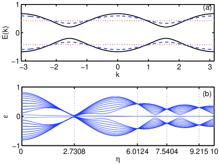
Figure 1: (color online) (a) Dispersion curves of the effective time-averaged Hamiltonian (III) [directly obtained from Eq. (III)] for $\chi=2.408$, and three different modulational Zeeman field parameters: $\eta=5$ (black solid line), $\eta=5.5$ (blue dashed line), and $\eta=6.0124$ (red dotted line). Other parameters are fixed as $m=2,\chi=2.408,\nu=1,\alpha=0.4\pi$. (b) Numerically-computed quasi-energy spectrum of the original time-periodic TB model (1) (with a chain of $21$ sites) as a function of the normalized modulation amplitude of Zeeman field $\eta$. $\Omega_{0}=2\omega=40$, and the other parameters are the same as in panel (a).

Now we move on to seek for the parameter condition under which the band flatness exists as presented in Fig. 1(a). In order to fully suppress the usual inter-site tunneling in the absence of SO coupling ($\alpha=0$), we should first fix the optical lattice shaking parameter $\chi=\bar{\xi}$ as a zero of the Bessel function $J_{0}$, which means vanishing of the effective spin-conserving hopping between nearest-neighboring sites, say, $\nu J_{0}(\chi)\cos\alpha=0$. Under such a circumstance, the lower and upper dispersion bands are symmetric with respect to $E=0$, and the dependence of $E_{\pm}(k)$ on the wave vector $k$ is fully governed by the Zeeman field parameter $\eta$ through the factor $J_{-m}^{+}J_{-m}^{-}$ in Eq. (III).

For the nonzero SO coupling case, it is readily concluded from Eq. (III) that under the prerequisite condition $J_{0}(\chi)=0$, the band flatness can be achieved when one of the equations: $J_{-m}^{\pm}\equiv J_{-m}(\eta\pm\bar{\xi})=0$ is satisfied, which occurs provided that $\eta$ is taken as

$$\eta_{l}^{\pm}=\beta_{l}\pm\bar{\xi},$$ (11)

with $\beta_{l}(~{}l=1,2,\dots)$ standing for the $l$th zero of $J_{-m}$ (i.e., $J_{-m}(\beta_{l})=0$).

Thus, flat bands in $k$-space are achieved with the energy dispersion given by the simple form

$$E_{\pm}=\pm|\nu\sin\alpha||J_{-m}^{\pm}(\eta_{l}^{\pm})|.$$ (12)

From Eq. (12), it is clear that in the presence of SO coupling ($\sin\alpha\neq 0$), there is always an energy gap between the two flat bands, while in the absence of SO coupling ($\sin\alpha=0$), the energy gap closes as $E_{\pm}=0$. This marks that the SO coupling parameter has nontrivial contribution to the characteristic of flat bands.

As an illustration with $\Omega_{0}=2\omega$ (i.e., $m=2$), we take $\chi=\bar{\xi}=2.408$ (the first zero of $J_{0}$), from Eq. (11) it follows that the band flatness occurs for the sequence of $\eta$ values listed in increasing order as $\{\eta_{1}^{-}=\beta_{1}-\bar{\xi},\eta_{2}^{-}=\beta_{2}-\bar{\xi},\eta_{1}^{+}=\beta_{1}+\bar{\xi},\eta_{3}^{-}=\beta_{3}-\bar{\xi},...\}$ with $\beta_{l}(~{}l=1,2,\dots)$ satisfying $J_{-2}(\beta_{l})=0$. The flatband physics can be understood by exploring the effective velocity of the atomic wave packet, which is defined by the variance of dispersion with respect to the wave vector, $v_{\rm{eff}}=dE(k)/dk$. Such an extreme band flattening, $v_{\rm{eff}}=dE(k)/dk=0$, implies that the dispersive propagation is fully suppressed and DL occurs.

So far our study is limited to the analytic arguments starting from the time-averaged Hamiltonian (III). To validate the results obtained with the effective time-averaging approach, we plot the numerically-computed quasienergy spectrum of the original time-periodic model (1) versus the dimensionless parameter $\eta$ in a finite lattice comprising $N=21$ sites for $\Omega_{0}=2\omega=40,\chi=2.408,\nu=1,\alpha=0.4\pi$. Throughout this paper, numerical simulations on the tight-binding model (1) are performed with open boundary conditions. As illustrated in Fig. 1 (b), the quasienergies make up two separated bands and exhibit a series of band collapses at which the quasienergies shrink into two distinct degenerate points at the values exactly predicted by Eq. (12). These collapses occur at $\eta=2.7308,6.0124,7.5404,9.2150,...$, which is exactly in correspondence with the sequence of $\eta$ values (hereafter we call these $\eta$ values as DL points) given by Eq. (11). Note that the degenerate quasienergies at these DL points correspond to the energies of the time-averaged system for different values of $k$ distributed over the whole Brillouin zone $k\in[-\pi,\pi]$. As compared with the energy curves plotted in $k$-space, the quasienergy spectrum as illustrated in Fig. 1 (b), due to finite-size effects, shows a pair of additional quasienergies oscillating weakly about zero, which split off from the two separated bands and physically correspond to two edge states.

Let us now investigate what unconventional features SO coupling brings to the dynamics at the DL points. Two distinct cases for this problem are listed as follows.

III.1 Case I

When $J_{0}(\chi)=0$ and $J_{-m}^{+}=0$, from Eq. (III), we have the effective Hamiltonian,

$$\hat{H}_{\rm{eff}}= \nu J_{-m}^{-}\sin\alpha\sum_{n}(\hat{c}_{n}^{{\dagger}}\hat{\sigma}_{+}\hat{c}_{n+1}+h.c.)$$

$$= \nu J_{-m}^{-}\sin\alpha\sum_{n}(\hat{c}_{n,\uparrow}^{{\dagger}}\hat{c}_{n+1,\downarrow}+h.c.).$$ (13)

In the Hilbert space expanded by the Wannier state basis $\{|n,\sigma\rangle\}$, i.e., $\{\cdots,|0,\downarrow\rangle,|0,\uparrow\rangle,|1,\downarrow\rangle,|1,\uparrow\rangle,\cdots\}$, $\hat{H}_{\rm{eff}}$ becomes a block diagonal matrix

$$\hat{H}_{\rm{eff}}=\left(\begin{array}[]{cccc}H_{two-state}^{I}&0&\cdots&0\\ 0&H_{two-state}^{I}&\cdots&0\\ \vdots&\vdots&\ddots&\vdots\\ 0&0&\cdots&H_{two-state}^{I}\\ \end{array}\right).$$ (14)

Here $H_{two-state}^{I}$ represents the $2\times 2$ block submatrix in the subspace spanned by only two states $|n,\uparrow\rangle,~{}|n+1,\downarrow\rangle$, i.e.,

$$H_{two-state}^{I}=\left(\begin{array}[]{cc}0&\nu J_{-m}^{-}\sin\alpha\\ \nu J_{-m}^{-}\sin\alpha&0\\ \end{array}\right).$$ (15)

III.2 Case II

When $J_{0}(\chi)=0$ and $J_{-m}^{-}=0$, the effective Hamiltonian (III) becomes

$$\hat{H}_{\rm{eff}} =-\nu J_{-m}^{+}\sin\alpha\sum_{n}(\hat{c}_{n}^{{\dagger}}\hat{\sigma}_{-}\hat{c}_{n+1}+h.c.)$$

$$=-\nu J_{-m}^{+}\sin\alpha\sum_{n}(\hat{c}_{n,\downarrow}^{{\dagger}}\hat{c}_{n+1,\uparrow}+h.c.).$$ (16)

With the Wannier state basis $\{\cdots,|0,\uparrow\rangle,|0,\downarrow\rangle,|1,\uparrow\rangle,|1,\downarrow\rangle,\cdots\}$, $\hat{H}_{\rm{eff}}$ is also a block diagonal matrix whose diagonal contains blocks of $2\times 2$ submatrix $H_{two-state}^{II}$ in the subspace spanned by two states $|n,\uparrow\rangle,~{}|n-1,\downarrow\rangle$,

$$H_{two-state}^{II}=\left(\begin{array}[]{cc}0&-\nu J_{-m}^{+}\sin\alpha\\ -\nu J_{-m}^{+}\sin\alpha&0\\ \end{array}\right).$$ (17)

According to the above analysis, for the SO-coupled lattice system, DL means that the lattice divides into a chain of disconnected dimers. When DL occurs, a spin $\sigma$ atom tunnels back and forth either between the initially occupied site and its left neighboring site or between the initially occupied site and its right neighboring site, and spin flipping accompanies the tunneling process. The tunneling direction depends on which of two equations $J_{-m}^{\pm}=0$ is satisfied. As mentioned above, the DL (two-site oscillation) arises for the SO-coupled lattice system, which is intrinsically connected with the two-band flatness and qualitatively distinct from the scenario where the CDT (completely frozen dynamics of the particle) is expected for a particle hopping on a conventional lattice without SO coupling in the high-frequency regime $\omega>>v$ as considered in this work.

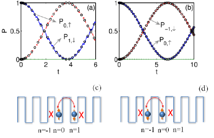
Figure 2: (color online) Time evolutions of the occupation probabilities, $P_{n,\sigma}(t)=\langle\psi|\hat{c}^{\dagger}_{n\sigma}\hat{c}_{n\sigma}|\psi\rangle=|c_{n,\sigma}(t)|^{2}$, in the original SO-coupled TB system (1) (with a chain of $N=21$ sites) for the system initially prepared in state $|0,\uparrow\rangle$. (a) $\chi=\bar{\xi}=2.408,\eta=\beta_{2}-\bar{\xi}=6.0124$; (b) $\chi=\bar{\xi}=2.408,\eta=\beta_{1}+\bar{\xi}=7.5404$. The other parameters are set as $\Omega_{0}=2\omega=40,\nu=1,\alpha=0.4\pi$. The open circles denote the analytical correspondences obtained from the two-state models (15) and (17). Lower panels (c) and (d) are schematic representations of the tunneling dynamics presented in panels (a) and (b) respectively. Red crosses indicate suppression of tunneling through that barrier, and the two-headed arrows indicate the allowed Rabi tunneling with spin flipping.

To illustrate the DL effect more clearly, without loss of generality, we start the system with a single spin-up atom at a certain site $n=j$, that is, the initial state given by $|\psi(0)\rangle=|j,\uparrow\rangle$. At the DL points where $J_{0}(\chi=\bar{\xi})=0$ and $J_{-m}^{+}\equiv J_{-m}(\eta+\bar{\xi})=0$ (i.e., $\eta=\beta_{l}-\bar{\xi}$), applying the initial condition to the two-state model (15) produces the analytical probabilities, $P_{j,\uparrow}=\cos^{2}(\omega_{1}^{\prime}t),P_{j+1,\downarrow}=\sin^{2}(\omega_{1}^{\prime}t)$, and $P_{n,\sigma}=0$ for $n\neq j,j+1$, with $\omega_{1}^{\prime}=|\nu J_{-m}^{-}\sin\alpha|=|\nu J_{-m}(\beta_{l}-2\bar{\xi})\sin\alpha|$ depending on the driving field and SO coupling parameter. Correspondingly, the Rabi period is given by $T_{1}=\pi/\omega_{1}^{\prime}$. Time evolutions of the atomic probabilities $P_{n,\sigma}(t)=\langle\psi|\hat{c}^{\dagger}_{n\sigma}\hat{c}_{n\sigma}|\psi\rangle=|c_{n,\sigma}(t)|^{2}$ based on the original Hamiltonian (1) are shown in Fig. 2(a) for the system initialized in the state $|0,\uparrow\rangle$, and with the system parameters $\Omega_{0}=2\omega=40,\chi=\bar{\xi}=2.408,\eta=\beta_{2}-\bar{\xi}=6.0124,\nu=1,\alpha=0.4\pi$. The open circles denote the analytical correspondences described by two-state model. The result means the occurrence of spin-flipping Rabi oscillation restricted inside a dimer as shown schematically in Fig. 2(c), in which only periodic oscillations are allowed between the state $|j,\uparrow\rangle$ (here, we take $j=0$ as an example) and the state $|j+1,\downarrow\rangle$. Similarly, when the other DL requirement $J_{0}(\chi)=0$ and $J_{-m}^{-}\equiv J_{-m}(\eta-\bar{\xi})=0$ (i.e., $\eta=\beta_{l}+\bar{\xi}$) is satisfied, from Eq. (17) with the initial condition $|\psi(0)\rangle=|j,\uparrow\rangle$, we derive the analytical probabilities $P_{j,\uparrow}=\cos^{2}(\omega_{2}^{\prime}t),P_{j-1,\downarrow}=\sin^{2}(\omega_{2}^{\prime}t)$, and $P_{n,\sigma}=0$ for $n\neq j,j+1$, with Rabi period $T_{2}=\pi/\omega_{2}^{\prime}$, $\omega_{2}^{\prime}=|\nu J_{-m}^{+}\sin\alpha|=|\nu J_{-m}(\beta_{l}+2\bar{\xi})\sin\alpha|$. The corresponding time evolutions of the occupation probabilities are plotted in Fig. 2(b) for the same initial condition and system parameters as in Fig. 2(a) and yet different $\eta=\beta_{1}+\bar{\xi}=7.5404$, where the numerical results (see the colored curves) from the full TB Hamiltonian (1) are in good agreement with the analytical ones (open circles). They describe spin-flipping Rabi oscillation along another pathway between the sites $n=j$ and $n=j-1$ as shown schematically in Fig. 2(d), where only periodic oscillations (see the two-headed arrow) are possible between the states $|j,\uparrow\rangle$ (here $j=0$) and $|j-1,\downarrow\rangle$. In the bottom schematic diagrams [panels (c) and (d)], the red crosses in the barriers indicate that the tunneling is not allowed and the two-headed arrows indicate that the Rabi tunneling with spin flipping is allowed.

Figure 3: (color online) The spatiotemporal evolutions of $P_{n,\uparrow}(t)=|c_{n,\uparrow}(t)|^{2}$ (left column) and $P_{n,\downarrow}=|c_{n,\downarrow}(t)|^{2}$ (right column), obtained from the original TB system (1) (with the size of $13$ sites) for a single spin-up atom initialized at site $n=0$, with the system parameters $\Omega_{0}=2\omega=40,\chi=\bar{\xi}=2.408,\nu=1,\alpha=0.4\pi$. The lighter areas correspond to the larger values of probability. As shown in the upper row [(a),(b)], the rightward directed motion with periodic spin-flipping is produced by repeating the changes between $\eta=\beta_{2}-\bar{\xi}=6.0124$ and $\eta=\beta_{1}+\bar{\xi}=7.5404$ at the times $t=n(T_{1}+T_{2})/2$ and $t=n(T_{1}+T_{2})/2+T_{2}/2$ for $n=0,1,2,...$; while as in the lower row [(c),(d)], interchanging the order of the modulation of the Zeeman field produces directed motion with periodic spin-flipping in the opposite direction.

As mentioned above, by means of a novel resonance effect between the static Zeeman field and the frequency of the driving field, we can realize the DL phenomenon where the single SO-coupled atom is restricted to making a standard two-site Rabi oscillation (complete population transfer) accompanied with spin flipping. In this case, tunneling is only permitted between two sites, and the initially localized atom with a given spin can make complete tunneling either to its left neighbor site or to its right neighbor site. The tunneling direction is determined by which of the two equations $\eta=\beta_{l}\pm\bar{\xi}$ is satisfied, where the plus in the plus-minus sign is associated with $J_{-m}^{-}\equiv J_{-m}(\eta-\bar{\xi})=0$ [leading to motion of a spin-up (spin-down) atom initially localized in a given site to the left (right), with the tunneling time $T_{2}/2=\pi/(2\omega_{2}^{\prime})$], and the minus sign corresponds to $J_{-m}^{+}\equiv J_{-m}(\eta+\bar{\xi})=0$ [leading to motion of a spin-up (spin-down) atom initially localized in a given site to the right (left), with the tunneling time $T_{1}/2=\pi/(2\omega_{1}^{\prime})$].

By make use of the new DL effects illustrated in Fig. 2, we can propose a scheme to realize ratchetlike motion of a single atom with spin flipping. The directed transport (DT) process is illustrated in Fig. 3, where $\Omega_{0}=2\omega=40,\chi=\bar{\xi}=2.408,\nu=1,\alpha=0.4\pi$. The spin-up particle is loaded into site $n=0$ and the parameters of the modulational Zeeman field are chosen as $\eta=\beta_{2}-\bar{\xi}=6.0124$ satisfying $J_{-m}^{+}\equiv J_{-m}(\eta+\bar{\xi})=0$ initially. The Rabi oscillation with spin flipping will occur between the initial site $n=0$ and its right neighbor site $n=1$, with Rabi period $T_{1}=\pi/\omega_{1}^{\prime}$. At $t=T_{1}/2$, the particle arrives at site $n=1$ with spin down. At this time, we immediately adjust the modulational Zeeman field as $\eta=\beta_{1}+\bar{\xi}=7.5404$ to fit $J_{-m}^{-}\equiv J_{-m}(\eta-\bar{\xi})=0$ such that the particle enters into a new spin-flipping Rabi oscillation between sites $n=1$ and $n=2$, with the Rabi period $T_{2}=\pi/\omega_{2}^{\prime}$. When a time interval of $T_{2}/2$ has elapsed, the particle has completely tunneled to site $n=2$ and the spin has been flipped back to up. At the moment, we tune the driving strength from $\eta=\beta_{1}+\bar{\xi}=7.5404$ to $\eta=\beta_{2}-\bar{\xi}=6.0124$; then the single particle will tunnel from site $n=2$ to site $n=3$ and spin will be again flipped from up to down. If we repeatedly change the $\eta$ values between $\eta=\beta_{2}-\bar{\xi}=6.0124$ and $\eta=\beta_{1}+\bar{\xi}=7.5404$ at the times $t=n(T_{1}+T_{2})/2$ and $t=n(T_{1}+T_{2})/2+T_{2}/2$ for $n=0,1,2,...$, the initial spin-up particle will propagate solely to the right, with spin flipped periodically in the transport process. The rightward DT is numerically confirmed from the original TB model (1), as shown in Figs. 3 (a) and (b), where the left (right) panel shows the spatiotemporal evolutions of the occupation probability of the spin-up (spin-down) component, $P_{n,\uparrow}$ ($P_{n,\downarrow}$), respectively. Conversely, if the order of the modulation is interchanged, the initial spin-up particle will propagate solely to the left as shown in Figs. 3 (c) and (d). The spatiotemporal evolutions of $P_{n,\uparrow}(t)=|c_{n,\uparrow}(t)|^{2}$ [Fig. 3 (c)] and $P_{n,\downarrow}=|c_{n,\downarrow}(t)|^{2}$ [Fig. 3 (d)] illustrate that the spin is flipped periodically in the leftward DT process. It is interesting to note that the direction of the particle’s propagation also depends on whether the initial spin is $\uparrow$ or $\downarrow$. Thus, we can control two reverse spin currents of the single atom, where a single SO-coupled atom can be transported toward opposite directions, by adjusting the modulational Zeeman field parameters at some appropriate operation times. We note that the directed motion was previously proposed by means of a distinct DL mechanism of the driven bipartite latticeCreffield2 , which nevertheless needs additional choice of the precise values of the SO coupling strengthHai1 .

The above investigation assumes that the lattice and Zeeman field oscillate in phase with the same frequency, viz. in Hamiltonian (1), $f(t)=f_{0}\cos(\omega t+\phi)$ and $\Omega(t)=\Omega_{0}+\Omega_{1}\cos(\omega t)$, where the phase difference $\phi$ between the two periodic drivings is set equal to zero. In order to gain more insight into the nature of the symmetry-breaking shown in Fig. 2, we will have a preliminary discussion about the effect of including a nonzero phase shift $\phi$ on the directed motion. With the same time-averaging procedure as in (4), the effective Hamiltonian for general $\phi$ is again given by Eq. (III), but with the substitutions

$$J_{-m}^{-}\rightarrow H_{1},~{}~{}~{}J_{-m}^{+}\rightarrow H_{2},$$ (18)

where we have defined

$$H_{1}=\sum_{k=-\infty}^{\infty}J_{k}(-\chi)J_{-m-k}(\eta)e^{ik\phi},~{}~{}~{}H_{2}=\sum_{k=-\infty}^{\infty}J_{k}(-\chi)J_{k-m}(\eta)e^{ik\phi}.$$ (19)

By use of the identities, $J_{m}(z_{1}+z_{2})=\sum_{k=-\infty}^{+\infty}J_{k}(z_{1})J_{m-k}(z_{2})$ and $J_{k}(-z)=(-1)^{k}J_{k}(z)=J_{-k}(z)$, we receive the following results for two specific cases: (i) When $\phi=0$, then $H_{1}=J_{-m}(\eta-\chi),~{}H_{2}=J_{-m}(\eta+\chi)$; and (ii) when $\phi=\pi$, then $H_{1}=J_{-m}(\eta+\chi),~{}H_{2}=J_{-m}(\eta-\chi)$. Evidently, in the former case, the results exactly recover the formulas in (III) and (6), but in the second case, the values of two effective spin-flipping-hopping amplitudes are just interchanged. For the other values of $\phi$ (namely, $\phi\neq 0,\pi$), $H_{1}$ and $H_{2}$ may be complex-valued. With the same modulational parameters as in Fig. 2 (a), $\chi=\bar{\xi}=2.408,\eta=\beta_{2}-\bar{\xi}=6.0124$, we readily derive the results for the above-mentioned two cases as follows: (i) At $\phi=0$, $H_{2}$ vanishes, but $H_{1}$ does not; (ii) at $\phi=\pi$, however, $H_{1}$ vanishes, but $H_{2}$ does not. This property implies that the direction of ratchetlike motion can be inverted by only changing the value of $\phi$ from $0$ to $\pi$.

One question naturally raised is: what breaks the left-right symmetry of the lattice, and why applying a phase shift of $\pi$ between the two drivings inverts the dimerization of the lattice. Here, we will provide a possibly simple explanation for the physical mechanism behind such a phenomenon. Suppose a spin $\uparrow$ atom tunnels from site $n$ to $n+1$ ($n-1$) via rightward (leftward) spin-flipping hopping, there will be a corresponding on-site energies change, $\tilde{B}_{1}(t)=V_{n,\uparrow}-V_{n+1,\downarrow}=\Omega(t)-f(t)$ [$\tilde{B}_{2}(t)=V_{n,\uparrow}-V_{n-1,\downarrow}=\Omega(t)+f(t)$] with $V_{n,\sigma}=\pm\Omega(t)/2+nf(t)$ ($+$ for $\sigma=\uparrow$, and $-$ for $\sigma=\downarrow$), respectively, in which the first part of energy change, $\Omega(t)$, comes from spin-flipping, and the second part $f(t)$ from lattice shaking. It behaves as if the rightward (leftward)-hopping atom moves feeling a combined periodically driving field $\tilde{B}_{1}(t)=\Omega(t)-f(t)$ [$\tilde{B}_{2}(t)=\Omega(t)+f(t)$] respectively. In this case, the driven SO-coupled system behaves approximately, in a time-averaged sense, like an undriven one, where the tunneling rate from state $|n,\uparrow\rangle$ to $|n+1,\downarrow\rangle$ is renormalized by a factor of $\frac{\omega}{2\pi}\int_{0}^{2\pi/\omega}dt\exp[-i\int_{0}^{t}dt^{\prime}\tilde{B}_{1}(t^{\prime})]$, and the tunneling rate from state $|n,\uparrow\rangle$ to $|n-1,\downarrow\rangle$ is renormalized instead by a factor of $\frac{\omega}{2\pi}\int_{0}^{2\pi/\omega}dt\exp[-i\int_{0}^{t}dt^{\prime}\tilde{B}_{2}(t^{\prime})]$. As we can see, the values of rescaled spin-flipping-tunneling rate are determined by configurations of the combined periodic fields $\tilde{B}_{1,2}(t)$ that the atom feels [strictly speaking, determined by $\pm\tilde{B}_{1,2}(t)$ for the reason that the Hermitian conjugate hopping term accounting for the reverse hopping process gives rises to the on-site energies change with opposite sign, namely, the effective tunneling rates occur in complex conjugate pairs]. In principle, owing to $\tilde{B}_{1}(t)\neq\pm\tilde{B}_{2}(t)$, the spin $\uparrow$ atom moving to its two neighbors with spin-flipping suffers from different combined periodic fields, and thus breaking of left-right symmetry is to be generically expected. When the phase difference $\phi=\pi$ is applied between the two drivings, the two combined periodic fields seen by the spin $\uparrow$ atom with spin-flipping tunneling toward two different directions are just swapped as compared with the case of the two in-phase drivings (i.e., $\phi=0$), thereby leading to inversion of the dimerization of the lattice. Overall, we might intuitively think that the breaking of left-right symmetry is a consequence of the combined effect of two drivings. A thorough investigation of the phase-controlled directed motion is worthy to be treated in a future work.

IV SO-coupling-related second-order tunneling and dynamical localization in far-off-resonant regime

In the preceding section, we only treat the resonant case. And then a question naturally follows: When the time-periodic modulation is not dealt with in the multiphoton resonance regime, does the phenomenon of suppression of quantum diffusion exist? If it does, what new physical features will be shown? In this section, we are trying to address these issues. We turn to the off-resonant case where the static Zeeman field $\Omega_{0}$ is not equal to any integer multiple of $\omega$, i.e., $\Omega_{0}\neq m\omega$ for any integer $m$ (absence of multiphoton resonances). Of particular interest is the far-off-resonant regime with $\Omega_{0}/\omega=u$ (here, by “far-off-resonant”, we mean that $u$ should take values sufficiently far from any integer) and $\omega\gg\nu$. In this far-off-resonant regime, the time-averaging treatment becomes invalid, and we will instead perform a multiple-scale asymptotic analysis Longhi2 ; Hai2 ; Luo3 of the spin-orbit-coupled bosonic system (II) under two in-phase drivings. To that end, we start by introducing the normalized time variable $\tau=\omega t$ and the small parameter $\epsilon=\nu/\omega$. Making the transformation $c_{n,\uparrow}=C_{n,\uparrow}e^{-i\frac{\sin(\omega t)}{\omega}(\frac{\Omega_{1}}{2}+f_{0}n)-i\frac{\Omega_{0}}{2}t},~{}c_{n,\downarrow}=C_{n,\downarrow}e^{-i\frac{\sin(\omega t)}{\omega}(-\frac{\Omega_{1}}{2}+f_{0}n)+i\frac{\Omega_{0}}{2}t}$, and recalling that $\chi=f_{0}/\omega$ and $\eta=\Omega_{1}/\omega$, we rewrite Eq. (II) in terms of the new amplitudes $C_{n,\sigma}$ as follows

$$i\frac{dC_{n,\uparrow}}{d\tau}= -\epsilon\cos\alpha\left(e^{-i\chi\sin\tau}C_{n+1,\uparrow}+e^{i\chi\sin\tau}C_{n-1,\uparrow}\right)$$

$$+\epsilon\sin\alpha\left(e^{-i(\chi-\eta)\sin\tau+iu\tau}C_{n+1,\downarrow}-e^{i(\chi+\eta)\sin\tau+iu\tau}C_{n-1,\downarrow}\right)$$

$$i\frac{dC_{n,\downarrow}}{d\tau}= -\epsilon\cos\alpha\left(e^{-i\chi\sin\tau}C_{n+1,\downarrow}+e^{i\chi\sin\tau}C_{n-1,\downarrow}\right)$$

$$-\epsilon\sin\alpha\left(e^{-i(\chi+\eta)\sin\tau-iu\tau}C_{n+1,\uparrow}-e^{i(\chi-\eta)\sin\tau-iu\tau}C_{n-1,\uparrow}\right).$$ (20)

We seek for a solution to Eq. (IV) as a power-series expansion in the smallness parameter $\epsilon$:

$$C_{n,\uparrow}= C_{n,\uparrow}^{(0)}+\epsilon C_{n,\uparrow}^{(1)}+\epsilon^{2}C_{n,\uparrow}^{(2)}+\cdots,$$

$$C_{n,\downarrow}= C_{n,\downarrow}^{(0)}+\epsilon C_{n,\downarrow}^{(1)}+\epsilon^{2}C_{n,\downarrow}^{(2)}+\cdots.$$ (21)

At the same time, we introduce multiple scales for time, $\tau_{0}=\tau,~{}\tau_{1}=\epsilon\tau,~{}\tau_{2}=\epsilon^{2}\tau,\dots$, and then replace the time derivatives by the expansion

$$\frac{d}{d\tau}=\partial_{\tau_{0}}+\epsilon\partial_{\tau_{1}}+\epsilon^{2}\partial_{\tau_{2}}+\cdots.$$ (22)

Substituting Eqs. (IV) and (22) into Eq. (IV), we obtain a hierarchy of equations for successive corrections to $C_{n,\uparrow},~{}C_{n,\downarrow}$ at different orders in $\epsilon$. At the leading order $\epsilon^{0}$, we find

$$i\frac{dC_{n,\uparrow}^{(0)}}{d\tau_{0}}=0, ~{}~{}C_{n,\uparrow}^{(0)}=A_{n,\uparrow}(\tau_{1},\tau_{2},\cdots),$$

$$i\frac{dC_{n,\downarrow}^{(0)}}{d\tau_{0}}=0, ~{}~{}C_{n,\downarrow}^{(0)}=A_{n,\downarrow}(\tau_{1},\tau_{2},\cdots),$$ (23)

where the amplitudes $A_{n,\uparrow}(\tau_{1},\tau_{2},\cdots)$ and $A_{n,\downarrow}(\tau_{1},\tau_{2},\cdots)$ are functions of the slow time variables $\tau_{1},\tau_{2},\cdots$, but independent of the fast time variable $\tau_{0}$. At order $\epsilon^{1}$ we have

$$i\frac{\partial C_{n,\uparrow}^{(1)}}{\partial\tau_{0}}= -i\partial_{\tau_{1}}A_{n,\uparrow}-\cos\alpha\left(e^{-i\chi\sin\tau}A_{n+1,\uparrow}+e^{i\chi\sin\tau}A_{n-1,\uparrow}\right)$$

$$+\sin\alpha\left(e^{-i(\chi-\eta)\sin\tau+iu\tau}A_{n+1,\downarrow}-e^{i(\chi+\eta)\sin\tau+iu\tau}A_{n-1,\downarrow}\right),$$

$$i\frac{\partial C_{n,\downarrow}^{(1)}}{\partial\tau_{0}}= -i\partial_{\tau_{1}}A_{n,\downarrow}-\cos\alpha\left(e^{-i\chi\sin\tau}A_{n+1,\downarrow}+e^{i\chi\sin\tau}A_{n-1,\downarrow}\right)$$

$$-\sin\alpha\left(e^{-i(\chi+\eta)\sin\tau-iu\tau}A_{n+1,\uparrow}-e^{i(\chi-\eta)\sin\tau-iu\tau}A_{n-1,\uparrow}\right).$$ (24)

For the convenience of our discussion, we rewrite the above equation (IV) as

$$i\frac{\partial C_{n,\uparrow}^{(1)}}{\partial\tau_{0}}= -i\partial_{\tau_{1}}A_{n,\uparrow}+K_{n}^{(1)}(\tau_{0}),$$

$$i\frac{\partial C_{n,\downarrow}^{(1)}}{\partial\tau_{0}}= -i\partial_{\tau_{1}}A_{n,\downarrow}+M_{n}^{(1)}(\tau_{0}).$$ (25)

To avoid the occurrence of secularly growing terms in the solutions $C_{n,\uparrow}^{(1)}$ and $C_{n,\downarrow}^{(1)}$, the solvability conditions

$$i\partial_{\tau_{1}}A_{n,\uparrow}=\overline{K_{n}^{(1)}(\tau_{0})},~{}~{}i\partial_{\tau_{1}}A_{n,\downarrow}=\overline{M_{n}^{(1)}(\tau_{0})}$$ (26)

must be satisfied. Throughout our paper, the overline denotes the time average with respect to the fast time variable $\tau_{0}$. The solvability condition at order $\epsilon^{1}$ [Eq. (26)] then gives

$$i\partial_{\tau_{1}}A_{n,\uparrow}= -\cos\alpha J_{0}(\chi)(A_{n+1,\uparrow}+A_{n-1,\uparrow}),$$

$$i\partial_{\tau_{1}}A_{n,\downarrow}= -\cos\alpha J_{0}(\chi)(A_{n+1,\downarrow}+A_{n-1,\downarrow}).$$ (27)

According to $C_{n,\uparrow}^{(1)}=-i\int[K_{n}^{(1)}(\tau_{0})-\overline{K_{n}^{(1)}(\tau_{0})}]d\tau_{0}$ and $C_{n,\downarrow}^{(1)}=-i\int[M_{n}^{(1)}(\tau_{0})-\overline{M_{n}^{(1)}(\tau_{0})}]d\tau_{0}$, the amplitudes $C_{n,\uparrow},~{}C_{n,\downarrow}$ at order $\epsilon$ are given by

$$C_{n,\uparrow}^{(1)}= -\cos\alpha F_{0}(\tau_{0})A_{n+1,\uparrow}+\cos\alpha F_{0}^{*}(\tau_{0})A_{n-1,\uparrow}$$

$$-\sin\alpha F_{1}(\tau_{0})A_{n+1,\downarrow}+\sin\alpha F_{2}(\tau_{0})A_{n-1,\downarrow},$$

$$C_{n,\downarrow}^{(1)}= -\cos\alpha F_{0}(\tau_{0})A_{n+1,\downarrow}+\cos\alpha F_{0}^{*}(\tau_{0})A_{n-1,\downarrow}$$

$$-\sin\alpha F_{2}^{*}(\tau_{0})A_{n+1,\uparrow}+\sin\alpha F_{1}^{*}(\tau_{0})A_{n-1,\uparrow},$$ (28)

where

$$F_{0}(\tau_{0})= \sum_{\begin{subarray}{c}p=-\infty\\ p\neq 0\end{subarray}}^{\infty}\frac{J_{p}(\chi)e^{-ip\tau_{0}}}{p},$$

$$F_{1}(\tau_{0})= \sum_{p=-\infty}^{\infty}\frac{J_{p}(\chi-\eta)e^{i(-p+u)\tau_{0}}}{-p+u},$$

$$F_{2}(\tau_{0})= \sum_{p=-\infty}^{\infty}\frac{J_{p}(\chi+\eta)e^{i(p+u)\tau_{0}}}{p+u}.$$ (29)

At the next order $\epsilon^{2}$, we have

$$i\frac{\partial C_{n,\uparrow}^{(2)}}{\partial\tau_{0}}= -i\partial_{\tau_{2}}A_{n,\uparrow}-i\partial_{\tau_{1}}C_{n,\uparrow}^{(1)}+K_{n}^{(2)}(\tau_{0}),$$

$$i\frac{\partial C_{n,\downarrow}^{(2)}}{\partial\tau_{0}}= -i\partial_{\tau_{2}}A_{n,\downarrow}-i\partial_{\tau_{1}}C_{n,\downarrow}^{(1)}+M_{n}^{(2)}(\tau_{0}),$$ (30)

with

$$K_{n}^{(2)}(\tau_{0})= -\cos\alpha\left(e^{-i\chi\sin\tau}C_{n+1,\uparrow}^{(1)}+e^{i\chi\sin\tau}C_{n-1,\uparrow}^{(1)}\right)$$

$$+\sin\alpha\left(e^{-i(\chi-\eta)\sin\tau+iu\tau}C_{n+1,\downarrow}^{(1)}-e^{i(\chi+\eta)\sin\tau+iu\tau}C_{n-1,\downarrow}^{(1)}\right),$$

$$M_{n}^{(2)}(\tau_{0})= -\cos\alpha\left(e^{-i\chi\sin\tau}C_{n+1,\downarrow}^{(1)}+e^{i\chi\sin\tau}C_{n-1,\downarrow}^{(1)}\right)$$

$$-\sin\alpha\left(e^{-i(\chi+\eta)\sin\tau-iu\tau}C_{n+1,\uparrow}^{(1)}-e^{i(\chi-\eta)\sin\tau-iu\tau}C_{n-1,\uparrow}^{(1)}\right).$$

In order to avoid the occurrence of secularly growing terms in the solutions $C_{n,\uparrow}^{(2)}$ and $C_{n,\downarrow}^{(2)}$, the following solvability conditions must be satisfied:

$$i\partial_{\tau_{2}}A_{n,\uparrow}= \overline{K_{n}^{(2)}(\tau_{0})}$$

$$=-T\sin^{2}\alpha(A_{n+2,\uparrow}+A_{n-2,\uparrow})+\sin^{2}\alpha(E_{1}+E_{2})A_{n,\uparrow},$$

$$i\partial_{\tau_{2}}A_{n,\downarrow}= \overline{M_{n}^{(2)}(\tau_{0})}$$

$$=T\sin^{2}\alpha(A_{n+2,\downarrow}+A_{n-2,\downarrow})-\sin^{2}\alpha(E_{1}+E_{2})A_{n,\downarrow},$$ (31)

where we have set

$$T\equiv T(\eta,\chi,u)=\sum_{p=-\infty}^{\infty}\frac{J_{p}(\chi+\eta)J_{-p}(\chi-\eta)}{p+u},$$

$$E_{1}= \sum_{p=-\infty}^{\infty}\frac{J_{p}^{2}(\chi-\eta)}{-p+u},$$

$$E_{2}= \sum_{p=-\infty}^{\infty}\frac{J_{p}^{2}(\chi+\eta)}{p+u}.$$ (32)

Thus the evolution of the zeroth-order amplitudes $A_{n,\sigma}$ up to the second-order long time scale is given by

$$i\frac{dA_{n,\sigma}}{d\tau}=i\frac{\partial A_{n,\sigma}}{\partial\tau_{0}}+i\epsilon\frac{\partial A_{n,\sigma}}{\partial\tau_{1}}+i\epsilon^{2}\frac{\partial A_{n,\sigma}}{\partial\tau_{2}}.$$ (33)

Substituting Eqs. (IV), (IV) and (IV) into Eq. (33), and returning to the original time variable $t$, we obtain

$$i\frac{dA_{n,\uparrow}}{dt}= -\nu\cos\alpha J_{0}(\chi)(A_{n+1,\uparrow}+A_{n-1,\uparrow})+\frac{\nu^{2}\sin^{2}\alpha}{\omega}(E_{1}+E_{2})A_{n,\uparrow}$$

$$-\frac{\nu^{2}\sin^{2}\alpha}{\omega}T(A_{n+2,\uparrow}+A_{n-2,\uparrow}),$$

$$i\frac{dA_{n,\downarrow}}{dt}= -\nu\cos\alpha J_{0}(\chi)(A_{n+1,\downarrow}+A_{n-1,\downarrow})-\frac{\nu^{2}\sin^{2}\alpha}{\omega}(E_{1}+E_{2})A_{n,\downarrow}$$

$$+\frac{\nu^{2}\sin^{2}\alpha}{\omega}T(A_{n+2,\downarrow}+A_{n-2,\downarrow}).$$ (34)

Eq. (IV) correctly describes the dynamics of the original system (II) up to second-order time scale for the far-off-resonant case, where the coefficient $\nu^{2}\sin^{2}\alpha T/\omega$ describes the second-order tunneling rate between two next-nearest-neighboring sites. By neglecting the high-order terms [see Eq. (IV)], we can approximately view the probability amplitudes $C_{n,\sigma}$ as the zeroth order $C_{n,\sigma}=C_{n,\sigma}^{0}=A_{n,\sigma}$. Thus, $|A_{n,\sigma}|^{2}$ refers to the probability of finding a single particle with spin $\sigma$ at site $n$. As can be seen from Eq. (IV), the dynamics of spin $\uparrow$ is decoupled from that of spin $\downarrow$, and they are similar to the case of spinless atom. It is also clearly seen that in absence of SO coupling ($\sin\alpha=0$), it would be sufficient to fully suppress the tunneling in the system by taking $\chi$ as a zero of the Bessel function $J_{0}$, while in the presence of SO coupling, second-order tunneling remains possible through the SO-coupling-related term $\sin\alpha$ in Eq. (IV).

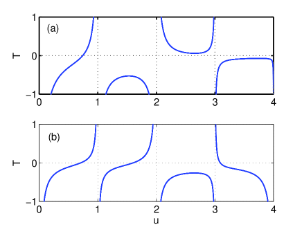
Figure 4: (color online) The factor $T$, defined by Eq. (IV), as a function of $u$, with fixed $\eta=1$, for (a) $\chi=2.4048$, and (b) $\chi=5.5201$.

Thus, it can be concluded that the frozen dynamics (more properly referred to as CDT) is attained when the two conditions

$$J_{0}(\chi)=0,~{}~{}~{}T(\eta,\chi,u)=0,$$ (35)

are simultaneously satisfied. Notice that the former requirement, $J_{0}(\chi)=0$, corresponds to the usual CDT condition in the high-frequency limit, while the latter represents suppression of second-order process arising from SO coupling. The numerical calculation shows that $T(\eta,\chi,u)$ can vanish, together with $J_{0}(\chi)$, for some values of parameters $\eta,\chi,u$. This is clearly shown in Figs. 4 (a) and (b), which describe the factor $T$ of the second-order tunneling coefficients as a function of the static Zeeman field parameter $u$ with fixed $\eta=1$, for $\chi=2.4048$ and $\chi=5.5201$ (the lowest two zeros of the $J_{0}$ Bessel function) respectively. In these plots, $T(\eta,\chi,u)$ is infinite whenever $u$ takes integer values (and is very large whenever $u$ is close to an integer). As a detailed inspection of the behavior of $T(\eta,\chi,u)$, we find that in the range $u\in(0,4)$, $T$ has only one zero point at $u=0.7414$ for $\chi=2.4048$ (i.e., one has $T=0$ with the parameters $\chi=2.4048,\eta=1,u=0.7414$), while $T$ has three zero points at $u=0.7076,1.6034,3.0924$ for $\chi=5.5201$ (at these points, the factor $T$ vanishes). Note that simultaneous vanishing of $J_{0}(\chi)$ and $T(\eta,\chi,u)$ means complete suppression of tunneling and hence existence of CDT phenomenon. In the above numerical calculations of $T(\eta,\chi,u)$, the cut-off value of $p$ is given by $p_{min}=-20$ and $p_{max}=20$, since the sums converge rapidly and the results remain unchanged if we include the terms of orders higher than the cut-off.

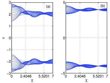
Figure 5: (color online) Numerically-computed quasienergies $\varepsilon$ of the time-periodic TB system (1) comprising $21$ sites as a function of the normalized parameters $\chi$. (a) $\eta=1,u=0.2$; (b) $\eta=1,u=1.6034$. The other parameters are $\omega=20,\nu=1,\alpha=0.4\pi$.

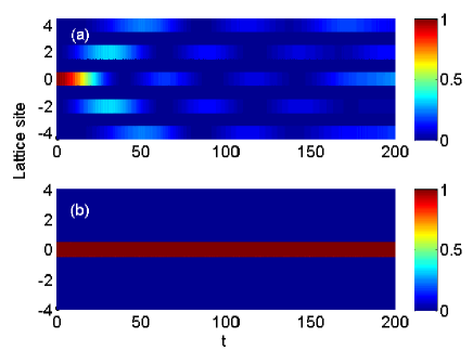
Figure 6: (color online) Spatiotemporal evolutions of the probability $P_{n,\uparrow}$ of the original TB system (1) for a spin-up atom initially localized at site $n=0$. (a) $\eta=1,u=0.2,\chi=5.5201$; (b) $\eta=1,u=1.6034,\chi=5.5201$. The other parameters are $\omega=20,\nu=1,\alpha=0.4\pi$. The corresponding occupation probabilities of spin-down component $P_{n,\downarrow}(t)$ are always negligible during the dynamical evolution and they are not displayed here.

To confirm the predictions of our asymptotic analysis, we have numerically calculated the quasienergy spectrum of the time-periodic TB system (1) versus the normalized parameter $\chi$ in a finite lattice with $21$ sites for $\eta=1$ and for two distinct values of $u=0.2$ [Fig. 5 (a)] and $u=1.6034$ [Fig. 5 (b)]. The other parameters are set as $\omega=20,\nu=1,\alpha=0.4\pi$. Comparing Fig. 5 (a) with Fig. 5 (b), we can observe a perfect collapse of quasi-energy bands only at the values of $u=1.6034,\chi=5.5201$ which precisely correspond to the second zero of $T(u)$ as shown in Fig. 4 (d). Our results for the spatiotemporal evolutions of the occupation probabilities of spin-up component $P_{n,\uparrow}(t)$ are also exemplified in Figs. 6 (a) and (b), by numerical analysis of original TB model (1) with the system parameters as discussed above. The corresponding occupation probabilities of spin-down component $P_{n,\downarrow}(t)$ (not displayed here) are always negligible during the dynamical evolution, due to the fact the usual inter-site hopping is basically suppressed because of $J_{0}(\chi=5.5201)=0$. As shown in Fig. 6 (a), where $\eta=1,u=0.2,\chi=5.5201$ [$T\neq 0$ and no collapse of quasi-energy bands exists, see Fig. 5 (a)], the spin-up atom initialized in site $n=0$ exhibits interesting spatially delocalized propagation. In contrast to usual dynamical tunneling, as is clearly shown in Fig. 6 (a), the initial spin-up atom can be directly transported to its next-nearest-neighboring sites without spin-flipping, which is well consistent with the predictions given by our asymptotic analysis. The non-spin-flipping tunneling between next-nearest-neighboring sites is a second-order tunneling process, which is a peculiar feature stemming from the SO coupling. Although the validity of asymptotic analysis requires that $u$ should be sufficiently far from any integer value, the full-numerical result as presented in Fig. 6 (a) shows that even at $u=0.2$ (being not very far away from the integer $0$), the asymptotic analysis is still a good approximation. This provides some convenience for directly transporting a spin to its non-nearest-neighboring sites without spin flipping. Conversely, when $\eta=1,u=1.6034,\chi=5.5201$ (at which the second-order tunneling factor $T$ vanishes and collapse of quasienergy bands exists), the spin-up atom remains frozen in its initially occupied site $n=0$ and CDT occurs as illustrated in Fig. 6 (b).

Before concluding, we further identify what parameter ranges of the quantity $u$ can be considered as far-off-resonant regimes where the results based on the multiple-scale asymptotic analysis are applicable. To that end, we define a related variable $\langle S\rangle=\frac{1}{\Delta t}\int_{0}^{\Delta t}dt\sum_{n^{\prime}}|c_{2n^{\prime},\uparrow}|^{2}$ with a long-enough averaging time interval $\Delta t$, which is used to measure the time-averaged total probability of finding the spin $\uparrow$ atom at all the $2n^{\prime}$ sites with integers $n^{\prime}=0,\pm 1,...$. On the condition that the usual spin-conserving tunneling is shut off by taking $J_{0}(\chi)=0$, and when the system is initialized in state $|0,\uparrow\rangle$, $\langle S\rangle=1$ means that the tunnelings (including the spin-flipping tunneling) between nearest-neighboring sites disappear which justifies the validity of the multiple-time-scale asymptotic analysis. As we know, the basic result based on the multiple-time-scale asymptotic analysis is that the spin-flipping tunneling between nearest-neighboring sites is impossible for any value of system parameters. Starting the system with a spin $\uparrow$ atom at site 0, from TB model (1) with size of 13 sites, we numerically give $\langle S\rangle$ as the function of $u$ for the other parameters as same as in Fig. 6. It is shown in Fig. 7 that the numerical results of $\langle S\rangle$ exhibit different features, as we vary the quantity $u$ to pass through the multiphoton resonant points, the near-resonant regions, and the far-off-resonant regions. At each of the resonant points ($\Omega_{0}=m\omega$ with integers $m$), $\langle S\rangle$ drops to the lowest levels, which indicates the largest nearest-neighbor-tunneling probabilities. As increasing $u$ to be the furthest from resonance (i.e., half-integer values, for example, $m=0.5,1.5,2.5$), $\langle S\rangle$ tends to 1, which indicates disappearance of nearest-neighbor-tunneling as predicted by the multiple-scale asymptotic analysis. Note that in the near-resonant regions where $\langle S\rangle$ transits from the lowest to near the highest values, the multiple-scale asymptotic analysis is also invalid. From Fig. 7, we may estimate that the parameter ranges of $u$ with $\langle S\rangle\geq 0.98$ can be regarded as belonging to the far-off-resonant regime in this paper, since in these regimes the multiple-scale asymptotic analysis works effectively. As shown in Fig. 7, the numerical values of $\langle S\rangle$ for the two specific cases exemplified in Fig. 6 can be observed to be $\langle S\rangle\geq 0.98$, indicating that the multiple-scale asymptotic analysis is valid at the values of $u=0.2$ and $u=1.6034$. The word “far-off-resonance” is used here for the following two reasons: (i) When $u$ is the furthest from resonance, the multiple-scale asymptotic analysis works well without any doubt; and (ii) when $u$ is moderately (but sufficiently) far from resonance, the multiple-scale asymptotic analysis still works, which is distinguished from the near-resonant regimes.

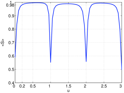
Figure 7: (color online) The quantity $\langle S\rangle$ as a function of $u$, with the system initialized in state $|0,\uparrow\rangle$. Here, $\langle S\rangle$ denotes the time-averaged total probability of finding the spin $\uparrow$ atom at all the $2n^{\prime}$ sites with integers $n^{\prime}=0,\pm 1,...$. The other system parameters are the same as in Fig. 6 (a): $\eta=1,\chi=5.5201,\omega=20,\nu=1,\alpha=0.4\pi$. The time used for averaging is 200 in dimensionless unit.

V conclusions

In summary, we have theoretically studied the tunneling dynamics of tight-binding model for a single SO-coupled atom trapped in a one-dimensional optical lattice, in the presence of a periodic time modulation of the Zeeman field and optical lattice shaking. By means of analytical and numerical methods, we have evidenced quasienergies flatness (collapse) and suppression of quantum diffusion for both multi-photon resonance and far-off-resonance cases. We have exposed a number of unconventional features of tunneling dynamics in the presence of SO coupling. For the resonant case, where the static Zeeman field matches an integer multiple of the driving frequency, we find that as DL occurs the system is divided into a chain of disconnected dimers, each of which is a two-state model that merely couples opposite spins at two neighboring sites. There exists no static bias inside each two-state model due to the removal of the static Zeeman field by the multi-photon resonance effect. In this case the particle is unable to diffuse over the lattice (evidence of DL phenomenon), and is restricted to performing a perfect two-site Rabi oscillation (the complete population transfer from one site of the dimer to the other) accompanied by spin flipping under the action of SO coupling. By using the two-site Rabi oscillation of the DL effect that are absent in conventional lattice system, we are able to generate a ratchetlike (directed) motion with periodic spin-flipping of the single SO-coupled atom, in which the direction of motion can be manipulated in a controllable way. For the far-off-resonant case, by means of the multiple-time-scale asymptotic analysis, we have revealed that besides the usual non-spin-flipping tunneling between nearest-neighboring sites, there exists a type of second-order tunneling between next-nearest-neighboring sites induced by the presence of SO coupling. It has been shown that suppression of the usual inter-site tunneling by lattice shaking is not enough to observe completely frozen dynamics (CDT), and suppression of the second-order tunneling via the Zeeman field modulation is also required.

Finally, we brief discuss the experimental aspects of our results. As implemented in the seminal worklin471 , a synthetic SO coupling can be realized by applying a pair of counterpropagating Raman beams to couple two hyperfine spin states $|\uparrow\rangle=|F=1,m_{F}=0\rangle$ and $|\downarrow\rangle=|F=1,m_{F}=-1\rangle$ (with the state $|F=1,m_{F}=1\rangle$ far detuned from this pseudo-spinor set) of a single ultracold atom. An appropriate optical lattice can be induced by two additional contrapropagating laser beams at $\lambda_{L}=1030$ nm wavelengthEckardt , with potential strength of the order $\sim 10E_{\textrm{rec}}$ [where $E_{\textrm{rec}}=2\hbar^{2}\pi^{2}/(m\lambda_{L}^{2})$], which guarantees the effectiveness of the tight-binding model. One can use an acousto-optic modulator to precisely control the lattice beam intensity, and to introduce a frequency difference between the beams that allows us to periodically shake the latticeEckardt . In addition, the Zeeman-field intensity can be tuned independently by the bias magnetic field and the frequency difference between the two Raman laser beams that couple the two internal atomic stateslin471 . Alternatively, the SO coupling considered in this work could be realized using the tripod scheme implemented with three laser beamsEdmonds . Based on these experiment setups mentioned above, it should be possible to test our results and in particular the new aspects of DL phenomenon induced by SO coupling.

- (1) M. Grifoni and P. Hänggi, Phys. Rep. 304, 229 (1998).
- (2) M. Bukov, L. D’Alessio, and A. Polkovnikov, Adv. Phys. 64, 139 (2015).
- (3) A. Eckardt, Rev. Mod. Phys. 89, 011004 (2017).
- (4) M. P. Silveri, J. A. Tuorila, E. V. Thuneberg, and G. S. Paraoanu, Rep. Prog. Phys. 80, 056002 (2017).
- (5) D. H. Dunlap and V. M. Kenkre, Phys. Rev. B 34, 3625 (1986).
- (6) M. Holthaus, Phys. Rev. Lett. 69, 351 (1992).
- (7) F. Grossmann, T. Dittrich, P. Jung, and P. Hanggi, Phys. Rev. Lett. 67, 516 (1991); Z. Phys. B 84, 315 (1991).
- (8) S. S. Hegde, H. Katiyar, T. S. Mahesh, and A. Das, Phys. Rev. B 90, 174407 (2014).
- (9) S. Longhi, M. Marangoni, M. Lobino, R. Ramponi, P. Laporta, E. Cianci, and V. Foglietti, Phys. Rev. Lett. 96, 243901 (2006).
- (10) R. Iyer, J. S. Aitchison, J. Wan, M. M. Dignam, and C. M. de Sterke, Opt. Express 15, 3212 (2007).
- (11) H. Lignier, C. Sias, D. Ciampini, Y. Singh, A. Zenesini, O. Morsch, and E. Arimondo, Phys. Rev. Lett. 99, 220403 (2007).
- (12) Y. K. Kato, R. C. Myers, A. C. Gossard, and D. D. Awschalom, Science 306, 1910 (2004).
- (13) B. A. Bernevig, T. L. Hughes, and S. C. Zhang, Science 314, 1757 (2006).
- (14) I. Z̆utić, J. Fabian, and S. Das Sarma, Rev. Mod. Phys. 76, 323 (2004).
- (15) D. Stepanenko and N. E. Bonesteel, Phys. Rev. Lett. 93, 140501 (2004).
- (16) Y. J. Lin, K. Jiménez-García, and I. B. Spielman, Nature (London) 471, 83 (2011).
- (17) P. J. Wang, Z. Q. Yu, Z. K. Fu, J. Miao, L. H. Huang, S. J. Chai, H. Zhai, and J. Zhang, Phys. Rev. Lett. 109, 095301 (2012).
- (18) L. W. Cheuk, A. T. Sommer, Z. Hadzibabic, T. Yefsah, W. S. Bakr, and M. W. Zwierlein, Phys. Rev. Lett. 109, 095302 (2012).
- (19) J. Zhang, S. Ji, Z. Chen, L. Zhang, Z. Du, B. Yan, G. Pan, B. Zhao, Y. Deng, H. Zhai, S. Chen, and J. Pan, Phys. Rev. Lett. 109, 115301 (2012).
- (20) L. Huang, Z. Meng, P. Wang, P. Peng, S. L. Zhang, L. Chen, D. Li, Q. Zhou, and J. Zhang, Nat. Phys. 12, 540 (2016).
- (21) Z. Wu, L. Zhang, W. Sun, X. T. Xu, B. Z. Wang, S. C. Ji, Y. Deng, S. Chen, X. J. Liu, and J. W. Pan, Science 354, 83 (2016).
- (22) Z. Cai, X. Zhou, and C. Wu, Phys. Rev. A 85, 061605(R) (2012).
- (23) W. S. Cole, S. Zhang, A. Paramekanti, and N. Trivedi, Phys. Rev. Lett. 109, 085302 (2012).
- (24) J. Radić, A. Di Ciolo, K. Sun, and V. Galitski, Phys. Rev. Lett. 109, 085303 (2012).
- (25) C. Hamner, Y. Zhang, M. A. Khamehchi, M. J. Davis, and P. Engels, Phys. Rev. Lett. 114, 070401 (2015).
- (26) Y. V. Kartashov, V. V. Konotop, D. A. Zezyulin, and L. Torner, Phys. Rev. Lett. 117, 215301 (2016).
- (27) Y. Zhang and C. Zhang, Phys. Rev. A 87, 023611 (2013).
- (28) L. Zhou, H. Pu, and W. Zhang, Phys. Rev. A 87, 023625 (2013).
- (29) K. Jiménez-García, L. J. LeBlanc, R. A. Williams, M. C. Beeler, C. Qu, M. Gong, C. Zhang, and I. B. Spielman, Phys. Rev. Lett. 114, 125301 (2015).
- (30) X. Luo, L. Wu, J. Chen, Q. Guan, K. Gao, Z. Xu, L. You, and R. Wang, Sci. Rep. 6, 18983 (2016).
- (31) S. Rahav, I. Gilary, and S. Fishman, Phys. Rev. A 68, 013820 (2003).
- (32) Y. Zhang, G. Chen, and C. Zhang, Sci. Rep. 3, 1937 (2013).
- (33) Z.-F. Xu, L. You, and M. Ueda, Phys. Rev. A 87, 063634 (2013).
- (34) Y. V. Kartashov, V. V. Konotop, and V. A. Vysloukh, Phys. Rev. A 97, 063609 (2018).
- (35) F. Kh. Abdullaev, M. Brtka, A. Gammal, and L. Tomio, Phys. Rev. A 97, 053611 (2018).
- (36) Y. Luo, G. Lu, C. Kong, and W. Hai, Phys. Rev. A 93, 043409 (2016).
- (37) X. Luo, B. Yang, J. Cui, Y. Guo, L. Li, and Q. Hu, J. Phys. B: At. Mol. Opt. Phys. 52, 085301 (2019).
- (38) Y. V. Kartashov, V. V. Konotop, D. A. Zezyulin, and L. Torner, Phys. Rev. A 94, 063606 (2016).
- (39) F. Kh. Abdullaev and M. Salerno, Phys. Rev. A 98, 053606 (2018).
- (40) M. Salerno, F. Kh. Abdullaev, A. Gammal, and L. Tomio, Phys. Rev. A 94, 043602 (2016).
- (41) D. V. Khomitsky, L. V. Gulyaev, and E. Ya. Sherman, Phys. Rev. B 85, 125312 (2012).
- (42) A. Eckardt, M. Holthaus, H. Lignier, A. Zenesini, D. Ciampini, O. Morsch, and E. Arimondo, Phys. Rev. A 79, 013611 (2009).
- (43) Z. Yu and J. Xue, Phys. Rev. A 90, 033618 (2014).
- (44) Y. Luo, X. Wang, Y. Luo, Z. Zhou, Z.-Y. Zeng, and X. Luo, New J. Phys. 22, 093041 (2020).
- (45) M. Glück, A. R. Kolovsky, and H. J. Korsch, Phys. Rep. 366, 103 (2002).
- (46) C. E. Creffield and T. S. Monteiro, Phys. Rev. Lett. 96, 210403 (2006).
- (47) C. E. Creffield, Phys. Rev. Lett. 99, 110501 (2007).
- (48) S. Longhi and V. G. Della, Phys. Rev. A 86, 042104 (2012).
- (49) Z. Zhou, W. Hai, Q. Xie, and J. Tan, New J. Phys. 15, 123020 (2013).
- (50) X. Luo, D. Wu, S. Luo, Y. Guo, X. Yu, and Q. Hu, J. Phys. A: Math. Theor. 47, 345301 (2014).
- (51) M. J. Edmonds, J. Otterbach, R. G. Unanyan, M. Fleischhauer, M. Titov, and P. Ohberg, New J. Phys. 14, 073056 (2012).