A multipoint stress-flux mixed finite element method for the Stokes-Biot model

Abstract

In this paper we present and analyze a fully-mixed formulation for the coupled problem arising in the interaction between a free fluid and a flow in a poroelastic medium. The flows are governed by the Stokes and Biot equations, respectively, and the transmission conditions are given by mass conservation, balance of stresses, and the Beavers-Joseph-Saffman law. We apply dual-mixed formulations in both domains, where the symmetry of the Stokes and poroelastic stress tensors is imposed by setting the vorticity and structure rotation tensors as auxiliary unknowns. In turn, since the transmission conditions become essential, they are imposed weakly, which is done by introducing the traces of the fluid velocity, structure velocity, and the poroelastic media pressure on the interface as the associated Lagrange multipliers. The existence and uniqueness of a solution are established for the continuous weak formulation, as well as a semidiscrete continuous-in-time formulation with non-matching grids, together with the corresponding stability bounds. In addition, we develop a new multipoint stress-flux mixed finite element method by involving the vertex quadrature rule, which allows for local elimination of the stresses, rotations, and Darcy fluxes. Well-posedness and error analysis with corresponding rates of convergence for the fully-discrete scheme are complemented by several numerical experiments.

1 Introduction

The interaction of a free fluid with a deformable porous medium, referred to as fluid-poroelastic structure interaction (FPSI), is a challenging multiphysics problem. It has applications to predicting and controlling processes arising in gas and oil extraction from naturally or hydraulically fractured reservoirs, modeling arterial flows, and designing industrial filters, to name a few. For this physical phenomenon, the free fluid region can be modeled by the Stokes (or Navier–Stokes) equations, while the flow through the deformable porous medium is modeled by the Biot system of poroelasticity. In the latter, the volumetric deformation of the elastic porous matrix is complemented with the Darcy equation that describes the average velocity of the fluid in the pores. The two regions are coupled via dynamic and kinematic interface conditions, including balance of forces, continuity of normal velocity, and a no slip or slip with friction tangential velocity condition. The model exhibits features of both coupled Stokes-Darcy flows and fluid-structure interaction (FSI).

To the authors’ knowledge, one of the first works in analyzing the Stokes-Biot coupled problem is [53], where well-posedness for the fully dynamic problem is established by developing an appropriate variational formulation and using semigroup methods. One of the first numerical studies is presented in [12], where monolithic and iterative partitioned methods are developed for the solution of the coupled system. A non-iterative operator splitting scheme with a non-mixed Darcy formulation is developed in [21]. Finite element methods for mixed Darcy formulations, where the continuity of normal flux condition becomes essential, are considered in [20] using Nitsche’s coupling and in [8] using a pressure Lagrange multiplier. More recently, a nonlinear quasi-static Stokes–Biot model for non-Newtonian fluids is studied in [3]. The authors establish well-posedness of the weak formulation in Banach space setting, along with stability and convergence of the finite element approximation. In [25], the fully dynamic coupled Navier-Stokes/Biot system with a pressure-based Darcy formulation is analyzed. Additional works include optimization-based decoupling method [24], a second order in time split scheme [44], various discretization methods [56, 13, 23], dimensionally reduced model for flow through fractures [22], and coupling with transport [4]. All of the above mentioned works are based on displacement formulations for the elasticity equation. In a recent work [47], the first mathematical and numerical study of a stress-displacement mixed elasticity formulation for the Stokes-Biot model is presented.

The goal of the present paper is to develop a new fully mixed formulation of the quasi-static Stokes-Biot model, which is based on dual mixed formulations for all three components - Darcy, elasticity, and Stokes. In particular, we use a velocity-pressure Darcy formulation, a weakly symmetric stress-displacement-rotation elasticity formulation, and a weakly symmetric stress-velocity-vorticity Stokes formulation. This formulation exhibits multiple advantages, including local conservation of mass for the Darcy fluid, local poroelastic and Stokes momentum conservation, and accurate approximations with continuous normal components across element edges or faces for the Darcy velocity, the poroelastic stress, and the free fluid stress. In addition, dual mixed formulations are known for their locking-free properties and robustness with respect to the physical parameters, including the regimes of almost incompressible materials, low poroelastic storativity, and low permeability [45, 60].

Our five-field dual mixed Biot formulation is based on the model developed in [45] and studied further in [7]. It is also considered in [47] for the Stokes-Biot problem. Our analysis also extends to the strongly symmetric mixed four-field Biot formulation developed in [59]. Our three-field dual mixed Stokes formulation is based on the models developed in [35, 34]. In particular, we introduce the stress tensor and subsequently eliminate the pressure unknown, by utilizing the deviatoric stress. In order to impose the symmetry of the Stokes stress and poroelastic stress tensors, the vorticity and structure rotation, respectively, are introduced as additional unknowns. The transmission conditions consisting of mass conservation, conservation of momentum, and the Beavers–Joseph–Saffman slip with friction condition are imposed weakly via the incorporation of additional Lagrange multipliers: the traces of the fluid velocity, structure velocity and the poroelastic media pressure on the interface. The resulting variational system of equations is then ordered so that it shows a twofold saddle point structure. The well-posedness and uniqueness of both the continuous and semidiscrete continuous-in-time formulations are proved by employing some classical results for parabolic problems [52, 54] and monotone operators, and an abstract theory for twofold saddle point problems [33, 1]. In the discrete problem, for the three components of the model we consider suitable stable mixed finite element spaces on non-matching grids across the interface, coupled through either conforming or non-conforming Lagrange multiplier discretizations. We develop stability and error analysis, establishing rates of convergence to the true solution. The estimates we establish are uniform in the limit of the storativity coefficient going to zero.

Another main contribution of this paper is the development of a new mixed finite element method for the Stokes-Biot model that can be reduced to a positive definite cell-centered pressure-velocities-traces system. We recall the multipoint flux mixed finite element (MFMFE) method for Darcy flow developed in [40, 57, 58, 19], where the lowest order Brezzi-Douglas-Marini $\mathbb{BDM}_{1}$ velocity spaces [17, 48, 18] and piecewise constant pressure are utilized. An alternative formulation based on a broken Raviart-Thomas velocity space is developed in [43]. The use of the vertex quadrature rule for the velocity bilinear form localizes the interaction between velocity degrees of freedom around mesh vertices and leads to a block-diagonal mass matrix. Consequently, the velocity can be locally eliminated, resulting in a cell-centered pressure system. In turn, the multipoint stress mixed finite element (MSMFE) method for elasticity is developed in [5, 6]. It utilizes stable weakly symmetric elasticity finite element triples with $\mathbb{BDM}_{1}$ stress spaces [16, 30, 46, 6, 10, 11]. Similarly to the MFMFE method, an application of the vertex quadrature rule for the stress and rotation bilinear forms allows for local stress and rotation elimination, resulting in a cell-centered displacement system. We also refer the reader to the related finite volume multipoint stress approximation (MPSA) method for elasticity [49, 50, 41]. Recently, combining the MSMFE and MFMFE methods, a multipoint stress-flux mixed finite element (MSFMFE) method for the Biot poroelasticity model is developed in [7]. There, the dual mixed finite element system is reduced to a cell-centered displacement-pressure system. The reduced system is comparable in cost to the finite volume method developed in [51].

In this paper we note for the first time that the MSMFE method for elasticity can be applied to the weakly symmetric stress-velocity-vorticity Stokes formulation from [35, 34] when $\mathbb{BDM}_{1}$-based stable finite element triples are utilized. With the application of the vertex quadrature rule, the fluid stress and vorticity can be locally eliminated, resulting in a positive definite cell-centered velocity system. To the best of our knowledge, this is the first such scheme for Stokes in the literature.

Finally, we combine the MFMFE method for Darcy with the MSMFE methods for elasticity and Stokes to develop a multipoint stress-flux mixed finite element for the Stokes-Biot system. We analyze the stability and convergence of the semidiscrete formulation. We further consider the fully discrete system with backward Euler time discretization and show that the algebraic system on each time step can be reduced to a positive definite cell-centered pressure-velocities-traces system.

The rest of this work is organized as follows. The remainder of this section describes standard notation and functional spaces to be employed throughout the paper. In Section 2 we introduce the model problem and in Section 3 we derive a fully-mixed variational formulation, which is written as a degenerate evolution problem with a twofold saddle point structure. Next, existence, uniqueness and stability of the solution of the weak formulation are obtained in Section 4. The corresponding semidiscrete continuous-in-time approximation is introduced and analyzed in Section 5, where the discrete analogue of the theory used in the continuous case is employed to prove its well-posedness. Error estimates and rates of convergence are also derived there. In Section 6, the multipoint stress-flux mixed finite element method is presented and the corresponding rates of convergence are provided, along with the analysis of the reduced cell-centered system. Finally, numerical experiments illustrating the accuracy of our mixed finite element method and its applications to coupling surface and subsurface flows and flow through poroelastic medium with a cavity are reported in Section 7.

We end this section by introducing some definitions and fixing some notations. Let $\mathcal{O}\subset\mathrm{R}^{n}$, $n\in\{2,3\}$, denote a domain with Lipschitz boundary. For $\mathrm{s}\geq 0$ and $\mathrm{p}\in[1,+\infty]$, we denote by $\mathrm{L}^{\mathrm{p}}(\mathcal{O})$ and $\mathrm{W}^{\mathrm{s},\mathrm{p}}(\mathcal{O})$ the usual Lebesgue and Sobolev spaces endowed with the norms $\|\cdot\|_{\mathrm{L}^{\mathrm{p}}(\mathcal{O})}$ and $\|\cdot\|_{\mathrm{W}^{\mathrm{s},\mathrm{p}}(\mathcal{O})}$, respectively. Note that $\mathrm{W}^{0,\mathrm{p}}(\mathcal{O})=\mathrm{L}^{\mathrm{p}}(\mathcal{O})$. If $\mathrm{p}=2$ we write $\mathrm{H}^{\mathrm{s}}(\mathcal{O})$ in place of $\mathrm{W}^{\mathrm{s},2}(\mathcal{O})$, and denote the corresponding norm by $\|\cdot\|_{\mathrm{H}^{\mathrm{s}}(\mathcal{O})}$. Similar notation is used for a section $\Gamma$ of the boundary of $\mathcal{O}$. By $\mathbf{M}$ and $\mathbb{M}$ we will denote the corresponding vectorial and tensorial counterparts of a generic scalar functional space $\mathrm{M}$. The $\mathrm{L}^{2}(\mathcal{O})$ inner product for scalar, vector, or tensor valued functions is denoted by $(\cdot,\cdot)_{\mathcal{O}}$. The $\mathrm{L}^{2}(\Gamma)$ inner product or duality pairing is denoted by $\left<\cdot,\cdot\right>_{\Gamma}$. For any vector field ${\mathbf{v}}=(v_{i})_{i=1,n}$, we set the gradient and divergence operators, as

$$\nabla{\mathbf{v}}:=\left(\frac{\partial v_{i}}{\partial x_{j}}\right)_{i,j=1,n}{\quad\hbox{and}\quad}\mathrm{div}({\mathbf{v}}):=\sum_{j=1}^{n}\frac{\partial v_{j}}{\partial x_{j}}.$$

For any tensor fields ${\boldsymbol{\tau}}:=(\tau_{ij})_{i,j=1,n}$ and ${\boldsymbol{\zeta}}:=(\zeta_{ij})_{i,j=1,n}$, we let $\mathbf{div}({\boldsymbol{\tau}})$ be the divergence operator $\mathrm{div}$ acting along the rows of ${\boldsymbol{\tau}}$, and define the transpose, the trace, the tensor inner product, and the deviatoric tensor, respectively, as

$${\boldsymbol{\tau}}^{\mathrm{t}}:=(\tau_{ji})_{i,j=1,n},\quad\mathrm{tr}({\boldsymbol{\tau}}):=\sum_{i=1}^{n}\tau_{ii},\quad{\boldsymbol{\tau}}:{\boldsymbol{\zeta}}:=\sum_{i,j=1}^{n}\tau_{ij}\zeta_{ij},{\quad\hbox{and}\quad}{\boldsymbol{\tau}}^{\mathrm{d}}:={\boldsymbol{\tau}}-\frac{1}{n}\,\mathrm{tr}({\boldsymbol{\tau}})\,\mathbf{I},$$

where $\mathbf{I}$ is the identity matrix in $\mathrm{R}^{n\times n}$. In addition, we recall the Hilbert space

$$\mathbf{H}(\mathrm{div};\mathcal{O}):=\Big{\{}{\mathbf{v}}\in\mathbf{L}^{2}(\mathcal{O}):\quad\mathrm{div}({\mathbf{v}})\in\mathrm{L}^{2}(\mathcal{O})\Big{\}},$$

equipped with the norm $\|{\mathbf{v}}\|^{2}_{\mathbf{H}(\mathrm{div};\mathcal{O})}:=\|{\mathbf{v}}\|^{2}_{\mathbf{L}^{2}(\mathcal{O})}+\|\mathrm{div}({\mathbf{v}})\|^{2}_{\mathrm{L}^{2}(\mathcal{O})}$. The space of matrix valued functions whose rows belong to $\mathbf{H}(\mathrm{div};\mathcal{O})$ will be denoted by $\mathbb{H}(\mathbf{div};\mathcal{O})$ and endowed with the norm $\|{\boldsymbol{\tau}}\|^{2}_{\mathbb{H}(\mathbf{div};\mathcal{O})}:=\|{\boldsymbol{\tau}}\|^{2}_{\mathbb{L}^{2}(\mathcal{O})}+\|\mathbf{div}({\boldsymbol{\tau}})\|^{2}_{\mathbf{L}^{2}(\mathcal{O})}$. Finally, given a separable Banach space $\mathrm{V}$ endowed with the norm $\|\cdot\|_{\mathrm{V}}$, we let $\mathrm{L}^{\mathrm{p}}(0,T;\mathrm{V})$ be the space of classes of functions $f:(0,T)\to\mathrm{V}$ that are Bochner measurable and such that $\|f\|_{\mathrm{L}^{\mathrm{p}}(0,T;\mathrm{V})}<\infty$, with

$$\|f\|^{\mathrm{p}}_{\mathrm{L}^{\mathrm{p}}(0,T;\mathrm{V})}\,:=\,\int^{T}_{0}\|f(t)\|^{\mathrm{p}}_{\mathrm{V}}\,dt,\quad\|f\|_{\mathrm{L}^{\infty}(0,T;\mathrm{V})}\,:=\,\mathop{\mathrm{ess\,sup}}\limits_{t\in[0,T]}\|f(t)\|_{\mathrm{V}}.$$

2 The model problem

Let $\Omega\subset\mathrm{R}^{n}$, $n\in\{2,3\}$, be a Lipschitz domain, which is subdivided into two non-overlapping and possibly non-connected regions: fluid region $\Omega_{f}$ and poroelastic region $\Omega_{p}$. Let $\Gamma_{fp}=\partial\Omega_{f}\cap\partial\Omega_{p}$ denote the (nonempty) interface between these regions and let $\Gamma_{f}=\partial\Omega_{f}\setminus\Gamma_{fp}$ and $\Gamma_{p}=\partial\Omega_{p}\setminus\Gamma_{fp}$ denote the external parts on the boundary $\partial\Omega$. We denote by ${\mathbf{n}}_{f}$ and ${\mathbf{n}}_{p}$ the unit normal vectors that point outward from $\partial\Omega_{f}$ and $\partial\Omega_{p}$, respectively, noting that ${\mathbf{n}}_{f}=-{\mathbf{n}}_{p}$ on $\Gamma_{fp}$. Let $(\mathbf{u}_{\star},p_{\star})$ be the velocity-pressure pair in $\Omega_{\star}$ with $\star\in\{f,p\}$, and let ${\boldsymbol{\eta}}_{p}$ be the displacement in $\Omega_{p}$. Let $\mu>0$ be the fluid viscosity, let $\mathbf{f}_{\star}$ be the body force terms, and let $q_{\star}$ be external source or sink terms.

We assume that the flow in $\Omega_{f}$ is governed by the Stokes equations, which are written in the following stress-velocity-pressure formulation:

$$\begin{array}[]{c}\displaystyle{\boldsymbol{\sigma}}_{f}\,=\,-p_{f}\,\mathbf{I}+2\,\mu\,{\mathbf{e}}(\mathbf{u}_{f}),\quad-\,\mathbf{div}({\boldsymbol{\sigma}}_{f})\,=\,\mathbf{f}_{f},\quad\mathrm{div}(\mathbf{u}_{f})\,=\,q_{f}{\quad\hbox{in}\quad}\Omega_{f}\times(0,T],\\[8.61108pt] \displaystyle{\boldsymbol{\sigma}}_{f}{\mathbf{n}}_{f}\,=\,{\mathbf{0}}{\quad\hbox{on}\quad}\Gamma^{\mathrm{N}}_{f}\times(0,T],\quad\mathbf{u}_{f}\,=\,{\mathbf{0}}{\quad\hbox{on}\quad}\Gamma^{\mathrm{D}}_{f}\times(0,T],\end{array}$$ (2.1)

where ${\boldsymbol{\sigma}}_{f}$ is the stress tensor, ${\mathbf{e}}(\mathbf{u}_{f}):=\dfrac{1}{2}\,\left(\nabla\mathbf{u}_{f}+(\nabla\mathbf{u}_{f})^{\mathrm{t}}\right)$ stands for the deformation rate tensor, $\Gamma_{f}=\Gamma^{\mathrm{N}}_{f}\cup\Gamma^{\mathrm{D}}_{f}$, and $T>0$ is the final time. Next, we adopt the approach from [34, 1], and include as a new variable the vorticity tensor ${\boldsymbol{\gamma}}_{f}$,

$${\boldsymbol{\gamma}}_{f}\,:=\,\frac{1}{2}\,\left(\nabla\mathbf{u}_{f}-(\nabla\mathbf{u}_{f})^{\mathrm{t}}\right).$$

In this way, owing to the fact that $\mathrm{tr}({\mathbf{e}}(\mathbf{u}_{f}))=\mathrm{div}(\mathbf{u}_{f})=q_{f}$, we find that (2.1) can be rewritten, equivalently, as the set of equations with unknowns ${\boldsymbol{\sigma}}_{f},{\boldsymbol{\gamma}}_{f}$ and $\mathbf{u}_{f}$, given by

$$\begin{array}[]{c}\displaystyle\frac{1}{2\,\mu}\,{\boldsymbol{\sigma}}^{\mathrm{d}}_{f}\,=\,\nabla\mathbf{u}_{f}-{\boldsymbol{\gamma}}_{f}-\frac{1}{n}\,q_{f}\,\mathbf{I},\quad-\,\mathbf{div}({\boldsymbol{\sigma}}_{f})\,=\,\mathbf{f}_{f}{\quad\hbox{in}\quad}\Omega_{f}\times(0,T],\\[8.61108pt] \displaystyle{\boldsymbol{\sigma}}_{f}\,=\,{\boldsymbol{\sigma}}^{\mathrm{t}}_{f},\quad p_{f}\,=\,-\frac{1}{n}\,\left(\mathrm{tr}({\boldsymbol{\sigma}}_{f})-2\,\mu\,q_{f}\right){\quad\hbox{in}\quad}\Omega_{f}\times(0,T],\\[12.91663pt] \displaystyle{\boldsymbol{\sigma}}_{f}{\mathbf{n}}_{f}\,=\,{\mathbf{0}}{\quad\hbox{on}\quad}\Gamma^{\mathrm{N}}_{f}\times(0,T],\quad\mathbf{u}_{f}\,=\,{\mathbf{0}}{\quad\hbox{on}\quad}\Gamma^{\mathrm{D}}_{f}\times(0,T].\end{array}$$ (2.2)

Notice that the fourth equation in (2.2) has allowed us to eliminate the pressure $p_{f}$ from the system and provides a formula for its approximation through a post-processing procedure. For simplicity we assume that $|\Gamma^{\mathrm{N}}_{f}|>0$, which will allow us to control ${\boldsymbol{\sigma}}_{f}$ by ${\boldsymbol{\sigma}}_{f}^{\mathrm{d}}$. The case $|\Gamma^{\mathrm{N}}_{f}|=0$ can be handled as in [34, 35, 36] by introducing an additional variable corresponding to the mean value of $\mathrm{tr}({\boldsymbol{\sigma}}_{f})$.

In turn, let ${\boldsymbol{\sigma}}_{e}$ and ${\boldsymbol{\sigma}}_{p}$ be the elastic and poroelastic stress tensors, respectively, satisfying

$$A\,{\boldsymbol{\sigma}}_{e}\,={\mathbf{e}}({\boldsymbol{\eta}}_{p}){\quad\hbox{and}\quad}{\boldsymbol{\sigma}}_{p}\,:=\,{\boldsymbol{\sigma}}_{e}-\alpha_{p}\,p_{p}\,\mathbf{I}{\quad\hbox{in}\quad}\Omega_{p}\times(0,T],$$ (2.3)

where $0<\alpha_{p}\leq 1$ is the Biot–Willis constant, and $A$ is the symmetric and positive definite compliance tensor, which in the isotropic case has the form, for all tensors ${\boldsymbol{\tau}}$,

$$A({\boldsymbol{\tau}}):=\frac{1}{2\,\mu_{p}}\,\left({\boldsymbol{\tau}}-\frac{\lambda_{p}}{2\,\mu_{p}+n\,\lambda_{p}}\,\mathrm{tr}({\boldsymbol{\tau}})\,\mathbf{I}\right),\quad\mbox{with}\quad A^{-1}({\boldsymbol{\tau}})=2\,\mu_{p}\,{\boldsymbol{\tau}}+\lambda_{p}\,\mathrm{tr}({\boldsymbol{\tau}})\,\mathbf{I},$$ (2.4)

satisfying

$$\forall\,{\boldsymbol{\tau}}\in\mathrm{R}^{n\times n},\quad\frac{1}{2\mu_{\max}+n\,\lambda_{\max}}\,{\boldsymbol{\tau}}:{\boldsymbol{\tau}}\,\leq\,A({\boldsymbol{\tau}}):{\boldsymbol{\tau}}\,\leq\,\frac{1}{2\mu_{\min}}\,{\boldsymbol{\tau}}:{\boldsymbol{\tau}}\quad\forall\,\mathbf{x}\in\Omega_{p}.$$ (2.5)

In this case, ${\boldsymbol{\sigma}}_{e}\,:=\,\lambda_{p}\,\mathrm{div}({\boldsymbol{\eta}}_{p})\,\mathbf{I}+2\,\mu_{p}\,{\mathbf{e}}({\boldsymbol{\eta}}_{p})$, and $0<\lambda_{\min}\leq\lambda_{p}(\mathbf{x})\leq\lambda_{\max}$ and $0<\mu_{\min}\leq\mu_{p}(\mathbf{x})\leq\mu_{\max}$ are the Lamé parameters. The poroelasticity region $\Omega_{p}$ is governed by the quasi-static Biot system [14]:

$$\begin{array}[]{c}\displaystyle-\,\mathbf{div}({\boldsymbol{\sigma}}_{p})=\mathbf{f}_{p},\quad\mu\,\mathbf{K}^{-1}\mathbf{u}_{p}+\nabla\,p_{p}={\mathbf{0}},\quad\frac{\partial}{\partial t}\left(s_{0}\,p_{p}+\alpha_{p}\,\mathrm{div}({\boldsymbol{\eta}}_{p})\right)+\mathrm{div}(\mathbf{u}_{p})=q_{p}{\quad\hbox{in}\quad}\Omega_{p}\times(0,T],\\[12.91663pt] \displaystyle\mathbf{u}_{p}\cdot{\mathbf{n}}_{p}=0{\quad\hbox{on}\quad}\Gamma^{\mathrm{N}}_{p}\times(0,T],\quad p_{p}=0{\quad\hbox{on}\quad}\Gamma^{\mathrm{D}}_{p}\times(0,T],\\[12.91663pt] \displaystyle{\boldsymbol{\sigma}}_{p}{\mathbf{n}}_{p}={\mathbf{0}}{\quad\hbox{on}\quad}\tilde{\Gamma}_{p}^{\mathrm{N}}\times(0,T],\quad{\boldsymbol{\eta}}_{p}={\mathbf{0}}{\quad\hbox{on}\quad}\tilde{\Gamma}_{p}^{\mathrm{D}}\times(0,T],\end{array}$$ (2.6)

where $\Gamma_{p}=\Gamma^{\mathrm{N}}_{p}\cup\Gamma^{\mathrm{D}}_{p}=\tilde{\Gamma}^{\mathrm{N}}_{p}\cup\tilde{\Gamma}^{\mathrm{D}}_{p}$, $s_{0}>0$ is a storativity coefficient and $\mathbf{K}(\mathbf{x})$ is the symmetric and uniformly positive definite rock permeability tensor, satisfying, for some constants $0<k_{\min}\leq k_{\max}$,

$$\forall\,{\mathbf{w}}\in\mathrm{R}^{n},\quad k_{\min}\,{\mathbf{w}}\cdot{\mathbf{w}}\,\leq\,(\mathbf{K}{\mathbf{w}})\cdot{\mathbf{w}}\,\leq\,k_{\max}\,{\mathbf{w}}\cdot{\mathbf{w}}\quad\forall\,\mathbf{x}\in\Omega_{p}.$$ (2.7)

To avoid the issue with restricting the mean value of the pressure, we assume that $|\Gamma^{\mathrm{D}}_{p}|>0$. We also assume that $\Gamma^{\mathrm{D}}_{f}$, $\Gamma^{\mathrm{D}}_{p}$, and $\tilde{\Gamma}^{\mathrm{D}}_{p}$ are not adjacent to the interface $\Gamma_{fp}$, i.e., $\exists\ s>0$ such that $\mathrm{dist}\,(\Gamma^{\mathrm{D}}_{f},\Gamma_{fp})\geq s$, $\mathrm{dist}\,(\Gamma^{\mathrm{D}}_{p},\Gamma_{fp})\geq s$, and $\mathrm{dist}\,(\tilde{\Gamma}^{\mathrm{D}}_{p},\Gamma_{fp})\geq s$. This assumption is used to simplify the characterization of the normal trace spaces on $\Gamma_{fp}$.

Next, we introduce the following transmission conditions on the interface $\Gamma_{fp}$ [53, 12, 20, 8]:

$$\begin{array}[]{c}\displaystyle\mathbf{u}_{f}\cdot{\mathbf{n}}_{f}+\left(\frac{\partial\,{\boldsymbol{\eta}}_{p}}{\partial t}+\mathbf{u}_{p}\right)\cdot{\mathbf{n}}_{p}\,=\,0,\quad{\boldsymbol{\sigma}}_{f}{\mathbf{n}}_{f}+{\boldsymbol{\sigma}}_{p}{\mathbf{n}}_{p}\,=\,{\mathbf{0}}{\quad\hbox{on}\quad}\Gamma_{fp}\times(0,T],\\[12.91663pt] \displaystyle{\boldsymbol{\sigma}}_{f}{\mathbf{n}}_{f}+\mu\,\alpha_{\mathtt{BJS}}\sum^{n-1}_{j=1}\,\sqrt{\mathbf{K}^{-1}_{j}}\left\{\left(\mathbf{u}_{f}-\frac{\partial\,{\boldsymbol{\eta}}_{p}}{\partial t}\right)\cdot{\mathbf{t}}_{f,j}\right\}\,{\mathbf{t}}_{f,j}\,=\,-\,p_{p}{\mathbf{n}}_{f}{\quad\hbox{on}\quad}\Gamma_{fp}\times(0,T],\end{array}$$ (2.8)

where ${\mathbf{t}}_{f,j}$, $1\leq j\leq n-1$, is an orthogonal system of unit tangent vectors on $\Gamma_{fp}$, $\mathbf{K}_{j}=(\mathbf{K}\,{\mathbf{t}}_{f,j})\cdot{\mathbf{t}}_{f,j}$, and $\alpha_{\mathtt{BJS}}\geq 0$ is an experimentally determined friction coefficient. The first and second equations in (2.8) correspond to mass conservation and conservation of momentum on $\Gamma_{fp}$, respectively, whereas the third one can be decomposed into its normal and tangential components, as follows:

$$({\boldsymbol{\sigma}}_{f}{\mathbf{n}}_{f})\cdot{\mathbf{n}}_{f}\,=\,-\,p_{p},\quad({\boldsymbol{\sigma}}_{f}{\mathbf{n}}_{f})\cdot{\mathbf{t}}_{f,j}\,=\,-\,\mu\,\alpha_{\mathtt{BJS}}\,\sqrt{\mathbf{K}^{-1}_{j}}\left(\mathbf{u}_{f}-\frac{\partial\,{\boldsymbol{\eta}}_{p}}{\partial t}\right)\cdot{\mathbf{t}}_{f,j}{\quad\hbox{on}\quad}\Gamma_{fp}\times(0,T],$$

representing balance of normal stress and the Beaver–Joseph–Saffman (BJS) slip with friction condition, respectively.

Finally, the above system of equations is complemented by the initial condition $p_{p}(\mathbf{x},0)=p_{p,0}(\mathbf{x})$ in $\Omega_{p}$. We stress that, similarly to [47], compatible initial data for the rest of the variables can be constructed from $p_{p,0}$ in a way that all equations in the system (2.2)–(2.8), except for the unsteady conservation of mass equation in the first row of (2.6), hold at $t=0$. This will be established in Lemma 4.9 below. We will consider a weak formulation with a time-differentiated elasticity equation and compatible initial data $({\boldsymbol{\sigma}}_{p,0},p_{p,0})$.

3 The weak formulation

In this section we proceed analogously to [3, Section 3] (see also [34]) and derive a weak formulation of the coupled problem given by (2.2), (2.3)–(2.6), and (2.8).

3.1 Preliminaries

For the stress tensor, velocity, and vorticity in the Stokes region, we use the Hilbert spaces, respectively,

$$\mathbb{X}_{f}:=\Big{\{}{\boldsymbol{\tau}}_{f}\in\mathbb{H}(\mathbf{div};\Omega_{f}):{\boldsymbol{\tau}}_{f}{\mathbf{n}}_{f}={\mathbf{0}}\ \text{ on }\ \Gamma^{\mathrm{N}}_{f}\Big{\}},\,\,\,\mathbf{V}_{f}:=\mathbf{L}^{2}(\Omega_{f}),\,\,\,\displaystyle\mathbb{Q}_{f}:=\Big{\{}{\boldsymbol{\chi}}_{f}\in\mathbb{L}^{2}(\Omega_{f}):{\boldsymbol{\chi}}^{\mathrm{t}}_{f}=-\,{\boldsymbol{\chi}}_{f}\Big{\}},$$

endowed with the corresponding norms

$$\|{\boldsymbol{\tau}}_{f}\|_{\mathbb{X}_{f}}:=\|{\boldsymbol{\tau}}_{f}\|_{\mathbb{H}(\mathbf{div};\Omega_{f})},\quad\|{\mathbf{v}}_{f}\|_{\mathbf{V}_{f}}:=\|{\mathbf{v}}_{f}\|_{\mathbf{L}^{2}(\Omega_{f})},\quad\|{\boldsymbol{\chi}}_{f}\|_{\mathbb{Q}_{f}}:=\|{\boldsymbol{\chi}}_{f}\|_{\mathbb{L}^{2}(\Omega_{f})}.$$

For the unknowns in the Biot region we introduce the Hilbert spaces:

$$\begin{array}[]{c}\displaystyle\mathbb{X}_{p}:=\Big{\{}{\boldsymbol{\tau}}_{p}\in\mathbb{H}(\mathbf{div};\Omega_{p}):{\boldsymbol{\tau}}_{p}{\mathbf{n}}_{p}={\mathbf{0}}\ \text{ on }\ \tilde{\Gamma}^{\mathrm{N}}_{p}\Big{\}},\,\,\,\mathbf{V}_{s}:=\mathbf{L}^{2}(\Omega_{p}),\,\,\,\mathbb{Q}_{p}:=\Big{\{}{\boldsymbol{\chi}}_{p}\in\mathbb{L}^{2}(\Omega_{p}):{\boldsymbol{\chi}}^{\mathrm{t}}_{p}=-\,{\boldsymbol{\chi}}_{p}\Big{\}},\\[8.61108pt] \displaystyle\mathbf{V}_{p}:=\Big{\{}{\mathbf{v}}_{p}\in\mathbf{H}(\mathrm{div};\Omega_{p}):\ {\mathbf{v}}_{p}\cdot{\mathbf{n}}_{p}=0\ \text{ on }\ \Gamma^{\mathrm{N}}_{p}\Big{\}},\quad\mathrm{W}_{p}:=\mathrm{L}^{2}(\Omega_{p}),\end{array}$$

endowed with the standard norms

$$\begin{array}[]{c}\displaystyle\|{\boldsymbol{\tau}}_{p}\|_{\mathbb{X}_{p}}:=\|{\boldsymbol{\tau}}_{p}\|_{\mathbb{H}(\mathbf{div};\Omega_{p})},\quad\|{\mathbf{v}}_{s}\|_{\mathbf{V}_{s}}:=\|{\mathbf{v}}_{s}\|_{\mathbf{L}^{2}(\Omega_{p})},\quad\|{\boldsymbol{\chi}}_{p}\|_{\mathbb{Q}_{p}}:=\|{\boldsymbol{\chi}}_{p}\|_{\mathbb{L}^{2}(\Omega_{p})},\\[8.61108pt] \displaystyle\|{\mathbf{v}}_{p}\|_{\mathbf{V}_{p}}:=\|{\mathbf{v}}_{p}\|_{\mathbf{H}(\mathrm{div};\Omega_{p})},\quad\|w_{p}\|_{\mathrm{W}_{p}}:=\|w_{p}\|_{\mathrm{L}^{2}(\Omega_{p})}.\end{array}$$

Finally, analogously to [31, 34, 8, 3, 47] we need to introduce the Lagrange multiplier spaces $\Lambda_{p}:=(\mathbf{V}_{p}\cdot{\mathbf{n}}_{p}|_{\Gamma_{fp}})^{\prime}$, ${\boldsymbol{\Lambda}}_{f}:=(\mathbb{X}_{f}\,{\mathbf{n}}_{f}|_{\Gamma_{fp}})^{\prime}$, and ${\boldsymbol{\Lambda}}_{s}:=(\mathbb{X}_{p}\,{\mathbf{n}}_{p}|_{\Gamma_{fp}})^{\prime}$. According to the normal trace theorem, since ${\mathbf{v}}_{p}\in\mathbf{V}_{p}\subset\mathbf{H}(\mathrm{div};\Omega_{p})$, then ${\mathbf{v}}_{p}\cdot{\mathbf{n}}_{p}\in\mathrm{H}^{-1/2}(\partial\Omega_{p})$. It is shown in [31] that, if ${\mathbf{v}}_{p}\cdot{\mathbf{n}}_{p}=0$ on $\partial\,\Omega_{p}\setminus\Gamma_{fp}$, then ${\mathbf{v}}_{p}\cdot{\mathbf{n}}_{p}\in\mathrm{H}^{-1/2}(\Gamma_{fp})$. This argument has been modified in [8] for the case ${\mathbf{v}}_{p}\cdot{\mathbf{n}}_{p}=0$ on $\Gamma^{\mathrm{N}}_{p}$ and $\mathrm{dist}\,(\Gamma^{\mathrm{D}}_{p},\Gamma_{fp})\geq s>0$. In particular, it holds that

$$\langle{\mathbf{v}}_{p}\cdot{\mathbf{n}}_{p},\xi\rangle_{\Gamma_{fp}}\leq C\|{\mathbf{v}}_{p}\|_{\mathbf{H}(\mathrm{div};\Omega_{p})}\|\xi\|_{\mathrm{H}^{1/2}(\Gamma_{fp})},\quad\forall\,{\mathbf{v}}_{p}\in\mathbf{V}_{p},\,\xi\in\mathrm{H}^{1/2}(\Gamma_{fp}).$$ (3.1)

Similarly,

$$\langle{\boldsymbol{\tau}}_{\star}\,{\mathbf{n}}_{\star},{\boldsymbol{\psi}}\rangle_{\Gamma_{fp}}\leq C\|{\boldsymbol{\tau}}_{\star}\|_{\mathbb{H}(\mathrm{div};\Omega_{\star})}\|{\boldsymbol{\psi}}\|_{\mathbf{H}^{1/2}(\Gamma_{fp})},\quad\forall\,{\boldsymbol{\tau}}_{\star}\in\mathbb{X}_{\star},\,{\boldsymbol{\psi}}\in\mathbf{H}^{1/2}(\Gamma_{fp}),\ \star\in\{f,p\}.$$ (3.2)

Therefore we can take $\Lambda_{p}:=\mathrm{H}^{1/2}(\Gamma_{fp})$, ${\boldsymbol{\Lambda}}_{f}:=\mathbf{H}^{1/2}(\Gamma_{fp})$, and ${\boldsymbol{\Lambda}}_{s}:=\mathbf{H}^{1/2}(\Gamma_{fp})$, endowed with the norms

$$\|\xi\|_{\Lambda_{p}}\,:=\,\|\xi\|_{\mathrm{H}^{1/2}(\Gamma_{fp})},\quad\|{\boldsymbol{\psi}}\|_{{\boldsymbol{\Lambda}}_{f}}\,:=\,\|{\boldsymbol{\psi}}\|_{\mathbf{H}^{1/2}(\Gamma_{fp})},{\quad\hbox{and}\quad}\|{\boldsymbol{\phi}}\|_{{\boldsymbol{\Lambda}}_{s}}\,:=\,\|{\boldsymbol{\phi}}\|_{\mathbf{H}^{1/2}(\Gamma_{fp})}.$$ (3.3)

3.2 Lagrange multiplier formulation

We now proceed with the derivation of our Lagrange multiplier variational formulation for the coupling of the Stokes and Biot problems. To this end, and inspired by [3, 35], we begin by introducing the structure velocity $\mathbf{u}_{s}:=\partial_{t}\,{\boldsymbol{\eta}}_{p}\in\mathbf{V}_{s}$ satisfying $\mathbf{u}_{s}={\mathbf{0}}$ on $\tilde{\Gamma}_{p}^{\mathrm{D}}\times(0,T]$ (cf. the last equation in (2.6)), and three Lagrange multipliers modeling the Stokes velocity, structure velocity and Darcy pressure on the interface, respectively,

$${\boldsymbol{\varphi}}\,:=\,\mathbf{u}_{f}|_{\Gamma_{fp}}\in{\boldsymbol{\Lambda}}_{f},\quad{\boldsymbol{\theta}}\,:=\,\mathbf{u}_{s}|_{\Gamma_{fp}}\in{\boldsymbol{\Lambda}}_{s},{\quad\hbox{and}\quad}\lambda\,:=\,p_{p}|_{\Gamma_{fp}}\in\Lambda_{p}.$$

The reason for introducing these Lagrange multipliers is twofold. First, $\mathbf{u}_{f}$, $\mathbf{u}_{s}$, and $p_{p}$ are all modeled in the $\mathrm{L}^{2}$ space, thus they do not have sufficient regularity for their traces on $\Gamma_{fp}$ to be well defined. Second, the Lagrange multipliers are utilized to impose weakly the transmission conditions (2.8).

To impose the symmetry condition of ${\boldsymbol{\sigma}}_{p}$ in a weak sense we introduce the rotation operator ${\boldsymbol{\rho}}_{p}:=\dfrac{1}{2}(\nabla{\boldsymbol{\eta}}_{p}-\nabla{\boldsymbol{\eta}}^{\mathrm{t}}_{p})$. Notice that in the weak formulation we will use its time derivative, that is, the structure rotation velocity

$${\boldsymbol{\gamma}}_{p}\,:=\,\partial_{t}{\boldsymbol{\rho}}_{p}=\frac{1}{2}\,\left(\nabla\mathbf{u}_{s}-(\nabla\mathbf{u}_{s})^{\mathrm{t}}\right)\in\mathbb{Q}_{p}.$$

From the definition of the elastic and poroelastic stress tensors ${\boldsymbol{\sigma}}_{e},{\boldsymbol{\sigma}}_{p}$ (cf. (2.3)) and recalling that ${\boldsymbol{\sigma}}_{e}$ is connected to the displacement ${\boldsymbol{\eta}}_{p}$ through the relation $A({\boldsymbol{\sigma}}_{e})={\mathbf{e}}({\boldsymbol{\eta}}_{p})$, we deduce the identities

$$\mathrm{div}({\boldsymbol{\eta}}_{p})\,=\,\mathrm{tr}({\mathbf{e}}({\boldsymbol{\eta}}_{p}))\,=\,\mathrm{tr}(A{\boldsymbol{\sigma}}_{e})\,=\,\mathrm{tr}A({\boldsymbol{\sigma}}_{p}+\alpha_{p}\,p_{p}\,\mathbf{I})$$ (3.4)

and

$$\partial_{t}\,A({\boldsymbol{\sigma}}_{p}+\alpha_{p}\,p_{p}\,\mathbf{I})\,=\,\nabla\,\mathbf{u}_{s}-{\boldsymbol{\gamma}}_{p}\,.$$ (3.5)

Then, similarly to [35, 34, 8, 3], we test the first equation of (2.2), the second equation of (2.6), and (3.5) with arbitrary ${\boldsymbol{\tau}}_{f}\in\mathbb{X}_{f},{\mathbf{v}}_{p}\in\mathbf{V}_{p}$, and ${\boldsymbol{\tau}}_{p}\in\mathbb{X}_{p}$, respectively, integrate by parts, utilize the fact that ${\boldsymbol{\sigma}}^{\mathrm{d}}_{f}:{\boldsymbol{\tau}}_{f}={\boldsymbol{\sigma}}^{\mathrm{d}}_{f}:{\boldsymbol{\tau}}^{\mathrm{d}}_{f}$, test the third equation of (2.6) with $w_{p}\in\mathrm{W}_{p}$ employing (3.4), impose the remaining equations weakly, and utilize the transmission conditions in (2.8) to obtain the variational problem,

$$\displaystyle\frac{1}{2\mu}\,({\boldsymbol{\sigma}}^{\mathrm{d}}_{f},{\boldsymbol{\tau}}^{\mathrm{d}}_{f})_{\Omega_{f}}+(\mathbf{u}_{f},\mathbf{div}({\boldsymbol{\tau}}_{f}))_{\Omega_{f}}+({\boldsymbol{\gamma}}_{f},{\boldsymbol{\tau}}_{f})_{\Omega_{f}}-\left<{\boldsymbol{\tau}}_{f}{\mathbf{n}}_{f},{\boldsymbol{\varphi}}\right>_{\Gamma_{fp}}=\displaystyle-\frac{1}{n}\,(q_{f}\,\mathbf{I},{\boldsymbol{\tau}}_{f})_{\Omega_{f}},$$

$$\displaystyle-\,({\mathbf{v}}_{f},\mathbf{div}({\boldsymbol{\sigma}}_{f}))_{\Omega_{f}}=\displaystyle(\mathbf{f}_{f},{\mathbf{v}}_{f})_{\Omega_{f}},$$

$$\displaystyle-\,({\boldsymbol{\sigma}}_{f},{\boldsymbol{\chi}}_{f})_{\Omega_{f}}=0,$$

$$\displaystyle(\partial_{t}\,A({\boldsymbol{\sigma}}_{p}+\alpha_{p}\,p_{p}\,\mathbf{I}),{\boldsymbol{\tau}}_{p})_{\Omega_{p}}+\,(\mathbf{u}_{s},\mathbf{div}({\boldsymbol{\tau}}_{p}))_{\Omega_{p}}+({\boldsymbol{\gamma}}_{p},{\boldsymbol{\tau}}_{p})_{\Omega_{p}}-\left<{\boldsymbol{\tau}}_{p}{\mathbf{n}}_{p},{\boldsymbol{\theta}}\right>_{\Gamma_{fp}}=0,$$

$$\displaystyle-\,({\mathbf{v}}_{s},\mathbf{div}({\boldsymbol{\sigma}}_{p}))_{\Omega_{p}}=(\mathbf{f}_{p},{\mathbf{v}}_{s})_{\Omega_{p}},$$

$$\displaystyle-\,({\boldsymbol{\sigma}}_{p},{\boldsymbol{\chi}}_{p})_{\Omega_{p}}=0,$$

$$\displaystyle\mu\,(\mathbf{K}^{-1}\mathbf{u}_{p},{\mathbf{v}}_{p})_{\Omega_{p}}-(p_{p},\mathrm{div}({\mathbf{v}}_{p}))_{\Omega_{p}}+\left<{\mathbf{v}}_{p}\cdot{\mathbf{n}}_{p},\lambda\right>_{\Gamma_{fp}}=0,$$ (3.6)

$$\displaystyle(s_{0}\,\partial_{t}\,p_{p},w_{p})_{\Omega_{p}}+\alpha_{p}\,(\partial_{t}\,A({\boldsymbol{\sigma}}_{p}+\alpha_{p}\,p_{p}\,\mathbf{I}),w_{p}\,\mathbf{I})_{\Omega_{p}}\displaystyle+\,(w_{p},\mathrm{div}(\mathbf{u}_{p}))_{\Omega_{p}}=(q_{p},w_{p})_{\Omega_{p}},$$

$$\displaystyle-\,\left<{\boldsymbol{\varphi}}\cdot{\mathbf{n}}_{f}+\left({\boldsymbol{\theta}}+\mathbf{u}_{p}\right)\cdot{\mathbf{n}}_{p},\xi\right>_{\Gamma_{fp}}=0,$$

$$\displaystyle\left<{\boldsymbol{\sigma}}_{f}{\mathbf{n}}_{f},{\boldsymbol{\psi}}\right>_{\Gamma_{fp}}+\mu\,\alpha_{\mathtt{BJS}}\,\sum_{j=1}^{n-1}\left<\sqrt{\mathbf{K}_{j}^{-1}}\left({\boldsymbol{\varphi}}-{\boldsymbol{\theta}}\right)\cdot{\mathbf{t}}_{f,j},{\boldsymbol{\psi}}\cdot{\mathbf{t}}_{f,j}\right>_{\Gamma_{fp}}\displaystyle+\,\left<{\boldsymbol{\psi}}\cdot{\mathbf{n}}_{f},\lambda\right>_{\Gamma_{fp}}=0,$$

$$\displaystyle\left<{\boldsymbol{\sigma}}_{p}{\mathbf{n}}_{p},{\boldsymbol{\phi}}\right>_{\Gamma_{fp}}-\mu\,\alpha_{\mathtt{BJS}}\,\sum_{j=1}^{n-1}\left<\sqrt{\mathbf{K}_{j}^{-1}}\left({\boldsymbol{\varphi}}-{\boldsymbol{\theta}}\right)\cdot{\mathbf{t}}_{f,j},{\boldsymbol{\phi}}\cdot{\mathbf{t}}_{f,j}\right>_{\Gamma_{fp}}\displaystyle+\,\left<{\boldsymbol{\phi}}\cdot{\mathbf{n}}_{p},\lambda\right>_{\Gamma_{fp}}=0.$$

The last three equations impose weakly the transmission conditions (2.8). In particular, the equation with test function $\xi$ imposes the mass conservation, the equation with ${\boldsymbol{\psi}}$ imposes the last equation in (2.8), which is a combination of balance of normal stress and the BJS condition, while the equation with ${\boldsymbol{\phi}}$ imposes the conservation of momentum. We emphasize that this is a new formulation. To our knowledge, this is the first fully dual-mixed formulation for the Stokes-Biot problem.

Remark 3.1

The time differentiated equation in the fourth row of (3.2) allows us to eliminate the displacement variable ${\boldsymbol{\eta}}_{p}$ and obtain a formulation that uses only $\mathbf{u}_{s}$. As part of the analysis we will construct suitable initial data such that, by integrating in time the fourth equation of (3.2), we can recover the original equation

$$(A({\boldsymbol{\sigma}}_{p}+\alpha_{p}\,p_{p}\,\mathbf{I}),{\boldsymbol{\tau}}_{p})_{\Omega_{p}}+({\boldsymbol{\eta}}_{p},\mathbf{div}({\boldsymbol{\tau}}_{p}))_{\Omega_{p}}+({\boldsymbol{\rho}}_{p},{\boldsymbol{\tau}}_{p})_{\Omega_{p}}-\left<{\boldsymbol{\tau}}_{p}{\mathbf{n}}_{p},{\boldsymbol{\omega}}\right>_{\Gamma_{fp}}=0,$$ (3.7)

where ${\boldsymbol{\omega}}:={\boldsymbol{\eta}}_{p}|_{\Gamma_{fp}}$.

To simplify the notation, we set the following bilinear forms:

$$\begin{array}[]{c}\displaystyle a_{f}({\boldsymbol{\sigma}}_{f},{\boldsymbol{\tau}}_{f})\,:=\,\frac{1}{2\,\mu}\,({\boldsymbol{\sigma}}^{\mathrm{d}}_{f},{\boldsymbol{\tau}}^{\mathrm{d}}_{f})_{\Omega_{f}},\quad a_{p}(\mathbf{u}_{p},{\mathbf{v}}_{p})\,:=\,\mu\,(\mathbf{K}^{-1}\mathbf{u}_{p},{\mathbf{v}}_{p})_{\Omega_{p}},\\[8.61108pt] a_{e}({\boldsymbol{\sigma}}_{p},p_{p};{\boldsymbol{\tau}}_{p},w_{p})\,:=\,(A({\boldsymbol{\sigma}}_{p}+\alpha_{p}\,p_{p}\,\mathbf{I}),{\boldsymbol{\tau}}_{p}+\alpha_{p}\,w_{p}\,\mathbf{I})_{\Omega_{p}},\\[8.61108pt] \displaystyle b_{f}({\boldsymbol{\tau}}_{f},{\mathbf{v}}_{f})\,:=\,(\mathbf{div}({\boldsymbol{\tau}}_{f}),{\mathbf{v}}_{f})_{\Omega_{f}},\quad b_{s}({\boldsymbol{\tau}}_{p},{\mathbf{v}}_{s})\,:=\,(\mathbf{div}({\boldsymbol{\tau}}_{p}),{\mathbf{v}}_{s})_{\Omega_{p}},\\[8.61108pt] \displaystyle b_{p}({\mathbf{v}}_{p},w_{p})\,:=\,-\,(\mathrm{div}({\mathbf{v}}_{p}),w_{p})_{\Omega_{p}},\quad b_{\Gamma}({\mathbf{v}}_{p},\xi)\,:=\,\left<{\mathbf{v}}_{p}\cdot{\mathbf{n}}_{p},\xi\right>_{\Gamma_{fp}},\\[8.61108pt] \displaystyle b_{\mathrm{sk},\star}({\boldsymbol{\tau}}_{\star},{\boldsymbol{\chi}}_{\star})\,:=\,({\boldsymbol{\tau}}_{\star},{\boldsymbol{\chi}}_{\star})_{\Omega_{\star}},\quad b_{{\mathbf{n}}_{\star}}({\boldsymbol{\tau}}_{\star},{\boldsymbol{\psi}})\,:=\,-\,\left<{\boldsymbol{\tau}}_{\star}{\mathbf{n}}_{\star},{\boldsymbol{\psi}}\right>_{\Gamma_{fp}},\mbox{ with }\star\in\big{\{}f,p\big{\}},\end{array}$$ (3.8)

and

$$\begin{array}[]{c}\displaystyle c_{\mathtt{BJS}}({\boldsymbol{\varphi}},{\boldsymbol{\theta}};{\boldsymbol{\psi}},{\boldsymbol{\phi}})\,:=\,\mu\,\alpha_{\mathtt{BJS}}\,\sum^{n-1}_{j=1}\left<\sqrt{\mathbf{K}_{j}^{-1}}({\boldsymbol{\varphi}}-{\boldsymbol{\theta}})\cdot{\mathbf{t}}_{f,j},({\boldsymbol{\psi}}-{\boldsymbol{\phi}})\cdot{\mathbf{t}}_{f,j}\right>_{\Gamma_{fp}},\\[12.91663pt] \displaystyle c_{\Gamma}({\boldsymbol{\psi}},{\boldsymbol{\phi}};\xi)\,:=\,\left<{\boldsymbol{\psi}}\cdot{\mathbf{n}}_{f},\xi\right>_{\Gamma_{fp}}+\left<{\boldsymbol{\phi}}\cdot{\mathbf{n}}_{p},\xi\right>_{\Gamma_{fp}}.\end{array}$$ (3.9)

There are many different ways of ordering the variables in (3.2). For the sake of the subsequent analysis, we proceed as in [34] and [3], and adopt one leading to an evolution problem in a doubly-mixed form. Hence, the variational formulation for the system (3.2) reads: Given

$$\mathbf{f}_{f}:[0,T]\to\mathbf{V}_{f}^{\prime},\quad\mathbf{f}_{p}:[0,T]\to\mathbf{V}_{s}^{\prime},\quad q_{f}:[0,T]\to\mathbb{X}^{\prime}_{f},\quad q_{p}:[0,T]\to\mathrm{W}_{p}^{\prime},\quad p_{p,0}\in\mathrm{W}_{p},\quad{\boldsymbol{\sigma}}_{p,0}\in\mathbb{X}_{p},$$

find $({\boldsymbol{\sigma}}_{f},\mathbf{u}_{p},{\boldsymbol{\sigma}}_{p},p_{p},{\boldsymbol{\varphi}},{\boldsymbol{\theta}},\lambda,\mathbf{u}_{f},\mathbf{u}_{s},{\boldsymbol{\gamma}}_{f},{\boldsymbol{\gamma}}_{p}):[0,T]\to\mathbb{X}_{f}\times\mathbf{V}_{p}\times\mathbb{X}_{p}\times\mathrm{W}_{p}\times{\boldsymbol{\Lambda}}_{f}\times{\boldsymbol{\Lambda}}_{s}\times\Lambda_{p}\times\mathbf{V}_{f}\times\mathbf{V}_{s}\times\mathbb{Q}_{f}\times\mathbb{Q}_{p}$, such that $p_{p}(0)=p_{p,0}$, ${\boldsymbol{\sigma}}_{p}(0)={\boldsymbol{\sigma}}_{p,0}$ and for a.e. $t\in(0,T)$ :

$$\displaystyle a_{f}({\boldsymbol{\sigma}}_{f},{\boldsymbol{\tau}}_{f})+a_{p}(\mathbf{u}_{p},{\mathbf{v}}_{p})+a_{e}(\partial_{t}\,{\boldsymbol{\sigma}}_{p},\partial_{t}\,p_{p};{\boldsymbol{\tau}}_{p},w_{p})+(s_{0}\,\partial_{t}\,p_{p},w_{p})_{\Omega_{p}}$$

$$\displaystyle\quad+\,\,b_{p}({\mathbf{v}}_{p},p_{p})-b_{p}(\mathbf{u}_{p},w_{p})+b_{{\mathbf{n}}_{f}}({\boldsymbol{\tau}}_{f},{\boldsymbol{\varphi}})+b_{{\mathbf{n}}_{p}}({\boldsymbol{\tau}}_{p},{\boldsymbol{\theta}})+b_{\Gamma}({\mathbf{v}}_{p},\lambda)$$

$$\displaystyle\quad+\,\,b_{f}({\boldsymbol{\tau}}_{f},\mathbf{u}_{f})+b_{s}({\boldsymbol{\tau}}_{p},\mathbf{u}_{s})+b_{\mathrm{sk},f}({\boldsymbol{\tau}}_{f},{\boldsymbol{\gamma}}_{f})+b_{\mathrm{sk},p}({\boldsymbol{\tau}}_{p},{\boldsymbol{\gamma}}_{p})\,=\,-\,\frac{1}{n}\,(q_{f}\,\mathbf{I},{\boldsymbol{\tau}}_{f})_{\Omega_{f}}+(q_{p},w_{p})_{\Omega_{p}},$$ (3.10)

$$\displaystyle-\,b_{{\mathbf{n}}_{f}}({\boldsymbol{\sigma}}_{f},{\boldsymbol{\psi}})-b_{{\mathbf{n}}_{p}}({\boldsymbol{\sigma}}_{p},{\boldsymbol{\phi}})-b_{\Gamma}(\mathbf{u}_{p},\xi)+c_{\mathtt{BJS}}({\boldsymbol{\varphi}},{\boldsymbol{\theta}};{\boldsymbol{\psi}},{\boldsymbol{\phi}})+c_{\Gamma}({\boldsymbol{\psi}},{\boldsymbol{\phi}};\lambda)-c_{\Gamma}({\boldsymbol{\varphi}},{\boldsymbol{\theta}};\xi)=0,$$

$$\displaystyle-\,b_{f}({\boldsymbol{\sigma}}_{f},{\mathbf{v}}_{f})-b_{s}({\boldsymbol{\sigma}}_{p},{\mathbf{v}}_{s})-b_{\mathrm{sk},f}({\boldsymbol{\sigma}}_{f},{\boldsymbol{\chi}}_{f})-b_{\mathrm{sk},p}({\boldsymbol{\sigma}}_{p},{\boldsymbol{\chi}}_{p})\,=\,(\mathbf{f}_{f},{\mathbf{v}}_{f})_{\Omega_{f}}+(\mathbf{f}_{p},{\mathbf{v}}_{s})_{\Omega_{p}},$$

$\forall\ {\boldsymbol{\tau}}_{f}\in\mathbb{X}_{f},{\mathbf{v}}_{p}\in\mathbf{V}_{p},{\boldsymbol{\tau}}_{p}\in\mathbb{X}_{p},w_{p}\in\mathrm{W}_{p},{\boldsymbol{\psi}}\in{\boldsymbol{\Lambda}}_{f},{\boldsymbol{\phi}}\in{\boldsymbol{\Lambda}}_{s},\xi\in\Lambda_{p},{\mathbf{v}}_{f}\in\mathbf{V}_{f},{\mathbf{v}}_{s}\in\mathbf{V}_{s},{\boldsymbol{\chi}}_{f}\in\mathbb{Q}_{f},{\boldsymbol{\chi}}_{p}\in\mathbb{Q}_{p}$.

Now, we group the spaces and test functions as follows:

$$\begin{array}[]{c}\displaystyle\mathbf{X}\,:=\,\mathbb{X}_{f}\times\mathbf{V}_{p}\times\mathbb{X}_{p}\times\mathrm{W}_{p},\quad\mathbf{Y}\,:=\,{\boldsymbol{\Lambda}}_{f}\times{\boldsymbol{\Lambda}}_{s}\times\Lambda_{p},\quad\mathbf{Z}\,:=\,\mathbf{V}_{f}\times\mathbf{V}_{s}\times\mathbb{Q}_{f}\times\mathbb{Q}_{p},\\[8.61108pt] \displaystyle\underline{{\boldsymbol{\sigma}}}\,:=\,({\boldsymbol{\sigma}}_{f},\mathbf{u}_{p},{\boldsymbol{\sigma}}_{p},p_{p})\in\mathbf{X},\quad\underline{\boldsymbol{\varphi}}\,:=\,({\boldsymbol{\varphi}},{\boldsymbol{\theta}},\lambda)\in\mathbf{Y},\quad\underline{\mathbf{u}}\,:=\,(\mathbf{u}_{f},\mathbf{u}_{s},{\boldsymbol{\gamma}}_{f},{\boldsymbol{\gamma}}_{p})\in\mathbf{Z},\\[4.30554pt] \displaystyle\underline{{\boldsymbol{\tau}}}\,:=\,({\boldsymbol{\tau}}_{f},{\mathbf{v}}_{p},{\boldsymbol{\tau}}_{p},w_{p})\in\mathbf{X},\quad\underline{\boldsymbol{\psi}}\,:=\,({\boldsymbol{\psi}},{\boldsymbol{\phi}},\xi)\in\mathbf{Y},\quad\underline{{\mathbf{v}}}\,:=\,({\mathbf{v}}_{f},{\mathbf{v}}_{s},{\boldsymbol{\chi}}_{f},{\boldsymbol{\chi}}_{p})\in\mathbf{Z},\end{array}$$

where the spaces $\mathbf{X},\mathbf{Y}$ and $\mathbf{Z}$ are endowed with the norms, respectively,

$$\begin{array}[]{l}\|\underline{{\boldsymbol{\tau}}}\|_{\mathbf{X}}\,:=\,\|{\boldsymbol{\tau}}_{f}\|_{\mathbb{X}_{f}}+\|{\mathbf{v}}_{p}\|_{\mathbf{V}_{p}}+\|{\boldsymbol{\tau}}_{p}\|_{\mathbb{X}_{p}}+\|w_{p}\|_{\mathrm{W}_{p}},\quad\|\underline{\boldsymbol{\psi}}\|_{\mathbf{Y}}\,:=\,\|{\boldsymbol{\psi}}\|_{{\boldsymbol{\Lambda}}_{f}}+\|{\boldsymbol{\phi}}\|_{{\boldsymbol{\Lambda}}_{s}}+\|\xi\|_{\Lambda_{p}},\\[8.61108pt] \|\underline{{\mathbf{v}}}\|_{\mathbf{Z}}\,:=\,\|{\mathbf{v}}_{f}\|_{\mathbf{V}_{f}}+\|{\mathbf{v}}_{s}\|_{\mathbf{V}_{s}}+\|{\boldsymbol{\chi}}_{f}\|_{\mathbb{Q}_{f}}+\|{\boldsymbol{\chi}}_{p}\|_{\mathbb{Q}_{p}}.\end{array}$$

Hence, we can write (3.2) in an operator notation as a degenerate evolution problem in a doubly-mixed form:

$$\begin{array}[]{lllll}\displaystyle\frac{\partial}{\partial t}\,\mathcal{E}(\underline{{\boldsymbol{\sigma}}}(t))+\mathcal{A}(\underline{{\boldsymbol{\sigma}}}(t))+\mathcal{B}^{\prime}_{1}(\underline{\boldsymbol{\varphi}}(t))+\mathcal{B}^{\prime}(\underline{\mathbf{u}}(t))&=&\mathbf{F}(t)&\mbox{ in }&\mathbf{X}^{\prime},\\[6.45831pt] \displaystyle-\,\mathcal{B}_{1}(\underline{{\boldsymbol{\sigma}}}(t))+\mathcal{C}(\underline{\boldsymbol{\varphi}}(t))&=&{\mathbf{0}}&\mbox{ in }&\mathbf{Y}^{\prime},\\[6.45831pt] \displaystyle-\,\mathcal{B}\,(\underline{{\boldsymbol{\sigma}}}(t))&=&\mathbf{G}(t)&\mbox{ in }&\mathbf{Z}^{\prime},\end{array}$$ (3.11)

where, according to (3.8)–(3.9), the operators $\mathcal{A}:\mathbf{X}\to\mathbf{X}^{\prime},\mathcal{B}_{1}:\mathbf{X}\to\mathbf{Y}^{\prime},\mathcal{C}:\mathbf{Y}\to\mathbf{Y}^{\prime}$, and $\mathcal{B}:\mathbf{X}\to\mathbf{Z}^{\prime}$, are defined by

$$\begin{array}[]{l}\mathcal{A}(\underline{{\boldsymbol{\sigma}}})(\underline{{\boldsymbol{\tau}}})\,:=\,a_{f}({\boldsymbol{\sigma}}_{f},{\boldsymbol{\tau}}_{f})+a_{p}(\mathbf{u}_{p},{\mathbf{v}}_{p})+b_{p}({\mathbf{v}}_{p},p_{p})-b_{p}(\mathbf{u}_{p},w_{p}),\\[8.61108pt] \mathcal{B}_{1}(\underline{{\boldsymbol{\tau}}})(\underline{\boldsymbol{\psi}})\,:=\,b_{{\mathbf{n}}_{f}}({\boldsymbol{\tau}}_{f},{\boldsymbol{\psi}})+b_{{\mathbf{n}}_{p}}({\boldsymbol{\tau}}_{p},{\boldsymbol{\phi}})+b_{\Gamma}({\mathbf{v}}_{p},\xi),\\[8.61108pt] \mathcal{C}(\underline{\boldsymbol{\varphi}})(\underline{\boldsymbol{\psi}})\,:=\,c_{\mathtt{BJS}}({\boldsymbol{\varphi}},{\boldsymbol{\theta}};{\boldsymbol{\psi}},{\boldsymbol{\phi}})+c_{\Gamma}({\boldsymbol{\psi}},{\boldsymbol{\phi}};\lambda)-c_{\Gamma}({\boldsymbol{\varphi}},{\boldsymbol{\theta}};\xi),\end{array}$$ (3.12)

and

$$\mathcal{B}(\underline{{\boldsymbol{\tau}}})(\underline{{\mathbf{v}}})\,:=\,b_{f}({\boldsymbol{\tau}}_{f},{\mathbf{v}}_{f})+b_{s}({\boldsymbol{\tau}}_{p},{\mathbf{v}}_{s})+b_{{\mathrm{sk},f}}({\boldsymbol{\tau}}_{f},{\boldsymbol{\chi}}_{f})+b_{{\mathrm{sk},p}}({\boldsymbol{\tau}}_{p},{\boldsymbol{\chi}}_{p}),$$ (3.13)

whereas the operator $\mathcal{E}:\mathbf{X}\to\mathbf{X}^{\prime}$ is given by

$$\mathcal{E}(\underline{{\boldsymbol{\sigma}}})(\underline{{\boldsymbol{\tau}}})\,:=\,a_{e}({\boldsymbol{\sigma}}_{p},p_{p};{\boldsymbol{\tau}}_{p},w_{p})+(s_{0}\,p_{p},w_{p})_{\Omega_{p}},$$ (3.14)

and the functionals $\mathbf{F}\in\mathbf{X}^{\prime}$, $\mathbf{G}\in\mathbf{Z}^{\prime}$ are defined as

$$\mathbf{F}(\underline{{\boldsymbol{\tau}}})\,:=\,-\,\frac{1}{n}\,(q_{f}\,\mathbf{I},{\boldsymbol{\tau}}_{f})_{\Omega_{f}}+(q_{p},w_{p})_{\Omega_{p}}{\quad\hbox{and}\quad}\mathbf{G}(\underline{{\mathbf{v}}})\,:=\,(\mathbf{f}_{f},{\mathbf{v}}_{f})_{\Omega_{f}}+(\mathbf{f}_{p},{\mathbf{v}}_{s})_{\Omega_{p}}.$$ (3.15)

4 Well-posedness of the model

In this section we establish the solvability of (3.11) (equivalently (3.2)). To that end we first collect some previous results that will be used in the forthcoming analysis.

4.1 Preliminaries

We begin by recalling the following key result given in [52, Theorem IV.6.1(b)] that will be used to establish the existence of a solution to (3.11).

Theorem 4.1

Let the linear, symmetric and monotone operator $\mathcal{N}$ be given for the real vector space $E$ to its algebraic dual $E^{*}$, and let $E^{\prime}_{b}$ be the Hilbert space which is the dual of $E$ with the seminorm

$$|x|_{b}=\big{(}\mathcal{N}\,x(x)\big{)}^{1/2}\quad x\in E.$$

Let $\mathcal{M}\subset E\times E^{\prime}_{b}$ be a relation with domain $\mathcal{D}=\Big{\{}x\in E\,:\,\mathcal{M}(x)\neq\emptyset\Big{\}}$.

Assume $\mathcal{M}$ is monotone and $Rg(\mathcal{N}+\mathcal{M})=E^{\prime}_{b}$. Then, for each $u_{0}\in\mathcal{D}$ and for each $f\in\mathrm{W}^{1,1}(0,T;E^{\prime}_{b})$, there is a solution $u$ of

$$\frac{d}{dt}\big{(}\mathcal{N}\,u(t)\big{)}+\mathcal{M}\big{(}u(t)\big{)}\ni f(t)\quad a.e.\ 0<t<T,$$ (4.1)

with

$$\mathcal{N}\,u\in\mathrm{W}^{1,\infty}(0,T;E^{\prime}_{b}),\quad u(t)\in\mathcal{D},\quad\mbox{ for all }\,0\leq t\leq T,{\quad\hbox{and}\quad}\mathcal{N}\,u(0)=\mathcal{N}\,u_{0}.$$

In addition, in order to show the range condition of Theorem 4.1 in our context, we will require the following theorem whose proof can be derived similarly to [33, Theorem 2.2] (see also [1, Theorem 3.13] for a generalized nonlinear Banach version).

Theorem 4.2

Let $X,Y$, and $Z$ be Hilbert spaces, and let $X^{\prime},Y^{\prime},Z^{\prime}$ be their respective duals. Let $A:X\to X^{\prime}$, $S:Y\to Y^{\prime}$, $B_{1}:X\to Y^{\prime}$, and $B:X\to Z^{\prime}$ be linear bounded operators. We also let $B^{\prime}_{1}:Y\to X^{\prime}$ and $B^{\prime}:Z\to X^{\prime}$ be the corresponding adjoints. Finally, we let $V$ be the kernel of $B$, that is

$$V\,:=\,\Big{\{}{\boldsymbol{\tau}}\in X:\quad B({\boldsymbol{\tau}})({\mathbf{v}})=0\quad\forall\,{\mathbf{v}}\in Z\Big{\}}.$$

Assume that

1. $A|_{V}:V\to V^{\prime}$ is elliptic, that is, there exists a constant $\alpha>0$ such that

   $$A({\boldsymbol{\tau}})({\boldsymbol{\tau}})\,\geq\,\alpha\,\|{\boldsymbol{\tau}}\|^{2}_{X}\quad\forall\,{\boldsymbol{\tau}}\in V.$$

2. $S$ is positive semi-definite on $Y$, that is,

   $$S({\boldsymbol{\psi}})({\boldsymbol{\psi}})\,\geq\,0\quad\forall\,{\boldsymbol{\psi}}\in Y.$$

3. $B_{1}$ satisfies an inf-sup condition on $V\times Y$, that is, there exists $\beta_{1}>0$ such that

   $$\sup_{{\mathbf{0}}\neq{\boldsymbol{\tau}}\in V}\frac{B_{1}({\boldsymbol{\tau}})({\boldsymbol{\psi}})}{\|{\boldsymbol{\tau}}\|_{X}}\,\geq\,\beta_{1}\,\|{\boldsymbol{\psi}}\|_{Y}\quad\forall\,{\boldsymbol{\psi}}\in Y.$$

4. $B$ satisfies an inf-sup condition on $X\times Z$, that is, there exists $\beta>0$ such that

   $$\sup_{{\mathbf{0}}\neq{\boldsymbol{\tau}}\in X}\frac{B({\boldsymbol{\tau}})({\mathbf{v}})}{\|{\boldsymbol{\tau}}\|_{X}}\,\geq\,\beta\,\|{\mathbf{v}}\|_{Z}\quad\forall\,{\mathbf{v}}\in Z.$$

Then, for each $(F_{1},F_{2},G)\in X^{\prime}\times Y^{\prime}\times Z^{\prime}$ there exists a unique $({\boldsymbol{\sigma}},{\boldsymbol{\varphi}},\mathbf{u})\in X\times Y\times Z$, such that

$$\begin{array}[]{llll}A({\boldsymbol{\sigma}})({\boldsymbol{\tau}})+B^{\prime}_{1}({\boldsymbol{\varphi}})({\boldsymbol{\tau}})+B^{\prime}(\mathbf{u})({\boldsymbol{\tau}})&=&F_{1}({\boldsymbol{\tau}})&\forall\,{\boldsymbol{\tau}}\in X,\\[4.30554pt] B_{1}({\boldsymbol{\sigma}})({\boldsymbol{\psi}})-S({\boldsymbol{\varphi}})({\boldsymbol{\psi}})&=&F_{2}({\boldsymbol{\psi}})&\forall\,{\boldsymbol{\psi}}\in Y,\\[4.30554pt] B({\boldsymbol{\sigma}})({\mathbf{v}})&=&G({\mathbf{v}})&\forall\,{\mathbf{v}}\in Z.\end{array}$$

Moreover, there exists $C>0$, depending only on $\alpha,\beta_{1},\beta,\|A\|,\|S\|$, and $\|B_{1}\|$ such that

$$\|({\boldsymbol{\sigma}},{\boldsymbol{\varphi}},\mathbf{u})\|_{X\times Y\times Z}\,\leq\,C\,\Big{\{}\|F_{1}\|_{X^{\prime}}+\|F_{2}\|_{Y^{\prime}}+\|G\|_{Z^{\prime}}\Big{\}}.$$

At this point we recall, for later use, that there exist positive constants $c_{1}(\Omega_{f})$ and $c_{2}(\Omega_{f})$, such that (see, [18, Proposition IV.3.1] and [32, Lemma 2.5], respectively)

$$c_{1}(\Omega_{f})\,\|{\boldsymbol{\tau}}_{f,0}\|^{2}_{\mathbb{L}^{2}(\Omega_{f})}\,\leq\,\|{\boldsymbol{\tau}}^{\mathrm{d}}_{f}\|^{2}_{\mathbb{L}^{2}(\Omega_{f})}+\|\mathbf{div}({\boldsymbol{\tau}}_{f})\|^{2}_{\mathbf{L}^{2}(\Omega_{f})}\quad\forall\,{\boldsymbol{\tau}}_{f}={\boldsymbol{\tau}}_{f,0}+\ell\,\mathbf{I}\in\mathbb{H}(\mathbf{div};\Omega_{f})$$ (4.2)

and

$$c_{2}(\Omega_{f})\,\|{\boldsymbol{\tau}}_{f}\|^{2}_{\mathbb{X}_{f}}\,\leq\,\|{\boldsymbol{\tau}}_{f,0}\|^{2}_{\mathbb{X}_{f}}\quad\forall\,{\boldsymbol{\tau}}_{f}={\boldsymbol{\tau}}_{f,0}+\ell\,\mathbf{I}\in\mathbb{X}_{f},$$ (4.3)

where ${\boldsymbol{\tau}}_{f,0}\in\mathbb{H}_{0}(\mathbf{div};\Omega_{f}):=\Big{\{}{\boldsymbol{\tau}}_{f}\in\mathbb{H}(\mathbf{div};\Omega_{f}):\quad(\mathrm{tr}({\boldsymbol{\tau}}_{f}),1)_{\Omega_{f}}=0\Big{\}}$ and $\ell\in\mathrm{R}$. We emphasize that (4.3) holds since each ${\boldsymbol{\tau}}_{f}\in\mathbb{X}_{f}$ satisfies the boundary condition $\displaystyle{\boldsymbol{\tau}}_{f}{\mathbf{n}}_{f}={\mathbf{0}}$ on $\Gamma^{\mathrm{N}}_{f}$ with $|\Gamma^{\mathrm{N}}_{f}|>0$.

4.2 The resolvent system

Now, we proceed to analyze the solvability of (3.11) (equivalently (3.2)). First, recalling the definition of the operators $\mathcal{A},\mathcal{B}_{1},\mathcal{B},\mathcal{C}$, and $\mathcal{E}$ (cf. (3.12), (3.13) and (3.14)), we note that problem (3.11) can be written in the form of (4.1) with

$$E=\mathbf{X}\times\mathbf{Y}\times\mathbf{Z},\quad u=\left(\begin{array}[]{lll}\underline{{\boldsymbol{\sigma}}}\\ \underline{\boldsymbol{\varphi}}\\ \underline{\mathbf{u}}\end{array}\right),\quad\mathcal{N}=\left(\begin{array}[]{lll}\mathcal{E}&{\mathbf{0}}&{\mathbf{0}}\\ {\mathbf{0}}&{\mathbf{0}}&{\mathbf{0}}\\ {\mathbf{0}}&{\mathbf{0}}&{\mathbf{0}}\end{array}\right),\quad\mathcal{M}=\left(\begin{array}[]{lll}\mathcal{A}&\mathcal{B}^{\prime}_{1}&\mathcal{B}^{\prime}\\ -\mathcal{B}_{1}&\mathcal{C}&{\mathbf{0}}\\ -\mathcal{B}&{\mathbf{0}}&{\mathbf{0}}\end{array}\right),\quad f=\left(\begin{array}[]{lll}\mathbf{F}\\ {\mathbf{0}}\\ \mathbf{G}\end{array}\right).$$ (4.4)

In addition, the norm induced by the operator $\mathcal{E}$ is $|\underline{{\boldsymbol{\tau}}}|^{2}_{\mathcal{E}}:=s_{0}\,\|w_{p}\|^{2}_{\mathrm{L}^{2}(\Omega_{p})}+\|A^{1/2}({\boldsymbol{\tau}}_{p}+\alpha_{p}\,w_{p}\,\mathbf{I})\|^{2}_{\mathbb{L}^{2}(\Omega_{p})}$, which is equivalent to $\|{\boldsymbol{\tau}}_{p}\|^{2}_{\mathbb{L}^{2}(\Omega_{p})}+\|w_{p}\|^{2}_{\mathrm{L}^{2}(\Omega_{p})}$ since $s_{0}>0$. We denote by $\mathbb{X}_{p,2}$ and $\mathrm{W}_{p,2}$ the closures of the spaces $\mathbb{X}_{p}$ and $\mathrm{W}_{p}$, respectively, with respect to the norms $\|{\boldsymbol{\tau}}_{p}\|_{\mathbb{X}_{p,2}}:=\|{\boldsymbol{\tau}}_{p}\|_{\mathbb{L}^{2}(\Omega_{p})}$ and $\|w_{p}\|_{\mathrm{W}_{p,2}}:=\|w_{p}\|_{\mathrm{L}^{2}(\Omega_{p})}$. Note that $\mathbb{X}^{\prime}_{p,2}=\mathbb{L}^{2}(\Omega_{p})$ and $\mathrm{W}^{\prime}_{p,2}=\mathrm{W}^{\prime}_{p}$. Next, denoting $\mathbf{X}^{\prime}_{2,0}:={\mathbf{0}}\times{\mathbf{0}}\times\mathbb{X}^{\prime}_{p,2}\times\mathrm{W}^{\prime}_{p,2}$, $\mathbf{Y}^{\prime}_{2,0}:={\mathbf{0}}\times{\mathbf{0}}\times{\mathbf{0}}$, and $\mathbf{Z}^{\prime}_{2,0}:={\mathbf{0}}\times{\mathbf{0}}\times{\mathbf{0}}\times{\mathbf{0}}$, the Hilbert space $E^{\prime}_{b}$ and domain $\mathcal{D}$ in Theorem 4.1 for our context are

$$E^{\prime}_{b}:=\mathbf{X}^{\prime}_{2,0}\times\mathbf{Y}^{\prime}_{2,0}\times\mathbf{Z}^{\prime}_{2,0},\quad\mathcal{D}:=\Big{\{}(\underline{{\boldsymbol{\sigma}}},\underline{\boldsymbol{\varphi}},\underline{\mathbf{u}})\in\mathbf{X}\times\mathbf{Y}\times\mathbf{Z}:\quad\mathcal{M}(\underline{{\boldsymbol{\sigma}}},\underline{\boldsymbol{\varphi}},\underline{\mathbf{u}})\in E^{\prime}_{b}\Big{\}}\,.$$ (4.5)

Remark 4.1

The above definition of the space $E^{\prime}_{b}$ and the corresponding domain $\mathcal{D}$ implies that, in order to apply Theorem 4.1 for our problem (3.11), we need to restrict $\mathbf{f}_{f}={\mathbf{0}},q_{f}=0$, and $\mathbf{f}_{p}={\mathbf{0}}$. To avoid this restriction we will employ a translation argument [54] to reduce the existence for (3.11) to existence for the following initial-value problem: Given initial data $(\widehat{\underline{{\boldsymbol{\sigma}}}}_{0},\widehat{\underline{\boldsymbol{\varphi}}}_{0},\widehat{\underline{\mathbf{u}}}_{0})\in\mathcal{D}$ and source terms $(\widehat{\mathbf{f}}_{p},\widehat{q}_{p}):[0,T]\to\mathbb{X}^{\prime}_{p,2}\times\mathrm{W}^{\prime}_{p,2}$, find $(\widehat{}\underline{{\boldsymbol{\sigma}}},\widehat{}\underline{\boldsymbol{\varphi}},\widehat{}\underline{\mathbf{u}})\in[0,T]\to\mathbf{X}\times\mathbf{Y}\times\mathbf{Z}$ such that $(\widehat{\boldsymbol{\sigma}}_{p}(0),\widehat{p}_{p}(0))=(\widehat{{\boldsymbol{\sigma}}}_{p,0},\widehat{p}_{p,0})$ and, for a.e. $t\in(0,T)$,

$$\begin{array}[]{lllll}\displaystyle\frac{\partial}{\partial t}\,\mathcal{E}(\widehat{}\underline{{\boldsymbol{\sigma}}}(t))+\mathcal{A}(\widehat{}\underline{{\boldsymbol{\sigma}}}(t))+\mathcal{B}^{\prime}_{1}(\widehat{}\underline{\boldsymbol{\varphi}}(t))+\mathcal{B}^{\prime}(\widehat{}\underline{\mathbf{u}}(t))&=&\widehat{\mathbf{F}}(t)&\mbox{ in }&\mathbf{X}^{\prime}_{2,0},\\[8.61108pt] \displaystyle-\,\mathcal{B}_{1}(\widehat{}\underline{{\boldsymbol{\sigma}}}(t))+\mathcal{C}(\widehat{}\underline{\boldsymbol{\varphi}}(t))&=&{\mathbf{0}}&\mbox{ in }&\mathbf{Y}^{\prime}_{2,0},\\[8.61108pt] \displaystyle-\,\mathcal{B}\,(\widehat{}\underline{{\boldsymbol{\sigma}}}(t))&=&{\mathbf{0}}&\mbox{ in }&\mathbf{Z}^{\prime}_{2,0},\end{array}$$ (4.6)

where $\widehat{\mathbf{F}}=({\mathbf{0}},{\mathbf{0}},\widehat{\mathbf{f}}_{p},\widehat{q}_{p})^{\mathrm{t}}$.

In order to apply Theorem 4.1 for problem (4.6), we need to: (1) establish the required properties of the operators $\mathcal{N}$ and $\mathcal{M}$, (2) prove the range condition $Rg(\mathcal{N}+\mathcal{M})=E^{\prime}_{b}$, and (3) construct compatible initial data $(\widehat{\underline{{\boldsymbol{\sigma}}}}_{0},\widehat{\underline{\boldsymbol{\varphi}}}_{0},\widehat{\underline{\mathbf{u}}}_{0})\in\mathcal{D}$. We proceed with a sequence of lemmas establishing these results.

Lemma 4.3

The linear operators $\mathcal{N}$ and $\mathcal{M}$ defined in (4.4) are continuous and monotone. In addition, $\mathcal{N}$ is symmetric.

Proof. First, from the definition of the operators $\mathcal{E},\mathcal{A},\mathcal{B}_{1},\mathcal{C}$ and $\mathcal{B}$ (cf. (3.12), (3.13), (3.14)) it is clear that both $\mathcal{N}$ and $\mathcal{M}$ (cf. (4.4)) are linear and continuous, using the trace inequalities (3.1)–(3.2) for the continuity of $\mathcal{B}_{1}$. In turn, $\mathcal{N}$ is symmetric since $\mathcal{E}$ is. Finally, using (2.7), we have

$$\begin{array}[]{l}\displaystyle\mathcal{E}(\underline{{\boldsymbol{\tau}}})(\underline{{\boldsymbol{\tau}}})=s_{0}\|w_{p}\|^{2}_{\mathrm{L}^{2}(\Omega_{p})}+\|A^{1/2}({\boldsymbol{\tau}}_{p}+\alpha_{p}w_{p}\mathbf{I})\|^{2}_{\mathbb{L}^{2}(\Omega_{p})},\\[8.61108pt] \displaystyle\mathcal{A}(\underline{{\boldsymbol{\tau}}})(\underline{{\boldsymbol{\tau}}})\geq\frac{1}{2\,\mu}\,\|{\boldsymbol{\tau}}^{\mathrm{d}}_{f}\|^{2}_{\mathbb{L}^{2}(\Omega_{f})}+\mu\,k^{-1}_{\max}\|{\mathbf{v}}_{p}\|^{2}_{\mathbf{L}^{2}(\Omega_{p})}\quad\forall\,\underline{{\boldsymbol{\tau}}}\in\mathbf{X},\end{array}$$ (4.7)

and recalling the definition of the operator $\mathcal{C}$ (cf. (3.9), (3.12)), we obtain

$$\mathcal{C}(\underline{\boldsymbol{\psi}})(\underline{\boldsymbol{\psi}})=\mu\,\alpha_{\mathtt{BJS}}\sum^{n-1}_{j=1}\left<\sqrt{\mathbf{K}_{j}^{-1}}({\boldsymbol{\psi}}-{\boldsymbol{\phi}})\cdot{\mathbf{t}}_{f,j},({\boldsymbol{\psi}}-{\boldsymbol{\phi}})\cdot{\mathbf{t}}_{f,j}\right>_{\Gamma_{fp}}\,\geq\,\frac{\mu\,\alpha_{\mathtt{BJS}}}{\sqrt{k_{\max}}}\,|{\boldsymbol{\psi}}-{\boldsymbol{\phi}}|^{2}_{\mathtt{BJS}}\,,$$ (4.8)

for all $\underline{\boldsymbol{\psi}}=({\boldsymbol{\psi}},{\boldsymbol{\phi}},\xi)\in\mathbf{Y}$, where $|{\boldsymbol{\psi}}-{\boldsymbol{\phi}}|_{\mathtt{BJS}}^{2}:=\sum^{n-1}_{j=1}\|({\boldsymbol{\psi}}-{\boldsymbol{\phi}})\cdot{\mathbf{t}}_{f,j}\|^{2}_{\mathrm{L}^{2}(\Gamma_{fp})}$. Thus, combining (4.7) and (4.8), and the fact that the operators $\mathcal{E},\mathcal{A},\mathcal{C}$ are linear, we deduce the monotonicity of the operators $\mathcal{N}$ and $\mathcal{M}$ completing the proof. $\square$

Next, we establish the range condition $Rg(\mathcal{N}+\mathcal{M})=E^{\prime}_{b}$, which is done by solving the related resolvent system. In fact, we will show a stronger result by considering a resolvent system where all source terms in $\mathbf{F}$ and $\mathbf{G}$ may be non-zero. This stronger result will be used in the translation argument for proving existence of the original problem (3.11). More precisely, let

$$\mathbf{X}_{2}:=\mathbb{X}_{f}\times\mathbf{V}_{p}\times\mathbb{X}_{p,2}\times\mathrm{W}_{p,2}\supset\mathbf{X}$$

and note that $\mathbf{X}^{\prime}_{2}=\mathbb{X}^{\prime}_{f}\times\mathbf{V}^{\prime}_{p}\times\mathbb{X}^{\prime}_{p,2}\times\mathrm{W}^{\prime}_{p,2}\subset\mathbf{X}^{\prime}$. We consider the following resolvent system:

$$\begin{array}[]{lllll}\displaystyle(\mathcal{E}+\mathcal{A})(\underline{{\boldsymbol{\sigma}}})+\mathcal{B}^{\prime}_{1}(\underline{\boldsymbol{\varphi}})+\mathcal{B}^{\prime}(\underline{\mathbf{u}})&=&\widehat{\mathbf{F}}&\mbox{ in }&\mathbf{X}^{\prime}_{2},\\[4.30554pt] \displaystyle-\,\mathcal{B}_{1}(\underline{{\boldsymbol{\sigma}}})+\mathcal{C}(\underline{\boldsymbol{\varphi}})&=&{\mathbf{0}}&\mbox{ in }&\mathbf{Y}^{\prime},\\[4.30554pt] \displaystyle-\,\mathcal{B}\,(\underline{{\boldsymbol{\sigma}}})&=&\widehat{\mathbf{G}}&\mbox{ in }&\mathbf{Z}^{\prime},\end{array}$$ (4.9)

where $\widehat{\mathbf{F}}\in\mathbf{X}^{\prime}_{2}$ and $\widehat{\mathbf{G}}\in\mathbf{Z}^{\prime}$ are such that

$$\begin{array}[]{l}\displaystyle\widehat{\mathbf{F}}(\underline{{\boldsymbol{\tau}}}):=(\widehat{\mathbf{f}}_{{\boldsymbol{\sigma}}_{f}},{\boldsymbol{\tau}}_{f})_{\Omega_{f}}+(\widehat{\mathbf{f}}_{\mathbf{u}_{p}},{\mathbf{v}}_{p})_{\Omega_{p}}+(\widehat{\mathbf{f}}_{p},{\boldsymbol{\tau}}_{p})_{\Omega_{p}}+(\widehat{q}_{p},w_{p})_{\Omega_{p}}\,,\\[8.61108pt] \displaystyle\widehat{\mathbf{G}}(\underline{{\mathbf{v}}}):=(\widehat{\mathbf{f}}_{\mathbf{u}_{f}},{\mathbf{v}}_{f})_{\Omega_{f}}+(\widehat{\mathbf{f}}_{\mathbf{u}_{s}},{\mathbf{v}}_{s})_{\Omega_{p}}+(\widehat{\mathbf{f}}_{{\boldsymbol{\gamma}}_{f}},{\boldsymbol{\chi}}_{f})_{\Omega_{f}}+(\widehat{\mathbf{f}}_{{\boldsymbol{\gamma}}_{p}},{\boldsymbol{\chi}}_{p})_{\Omega_{p}}\,.\end{array}$$

We next focus on proving that the resolvent system (4.9) is well-posed. We start with the following preliminary lemma.

Lemma 4.4

Let $(\underline{{\boldsymbol{\sigma}}},\underline{\boldsymbol{\varphi}},\underline{\mathbf{u}})\in\mathbf{X}\times\mathbf{Y}\times\mathbf{Z}$ be a solution to (4.9). Then, for any positive constant $\kappa$, it satisfies

$$\begin{array}[]{llcll}\displaystyle(\mathcal{E}+\widetilde{\mathcal{A}})(\underline{{\boldsymbol{\sigma}}})+\mathcal{B}^{\prime}_{1}(\underline{\boldsymbol{\varphi}})+\mathcal{B}^{\prime}(\underline{\mathbf{u}})&=&\widetilde{\mathbf{F}}&\mbox{ in }&\mathbf{X}^{\prime}_{2},\\[4.30554pt] \displaystyle\mathcal{B}_{1}(\underline{{\boldsymbol{\sigma}}})-\mathcal{C}(\underline{\boldsymbol{\varphi}})&=&{\mathbf{0}}&\mbox{ in }&\mathbf{Y}^{\prime},\\[4.30554pt] \displaystyle\mathcal{B}\,(\underline{{\boldsymbol{\sigma}}})&=&-\,\widehat{\mathbf{G}}&\mbox{ in }&\mathbf{Z}^{\prime},\end{array}$$ (4.10)

where

$$\widetilde{\mathcal{A}}(\underline{{\boldsymbol{\sigma}}})(\underline{{\boldsymbol{\tau}}})\,:=\,\mathcal{A}(\underline{{\boldsymbol{\sigma}}})(\underline{{\boldsymbol{\tau}}})+\kappa\,\Big{\{}(\mathrm{div}(\mathbf{u}_{p}),\mathrm{div}({\mathbf{v}}_{p}))_{\Omega_{p}}+\big{(}s_{0}\,p_{p}+\alpha_{p}\,\mathrm{tr}\big{(}A({\boldsymbol{\sigma}}_{p}+\alpha_{p}\,p_{p}\,\mathbf{I})\big{)},\mathrm{div}({\mathbf{v}}_{p})\big{)}_{\Omega_{p}}\Big{\}},$$ (4.11)

and

$$\widetilde{\mathbf{F}}(\underline{{\boldsymbol{\tau}}}):=\widehat{\mathbf{F}}(\underline{{\boldsymbol{\tau}}})+\kappa\,\big{(}\widehat{q}_{p},\mathrm{div}({\mathbf{v}}_{p})\big{)}_{\Omega_{p}}.$$

Conversely, if $(\underline{{\boldsymbol{\sigma}}},\underline{\boldsymbol{\varphi}},\underline{\mathbf{u}})\in\mathbf{X}\times\mathbf{Y}\times\mathbf{Z}$ is a solution to (4.10), then it is also a solution to (4.9).

Proof. Let $(\underline{{\boldsymbol{\sigma}}},\underline{\boldsymbol{\varphi}},\underline{\mathbf{u}})\in\mathbf{X}\times\mathbf{Y}\times\mathbf{Z}$ be a solution to (4.9). Using that $\mathrm{div}\,\mathbf{V}_{p}=\mathrm{W}_{p}$, we take $\underline{{\boldsymbol{\tau}}}=({\mathbf{0}},w_{p})=({\mathbf{0}},\mathrm{div}({\mathbf{v}}_{p}))\in\mathbf{X}$ in the first row of (4.9), multiply by a positive constant $\kappa$ and add that term to (4.9), to obtain (4.10). Conversely, if $(\underline{{\boldsymbol{\sigma}}},\underline{\boldsymbol{\varphi}},\underline{\mathbf{u}})\in\mathbf{X}\times\mathbf{Y}\times\mathbf{Z}$ satisfies (4.10) we employ similar arguments, but now subtracting, to recover (4.9). $\square$

Problem (4.10) has the same structure as the one in Theorem 4.2. Therefore, in what follows we apply this result to establish the well-posedness of (4.10). To that end, we first observe that the kernel of the operator $\mathcal{B}$, cf. (3.13), can be written as

$$\mathbf{V}\,:=\,\Big{\{}\underline{{\boldsymbol{\tau}}}\in\mathbf{X}:\quad\mathcal{B}(\underline{{\boldsymbol{\tau}}})(\underline{{\mathbf{v}}})=0\quad\forall\,{\mathbf{v}}\in\mathbf{Z}\Big{\}}\,=\,\widetilde{\mathbb{X}}_{f}\times\mathbf{V}_{p}\times\widetilde{\mathbb{X}}_{p}\times\mathrm{W}_{p}$$ (4.12)

where

$$\widetilde{\mathbb{X}}_{\star}:=\Big{\{}{\boldsymbol{\tau}}_{\star}\in\mathbb{X}_{\star}:\quad{\boldsymbol{\tau}}_{\star}={\boldsymbol{\tau}}^{\mathrm{t}}_{\star}{\quad\hbox{and}\quad}\mathbf{div}({\boldsymbol{\tau}}_{\star})={\mathbf{0}}{\quad\hbox{in}\quad}\Omega_{\star}\Big{\}},\quad\star\in\{f,p\}.$$

We next verify the hypotheses of Theorem 4.2. We begin by noting that the operators $\widetilde{\mathcal{A}},\mathcal{B}_{1},\mathcal{C},\mathcal{B}$, and $\mathcal{E}$ are linear and continuous. Next, we proceed with the ellipticity of the operator $\mathcal{E}+\widetilde{\mathcal{A}}$ on $\mathbf{V}$.

Lemma 4.5

Assume that

$$\kappa\in\left(0,2\,\min\left\{\delta_{1},\frac{\delta_{2}}{\alpha_{p}}\right\}\right)\quad\mbox{with}\quad\delta_{1}\in\left(0,\frac{2}{s_{0}}\right){\quad\hbox{and}\quad}\delta_{2}\in\left(0,\frac{4\mu_{min}}{n\,\alpha_{p}}\,\left(1-\frac{s_{0}}{2}\,\delta_{1}\right)\right).$$

Then, the operator $\mathcal{E}+\widetilde{\mathcal{A}}$ is elliptic on $\mathbf{V}$.

Proof. From the definition of $\widetilde{\mathcal{A}}$, cf. (4.11), and considering $\underline{{\boldsymbol{\tau}}}\in\mathbf{V}$ we get

$$\begin{array}[]{l}\displaystyle(\mathcal{E}+\widetilde{\mathcal{A}})(\underline{{\boldsymbol{\tau}}})(\underline{{\boldsymbol{\tau}}})\,=\,\frac{1}{2\,\mu}\,\|{\boldsymbol{\tau}}^{\mathrm{d}}_{f}\|^{2}_{\mathbb{L}^{2}(\Omega_{f})}+\mu\|\mathbf{K}^{-1/2}{\mathbf{v}}_{p}\|^{2}_{\mathbf{L}^{2}(\Omega_{p})}+s_{0}\,\|w_{p}\|^{2}_{\mathrm{W}_{p}}+\|A^{1/2}({\boldsymbol{\tau}}_{p}+\alpha_{p}\,w_{p}\,\mathbf{I})\|^{2}_{\mathbb{L}^{2}(\Omega_{p})}\\[8.61108pt] \displaystyle\quad+\,\,\kappa\,\|\mathrm{div}({\mathbf{v}}_{p})\|^{2}_{\mathrm{L}^{2}(\Omega_{p})}+s_{0}\,\kappa\,(w_{p},\mathrm{div}({\mathbf{v}}_{p}))_{\Omega_{p}}+\alpha_{p}\,\kappa\,(A^{1/2}({\boldsymbol{\tau}}_{p}+\alpha_{p}\,w_{p}\,\mathbf{I}),A^{1/2}(\mathrm{div}({\mathbf{v}}_{p})\,\mathbf{I}))_{\Omega_{p}}.\end{array}$$

Hence, using the Cauchy–Schwarz and Young’s inequalities, (2.7), (2.5), and (4.2)–(4.3), we obtain

$$\begin{array}[]{l}\displaystyle(\mathcal{E}+\widetilde{\mathcal{A}})(\underline{{\boldsymbol{\tau}}})(\underline{{\boldsymbol{\tau}}})\geq\frac{C_{\mathrm{d}}}{2\,\mu}\|{\boldsymbol{\tau}}_{f}\|^{2}_{\mathbb{X}_{f}}+\mu\,k_{\max}^{-1}\|{\mathbf{v}}_{p}\|^{2}_{\mathbf{L}^{2}(\Omega_{p})}+\kappa\left(\left(1{-}\frac{s_{0}}{2}\delta_{1}\right)-\frac{n\,\alpha_{p}}{4\mu_{\min}}\delta_{2}\right)\|\mathrm{div}({\mathbf{v}}_{p})\|^{2}_{\mathrm{L}^{2}(\Omega_{p})}\\[8.61108pt] \displaystyle\qquad+\,\left(1-\frac{\alpha_{p}}{2\,\delta_{2}}\,\kappa\right)\|A^{1/2}\,({\boldsymbol{\tau}}_{p}+\alpha_{p}\,w_{p}\,\mathbf{I})\|^{2}_{\mathbb{L}^{2}(\Omega_{p})}+s_{0}\,\left(1-\frac{\kappa}{2\,\delta_{1}}\right)\|w_{p}\|^{2}_{\mathrm{W}_{p}},\end{array}$$

where $C_{\mathrm{d}}:=C_{1}(\Omega_{f})\,C_{2}(\Omega_{f})$. Then, using the stipulated hypotheses on $\delta_{1},\delta_{2}$ and $\kappa$, we can define the positive constants

$$\begin{array}[]{c}\displaystyle\alpha_{1}(\Omega_{f}):=\frac{C_{\mathrm{d}}}{2\,\mu},\quad\alpha_{2}(\Omega_{p}):=\min\left\{\mu\,k_{\max}^{-1},\kappa\,\left(\left(1-\frac{s_{0}}{2}\,\delta_{1}\right)-\frac{n\,\alpha_{p}}{4\mu_{\min}}\,\delta_{2}\right)\right\},\\[12.91663pt] \displaystyle\alpha_{3}(\Omega_{p}):=\frac{s_{0}}{2}\,\left(1-\frac{\kappa}{2\,\delta_{1}}\right),\quad\alpha_{4}(\Omega_{p}):=\min\left\{\left(1-\frac{\alpha_{p}}{2\,\delta_{2}}\,\kappa\right),\alpha_{3}(\Omega_{p})\right\}\end{array}$$

which allow us to obtain

$$\begin{array}[]{l}\displaystyle(\mathcal{E}+\widetilde{\mathcal{A}})(\underline{{\boldsymbol{\tau}}})(\underline{{\boldsymbol{\tau}}})\,\geq\,\alpha_{1}(\Omega_{f})\,\|{\boldsymbol{\tau}}_{f}\|^{2}_{\mathbb{X}_{f}}+\alpha_{2}(\Omega_{p})\,\|{\mathbf{v}}_{p}\|^{2}_{\mathbf{V}_{p}}+\alpha_{3}(\Omega_{p})\,\|w_{p}\|^{2}_{\mathrm{W}_{p}}\\[8.61108pt] \displaystyle\qquad+\,\,\alpha_{4}(\Omega_{p})\,\left(\|A^{1/2}({\boldsymbol{\tau}}_{p}+\alpha_{p}\,w_{p}\,\mathbf{I})\|^{2}_{\mathbb{L}^{2}(\Omega_{p})}+\|w_{p}\|^{2}_{\mathrm{W}_{p}}\right).\end{array}$$ (4.13)

In turn, from (2.5) and using the triangle inequality, we deduce

$$\begin{array}[]{l}\displaystyle\|{\boldsymbol{\tau}}_{p}\|^{2}_{\mathbb{L}^{2}(\Omega_{p})}\,\leq\,(2\,\mu_{\max}+n\,\lambda_{\max})\,\left(\|A^{1/2}({\boldsymbol{\tau}}_{p}+\alpha_{p}\,w_{p}\,\mathbf{I})\|^{2}_{\mathbb{L}^{2}(\Omega_{p})}+\|A^{1/2}(\alpha_{p}\,w_{p}\,\mathbf{I})\|^{2}_{\mathbb{L}^{2}(\Omega_{p})}\right)\\[8.61108pt] \displaystyle\qquad\,\leq\,C_{p}\,\left(\|A^{1/2}({\boldsymbol{\tau}}_{p}+\alpha_{p}\,w_{p}\,\mathbf{I})\|^{2}_{\mathbb{L}^{2}(\Omega_{p})}+\|w_{p}\|^{2}_{\mathrm{W}_{p}}\right),\end{array}$$ (4.14)

where $C_{p}:=(2\,\mu_{\max}+n\,\lambda_{\max})\max\Big{\{}1,\frac{n\,\alpha^{2}_{p}}{2\mu_{\min}}\Big{\}}$. A combination of (4.13) and (4.14), and the fact that $\mathbf{div}({\boldsymbol{\tau}}_{p})={\mathbf{0}}$ in $\Omega_{p}$, implies

$$(\mathcal{E}+\widetilde{\mathcal{A}})(\underline{{\boldsymbol{\tau}}})(\underline{{\boldsymbol{\tau}}})\,\geq\,\alpha(\Omega_{f},\Omega_{p})\,\|\underline{{\boldsymbol{\tau}}}\|^{2}_{\mathbf{X}}\quad\forall\,\underline{{\boldsymbol{\tau}}}\in\mathbf{V},$$

with $\alpha(\Omega_{f},\Omega_{p}):=\min\big{\{}\alpha_{1}(\Omega_{f}),\alpha_{2}(\Omega_{p}),\alpha_{3}(\Omega_{p}),\alpha_{4}(\Omega_{p})/C_{p}\big{\}}$, hence $\mathcal{E}+\widetilde{\mathcal{A}}$ is elliptic on $\mathbf{V}$. $\square$

Remark 4.2

To maximize the ellipticity constant $\alpha(\Omega_{f},\Omega_{p})$, we can choose explicitly the parameter $\kappa$ by taking the parameters $\delta_{1}$ and $\delta_{2}$ as the middle points of their feasible ranges. More precisely, we can simply take

$$\delta_{1}=\frac{1}{s_{0}},\quad\delta_{2}=\frac{\mu_{min}}{n\,\alpha_{p}},\quad\kappa=\min\left\{\frac{1}{s_{0}},\frac{\mu_{\min}}{n\,\alpha^{2}_{p}}\right\}.$$

We continue with the verification of the hypotheses of Theorem 4.2.

Lemma 4.6

There exist positive constants $\beta_{1}$ and $\beta$, such that

$$\sup_{{\mathbf{0}}\neq\underline{{\boldsymbol{\tau}}}\in\mathbf{V}}\frac{\mathcal{B}_{1}(\underline{{\boldsymbol{\tau}}})(\underline{\boldsymbol{\psi}})}{\|\underline{{\boldsymbol{\tau}}}\|_{\mathbf{X}}}\,\geq\,\beta_{1}\,\|\underline{\boldsymbol{\psi}}\|_{\mathbf{Y}}\quad\forall\,\underline{\boldsymbol{\psi}}\in\mathbf{Y},$$ (4.15)

and

$$\sup_{{\mathbf{0}}\neq\underline{{\boldsymbol{\tau}}}\in\mathbf{X}}\frac{\mathcal{B}(\underline{{\boldsymbol{\tau}}})(\underline{{\mathbf{v}}})}{\|\underline{{\boldsymbol{\tau}}}\|_{\mathbf{X}}}\,\geq\,\beta\,\|\underline{{\mathbf{v}}}\|_{\mathbf{Z}}\quad\forall\,\underline{{\mathbf{v}}}\in\mathbf{Z}.$$ (4.16)

Proof. We begin with the proof of (4.15). Due the diagonal character of operator $\mathcal{B}_{1}$, cf. (3.12), we need to show individual inf-sup conditions for $b_{{\mathbf{n}}_{f}}$, $b_{{\mathbf{n}}_{p}}$, and $b_{\Gamma}$. The inf-sup condition for $b_{\Gamma}$ follows from a slight adaptation of the argument in [29, Lemma 3.2] to account for the presence of Dirichlet boundary $\Gamma_{p}^{\mathrm{D}}$, using that $\mathrm{dist}\,(\Gamma^{\mathrm{D}}_{p},\Gamma_{fp})\geq s>0$. The inf-sup conditions for $b_{{\mathbf{n}}_{f}}$ and $b_{{\mathbf{n}}_{p}}$ follow in a similar way. Since the kernel space $\mathbf{V}$ consists of symmetric and divergence-free tensors, the argument in [29, Lemma 3.2] must be modified to account for that. For example, in $\Omega_{f}$ we solve a problem

$$\mathbf{div}({\mathbf{e}}({\mathbf{v}}_{f}))={\mathbf{0}}\ \text{ in }\ \Omega_{f},\quad{\mathbf{e}}({\mathbf{v}}_{f})\,{\mathbf{n}}_{f}={\boldsymbol{\xi}}\ \text{ on }\ \Gamma_{fp}\cup\Gamma_{f}^{\mathrm{N}},\quad{\mathbf{v}}_{f}={\mathbf{0}}\ \text{ on }\ \Gamma_{f}^{\mathrm{D}},$$ (4.17)

for given data ${\boldsymbol{\xi}}\in\mathbf{H}^{-1/2}(\Gamma_{fp}\cup\Gamma_{f}^{\mathrm{N}})$ such that ${\boldsymbol{\xi}}={\mathbf{0}}$ on $\Gamma_{f}^{\mathrm{N}}$. We recall that $\Gamma_{f}^{\mathrm{N}}$ is adjacent to $\Gamma_{fp}$. Furthermore, $|\Gamma_{f}^{\mathrm{D}}|>0$, which guarantees the solvability of the problem. We refer to [29, Lemma 3.2] for further details.

Finally, proceeding as above, using the diagonal character of operator $\mathcal{B}$, cf. (3.13), and employing the theory developed in [32, Section 2.4.3] to our context, we can deduce (4.16). $\square$

Now, we are in a position to establish that the resolvent system associated to (4.6) is well-posed.

Lemma 4.7

For $\mathcal{N},\mathcal{M}$ and $E^{\prime}_{b}$ defined in (4.4)–(4.5), it holds that $Rg(\mathcal{N}+\mathcal{M})=E^{\prime}_{b}$, that is, given $f\in E^{\prime}_{b}$, there exists $v\in\mathcal{D}$ such that $(\mathcal{N}+\mathcal{M})(v)=f$.

Proof. Let us consider $\widehat{\mathbf{F}}=({\mathbf{0}},{\mathbf{0}},\widehat{\mathbf{f}}_{p},\widehat{q}_{p})^{\mathrm{t}}$ and $\widehat{\mathbf{G}}={\mathbf{0}}$ in (4.9)–(4.10) and $\kappa$ as in Lemma 4.5. The well-posedness of (4.10) follows from (4.8), Lemmas 4.5 and 4.6, and a straightforward application of Theorem 4.2 with $A=\mathcal{E}+\widetilde{\mathcal{A}},B_{1}=\mathcal{B}_{1},S=\mathcal{C}$, and $B=\mathcal{B}$. Then, employing Lemma 4.4 we conclude that there exists a unique solution of the resolvent system of (4.6), implying the range condition. $\square$

We are now ready to establish existence for the auxiliary initial value problem (4.6), assuming compatible initial data.

Lemma 4.8

For each compatible initial data $(\widehat{\underline{{\boldsymbol{\sigma}}}}_{0},\widehat{\underline{\boldsymbol{\varphi}}}_{0},\widehat{\underline{\mathbf{u}}}_{0})\in\mathcal{D}$ and each $(\widehat{\mathbf{f}}_{p},\widehat{q}_{p})\in\mathrm{W}^{1,1}(0,T;\mathbb{X}^{\prime}_{p,2})\times\mathrm{W}^{1,1}(0,T;\mathrm{W}^{\prime}_{p,2})$, the problem (4.6) has a solution $(\widehat{}\underline{{\boldsymbol{\sigma}}},\widehat{}\underline{\boldsymbol{\varphi}},\widehat{}\underline{\mathbf{u}}):[0,T]\to\mathbf{X}\times\mathbf{Y}\times\mathbf{Z}$ such that $(\widehat{\boldsymbol{\sigma}}_{p},\widehat{p}_{p})\in\mathrm{W}^{1,\infty}(0,T;\mathbb{L}^{2}(\Omega_{p}))\times\mathrm{W}^{1,\infty}(0,T;\mathrm{W}_{p})$ and $(\widehat{\boldsymbol{\sigma}}_{p}(0),\widehat{p}_{p}(0))=(\widehat{{\boldsymbol{\sigma}}}_{p,0},\widehat{p}_{p,0})$.

Proof. The assertion of the lemma follows by applying Theorem 4.1 with $E,\mathcal{N},\mathcal{M}$ defined in (4.4), using Lemmas 4.3 and 4.7. $\square$

We will employ Lemma 4.8 to obtain existence of a solution to our problem (3.11). To that end, we first construct compatible initial data $(\underline{{\boldsymbol{\sigma}}}_{0},\underline{\boldsymbol{\varphi}}_{0},\underline{\mathbf{u}}_{0})$.

Lemma 4.9

Assume that the initial data $p_{p,0}\in\mathrm{W}_{p}\cap\mathrm{H}$, where

$$\mathrm{H}\,:=\,\Big{\{}w_{p}\in\mathrm{H}^{1}(\Omega_{p}):\quad\mathbf{K}\,\nabla\,w_{p}\in\mathbf{H}^{1}(\Omega_{p}),\,\,\mathbf{K}\,\nabla\,w_{p}\cdot{\mathbf{n}}_{p}=0\mbox{ on }\Gamma^{\mathrm{N}}_{p},\,\,\ w_{p}=0\mbox{ on }\Gamma^{\mathrm{D}}_{p}\Big{\}}.$$ (4.18)

Then, there exist $\underline{{\boldsymbol{\sigma}}}_{0}:=({\boldsymbol{\sigma}}_{f,0},\mathbf{u}_{p,0},{\boldsymbol{\sigma}}_{p,0},p_{p,0})\in\mathbf{X}$, $\underline{\boldsymbol{\varphi}}_{0}:=({\boldsymbol{\varphi}}_{0},{\boldsymbol{\theta}}_{0},\lambda_{0})\in\mathbf{Y}$, and $\underline{\mathbf{u}}_{0}:=(\mathbf{u}_{f,0},\mathbf{u}_{s,0},{\boldsymbol{\gamma}}_{f,0},\newline {\boldsymbol{\gamma}}_{p,0})\in\mathbf{Z}$ such that

$$\begin{array}[]{lllll}\displaystyle\mathcal{A}(\underline{{\boldsymbol{\sigma}}}_{0})+\mathcal{B}^{\prime}_{1}(\underline{\boldsymbol{\varphi}}_{0})+\mathcal{B}^{\prime}(\underline{\mathbf{u}}_{0})&=&\widehat{\mathbf{F}}_{0}&\mbox{ in }&\mathbf{X}^{\prime}_{2},\\[6.45831pt] \displaystyle-\,\mathcal{B}_{1}(\underline{{\boldsymbol{\sigma}}}_{0})+\mathcal{C}(\underline{\boldsymbol{\varphi}}_{0})&=&{\mathbf{0}}&\mbox{ in }&\mathbf{Y}^{\prime},\\[6.45831pt] \displaystyle-\,\mathcal{B}\,(\underline{{\boldsymbol{\sigma}}}_{0})&=&\mathbf{G}(0)&\mbox{ in }&\mathbf{Z}^{\prime},\end{array}$$ (4.19)

where $\widehat{\mathbf{F}}_{0}=(q_{f}(0),{\mathbf{0}},\widehat{\mathbf{f}}_{p,0},\widehat{q}_{p,0})^{\mathrm{t}}\in\mathbf{X}^{\prime}_{2}$, with suitable $(\widehat{\mathbf{f}}_{p,0},\widehat{q}_{p,0})\in\mathbb{X}^{\prime}_{p,2}\times\mathrm{W}^{\prime}_{p,2}$.

Proof. Following the approach from [3, Lemma 4.15], the initial data is constructed by solving a sequence of well-defined subproblems. We take the following steps.

1. Define $\mathbf{u}_{p,0}:=-\dfrac{1}{\mu}\,\mathbf{K}\nabla p_{p,0}$, with $p_{p,0}\in\mathrm{H}$, cf. (4.18). It follows that $\mathbf{u}_{p,0}\in\mathbf{H}(\mathrm{div};\Omega_{p})$ and

$$\mu\,\mathbf{K}^{-1}\mathbf{u}_{p,0}=-\nabla p_{p,0},\quad\mathrm{div}(\mathbf{u}_{p,0})=-\frac{1}{\mu}\,\mathrm{div}(\mathbf{K}\nabla p_{p,0}){\quad\hbox{in}\quad}\Omega_{p},\quad\mathbf{u}_{p,0}\cdot{\mathbf{n}}_{p}=0{\quad\hbox{on}\quad}\Gamma^{\mathrm{N}}_{p}.$$ (4.20)

Next, defining $\lambda_{0}:=p_{p,0}|_{\Gamma_{fp}}\in\Lambda_{p}$, (4.20) implies

$$a_{p}(\mathbf{u}_{p,0},{\mathbf{v}}_{p})+b_{p}({\mathbf{v}}_{p},p_{p,0})+b_{\Gamma}({\mathbf{v}}_{p},\lambda_{0})=0\quad\forall\,{\mathbf{v}}_{p}\in\mathbf{V}_{p}.$$ (4.21)

2. Define $({\boldsymbol{\sigma}}_{f,0},{\boldsymbol{\varphi}}_{0},\mathbf{u}_{f,0},{\boldsymbol{\gamma}}_{f,0})\in\mathbb{X}_{f}\times{\boldsymbol{\Lambda}}_{f}\times\mathbf{V}_{f}\times\mathbb{Q}_{f}$ as the unique solution of the problem

$$\begin{array}[]{l}a_{f}({\boldsymbol{\sigma}}_{f,0},{\boldsymbol{\tau}}_{f})+b_{{\mathbf{n}}_{f}}({\boldsymbol{\tau}}_{f},{\boldsymbol{\varphi}}_{0})+b_{f}({\boldsymbol{\tau}}_{f},\mathbf{u}_{f,0})+b_{{\mathrm{sk},f}}({\boldsymbol{\tau}}_{f},{\boldsymbol{\gamma}}_{f,0})=\displaystyle-\frac{1}{n}\,(q_{f}(0)\,\mathbf{I},{\boldsymbol{\tau}}_{f})_{\Omega_{f}},\\[4.30554pt] \displaystyle-b_{{\mathbf{n}}_{f}}({\boldsymbol{\sigma}}_{f,0},{\boldsymbol{\psi}})=-\mu\,\alpha_{\mathtt{BJS}}\sum^{n-1}_{j=1}\left<\sqrt{\mathbf{K}_{j}^{-1}}\mathbf{u}_{p,0}\cdot{\mathbf{t}}_{f,j},{\boldsymbol{\psi}}\cdot{\mathbf{t}}_{f,j}\right>_{\Gamma_{fp}}-\left<{\boldsymbol{\psi}}\cdot{\mathbf{n}}_{f},\lambda_{0}\right>_{\Gamma_{fp}},\\[8.61108pt] -b_{f}({\boldsymbol{\sigma}}_{f,0},{\mathbf{v}}_{f})-b_{{\mathrm{sk},f}}({\boldsymbol{\sigma}}_{f,0},{\boldsymbol{\chi}}_{f})=(\mathbf{f}_{f}(0),{\mathbf{v}}_{f})_{\Omega_{f}}\end{array}$$ (4.22)

for all $({\boldsymbol{\tau}}_{f},{\boldsymbol{\psi}},{\mathbf{v}}_{f},{\boldsymbol{\chi}}_{f})\in\mathbb{X}_{f}\times{\boldsymbol{\Lambda}}_{f}\times\mathbf{V}_{f}\times\mathbb{Q}_{f}$. Note that (4.22) is well-posed, since it corresponds to the weak solution of the Stokes problem in a mixed formulation and its solvability can be shown using classical Babuška-Brezzi theory. Note also that $\mathbf{u}_{p,0}$ and $\lambda_{0}$ are data for this problem.

3. Define $({\boldsymbol{\sigma}}_{p,0},{\boldsymbol{\omega}}_{0},{\boldsymbol{\eta}}_{p,0},{\boldsymbol{\rho}}_{p,0})\in\mathbb{X}_{p}\times{\boldsymbol{\Lambda}}_{s}\times\mathbf{V}_{s}\times\mathbb{Q}_{p}$, as the unique solution of the problem

$$\begin{array}[]{l}\displaystyle(A({\boldsymbol{\sigma}}_{p,0}),{\boldsymbol{\tau}}_{p})_{\Omega_{p}}+b_{{\mathbf{n}}_{p}}({\boldsymbol{\tau}}_{p},{\boldsymbol{\omega}}_{0})+b_{s}({\boldsymbol{\tau}}_{p},{\boldsymbol{\eta}}_{p,0})+b_{{\mathrm{sk},p}}({\boldsymbol{\tau}}_{p},{\boldsymbol{\rho}}_{p,0})\,=\,-(A(\alpha_{p}\,p_{p,0}\,\mathbf{I}),{\boldsymbol{\tau}}_{p})_{\Omega_{p}}\\[4.30554pt] \displaystyle-b_{{\mathbf{n}}_{p}}({\boldsymbol{\sigma}}_{p,0},{\boldsymbol{\phi}})\,=\,\mu\,\alpha_{\mathtt{BJS}}\sum^{n-1}_{j=1}\left<\sqrt{\mathbf{K}_{j}^{-1}}\mathbf{u}_{p,0}\cdot{\mathbf{t}}_{f,j},{\boldsymbol{\phi}}\cdot{\mathbf{t}}_{f,j}\right>_{\Gamma_{fp}}-\left<{\boldsymbol{\phi}}\cdot{\mathbf{n}}_{p},\lambda_{0}\right>_{\Gamma_{fp}}\\[8.61108pt] -b_{s}({\boldsymbol{\sigma}}_{p,0},{\mathbf{v}}_{s})-b_{{\mathrm{sk},p}}({\boldsymbol{\sigma}}_{p,0},{\boldsymbol{\chi}}_{p})\,=\,(\mathbf{f}_{p}(0),{\mathbf{v}}_{s})_{\Omega_{p}},\end{array}$$ (4.23)

for all $({\boldsymbol{\tau}}_{p},{\boldsymbol{\phi}},{\mathbf{v}}_{s},{\boldsymbol{\chi}}_{p})\in\mathbb{X}_{p}\times{\boldsymbol{\Lambda}}_{s}\times\mathbf{V}_{s}\times\mathbb{Q}_{p}$. Problem (4.23) corresponds to the weak solution of the elasticity problem in a mixed formulation and its solvability can be shown using classical Babuška-Brezzi theory. Note that $p_{p,0},\mathbf{u}_{p,0}$, and $\lambda_{0}$ are data for this problem. Here ${\boldsymbol{\eta}}_{p,0},{\boldsymbol{\rho}}_{p,0}$, and ${\boldsymbol{\omega}}_{0}$ are auxiliary variables that are not part of the constructed initial data. However, they can be used to recover the variables ${\boldsymbol{\eta}}_{p},{\boldsymbol{\rho}}_{p}$, and ${\boldsymbol{\omega}}$ that satisfy the non-differentiated equation (3.7).

4. Define ${\boldsymbol{\theta}}_{0}\in{\boldsymbol{\Lambda}}_{s}$ as

$${\boldsymbol{\theta}}_{0}\,:=\,{\boldsymbol{\varphi}}_{0}-\mathbf{u}_{p,0}{\quad\hbox{on}\quad}\Gamma_{fp},$$ (4.24)

where ${\boldsymbol{\varphi}}_{0}$ and $\mathbf{u}_{p,0}$ are data obtained in the previous steps. Note that (4.24) implies that the BJS terms in (4.22) and (4.23) can be rewritten with $\mathbf{u}_{p,0}\cdot{\mathbf{t}}_{f,j}=({\boldsymbol{\varphi}}_{0}-{\boldsymbol{\theta}}_{0})\cdot{\mathbf{t}}_{f,j}$ and that the ninth equation in (3.2) holds for the initial data, that is,

$$-\left<{\boldsymbol{\varphi}}_{0}\cdot{\mathbf{n}}_{f}+({\boldsymbol{\theta}}_{0}+\mathbf{u}_{p,0})\cdot{\mathbf{n}}_{p},\xi\right>_{\Gamma_{fp}}\,=\,0\quad\forall\,\xi\in\Lambda_{p}.$$ (4.25)

5. Finally, define $(\widehat{\boldsymbol{\sigma}}_{p,0},\mathbf{u}_{s,0},{\boldsymbol{\gamma}}_{p,0})\in\mathbb{X}_{p}\times\mathbf{V}_{s}\times\mathbb{Q}_{p}$, as the unique solution of the problem

$$\begin{array}[]{l}\displaystyle(A(\widehat{\boldsymbol{\sigma}}_{p,0}),{\boldsymbol{\tau}}_{p})_{\Omega_{p}}+b_{s}({\boldsymbol{\tau}}_{p},\mathbf{u}_{s,0})+b_{{\mathrm{sk},p}}({\boldsymbol{\tau}}_{p},{\boldsymbol{\gamma}}_{p,0})\,=\,-b_{{\mathbf{n}}_{p}}({\boldsymbol{\tau}}_{p},{\boldsymbol{\theta}}_{0})\\[8.61108pt] -b_{s}(\widehat{\boldsymbol{\sigma}}_{p,0},{\mathbf{v}}_{s})-b_{{\mathrm{sk},p}}(\widehat{\boldsymbol{\sigma}}_{p,0},{\boldsymbol{\chi}}_{p})\,=\,0,\end{array}$$ (4.26)

for all $({\boldsymbol{\tau}}_{p},{\mathbf{v}}_{s},{\boldsymbol{\chi}}_{p})\in\mathbb{X}_{p}\times\mathbf{V}_{s}\times\mathbb{Q}_{p}$. Problem (4.26) corresponds to the weak solution of the elasticity problem in $\Omega_{p}$ with Dirichlet datum ${\boldsymbol{\theta}}_{0}$ on $\Gamma_{fp}$.

Combining (4.21), (4.22), the second and third equations in (4.23), (4.25), and the first equation in (4.26), we obtain $(\underline{{\boldsymbol{\sigma}}}_{0},\underline{\boldsymbol{\varphi}}_{0},\underline{\mathbf{u}}_{0})\in\mathbf{X}\times\mathbf{Y}\times\mathbf{Z}$ satisfying (4.19) with

$$(\widehat{\mathbf{f}}_{p,0},{\boldsymbol{\tau}}_{p})_{\Omega_{p}}\,=\,-(A(\widehat{\boldsymbol{\sigma}}_{p,0}),{\boldsymbol{\tau}}_{p})_{\Omega_{p}}{\quad\hbox{and}\quad}(\widehat{q}_{p,0},w_{p})_{\Omega_{p}}\,=\,-b_{p}(\mathbf{u}_{p,0},w_{p}).$$ (4.27)

The above equations imply

$$\|\widehat{\mathbf{f}}_{p,0}\|_{\mathbb{L}^{2}(\Omega_{p})}+\|\widehat{q}_{p,0}\|_{\mathrm{L}^{2}(\Omega_{p})}\leq C\,\left(\|\widehat{{\boldsymbol{\sigma}}}_{p,0}\|_{\mathbb{L}^{2}(\Omega_{p})}+\|\mathrm{div}(\mathbf{u}_{p,0})\|_{\mathrm{L}^{2}(\Omega_{p})}\right),$$

hence $(\widehat{\mathbf{f}}_{p,0},\widehat{q}_{p,0})\in\mathbb{X}^{\prime}_{p,2}\times\mathrm{W}^{\prime}_{p,2}$, completing the proof. $\square$

4.3 The main result

We are now ready to prove the main result of this section.

Theorem 4.10

For each compatible initial data $(\underline{{\boldsymbol{\sigma}}}_{0},\underline{\boldsymbol{\varphi}}_{0},\underline{\mathbf{u}}_{0})$ constructed in Lemma 4.9 and each

$$\mathbf{f}_{f}\in\mathrm{W}^{1,1}(0,T;\mathbf{V}_{f}^{\prime}),\quad\mathbf{f}_{p}\in\mathrm{W}^{1,1}(0,T;\mathbf{V}_{s}^{\prime}),\quad q_{f}\in\mathrm{W}^{1,1}(0,T;\mathbb{X}^{\prime}_{f}),\quad q_{p}\in\mathrm{W}^{1,1}(0,T;\mathrm{W}^{\prime}_{p}),$$

there exists a unique solution of (3.11), $(\underline{{\boldsymbol{\sigma}}},\underline{\boldsymbol{\varphi}},\underline{\mathbf{u}}):[0,T]\to\mathbf{X}\times\mathbf{Y}\times\mathbf{Z}$, such that $({\boldsymbol{\sigma}}_{p},p_{p})\in\mathrm{W}^{1,\infty}(0,T;\mathbb{L}^{2}(\Omega_{p}))\times\mathrm{W}^{1,\infty}(0,T;\mathrm{W}_{p})$ and $({\boldsymbol{\sigma}}_{p}(0),p_{p}(0))=({\boldsymbol{\sigma}}_{p,0},p_{p,0})$.

Proof. For each fixed time $t\in[0,T]$, Lemma 4.7 implies that there exists a solution to the resolvent system (4.9) with $\widehat{\mathbf{F}}=\mathbf{F}(t)$ and $\widehat{\mathbf{G}}=\mathbf{G}(t)$ defined in (3.15). More precisely, there exist $(\widetilde{\underline{{\boldsymbol{\sigma}}}}(t),\widetilde{\underline{\boldsymbol{\varphi}}}(t),\widetilde{\underline{\mathbf{u}}}(t))$ such that

$$\begin{array}[]{lllll}\displaystyle\big{(}\mathcal{E}+\mathcal{A}\big{)}(\widetilde{\underline{{\boldsymbol{\sigma}}}}(t))+\mathcal{B}^{\prime}_{1}(\widetilde{\underline{\boldsymbol{\varphi}}}(t))+\mathcal{B}^{\prime}(\widetilde{\underline{\mathbf{u}}}(t))&=&\mathbf{F}(t)&\mbox{ in }&\mathbf{X}^{\prime}_{2},\\[6.45831pt] \displaystyle-\,\mathcal{B}_{1}(\widetilde{\underline{{\boldsymbol{\sigma}}}}(t))+\mathcal{C}(\widetilde{\underline{\boldsymbol{\varphi}}}(t))&=&{\mathbf{0}}&\mbox{ in }&\mathbf{Y}^{\prime},\\[6.45831pt] \displaystyle-\,\mathcal{B}\,(\widetilde{\underline{{\boldsymbol{\sigma}}}}(t))&=&\mathbf{G}(t)&\mbox{ in }&\mathbf{Z}^{\prime}.\end{array}$$ (4.28)

We look for a solution to (3.11) in the form $\underline{{\boldsymbol{\sigma}}}(t)=\widetilde{\underline{{\boldsymbol{\sigma}}}}(t)+\widehat{\underline{{\boldsymbol{\sigma}}}}(t)$, $\underline{\boldsymbol{\varphi}}(t)=\widetilde{\underline{\boldsymbol{\varphi}}}(t)+\widehat{\underline{\boldsymbol{\varphi}}}(t)$, and $\underline{\mathbf{u}}(t)=\widetilde{\underline{\mathbf{u}}}(t)+\widehat{\underline{\mathbf{u}}}(t)$. Subtracting (4.28) from (3.11) leads to the reduced evolution problem

$$\begin{array}[]{lllll}\displaystyle\partial_{t}\mathcal{E}(\widehat{\underline{{\boldsymbol{\sigma}}}}(t))+\mathcal{A}(\widehat{\underline{{\boldsymbol{\sigma}}}}(t))+\mathcal{B}^{\prime}_{1}(\widehat{\underline{\boldsymbol{\varphi}}}(t))+\mathcal{B}^{\prime}(\widehat{\underline{\mathbf{u}}}(t))&=&\mathcal{E}(\widetilde{\underline{{\boldsymbol{\sigma}}}}(t))-\partial_{t}\mathcal{E}(\widetilde{\underline{{\boldsymbol{\sigma}}}}(t))&\mbox{ in }&\mathbf{X}^{\prime}_{2,0},\\[6.45831pt] \displaystyle-\,\mathcal{B}_{1}(\widehat{\underline{{\boldsymbol{\sigma}}}}(t))+\mathcal{C}(\widehat{\underline{\boldsymbol{\varphi}}}(t))&=&{\mathbf{0}}&\mbox{ in }&\mathbf{Y}^{\prime}_{2,0},\\[6.45831pt] \displaystyle-\,\mathcal{B}\,(\widehat{\underline{{\boldsymbol{\sigma}}}}(t))&=&{\mathbf{0}}&\mbox{ in }&\mathbf{Z}^{\prime}_{2,0},\end{array}$$ (4.29)

with initial condition $\widehat{\underline{{\boldsymbol{\sigma}}}}(0)=\underline{{\boldsymbol{\sigma}}}_{0}-\widetilde{\underline{{\boldsymbol{\sigma}}}}(0)$, $\widehat{\underline{\boldsymbol{\varphi}}}(0)=\underline{\boldsymbol{\varphi}}_{0}-\widetilde{\underline{\boldsymbol{\varphi}}}(0)$, and $\widehat{\underline{\mathbf{u}}}(0)=\underline{\mathbf{u}}_{0}-\widetilde{\underline{\mathbf{u}}}(0)$. Subtracting (4.28) at $t=0$ from (4.19) gives

$$\begin{array}[]{lllll}\displaystyle\mathcal{A}(\widehat{\underline{{\boldsymbol{\sigma}}}}(0))+\mathcal{B}^{\prime}_{1}(\widehat{\underline{\boldsymbol{\varphi}}}(0))+\mathcal{B}^{\prime}(\widehat{\underline{\mathbf{u}}}(0))&=&\mathcal{E}(\widetilde{\underline{{\boldsymbol{\sigma}}}}(0))+\widehat{\mathbf{F}}_{0}-\mathbf{F}(0)&\mbox{ in }&\mathbf{X}^{\prime}_{2,0},\\[6.45831pt] \displaystyle-\,\mathcal{B}_{1}(\widehat{\underline{{\boldsymbol{\sigma}}}}(0))+\mathcal{C}(\widehat{\underline{\boldsymbol{\varphi}}}(0))&=&{\mathbf{0}}&\mbox{ in }&\mathbf{Y}^{\prime}_{2,0},\\[6.45831pt] \displaystyle-\,\mathcal{B}\,(\widehat{\underline{{\boldsymbol{\sigma}}}}(0))&=&{\mathbf{0}}&\mbox{ in }&\mathbf{Z}^{\prime}_{2,0}.\end{array}$$ (4.30)

We emphasize that in (4.30), $\widehat{\mathbf{F}}_{0}-\mathbf{F}(0)=({\mathbf{0}},{\mathbf{0}},\widehat{\mathbf{f}}_{p,0},\widehat{q}_{p,0}-q_{p}(0))^{\mathrm{t}}\in\mathbf{X}^{\prime}_{2,0}$. Thus, $\mathcal{M}(\widehat{\underline{{\boldsymbol{\sigma}}}}(0),\widehat{\underline{\boldsymbol{\varphi}}}(0),\widehat{\underline{\mathbf{u}}}(0))\in E^{\prime}_{b}$, i.e., $(\widehat{\underline{{\boldsymbol{\sigma}}}}(0),\widehat{\underline{\boldsymbol{\varphi}}}(0),\widehat{\underline{\mathbf{u}}}(0))\in\mathcal{D}$ (cf. (4.5)). Thus, the reduced evolution problem (4.29) is in the form of (4.6). According to Lemma 4.8, it has a solution, which establishes the existence of a solution to (3.11) with the stated regularity satisfying $({\boldsymbol{\sigma}}_{p}(0),p_{p}(0))=({\boldsymbol{\sigma}}_{p,0},p_{p,0})$.

We next show that the solution of (3.11) is unique. Since the problem is linear, it is sufficient to prove that the problem with zero data has only the zero solution. Taking $\mathbf{F}=\mathbf{G}={\mathbf{0}}$ in (3.11) and testing it with the solution $(\underline{{\boldsymbol{\sigma}}},\underline{\boldsymbol{\varphi}},\underline{\mathbf{u}})$ yields

$$\begin{array}[]{l}\displaystyle\frac{1}{2}\,\partial_{t}\,\left(\|A^{1/2}\,({\boldsymbol{\sigma}}_{p}+\alpha_{p}\,p_{p}\,\mathbf{I})\|^{2}_{\mathbb{L}^{2}(\Omega_{p})}+s_{0}\,\|p_{p}\|^{2}_{\mathrm{W}_{p}}\right)+\frac{1}{2\,\mu}\,\|{\boldsymbol{\sigma}}^{\mathrm{d}}_{f}\|^{2}_{\mathbb{L}^{2}(\Omega_{f})}+a_{p}(\mathbf{u}_{p},\mathbf{u}_{p})+\mathcal{C}(\underline{\boldsymbol{\varphi}})(\underline{\boldsymbol{\varphi}})\,=\,0,\end{array}$$

which together with (4.14), (2.7) to bound $a_{p}$ (cf. (3.8)), the semi-definite positive property of $\mathcal{C}$ (cf. (4.8)), integrating in time from $0$ to $t\in(0,T]$, and using that the initial data is zero, implies

$$\|{\boldsymbol{\sigma}}_{p}\|^{2}_{\mathbb{L}^{2}(\Omega_{p})}+\|p_{p}\|^{2}_{\mathrm{W}_{p}}+\int^{t}_{0}\left(\|{\boldsymbol{\sigma}}^{\mathrm{d}}_{f}\|^{2}_{\mathbb{L}^{2}(\Omega_{f})}+\|\mathbf{u}_{p}\|^{2}_{\mathbf{L}^{2}(\Omega_{p})}\right)\,ds\leq 0.$$ (4.31)

It follows from (4.31) that ${\boldsymbol{\sigma}}^{\mathrm{d}}_{f}(t)={\mathbf{0}},\mathbf{u}_{p}(t)={\mathbf{0}},{\boldsymbol{\sigma}}_{p}(t)={\mathbf{0}}$, and $p_{p}(t)=0$ for all $t\in(0,T]$.

Now, taking $\underline{{\boldsymbol{\tau}}}\in\mathbf{V}$ (cf. (4.12)) in the first equation of (3.11) and employing the inf-sup condition of $\mathcal{B}_{1}$ (cf. (4.15)), with $\underline{\boldsymbol{\psi}}=\underline{\boldsymbol{\varphi}}=({\boldsymbol{\varphi}},{\boldsymbol{\theta}},\lambda)\in\mathbf{Y}$, yields

$$\widetilde{\beta}\,\|\underline{\boldsymbol{\varphi}}\|_{\mathbf{Y}}\,\leq\,\sup_{{\mathbf{0}}\neq\underline{{\boldsymbol{\tau}}}\in\mathbf{V}}\frac{\mathcal{B}_{1}(\underline{{\boldsymbol{\tau}}})(\underline{\boldsymbol{\varphi}})}{\|\underline{{\boldsymbol{\tau}}}\|_{\mathbf{X}}}=-\,\sup_{{\mathbf{0}}\neq\underline{{\boldsymbol{\tau}}}\in\mathbf{V}}\frac{(\partial_{t}\,\mathcal{E}+\mathcal{A})(\underline{{\boldsymbol{\sigma}}})(\underline{{\boldsymbol{\tau}}})}{\|\underline{{\boldsymbol{\tau}}}\|_{\mathbf{X}}}=0.$$

Thus, ${\boldsymbol{\varphi}}(t)={\mathbf{0}},{\boldsymbol{\theta}}(t)={\mathbf{0}}$, and $\lambda(t)=0$ for all $t\in(0,T]$. In turn, from the inf-sup condition of $\mathcal{B}$ (cf. (4.16)), with $\underline{{\mathbf{v}}}=\underline{\mathbf{u}}=(\mathbf{u}_{f},\mathbf{u}_{s},{\boldsymbol{\gamma}}_{f},{\boldsymbol{\gamma}}_{p})\in\mathbf{Z}$, we get

$$\beta\,\|\underline{\mathbf{u}}\|_{\mathbf{Z}}\leq\sup_{{\mathbf{0}}\neq\underline{{\boldsymbol{\tau}}}\in\mathbf{X}}\frac{\mathcal{B}(\underline{{\boldsymbol{\tau}}})(\underline{\mathbf{u}})}{\|\underline{{\boldsymbol{\tau}}}\|_{\mathbf{X}}}=-\sup_{{\mathbf{0}}\neq\underline{{\boldsymbol{\tau}}}\in\mathbf{X}}\frac{(\partial_{t}\,\mathcal{E}+\mathcal{A})(\underline{{\boldsymbol{\sigma}}})(\underline{{\boldsymbol{\tau}}})+\mathcal{B}_{1}(\underline{{\boldsymbol{\tau}}})(\underline{\boldsymbol{\varphi}})}{\|\underline{{\boldsymbol{\tau}}}\|_{\mathbf{X}}}\,=\,0.$$

Therefore, $\mathbf{u}_{f}(t)={\mathbf{0}},\mathbf{u}_{s}(t)={\mathbf{0}},{\boldsymbol{\gamma}}_{f}(t)={\mathbf{0}}$, and ${\boldsymbol{\gamma}}_{p}(t)={\mathbf{0}}$ for all $t\in(0,T]$. Finally, from the third row in (3.2), we have the identity

$$b_{f}({\boldsymbol{\sigma}}_{f},{\mathbf{v}}_{f})=0\quad\forall\,{\mathbf{v}}_{f}\in\mathbf{V}_{f}.$$

Taking ${\mathbf{v}}_{f}=\mathbf{div}({\boldsymbol{\sigma}}_{f})\in\mathbf{V}_{f}$, we deduce that $\mathbf{div}({\boldsymbol{\sigma}}_{f}(t))={\mathbf{0}}$ for all $t\in(0,T]$, which combined with the fact that ${\boldsymbol{\sigma}}^{\mathrm{d}}_{f}(t)={\mathbf{0}}$ for all $t\in(0,T]$, and estimates (4.2)–(4.3) yields ${\boldsymbol{\sigma}}_{f}(t)={\mathbf{0}}$ for all $t\in(0,T]$. Then, (3.11) has a unique solution. $\square$

Corollary 4.11

The solution of (3.11) satisfies ${\boldsymbol{\sigma}}_{f}(0)={\boldsymbol{\sigma}}_{f,0},\mathbf{u}_{f}(0)=\mathbf{u}_{f,0},{\boldsymbol{\gamma}}_{f}(0)={\boldsymbol{\gamma}}_{f,0},\mathbf{u}_{p}(0)=\mathbf{u}_{p,0},{\boldsymbol{\varphi}}(0)={\boldsymbol{\varphi}}_{0}$, $\lambda(0)=\lambda_{0}$, and ${\boldsymbol{\theta}}(0)={\boldsymbol{\theta}}_{0}$.

Proof. Let $\overline{{\boldsymbol{\sigma}}}_{f}:={\boldsymbol{\sigma}}_{f}(0)-{\boldsymbol{\sigma}}_{f,0}$, with a similar definition and notation for the rest of the variables. Since Theorem 4.1 implies that $\mathcal{M}(u)\in\mathrm{L}^{\infty}(0,T;E^{\prime}_{b})$, we can take $t\to 0$ in all equations without time derivatives in (4.29), and therefore also in (3.11). Using that the initial data $(\underline{{\boldsymbol{\sigma}}}_{0},\underline{\boldsymbol{\varphi}}_{0},\underline{\mathbf{u}}_{0})$ satisfies the same equations at $t=0$ (cf. (4.19)), and that $\overline{{\boldsymbol{\sigma}}}_{p}={\mathbf{0}}$ and $\overline{p}_{p}=0$, we obtain

$$\displaystyle\frac{1}{2\mu}\,(\overline{{\boldsymbol{\sigma}}}^{\mathrm{d}}_{f},{\boldsymbol{\tau}}^{\mathrm{d}}_{f})_{\Omega_{f}}+(\overline{\mathbf{u}}_{f},\mathbf{div}({\boldsymbol{\tau}}_{f}))_{\Omega_{f}}+(\overline{{\boldsymbol{\gamma}}}_{f},{\boldsymbol{\tau}}_{f})_{\Omega_{f}}-\left<{\boldsymbol{\tau}}_{f}{\mathbf{n}}_{f},\overline{{\boldsymbol{\varphi}}}\right>_{\Gamma_{fp}}=0,$$

$$\displaystyle\mu\,(\mathbf{K}^{-1}\overline{\mathbf{u}}_{p},{\mathbf{v}}_{p})_{\Omega_{p}}+\left<{\mathbf{v}}_{p}\cdot{\mathbf{n}}_{p},\overline{\lambda}\right>_{\Gamma_{fp}}=0,$$

$$\displaystyle-\,({\mathbf{v}}_{f},\mathbf{div}(\overline{{\boldsymbol{\sigma}}}_{f}))_{\Omega_{f}}=0,$$

$$\displaystyle-\,(\overline{{\boldsymbol{\sigma}}}_{f},{\boldsymbol{\chi}}_{f})_{\Omega_{f}}=0,$$

$$\displaystyle-\,\left<\overline{{\boldsymbol{\varphi}}}\cdot{\mathbf{n}}_{f}+\left(\overline{{\boldsymbol{\theta}}}+\overline{\mathbf{u}}_{p}\right)\cdot{\mathbf{n}}_{p},\xi\right>_{\Gamma_{fp}}=0,$$ (4.32)

$$\displaystyle\left<\overline{{\boldsymbol{\sigma}}}_{f}{\mathbf{n}}_{f},{\boldsymbol{\psi}}\right>_{\Gamma_{fp}}+\mu\,\alpha_{\mathtt{BJS}}\,\sum_{j=1}^{n-1}\left<\sqrt{\mathbf{K}_{j}^{-1}}\left(\overline{{\boldsymbol{\varphi}}}-\overline{{\boldsymbol{\theta}}}\right)\cdot{\mathbf{t}}_{f,j},{\boldsymbol{\psi}}\cdot{\mathbf{t}}_{f,j}\right>_{\Gamma_{fp}}+\,\left<{\boldsymbol{\psi}}\cdot{\mathbf{n}}_{f},\overline{\lambda}\right>_{\Gamma_{fp}}=0,$$

$$\displaystyle-\mu\,\alpha_{\mathtt{BJS}}\,\sum_{j=1}^{n-1}\left<\sqrt{\mathbf{K}_{j}^{-1}}\left(\overline{{\boldsymbol{\varphi}}}-\overline{{\boldsymbol{\theta}}}\right)\cdot{\mathbf{t}}_{f,j},{\boldsymbol{\phi}}\cdot{\mathbf{t}}_{f,j}\right>_{\Gamma_{fp}}+\,\left<{\boldsymbol{\phi}}\cdot{\mathbf{n}}_{p},\overline{\lambda}\right>_{\Gamma_{fp}}=0.$$

Taking $({\boldsymbol{\tau}}_{f},{\mathbf{v}}_{p},{\mathbf{v}}_{f},{\boldsymbol{\chi}}_{f},\xi,{\boldsymbol{\psi}},{\boldsymbol{\phi}})=(\overline{{\boldsymbol{\sigma}}}_{f},\overline{\mathbf{u}}_{p},\overline{\mathbf{u}}_{f},\overline{{\boldsymbol{\gamma}}}_{f},\overline{\lambda},\overline{{\boldsymbol{\varphi}}},\overline{{\boldsymbol{\theta}}})$ and combining the equations results in

$$\|\overline{{\boldsymbol{\sigma}}}^{\mathrm{d}}_{f}\|^{2}_{\mathbb{L}^{2}(\Omega_{f})}+\|\overline{\mathbf{u}}_{p}\|^{2}_{\mathbf{L}^{2}(\Omega_{p})}+|\overline{{\boldsymbol{\varphi}}}-\overline{{\boldsymbol{\theta}}}|^{2}_{\mathtt{BJS}}\leq 0\,,$$ (4.33)

implying $\overline{{\boldsymbol{\sigma}}}^{\mathrm{d}}_{f}={\mathbf{0}},\overline{\mathbf{u}}_{p}={\mathbf{0}}$, and $(\overline{{\boldsymbol{\varphi}}}-\overline{{\boldsymbol{\theta}}})\cdot{\mathbf{t}}_{f,j}=0$. The inf-sup conditions (4.15)–(4.16), together with (4.3), imply that $\overline{\mathbf{u}}_{f}={\mathbf{0}},\overline{{\boldsymbol{\gamma}}}_{f}=0,\overline{{\boldsymbol{\varphi}}}={\mathbf{0}}$, and $\overline{\lambda}=0$. Then (4.33) yields $\overline{{\boldsymbol{\theta}}}\cdot{\mathbf{t}}_{f,j}=0$. In turn, the fifth equation in (4.3) implies that $\left<\overline{{\boldsymbol{\theta}}}\cdot{\mathbf{n}}_{p},\xi\right>_{\Gamma_{fp}}=0$ for all $\xi\in\mathrm{H}^{1/2}(\Gamma_{fp})$. Note that ${\mathbf{n}}_{p}$ may be discontinuous on $\Gamma_{fp}$, thus $\overline{{\boldsymbol{\theta}}}\cdot{\mathbf{n}}_{p}\in\mathrm{L}^{2}(\Gamma_{fp})$. Since $\mathrm{H}^{1/2}(\Gamma_{fp})$ is dense in $\mathrm{L}^{2}(\Gamma_{fp})$, then $\overline{{\boldsymbol{\theta}}}\cdot{\mathbf{n}}_{p}=0$, and we conclude that $\overline{{\boldsymbol{\theta}}}={\mathbf{0}}$. In addition, taking ${\mathbf{v}}_{f}=\mathbf{div}(\overline{{\boldsymbol{\sigma}}}_{f})\in\mathbf{V}_{f}$ in the third equation of (4.3) we deduce that $\mathbf{div}(\overline{{\boldsymbol{\sigma}}}_{f})={\mathbf{0}}$, which, combined with (4.2)–(4.3), yields $\overline{{\boldsymbol{\sigma}}}_{f}={\mathbf{0}}$, completing the proof. $\square$

Remark 4.3

As we noted in Remark 3.1, the fourth equation in (3.2) can be used to recover the non-differentiated equation (3.7). In particular, recalling the initial data construction (4.23), let

$$\forall\,t\in[0,T],\quad{\boldsymbol{\eta}}_{p}(t)={\boldsymbol{\eta}}_{p,0}+\int^{t}_{0}\mathbf{u}_{s}(s)\,ds,\quad{\boldsymbol{\rho}}_{p}(t)={\boldsymbol{\rho}}_{p,0}+\int^{t}_{0}{\boldsymbol{\gamma}}_{p}(s)\,ds,\quad{\boldsymbol{\omega}}(t)={\boldsymbol{\omega}}_{0}+\int^{t}_{0}{\boldsymbol{\theta}}(s)\,ds.$$

Then (3.7) follows from integrating the fourth equation in (3.2) from $0$ to $t\in(0,T]$ and using the first equation in (4.23).

We end this section with a stability bound for the solution of (3.11). We will use the inf-sup condition

$$\|p_{p}\|_{\mathrm{W}_{p}}+\|\lambda\|_{\Lambda_{p}}\,\leq\,c\,\sup_{{\mathbf{0}}\neq{\mathbf{v}}_{p}\in\mathbf{V}_{p}}\frac{b_{p}({\mathbf{v}}_{p},p_{p})+b_{\Gamma}({\mathbf{v}}_{p},\lambda)}{\|{\mathbf{v}}_{p}\|_{\mathbf{V}_{p}}},$$ (4.34)

which follows from a slight adaptation of [36, Lemma 3.3].

Theorem 4.12

For the solution of (3.11), assuming sufficient regularity of the data, there exists a positive constant $C$ independent of $s_{0}$ such that

$$\displaystyle\|{\boldsymbol{\sigma}}_{f}\|_{\mathrm{L}^{\infty}(0,T;\mathbb{X}_{f})}+\|{\boldsymbol{\sigma}}_{f}\|_{\mathrm{L}^{2}(0,T;\mathbb{X}_{f})}+\|\mathbf{u}_{p}\|_{\mathrm{L}^{\infty}(0,T;\mathbf{L}^{2}(\Omega_{p}))}+\|\mathbf{u}_{p}\|_{\mathrm{L}^{2}(0,T;\mathbf{V}_{p})}+|{\boldsymbol{\varphi}}-{\boldsymbol{\theta}}|_{\mathrm{L}^{\infty}(0,T;\mathtt{BJS})}$$

$$\displaystyle\quad+|{\boldsymbol{\varphi}}-{\boldsymbol{\theta}}|_{\mathrm{L}^{2}(0,T;\mathtt{BJS})}+\|\lambda\|_{\mathrm{L}^{\infty}(0,T;\Lambda_{p})}+\|\underline{\boldsymbol{\varphi}}\|_{\mathrm{L}^{2}(0,T;\mathbf{Y})}+\|\underline{\mathbf{u}}\|_{\mathrm{L}^{2}(0,T;\mathbf{Z})}+\|A^{1/2}({\boldsymbol{\sigma}}_{p})\|_{\mathrm{L}^{\infty}(0,T;\mathbb{L}^{2}(\Omega_{p}))}$$

$$\displaystyle\quad+\|\mathbf{div}({\boldsymbol{\sigma}}_{p})\|_{\mathrm{L}^{\infty}(0,T;\mathbf{L}^{2}(\Omega_{p}))}+\|\mathbf{div}({\boldsymbol{\sigma}}_{p})\|_{\mathrm{L}^{2}(0,T;\mathbf{L}^{2}(\Omega_{p}))}+\|p_{p}\|_{\mathrm{L}^{\infty}(0,T;\mathrm{W}_{p})}+\|p_{p}\|_{\mathrm{L}^{2}(0,T;\mathrm{W}_{p})}$$

$$\displaystyle\quad+\|\partial_{t}\,A^{1/2}({\boldsymbol{\sigma}}_{p}+\alpha_{p}p_{p}\mathbf{I})\|_{\mathrm{L}^{2}(0,T;\mathbb{L}^{2}(\Omega_{p}))}+\sqrt{s_{0}}\|\partial_{t}\,p_{p}\|_{\mathrm{L}^{2}(0,T;\mathrm{W}_{p})}$$ (4.35)

$$\displaystyle\leq C\,\Big{(}\|\mathbf{f}_{f}\|_{\mathrm{H}^{1}(0,T;\mathbf{V}^{\prime}_{f})}+\|\mathbf{f}_{p}\|_{\mathrm{H}^{1}(0,T;\mathbf{V}^{\prime}_{s})}+\|q_{f}\|_{\mathrm{H}^{1}(0,T;\mathbb{X}^{\prime}_{f})}+\|q_{p}\|_{\mathrm{H}^{1}(0,T;\mathrm{W}^{\prime}_{p})}$$

$$\displaystyle\quad\qquad+(1+\sqrt{s_{0}})\|p_{p,0}\|_{\mathrm{W}_{p}}+\|\mathbf{K}\nabla p_{p,0}\|_{\mathrm{H}^{1}(\Omega_{p})}\Big{)}.$$

Proof. We begin by choosing $(\underline{{\boldsymbol{\tau}}},\underline{\boldsymbol{\psi}},\underline{{\mathbf{v}}})=(\underline{{\boldsymbol{\sigma}}},\underline{\boldsymbol{\varphi}},\underline{\mathbf{u}})$ in (3.2) to get

$$\displaystyle\frac{1}{2}\,\partial_{t}\,\Big{(}\|A^{1/2}({\boldsymbol{\sigma}}_{p}+\alpha_{p}\,p_{p}\,\mathbf{I})\|^{2}_{\mathbb{L}^{2}(\Omega_{p})}+s_{0}\,\|p_{p}\|^{2}_{\mathrm{W}_{p}}\Big{)}+\frac{1}{2\,\mu}\,\|{\boldsymbol{\sigma}}^{\mathrm{d}}_{f}\|^{2}_{\mathbb{L}^{2}(\Omega_{f})}+a_{p}(\mathbf{u}_{p},\mathbf{u}_{p})+c_{\mathtt{BJS}}({\boldsymbol{\varphi}},{\boldsymbol{\theta}};{\boldsymbol{\varphi}},{\boldsymbol{\theta}})$$

$$\displaystyle\quad\,=\,-\frac{1}{n}\,(q_{f}\,\mathbf{I},{\boldsymbol{\sigma}}_{f})_{\Omega_{f}}+(q_{p},p_{p})_{\Omega_{p}}+(\mathbf{f}_{f},\mathbf{u}_{f})_{\Omega_{f}}+(\mathbf{f}_{p},\mathbf{u}_{s})_{\Omega_{p}}.$$ (4.36)

Next, we integrate (4.3) from $0$ to $t\in(0,T]$, use the coercivity bounds (4.7)–(4.8), and apply the Cauchy–Schwarz and Young’s inequalities, to find

$$\displaystyle\|A^{1/2}({\boldsymbol{\sigma}}_{p}+\alpha_{p}\,p_{p}\,\mathbf{I})(t)\|^{2}_{\mathbb{L}^{2}(\Omega_{p})}+s_{0}\|p_{p}(t)\|^{2}_{\mathrm{W}_{p}}+\int^{t}_{0}\Big{(}\|{\boldsymbol{\sigma}}_{f}^{\mathrm{d}}\|^{2}_{\mathbb{L}^{2}(\Omega_{f})}+\|\mathbf{u}_{p}\|^{2}_{\mathbf{L}^{2}(\Omega_{p})}+|{\boldsymbol{\varphi}}-{\boldsymbol{\theta}}|^{2}_{\mathtt{BJS}}\Big{)}\,ds$$

$$\displaystyle\quad\leq\,C\,\Bigg{(}\int^{t}_{0}\Big{(}\|\mathbf{f}_{f}\|^{2}_{\mathbf{V}^{\prime}_{f}}+\|\mathbf{f}_{p}\|^{2}_{\mathbf{V}^{\prime}_{s}}+\|q_{f}\|^{2}_{\mathbb{X}^{\prime}_{f}}+\|q_{p}\|^{2}_{\mathrm{W}^{\prime}_{p}}\Big{)}\,ds+\|A^{1/2}({\boldsymbol{\sigma}}_{p}(0)+\alpha_{p}\,p_{p}(0)\mathbf{I})\|^{2}_{\mathbb{L}^{2}(\Omega_{p})}$$ (4.37)

$$\displaystyle\qquad\,+\,s_{0}\,\|p_{p}(0)\|^{2}_{\mathrm{W}_{p}}\Bigg{)}\,+\,\delta\int^{t}_{0}\Big{(}\|{\boldsymbol{\sigma}}_{f}\|^{2}_{\mathbb{X}_{f}}+\|p_{p}\|^{2}_{\mathrm{W}_{p}}+\|\mathbf{u}_{f}\|^{2}_{\mathbf{V}_{f}}+\|\mathbf{u}_{s}\|^{2}_{\mathbf{V}_{s}}\Big{)}\,ds,$$

where $\delta>0$ will be suitably chosen. In addition, (4.34) and the first equation in (3.2), yields

$$\|p_{p}\|_{\mathrm{W}_{p}}+\|\lambda\|_{\Lambda_{p}}\,\leq\,c\,\sup_{{\mathbf{0}}\neq{\mathbf{v}}_{p}\in\mathbf{V}_{p}}\frac{b_{p}({\mathbf{v}}_{p},p_{p})+b_{\Gamma}({\mathbf{v}}_{p},\lambda)}{\|{\mathbf{v}}_{p}\|_{\mathbf{V}_{p}}}\,=\,-c\,\sup_{{\mathbf{0}}\neq{\mathbf{v}}_{p}\in\mathbf{V}_{p}}\frac{a_{p}(\mathbf{u}_{p},{\mathbf{v}}_{p})}{\|{\mathbf{v}}_{p}\|_{\mathbf{V}_{p}}}\,\leq\,C\,\|\mathbf{u}_{p}\|_{\mathbf{L}^{2}(\Omega_{p})}.$$ (4.38)

Taking $\underline{{\boldsymbol{\tau}}}\in\mathbf{V}$ (cf. (4.12)) in the first equation of (3.11), using the continuity of the operators $\mathcal{E}$ and $\mathcal{A}$ in Lemma 4.3, and the inf-sup condition of $\mathcal{B}_{1}$ for $\underline{\boldsymbol{\varphi}}\in\mathbf{Y}$ (cf. (4.15)), we deduce

$$\begin{array}[]{l}\displaystyle\beta_{1}\,\|\underline{\boldsymbol{\varphi}}\|_{\mathbf{Y}}\,\leq\,\sup_{{\mathbf{0}}\neq\underline{{\boldsymbol{\tau}}}\in\mathbf{V}}\,\frac{\mathcal{B}_{1}(\underline{{\boldsymbol{\tau}}})(\underline{\boldsymbol{\varphi}})}{\|\underline{{\boldsymbol{\tau}}}\|_{\mathbf{X}}}\,=\,-\,\sup_{{\mathbf{0}}\neq\underline{{\boldsymbol{\tau}}}\in\mathbf{V}}\,\frac{(\partial_{t}\,\mathcal{E}+\mathcal{A})(\underline{{\boldsymbol{\sigma}}})(\underline{{\boldsymbol{\tau}}})-\mathbf{F}(\underline{{\boldsymbol{\tau}}})}{\|\underline{{\boldsymbol{\tau}}}\|_{\mathbf{X}}}\\[12.91663pt] \displaystyle\leq C\left(\|{\boldsymbol{\sigma}}_{f}\|_{\mathbb{X}_{f}}+\|\mathbf{u}_{p}\|_{\mathbf{V}_{p}}+\|\partial_{t}\,A^{1/2}({\boldsymbol{\sigma}}_{p}+\alpha_{p}p_{p}\mathbf{I})\|_{\mathbb{L}^{2}(\Omega_{p})}+\sqrt{s_{0}}\|\partial_{t}\,p_{p}\|_{\mathrm{W}_{p}}+\|q_{f}\|_{\mathbb{X}^{\prime}_{f}}+\|q_{p}\|_{\mathrm{W}^{\prime}_{p}}\right).\end{array}$$ (4.39)

In turn, from the first equation in (3.11), applying the inf-sup condition of $\mathcal{B}$ (cf. (4.16)) for $\underline{\mathbf{u}}=(\mathbf{u}_{f},\mathbf{u}_{s},{\boldsymbol{\gamma}}_{f},{\boldsymbol{\gamma}}_{p})\in\mathbf{Z}$, and (4.39), we obtain

$$\begin{array}[]{l}\displaystyle\beta\,\|\underline{\mathbf{u}}\|_{\mathbf{Z}}\,\leq\,\sup_{{\mathbf{0}}\neq\underline{{\boldsymbol{\tau}}}\in\mathbf{X}}\frac{\mathcal{B}(\underline{{\boldsymbol{\tau}}})(\underline{\mathbf{u}})}{\|\underline{{\boldsymbol{\tau}}}\|_{\mathbf{X}}}\,=\,-\,\sup_{{\mathbf{0}}\neq\underline{{\boldsymbol{\tau}}}\in\mathbf{X}}\frac{(\partial_{t}\,\mathcal{E}+\mathcal{A})(\underline{{\boldsymbol{\sigma}}})(\underline{{\boldsymbol{\tau}}})+\mathcal{B}_{1}(\underline{{\boldsymbol{\tau}}})(\underline{\boldsymbol{\varphi}})-\mathbf{F}(\underline{{\boldsymbol{\tau}}})}{\|\underline{{\boldsymbol{\tau}}}\|_{\mathbf{X}}}\\[12.91663pt] \displaystyle\leq C\left(\|{\boldsymbol{\sigma}}_{f}\|_{\mathbb{X}_{f}}+\|\mathbf{u}_{p}\|_{\mathbf{V}_{p}}+\|\partial_{t}\,A^{1/2}({\boldsymbol{\sigma}}_{p}+\alpha_{p}p_{p}\mathbf{I})\|_{\mathbb{L}^{2}(\Omega_{p})}+\sqrt{s_{0}}\|\partial_{t}\,p_{p}\|_{\mathrm{W}_{p}}+\|q_{f}\|_{\mathbb{X}^{\prime}_{f}}+\|q_{p}\|_{\mathrm{W}^{\prime}_{p}}\right).\end{array}$$ (4.40)

In addition, taking $w_{p}=\mathrm{div}(\mathbf{u}_{p})$, ${\mathbf{v}}_{f}=\mathbf{div}({\boldsymbol{\sigma}}_{f})$, and ${\mathbf{v}}_{s}=\mathbf{div}({\boldsymbol{\sigma}}_{p})$ in the first and third equations of (3.2), we get

$$\begin{array}[]{c}\displaystyle\|\mathbf{div}({\boldsymbol{\sigma}}_{f})\|_{\mathbf{L}^{2}(\Omega_{f})}\,\leq\,\|\mathbf{f}_{f}\|_{\mathbf{V}^{\prime}_{f}},\quad\|\mathbf{div}({\boldsymbol{\sigma}}_{p})\|_{\mathbf{L}^{2}(\Omega_{p})}\,\leq\,\|\mathbf{f}_{p}\|_{\mathbf{V}^{\prime}_{s}}\,,\\[8.61108pt] \displaystyle\|\mathrm{div}(\mathbf{u}_{p})\|_{\mathrm{L}^{2}(\Omega_{p})}\,\leq\,C\left(\|\partial_{t}\,A^{1/2}({\boldsymbol{\sigma}}_{p}+\alpha_{p}p_{p}\mathbf{I})\|_{\mathbb{L}^{2}(\Omega_{p})}+\sqrt{s_{0}}\|\partial_{t}\,p_{p}\|_{\mathrm{W}_{p}}+\|q_{p}\|_{\mathrm{W}^{\prime}_{p}}\right).\end{array}$$ (4.41)

Then, combining (4.3)–(4.41), using (4.2)–(4.3), and choosing $\delta$ small enough, we obtain

$$\begin{array}[]{l}\displaystyle\|A^{1/2}({\boldsymbol{\sigma}}_{p}+\alpha_{p}p_{p}\mathbf{I})(t)\|^{2}_{\mathbb{L}^{2}(\Omega_{p})}+s_{0}\|p_{p}(t)\|^{2}_{\mathrm{W}_{p}}\\[12.91663pt] \displaystyle\quad+\,\int^{t}_{0}\Big{(}\|{\boldsymbol{\sigma}}_{f}\|^{2}_{\mathbb{X}_{f}}+\|\mathbf{u}_{p}\|^{2}_{\mathbf{V}_{p}}+\|\mathbf{div}({\boldsymbol{\sigma}}_{p})\|^{2}_{\mathbf{L}^{2}(\Omega_{p})}+\|p_{p}\|^{2}_{\mathrm{W}_{p}}+|{\boldsymbol{\varphi}}-{\boldsymbol{\theta}}|^{2}_{\mathtt{BJS}}+\|\underline{\boldsymbol{\varphi}}\|^{2}_{\mathbf{Y}}+\|\underline{\mathbf{u}}\|^{2}_{\mathbf{Z}}\Big{)}\,ds\\[12.91663pt] \displaystyle\leq\,C\,\Bigg{(}\int^{t}_{0}\Big{(}\|\mathbf{f}_{f}\|^{2}_{\mathbf{V}^{\prime}_{f}}+\|\mathbf{f}_{p}\|^{2}_{\mathbf{V}^{\prime}_{s}}+\|q_{f}\|^{2}_{\mathbb{X}^{\prime}_{f}}+\|q_{p}\|^{2}_{\mathrm{W}^{\prime}_{p}}\Big{)}\,ds+\|A^{1/2}({\boldsymbol{\sigma}}_{p}(0)+\alpha_{p}\,p_{p}(0)\mathbf{I})\|^{2}_{\mathbb{L}^{2}(\Omega_{p})}\\[12.91663pt] \displaystyle\quad\,+\,s_{0}\,\|p_{p}(0)\|^{2}_{\mathrm{W}_{p}}\,+\,\int^{t}_{0}\Big{(}\|\partial_{t}\,A^{1/2}({\boldsymbol{\sigma}}_{p}+\alpha_{p}p_{p}\mathbf{I})\|^{2}_{\mathbb{L}^{2}(\Omega_{p})}+s_{0}\|\partial_{t}\,p_{p}\|^{2}_{\mathrm{W}_{p}}\Big{)}\,ds\Bigg{)}.\end{array}$$ (4.42)

Finally, in order to bound the last two terms in (4.42), we test (3.2) with $\underline{{\boldsymbol{\tau}}}=(\partial_{t}\,{\boldsymbol{\sigma}}_{f},\mathbf{u}_{p},\partial_{t}\,{\boldsymbol{\sigma}}_{p},\partial_{t}\,p_{p})\linebreak\in\mathbf{X}$, $\underline{\boldsymbol{\psi}}=({\boldsymbol{\varphi}},{\boldsymbol{\theta}},\partial_{t}\,\lambda)\in\mathbf{Y}$, $\underline{{\mathbf{v}}}=(\mathbf{u}_{f},\mathbf{u}_{s},{\boldsymbol{\gamma}}_{f},{\boldsymbol{\gamma}}_{p})\in\mathbf{Z}$ and differentiate in time the rows in (3.2) associated to ${\mathbf{v}}_{p},{\boldsymbol{\psi}},{\boldsymbol{\phi}},{\mathbf{v}}_{f},{\mathbf{v}}_{s},{\boldsymbol{\chi}}_{f}$ and ${\boldsymbol{\chi}}_{p}$, to deduce

$$\begin{array}[]{l}\displaystyle\frac{1}{2}\,\partial_{t}\,\Big{(}\frac{1}{2\,\mu}\,\|{\boldsymbol{\sigma}}^{\mathrm{d}}_{f}\|^{2}_{\mathbb{L}^{2}(\Omega_{f})}+a_{p}(\mathbf{u}_{p},\mathbf{u}_{p})+c_{\mathtt{BJS}}({\boldsymbol{\varphi}},{\boldsymbol{\theta}};{\boldsymbol{\varphi}},{\boldsymbol{\theta}})\Big{)}+\|\partial_{t}\,A^{1/2}({\boldsymbol{\sigma}}_{p}+\alpha_{p}\,p_{p}\,\mathbf{I})\|^{2}_{\mathbb{L}^{2}(\Omega_{p})}+s_{0}\,\|\partial_{t}\,p_{p}\|^{2}_{\mathrm{W}_{p}}\\[8.61108pt] \displaystyle\quad\,=\,\frac{1}{n}\,(q_{f}\,\mathbf{I},\partial_{t}\,{\boldsymbol{\sigma}}_{f})_{\Omega_{f}}+(q_{p},\partial_{t}\,p_{p})_{\Omega_{p}}+(\partial_{t}\,\mathbf{f}_{f},\mathbf{u}_{f})_{\Omega_{f}}+(\partial_{t}\,\mathbf{f}_{p},\mathbf{u}_{s})_{\Omega_{p}},\end{array}$$

which together with the identities

$$\begin{array}[]{c}\displaystyle\int^{t}_{0}(q_{f}\,\mathbf{I},\partial_{t}\,{\boldsymbol{\sigma}}_{f})_{\Omega_{f}}=(q_{f}\,\mathbf{I},{\boldsymbol{\sigma}}_{f})_{\Omega_{f}}\Big{|}^{t}_{0}-\int^{t}_{0}(\partial_{t}\,q_{f}\,\mathbf{I},{\boldsymbol{\sigma}}_{f})_{\Omega_{f}},\\[8.61108pt] \displaystyle\int^{t}_{0}(q_{p},\partial_{t}\,p_{p})_{\Omega_{p}}=(q_{p},p_{p})_{\Omega_{p}}\Big{|}^{t}_{0}-\int^{t}_{0}(\partial_{t}\,q_{p},p_{p})_{\Omega_{p}},\end{array}$$

and the positive semi-definite property of $\mathcal{C}$ (cf. (4.8)), yields

$$\displaystyle\|{\boldsymbol{\sigma}}^{\mathrm{d}}_{f}(t)\|^{2}_{\mathbb{L}^{2}(\Omega_{f})}+\|\mathbf{u}_{p}(t)\|^{2}_{\mathbf{L}^{2}(\Omega_{p})}+|{\boldsymbol{\varphi}}(t)-{\boldsymbol{\theta}}(t)|^{2}_{\mathtt{BJS}}+\int^{t}_{0}\Big{(}\|\partial_{t}A^{1/2}({\boldsymbol{\sigma}}_{p}+\alpha_{p}p_{p}\mathbf{I})\|^{2}_{\mathbb{L}^{2}(\Omega_{p})}+s_{0}\|\partial_{t}p_{p}\|^{2}_{\mathrm{W}_{p}}\Big{)}\,ds$$

$$\displaystyle\leq\,C\,\Bigg{(}\int^{t}_{0}\Big{(}\|\partial_{t}\,\mathbf{f}_{f}\|^{2}_{\mathbf{V}^{\prime}_{f}}+\|\partial_{t}\,\mathbf{f}_{p}\|^{2}_{\mathbf{V}^{\prime}_{s}}+\|\partial_{t}\,q_{f}\|^{2}_{\mathrm{L}^{2}(\Omega_{f})}+\|\partial_{t}\,q_{p}\|^{2}_{\mathrm{W}^{\prime}_{p}}\Big{)}\,ds+\|q_{f}(t)\|^{2}_{\mathbb{X}^{\prime}_{f}}+\|q_{p}(t)\|^{2}_{\mathrm{W}^{\prime}_{p}}$$

$$\displaystyle\quad\,+\,\,\|q_{f}(0)\|^{2}_{\mathbb{X}^{\prime}_{f}}+\|q_{p}(0)\|^{2}_{\mathrm{W}^{\prime}_{p}}+\|{\boldsymbol{\sigma}}_{f}(0)\|^{2}_{\mathbb{X}_{f}}+\|\mathbf{u}_{p}(0)\|^{2}_{\mathbf{L}^{2}(\Omega_{p})}+\|p_{p}(0)\|^{2}_{\mathrm{W}_{p}}+|{\boldsymbol{\varphi}}(0)-{\boldsymbol{\theta}}(0)|^{2}_{\mathtt{BJS}}\Bigg{)}$$ (4.43)

$$\displaystyle\quad\,+\,\,\delta_{1}\,\Big{(}\|{\boldsymbol{\sigma}}_{f}(t)\|^{2}_{\mathbb{X}_{f}}+\|p_{p}(t)\|^{2}_{\mathrm{W}_{p}}\Big{)}+\delta_{2}\,\int^{t}_{0}\Big{(}\|{\boldsymbol{\sigma}}_{f}\|^{2}_{\mathbb{L}^{2}(\Omega_{f})}+\|p_{p}\|^{2}_{\mathrm{W}_{p}}+\|\mathbf{u}_{f}\|^{2}_{\mathbf{V}_{f}}+\|\mathbf{u}_{s}\|^{2}_{\mathbf{V}_{s}}\Big{)}\,ds.$$

Using (4.38) and the first two inequalities in (4.41), and choosing $\delta_{1}$ small enough, we derive from (4.3) and (4.2)–(4.3) that

$$\displaystyle\|{\boldsymbol{\sigma}}_{f}(t)\|^{2}_{\mathbb{X}_{f}}+\|\mathbf{u}_{p}(t)\|^{2}_{\mathbf{L}^{2}(\Omega_{p})}+\|\mathbf{div}({\boldsymbol{\sigma}}_{p}(t))\|^{2}_{\mathbf{L}^{2}(\Omega_{p})}+|{\boldsymbol{\varphi}}(t)-{\boldsymbol{\theta}}(t)|^{2}_{\mathtt{BJS}}+\|p_{p}(t)\|^{2}_{\mathrm{W}_{p}}+\|\lambda(t)\|^{2}_{\Lambda_{p}}$$

$$\,\displaystyle\ +\,\int^{t}_{0}\Big{(}\|\partial_{t}\,A^{1/2}({\boldsymbol{\sigma}}_{p}+\alpha_{p}p_{p}\mathbf{I})\|^{2}_{\mathbb{L}^{2}(\Omega_{p})}+s_{0}\|\partial_{t}\,p_{p}\|^{2}_{\mathrm{W}_{p}}\Big{)}\,ds$$

$$\displaystyle\leq\,C\,\Bigg{(}\int^{t}_{0}\Big{(}\|\partial_{t}\,\mathbf{f}_{f}\|^{2}_{\mathbf{V}^{\prime}_{f}}+\|\partial_{t}\,\mathbf{f}_{p}\|^{2}_{\mathbf{V}^{\prime}_{s}}+\|\partial_{t}\,q_{f}\|^{2}_{\mathrm{L}^{2}(\Omega_{f})}+\|\partial_{t}q_{p}\|^{2}_{\mathrm{W}^{\prime}_{p}}\Big{)}\,ds+\|\mathbf{f}_{f}(t)\|^{2}_{\mathbf{V}^{\prime}_{f}}+\|\mathbf{f}_{p}(t)\|^{2}_{\mathbf{V}^{\prime}_{s}}$$ (4.44)

$$\displaystyle\quad+\,\|q_{f}(t)\|^{2}_{\mathbb{X}^{\prime}_{f}}+\|q_{p}(t)\|^{2}_{\mathrm{W}^{\prime}_{p}}+\|q_{f}(0)\|^{2}_{\mathbb{X}^{\prime}_{f}}+\|q_{p}(0)\|^{2}_{\mathrm{W}^{\prime}_{p}}+\|{\boldsymbol{\sigma}}_{f}(0)\|^{2}_{\mathbb{X}_{f}}+\|\mathbf{u}_{p}(0)\|^{2}_{\mathbf{L}^{2}(\Omega_{p})}+\|p_{p}(0)\|^{2}_{\mathrm{W}_{p}}$$

$$\displaystyle\quad+\,|{\boldsymbol{\varphi}}(0)-{\boldsymbol{\theta}}(0)|^{2}_{\mathtt{BJS}}\Bigg{)}+\delta_{2}\int^{t}_{0}\Big{(}\|{\boldsymbol{\sigma}}_{f}\|^{2}_{\mathbb{X}_{f}}+\|p_{p}\|^{2}_{\mathrm{W}_{p}}+\|\mathbf{u}_{f}\|^{2}_{\mathbf{V}_{f}}+\|\mathbf{u}_{s}\|^{2}_{\mathbf{V}_{s}}\Big{)}\,ds.$$

We next bound the initial data terms in (4.42) and (4.3). Recalling from Corollary 4.11 that $(\underline{{\boldsymbol{\sigma}}}(0),{\boldsymbol{\varphi}}(0),{\boldsymbol{\theta}}(0))=(\underline{{\boldsymbol{\sigma}}}_{0},{\boldsymbol{\varphi}}_{0},{\boldsymbol{\theta}}_{0})$, using the stability of the continuous initial data problems (4.20)–(4.23) and the steady-state version of the arguments leading to (4.42), we obtain

$$\begin{array}[]{l}\displaystyle\|{\boldsymbol{\sigma}}_{f}(0)\|^{2}_{\mathbb{X}_{f}}+\|\mathbf{u}_{p}(0)\|^{2}_{\mathbf{L}^{2}(\Omega_{p})}+\|A^{1/2}({\boldsymbol{\sigma}}_{p}(0))\|^{2}_{\mathbb{L}^{2}(\Omega_{p})}+\|p_{p}(0)\|^{2}_{\mathrm{W}_{p}}+|{\boldsymbol{\varphi}}(0)-{\boldsymbol{\theta}}(0)|^{2}_{\mathtt{BJS}}\\[8.61108pt] \quad\leq\,C\,\left(\|p_{p,0}\|^{2}_{\mathrm{W}_{p}}+\|\mathbf{K}\nabla p_{p,0}\|^{2}_{\mathrm{H}^{1}(\Omega_{p})}+\|\mathbf{f}_{f}(0)\|^{2}_{\mathbf{V}_{f}^{\prime}}+\|\mathbf{f}_{p}(0)\|^{2}_{\mathbf{V}_{s}^{\prime}}+\|q_{f}(0)\|^{2}_{\mathbb{X}_{f}^{\prime}}\right),\end{array}$$ (4.45)

Therefore, combining (4.42) with (4.3) and (4.45), choosing $\delta_{2}$ small enough, and using the estimate (cf. (4.14)):

$$\|A^{1/2}({\boldsymbol{\sigma}}_{p}(t))\|_{\mathbb{L}^{2}(\Omega_{p})}\leq C\,\left(\|A^{1/2}({\boldsymbol{\sigma}}_{p}+\alpha_{p}\,p_{p}\,\mathbf{I})(t)\|_{\mathbb{L}^{2}(\Omega_{p})}+\|p_{p}(t)\|_{\mathrm{W}_{p}}\right),$$ (4.46)

and the Sobolev embedding of $\mathrm{H}^{1}(0,T)$ into $\mathrm{L}^{\infty}(0,T)$, we conclude (4.12). $\square$

5 Semidiscrete continuous-in-time approximation

In this section we introduce and analyze the semidiscrete continuous-in-time approximation of (3.11). We analyze its solvability by employing the strategy developed in Section 4. In addition, we derive error estimates with rates of convergence.

Let $\mathcal{T}_{h}^{f}$ and $\mathcal{T}_{h}^{p}$ be shape-regular and quasi-uniform affine finite element partitions of $\Omega_{f}$ and $\Omega_{p}$, respectively. The two partitions may be non-matching along the interface $\Gamma_{fp}$. For the discretization, we consider the following conforming finite element spaces:

$$\mathbb{X}_{fh}\times\mathbf{V}_{fh}\times\mathbb{Q}_{fh}\subset\mathbb{X}_{f}\times\mathbf{V}_{f}\times\mathbb{Q}_{f},\quad\mathbb{X}_{ph}\times\mathbf{V}_{sh}\times\mathbb{Q}_{ph}\subset\mathbb{X}_{p}\times\mathbf{V}_{s}\times\mathbb{Q}_{p},\quad\mathbf{V}_{ph}\times\mathrm{W}_{ph}\subset\mathbf{V}_{p}\times\mathrm{W}_{p}.$$

We take $(\mathbb{X}_{fh},\mathbf{V}_{fh},\mathbb{Q}_{fh})$ and $(\mathbb{X}_{ph},\mathbf{V}_{sh},\mathbb{Q}_{ph})$ to be any stable finite element spaces for mixed elasticity with weakly imposed stress symmetry, such as the Amara–Thomas [2], PEERS [9], Stenberg [55], Arnold–Falk–Winther [10, 11], or Cockburn–Gopalakrishnan–Guzman [27] families of spaces. We choose $(\mathbf{V}_{ph},\mathrm{W}_{ph})$ to be any stable mixed finite element Darcy spaces, such as the Raviart–Thomas or Brezzi-Douglas-Marini spaces [18]. For the Lagrange multipliers $({\boldsymbol{\Lambda}}_{fh},{\boldsymbol{\Lambda}}_{sh},\Lambda_{ph})$ we consider the following two options of discrete spaces.

• Conforming spaces:

  $${\boldsymbol{\Lambda}}_{fh}\subset{\boldsymbol{\Lambda}}_{f},\quad{\boldsymbol{\Lambda}}_{sh}\subset{\boldsymbol{\Lambda}}_{s},\quad\Lambda_{ph}\subset\Lambda_{p}\,,$$ (5.1)

  equipped with $\mathrm{H}^{1/2}$-norms as in (3.3). If the normal traces of the spaces $\mathbb{X}_{fh}$, $\mathbb{X}_{ph}$, or $\mathbf{V}_{ph}$ contain piecewise polynomials in $\mathrm{P}_{k}$ on simplices or $\mathrm{Q}_{k}$ on cubes with $k\geq 1$, where $\mathrm{P}_{k}$ denotes polynomials of total degree $k$ and $\mathrm{Q}_{k}$ stands for polynomials of degree $k$ in each variable, we take the Lagrange multiplier spaces to be continuous piecewise polynomials in $\mathrm{P}_{k}$ or $\mathrm{Q}_{k}$ on the traces of the corresponding subdomain grids. In the case of $k=0$, we take the Lagrange multiplier spaces to be continuous piecewise polynomials in $\mathrm{P}_{1}$ or $\mathrm{Q}_{1}$ on grids obtained by coarsening by two the traces of the subdomain grids.

• Non-conforming spaces:

  $${\boldsymbol{\Lambda}}_{fh}:=\mathbb{X}_{fh}{\mathbf{n}}_{f}|_{\Gamma_{fp}},\quad{\boldsymbol{\Lambda}}_{sh}:=\mathbb{X}_{ph}{\mathbf{n}}_{p}|_{\Gamma_{fp}},\quad\Lambda_{ph}:=\mathbf{V}_{ph}\cdot{\mathbf{n}}_{p}|_{\Gamma_{fp}}\,,$$ (5.2)

  which consist of discontinuous piecewise polynomials and are equipped with $\mathrm{L}^{2}$-norms.

It is also possible to mix conforming and non-conforming choices, but we will focus on (S1) and (S2) for simplicity of the presentation.

Remark 5.1

We note that, since $\mathrm{H}^{1/2}(\Gamma_{fp})$ is dense in $\mathrm{L}^{2}(\Gamma_{fp})$, the last three equations in the continuous weak formulation (3.2) hold for test functions in $\mathrm{L}^{2}(\Gamma_{fp})$, assuming that the solution is smooth enough. In particular, these equations hold for $\xi_{h}\in\Lambda_{ph}$, ${\boldsymbol{\psi}}_{h}\in{\boldsymbol{\Lambda}}_{fh}$, and ${\boldsymbol{\phi}}_{h}\in{\boldsymbol{\Lambda}}_{sh}$ in both the conforming case (S1) and the non-conforming case (S2).

Now, we group the spaces similarly to the continuous case:

$$\begin{array}[]{c}\displaystyle\mathbf{X}_{h}:=\mathbb{X}_{fh}\times\mathbf{V}_{ph}\times\mathbb{X}_{ph}\times\mathrm{W}_{ph},\quad\mathbf{Y}_{h}:={\boldsymbol{\Lambda}}_{fh}\times{\boldsymbol{\Lambda}}_{sh}\times\Lambda_{ph},\quad\mathbf{Z}_{h}:=\mathbf{V}_{fh}\times\mathbf{V}_{sh}\times\mathbb{Q}_{fh}\times\mathbb{Q}_{ph},\\[8.61108pt] \displaystyle\underline{{\boldsymbol{\sigma}}}_{h}:=({\boldsymbol{\sigma}}_{fh},\mathbf{u}_{ph},{\boldsymbol{\sigma}}_{ph},p_{ph})\in\mathbf{X}_{h},\quad\underline{\boldsymbol{\varphi}}_{h}:=({\boldsymbol{\varphi}}_{h},{\boldsymbol{\theta}}_{h},\lambda_{h})\in\mathbf{Y}_{h},\quad\underline{\mathbf{u}}_{h}:=(\mathbf{u}_{fh},\mathbf{u}_{sh},{\boldsymbol{\gamma}}_{fh},{\boldsymbol{\gamma}}_{ph})\in\mathbf{Z}_{h},\\[4.30554pt] \displaystyle\underline{{\boldsymbol{\tau}}}_{h}:=({\boldsymbol{\tau}}_{fh},{\mathbf{v}}_{ph},{\boldsymbol{\tau}}_{ph},w_{ph})\in\mathbf{X}_{h},\quad\underline{\boldsymbol{\psi}}_{h}:=({\boldsymbol{\psi}}_{h},{\boldsymbol{\phi}}_{h},\xi_{h})\in\mathbf{Y}_{h},\quad\underline{{\mathbf{v}}}_{h}:=({\mathbf{v}}_{fh},{\mathbf{v}}_{sh},{\boldsymbol{\chi}}_{fh},{\boldsymbol{\chi}}_{ph})\in\mathbf{Z}_{h}.\end{array}$$

The spaces $\mathbf{X}_{h}$ and $\mathbf{Z}_{h}$ are endowed with the same norms as their continuous counterparts. For $\mathbf{Y}_{h}$ we consider the norm $\|\underline{\boldsymbol{\psi}}_{h}\|_{\mathbf{Y}_{h}}:=\|{\boldsymbol{\psi}}_{h}\|_{{\boldsymbol{\Lambda}}_{fh}}+\|{\boldsymbol{\phi}}_{h}\|_{{\boldsymbol{\Lambda}}_{sh}}+\|\xi_{h}\|_{\Lambda_{ph}}$, where

$$\|\xi_{h}\|_{\Lambda_{ph}}:=\left\{\begin{array}[]{l}\|\xi_{h}\|_{\Lambda_{p}}\mbox{ for conforming subspaces }{\bf(\mathbf{S}1)}\mbox{ (cf. \eqref{eq:norms-H-half})}\,,\\[6.45831pt] \|\xi_{h}\|_{\mathrm{L}^{2}(\Gamma_{fp})}\mbox{ for non-conforming subspaces }{\bf(\mathbf{S}2)}\,.\end{array}\right.$$ (5.3)

Analogous notation is used for $\|{\boldsymbol{\psi}}_{h}\|_{{\boldsymbol{\Lambda}}_{fh}}$ and $\|{\boldsymbol{\phi}}_{h}\|_{{\boldsymbol{\Lambda}}_{sh}}$.

The continuity of all operators in the discrete case follows from their continuity in the continuous case (cf. Lemma 4.3), with the exception of $\mathcal{B}_{1}$ (cf. (3.12)) in the case of non-conforming Lagrange multipliers ${\bf(\mathbf{S}2)}$. In this case it follows for each fixed $h$ from the discrete trace-inverse inequality for piecewise polynomial functions, $\|\varphi\|_{\mathrm{L}^{2}(\Gamma)}\leq Ch^{-1/2}\|\varphi\|_{\mathrm{L}^{2}(\mathcal{O})}$, where $\Gamma\subset\partial\mathcal{O}$. In particular,

$$b_{{\mathbf{n}}_{f}}({\boldsymbol{\tau}}_{f},{\boldsymbol{\psi}})\leq C\|{\boldsymbol{\tau}}_{f}\|_{\mathbb{L}^{2}(\Gamma_{fp})}\|{\boldsymbol{\psi}}\|_{\mathbf{L}^{2}(\Gamma_{fp})}\leq Ch^{-1/2}\|{\boldsymbol{\tau}}_{f}\|_{\mathbb{L}^{2}(\Omega_{f})}\|{\boldsymbol{\psi}}\|_{\mathbf{L}^{2}(\Gamma_{fp})},$$ (5.4)

with similar bounds for $b_{{\mathbf{n}}_{p}}({\boldsymbol{\tau}}_{p},{\boldsymbol{\phi}})$ and $b_{\Gamma}({\mathbf{v}}_{p},\xi)$.

We next discuss the discrete inf-sup conditions that are satisfied by the finite element spaces. Let

$$\widetilde{\mathbf{X}}_{h}:=\Big{\{}\underline{{\boldsymbol{\tau}}}_{h}\in\mathbf{X}_{h}:\quad{\boldsymbol{\tau}}_{fh}{\mathbf{n}}_{f}={\mathbf{0}}{\quad\hbox{and}\quad}{\boldsymbol{\tau}}_{ph}{\mathbf{n}}_{p}={\mathbf{0}}{\quad\hbox{on}\quad}\Gamma_{fp}\Big{\}}.$$ (5.5)

In addition, define the discrete kernel of the operator $\mathcal{B}$ as

$$\mathbf{V}_{h}:=\Big{\{}\underline{{\boldsymbol{\tau}}}_{h}\in\mathbf{X}_{h}:\quad\mathcal{B}(\underline{{\boldsymbol{\tau}}}_{h})(\underline{{\mathbf{v}}}_{h})=0\quad\forall\,{\mathbf{v}}_{h}\in\mathbf{Z}_{h}\Big{\}}=\widetilde{\mathbb{X}}_{fh}\times\mathbf{V}_{ph}\times\widetilde{\mathbb{X}}_{ph}\times\mathrm{W}_{ph},$$ (5.6)

where

$$\widetilde{\mathbb{X}}_{\star h}:=\Big{\{}{\boldsymbol{\tau}}_{\star h}\in\mathbb{X}_{\star h}:\,({\boldsymbol{\tau}}_{\star h},{\boldsymbol{\xi}}_{\star h})_{\Omega_{\star}}=0\ \ \forall\,{\boldsymbol{\xi}}_{\star h}\in\mathbb{Q}_{\star h}{\quad\hbox{and}\quad}\mathbf{div}({\boldsymbol{\tau}}_{\star h})={\mathbf{0}}{\quad\hbox{in}\quad}\Omega_{\star}\Big{\}},\quad\star\in\{f,p\}.$$

In the above, $\mathbf{div}({\boldsymbol{\tau}}_{\star h})={\mathbf{0}}$ follows from $\mathbf{div}(\mathbb{X}_{fh})=\mathbf{V}_{fh}$ and $\mathbf{div}(\mathbb{X}_{ph})=\mathbf{V}_{sh}$, which is true for all stable elasticity spaces.

Lemma 5.1

There exist positive constants $\widetilde{\beta}$ and $\widetilde{\beta}_{1}$ such that

$$\sup_{{\mathbf{0}}\neq\underline{{\boldsymbol{\tau}}}_{h}\in\widetilde{\mathbf{X}}_{h}}\frac{\mathcal{B}(\underline{{\boldsymbol{\tau}}}_{h})(\underline{{\mathbf{v}}}_{h})}{\|\underline{{\boldsymbol{\tau}}}_{h}\|_{\mathbf{X}}}\,\geq\,\widetilde{\beta}\,\|\underline{{\mathbf{v}}}_{h}\|_{\mathbf{Z}}\quad\forall\,\underline{{\mathbf{v}}}_{h}\in\mathbf{Z}_{h},$$ (5.7)

$$\sup_{{\mathbf{0}}\neq\underline{{\boldsymbol{\tau}}}_{h}\in\mathbf{V}_{h}}\frac{\mathcal{B}_{1}(\underline{{\boldsymbol{\tau}}}_{h})(\underline{\boldsymbol{\psi}}_{h})}{\|\underline{{\boldsymbol{\tau}}}_{h}\|_{\mathbf{X}}}\,\geq\,\widetilde{\beta}_{1}\,\|\underline{\boldsymbol{\psi}}_{h}\|_{\mathbf{Y}_{h}}\quad\forall\,\underline{\boldsymbol{\psi}}_{h}\in\mathbf{Y}_{h}.$$ (5.8)

Proof. We begin with the proof of (5.7). We recall that the space $\mathbf{X}_{h}$ consists of stresses and velocities with zero normal traces on the Neumann boundaries, while the space $\widetilde{\mathbf{X}}_{h}$ involves further restriction on $\Gamma_{fp}$. The inf-sup condition (5.7) without restricting the normal stress or velocity on the subdomain boundary follows from the stability of the elasticity and Darcy finite element spaces. The restricted inf-sup condition (5.7) can be shown using the argument in [5, Theorem 4.2].

We continue with the proof of (5.8). Similarly to the continuous case, due the diagonal character of operator $\mathcal{B}_{1}$ (cf. (3.12)), we need to show individual inf-sup conditions for $b_{{\mathbf{n}}_{f}}$, $b_{{\mathbf{n}}_{p}}$, and $b_{\Gamma}$. We first focus on $b_{\Gamma}$. For the conforming case (S1) (cf. (5.1)), the proof of (5.8) can be derived from a slight adaptation of [29, Lemma 4.4] (see also [34, Section 5.3] for the case $k=0$), whereas from [3, Section 5.1] we obtain the proof for the non-conforming version (S2) (cf. (5.2)). We next consider the inf-sup condition (5.8) for $b_{{\mathbf{n}}_{f}}$, with argument for $b_{{\mathbf{n}}_{p}}$ being similar. The proof utilizes a suitable interpolant of ${\boldsymbol{\tau}}_{f}:={\mathbf{e}}({\mathbf{v}}_{f})$, the solution to the auxiliary problem (4.17). Due to the stability of the spaces $(\mathbb{X}_{fh},\mathbf{V}_{fh},\mathbb{Q}_{fh})$ (cf. (5.7)), there exists an interpolant $\tilde{\Pi}_{h}^{f}:\mathbb{H}^{1}(\Omega_{f})\to\mathbb{X}_{fh}$ satisfying

$$\begin{array}[]{c}b_{f}(\tilde{\Pi}_{h}^{f}{\boldsymbol{\tau}}_{f}-{\boldsymbol{\tau}}_{f},{\mathbf{v}}_{fh})=0\quad\forall\,{\mathbf{v}}_{fh}\in\mathbf{V}_{fh},\quad b_{\mathrm{sk},f}(\tilde{\Pi}_{h}^{f}{\boldsymbol{\tau}}_{f}-{\boldsymbol{\tau}}_{f},{\boldsymbol{\chi}}_{fh})=0\quad\forall\,{\boldsymbol{\chi}}_{fh}\in\mathbb{Q}_{fh},\\[4.30554pt] \langle(\tilde{\Pi}_{h}^{f}{\boldsymbol{\tau}}_{f}-{\boldsymbol{\tau}}_{f}){\mathbf{n}}_{f},{\boldsymbol{\tau}}_{fh}{\mathbf{n}}_{f}\rangle_{\Gamma_{fp}\cup\Gamma_{f}^{N}}=0\quad\forall\,{\boldsymbol{\tau}}_{fh}\in\mathbb{X}_{fh}.\end{array}$$ (5.9)

The interpolant $\tilde{\Pi}_{h}^{f}{\boldsymbol{\tau}}_{f}$ is defined as the elliptic projection of ${\boldsymbol{\tau}}_{f}$ satisfying Neumann boundary condition on $\Gamma_{fp}\cup\Gamma_{f}^{N}$ [42, (3.11)–(3.15)]. Due to (5.9), it holds that $\tilde{\Pi}_{h}^{f}{\boldsymbol{\tau}}_{f}\in\widetilde{\mathbb{X}}_{fh}$. With this interpolant, the proof of (5.8) for $b_{\Gamma}$ discussed above can be easily modified for $b_{{\mathbf{n}}_{f}}$, see [29, Lemma 4.4] and [34, Section 5.3] for (S1) and [3, Section 5.1] for (S2). $\square$

Remark 5.2

The stability analysis requires only a discrete inf-sup condition for $\mathcal{B}$ in $\mathbf{X}_{h}\times\mathbf{Z}_{h}$. The more restrictive inf-sup condition (5.7) is used in the error analysis in order to simplify the proof.

Finally, we will utilize the following inf-sup condition: there exists a constant $c>0$ such that

$$\|p_{ph}\|_{\mathrm{W}_{p}}+\|\lambda_{h}\|_{\Lambda_{ph}}\,\leq\,c\,\sup_{{\mathbf{0}}\neq{\mathbf{v}}_{ph}\in\mathbf{V}_{ph}}\frac{b_{p}({\mathbf{v}}_{ph},p_{ph})+b_{\Gamma}({\mathbf{v}}_{ph},\lambda_{h})}{\|{\mathbf{v}}_{ph}\|_{\mathbf{V}_{p}}},$$ (5.10)

whose proof for the conforming case (5.1) follows from a slight adaptation of [36, Lemma 5.1], whereas the non-conforming case (5.2) can be found in [3, Section 5.1].

The semidiscrete continuous-in-time approximation to (3.11) reads: find $(\underline{{\boldsymbol{\sigma}}}_{h},\underline{\boldsymbol{\varphi}}_{h},\underline{\mathbf{u}}_{h}):[0,T]\to\mathbf{X}_{h}\times\mathbf{Y}_{h}\times\mathbf{Z}_{h}$ such that for all $(\underline{{\boldsymbol{\tau}}}_{h},\underline{\boldsymbol{\psi}}_{h},\underline{{\mathbf{v}}}_{h})\in\mathbf{X}_{h}\times\mathbf{Y}_{h}\times\mathbf{Z}_{h}$, and for a.e. $t\in(0,T)$,

$$\begin{array}[]{lll}\displaystyle\frac{\partial}{\partial t}\,\mathcal{E}(\underline{{\boldsymbol{\sigma}}}_{h})(\underline{{\boldsymbol{\tau}}}_{h})+\mathcal{A}(\underline{{\boldsymbol{\sigma}}}_{h})(\underline{{\boldsymbol{\tau}}}_{h})+\mathcal{B}_{1}(\underline{{\boldsymbol{\tau}}}_{h})(\underline{\boldsymbol{\varphi}}_{h})+\mathcal{B}(\underline{{\boldsymbol{\tau}}}_{h})(\underline{\mathbf{u}}_{h})&=&\mathbf{F}(\underline{{\boldsymbol{\tau}}}_{h}),\\[8.61108pt] \displaystyle-\,\mathcal{B}_{1}(\underline{{\boldsymbol{\sigma}}}_{h})(\underline{\boldsymbol{\psi}}_{h})+\mathcal{C}(\underline{\boldsymbol{\varphi}}_{h})(\underline{\boldsymbol{\psi}}_{h})&=&0,\\[8.61108pt] \displaystyle-\,\mathcal{B}\,(\underline{{\boldsymbol{\sigma}}}_{h})(\underline{{\mathbf{v}}}_{h})&=&\mathbf{G}(\underline{{\mathbf{v}}}_{h}).\end{array}$$ (5.11)

We next discuss the choice of compatible discrete initial data $(\underline{{\boldsymbol{\sigma}}}_{h,0},\underline{\boldsymbol{\varphi}}_{h,0},\underline{\mathbf{u}}_{h,0})$, whose construction is based on a modification of the step-by-step procedure for the continuous initial data.

1. Define ${\boldsymbol{\theta}}_{h,0}:=P^{{\boldsymbol{\Lambda}}_{s}}_{h}({\boldsymbol{\theta}}_{0})$, where $P^{{\boldsymbol{\Lambda}}_{s}}_{h}:{\boldsymbol{\Lambda}}_{s}\to{\boldsymbol{\Lambda}}_{sh}$ is the classical $\mathrm{L}^{2}$-projection operator, satisfying, for all ${\boldsymbol{\phi}}\in\mathbf{L}^{2}(\Gamma_{fp})$,

$$\left<{\boldsymbol{\phi}}-P^{{\boldsymbol{\Lambda}}_{s}}_{h}({\boldsymbol{\phi}}),{\boldsymbol{\phi}}_{h}\right>_{\Gamma_{fp}}=0\quad\forall\,{\boldsymbol{\phi}}_{h}\in{\boldsymbol{\Lambda}}_{sh}\,.$$

2. Define $({\boldsymbol{\sigma}}_{fh,0},{\boldsymbol{\varphi}}_{h,0},\mathbf{u}_{fh,0},{\boldsymbol{\gamma}}_{fh,0})\in\mathbb{X}_{fh}\times{\boldsymbol{\Lambda}}_{fh}\times\mathbf{V}_{fh}\times\mathbb{Q}_{fh}$ and $(\mathbf{u}_{ph,0},p_{ph,0},\lambda_{h,0})\in\mathbf{V}_{ph}\times\mathrm{W}_{ph}\times\Lambda_{ph}$ by solving a coupled Stokes-Darcy problem:

$$a_{f}({\boldsymbol{\sigma}}_{fh,0},{\boldsymbol{\tau}}_{fh})+b_{{\mathbf{n}}_{f}}({\boldsymbol{\tau}}_{fh},{\boldsymbol{\varphi}}_{h,0})+b_{f}({\boldsymbol{\tau}}_{fh},\mathbf{u}_{fh,0})+b_{{\mathrm{sk},f}}({\boldsymbol{\tau}}_{fh},{\boldsymbol{\gamma}}_{fh,0})$$

$$\displaystyle\quad=\,a_{f}({\boldsymbol{\sigma}}_{f,0},{\boldsymbol{\tau}}_{fh})+b_{{\mathbf{n}}_{f}}({\boldsymbol{\tau}}_{fh},{\boldsymbol{\varphi}}_{0})+b_{f}({\boldsymbol{\tau}}_{fh},\mathbf{u}_{f,0})+b_{{\mathrm{sk},f}}({\boldsymbol{\tau}}_{fh},{\boldsymbol{\gamma}}_{f,0})=\displaystyle-\frac{1}{n}\,(q_{f}(0)\,\mathbf{I},{\boldsymbol{\tau}}_{fh})_{\Omega_{f}},$$

$$\displaystyle-b_{{\mathbf{n}}_{f}}({\boldsymbol{\sigma}}_{fh,0},{\boldsymbol{\psi}}_{h})+\mu\,\alpha_{\mathtt{BJS}}\sum^{n-1}_{j=1}\left<\sqrt{\mathbf{K}_{j}^{-1}}({\boldsymbol{\varphi}}_{h,0}-{\boldsymbol{\theta}}_{h,0})\cdot{\mathbf{t}}_{f,j},{\boldsymbol{\psi}}_{h}\cdot{\mathbf{t}}_{f,j}\right>_{\Gamma_{fp}}+\left<{\boldsymbol{\psi}}_{h}\cdot{\mathbf{n}}_{f},\lambda_{h,0}\right>_{\Gamma_{fp}}$$

$$\displaystyle\quad=\,-b_{{\mathbf{n}}_{f}}({\boldsymbol{\sigma}}_{f,0},{\boldsymbol{\psi}}_{h})+\mu\,\alpha_{\mathtt{BJS}}\sum^{n-1}_{j=1}\left<\sqrt{\mathbf{K}_{j}^{-1}}({\boldsymbol{\varphi}}_{0}-{\boldsymbol{\theta}}_{0})\cdot{\mathbf{t}}_{f,j},{\boldsymbol{\psi}}_{h}\cdot{\mathbf{t}}_{f,j}\right>_{\Gamma_{fp}}+\left<{\boldsymbol{\psi}}_{h}\cdot{\mathbf{n}}_{f},\lambda_{0}\right>_{\Gamma_{fp}}=0,$$

$$-b_{f}({\boldsymbol{\sigma}}_{fh,0},{\mathbf{v}}_{fh})-b_{{\mathrm{sk},f}}({\boldsymbol{\sigma}}_{fh,0},{\boldsymbol{\chi}}_{fh})=-b_{f}({\boldsymbol{\sigma}}_{f,0},{\mathbf{v}}_{fh})-b_{{\mathrm{sk},f}}({\boldsymbol{\sigma}}_{f,0},{\boldsymbol{\chi}}_{fh})=(\mathbf{f}_{f}(0),{\mathbf{v}}_{fh})_{\Omega_{f}},$$ (5.12)

$$\displaystyle a_{p}(\mathbf{u}_{ph,0},{\mathbf{v}}_{ph})+b_{p}({\mathbf{v}}_{ph},p_{ph,0})+b_{\Gamma}({\mathbf{v}}_{ph},\lambda_{h,0})=a_{p}(\mathbf{u}_{p,0},{\mathbf{v}}_{ph})+b_{p}({\mathbf{v}}_{ph},p_{p,0})+b_{\Gamma}({\mathbf{v}}_{ph},\lambda_{0})=0\,,$$

$$\displaystyle-b_{p}(\mathbf{u}_{ph,0},w_{ph})=-b_{p}(\mathbf{u}_{p,0},w_{ph})=-\mu^{-1}(\mathrm{div}(\mathbf{K}\nabla p_{p,0}),w_{ph})_{\Omega_{p}},$$

$$\displaystyle-\left<{\boldsymbol{\varphi}}_{h,0}\cdot{\mathbf{n}}_{f}+({\boldsymbol{\theta}}_{h,0}+\mathbf{u}_{ph,0})\cdot{\mathbf{n}}_{p},\xi_{h}\right>_{\Gamma_{fp}}=-\left<{\boldsymbol{\varphi}}_{0}\cdot{\mathbf{n}}_{f}+({\boldsymbol{\theta}}_{0}+\mathbf{u}_{p,0})\cdot{\mathbf{n}}_{p},\xi_{h}\right>_{\Gamma_{fp}}=0,$$

for all $({\boldsymbol{\tau}}_{fh},{\boldsymbol{\psi}}_{h},{\mathbf{v}}_{fh},{\boldsymbol{\chi}}_{fh})\in\mathbb{X}_{fh}\times{\boldsymbol{\Lambda}}_{fh}\times\mathbf{V}_{fh}\times\mathbb{Q}_{fh}$ and $({\mathbf{v}}_{ph},w_{ph},\xi_{h})\in\mathbf{V}_{ph}\times\mathrm{W}_{ph}\times\Lambda_{ph}$. Note that (5) is well-posed as a direct application of Theorem 4.2. Note also that ${\boldsymbol{\theta}}_{h,0}$ is data for this problem.

3. Define $({\boldsymbol{\sigma}}_{ph,0},{\boldsymbol{\omega}}_{h,0},{\boldsymbol{\eta}}_{ph,0},{\boldsymbol{\rho}}_{ph,0})\in\mathbb{X}_{ph}\times{\boldsymbol{\Lambda}}_{sh}\times\mathbf{V}_{sh}\times\mathbb{Q}_{ph}$, as the unique solution of the problem

$$\displaystyle(A({\boldsymbol{\sigma}}_{ph,0}),{\boldsymbol{\tau}}_{ph})_{\Omega_{p}}+b_{{\mathbf{n}}_{p}}({\boldsymbol{\tau}}_{ph},{\boldsymbol{\omega}}_{h,0})+b_{s}({\boldsymbol{\tau}}_{ph},{\boldsymbol{\eta}}_{ph,0})+b_{{\mathrm{sk},p}}({\boldsymbol{\tau}}_{ph},{\boldsymbol{\rho}}_{ph,0})+(A(\alpha_{p}\,p_{ph,0}\,\mathbf{I}),{\boldsymbol{\tau}}_{ph})_{\Omega_{p}}$$

$$\displaystyle\quad=\,(A({\boldsymbol{\sigma}}_{p,0}),{\boldsymbol{\tau}}_{ph})_{\Omega_{p}}+b_{{\mathbf{n}}_{p}}({\boldsymbol{\tau}}_{ph},{\boldsymbol{\omega}}_{0})+b_{s}({\boldsymbol{\tau}}_{ph},{\boldsymbol{\eta}}_{p,0})+b_{{\mathrm{sk},p}}({\boldsymbol{\tau}}_{ph},{\boldsymbol{\rho}}_{p,0})+(A(\alpha_{p}\,p_{p,0}\,\mathbf{I}),{\boldsymbol{\tau}}_{ph})_{\Omega_{p}}=0,$$

$$\displaystyle-b_{{\mathbf{n}}_{p}}({\boldsymbol{\sigma}}_{ph,0},{\boldsymbol{\phi}}_{h})+\mu\,\alpha_{\mathtt{BJS}}\sum^{n-1}_{j=1}\left<\sqrt{\mathbf{K}_{j}^{-1}}({\boldsymbol{\varphi}}_{h,0}-{\boldsymbol{\theta}}_{h,0})\cdot{\mathbf{t}}_{f,j},{\boldsymbol{\phi}}_{h}\cdot{\mathbf{t}}_{f,j}\right>_{\Gamma_{fp}}+\left<{\boldsymbol{\phi}}_{h}\cdot{\mathbf{n}}_{p},\lambda_{h,0}\right>_{\Gamma_{fp}}$$ (5.13)

$$\displaystyle\quad=-b_{{\mathbf{n}}_{p}}({\boldsymbol{\sigma}}_{p,0},{\boldsymbol{\phi}}_{h})+\mu\,\alpha_{\mathtt{BJS}}\sum^{n-1}_{j=1}\left<\sqrt{\mathbf{K}_{j}^{-1}}({\boldsymbol{\varphi}}_{0}-{\boldsymbol{\theta}}_{0})\cdot{\mathbf{t}}_{f,j},{\boldsymbol{\phi}}_{h}\cdot{\mathbf{t}}_{f,j}\right>_{\Gamma_{fp}}+\left<{\boldsymbol{\phi}}_{h}\cdot{\mathbf{n}}_{p},\lambda_{0}\right>_{\Gamma_{fp}}=0,$$

$$\displaystyle-b_{s}({\boldsymbol{\sigma}}_{ph,0},{\mathbf{v}}_{sh})-b_{{\mathrm{sk},p}}({\boldsymbol{\sigma}}_{ph,0},{\boldsymbol{\chi}}_{ph})=-b_{s}({\boldsymbol{\sigma}}_{p,0},{\mathbf{v}}_{sh})-b_{{\mathrm{sk},p}}({\boldsymbol{\sigma}}_{p,0},{\boldsymbol{\chi}}_{ph})=(\mathbf{f}_{p}(0),{\mathbf{v}}_{sh})_{\Omega_{p}},$$

for all $({\boldsymbol{\tau}}_{ph},{\boldsymbol{\phi}}_{h},{\mathbf{v}}_{sh},{\boldsymbol{\chi}}_{ph})\in\mathbb{X}_{ph}\times{\boldsymbol{\Lambda}}_{sh}\times\mathbf{V}_{sh}\times\mathbb{Q}_{ph}$. Note that the well-posedness of (5) follows from the classical Babuška-Brezzi theory. Note also that $p_{ph,0},{\boldsymbol{\varphi}}_{h,0},{\boldsymbol{\theta}}_{h,0}$, and $\lambda_{h,0}$ are data for this problem.

4. Finally, define $(\widehat{\boldsymbol{\sigma}}_{ph,0},\mathbf{u}_{sh,0},{\boldsymbol{\gamma}}_{ph,0})\in\mathbb{X}_{ph}\times\mathbf{V}_{sh}\times\mathbb{Q}_{ph}$, as the unique solution of the problem

$$\begin{array}[]{l}\displaystyle(A(\widehat{\boldsymbol{\sigma}}_{ph,0}),{\boldsymbol{\tau}}_{ph})_{\Omega_{p}}+b_{s}({\boldsymbol{\tau}}_{ph},\mathbf{u}_{sh,0})+b_{{\mathrm{sk},p}}({\boldsymbol{\tau}}_{ph},{\boldsymbol{\gamma}}_{ph,0})\,=\,-b_{{\mathbf{n}}_{p}}({\boldsymbol{\tau}}_{ph},{\boldsymbol{\theta}}_{h,0})\,,\\[8.61108pt] -b_{s}(\widehat{\boldsymbol{\sigma}}_{ph,0},{\mathbf{v}}_{sh})-b_{{\mathrm{sk},p}}(\widehat{\boldsymbol{\sigma}}_{ph,0},{\boldsymbol{\chi}}_{ph})\,=\,0\,,\end{array}$$ (5.14)

for all $({\boldsymbol{\tau}}_{ph},{\mathbf{v}}_{sh},{\boldsymbol{\chi}}_{ph})\in\mathbb{X}_{ph}\times\mathbf{V}_{sh}\times\mathbb{Q}_{ph}$. Problem (5.14) is well-posed as a direct application of the classical Babuška-Brezzi theory. Note that ${\boldsymbol{\theta}}_{h,0}$ is data for this problem.

We then define $\underline{{\boldsymbol{\sigma}}}_{h,0}=({\boldsymbol{\sigma}}_{fh,0},\mathbf{u}_{ph,0},{\boldsymbol{\sigma}}_{ph,0},p_{ph,0})\in\mathbf{X}_{h},\underline{\boldsymbol{\varphi}}_{h,0}=({\boldsymbol{\varphi}}_{h,0},{\boldsymbol{\theta}}_{h,0},\lambda_{h,0})\in\mathbf{Y}_{h}$, and $\underline{\mathbf{u}}_{h,0}=(\mathbf{u}_{fh,0},\mathbf{u}_{sh,0},{\boldsymbol{\gamma}}_{fh,0},{\boldsymbol{\gamma}}_{ph,0})\in\mathbf{Z}_{h}$. This construction guarantees that the discrete initial data is compatible in the sense of Lemma 4.9:

$$\begin{array}[]{llll}\displaystyle\mathcal{A}(\underline{{\boldsymbol{\sigma}}}_{h,0})(\underline{{\boldsymbol{\tau}}}_{h})+\mathcal{B}_{1}(\underline{{\boldsymbol{\tau}}}_{h})(\underline{\boldsymbol{\varphi}}_{h,0})+\mathcal{B}(\underline{{\boldsymbol{\tau}}}_{h})(\underline{\mathbf{u}}_{h,0})&=&\widehat{\mathbf{F}}_{h,0}(\underline{{\boldsymbol{\tau}}}_{h})&\forall\,\underline{{\boldsymbol{\tau}}}_{h}\in\mathbf{X}_{h},\\[8.61108pt] \displaystyle-\,\mathcal{B}_{1}(\underline{{\boldsymbol{\sigma}}}_{h,0})(\underline{\boldsymbol{\psi}}_{h})+\mathcal{C}(\underline{\boldsymbol{\varphi}}_{h,0})(\underline{\boldsymbol{\psi}}_{h})&=&0&\forall\,\underline{\boldsymbol{\psi}}_{h}\in\mathbf{Y}_{h},\\[8.61108pt] \displaystyle-\,\mathcal{B}\,(\underline{{\boldsymbol{\sigma}}}_{h,0})(\underline{{\mathbf{v}}}_{h})&=&\mathbf{G}_{0}(\underline{{\mathbf{v}}}_{h})&\forall\,\underline{{\mathbf{v}}}_{h}\in\mathbf{Z}_{h},\end{array}$$ (5.15)

where $\widehat{\mathbf{F}}_{h,0}=(q_{f}(0),{\mathbf{0}},\widehat{\mathbf{f}}_{ph,0},\widehat{q}_{ph,0})^{\mathrm{t}}\in\mathbf{X}^{\prime}_{2}$ and $\mathbf{G}_{0}=\mathbf{G}(0)\in\mathbf{Z}^{\prime}$, with $\widehat{\mathbf{f}}_{ph,0}\in\mathbb{X}^{\prime}_{p,2}$ and $\widehat{q}_{ph,0}\in\mathrm{W}^{\prime}_{p,2}$ suitable data. Furthermore, it provides compatible initial data for the non-differentiated elasticity variables $({\boldsymbol{\eta}}_{ph,0},{\boldsymbol{\rho}}_{ph,0},{\boldsymbol{\omega}}_{h,0})$ in the sense of the first equation in (4.23) (cf. (5)).

5.1 Existence and uniqueness of a solution

Now, we establish the well-posedness of problem (5.11) and the corresponding stability bound.

Theorem 5.2

For each compatible initial data $(\underline{{\boldsymbol{\sigma}}}_{h,0},\underline{\boldsymbol{\varphi}}_{h,0},\underline{\mathbf{u}}_{h,0})$ satisfying (5.15) and

$$\mathbf{f}_{f}\in\mathrm{W}^{1,1}(0,T;\mathbf{V}_{f}^{\prime}),\quad\mathbf{f}_{p}\in\mathrm{W}^{1,1}(0,T;\mathbf{V}_{s}^{\prime}),\quad q_{f}\in\mathrm{W}^{1,1}(0,T;\mathbb{X}^{\prime}_{f}),\quad q_{p}\in\mathrm{W}^{1,1}(0,T;\mathrm{W}^{\prime}_{p})\,,$$

there exists a unique solution of (5.11), $(\underline{{\boldsymbol{\sigma}}}_{h},\underline{\boldsymbol{\varphi}}_{h},\underline{\mathbf{u}}_{h}):[0,T]\to\mathbf{X}_{h}\times\mathbf{Y}_{h}\times\mathbf{Z}_{h}$ such that $({\boldsymbol{\sigma}}_{ph},p_{ph})\in\mathrm{W}^{1,\infty}(0,T;\mathbb{X}_{ph})\times\mathrm{W}^{1,\infty}(0,T;\mathrm{W}_{ph})$, and $(\underline{{\boldsymbol{\sigma}}}_{h}(0),\underline{\boldsymbol{\varphi}}_{h}(0),\mathbf{u}_{fh}(0),{\boldsymbol{\gamma}}_{fh}(0))=(\underline{{\boldsymbol{\sigma}}}_{h,0},\underline{\boldsymbol{\varphi}}_{h,0},\mathbf{u}_{fh,0},{\boldsymbol{\gamma}}_{fh,0})$. Moreover, assuming sufficient regularity of the data, there exists a positive constant $C$ independent of $h$ and $s_{0}$, such that

$$\displaystyle\|{\boldsymbol{\sigma}}_{fh}\|_{\mathrm{L}^{\infty}(0,T;\mathbb{X}_{f})}+\|{\boldsymbol{\sigma}}_{fh}\|_{\mathrm{L}^{2}(0,T;\mathbb{X}_{f})}+\|\mathbf{u}_{ph}\|_{\mathrm{L}^{\infty}(0,T;\mathbf{L}^{2}(\Omega_{p}))}+\|\mathbf{u}_{ph}\|_{\mathrm{L}^{2}(0,T;\mathbf{V}_{p})}+|{\boldsymbol{\varphi}}_{h}-{\boldsymbol{\theta}}_{h}|_{\mathrm{L}^{\infty}(0,T;\mathtt{BJS})}$$

$$\displaystyle\quad+|{\boldsymbol{\varphi}}_{h}-{\boldsymbol{\theta}}_{h}|_{\mathrm{L}^{2}(0,T;\mathtt{BJS})}+\|\lambda_{h}\|_{\mathrm{L}^{\infty}(0,T;\Lambda_{ph})}+\|\underline{\boldsymbol{\varphi}}_{h}\|_{\mathrm{L}^{2}(0,T;\mathbf{Y}_{h})}+\|\underline{\mathbf{u}}_{h}\|_{\mathrm{L}^{2}(0,T;\mathbf{Z})}+\|A^{1/2}({\boldsymbol{\sigma}}_{ph})\|_{\mathrm{L}^{\infty}(0,T;\mathbb{L}^{2}(\Omega_{p}))}$$

$$\displaystyle\quad+\|\mathbf{div}({\boldsymbol{\sigma}}_{ph})\|_{\mathrm{L}^{\infty}(0,T;\mathbf{L}^{2}(\Omega_{p}))}+\|\mathbf{div}({\boldsymbol{\sigma}}_{ph})\|_{\mathrm{L}^{2}(0,T;\mathbf{L}^{2}(\Omega_{p}))}+\|p_{ph}\|_{\mathrm{L}^{\infty}(0,T;\mathrm{W}_{p})}+\|p_{ph}\|_{\mathrm{L}^{2}(0,T;\mathrm{W}_{p})}$$

$$\displaystyle\quad+\|\partial_{t}\,A^{1/2}({\boldsymbol{\sigma}}_{ph}+\alpha_{p}p_{ph}\mathbf{I})\|_{\mathrm{L}^{2}(0,T;\mathbb{L}^{2}(\Omega_{p}))}+\sqrt{s_{0}}\|\partial_{t}\,p_{ph}\|_{\mathrm{L}^{2}(0,T;\mathrm{W}_{p})}$$ (5.16)

$$\displaystyle\leq C\,\Big{(}\|\mathbf{f}_{f}\|_{\mathrm{H}^{1}(0,T;\mathbf{V}^{\prime}_{f})}+\|\mathbf{f}_{p}\|_{\mathrm{H}^{1}(0,T;\mathbf{V}^{\prime}_{s})}+\|q_{f}\|_{\mathrm{H}^{1}(0,T;\mathbb{X}^{\prime}_{f})}+\|q_{p}\|_{\mathrm{H}^{1}(0,T;\mathrm{W}^{\prime}_{p})}$$

$$\displaystyle\quad\qquad+(1+\sqrt{s_{0}})\|p_{p,0}\|_{\mathrm{W}_{p}}+\|\mathbf{K}\nabla p_{p,0}\|_{\mathrm{H}^{1}(\Omega_{p})}\Big{)}.$$

Proof. From the fact that $\mathbf{X}_{h}\subset\mathbf{X}$, $\mathbf{Z}_{h}\subset\mathbf{Z}$, and $\mathbf{div}(\mathbb{X}_{fh})=\mathbf{V}_{fh}$, $\mathbf{div}(\mathbb{X}_{ph})=\mathbf{V}_{sh}$, $\mathrm{div}(\mathbf{V}_{ph})=\mathrm{W}_{ph}$, considering $(\underline{{\boldsymbol{\sigma}}}_{h,0},\underline{\boldsymbol{\varphi}}_{h,0},\underline{\mathbf{u}}_{h,0})$ satisfying (5.15), and employing the continuity and monotonicity properties of the operators $\mathcal{N}$ and $\mathcal{M}$ (cf. Lemma 4.3 and (5.4)), as well as the discrete inf-sup conditions (5.7), (5.8), and (5.10), the proof is identical to the proofs of Theorems 4.10 and 4.12, and Corollary 4.11. We note that the proof of Corollary 4.11 works in the discrete case due to the choice of the discrete initial data as the elliptic projection of the continuous initial data (cf. (5)–(5.14)). $\square$

Remark 5.3

As in the continuous case, we can recover the non-differentiated elasticity variables

$${\boldsymbol{\eta}}_{ph}(t)={\boldsymbol{\eta}}_{ph,0}+\int^{t}_{0}\mathbf{u}_{sh}(s)\,ds,\quad{\boldsymbol{\rho}}_{ph}(t)={\boldsymbol{\rho}}_{ph,0}+\int^{t}_{0}{\boldsymbol{\gamma}}_{ph}(s)\,ds,\quad{\boldsymbol{\omega}}_{h}(t)={\boldsymbol{\omega}}_{h,0}+\int^{t}_{0}{\boldsymbol{\theta}}_{h}(s)\,ds\,,$$

for each $t\in[0,T]$. Then (3.7) holds discretely, which follows from integrating the equation associated to ${\boldsymbol{\tau}}_{ph}$ in (5.11) from $0$ to $t\in(0,T]$ and using the first equation in (5) (cf. (4.23)).

5.2 Error analysis

We proceed with establishing rates of convergence. To that end, let us set $\mathrm{V}\in\big{\{}\mathrm{W}_{p},\mathbf{V}_{f},\mathbf{V}_{s},\mathbb{Q}_{f},\mathbb{Q}_{p}\big{\}}$, $\Lambda\in\big{\{}{\boldsymbol{\Lambda}}_{f},{\boldsymbol{\Lambda}}_{s},\Lambda_{p}\big{\}}$ and let $\mathrm{V}_{h},\Lambda_{h}$ be the discrete counterparts. Let $P_{h}^{\mathrm{V}}:\mathrm{V}\to\mathrm{V}_{h}$ and $P_{h}^{\Lambda}:\Lambda\to\Lambda_{h}$ be the $\mathrm{L}^{2}$-projection operators, satisfying

$$\begin{array}[]{rl}(u-P_{h}^{\mathrm{V}}(u),v_{h})_{\Omega_{\star}}\,=\,0&\forall\,v_{h}\in\mathrm{V}_{h},\\[8.61108pt] \langle\varphi-P_{h}^{\Lambda}(\varphi),\psi_{h}\rangle_{\Gamma_{fp}}\,=\,0&\forall\,\psi_{h}\in\Lambda_{h},\end{array}$$ (5.17)

where $\star\in\{f,p\}$, $u\in\big{\{}p_{p},\mathbf{u}_{f},\mathbf{u}_{s},{\boldsymbol{\gamma}}_{f},{\boldsymbol{\gamma}}_{p}\big{\}}$, $\varphi\in\big{\{}{\boldsymbol{\varphi}},{\boldsymbol{\theta}},\lambda\big{\}}$, and $v_{h},\psi_{h}$ are the corresponding discrete test functions. We have the approximation properties [26]:

$$\begin{array}[]{c}\|u-P^{\mathrm{V}}_{h}(u)\|_{\mathrm{L}^{2}(\Omega_{\star})}\,\leq\,Ch^{s_{u}+1}\,\|u\|_{\mathrm{H}^{s_{u}+1}(\Omega_{\star})},\\[8.61108pt] \|\varphi-P^{\Lambda}_{h}(\varphi)\|_{\Lambda_{h}}\,\leq\,Ch^{s_{\varphi}+r}\,\|\varphi\|_{\mathrm{H}^{s_{\varphi}+1}(\Gamma_{fp})},\end{array}$$ (5.18)

where $s_{u}\in\big{\{}s_{p_{p}},s_{\mathbf{u}_{f}},s_{\mathbf{u}_{s}},s_{{\boldsymbol{\gamma}}_{f}},s_{{\boldsymbol{\gamma}}_{p}}\big{\}}$ and $s_{\varphi}\in\big{\{}s_{{\boldsymbol{\varphi}}},s_{{\boldsymbol{\theta}}},s_{\lambda}\big{\}}$ are the degrees of polynomials in the spaces $\mathrm{V}_{h}$ and $\Lambda_{h}$, respectively, and (cf. (5.3)),

$$\|\varphi\|_{\Lambda_{h}}:=\left\{\begin{array}[]{l}\|\varphi\|_{\mathrm{H}^{1/2}(\Gamma_{fp})},\mbox{ with }r=1/2\mbox{ in }\eqref{eq:approx-property1}\mbox{ for conforming spaces }\textbf{(S1)},\\[6.45831pt] \|\varphi\|_{\mathrm{L}^{2}(\Gamma_{fp})},\mbox{ with }r=1\mbox{ in }\eqref{eq:approx-property1}\mbox{ for non-conforming spaces }\textbf{(S2)}.\end{array}\right.$$

Next, denote $\mathrm{X}\in\big{\{}\mathbb{X}_{f},\mathbb{X}_{p},\mathbf{V}_{p}\big{\}}$, $\sigma\in\big{\{}{\boldsymbol{\sigma}}_{f},{\boldsymbol{\sigma}}_{p},\mathbf{u}_{p}\big{\}}\in\mathrm{X}$ and let $\mathrm{X}_{h}$ and $\tau_{h}$ be their discrete counterparts. For the case (S2) when the discrete Lagrange multiplier spaces are chosen as in (5.2), (5.17) implies

$$\langle\varphi-P_{h}^{\Lambda}(\varphi),\tau_{h}{\mathbf{n}}_{\star}\rangle_{\Gamma_{fp}}\,=\,0\quad\forall\,\tau_{h}\in\mathrm{X}_{h},$$ (5.19)

where $\star\in\{f,p\}$. We note that (5.19) does not hold for the case (S1).

Let $I^{\mathrm{X}}_{h}:\mathrm{X}\cap\mathrm{H}^{1}(\Omega_{\star})\to\mathrm{X}_{h}$ be the mixed finite element projection operator [18] satisfying

$$\begin{array}[]{cl}(\mathrm{div}(I^{\mathrm{X}}_{h}(\sigma)),w_{h})_{\Omega_{\star}}=(\mathrm{div}(\sigma),w_{h})_{\Omega_{\star}}&\forall\,w_{h}\in\mathrm{W}_{h},\\[8.61108pt] \left<I^{\mathrm{X}}_{h}(\sigma){\mathbf{n}}_{\star},\tau_{h}{\mathbf{n}}_{\star}\right>_{\Gamma_{fp}}=\left<\sigma{\mathbf{n}}_{\star},\tau_{h}{\mathbf{n}}_{\star}\right>_{\Gamma_{fp}}&\forall\,\tau_{h}\in\mathrm{X}_{h},\end{array}$$ (5.20)

and

$$\begin{array}[]{c}\|\sigma-I^{\mathrm{X}}_{h}(\sigma)\|_{\mathrm{L}^{2}(\Omega_{\star})}\,\leq\,C\,h^{s_{\sigma}+1}\|\sigma\|_{\mathrm{H}^{s_{\sigma}+1}(\Omega_{\star})},\\[8.61108pt] \|\mathrm{div}(\sigma-I^{\mathrm{X}}_{h}(\sigma))\|_{\mathrm{L}^{2}(\Omega_{\star})}\,\leq\,C\,h^{s_{\sigma}+1}\|\mathrm{div}(\sigma)\|_{\mathrm{H}^{s_{\sigma}+1}(\Omega_{\star})},\end{array}$$ (5.21)

where $w_{h}\in\big{\{}{\mathbf{v}}_{fh},{\mathbf{v}}_{sh},w_{ph}\big{\}}$, $\mathrm{W}_{h}\in\big{\{}\mathbf{V}_{f},\mathbf{V}_{s},\mathrm{W}_{p}\big{\}}$, and $s_{\sigma}\in\big{\{}s_{{\boldsymbol{\sigma}}_{f}},s_{{\boldsymbol{\sigma}}_{p}},s_{\mathbf{u}_{p}}\big{\}}$ – the degrees of polynomials in the spaces $\mathrm{X}_{h}$.

Now, let $({\boldsymbol{\sigma}}_{f},\mathbf{u}_{p},{\boldsymbol{\sigma}}_{p},p_{p},{\boldsymbol{\varphi}},{\boldsymbol{\theta}},\lambda,\mathbf{u}_{f},\mathbf{u}_{s},{\boldsymbol{\gamma}}_{f},{\boldsymbol{\gamma}}_{p})$ and $({\boldsymbol{\sigma}}_{fh},\mathbf{u}_{ph},{\boldsymbol{\sigma}}_{ph},p_{ph},{\boldsymbol{\varphi}}_{h},{\boldsymbol{\theta}}_{h},\lambda_{h},\mathbf{u}_{fh},\mathbf{u}_{sh},{\boldsymbol{\gamma}}_{fh},{\boldsymbol{\gamma}}_{ph})$ be the solutions of (3.11) and (5.11), respectively. We introduce the error terms as the differences of these two solutions and decompose them into approximation and discretization errors using the interpolation operators:

$$\begin{array}[]{l}\displaystyle{\mathbf{e}}_{\sigma}\,:=\,\sigma-\sigma_{h}\,=\,(\sigma-I^{\mathrm{X}}_{h}(\sigma))+(I^{\mathrm{X}}_{h}(\sigma)-\sigma_{h})\,:=\,{\mathbf{e}}^{I}_{\sigma}+{\mathbf{e}}^{h}_{\sigma},\quad\sigma\in\big{\{}{\boldsymbol{\sigma}}_{f},{\boldsymbol{\sigma}}_{p},\mathbf{u}_{p}\big{\}},\\[8.61108pt] \displaystyle{\mathbf{e}}_{\varphi}\,:=\,\varphi-\varphi_{h}\,=\,(\varphi-P^{\Lambda}_{h}(\varphi))+(P^{\Lambda}_{h}(\varphi)-\varphi_{h})\,:=\,{\mathbf{e}}^{I}_{\varphi}+{\mathbf{e}}^{h}_{\varphi},\quad\varphi\in\big{\{}{\boldsymbol{\varphi}},{\boldsymbol{\theta}},\lambda\big{\}},\\[8.61108pt] \displaystyle{\mathbf{e}}_{u}\,:=\,u-u_{h}\,=\,(u-P^{\mathrm{V}}_{h}(u))+(P^{\mathrm{V}}_{h}(u)-u_{h})\,:=\,{\mathbf{e}}^{I}_{u}+{\mathbf{e}}^{h}_{u},\quad u\in\big{\{}p_{p},\mathbf{u}_{f},\mathbf{u}_{s},{\boldsymbol{\gamma}}_{f},{\boldsymbol{\gamma}}_{p}\big{\}}.\end{array}$$ (5.22)

Then, we set the errors

$${\mathbf{e}}_{\underline{{\boldsymbol{\sigma}}}}:=({\mathbf{e}}_{{\boldsymbol{\sigma}}_{f}},{\mathbf{e}}_{\mathbf{u}_{p}},{\mathbf{e}}_{{\boldsymbol{\sigma}}_{p}},{\mathbf{e}}_{p_{p}}),\quad{\mathbf{e}}_{\underline{\boldsymbol{\varphi}}}:=({\mathbf{e}}_{{\boldsymbol{\varphi}}},{\mathbf{e}}_{{\boldsymbol{\theta}}},{\mathbf{e}}_{\lambda}),{\quad\hbox{and}\quad}{\mathbf{e}}_{\underline{\mathbf{u}}}:=({\mathbf{e}}_{\mathbf{u}_{f}},{\mathbf{e}}_{\mathbf{u}_{s}},{\mathbf{e}}_{{\boldsymbol{\gamma}}_{f}},{\mathbf{e}}_{{\boldsymbol{\gamma}}_{p}}).$$

We next form the error system by subtracting the discrete problem (5.11) from the continuous one (3.11). Using that $\mathbf{X}_{h}\subset\mathbf{X}$ and $\mathbf{Z}_{h}\subset\mathbf{Z}$, as well as Remark 5.1, we obtain

$$\begin{array}[]{lll}\displaystyle(\partial_{t}\,\mathcal{E}+\mathcal{A})({\mathbf{e}}_{\underline{{\boldsymbol{\sigma}}}})(\underline{{\boldsymbol{\tau}}}_{h})+\mathcal{B}_{1}(\underline{{\boldsymbol{\tau}}}_{h})({\mathbf{e}}_{\underline{\boldsymbol{\varphi}}})+\mathcal{B}(\underline{{\boldsymbol{\tau}}}_{h})({\mathbf{e}}_{\underline{\mathbf{u}}})&=&0\quad\forall\,\underline{{\boldsymbol{\tau}}}_{h}\in\mathbf{X}_{h},\\[8.61108pt] \displaystyle-\,\mathcal{B}_{1}({\mathbf{e}}_{\underline{{\boldsymbol{\sigma}}}})(\underline{\boldsymbol{\psi}}_{h})+\mathcal{C}({\mathbf{e}}_{\underline{\boldsymbol{\varphi}}})(\underline{\boldsymbol{\psi}}_{h})&=&0\quad\forall\,\underline{\boldsymbol{\psi}}_{h}\in\mathbf{Y}_{h},\\[8.61108pt] \displaystyle-\,\mathcal{B}({\mathbf{e}}_{\underline{{\boldsymbol{\sigma}}}})(\underline{{\mathbf{v}}}_{h})&=&0\quad\forall\,\underline{{\mathbf{v}}}_{h}\in\mathbf{Z}_{h}.\end{array}$$ (5.23)

We now establish the main result of this section.

Theorem 5.3

For the solutions of the continuous and discrete problems (3.11) and (5.11), respectively, assuming sufficient regularity of the true solution according to (5.18) and (5.21), there exists a positive constant $C$ independent of $h$ and $s_{0}$, such that

$$\displaystyle\|{\mathbf{e}}_{{\boldsymbol{\sigma}}_{f}}\|_{\mathrm{L}^{\infty}(0,T;\mathbb{X}_{f})}+\|{\mathbf{e}}_{{\boldsymbol{\sigma}}_{f}}\|_{\mathrm{L}^{2}(0,T;\mathbb{X}_{f})}+\|{\mathbf{e}}_{\mathbf{u}_{p}}\|_{\mathrm{L}^{\infty}(0,T;\mathbf{L}^{2}(\Omega_{p}))}+\|{\mathbf{e}}_{\mathbf{u}_{p}}\|_{\mathrm{L}^{2}(0,T;\mathbf{V}_{p})}+|{\mathbf{e}}_{{\boldsymbol{\varphi}}}-{\mathbf{e}}_{{\boldsymbol{\theta}}}|_{\mathrm{L}^{\infty}(0,T;\mathtt{BJS})}$$

$$\displaystyle\quad+|{\mathbf{e}}_{{\boldsymbol{\varphi}}}-{\mathbf{e}}_{{\boldsymbol{\theta}}}|_{\mathrm{L}^{2}(0,T;\mathtt{BJS})}+\|{\mathbf{e}}_{\lambda}\|_{\mathrm{L}^{\infty}(0,T;\Lambda_{ph})}+\|{\mathbf{e}}_{\underline{\boldsymbol{\varphi}}}\|_{\mathrm{L}^{2}(0,T;\mathbf{Y}_{h})}+\|{\mathbf{e}}_{\underline{\mathbf{u}}}\|_{\mathrm{L}^{2}(0,T;\mathbf{Z})}+\|A^{1/2}({\mathbf{e}}_{{\boldsymbol{\sigma}}_{p}})\|_{\mathrm{L}^{\infty}(0,T;\mathbb{L}^{2}(\Omega_{p}))}$$

$$\displaystyle\quad+\|\mathbf{div}({\mathbf{e}}_{{\boldsymbol{\sigma}}_{p}})\|_{\mathrm{L}^{\infty}(0,T;\mathbf{L}^{2}(\Omega_{p}))}+\|\mathbf{div}({\mathbf{e}}_{{\boldsymbol{\sigma}}_{p}})\|_{\mathrm{L}^{2}(0,T;\mathbf{L}^{2}(\Omega_{p}))}+\|{\mathbf{e}}_{p_{p}}\|_{\mathrm{L}^{\infty}(0,T;\mathrm{W}_{p})}+\|{\mathbf{e}}_{p_{p}}\|_{\mathrm{L}^{2}(0,T;\mathrm{W}_{p})}$$

$$\displaystyle\quad+\|\partial_{t}\,A^{1/2}({\mathbf{e}}_{{\boldsymbol{\sigma}}_{p}}+\alpha_{p}{\mathbf{e}}_{p_{p}}\mathbf{I})\|_{\mathrm{L}^{2}(0,T;\mathbb{L}^{2}(\Omega_{p}))}+\sqrt{s_{0}}\|\partial_{t}\,{\mathbf{e}}_{p_{p}}\|_{\mathrm{L}^{2}(0,T;\mathrm{W}_{p})}$$

$$\displaystyle\leq\,\,C\,\sqrt{\exp(T)}\,\Big{(}h^{s_{\underline{{\boldsymbol{\sigma}}}}+1}+h^{s_{\underline{\boldsymbol{\varphi}}}+r}+h^{s_{\underline{\mathbf{u}}}+1}\Big{)},$$ (5.24)

where $s_{\underline{{\boldsymbol{\sigma}}}}=\min\{s_{{\boldsymbol{\sigma}}_{f}},s_{\mathbf{u}_{p}},s_{{\boldsymbol{\sigma}}_{p}},s_{p_{p}}\}$, $s_{\underline{\boldsymbol{\varphi}}}=\min\{s_{{\boldsymbol{\varphi}}},s_{{\boldsymbol{\theta}}},s_{\lambda}\}$, $s_{\underline{\mathbf{u}}}=\min\{s_{\mathbf{u}_{f}},s_{\mathbf{u}_{s}},s_{{\boldsymbol{\gamma}}_{f}},s_{{\boldsymbol{\gamma}}_{p}}\}$, and $r$ is defined in (5.18).

Proof. We present in detail the proof for the conforming case (S1). The proof in the non-conforming case (S2) is simpler, since several error terms are zero. We explain the differences at the end of the proof.

We proceed as in Theorem 4.12. Taking $(\underline{{\boldsymbol{\tau}}}_{h},\underline{\boldsymbol{\psi}}_{h},\underline{{\mathbf{v}}}_{h})=({\mathbf{e}}^{h}_{\underline{{\boldsymbol{\sigma}}}},{\mathbf{e}}^{h}_{\underline{\boldsymbol{\varphi}}},{\mathbf{e}}^{h}_{\underline{\mathbf{u}}})$ in (5.23), we obtain

$$\displaystyle\frac{1}{2}\,\partial_{t}\left(a_{e}({\mathbf{e}}^{h}_{{\boldsymbol{\sigma}}_{p}},{\mathbf{e}}^{h}_{p_{p}};{\mathbf{e}}^{h}_{{\boldsymbol{\sigma}}_{p}},{\mathbf{e}}^{h}_{p_{p}})+s_{0}\,({\mathbf{e}}^{h}_{p_{p}},{\mathbf{e}}^{h}_{p_{p}})_{\Omega_{p}}\right)+a_{f}({\mathbf{e}}^{h}_{{\boldsymbol{\sigma}}_{f}},{\mathbf{e}}^{h}_{{\boldsymbol{\sigma}}_{f}})+a_{p}({\mathbf{e}}^{h}_{\mathbf{u}_{p}},{\mathbf{e}}^{h}_{\mathbf{u}_{p}})+c_{\mathtt{BJS}}({\mathbf{e}}^{h}_{{\boldsymbol{\varphi}}},{\mathbf{e}}^{h}_{{\boldsymbol{\theta}}};{\mathbf{e}}^{h}_{{\boldsymbol{\varphi}}},{\mathbf{e}}^{h}_{{\boldsymbol{\theta}}})$$

$$\displaystyle=\,-\,a_{f}({\mathbf{e}}^{I}_{{\boldsymbol{\sigma}}_{f}},{\mathbf{e}}^{h}_{{\boldsymbol{\sigma}}_{f}})-a_{p}({\mathbf{e}}^{I}_{\mathbf{u}_{p}},{\mathbf{e}}^{h}_{\mathbf{u}_{p}})-a_{e}(\partial_{t}\,{\mathbf{e}}^{I}_{{\boldsymbol{\sigma}}_{p}},\partial_{t}\,{\mathbf{e}}^{I}_{p_{p}};{\mathbf{e}}^{h}_{{\boldsymbol{\sigma}}_{p}},{\mathbf{e}}^{h}_{p_{p}})-\mathcal{C}({\mathbf{e}}^{I}_{\underline{\boldsymbol{\varphi}}})({\mathbf{e}}^{h}_{\underline{\boldsymbol{\varphi}}})$$

$$\displaystyle\quad\,-\,b_{{\mathbf{n}}_{f}}({\mathbf{e}}^{h}_{{\boldsymbol{\sigma}}_{f}},{\mathbf{e}}^{I}_{{\boldsymbol{\varphi}}})-b_{{\mathbf{n}}_{p}}({\mathbf{e}}^{h}_{{\boldsymbol{\sigma}}_{p}},{\mathbf{e}}^{I}_{{\boldsymbol{\theta}}})-b_{\Gamma}({\mathbf{e}}^{h}_{\mathbf{u}_{p}},{\mathbf{e}}^{I}_{\lambda})+b_{{\mathbf{n}}_{f}}({\mathbf{e}}^{I}_{{\boldsymbol{\sigma}}_{f}},{\mathbf{e}}^{h}_{{\boldsymbol{\varphi}}})+b_{{\mathbf{n}}_{p}}({\mathbf{e}}^{I}_{{\boldsymbol{\sigma}}_{p}},{\mathbf{e}}^{h}_{{\boldsymbol{\theta}}})+b_{\Gamma}({\mathbf{e}}^{I}_{\mathbf{u}_{p}},{\mathbf{e}}^{h}_{\lambda})$$ (5.25)

$$\displaystyle\quad\,-\,b_{\mathrm{sk},f}({\mathbf{e}}^{h}_{{\boldsymbol{\sigma}}_{f}},{\mathbf{e}}^{I}_{{\boldsymbol{\gamma}}_{f}})-b_{\mathrm{sk},p}({\mathbf{e}}^{h}_{{\boldsymbol{\sigma}}_{p}},{\mathbf{e}}^{I}_{{\boldsymbol{\gamma}}_{p}})+b_{\mathrm{sk},f}({\mathbf{e}}^{I}_{{\boldsymbol{\sigma}}_{f}},{\mathbf{e}}^{h}_{{\boldsymbol{\gamma}}_{f}})+\,b_{\mathrm{sk},p}({\mathbf{e}}^{I}_{{\boldsymbol{\sigma}}_{p}},{\mathbf{e}}^{h}_{{\boldsymbol{\gamma}}_{p}}),$$

where, the right-hand side of (5.2) has been simplified, since the projection properties (5.17) and (5.20), and the fact that $\mathrm{div}({\mathbf{e}}^{h}_{\mathbf{u}_{p}})\in\mathrm{W}_{ph}$, $\mathbf{div}({\mathbf{e}}^{h}_{{\boldsymbol{\sigma}}_{f}})\in\mathbf{V}_{fh}$, and $\mathbf{div}({\mathbf{e}}^{h}_{{\boldsymbol{\sigma}}_{p}})\in\mathbf{V}_{sh}$, imply that the following terms are zero:

$$s_{0}(\partial_{t}\,{\mathbf{e}}^{I}_{p_{p}},{\mathbf{e}}^{h}_{p_{p}}),\,b_{p}({\mathbf{e}}^{h}_{\mathbf{u}_{p}},{\mathbf{e}}^{I}_{p_{p}}),\,b_{p}({\mathbf{e}}^{I}_{\mathbf{u}_{p}},{\mathbf{e}}^{h}_{p_{p}}),\,b_{f}({\mathbf{e}}^{h}_{{\boldsymbol{\sigma}}_{f}},{\mathbf{e}}^{I}_{\mathbf{u}_{f}}),\,b_{f}({\mathbf{e}}^{I}_{{\boldsymbol{\sigma}}_{f}},{\mathbf{e}}^{h}_{\mathbf{u}_{f}}),\,b_{s}({\mathbf{e}}^{h}_{{\boldsymbol{\sigma}}_{p}},{\mathbf{e}}^{I}_{\mathbf{u}_{s}}),\,b_{s}({\mathbf{e}}^{I}_{{\boldsymbol{\sigma}}_{p}},{\mathbf{e}}^{h}_{\mathbf{u}_{s}}).$$ (5.26)

In turn, from the equations in (5.23) corresponding to test functions ${\mathbf{v}}_{fh}$, ${\mathbf{v}}_{sh}$, and $w_{ph}$, using the projection properties (5.20), we find that

$$\begin{array}[]{c}\displaystyle b_{f}({\mathbf{e}}^{h}_{{\boldsymbol{\sigma}}_{f}},{\mathbf{v}}_{fh})=0\quad\forall\,{\mathbf{v}}_{fh}\in\mathbf{V}_{fh},\quad b_{s}({\mathbf{e}}^{h}_{{\boldsymbol{\sigma}}_{p}},{\mathbf{v}}_{sh})=0\quad\forall\,{\mathbf{v}}_{sh}\in\mathbf{V}_{sh},\\[8.61108pt] \displaystyle b_{p}({\mathbf{e}}^{h}_{\mathbf{u}_{p}},w_{ph})=a_{e}(\partial_{t}\,{\mathbf{e}}^{h}_{{\boldsymbol{\sigma}}_{p}},\partial_{t}\,{\mathbf{e}}^{h}_{p_{p}};{\mathbf{0}},w_{ph})+a_{e}(\partial_{t}\,{\mathbf{e}}^{I}_{{\boldsymbol{\sigma}}_{p}},\partial_{t}\,{\mathbf{e}}^{I}_{p_{p}};{\mathbf{0}},w_{ph})+(s_{0}\,\partial_{t}\,{\mathbf{e}}^{h}_{p_{p}},w_{ph})_{\Omega_{p}}\quad\forall\,w_{ph}\in\mathrm{W}_{ph}.\end{array}$$

Therefore $\mathbf{div}({\mathbf{e}}^{h}_{{\boldsymbol{\sigma}}_{\star}})={\mathbf{0}}$ in $\Omega_{\star}$, with $\star\in\{f,p\}$, and using (4.2)–(4.3) we deduce

$$\begin{array}[]{c}\|({\mathbf{e}}^{h}_{{\boldsymbol{\sigma}}_{f}})^{\mathrm{d}}\|^{2}_{\mathbb{L}^{2}(\Omega_{f})}\,\geq\,C\,\|{\mathbf{e}}^{h}_{{\boldsymbol{\sigma}}_{f}}\|^{2}_{\mathbb{X}_{f}},\quad\|\mathbf{div}({\mathbf{e}}^{h}_{{\boldsymbol{\sigma}}_{p}})\|_{\mathbf{L}^{2}(\Omega_{p})}\,=\,0\,,\\[6.45831pt] \displaystyle\|\mathrm{div}({\mathbf{e}}^{h}_{\mathbf{u}_{p}})\|_{\mathrm{L}^{2}(\Omega_{p})}\,\leq\,C\,\Big{(}\|\partial_{t}\,A^{1/2}({\mathbf{e}}^{I}_{{\boldsymbol{\sigma}}_{p}}+\alpha_{p}\,{\mathbf{e}}^{I}_{p_{p}}\mathbf{I})\|_{\mathbb{L}^{2}(\Omega_{p})}\\[6.45831pt] \displaystyle\qquad\qquad+\,\|\partial_{t}\,A^{1/2}({\mathbf{e}}^{h}_{{\boldsymbol{\sigma}}_{p}}+\alpha_{p}\,{\mathbf{e}}^{h}_{p_{p}}\mathbf{I})\|_{\mathbb{L}^{2}(\Omega_{p})}+\sqrt{s_{0}}\,\|\partial_{t}\,{\mathbf{e}}^{h}_{p_{p}}\|_{\mathrm{W}_{p}}\Big{)}\,.\end{array}$$ (5.27)

Then, applying the ellipticity and continuity bounds of the bilinear forms involved in (5.2) (cf. Lemma 4.3) and the Cauchy–Schwarz and Young’s inequalities, in combination with (5.27), we get

$$\begin{array}[]{l}\displaystyle\partial_{t}\left(\|A^{1/2}({\mathbf{e}}^{h}_{{\boldsymbol{\sigma}}_{p}}+\alpha_{p}{\mathbf{e}}^{h}_{p_{p}}\mathbf{I})\|^{2}_{\mathbb{L}^{2}(\Omega_{p})}+s_{0}\|{\mathbf{e}}^{h}_{p_{p}}\|^{2}_{\mathrm{W}_{p}}\right)+\|{\mathbf{e}}^{h}_{{\boldsymbol{\sigma}}_{f}}\|^{2}_{\mathbb{X}_{f}}+\|{\mathbf{e}}^{h}_{\mathbf{u}_{p}}\|^{2}_{\mathbf{V}_{p}}+\|\mathbf{div}({\mathbf{e}}^{h}_{{\boldsymbol{\sigma}}_{p}})\|^{2}_{\mathbf{L}^{2}(\Omega_{p})}+|{\mathbf{e}}^{h}_{{\boldsymbol{\varphi}}}-{\mathbf{e}}^{h}_{{\boldsymbol{\theta}}}|^{2}_{\mathtt{BJS}}\\[8.61108pt] \displaystyle\leq\,C\,\Big{(}\|{\mathbf{e}}^{I}_{{\boldsymbol{\sigma}}_{f}}\|^{2}_{\mathbb{X}_{f}}+\|{\mathbf{e}}^{I}_{\mathbf{u}_{p}}\|^{2}_{\mathbf{V}_{p}}+\|{\mathbf{e}}^{I}_{{\boldsymbol{\sigma}}_{p}}\|^{2}_{\mathbb{X}_{p}}+|{\mathbf{e}}^{I}_{{\boldsymbol{\varphi}}}-{\mathbf{e}}^{I}_{{\boldsymbol{\theta}}}|^{2}_{\mathtt{BJS}}+\|{\mathbf{e}}^{I}_{\underline{\boldsymbol{\varphi}}}\|^{2}_{\mathbf{Y}_{h}}+\|{\mathbf{e}}^{I}_{{\boldsymbol{\gamma}}_{f}}\|^{2}_{\mathbb{Q}_{f}}+\|{\mathbf{e}}^{I}_{{\boldsymbol{\gamma}}_{p}}\|^{2}_{\mathbb{Q}_{p}}\\[8.61108pt] \displaystyle\quad+\,\,\|\partial_{t}\,A^{1/2}\,({\mathbf{e}}^{I}_{{\boldsymbol{\sigma}}_{p}}+\alpha_{p}\,{\mathbf{e}}^{I}_{p_{p}}\mathbf{I})\|^{2}_{\mathbb{L}^{2}(\Omega_{p})}+\|A^{1/2}\,({\mathbf{e}}^{h}_{{\boldsymbol{\sigma}}_{p}}+\alpha_{p}\,{\mathbf{e}}^{h}_{p_{p}}\mathbf{I})\|^{2}_{\mathbb{L}^{2}(\Omega_{p})}\\[8.61108pt] \displaystyle\quad+\,\,\|\partial_{t}\,A^{1/2}\,({\mathbf{e}}^{h}_{{\boldsymbol{\sigma}}_{p}}+\alpha_{p}\,{\mathbf{e}}^{h}_{p_{p}}\mathbf{I})\|^{2}_{\mathbb{L}^{2}(\Omega_{p})}+s_{0}\|\partial_{t}\,{\mathbf{e}}^{h}_{p_{p}}\|^{2}_{\mathrm{W}_{p}}\Big{)}\\[8.61108pt] \displaystyle+\,\,\delta_{1}\Big{(}\|{\mathbf{e}}^{h}_{{\boldsymbol{\sigma}}_{f}}\|^{2}_{\mathbb{X}_{f}}+\|{\mathbf{e}}^{h}_{\mathbf{u}_{p}}\|^{2}_{\mathbf{V}_{p}}+|{\mathbf{e}}^{h}_{{\boldsymbol{\varphi}}}-{\mathbf{e}}^{h}_{{\boldsymbol{\theta}}}|^{2}_{\mathtt{BJS}}\Big{)}+\delta_{2}\,\Big{(}\|{\mathbf{e}}^{h}_{{\boldsymbol{\sigma}}_{p}}\|^{2}_{\mathbb{L}^{2}(\Omega_{p})}+\|{\mathbf{e}}^{h}_{\underline{\boldsymbol{\varphi}}}\|^{2}_{\mathbf{Y}_{h}}+\|{\mathbf{e}}^{h}_{{\boldsymbol{\gamma}}_{f}}\|^{2}_{\mathbb{Q}_{f}}+\|{\mathbf{e}}^{h}_{{\boldsymbol{\gamma}}_{p}}\|^{2}_{\mathbb{Q}_{p}}\Big{)},\end{array}$$

where for the bound on $b_{{\mathbf{n}}_{p}}({\mathbf{e}}^{h}_{{\boldsymbol{\sigma}}_{p}},{\mathbf{e}}^{I}_{{\boldsymbol{\theta}}})$ we used the trace inequality (3.2) and the fact that $\mathbf{div}({\mathbf{e}}^{h}_{{\boldsymbol{\sigma}}_{p}})={\mathbf{0}}$. Next, integrating from $0$ to $t\in(0,T]$, using (4.14) to control the term $\|{\mathbf{e}}^{h}_{{\boldsymbol{\sigma}}_{p}}\|^{2}_{\mathbb{L}^{2}(\Omega_{p})}$, and choosing $\delta_{1}$ small enough, we find that

$$\displaystyle\|A^{1/2}({\mathbf{e}}^{h}_{{\boldsymbol{\sigma}}_{p}}+\alpha_{p}{\mathbf{e}}^{h}_{p_{p}}\mathbf{I})(t)\|^{2}_{\mathbb{L}^{2}(\Omega_{p})}+s_{0}\|{\mathbf{e}}^{h}_{p_{p}}(t)\|^{2}_{\mathrm{W}_{p}}$$

$$\displaystyle\quad+\int^{t}_{0}\Big{(}\|{\mathbf{e}}^{h}_{{\boldsymbol{\sigma}}_{f}}\|^{2}_{\mathbb{X}_{f}}+\|{\mathbf{e}}^{h}_{\mathbf{u}_{p}}\|^{2}_{\mathbf{V}_{p}}+\|\mathbf{div}({\mathbf{e}}^{h}_{{\boldsymbol{\sigma}}_{p}})\|^{2}_{\mathbf{L}^{2}(\Omega_{p})}+|{\mathbf{e}}^{h}_{{\boldsymbol{\varphi}}}-{\mathbf{e}}^{h}_{{\boldsymbol{\theta}}}|^{2}_{\mathtt{BJS}}\Big{)}\,ds$$

$$\displaystyle\leq C\,\Bigg{(}\int^{t}_{0}\Big{(}\|{\mathbf{e}}^{I}_{{\boldsymbol{\sigma}}_{f}}\|^{2}_{\mathbb{X}_{f}}+\|{\mathbf{e}}^{I}_{\mathbf{u}_{p}}\|^{2}_{\mathbf{V}_{p}}+|{\mathbf{e}}^{I}_{{\boldsymbol{\varphi}}}-{\mathbf{e}}^{I}_{{\boldsymbol{\theta}}}|^{2}_{\mathtt{BJS}}+\|{\mathbf{e}}^{I}_{\underline{\boldsymbol{\varphi}}}\|^{2}_{\mathbf{Y}_{h}}+\|{\mathbf{e}}^{I}_{{\boldsymbol{\gamma}}_{f}}\|^{2}_{\mathbb{Q}_{f}}+\|{\mathbf{e}}^{I}_{{\boldsymbol{\gamma}}_{p}}\|^{2}_{\mathbb{Q}_{p}}+\|{\mathbf{e}}^{I}_{{\boldsymbol{\sigma}}_{p}}\|^{2}_{\mathbb{X}_{p}}\Big{)}\,ds$$

$$\displaystyle\quad+\int^{t}_{0}\Big{(}\|\partial_{t}\,A^{1/2}\,({\mathbf{e}}^{I}_{{\boldsymbol{\sigma}}_{p}}+\alpha_{p}\,{\mathbf{e}}^{I}_{p_{p}}\mathbf{I})\|^{2}_{\mathbb{L}^{2}(\Omega_{p})}+\|A^{1/2}\,({\mathbf{e}}^{h}_{{\boldsymbol{\sigma}}_{p}}+\alpha_{p}\,{\mathbf{e}}^{h}_{p_{p}}\mathbf{I})\|^{2}_{\mathbb{L}^{2}(\Omega_{p})}\Big{)}\,ds$$ (5.28)

$$\displaystyle\quad+\,\int^{t}_{0}\Big{(}\|\partial_{t}\,A^{1/2}\,({\mathbf{e}}^{h}_{{\boldsymbol{\sigma}}_{p}}+\alpha_{p}\,{\mathbf{e}}^{h}_{p_{p}}\mathbf{I})\|^{2}_{\mathbb{L}^{2}(\Omega_{p})}+s_{0}\|\partial_{t}\,{\mathbf{e}}^{h}_{p_{p}}\|^{2}_{\mathrm{W}_{p}}\Big{)}\,ds+\|A^{1/2}({\mathbf{e}}^{h}_{{\boldsymbol{\sigma}}_{p}}+\alpha_{p}\,{\mathbf{e}}^{h}_{p_{p}}\,\mathbf{I})(0)\|^{2}_{\mathbb{L}^{2}(\Omega_{p})}$$

$$\displaystyle\quad+\,s_{0}\|{\mathbf{e}}^{h}_{p_{p}}(0)\|^{2}_{\mathrm{W}_{p}}\Bigg{)}+\delta_{2}\int^{t}_{0}\Big{(}\|{\mathbf{e}}^{h}_{p_{p}}\|^{2}_{\mathrm{W}_{p}}+\|{\mathbf{e}}^{h}_{\underline{\boldsymbol{\varphi}}}\|^{2}_{\mathbf{Y}_{h}}+\|{\mathbf{e}}^{h}_{{\boldsymbol{\gamma}}_{f}}\|^{2}_{\mathbb{Q}_{f}}+\|{\mathbf{e}}^{h}_{{\boldsymbol{\gamma}}_{p}}\|^{2}_{\mathbb{Q}_{p}}\Big{)}\,ds\,.$$

On the other hand, taking $\underline{{\boldsymbol{\tau}}}_{h}=({\boldsymbol{\tau}}_{fh},{\mathbf{v}}_{ph},{\boldsymbol{\tau}}_{ph},0)\in\mathbf{V}_{h}$ (cf. (5.6)) in the first equation of (5.23), we obtain

$$\mathcal{B}_{1}(\underline{{\boldsymbol{\tau}}}_{h})({\mathbf{e}}^{h}_{\underline{\boldsymbol{\varphi}}})\,=\,-\,(\partial_{t}\,\mathcal{E}+\mathcal{A})({\mathbf{e}}_{\underline{{\boldsymbol{\sigma}}}})(\underline{{\boldsymbol{\tau}}}_{h})-\mathcal{B}_{1}(\underline{{\boldsymbol{\tau}}}_{h})({\mathbf{e}}^{I}_{\underline{\boldsymbol{\varphi}}})\,,$$

In the above, thanks to the projection properties (5.17), the following terms are zero: $b_{p}({\mathbf{v}}_{ph},{\mathbf{e}}^{I}_{p_{p}})$, $b_{f}({\boldsymbol{\tau}}_{fh},{\mathbf{e}}^{I}_{\mathbf{u}_{f}})$, and $b_{s}({\boldsymbol{\tau}}_{ph},{\mathbf{e}}^{I}_{\mathbf{u}_{s}})$. Then the discrete inf-sup condition of $\mathcal{B}_{1}$ (cf. (5.8)) for ${\mathbf{e}}^{h}_{\underline{\boldsymbol{\varphi}}}=({\mathbf{e}}^{h}_{{\boldsymbol{\varphi}}},{\mathbf{e}}^{h}_{{\boldsymbol{\theta}}},{\mathbf{e}}^{h}_{\lambda})\in\mathbf{Y}_{h}$ gives

$$\displaystyle\|{\mathbf{e}}^{h}_{\underline{\boldsymbol{\varphi}}}\|_{\mathbf{Y}_{h}}\,\leq\,C\Big{(}\|{\mathbf{e}}^{I}_{{\boldsymbol{\sigma}}_{f}}\|_{\mathbb{X}_{f}}+\|{\mathbf{e}}^{I}_{\mathbf{u}_{p}}\|_{\mathbf{V}_{p}}+\|{\mathbf{e}}^{I}_{\underline{\boldsymbol{\varphi}}}\|_{\mathbf{Y}_{h}}+\|{\mathbf{e}}^{I}_{{\boldsymbol{\gamma}}_{f}}\|^{2}_{\mathbb{Q}_{f}}+\|{\mathbf{e}}^{I}_{{\boldsymbol{\gamma}}_{p}}\|^{2}_{\mathbb{Q}_{p}}+\|\partial_{t}\,A^{1/2}\,({\mathbf{e}}^{I}_{{\boldsymbol{\sigma}}_{p}}+\alpha_{p}\,{\mathbf{e}}^{I}_{p_{p}}\mathbf{I})\|_{\mathbb{L}^{2}(\Omega_{p})}$$

$$\displaystyle\quad+\,\|{\mathbf{e}}^{h}_{{\boldsymbol{\sigma}}_{f}}\|_{\mathbb{X}_{f}}+\|{\mathbf{e}}^{h}_{\mathbf{u}_{p}}\|_{\mathbf{V}_{p}}+\|{\mathbf{e}}^{h}_{{\boldsymbol{\gamma}}_{f}}\|^{2}_{\mathbb{Q}_{f}}+\|{\mathbf{e}}^{h}_{{\boldsymbol{\gamma}}_{p}}\|^{2}_{\mathbb{Q}_{p}}+\|\partial_{t}\,A^{1/2}\,({\mathbf{e}}^{h}_{{\boldsymbol{\sigma}}_{p}}+\alpha_{p}\,{\mathbf{e}}^{h}_{p_{p}}\mathbf{I})\|_{\mathbb{L}^{2}(\Omega_{p})}+\|{\mathbf{e}}^{h}_{p_{p}}\|_{\mathrm{W}_{p}}\Big{)}\,.$$ (5.29)

In turn, to bound $\|{\mathbf{e}}^{h}_{\underline{\mathbf{u}}}\|_{\mathbf{Z}}$, we test (5.23) with $\underline{{\boldsymbol{\tau}}}_{h}=({\boldsymbol{\tau}}_{fh},{\mathbf{0}},{\boldsymbol{\tau}}_{ph},0)\in\widetilde{\mathbf{X}}_{h}$ (cf. (5.5)), to find that

$$\mathcal{B}(\underline{{\boldsymbol{\tau}}}_{h})({\mathbf{e}}^{h}_{\underline{\mathbf{u}}})\,=\,-\,\Big{(}a_{f}({\mathbf{e}}_{{\boldsymbol{\sigma}}_{f}},{\boldsymbol{\tau}}_{fh})+a_{e}(\partial_{t}\,{\mathbf{e}}_{{\boldsymbol{\sigma}}_{p}},\partial_{t}\,{\mathbf{e}}_{p_{p}};{\boldsymbol{\tau}}_{ph},0)+\mathcal{B}(\underline{{\boldsymbol{\tau}}}_{h})({\mathbf{e}}^{I}_{\underline{\mathbf{u}}})\Big{)}.$$

In the above, the terms $b_{f}({\boldsymbol{\tau}}_{fh},{\mathbf{e}}^{I}_{\mathbf{u}_{f}})$ and $b_{s}({\boldsymbol{\tau}}_{ph},{\mathbf{e}}^{I}_{\mathbf{u}_{s}})$ are zero, due to the projection property (5.17). Then, the discrete inf-sup condition of $\mathcal{B}$ (cf. (5.7)) for ${\mathbf{e}}^{h}_{\underline{\mathbf{u}}}\in\mathbf{Z}_{h}$, yields

$$\begin{array}[]{l}\displaystyle\|{\mathbf{e}}^{h}_{\underline{\mathbf{u}}}\|_{\mathbf{Z}}\,\leq\,C\,\Big{(}\|{\mathbf{e}}^{I}_{{\boldsymbol{\sigma}}_{f}}\|_{\mathbb{X}_{f}}+\|\partial_{t}\,A^{1/2}\,({\mathbf{e}}^{I}_{{\boldsymbol{\sigma}}_{p}}+\alpha_{p}\,{\mathbf{e}}^{I}_{p_{p}}\mathbf{I})\|_{\mathbb{L}^{2}(\Omega_{p})}+\|{\mathbf{e}}^{I}_{{\boldsymbol{\gamma}}_{f}}\|_{\mathbb{Q}_{f}}+\|{\mathbf{e}}^{I}_{{\boldsymbol{\gamma}}_{p}}\|_{\mathbb{Q}_{p}}\\[8.61108pt] \displaystyle\qquad\qquad\qquad+\,\|{\mathbf{e}}^{h}_{{\boldsymbol{\sigma}}_{f}}\|_{\mathbb{X}_{f}}+\|\partial_{t}\,A^{1/2}\,({\mathbf{e}}^{h}_{{\boldsymbol{\sigma}}_{p}}+\alpha_{p}\,{\mathbf{e}}^{h}_{p_{p}}\mathbf{I})\|_{\mathbb{L}^{2}(\Omega_{p})}\Big{)}\,.\end{array}$$ (5.30)

Finally, to bound $\|{\mathbf{e}}^{h}_{p_{p}}\|_{\mathrm{W}_{p}}$, we test (5.23) with $\underline{{\boldsymbol{\tau}}}_{h}=({\boldsymbol{\tau}}_{fh},{\mathbf{v}}_{ph},{\boldsymbol{\tau}}_{ph},0)\in\mathbf{X}_{h}$ to get

$$b_{p}({\mathbf{v}}_{ph},{\mathbf{e}}^{h}_{p_{p}})+b_{\Gamma}({\mathbf{v}}_{ph},{\mathbf{e}}^{h}_{\lambda})\,=\,-\,\Big{(}a_{p}({\mathbf{e}}_{\mathbf{u}_{p}},{\mathbf{v}}_{ph})+b_{p}({\mathbf{v}}_{ph},{\mathbf{e}}^{I}_{p_{p}})+b_{\Gamma}({\mathbf{v}}_{ph},{\mathbf{e}}^{I}_{\lambda})\Big{)}.$$

Note that $b_{p}({\mathbf{v}}_{ph},{\mathbf{e}}^{I}_{p_{p}})=0$ due to the projection property (5.17), thus the discrete inf-sup condition (5.10) gives

$$\|{\mathbf{e}}^{h}_{p_{p}}\|_{\mathrm{W}_{p}}+\|{\mathbf{e}}^{h}_{\lambda}\|_{\Lambda_{ph}}\leq C\Big{(}\|{\mathbf{e}}^{I}_{\mathbf{u}_{p}}\|_{\mathbf{L}^{2}(\Omega_{p})}+\|{\mathbf{e}}^{I}_{\lambda}\|_{\Lambda_{ph}}+\|{\mathbf{e}}^{h}_{\mathbf{u}_{p}}\|_{\mathbf{L}^{2}(\Omega_{p})}\Big{)}.$$ (5.31)

Combining (5.2) with (5.2), (5.30), and (5.31), choosing $\delta_{2}$ small enough, and employing the Gronwall’s inequality to deal with the term $\displaystyle\int^{t}_{0}\|A^{1/2}\,({\mathbf{e}}^{h}_{{\boldsymbol{\sigma}}_{p}}+\alpha_{p}\,{\mathbf{e}}^{h}_{p_{p}}\mathbf{I})\|^{2}_{\mathbb{L}^{2}(\Omega_{p})}\,ds$, we obtain

$$\displaystyle\|A^{1/2}({\mathbf{e}}^{h}_{{\boldsymbol{\sigma}}_{p}}+\alpha_{p}\,{\mathbf{e}}^{h}_{p_{p}}\mathbf{I})(t)\|^{2}_{\mathbb{L}^{2}(\Omega_{p})}+s_{0}\,\|{\mathbf{e}}^{h}_{p_{p}}(t)\|^{2}_{\mathrm{W}_{p}}$$

$$\displaystyle\quad+\,\int^{t}_{0}\Big{(}\|{\mathbf{e}}^{h}_{{\boldsymbol{\sigma}}_{f}}\|^{2}_{\mathbb{X}_{f}}+\|{\mathbf{e}}^{h}_{\mathbf{u}_{p}}\|^{2}_{\mathbf{V}_{p}}+\|\mathbf{div}({\mathbf{e}}^{h}_{{\boldsymbol{\sigma}}_{p}})\|^{2}_{\mathbf{L}^{2}(\Omega_{p})}+\|{\mathbf{e}}^{h}_{p_{p}}\|^{2}_{\mathrm{W}_{p}}+|{\mathbf{e}}^{h}_{{\boldsymbol{\varphi}}}-{\mathbf{e}}^{h}_{{\boldsymbol{\theta}}}|^{2}_{\mathtt{BJS}}+\|{\mathbf{e}}^{h}_{\underline{\boldsymbol{\varphi}}}\|^{2}_{\mathbf{Y}_{h}}+\|{\mathbf{e}}^{h}_{\underline{\mathbf{u}}}\|^{2}_{\mathbf{Z}}\Big{)}\,ds$$

$$\displaystyle\leq C\,\exp(T)\,\Bigg{(}\int^{t}_{0}\Big{(}\|{\mathbf{e}}^{I}_{\underline{{\boldsymbol{\sigma}}}}\|^{2}_{\mathbf{X}}+\|{\mathbf{e}}^{I}_{\underline{\boldsymbol{\varphi}}}\|^{2}_{\mathbf{Y}_{h}}+\|{\mathbf{e}}^{I}_{\underline{\mathbf{u}}}\|^{2}_{\mathbf{Z}}+|{\mathbf{e}}^{I}_{{\boldsymbol{\varphi}}}-{\mathbf{e}}^{I}_{{\boldsymbol{\theta}}}|^{2}_{\mathtt{BJS}}+\|\partial_{t}\,A^{1/2}\,({\mathbf{e}}^{I}_{{\boldsymbol{\sigma}}_{p}}+\alpha_{p}\,{\mathbf{e}}^{I}_{p_{p}}\,\mathbf{I})\|^{2}_{\mathbb{L}^{2}(\Omega_{p})}\Big{)}\,ds$$

$$\displaystyle\quad+\,\int^{t}_{0}\Big{(}\|\partial_{t}\,A^{1/2}\,({\mathbf{e}}^{h}_{{\boldsymbol{\sigma}}_{p}}+\alpha_{p}\,{\mathbf{e}}^{h}_{p_{p}}\mathbf{I})\|^{2}_{\mathbb{L}^{2}(\Omega_{p})}+s_{0}\|\partial_{t}\,{\mathbf{e}}^{h}_{p_{p}}\|^{2}_{\mathrm{W}_{p}}\Big{)}\,ds$$ (5.32)

$$\displaystyle\quad+\,\,\|A^{1/2}({\mathbf{e}}^{h}_{{\boldsymbol{\sigma}}_{p}}+\alpha_{p}\,{\mathbf{e}}^{h}_{p_{p}}\mathbf{I})(0)\|^{2}_{\mathbb{L}^{2}(\Omega_{p})}+s_{0}\|{\mathbf{e}}^{h}_{p_{p}}(0)\|^{2}_{\mathrm{W}_{p}}\Bigg{)}.$$

Now, in order to bound $\displaystyle\int^{t}_{0}\Big{(}\|\partial_{t}\,A^{1/2}\,({\mathbf{e}}^{h}_{{\boldsymbol{\sigma}}_{p}}+\alpha_{p}\,{\mathbf{e}}^{h}_{p_{p}}\mathbf{I})\|^{2}_{\mathbb{L}^{2}(\Omega_{p})}+s_{0}\|\partial_{t}\,{\mathbf{e}}^{h}_{p_{p}}\|^{2}_{\mathrm{W}_{p}}\Big{)}\,ds$ on the right-hand side of (5.2), we test (5.23) with $\underline{{\boldsymbol{\tau}}}_{h}=(\partial_{t}{\mathbf{e}}^{h}_{{\boldsymbol{\sigma}}_{f}},{\mathbf{e}}^{h}_{\mathbf{u}_{p}},\partial_{t}{\mathbf{e}}^{h}_{{\boldsymbol{\sigma}}_{p}},\partial_{t}{\mathbf{e}}^{h}_{p_{p}})$, $\underline{\boldsymbol{\psi}}_{h}=({\mathbf{e}}^{h}_{{\boldsymbol{\varphi}}},{\mathbf{e}}^{h}_{{\boldsymbol{\theta}}},\partial_{t}{\mathbf{e}}^{h}_{\lambda})$, and $\underline{{\mathbf{v}}}_{h}=({\mathbf{e}}^{h}_{\mathbf{u}_{f}},{\mathbf{e}}^{h}_{\mathbf{u}_{s}},{\mathbf{e}}^{h}_{{\boldsymbol{\gamma}}_{f}},{\mathbf{e}}^{h}_{{\boldsymbol{\gamma}}_{p}})$, differentiate in time the rows in (5.23) associated to ${\mathbf{v}}_{ph},{\boldsymbol{\psi}}_{h},{\boldsymbol{\phi}}_{h},{\mathbf{v}}_{fh},{\mathbf{v}}_{sh},{\boldsymbol{\chi}}_{fh},{\boldsymbol{\chi}}_{ph}$, and employ the projections properties (5.17)–(5.20) to eliminate some of the terms (cf. (5.26)), obtaining

$$\displaystyle\frac{1}{2}\partial_{t}\Big{(}\frac{1}{2\mu}\|({\mathbf{e}}^{h}_{{\boldsymbol{\sigma}}_{f}})^{\mathrm{d}}\|^{2}_{\mathbb{L}^{2}(\Omega_{f})}+a_{p}({\mathbf{e}}^{h}_{\mathbf{u}_{p}},{\mathbf{e}}^{h}_{\mathbf{u}_{p}})+c_{\mathtt{BJS}}({\mathbf{e}}^{h}_{{\boldsymbol{\varphi}}},{\mathbf{e}}^{h}_{{\boldsymbol{\theta}}};{\mathbf{e}}^{h}_{{\boldsymbol{\varphi}}},{\mathbf{e}}^{h}_{{\boldsymbol{\theta}}})\Big{)}$$

$$\displaystyle\quad+\|\partial_{t}A^{1/2}({\mathbf{e}}^{h}_{{\boldsymbol{\sigma}}_{p}}{+}\alpha_{p}{\mathbf{e}}^{h}_{p_{p}}\mathbf{I})\|^{2}_{\mathbb{L}^{2}(\Omega_{p})}+s_{0}\|\partial_{t}{\mathbf{e}}^{h}_{p_{p}}\|^{2}_{\mathrm{W}_{p}}$$

$$\displaystyle=-\,a_{f}({\mathbf{e}}^{I}_{{\boldsymbol{\sigma}}_{f}},\partial_{t}\,{\mathbf{e}}^{h}_{{\boldsymbol{\sigma}}_{f}})-a_{p}(\partial_{t}\,{\mathbf{e}}^{I}_{\mathbf{u}_{p}},{\mathbf{e}}^{h}_{\mathbf{u}_{p}})-a_{e}(\partial_{t}\,{\mathbf{e}}^{I}_{{\boldsymbol{\sigma}}_{p}},\partial_{t}\,{\mathbf{e}}^{I}_{p_{p}};\partial_{t}\,{\mathbf{e}}^{h}_{{\boldsymbol{\sigma}}_{p}},\partial_{t}\,{\mathbf{e}}^{h}_{p_{p}})-c_{\mathtt{BJS}}(\partial_{t}\,{\mathbf{e}}^{I}_{{\boldsymbol{\varphi}}},\partial_{t}\,{\mathbf{e}}^{I}_{{\boldsymbol{\theta}}};{\mathbf{e}}^{h}_{{\boldsymbol{\varphi}}},{\mathbf{e}}^{h}_{{\boldsymbol{\theta}}})$$

$$\displaystyle\quad+c_{\Gamma}({\mathbf{e}}^{h}_{{\boldsymbol{\varphi}}},{\mathbf{e}}^{h}_{{\boldsymbol{\theta}}};\partial_{t}\,{\mathbf{e}}^{I}_{\lambda})-c_{\Gamma}({\mathbf{e}}^{I}_{{\boldsymbol{\varphi}}},{\mathbf{e}}^{I}_{{\boldsymbol{\theta}}};\partial_{t}\,{\mathbf{e}}^{h}_{\lambda})-\,b_{{\mathbf{n}}_{f}}(\partial_{t}\,{\mathbf{e}}^{h}_{{\boldsymbol{\sigma}}_{f}},{\mathbf{e}}^{I}_{{\boldsymbol{\varphi}}})-b_{{\mathbf{n}}_{p}}(\partial_{t}\,{\mathbf{e}}^{h}_{{\boldsymbol{\sigma}}_{p}},{\mathbf{e}}^{I}_{{\boldsymbol{\theta}}})-b_{\Gamma}({\mathbf{e}}^{h}_{\mathbf{u}_{p}},\partial_{t}\,{\mathbf{e}}^{I}_{\lambda})$$ (5.33)

$$\displaystyle\quad+\,b_{{\mathbf{n}}_{f}}(\partial_{t}\,{\mathbf{e}}^{I}_{{\boldsymbol{\sigma}}_{f}},{\mathbf{e}}^{h}_{{\boldsymbol{\varphi}}})+b_{{\mathbf{n}}_{p}}(\partial_{t}\,{\mathbf{e}}^{I}_{{\boldsymbol{\sigma}}_{p}},{\mathbf{e}}^{h}_{{\boldsymbol{\theta}}})+b_{\Gamma}({\mathbf{e}}^{I}_{\mathbf{u}_{p}},\partial_{t}\,{\mathbf{e}}^{h}_{\lambda})-b_{\mathrm{sk},f}(\partial_{t}\,{\mathbf{e}}^{h}_{{\boldsymbol{\sigma}}_{f}},{\mathbf{e}}^{I}_{{\boldsymbol{\gamma}}_{f}})-b_{\mathrm{sk},p}(\partial_{t}\,{\mathbf{e}}^{h}_{{\boldsymbol{\sigma}}_{p}},{\mathbf{e}}^{I}_{{\boldsymbol{\gamma}}_{p}})$$

$$\displaystyle\quad+\,b_{\mathrm{sk},f}(\partial_{t}\,{\mathbf{e}}^{I}_{{\boldsymbol{\sigma}}_{f}},{\mathbf{e}}^{h}_{{\boldsymbol{\gamma}}_{f}})+b_{\mathrm{sk},p}(\partial_{t}\,{\mathbf{e}}^{I}_{{\boldsymbol{\sigma}}_{p}},{\mathbf{e}}^{h}_{{\boldsymbol{\gamma}}_{p}})\,.$$

Then, integrating (5.2) from $0$ to $t\in(0,T]$, using the identities

$$\begin{array}[]{l}\displaystyle\int^{t}_{0}a_{f}({\mathbf{e}}^{I}_{{\boldsymbol{\sigma}}_{f}},\partial_{t}\,{\mathbf{e}}^{h}_{{\boldsymbol{\sigma}}_{f}})\,ds\,=\,a_{f}({\mathbf{e}}^{I}_{{\boldsymbol{\sigma}}_{f}},{\mathbf{e}}^{h}_{{\boldsymbol{\sigma}}_{f}})\Big{|}_{0}^{t}-\int^{t}_{0}a_{f}(\partial_{t}\,{\mathbf{e}}^{I}_{{\boldsymbol{\sigma}}_{f}},{\mathbf{e}}^{h}_{{\boldsymbol{\sigma}}_{f}})\,ds\,,\\[10.76385pt] \displaystyle\int^{t}_{0}b_{{\mathbf{n}}_{\star}}(\partial_{t}\,{\mathbf{e}}^{h}_{{\boldsymbol{\sigma}}_{\star}},{\mathbf{e}}^{I}_{\circ})\,ds\,=\,b_{{\mathbf{n}}_{\star}}({\mathbf{e}}^{h}_{{\boldsymbol{\sigma}}_{\star}},{\mathbf{e}}^{I}_{\circ})\Big{|}_{0}^{t}-\int^{t}_{0}b_{{\mathbf{n}}_{\star}}({\mathbf{e}}^{h}_{{\boldsymbol{\sigma}}_{\star}},\partial_{t}\,{\mathbf{e}}^{I}_{\circ})\,ds\,,\,\,\star\in\{f,p\},\,\circ\in\{{\boldsymbol{\varphi}},{\boldsymbol{\theta}}\}\,,\\[10.76385pt] \displaystyle\int^{t}_{0}b_{\mathrm{sk},\star}(\partial_{t}\,{\mathbf{e}}^{h}_{{\boldsymbol{\sigma}}_{\star}},{\mathbf{e}}^{I}_{{\boldsymbol{\gamma}}_{\star}})\,ds\,=\,b_{\mathrm{sk},\star}({\mathbf{e}}^{h}_{{\boldsymbol{\sigma}}_{\star}},{\mathbf{e}}^{I}_{{\boldsymbol{\gamma}}_{\star}})\Big{|}_{0}^{t}-\int^{t}_{0}b_{\mathrm{sk},\star}({\mathbf{e}}^{h}_{{\boldsymbol{\sigma}}_{\star}},\partial_{t}\,{\mathbf{e}}^{I}_{{\boldsymbol{\gamma}}_{\star}})\,ds\,,\\[10.76385pt] \displaystyle\int^{t}_{0}\left<{\mathbf{e}}^{I}_{\diamond}\cdot{\mathbf{n}}_{f},\partial_{t}\,{\mathbf{e}}^{h}_{\lambda}\right>_{\Gamma_{fp}}ds\,=\,\left<{\mathbf{e}}^{I}_{\diamond}\cdot{\mathbf{n}}_{f},{\mathbf{e}}^{h}_{\lambda}\right>_{\Gamma_{fp}}\Big{|}_{0}^{t}-\int^{t}_{0}\left<\partial_{t}\,{\mathbf{e}}^{I}_{\diamond}\cdot{\mathbf{n}}_{f},{\mathbf{e}}^{h}_{\lambda}\right>_{\Gamma_{fp}}ds\,,\,\,\diamond\in\{{\boldsymbol{\varphi}},{\boldsymbol{\theta}},\mathbf{u}_{p}\},\end{array}$$ (5.34)

and applying the ellipticity and continuity bounds of the bilinear forms involved (cf. Lemma 4.3), the Cauchy-Schwarz and Young’s inequalities, and the fact that $\mathbf{div}({\mathbf{e}}^{h}_{{\boldsymbol{\sigma}}_{\star}})={\mathbf{0}}$ in $\Omega_{\star}$ with $\star\in\{f,p\}$ (cf. (5.27)), we obtain

$$\displaystyle\|{\mathbf{e}}^{h}_{{\boldsymbol{\sigma}}_{f}}(t)\|^{2}_{\mathbb{X}_{f}}+\|{\mathbf{e}}^{h}_{\mathbf{u}_{p}}(t)\|^{2}_{\mathbf{L}^{2}(\Omega_{p})}+\|\mathbf{div}({\mathbf{e}}^{h}_{{\boldsymbol{\sigma}}_{p}}(t))\|^{2}_{\mathbf{L}^{2}(\Omega_{p})}+|({\mathbf{e}}^{h}_{\boldsymbol{\varphi}}-{\mathbf{e}}^{h}_{\boldsymbol{\theta}})(t)|^{2}_{\mathtt{BJS}}$$

$$\displaystyle\quad+\,\int^{t}_{0}\Big{(}\|\partial_{t}\,A^{1/2}\,({\mathbf{e}}^{h}_{{\boldsymbol{\sigma}}_{p}}+\alpha_{p}\,{\mathbf{e}}^{h}_{p_{p}}\mathbf{I})\|^{2}_{\mathbb{L}^{2}(\Omega_{p})}+s_{0}\|\partial_{t}\,{\mathbf{e}}^{h}_{p_{p}}\|^{2}_{\mathrm{W}_{p}}\Big{)}\,ds$$

$$\displaystyle\leq\,C\,\Bigg{(}\|{\mathbf{e}}^{I}_{{\boldsymbol{\sigma}}_{f}}(t)\|^{2}_{\mathbb{L}^{2}(\Omega_{f})}+\|{\mathbf{e}}^{I}_{\mathbf{u}_{p}}(t)\|^{2}_{\mathbf{V}_{p}}+\|{\mathbf{e}}^{I}_{{\boldsymbol{\sigma}}_{p}}(t)\|^{2}_{\mathbb{L}^{2}(\Omega_{p})}+\|{\mathbf{e}}^{I}_{{\boldsymbol{\varphi}}}(t)\|^{2}_{{\boldsymbol{\Lambda}}_{fh}}+\|{\mathbf{e}}^{I}_{{\boldsymbol{\theta}}}(t)\|^{2}_{{\boldsymbol{\Lambda}}_{sh}}+\|{\mathbf{e}}^{I}_{{\boldsymbol{\gamma}}_{f}}(t)\|^{2}_{\mathbb{Q}_{f}}$$

$$\displaystyle\quad+\,\|{\mathbf{e}}^{I}_{{\boldsymbol{\gamma}}_{p}}(t)\|^{2}_{\mathbb{Q}_{p}}+\int^{t}_{0}\Big{(}\|\partial_{t}\,{\mathbf{e}}^{I}_{{\boldsymbol{\sigma}}_{f}}\|^{2}_{\mathbb{X}_{f}}+\|\partial_{t}\,{\mathbf{e}}^{I}_{\mathbf{u}_{p}}\|^{2}_{\mathbf{V}_{p}}+|\partial_{t}\,({\mathbf{e}}^{I}_{{\boldsymbol{\varphi}}}-{\mathbf{e}}^{I}_{{\boldsymbol{\theta}}})|^{2}_{\mathtt{BJS}}+\|{\mathbf{e}}^{I}_{{\boldsymbol{\theta}}}\|^{2}_{{\boldsymbol{\Lambda}}_{sh}}+\|\partial_{t}\,{\mathbf{e}}^{I}_{\underline{\boldsymbol{\varphi}}}\|^{2}_{\mathbf{Y}_{h}}$$

$$\displaystyle\quad+\|\partial_{t}\,{\mathbf{e}}^{I}_{{\boldsymbol{\gamma}}_{f}}\|^{2}_{\mathbb{Q}_{f}}+\|\partial_{t}\,{\mathbf{e}}^{I}_{{\boldsymbol{\gamma}}_{p}}\|^{2}_{\mathbb{Q}_{p}}+\|\partial_{t}\,A^{1/2}\,({\mathbf{e}}^{I}_{{\boldsymbol{\sigma}}_{p}}+\alpha_{p}\,{\mathbf{e}}^{I}_{p_{p}}\mathbf{I})\|^{2}_{\mathbb{L}^{2}(\Omega_{p})}+\|\partial_{t}\,{\mathbf{e}}^{I}_{{\boldsymbol{\sigma}}_{p}}\|^{2}_{\mathbb{X}_{p}}\Big{)}\,ds$$

$$\displaystyle\quad+\,\|{\mathbf{e}}^{I}_{{\boldsymbol{\sigma}}_{f}}(0)\|^{2}_{\mathbb{L}^{2}(\Omega_{f})}+\|{\mathbf{e}}^{I}_{\mathbf{u}_{p}}(0)\|^{2}_{\mathbf{V}_{p}}+\|{\mathbf{e}}^{I}_{{\boldsymbol{\varphi}}}(0)\|^{2}_{{\boldsymbol{\Lambda}}_{fh}}+\|{\mathbf{e}}^{I}_{{\boldsymbol{\theta}}}(0)\|^{2}_{{\boldsymbol{\Lambda}}_{sh}}+\|{\mathbf{e}}^{I}_{{\boldsymbol{\gamma}}_{f}}(0)\|^{2}_{\mathbb{Q}_{f}}\Bigg{)}$$

$$\displaystyle+\,\delta_{3}\,\Bigg{(}\|{\mathbf{e}}^{h}_{{\boldsymbol{\sigma}}_{f}}(t)\|^{2}_{\mathbb{X}_{f}}+\|{\mathbf{e}}^{h}_{{\boldsymbol{\sigma}}_{p}}(t)\|^{2}_{\mathbb{L}^{2}(\Omega_{p})}+\|{\mathbf{e}}^{h}_{\lambda}(t)\|^{2}_{\Lambda_{ph}}+\int^{t}_{0}\Big{(}\|{\mathbf{e}}^{h}_{{\boldsymbol{\sigma}}_{f}}\|^{2}_{\mathbb{X}_{f}}+\|{\mathbf{e}}^{h}_{\mathbf{u}_{p}}\|^{2}_{\mathbf{V}_{p}}+|{\mathbf{e}}^{h}_{{\boldsymbol{\varphi}}}-{\mathbf{e}}^{h}_{{\boldsymbol{\theta}}}|^{2}_{\mathtt{BJS}}\Big{)}\,ds$$

$$\displaystyle\quad+\,\int^{t}_{0}\Big{(}\|{\mathbf{e}}^{h}_{\underline{\boldsymbol{\varphi}}}\|^{2}_{\mathbf{Y}_{h}}+\|{\mathbf{e}}^{h}_{\underline{\mathbf{u}}}\|^{2}_{\mathbf{Z}}\Big{)}\,ds\Bigg{)}+\frac{1}{2}\,\int^{t}_{0}\|\partial_{t}\,A^{1/2}\,({\mathbf{e}}^{h}_{{\boldsymbol{\sigma}}_{p}}+\alpha_{p}\,{\mathbf{e}}^{h}_{p_{p}}\mathbf{I})\|^{2}_{\mathbb{L}^{2}(\Omega_{p})}\,ds$$

$$\displaystyle\quad+\,C\,\Big{(}\|{\mathbf{e}}^{h}_{{\boldsymbol{\sigma}}_{f}}(0)\|^{2}_{\mathbb{X}_{f}}+\|{\mathbf{e}}^{h}_{\mathbf{u}_{p}}(0)\|^{2}_{\mathbf{L}^{2}(\Omega_{p})}+\|{\mathbf{e}}^{h}_{{\boldsymbol{\sigma}}_{p}}(0)\|^{2}_{\mathbb{X}_{p}}+|({\mathbf{e}}^{h}_{{\boldsymbol{\varphi}}}-{\mathbf{e}}^{h}_{{\boldsymbol{\theta}}})(0)|^{2}_{\mathtt{BJS}}+\|{\mathbf{e}}^{h}_{\lambda}(0)\|^{2}_{\Lambda_{ph}}\Big{)}\,.$$ (5.35)

We note that $\|{\mathbf{e}}^{h}_{{\boldsymbol{\sigma}}_{p}}(t)\|^{2}_{\mathbb{L}^{2}(\Omega_{p})}+\|{\mathbf{e}}^{h}_{\lambda}(t)\|^{2}_{\Lambda_{ph}}$ can be bounded by using (4.14) and (5.31), whereas all the other terms with $\delta_{3}$ can be bounded by the left hand side of (5.2). Thus, combining (5.2) with (5.31) and (5.2), using algebraic manipulations, and choosing $\delta_{3}$ small enough, we get

$$\displaystyle\|{\mathbf{e}}^{h}_{{\boldsymbol{\sigma}}_{f}}(t)\|^{2}_{\mathbb{X}_{f}}+\|{\mathbf{e}}^{h}_{\mathbf{u}_{p}}(t)\|^{2}_{\mathbf{L}^{2}(\Omega_{p})}+|({\mathbf{e}}^{h}_{\boldsymbol{\varphi}}-{\mathbf{e}}^{h}_{\boldsymbol{\theta}})(t)|^{2}_{\mathtt{BJS}}+\|{\mathbf{e}}^{h}_{\lambda}(t)\|^{2}_{\Lambda_{ph}}+\|A^{1/2}({\mathbf{e}}^{h}_{{\boldsymbol{\sigma}}_{p}}+\alpha_{p}\,{\mathbf{e}}^{h}_{p_{p}}\,\mathbf{I})(t)\|^{2}_{\mathbb{L}^{2}(\Omega_{p})}$$

$$\displaystyle\quad+\|\mathbf{div}({\mathbf{e}}^{h}_{{\boldsymbol{\sigma}}_{p}}(t))\|^{2}_{\mathbf{L}^{2}(\Omega_{p})}+\|{\mathbf{e}}^{h}_{p_{p}}(t)\|^{2}_{\mathrm{W}_{p}}+\int^{t}_{0}\Big{(}\|{\mathbf{e}}^{h}_{{\boldsymbol{\sigma}}_{f}}\|^{2}_{\mathbb{X}_{f}}+\|{\mathbf{e}}^{h}_{\mathbf{u}_{p}}\|^{2}_{\mathbf{V}_{p}}+|{\mathbf{e}}^{h}_{{\boldsymbol{\varphi}}}-{\mathbf{e}}^{h}_{{\boldsymbol{\theta}}}|^{2}_{\mathtt{BJS}}+\|{\mathbf{e}}^{h}_{\underline{\boldsymbol{\varphi}}}\|^{2}_{\mathbf{Y}_{h}}$$

$$\displaystyle\quad+\|{\mathbf{e}}^{h}_{\underline{\mathbf{u}}}\|^{2}_{\mathbf{Z}}+\|\mathbf{div}({\mathbf{e}}^{h}_{{\boldsymbol{\sigma}}_{p}})\|^{2}_{\mathbf{L}^{2}(\Omega_{p})}+\|{\mathbf{e}}^{h}_{p_{p}}\|^{2}_{\mathrm{W}_{p}}+\|\partial_{t}\,A^{1/2}\,({\mathbf{e}}^{h}_{{\boldsymbol{\sigma}}_{p}}+\alpha_{p}\,{\mathbf{e}}^{h}_{p_{p}}\,\mathbf{I})\|^{2}_{\mathbb{L}^{2}(\Omega_{p})}+s_{0}\|\partial_{t}\,{\mathbf{e}}^{h}_{p_{p}}\|^{2}_{\mathrm{W}_{p}}\Big{)}\,ds$$

$$\displaystyle\leq\,C\,\exp(T)\Bigg{(}\|{\mathbf{e}}^{I}_{{\boldsymbol{\sigma}}_{f}}(t)\|^{2}_{\mathbb{L}^{2}(\Omega_{f})}+\|{\mathbf{e}}^{I}_{\mathbf{u}_{p}}(t)\|^{2}_{\mathbf{V}_{p}}+\|{\mathbf{e}}^{I}_{{\boldsymbol{\sigma}}_{p}}(t)\|^{2}_{\mathbb{L}^{2}(\Omega_{p})}+\|{\mathbf{e}}^{I}_{{\boldsymbol{\varphi}}}(t)\|^{2}_{{\boldsymbol{\Lambda}}_{fh}}+\|{\mathbf{e}}^{I}_{{\boldsymbol{\theta}}}(t)\|^{2}_{{\boldsymbol{\Lambda}}_{sh}}$$

$$\displaystyle\quad+\|{\mathbf{e}}^{I}_{{\boldsymbol{\gamma}}_{f}}(t)\|^{2}_{\mathbb{Q}_{f}}+\|{\mathbf{e}}^{I}_{{\boldsymbol{\gamma}}_{p}}(t)\|^{2}_{\mathbb{Q}_{p}}+\int^{t}_{0}\Big{(}\|{\mathbf{e}}^{I}_{\underline{{\boldsymbol{\sigma}}}}\|^{2}_{\mathbf{X}}+\|{\mathbf{e}}^{I}_{\underline{\boldsymbol{\varphi}}}\|^{2}_{\mathbf{Y}_{h}}+\|{\mathbf{e}}^{I}_{\underline{\mathbf{u}}}\|^{2}_{\mathbf{Z}}+|{\mathbf{e}}^{I}_{{\boldsymbol{\varphi}}}-{\mathbf{e}}^{I}_{{\boldsymbol{\theta}}}|^{2}_{\mathtt{BJS}}+\|\partial_{t}\,{\mathbf{e}}^{I}_{\underline{{\boldsymbol{\sigma}}}}\|^{2}_{\mathbf{X}}\Big{)}\,ds$$

$$\displaystyle\quad+\int^{t}_{0}\Big{(}\|\partial_{t}\,{\mathbf{e}}^{I}_{\underline{\boldsymbol{\varphi}}}\|^{2}_{\mathbf{Y}_{h}}+|\partial_{t}\,({\mathbf{e}}^{I}_{{\boldsymbol{\varphi}}}-{\mathbf{e}}^{I}_{{\boldsymbol{\theta}}})|^{2}_{\mathtt{BJS}}+\|\partial_{t}\,{\mathbf{e}}^{I}_{{\boldsymbol{\gamma}}_{f}}\|^{2}_{\mathbb{Q}_{f}}+\|\partial_{t}\,{\mathbf{e}}^{I}_{{\boldsymbol{\gamma}}_{p}}\|^{2}_{\mathbb{Q}_{p}}\Big{)}\,ds+\|{\mathbf{e}}^{I}_{{\boldsymbol{\sigma}}_{f}}(0)\|^{2}_{\mathbb{L}^{2}(\Omega_{f})}$$

$$\displaystyle\quad+\|{\mathbf{e}}^{I}_{\mathbf{u}_{p}}(0)\|^{2}_{\mathbf{V}_{p}}+\|{\mathbf{e}}^{I}_{{\boldsymbol{\varphi}}}(0)\|^{2}_{{\boldsymbol{\Lambda}}_{fh}}+\|{\mathbf{e}}^{I}_{{\boldsymbol{\theta}}}(0)\|^{2}_{{\boldsymbol{\Lambda}}_{sh}}+\|{\mathbf{e}}^{I}_{{\boldsymbol{\gamma}}_{f}}(0)\|^{2}_{\mathbb{Q}_{f}}+\|{\mathbf{e}}^{h}_{{\boldsymbol{\sigma}}_{f}}(0)\|^{2}_{\mathbb{X}_{f}}+\|{\mathbf{e}}^{h}_{\mathbf{u}_{p}}(0)\|^{2}_{\mathbf{L}^{2}(\Omega_{p})}$$

$$\displaystyle\quad+\|{\mathbf{e}}^{h}_{{\boldsymbol{\sigma}}_{p}}(0)\|^{2}_{\mathbb{X}_{p}}+(1+s_{0})\|{\mathbf{e}}^{h}_{p_{p}}(0)\|^{2}_{\mathrm{W}_{p}}+|({\mathbf{e}}^{h}_{{\boldsymbol{\varphi}}}-{\mathbf{e}}^{h}_{{\boldsymbol{\theta}}})(0)|^{2}_{\mathtt{BJS}}+\|{\mathbf{e}}^{h}_{\lambda}(0)\|^{2}_{\Lambda_{ph}}\Bigg{)}.$$ (5.36)

Finally, we establish a bound on the initial data terms above. In fact, proceeding as in (4.45), recalling from Corollary 4.11 and Theorem 5.2 that $(\underline{{\boldsymbol{\sigma}}}(0),\underline{\boldsymbol{\varphi}}(0))=(\underline{{\boldsymbol{\sigma}}}_{0},\underline{\boldsymbol{\varphi}}_{0})$ and $(\underline{{\boldsymbol{\sigma}}}_{h}(0),\underline{\boldsymbol{\varphi}}_{h}(0))=(\underline{{\boldsymbol{\sigma}}}_{h,0},\underline{\boldsymbol{\varphi}}_{h,0})$, using similar arguments to (5.2) in combination with the error system derived from (5)–(5), we deduce

$$\begin{array}[]{l}\displaystyle\|{\mathbf{e}}^{h}_{{\boldsymbol{\sigma}}_{f}}(0)\|^{2}_{\mathbb{X}_{f}}+\|{\mathbf{e}}^{h}_{\mathbf{u}_{p}}(0)\|^{2}_{\mathbf{V}_{p}}+\|A^{1/2}\,({\mathbf{e}}^{h}_{{\boldsymbol{\sigma}}_{p}}(0))\|^{2}_{\mathbb{L}^{2}(\Omega_{p})}+\|\mathbf{div}({\mathbf{e}}^{h}_{{\boldsymbol{\sigma}}_{p}}(0))\|^{2}_{\mathbf{L}^{2}(\Omega_{p})}+\|{\mathbf{e}}^{h}_{p_{p}}(0)\|^{2}_{\mathrm{W}_{p}}\\[8.61108pt] \displaystyle\quad+\,\,|({\mathbf{e}}^{h}_{{\boldsymbol{\varphi}}}-{\mathbf{e}}^{h}_{{\boldsymbol{\theta}}})(0)|^{2}_{\mathtt{BJS}}+\|{\mathbf{e}}^{h}_{\lambda}(0)\|^{2}_{\Lambda_{ph}}\,\leq\,C\,\Big{(}\|{\mathbf{e}}^{I}_{\underline{{\boldsymbol{\sigma}}}_{0}}\|^{2}_{\mathbf{X}}+\|{\mathbf{e}}^{I}_{\widetilde{\underline{\boldsymbol{\varphi}}}_{0}}\|^{2}_{\mathbf{Y}_{h}}+\|{\mathbf{e}}^{I}_{\widetilde{\underline{\mathbf{u}}}_{0}}\|^{2}_{\mathbf{Z}}\Big{)}\,,\end{array}$$ (5.37)

where $\underline{{\boldsymbol{\sigma}}}_{0}=({\boldsymbol{\sigma}}_{f,0},\mathbf{u}_{p,0},{\boldsymbol{\sigma}}_{p,0},p_{p,0})$, $\widetilde{\underline{\boldsymbol{\varphi}}}_{0}=({\boldsymbol{\varphi}}_{0},{\boldsymbol{\omega}}_{0},\lambda_{0})$ and $\widetilde{\underline{\mathbf{u}}}_{0}=(\mathbf{u}_{f,0},{\boldsymbol{\eta}}_{p,0},{\boldsymbol{\gamma}}_{f,0},{\boldsymbol{\rho}}_{p,0})$, and ${\mathbf{e}}^{I}_{{\boldsymbol{\sigma}}_{0}},{\mathbf{e}}^{I}_{\widetilde{\underline{\boldsymbol{\varphi}}}_{0}},{\mathbf{e}}^{I}_{\widetilde{\underline{\mathbf{u}}}_{0}}$ denote their corresponding approximation errors. Thus, using the error decomposition (5.22) in combination with (5.2)–(5.37), the triangle inequality, (4.14) and the approximation properties (5.18) and (5.21), we obtain (5.3) with a positive constant $C$ depending on parameters $\mu,\lambda_{p},\mu_{p},\alpha_{p},k_{\min},k_{\max},\alpha_{\mathtt{BJS}}$, and the extra regularity assumptions for $\underline{{\boldsymbol{\sigma}}},\underline{\boldsymbol{\varphi}}$, and $\underline{\mathbf{u}}$ whose expressions are obtained from the right-hands side of (5.18) and (5.21). This completes the proof in the conforming case (S1).

The proof in the non-conforming case (S2) follows by using similar arguments. We exploit the projection property (5.19) to conclude that some terms in (5.2) are zero, namely $b_{{\mathbf{n}}_{f}}({\mathbf{e}}^{h}_{{\boldsymbol{\sigma}}_{f}},{\mathbf{e}}^{I}_{{\boldsymbol{\varphi}}})$, $b_{{\mathbf{n}}_{p}}({\mathbf{e}}^{h}_{{\boldsymbol{\sigma}}_{p}},{\mathbf{e}}^{I}_{{\boldsymbol{\theta}}})$, and $b_{\Gamma}({\mathbf{e}}^{h}_{\mathbf{u}_{p}},{\mathbf{e}}^{I}_{\lambda})$, as well as terms appearing in the operator $\mathcal{C}$ (cf. (3.9)): $\left<{\mathbf{e}}^{h}_{{\boldsymbol{\varphi}}}\cdot{\mathbf{n}}_{f},{\mathbf{e}}^{I}_{\lambda}\right>_{\Gamma_{fp}}$, $\left<{\mathbf{e}}^{I}_{\boldsymbol{\varphi}}\cdot{\mathbf{n}}_{f},{\mathbf{e}}^{h}_{\lambda}\right>_{\Gamma_{fp}}$, $\left<{\mathbf{e}}^{h}_{{\boldsymbol{\theta}}}\cdot{\mathbf{n}}_{p},{\mathbf{e}}^{I}_{\lambda}\right>_{\Gamma_{fp}}$, and $\left<{\mathbf{e}}^{I}_{\boldsymbol{\theta}}\cdot{\mathbf{n}}_{p},{\mathbf{e}}^{h}_{\lambda}\right>_{\Gamma_{fp}}$. In addition, in the non-conforming version of (5.2) the terms $\|{\mathbf{e}}^{I}_{\lambda}\|_{\Lambda_{ph}}$, $\|{\mathbf{e}}^{I}_{{\boldsymbol{\varphi}}}\|_{{\boldsymbol{\Lambda}}_{fh}}$, and $\|{\mathbf{e}}^{I}_{{\boldsymbol{\theta}}}\|_{{\boldsymbol{\Lambda}}_{sh}}$ do not appear, since the bilinear forms $b_{\Gamma}({\mathbf{v}}_{ph},{\mathbf{e}}^{I}_{\lambda})$, $b_{{\mathbf{n}}_{f}}({\boldsymbol{\tau}}_{fh},{\mathbf{e}}^{I}_{{\boldsymbol{\varphi}}})$, and $b_{{\mathbf{n}}_{p}}({\boldsymbol{\tau}}_{ph},{\mathbf{e}}^{I}_{{\boldsymbol{\theta}}})$ are zero by a direct application of the projection property (5.19). $\square$

6 A multipoint stress-flux mixed finite element method

In this section, inspired by previous works on the multipoint flux mixed finite element method for Darcy flow [40, 57, 58, 19] and the multipoint stress mixed finite element method for elasticity [5, 6, 7], we present a vertex quadrature rule that allows for local elimination of the stresses, rotations, and Darcy fluxes, leading to a positive-definite cell-centered pressure-velocities-traces system. We emphasize that, to the best of our knowledge, this is the first time such method is developed for the Stokes equations. To that end, the finite element spaces to be considered for both $(\mathbb{X}_{fh},\mathbf{V}_{fh},\mathbb{Q}_{fh})$ and $(\mathbb{X}_{ph},\mathbf{V}_{sh},\mathbb{Q}_{ph})$ are the triple $\mathbb{BDM}_{1}-\mathbf{P}_{0}-\mathbb{P}_{1}$, which have been shown to be stable for mixed elasticity with weak stress symmetry in [15, 16, 30], whereas $(\mathbf{V}_{ph},\mathrm{W}_{ph})$ is chosen to be $\mathbf{BDM}_{1}-\mathrm{P}_{0}$ [17], and the Lagrange multiplier spaces $({\boldsymbol{\Lambda}}_{fh},{\boldsymbol{\Lambda}}_{sh},\Lambda_{ph})$ are either $\mathbf{P}_{1}-\mathbf{P}_{1}-\mathrm{P}_{1}$ or $\mathbf{P}^{\mathrm{dc}}_{1}-\mathbf{P}^{\mathrm{dc}}_{1}-\mathrm{P}^{\mathrm{dc}}_{1}$ satisfying (S1) or (S2) (cf. (5.1), (5.2)), respectively, where $\mathrm{P}^{\mathrm{dc}}_{1}$ denotes the piecewise linear discontinuous finite element space and $\mathbf{P}^{\mathrm{dc}}_{1}$ is its corresponding vector version.

6.1 A quadrature rule setting

Let $S_{\star}$ denote the space of elementwise continuous functions on $\mathcal{T}_{h}^{\star}$. For any pair of tensor or vector valued functions $\varphi$ and $\psi$ with elements in $S_{\star}$, we define the vertex quadrature rule as in [58] (see also [5, 7]):

$$(\varphi,\psi)_{Q,\Omega_{\star}}\,:=\,\sum_{E\in\mathcal{T}_{h}^{\star}}(\varphi,\psi)_{Q,E}\,=\,\sum_{E\in\mathcal{T}_{h}^{\star}}\frac{|E|}{s}\sum^{s}_{i=1}\,\varphi(\mathbf{r}_{i})\cdot\psi(\mathbf{r}_{i}),$$ (6.1)

where $\star\in\{f,p\}$, $s=3$ on triangles and $s=4$ on tetrahedra, $\mathbf{r}_{i}$, $i=1,\ldots,s$, are the vertices of the element $E$, and $\cdot$ denotes the inner product for both vectors and tensors.

We will apply the quadrature rule for the bilinear forms $a_{f}$, $a_{p}$, $a_{e}$ and $b_{\mathrm{sk},\star}$, which will be denoted by $a^{h}_{f}$, $a^{h}_{p}$, $a^{h}_{e}$ and $b^{h}_{\mathrm{sk},\star}$, respectively. These bilinear forms involve the stress spaces $\mathbb{X}_{fh}$ and $\mathbb{X}_{ph}$, the vorticity space $\mathbb{Q}_{fh}$ and rotation space $\mathbb{Q}_{ph}$, and the Darcy velocity space $\mathbf{V}_{ph}$. The $\mathbf{BDM}_{1}$ spaces have for degrees of freedom $s-1$ normal components on each element edge (face), which can be associated with the vertices of the edge (face). At any element vertex $\mathbf{r}_{i}$, the value of a tensor or vector function is uniquely determined by its normal components at the associated two edges or three faces. Also, the vorticity space $\mathbb{Q}_{fh}$ and the rotation space $\mathbb{Q}_{ph}$ are vertex-based. Therefore the application of the vertex quadrature rule (6.1) for the bilinear forms involving the above spaces results in coupling only the degrees of freedom associated with a mesh vertex, which allows for local elimination of these variables. Next, we state a preliminary lemma to be used later on, which has been proved in [7, Lemma 3.1] and [5, Lemma 2.2].

Lemma 6.1

There exist positive constants $C_{0}$ and $C_{1}$ independent of $h$, such that for any linear uniformly bounded and positive-definite operator $L$, there hold

$$(L(\varphi),\varphi)_{Q,\Omega_{\star}}\,\geq\,C_{0}\,\|\varphi\|_{\Omega_{\star}}^{2},\quad(L(\varphi),\psi)_{Q,\Omega_{\star}}\,\leq\,C_{1}\,\|\varphi\|_{\Omega_{\star}}\|\psi\|_{\Omega_{\star}},\quad\forall\,\varphi,\psi\in S_{\star},\ \ \star\in\{f,p\}.$$

Consequently, the bilinear form $(L(\varphi),\varphi)_{Q,\Omega_{\star}}$ is an inner product in $\mathrm{L}^{2}(\Omega_{\star})$ and $(L(\varphi),\varphi)^{1/2}_{Q,\Omega_{\star}}$ is a norm equivalent to $\|\varphi\|_{\Omega_{\star}}$.

The semidiscrete coupled multipoint stress-flux mixed finite element method for (3.11) reads: Find $(\underline{{\boldsymbol{\sigma}}}_{h},\underline{\boldsymbol{\varphi}}_{h},\underline{\mathbf{u}}_{h}):[0,T]\to\mathbf{X}_{h}\times\mathbf{Y}_{h}\times\mathbf{Z}_{h}$ such that for all $(\underline{{\boldsymbol{\tau}}}_{h},\underline{\boldsymbol{\psi}}_{h},\underline{{\mathbf{v}}}_{h})\in\mathbf{X}_{h}\times\mathbf{Y}_{h}\times\mathbf{Z}_{h}$, and for a.e. $t\in(0,T)$,

$$\begin{array}[]{lll}\displaystyle\frac{\partial}{\partial t}\,\mathcal{E}_{h}(\underline{{\boldsymbol{\sigma}}}_{h})(\underline{{\boldsymbol{\tau}}}_{h})+\mathcal{A}_{h}(\underline{{\boldsymbol{\sigma}}}_{h})(\underline{{\boldsymbol{\tau}}}_{h})+\mathcal{B}_{1}(\underline{{\boldsymbol{\tau}}}_{h})(\underline{\boldsymbol{\varphi}}_{h})+\mathcal{B}_{h}(\underline{{\boldsymbol{\tau}}}_{h})(\underline{\mathbf{u}}_{h})&=&\mathbf{F}(\underline{{\boldsymbol{\tau}}}_{h}),\\[6.45831pt] \displaystyle-\,\mathcal{B}_{1}(\underline{{\boldsymbol{\sigma}}}_{h})(\underline{\boldsymbol{\psi}}_{h})+\mathcal{C}(\underline{\boldsymbol{\varphi}}_{h})(\underline{\boldsymbol{\psi}}_{h})&=&0,\\[6.45831pt] \displaystyle-\,\mathcal{B}_{h}(\underline{{\boldsymbol{\sigma}}}_{h})(\underline{{\mathbf{v}}}_{h})&=&\mathbf{G}(\underline{{\mathbf{v}}}_{h}),\end{array}$$ (6.2)

where

$$\begin{array}[]{l}\displaystyle\mathcal{A}_{h}(\underline{{\boldsymbol{\sigma}}}_{h})(\underline{{\boldsymbol{\tau}}}_{h})\,:=\,a^{h}_{f}({\boldsymbol{\sigma}}_{fh},{\boldsymbol{\tau}}_{fh})+a^{h}_{p}(\mathbf{u}_{ph},{\mathbf{v}}_{ph})+b_{p}({\mathbf{v}}_{ph},p_{ph})-b_{p}(\mathbf{u}_{ph},w_{ph}),\\[6.45831pt] \displaystyle\mathcal{E}_{h}(\underline{{\boldsymbol{\sigma}}}_{h})(\underline{{\boldsymbol{\tau}}}_{h})\,:=\,a^{h}_{e}({\boldsymbol{\sigma}}_{ph},p_{ph};{\boldsymbol{\tau}}_{ph},w_{ph})+(s_{0}\,p_{ph},w_{ph})_{\Omega_{p}},\\[6.45831pt] \displaystyle\mathcal{B}_{h}(\underline{{\boldsymbol{\tau}}}_{h})(\underline{{\mathbf{v}}}_{h})\,:=\,b_{f}({\boldsymbol{\tau}}_{fh},{\mathbf{v}}_{fh})+b_{s}({\boldsymbol{\tau}}_{ph},{\mathbf{v}}_{sh})+b^{h}_{{\mathrm{sk},f}}({\boldsymbol{\tau}}_{fh},{\boldsymbol{\chi}}_{fh})+b^{h}_{{\mathrm{sk},p}}({\boldsymbol{\tau}}_{ph},{\boldsymbol{\chi}}_{ph}).\end{array}$$

We next discuss the discrete inf-sup conditions. We recall the space $\widetilde{\mathbf{X}}_{h}$ defined in (5.5). We also define the discrete kernel of the operator $\mathcal{B}_{h}$ as

$$\widehat{\mathbf{V}}_{h}:=\Big{\{}\underline{{\boldsymbol{\tau}}}_{h}\in\mathbf{X}_{h}:\quad\mathcal{B}_{h}(\underline{{\boldsymbol{\tau}}}_{h})(\underline{{\mathbf{v}}}_{h})=0\quad\forall\,{\mathbf{v}}_{h}\in\mathbf{Z}_{h}\Big{\}}=\widehat{\mathbb{X}}_{fh}\times\mathbf{V}_{ph}\times\widehat{\mathbb{X}}_{ph}\times\mathrm{W}_{ph},$$ (6.3)

where

$$\widehat{\mathbb{X}}_{\star h}:=\Big{\{}{\boldsymbol{\tau}}_{\star h}\in\mathbb{X}_{\star h}:\,({\boldsymbol{\tau}}_{\star h},{\boldsymbol{\xi}}_{\star h})_{Q,\Omega_{\star}}=0\ \ \forall\,{\boldsymbol{\xi}}_{\star h}\in\mathbb{Q}_{\star h}{\quad\hbox{and}\quad}\mathbf{div}({\boldsymbol{\tau}}_{\star h})={\mathbf{0}}{\quad\hbox{in}\quad}\Omega_{\star}\Big{\}},\quad\star\in\{f,p\},$$

emphasizing the difference from the discrete kernel of $\mathcal{B}$ defined in (5.6).

Lemma 6.2

There exist positive constants $\widehat{\beta}$ and $\widehat{\beta}_{1}$, such that

$$\sup_{{\mathbf{0}}\neq\underline{{\boldsymbol{\tau}}}_{h}\in\widetilde{\mathbf{X}}_{h}}\,\frac{\mathcal{B}_{h}(\underline{{\boldsymbol{\tau}}}_{h})(\underline{{\mathbf{v}}}_{h})}{\|\underline{{\boldsymbol{\tau}}}_{h}\|_{\mathbf{X}}}\,\geq\,\widehat{\beta}\,\|\underline{{\mathbf{v}}}_{h}\|_{\mathbf{Z}}\quad\forall\,\underline{{\mathbf{v}}}_{h}\in\mathbf{Z}_{h},$$ (6.4)

$$\sup_{{\mathbf{0}}\neq\underline{{\boldsymbol{\tau}}}_{h}\in\widehat{\mathbf{V}}_{h}}\frac{\mathcal{B}_{1}(\underline{{\boldsymbol{\tau}}}_{h})(\underline{\boldsymbol{\psi}}_{h})}{\|\underline{{\boldsymbol{\tau}}}_{h}\|_{\mathbf{X}}}\,\geq\,\widehat{\beta}_{1}\,\|\underline{\boldsymbol{\psi}}_{h}\|_{\mathbf{Y}_{h}}\quad\forall\,\underline{\boldsymbol{\psi}}_{h}\in\mathbf{Y}_{h}.$$ (6.5)

Proof. The proof of (6.4) follows from a slight adaptation of the argument in [5, Theorem 4.2]. The proof of (6.5) is similar to the proof of (5.8). The main difference is replacing the interpolant satisfying (5.9) by an interpolant $\hat{\Pi}_{h}^{f}:\mathbb{H}^{1}(\Omega_{f})\to\mathbb{X}_{fh}$ satisfying

$$\begin{array}[]{c}b_{f}(\hat{\Pi}_{h}^{f}{\boldsymbol{\tau}}_{f}-{\boldsymbol{\tau}}_{f},{\mathbf{v}}_{fh})=0\quad\forall\,{\mathbf{v}}_{fh}\in\mathbf{V}_{fh},\quad b_{\mathrm{sk},f}^{h}(\hat{\Pi}_{h}^{f}{\boldsymbol{\tau}}_{f}-{\boldsymbol{\tau}}_{f},{\boldsymbol{\chi}}_{fh})=0\quad\forall\,{\boldsymbol{\chi}}_{fh}\in\mathbb{Q}_{fh},\\[4.30554pt] \langle(\hat{\Pi}_{h}^{f}{\boldsymbol{\tau}}_{f}-{\boldsymbol{\tau}}_{f}){\mathbf{n}}_{f},{\boldsymbol{\tau}}_{fh}{\mathbf{n}}_{f}\rangle_{\Gamma_{fp}\cup\Gamma_{f}^{N}}=0\quad\forall\,{\boldsymbol{\tau}}_{fh}\in\mathbb{X}_{fh},\end{array}$$

whose existence follows from the inf-sup condition for $\mathcal{B}_{h}$ (6.4). $\square$

We can establish the following well-posedness result.

Theorem 6.3

For each compatible initial data $(\underline{{\boldsymbol{\sigma}}}_{h,0},\underline{\boldsymbol{\varphi}}_{h,0},\underline{\mathbf{u}}_{h,0})$ satisfying (5.15) and

$$\mathbf{f}_{f}\in\mathrm{W}^{1,1}(0,T;\mathbf{V}_{f}^{\prime}),\quad\mathbf{f}_{p}\in\mathrm{W}^{1,1}(0,T;\mathbf{V}_{s}^{\prime}),\quad q_{f}\in\mathrm{W}^{1,1}(0,T;\mathbb{X}^{\prime}_{f}),\quad q_{p}\in\mathrm{W}^{1,1}(0,T;\mathrm{W}^{\prime}_{p}),$$

there exists a unique solution of (6.2), $(\underline{{\boldsymbol{\sigma}}}_{h},\underline{\boldsymbol{\varphi}}_{h},\underline{\mathbf{u}}_{h}):[0,T]\to\mathbf{X}_{h}\times\mathbf{Y}_{h}\times\mathbf{Z}_{h}$ such that $({\boldsymbol{\sigma}}_{ph},p_{ph})\in\mathrm{W}^{1,\infty}(0,T;\mathbb{X}_{ph})\times\mathrm{W}^{1,\infty}(0,T;\mathrm{W}_{ph})$, and $(\underline{{\boldsymbol{\sigma}}}_{h}(0),\underline{\boldsymbol{\varphi}}_{h}(0),\mathbf{u}_{fh}(0),{\boldsymbol{\gamma}}_{fh}(0))=(\underline{{\boldsymbol{\sigma}}}_{h,0},\underline{\boldsymbol{\varphi}}_{h,0},\mathbf{u}_{fh,0},{\boldsymbol{\gamma}}_{fh,0})$. Moreover, assuming sufficient regularity of the data, a stability bound as in (5.2) also holds.

Proof. The theorem follows from similar arguments to the proof of Theorem 5.2, in conjunction with Lemmas 6.1 and 6.2. $\square$

6.2 Error analysis

Now, we obtain the error estimates and theoretical rates of convergence for the multipoint stress-flux mixed scheme (6.2). To that end, for each ${\boldsymbol{\sigma}}_{fh}$, ${\boldsymbol{\tau}}_{fh}\in\mathbb{X}_{fh}$, $\mathbf{u}_{ph}$, ${\mathbf{v}}_{ph}\in\mathbf{V}_{ph}$, ${\boldsymbol{\sigma}}_{ph}$, ${\boldsymbol{\tau}}_{ph}\in\mathbb{X}_{ph}$, $p_{ph}$, $w_{ph}\in\mathrm{W}_{ph}$, ${\boldsymbol{\chi}}_{fh}\in\mathbb{Q}_{fh}$, and ${\boldsymbol{\chi}}_{ph}\in\mathbb{Q}_{ph}$, we denote the quadrature errors by

$$\begin{array}[]{rl}\delta_{f}({\boldsymbol{\sigma}}_{fh},{\boldsymbol{\tau}}_{fh})\,=&a_{f}({\boldsymbol{\sigma}}_{fh},{\boldsymbol{\tau}}_{fh})-a_{f}^{h}({\boldsymbol{\sigma}}_{fh},{\boldsymbol{\tau}}_{fh}),\\[6.45831pt] \delta_{p}(\mathbf{u}_{ph},{\mathbf{v}}_{ph})\,=&a_{p}(\mathbf{u}_{ph},{\mathbf{v}}_{ph})-a_{p}^{h}(\mathbf{u}_{ph},{\mathbf{v}}_{ph}),\\[6.45831pt] \delta_{e}({\boldsymbol{\sigma}}_{ph},p_{ph};{\boldsymbol{\tau}}_{ph},w_{ph})\,=&a_{e}({\boldsymbol{\sigma}}_{ph},p_{ph};{\boldsymbol{\tau}}_{ph},w_{ph})-a_{e}^{h}({\boldsymbol{\sigma}}_{ph},p_{ph};{\boldsymbol{\tau}}_{ph},w_{ph}),\\[6.45831pt] \delta_{\mathrm{sk},\star}({\boldsymbol{\chi}}_{\star h},{\boldsymbol{\tau}}_{\star h})\,=&b_{\mathrm{sk},\star}({\boldsymbol{\chi}}_{\star h},{\boldsymbol{\tau}}_{\star h})-b_{\mathrm{sk},\star}^{h}({\boldsymbol{\chi}}_{\star h},{\boldsymbol{\tau}}_{\star h}),\quad\star\in\{f,p\}.\end{array}$$ (6.6)

Next, for the operator $A$ (cf. (2.4)) we will say that $A\in\mathbb{W}^{1,\infty}_{\mathcal{T}_{h}^{p}}$ if $A\in\mathbb{W}^{1,\infty}(E)$ for all $E\in\mathcal{T}_{h}^{p}$ and $\|A\|_{\mathbb{W}^{1,\infty}(E)}$ is uniformly bounded independently of $h$. Similar notation holds for $\mathbf{K}^{-1}$. In the next lemma we establish bounds on the quadrature errors. The proof follows from a slight adaptation of [5, Lemma 5.2] to our context (see also [58, 7]).

Lemma 6.4

If $\mathbf{K}^{-1}\in\mathbb{W}^{1,\infty}_{\mathcal{T}_{h}^{p}}$ and $A\in\mathbb{W}^{1,\infty}_{\mathcal{T}_{h}^{p}}$, then there is a constant $C>0$ independent of $h$ such that

$$|\delta_{f}({\boldsymbol{\sigma}}_{fh},{\boldsymbol{\tau}}_{fh})| \,\leq\,\displaystyle C\sum_{E\in\mathcal{T}_{h}^{f}}h\,\|{\boldsymbol{\sigma}}_{fh}\|_{\mathbb{H}^{1}(E)}\,\|{\boldsymbol{\tau}}_{fh}\|_{\mathbb{L}^{2}(E)},$$

$$|\delta_{p}(\mathbf{u}_{ph},{\mathbf{v}}_{ph})| \,\leq\,\displaystyle C\sum_{E\in\mathcal{T}_{h}^{p}}h\,\|\mathbf{K}^{-1}\|_{\mathbb{W}^{1,\infty}(E)}\,\|\mathbf{u}_{ph}\|_{\mathbf{H}^{1}(E)}\,\|{\mathbf{v}}_{ph}\|_{\mathbf{L}^{2}(E)},$$

$$|\delta_{e}({\boldsymbol{\sigma}}_{ph},p_{ph};{\boldsymbol{\tau}}_{ph},w_{ph})| \,\leq\,\displaystyle C\sum_{E\in\mathcal{T}_{h}^{p}}h\,\|A\|_{\mathbb{W}^{1,\infty}(E)}\|({\boldsymbol{\sigma}}_{ph},p_{ph})\|_{\mathbb{H}^{1}(E)\times\mathrm{L}^{2}(E)}\|({\boldsymbol{\tau}}_{ph},w_{ph})\|_{\mathbb{L}^{2}(E)\times\mathrm{L}^{2}(E)},$$

$$|\delta_{\mathrm{sk},\star}({\boldsymbol{\tau}}_{\star h},{\boldsymbol{\chi}}_{\star h})| \,\leq\,\displaystyle C\sum_{E\in\mathcal{T}_{h}^{\star}}h\,\|{\boldsymbol{\tau}}_{\star h}\|_{\mathbb{L}^{2}(E)}\,\|{\boldsymbol{\chi}}_{\star h}\|_{\mathbb{H}^{1}(E)},\quad\star\in\{f,p\},$$

$$|\delta_{\mathrm{sk},\star}({\boldsymbol{\tau}}_{\star h},{\boldsymbol{\chi}}_{\star h})| \,\leq\,\displaystyle C\sum_{E\in\mathcal{T}_{h}^{\star}}h\,\|{\boldsymbol{\tau}}_{\star h}\|_{\mathbb{H}^{1}(E)}\,\|{\boldsymbol{\chi}}_{\star h}\|_{\mathbb{L}^{2}(E)},\quad\star\in\{f,p\},$$

for all ${\boldsymbol{\sigma}}_{fh},{\boldsymbol{\tau}}_{fh}\in\mathbb{X}_{fh}$, $\mathbf{u}_{ph},{\mathbf{v}}_{ph}\in\mathbf{V}_{ph}$, ${\boldsymbol{\sigma}}_{ph},{\boldsymbol{\tau}}_{ph}\in\mathbb{X}_{ph}$, $p_{ph},w_{ph}\in\mathrm{W}_{ph}$, ${\boldsymbol{\chi}}_{fh}\in\mathbb{Q}_{fh}$, ${\boldsymbol{\chi}}_{ph}\in\mathbb{Q}_{ph}$.

We are ready to establish the convergence of the multipoint stress-flux mixed finite element method.

Theorem 6.5

For the solutions of the continuous and semidiscrete problems (3.11) and (6.2), respectively, assuming sufficient regularity of the true solution according to (5.18) and (5.21), there exists a positive constant $C$ independent of $h$ and $s_{0}$, such that

$$\displaystyle\|{\mathbf{e}}_{{\boldsymbol{\sigma}}_{f}}\|_{\mathrm{L}^{\infty}(0,T;\mathbb{X}_{f})}+\|{\mathbf{e}}_{{\boldsymbol{\sigma}}_{f}}\|_{\mathrm{L}^{2}(0,T;\mathbb{X}_{f})}+\|{\mathbf{e}}_{\mathbf{u}_{p}}\|_{\mathrm{L}^{\infty}(0,T;\mathbf{L}^{2}(\Omega_{p}))}+\|{\mathbf{e}}_{\mathbf{u}_{p}}\|_{\mathrm{L}^{2}(0,T;\mathbf{V}_{p})}+|{\mathbf{e}}_{{\boldsymbol{\varphi}}}-{\mathbf{e}}_{{\boldsymbol{\theta}}}|_{\mathrm{L}^{\infty}(0,T;\mathtt{BJS})}$$

$$\displaystyle\quad+|{\mathbf{e}}_{{\boldsymbol{\varphi}}}-{\mathbf{e}}_{{\boldsymbol{\theta}}}|_{\mathrm{L}^{2}(0,T;\mathtt{BJS})}+\|{\mathbf{e}}_{\lambda}\|_{\mathrm{L}^{\infty}(0,T;\Lambda_{ph})}+\|{\mathbf{e}}_{\underline{\boldsymbol{\varphi}}}\|_{\mathrm{L}^{2}(0,T;\mathbf{Y}_{h})}+\|{\mathbf{e}}_{\underline{\mathbf{u}}}\|_{\mathrm{L}^{2}(0,T;\mathbf{Z})}+\|A^{1/2}({\mathbf{e}}_{{\boldsymbol{\sigma}}_{p}})\|_{\mathrm{L}^{\infty}(0,T;\mathbb{L}^{2}(\Omega_{p}))}$$

$$\displaystyle\quad+\|\mathbf{div}({\mathbf{e}}_{{\boldsymbol{\sigma}}_{p}})\|_{\mathrm{L}^{\infty}(0,T;\mathbf{L}^{2}(\Omega_{p}))}+\|{\mathbf{e}}_{p_{p}}\|_{\mathrm{L}^{\infty}(0,T;\mathrm{W}_{p})}+\|\mathbf{div}({\mathbf{e}}_{{\boldsymbol{\sigma}}_{p}})\|_{\mathrm{L}^{2}(0,T;\mathbf{L}^{2}(\Omega_{p}))}+\|{\mathbf{e}}_{p_{p}}\|_{\mathrm{L}^{2}(0,T;\mathrm{W}_{p})}$$

$$\displaystyle\quad+\|\partial_{t}\,A^{1/2}({\mathbf{e}}_{{\boldsymbol{\sigma}}_{p}}+\alpha_{p}{\mathbf{e}}_{p_{p}}\mathbf{I})\|_{\mathrm{L}^{2}(0,T;\mathbb{L}^{2}(\Omega_{p}))}+\sqrt{s_{0}}\|\partial_{t}\,{\mathbf{e}}_{p_{p}}\|_{\mathrm{L}^{2}(0,T;\mathrm{W}_{p})}$$

$$\displaystyle\leq\,\,C\,\Big{(}h+h^{1+r}\Big{)}\,,$$ (6.7)

where $r$ is defined in (5.18).

Proof. To obtain the error equations, we subtract the multipoint stress-flux mixed finite element formulation (6.2) from the continuous one (3.11). Using the error decomposition (5.22) and applying some algebraic manipulations, we obtain the error system:

$$\begin{array}[]{l}\displaystyle\big{(}\partial_{t}\,\mathcal{E}_{h}+\mathcal{A}_{h}\big{)}({\mathbf{e}}^{h}_{\underline{{\boldsymbol{\sigma}}}})(\underline{{\boldsymbol{\tau}}}_{h})+\mathcal{B}_{1}(\underline{{\boldsymbol{\tau}}}_{h})({\mathbf{e}}^{h}_{\underline{\boldsymbol{\varphi}}})+\mathcal{B}_{h}(\underline{{\boldsymbol{\tau}}}_{h})({\mathbf{e}}^{h}_{\underline{\mathbf{u}}})\\[8.61108pt] \displaystyle\quad\,=\,-\big{(}\partial_{t}\,\mathcal{E}+\mathcal{A}\big{)}({\mathbf{e}}^{I}_{\underline{{\boldsymbol{\sigma}}}})(\underline{{\boldsymbol{\tau}}}_{h})-\mathcal{B}_{1}(\underline{{\boldsymbol{\tau}}}_{h})({\mathbf{e}}^{I}_{\underline{\boldsymbol{\varphi}}})-\mathcal{B}(\underline{{\boldsymbol{\tau}}}_{h})({\mathbf{e}}^{I}_{\underline{\mathbf{u}}})-{\boldsymbol{\delta}}_{fep}(I_{h}(\underline{{\boldsymbol{\sigma}}}),P_{h}(\underline{\mathbf{u}}))(\underline{{\boldsymbol{\tau}}}_{h}),\\[8.61108pt] \displaystyle-\,\mathcal{B}_{1}({\mathbf{e}}^{h}_{\underline{{\boldsymbol{\sigma}}}})(\underline{\boldsymbol{\psi}}_{h})+\mathcal{C}({\mathbf{e}}^{h}_{\underline{\boldsymbol{\varphi}}})(\underline{\boldsymbol{\psi}}_{h})\,=\,\mathcal{B}_{1}({\mathbf{e}}^{I}_{\underline{{\boldsymbol{\sigma}}}})(\underline{\boldsymbol{\psi}}_{h})-\mathcal{C}({\mathbf{e}}^{I}_{\underline{\boldsymbol{\varphi}}})(\underline{\boldsymbol{\psi}}_{h})\\[8.61108pt] \displaystyle-\,\mathcal{B}_{h}({\mathbf{e}}^{h}_{\underline{{\boldsymbol{\sigma}}}})(\underline{{\mathbf{v}}}_{h})\,=\,\mathcal{B}({\mathbf{e}}^{I}_{\underline{{\boldsymbol{\sigma}}}})(\underline{{\mathbf{v}}}_{h})+{\boldsymbol{\delta}}_{fp}(I_{h}(\underline{{\boldsymbol{\sigma}}}))(\underline{{\mathbf{v}}}_{h})\,,\end{array}$$ (6.8)

for all $(\underline{{\boldsymbol{\tau}}}_{h},\underline{\boldsymbol{\psi}}_{h},\underline{{\mathbf{v}}}_{h})\in\mathbf{X}_{h}\times\mathbf{Y}_{h}\times\mathbf{Z}_{h}$, where

$$\begin{array}[]{l}\displaystyle{\boldsymbol{\delta}}_{fep}(I_{h}(\underline{{\boldsymbol{\sigma}}}),P_{h}(\underline{\mathbf{u}}))(\underline{{\boldsymbol{\tau}}}_{h})\,:=\,-\,\delta_{f}(I^{\mathbb{X}_{f}}_{h}({\boldsymbol{\sigma}}_{f}),{\boldsymbol{\tau}}_{fh})-\delta_{e}(I^{\mathbb{X}_{p}}_{h}({\boldsymbol{\sigma}}_{p}),p_{p};{\boldsymbol{\tau}}_{ph},w_{ph})\\[8.61108pt] \displaystyle\quad-\,\delta_{p}(I^{\mathbf{V}_{p}}_{h}(\mathbf{u}_{p}),{\mathbf{v}}_{ph})-\delta_{\mathrm{sk},f}({\boldsymbol{\tau}}_{fh},P^{\mathbb{Q}_{f}}_{h}({\boldsymbol{\gamma}}_{f}))-\delta_{\mathrm{sk},p}({\boldsymbol{\tau}}_{ph},P^{\mathbb{Q}_{p}}_{h}({\boldsymbol{\gamma}}_{p}))\end{array}$$

and

$${\boldsymbol{\delta}}_{fp}(I_{h}(\underline{{\boldsymbol{\sigma}}}))(\underline{{\mathbf{v}}}_{h})\,:=\,\delta_{\mathrm{sk},f}(I^{\mathbb{X}_{f}}_{h}({\boldsymbol{\sigma}}_{f}),{\boldsymbol{\chi}}_{fh})+\delta_{\mathrm{sk},p}(I^{\mathbb{X}_{p}}_{h}({\boldsymbol{\sigma}}_{p}),{\boldsymbol{\chi}}_{ph})\,.$$

Notice that the error system (6.8) is similar to (5.23), except for the additional quadrature error terms. The rest of the proof follows from the arguments in the proof of (5.3), using Lemmas 6.1, 6.2 and 6.4, and utilizing the continuity bounds of the interpolation operators $I^{\mathbf{X}_{\star}}_{h},I^{{\mathbf{v}}_{p}}_{h},P^{\mathbb{Q}_{\star}}_{h}$ [5, Lemma 5.1]:

$$\displaystyle\|I^{\mathbb{X}_{\star}}_{h}({\boldsymbol{\tau}}_{\star h})\|_{\mathbb{H}^{1}(E)} \,\leq\,C\,\|{\boldsymbol{\tau}}_{\star h}\|_{\mathbb{H}^{1}(E)}\quad\forall\,{\boldsymbol{\tau}}_{\star h}\in\mathbb{H}^{1}(E)\,,\quad\star\in\{f,p\}\,,$$

$$\displaystyle\|P^{\mathbb{Q}_{\star}}_{h}({\boldsymbol{\chi}}_{\star h})\|_{\mathbb{H}^{1}(E)} \,\leq\,C\,\|{\boldsymbol{\chi}}_{\star h}\|_{\mathbb{H}^{1}(E)}\quad\forall\,{\boldsymbol{\chi}}_{\star h}\in\mathbb{H}^{1}(E)\,,$$

$$\displaystyle\|I^{\mathbf{V}_{p}}_{h}({\mathbf{v}}_{ph})\|_{\mathbf{H}^{1}(E)} \,\leq\,C\,\|{\mathbf{v}}_{ph}\|_{\mathbf{H}^{1}(E)}\quad\forall\,{\mathbf{v}}_{ph}\in\mathbf{H}^{1}(E)\,.$$

We omit further details, and refer to [5, 58, 7] for more details on the error analysis of the multipoint flux and multipoint stress mixed finite element methods on simplicial grids. $\square$

6.3 Reduction to a cell-centered pressure-velocities-traces system

In this section we focus on the fully discrete problem associated to (6.2) (cf. (3.11), (5.11)), and describe how to obtain a reduced cell-centered system for the algebraic problem at each time step. For the time discretization we employ the backward Euler method. Let $\Delta t$ be the time step, $T=M\,\Delta t$, $t_{m}=m\,\Delta t$, $m=0,\dots,M$. Let $d_{t}\,u^{m}:=(\Delta t)^{-1}(u^{m}-u^{m-1})$ be the first order (backward) discrete time derivative, where $u^{m}:=u(t_{m})$. Then the fully discrete model reads: given $(\underline{{\boldsymbol{\sigma}}}^{0}_{h},\underline{\boldsymbol{\varphi}}^{0}_{h},\underline{\mathbf{u}}^{0}_{h})=(\underline{{\boldsymbol{\sigma}}}_{h,0},\underline{\boldsymbol{\varphi}}_{h,0},\underline{\mathbf{u}}_{h,0})$ satisfying (5.15), find $(\underline{{\boldsymbol{\sigma}}}^{m}_{h},\underline{\boldsymbol{\varphi}}^{m}_{h},\underline{\mathbf{u}}^{m}_{h})\in\mathbf{X}_{h}\times\mathbf{Y}_{h}\times\mathbf{Z}_{h}$, $m=1,\dots,M$, such that for all $(\underline{{\boldsymbol{\tau}}}_{h},\underline{\boldsymbol{\psi}}_{h},\underline{{\mathbf{v}}}_{h})\in\mathbf{X}_{h}\times\mathbf{Y}_{h}\times\mathbf{Z}_{h}$,

$$\begin{array}[]{lll}\displaystyle d_{t}\,\mathcal{E}_{h}(\underline{{\boldsymbol{\sigma}}}^{m}_{h})(\underline{{\boldsymbol{\tau}}}_{h})+\mathcal{A}_{h}(\underline{{\boldsymbol{\sigma}}}^{m}_{h})(\underline{{\boldsymbol{\tau}}}_{h})+\mathcal{B}_{1}(\underline{{\boldsymbol{\tau}}}_{h})(\underline{\boldsymbol{\varphi}}^{m}_{h})+\mathcal{B}_{h}(\underline{{\boldsymbol{\tau}}}_{h})(\underline{\mathbf{u}}^{m}_{h})&=&\displaystyle\mathbf{F}(\underline{{\boldsymbol{\tau}}}_{h})\,,\\[8.61108pt] \displaystyle-\,\mathcal{B}_{1}(\underline{{\boldsymbol{\sigma}}}^{m}_{h})(\underline{\boldsymbol{\psi}}_{h})+\mathcal{C}(\underline{\boldsymbol{\varphi}}^{m}_{h})(\underline{\boldsymbol{\psi}}_{h})&=&0\,,\\[8.61108pt] \displaystyle-\,\mathcal{B}_{h}(\underline{{\boldsymbol{\sigma}}}^{m}_{h})(\underline{{\mathbf{v}}}_{h})&=&\mathbf{G}(\underline{{\mathbf{v}}}_{h})\,.\end{array}$$ (6.9)

Remark 6.1

The well-posedness and error estimate associated to the fully discrete problem (6.9) can be derived employing similar arguments to Theorems 6.3 and 6.5 in combination with the theory developed in [8, Sections 6 and 9]. In particular, we note that at each time step the well-posedness of the fully discrete problem (6.9), with $m=1,\dots,M$, follows from similar arguments to the proof of Lemma 4.7.

Notice that the first row in (6.9) can be rewritten equivalently as

$$\left((\Delta t)^{-1}\mathcal{E}_{h}+\mathcal{A}_{h}\right)(\underline{{\boldsymbol{\sigma}}}^{m}_{h})(\underline{{\boldsymbol{\tau}}}_{h})+\mathcal{B}_{1}(\underline{{\boldsymbol{\tau}}}_{h})(\underline{\boldsymbol{\varphi}}^{m}_{h})+\mathcal{B}_{h}(\underline{{\boldsymbol{\tau}}}_{h})(\underline{\mathbf{u}}^{m}_{h})\,=\,\mathbf{F}(\underline{{\boldsymbol{\tau}}}_{h})+(\Delta t)^{-1}\mathcal{E}_{h}(\underline{{\boldsymbol{\sigma}}}^{m-1}_{h})(\underline{{\boldsymbol{\tau}}}_{h})\,.$$ (6.10)

Let us associate with the operators in (6.9)–(6.10) matrices denoted in the same way. We then have

$$\left((\Delta t)^{-1}\,\mathcal{E}_{h}+\mathcal{A}_{h}\right)=\left(\begin{array}[]{cccc}A_{{\boldsymbol{\sigma}}_{f}{\boldsymbol{\sigma}}_{f}}&0&0&0\\[4.30554pt] 0&A_{\mathbf{u}_{p}\mathbf{u}_{p}}&0&A^{\mathrm{t}}_{\mathbf{u}_{p}p_{p}}\\[4.30554pt] 0&0&A_{{\boldsymbol{\sigma}}_{p}{\boldsymbol{\sigma}}_{p}}&A^{\mathrm{t}}_{{\boldsymbol{\sigma}}_{p}p_{p}}\\[4.30554pt] 0&-A_{\mathbf{u}_{p}p_{p}}&A_{{\boldsymbol{\sigma}}_{p}p_{p}}&A_{p_{p}p_{p}}\end{array}\right),\quad\mathcal{B}_{h}=\left(\begin{array}[]{cccc}A_{{\boldsymbol{\sigma}}_{f}\mathbf{u}_{f}}&0&0&0\\[4.30554pt] 0&0&A_{{\boldsymbol{\sigma}}_{p}\mathbf{u}_{s}}&0\\[4.30554pt] A_{{\boldsymbol{\sigma}}_{f}{\boldsymbol{\gamma}}_{f}}&0&0&0\\[4.30554pt] 0&0&A_{{\boldsymbol{\sigma}}_{p}{\boldsymbol{\gamma}}_{p}}&0\end{array}\right),$$

$$\mathcal{B}_{1}=\left(\begin{array}[]{cccc}A_{{\boldsymbol{\sigma}}_{f}{\boldsymbol{\varphi}}}&0&0&0\\[4.30554pt] 0&0&A_{{\boldsymbol{\sigma}}_{p}{\boldsymbol{\theta}}}&0\\[4.30554pt] 0&A_{\mathbf{u}_{p}\lambda}&0&0\end{array}\right),\quad\mathcal{C}=\left(\begin{array}[]{ccc}A_{{\boldsymbol{\varphi}}{\boldsymbol{\varphi}}}&A^{\mathrm{t}}_{{\boldsymbol{\varphi}}{\boldsymbol{\theta}}}&A^{\mathrm{t}}_{{\boldsymbol{\varphi}}\lambda}\\[4.30554pt] A_{{\boldsymbol{\varphi}}{\boldsymbol{\theta}}}&A_{{\boldsymbol{\theta}}{\boldsymbol{\theta}}}&A^{\mathrm{t}}_{{\boldsymbol{\theta}}\lambda}\\[4.30554pt] -A_{{\boldsymbol{\varphi}}\lambda}&-A_{{\boldsymbol{\theta}}\lambda}&0\end{array}\right),$$

with

$$\displaystyle A_{{\boldsymbol{\sigma}}_{f}{\boldsymbol{\sigma}}_{f}}\sim a^{h}_{f}(\cdot,\cdot),\,\,A_{\mathbf{u}_{p}\mathbf{u}_{p}}\sim a^{h}_{p}(\cdot,\cdot),\,\,A_{{\boldsymbol{\sigma}}_{p}{\boldsymbol{\sigma}}_{p}}\sim(\Delta t)^{-1}\,a^{h}_{e}(\cdot,0;\cdot,0),\,\,\displaystyle A_{{\boldsymbol{\sigma}}_{p}p_{p}}\sim(\Delta t)^{-1}a^{h}_{e}(\cdot,0;{\mathbf{0}},\cdot),$$

$$A_{p_{p}p_{p}}\sim(\Delta t)^{-1}a^{h}_{e}({\mathbf{0}},\cdot;{\mathbf{0}},\cdot)+(\Delta t)^{-1}(s_{0}\,\cdot,\cdot)_{\Omega_{p}},\displaystyle A_{\mathbf{u}_{p}p_{p}}\sim b_{p}(\cdot,\cdot),\,\,A_{{\boldsymbol{\sigma}}_{f}{\boldsymbol{\varphi}}}\sim b_{{\mathbf{n}}_{f}}(\cdot,\cdot),\,\,A_{\mathbf{u}_{p}\lambda}\sim b_{\Gamma}(\cdot,\cdot),$$

$$A_{{\boldsymbol{\sigma}}_{p}{\boldsymbol{\theta}}}\sim b_{{\mathbf{n}}_{p}}(\cdot,\cdot),\,\,\displaystyle A_{{\boldsymbol{\varphi}}{\boldsymbol{\varphi}}}\sim c_{\mathtt{BJS}}(\cdot,{\mathbf{0}};\cdot,{\mathbf{0}}),\,\,A_{{\boldsymbol{\varphi}}{\boldsymbol{\theta}}}\sim c_{\mathtt{BJS}}(\cdot,{\mathbf{0}};{\mathbf{0}},\cdot),\,\,A_{{\boldsymbol{\theta}}{\boldsymbol{\theta}}}\sim c_{\mathtt{BJS}}({\mathbf{0}},\cdot;{\mathbf{0}},\cdot),\,\,A_{{\boldsymbol{\varphi}}\lambda}\sim c_{\Gamma}(\cdot,{\mathbf{0}};\cdot),$$

$$\displaystyle A_{{\boldsymbol{\theta}}\lambda}\sim c_{\Gamma}({\mathbf{0}},\cdot;\cdot),\,\,A_{{\boldsymbol{\sigma}}_{f}\mathbf{u}_{f}}\sim b_{f}(\cdot,\cdot),\,\,A_{{\boldsymbol{\sigma}}_{f}{\boldsymbol{\gamma}}_{f}}\sim b^{h}_{{\mathrm{sk},f}}(\cdot,\cdot),\,\,A_{{\boldsymbol{\sigma}}_{p}\mathbf{u}_{s}}\sim b_{s}(\cdot,\cdot),\,\,A_{{\boldsymbol{\sigma}}_{p}{\boldsymbol{\gamma}}_{p}}\sim b^{h}_{{\mathrm{sk},p}}(\cdot,\cdot),$$

where the notation $A\sim a$ means that the matrix $A$ is associated with the bilinear form $a$. Denoting the algebraic vectors corresponding to the variables $\underline{{\boldsymbol{\sigma}}}^{m}_{h}$, $\underline{\boldsymbol{\varphi}}^{m}_{h}$, and $\underline{\mathbf{u}}^{m}_{h}$ in the same way, we can then write the system (6.9) in a matrix-vector form as

$$\left(\begin{array}[]{ccc}(\Delta t)^{-1}\,\mathcal{E}_{h}+\mathcal{A}_{h}&\mathcal{B}_{1}^{\mathrm{t}}&\mathcal{B}_{h}^{\mathrm{t}}\\ -\mathcal{B}_{1}&\mathcal{C}&0\\ -\mathcal{B}_{h}&0&0\end{array}\right)\left(\begin{array}[]{c}\underline{{\boldsymbol{\sigma}}}^{m}_{h}\\ \underline{\boldsymbol{\varphi}}^{m}_{h}\\ \underline{\mathbf{u}}^{m}_{h}\end{array}\right)=\left(\begin{array}[]{c}\mathbf{F}+(\Delta t)^{-1}\mathcal{E}_{h}(\underline{{\boldsymbol{\sigma}}}^{m-1}_{h})\\ 0\\ \mathbf{G}\end{array}\right).$$ (6.11)

As we noted in Section 6.1, due to the the use of the vertex quadrature rule, the degrees of freedom (DOFs) of the Stokes stress ${\boldsymbol{\sigma}}^{m}_{fh}$, Darcy velocity $\mathbf{u}^{m}_{ph}$ and poroelastic stress tensor ${\boldsymbol{\sigma}}^{m}_{ph}$ associated with a mesh vertex become decoupled from the rest of the DOFs. As a result, the assembled mass matrices have a block-diagonal structure with one block per mesh vertex. The dimension of each block equals the number of DOFs associated with the vertex. These matrices can then be easily inverted with local computations. Inverting each local block in $A_{\mathbf{u}_{p}\mathbf{u}_{p}}$ allows for expressing the Darcy velocity DOFs associated with a vertex in terms of the Darcy pressure $p^{m}_{ph}$ at the centers of the elements that share the vertex, as well as the trace unknown $\lambda^{m}_{h}$ on neighboring edges (faces) for vertices on $\Gamma_{fp}$. Similarly, inverting each local block in $A_{{\boldsymbol{\sigma}}_{f}{\boldsymbol{\sigma}}_{f}}$ allows for expressing the Stokes stress DOFs associated with a vertex in terms of neighboring Stokes velocity $\mathbf{u}^{m}_{fh}$, vorticity ${\boldsymbol{\gamma}}^{m}_{fh}$, and trace ${\boldsymbol{\varphi}}^{m}_{h}$. Finally, inverting each local block in $A_{{\boldsymbol{\sigma}}_{p}{\boldsymbol{\sigma}}_{p}}$ allows for expressing the poroelastic stress DOFs associated with a vertex in terms of neighboring Darcy pressure $p^{m}_{ph}$, structure velocity $\mathbf{u}^{m}_{sh}$, structure rotation ${\boldsymbol{\gamma}}^{m}_{ph}$, and trace ${\boldsymbol{\theta}}^{m}_{h}$. Then we have

$$\begin{array}[]{l}\mathbf{u}^{m}_{ph}\,=\,-\,A^{-1}_{\mathbf{u}_{p}\mathbf{u}_{p}}A^{\mathrm{t}}_{\mathbf{u}_{p}p_{p}}\,p^{m}_{ph}-A^{-1}_{\mathbf{u}_{p}\mathbf{u}_{p}}A^{\mathrm{t}}_{\mathbf{u}_{p}\lambda}\,\lambda^{m}_{h},\\[8.61108pt] {\boldsymbol{\sigma}}^{m}_{fh}\,=\,-\,A^{-1}_{{\boldsymbol{\sigma}}_{f}{\boldsymbol{\sigma}}_{f}}A^{\mathrm{t}}_{{\boldsymbol{\sigma}}_{f}{\boldsymbol{\varphi}}}\,{\boldsymbol{\varphi}}^{m}_{h}-A^{-1}_{{\boldsymbol{\sigma}}_{f}{\boldsymbol{\sigma}}_{f}}A^{\mathrm{t}}_{{\boldsymbol{\sigma}}_{f}\mathbf{u}_{f}}\,\mathbf{u}^{m}_{fh}-A^{-1}_{{\boldsymbol{\sigma}}_{f}{\boldsymbol{\sigma}}_{f}}A^{\mathrm{t}}_{{\boldsymbol{\sigma}}_{f}{\boldsymbol{\gamma}}_{f}}\,{\boldsymbol{\gamma}}^{m}_{fh},\\[8.61108pt] {\boldsymbol{\sigma}}^{m}_{ph}\,=\,-\,A^{-1}_{{\boldsymbol{\sigma}}_{p}{\boldsymbol{\sigma}}_{p}}A^{\mathrm{t}}_{{\boldsymbol{\sigma}}_{p}p_{p}}\,p^{m}_{ph}-A^{-1}_{{\boldsymbol{\sigma}}_{p}{\boldsymbol{\sigma}}_{p}}A^{\mathrm{t}}_{{\boldsymbol{\sigma}}_{p}{\boldsymbol{\theta}}}\,{\boldsymbol{\theta}}^{m}_{h}-A^{-1}_{{\boldsymbol{\sigma}}_{p}{\boldsymbol{\sigma}}_{p}}A^{\mathrm{t}}_{{\boldsymbol{\sigma}}_{p}\mathbf{u}_{s}}\,\mathbf{u}^{m}_{sh}-A^{-1}_{{\boldsymbol{\sigma}}_{p}{\boldsymbol{\sigma}}_{p}}A^{\mathrm{t}}_{{\boldsymbol{\sigma}}_{p}{\boldsymbol{\gamma}}_{p}}\,{\boldsymbol{\gamma}}^{m}_{ph}.\end{array}$$ (6.12)

The reduced matrix associated to (6.11) in terms of $(p^{m}_{ph},{\boldsymbol{\varphi}}^{m}_{h},{\boldsymbol{\theta}}^{m}_{h},\lambda^{m}_{h},\mathbf{u}^{m}_{fh},\mathbf{u}^{m}_{sh},{\boldsymbol{\gamma}}^{m}_{fh},{\boldsymbol{\gamma}}^{m}_{ph})$ is given by

$$\left(\begin{array}[]{cccccccc}A_{p_{p}{\boldsymbol{\sigma}}_{p}p_{p}}+A_{p_{p}\mathbf{u}_{p}p_{p}}&0&-A_{p_{p}{\boldsymbol{\sigma}}_{p}{\boldsymbol{\theta}}}&A_{p_{p}\mathbf{u}_{p}\lambda}&0&-A_{p_{p}{\boldsymbol{\sigma}}_{p}\mathbf{u}_{s}}&0&-A_{p_{p}{\boldsymbol{\sigma}}_{p}{\boldsymbol{\gamma}}_{p}}\\[4.30554pt] 0&A_{{\boldsymbol{\varphi}}{\boldsymbol{\varphi}}}{+}A_{{\boldsymbol{\varphi}}{\boldsymbol{\sigma}}_{f}{\boldsymbol{\varphi}}}&A^{\mathrm{t}}_{{\boldsymbol{\varphi}}{\boldsymbol{\theta}}}&A^{\mathrm{t}}_{{\boldsymbol{\varphi}}\lambda}&A_{\mathbf{u}_{f}{\boldsymbol{\sigma}}_{f}{\boldsymbol{\varphi}}}&0&A_{{\boldsymbol{\gamma}}_{f}{\boldsymbol{\sigma}}_{f}{\boldsymbol{\varphi}}}&0\\[4.30554pt] A^{\mathrm{t}}_{p_{p}{\boldsymbol{\sigma}}_{p}\theta}&A_{{\boldsymbol{\varphi}}{\boldsymbol{\theta}}}&A_{{\boldsymbol{\theta}}{\boldsymbol{\theta}}}{+}A_{{\boldsymbol{\theta}}{\boldsymbol{\sigma}}_{p}{\boldsymbol{\theta}}}&A^{\mathrm{t}}_{{\boldsymbol{\theta}}\lambda}&0&A_{\mathbf{u}_{s}{\boldsymbol{\sigma}}_{p}{\boldsymbol{\theta}}}&0&A_{{\boldsymbol{\gamma}}_{p}{\boldsymbol{\sigma}}_{p}{\boldsymbol{\theta}}}\\[4.30554pt] A^{\mathrm{t}}_{p_{p}\mathbf{u}_{p}\lambda}&-A_{{\boldsymbol{\varphi}}\lambda}&-A_{{\boldsymbol{\theta}}\lambda}&A_{\lambda\mathbf{u}_{p}\lambda}&0&0&0&0\\[4.30554pt] 0&A^{\mathrm{t}}_{\mathbf{u}_{f}{\boldsymbol{\sigma}}_{f}{\boldsymbol{\varphi}}}&0&0&A_{\mathbf{u}_{f}{\boldsymbol{\sigma}}_{f}\mathbf{u}_{f}}&0&A_{\mathbf{u}_{f}{\boldsymbol{\sigma}}_{f}{\boldsymbol{\gamma}}_{f}}&0\\[4.30554pt] A^{\mathrm{t}}_{p_{p}{\boldsymbol{\sigma}}_{p}\mathbf{u}_{s}}&0&A^{\mathrm{t}}_{\mathbf{u}_{s}{\boldsymbol{\sigma}}_{p}{\boldsymbol{\theta}}}&0&0&A_{\mathbf{u}_{s}{\boldsymbol{\sigma}}_{p}\mathbf{u}_{s}}&0&A_{\mathbf{u}_{s}{\boldsymbol{\sigma}}_{p}{\boldsymbol{\gamma}}_{p}}\\[4.30554pt] 0&A^{\mathrm{t}}_{{\boldsymbol{\gamma}}_{f}{\boldsymbol{\sigma}}_{f}{\boldsymbol{\varphi}}}&0&0&A^{\mathrm{t}}_{\mathbf{u}_{f}{\boldsymbol{\sigma}}_{f}{\boldsymbol{\gamma}}_{f}}&0&A_{{\boldsymbol{\gamma}}_{f}{\boldsymbol{\sigma}}_{f}{\boldsymbol{\gamma}}_{f}}&0\\[4.30554pt] A^{\mathrm{t}}_{p_{p}{\boldsymbol{\sigma}}_{p}{\boldsymbol{\gamma}}_{p}}&0&A^{\mathrm{t}}_{{\boldsymbol{\gamma}}_{p}{\boldsymbol{\sigma}}_{p}{\boldsymbol{\theta}}}&0&0&A^{\mathrm{t}}_{\mathbf{u}_{s}{\boldsymbol{\sigma}}_{p}{\boldsymbol{\gamma}}_{p}}&0&A_{\gamma_{p}{\boldsymbol{\sigma}}_{p}{\boldsymbol{\gamma}}_{p}}\end{array}\right)$$ (6.13)

where

$$\displaystyle A_{p_{p}{\boldsymbol{\sigma}}_{p}p_{p}}=A_{p_{p}p_{p}}-A_{{\boldsymbol{\sigma}}_{p}p_{p}}A^{-1}_{{\boldsymbol{\sigma}}_{p}{\boldsymbol{\sigma}}_{p}}A^{\mathrm{t}}_{{\boldsymbol{\sigma}}_{p}p_{p}},\,\,A_{p_{p}\mathbf{u}_{p}p_{p}}=A_{\mathbf{u}_{p}p_{p}}A^{-1}_{\mathbf{u}_{p}\mathbf{u}_{p}}A^{\mathrm{t}}_{\mathbf{u}_{p}p_{p}},\,\,A_{p_{p}{\boldsymbol{\sigma}}_{p}{\boldsymbol{\theta}}}=A_{{\boldsymbol{\sigma}}_{p}p_{p}}A^{-1}_{{\boldsymbol{\sigma}}_{p}{\boldsymbol{\sigma}}_{p}}A^{\mathrm{t}}_{{\boldsymbol{\sigma}}_{p}{\boldsymbol{\theta}}},$$

$$\displaystyle A_{p_{p}\mathbf{u}_{p}\lambda}=A_{\mathbf{u}_{p}p_{p}}A^{-1}_{\mathbf{u}_{p}\mathbf{u}_{p}}A^{\mathrm{t}}_{\mathbf{u}_{p}\lambda},\,\,A_{p_{p}{\boldsymbol{\sigma}}_{p}\mathbf{u}_{s}}=A_{{\boldsymbol{\sigma}}_{p}p_{p}}A^{-1}_{{\boldsymbol{\sigma}}_{p}{\boldsymbol{\sigma}}_{p}}A^{\mathrm{t}}_{{\boldsymbol{\sigma}}_{p}\mathbf{u}_{s}},\,\,A_{p_{p}{\boldsymbol{\sigma}}_{p}{\boldsymbol{\gamma}}_{p}}=A_{{\boldsymbol{\sigma}}_{p}p_{p}}A^{-1}_{{\boldsymbol{\sigma}}_{p}{\boldsymbol{\sigma}}_{p}}A^{\mathrm{t}}_{{\boldsymbol{\sigma}}_{p}{\boldsymbol{\gamma}}_{p}},$$

$$\displaystyle A_{{\boldsymbol{\varphi}}{\boldsymbol{\sigma}}_{f}{\boldsymbol{\varphi}}}=A_{{\boldsymbol{\sigma}}_{f}{\boldsymbol{\varphi}}}A^{-1}_{{\boldsymbol{\sigma}}_{f}{\boldsymbol{\sigma}}_{f}}A^{\mathrm{t}}_{{\boldsymbol{\sigma}}_{f}{\boldsymbol{\varphi}}},\,\,A_{{\boldsymbol{\theta}}{\boldsymbol{\sigma}}_{p}{\boldsymbol{\theta}}}=A_{{\boldsymbol{\sigma}}_{p}{\boldsymbol{\theta}}}A^{-1}_{{\boldsymbol{\sigma}}_{p}{\boldsymbol{\sigma}}_{p}}A^{\mathrm{t}}_{{\boldsymbol{\sigma}}_{p}{\boldsymbol{\theta}}},$$

$$\displaystyle A_{\lambda\mathbf{u}_{p}\lambda}=A_{\mathbf{u}_{p}\lambda}A^{-1}_{\mathbf{u}_{p}\mathbf{u}_{p}}A^{\mathrm{t}}_{\mathbf{u}_{p}\lambda},\,\,A_{\mathbf{u}_{f}{\boldsymbol{\sigma}}_{f}{\boldsymbol{\varphi}}}=A_{{\boldsymbol{\sigma}}_{f}{\boldsymbol{\varphi}}}A^{-1}_{{\boldsymbol{\sigma}}_{f}{\boldsymbol{\sigma}}_{f}}A^{\mathrm{t}}_{{\boldsymbol{\sigma}}_{f}\mathbf{u}_{f}},\,\,A_{\mathbf{u}_{f}{\boldsymbol{\sigma}}_{f}\mathbf{u}_{f}}=A_{{\boldsymbol{\sigma}}_{f}\mathbf{u}_{f}}A^{-1}_{{\boldsymbol{\sigma}}_{f}{\boldsymbol{\sigma}}_{f}}A^{\mathrm{t}}_{{\boldsymbol{\sigma}}_{f}\mathbf{u}_{f}},$$ (6.14)

$$\displaystyle A_{\mathbf{u}_{f}{\boldsymbol{\sigma}}_{f}{\boldsymbol{\gamma}}_{f}}=A_{{\boldsymbol{\sigma}}_{f}\mathbf{u}_{f}}A^{-1}_{{\boldsymbol{\sigma}}_{f}{\boldsymbol{\sigma}}_{f}}A^{\mathrm{t}}_{{\boldsymbol{\sigma}}_{f}{\boldsymbol{\gamma}}_{f}},\,\,A_{\mathbf{u}_{s}{\boldsymbol{\sigma}}_{p}{\boldsymbol{\theta}}}=A_{{\boldsymbol{\sigma}}_{p}{\boldsymbol{\theta}}}A^{-1}_{{\boldsymbol{\sigma}}_{p}{\boldsymbol{\sigma}}_{p}}A^{\mathrm{t}}_{{\boldsymbol{\sigma}}_{p}\mathbf{u}_{s}},\,\,A_{\mathbf{u}_{s}{\boldsymbol{\sigma}}_{p}\mathbf{u}_{s}}=A_{{\boldsymbol{\sigma}}_{p}\mathbf{u}_{s}}A^{-1}_{{\boldsymbol{\sigma}}_{p}{\boldsymbol{\sigma}}_{p}}A^{\mathrm{t}}_{{\boldsymbol{\sigma}}_{p}\mathbf{u}_{s}},$$

$$\displaystyle A_{\mathbf{u}_{s}{\boldsymbol{\sigma}}_{p}{\boldsymbol{\gamma}}_{p}}=A_{{\boldsymbol{\sigma}}_{p}\mathbf{u}_{s}}A^{-1}_{{\boldsymbol{\sigma}}_{p}{\boldsymbol{\sigma}}_{p}}A^{\mathrm{t}}_{{\boldsymbol{\sigma}}_{p}{\boldsymbol{\gamma}}_{p}},\,\,A_{{\boldsymbol{\gamma}}_{p}{\boldsymbol{\sigma}}_{p}{\boldsymbol{\gamma}}_{p}}=A_{{\boldsymbol{\sigma}}_{p}{\boldsymbol{\gamma}}_{p}}A^{-1}_{{\boldsymbol{\sigma}}_{p}{\boldsymbol{\sigma}}_{p}}A^{\mathrm{t}}_{{\boldsymbol{\sigma}}_{p}{\boldsymbol{\gamma}}_{p}},\,\,A_{{\boldsymbol{\gamma}}_{p}{\boldsymbol{\sigma}}_{p}{\boldsymbol{\theta}}}=A_{{\boldsymbol{\sigma}}_{p}{\boldsymbol{\theta}}}A^{-1}_{{\boldsymbol{\sigma}}_{p}{\boldsymbol{\sigma}}_{p}}A^{\mathrm{t}}_{{\boldsymbol{\sigma}}_{p}{\boldsymbol{\gamma}}_{p}},$$

$$\displaystyle A_{{\boldsymbol{\gamma}}_{f}{\boldsymbol{\sigma}}_{f}{\boldsymbol{\gamma}}_{f}}=A_{{\boldsymbol{\sigma}}_{f}{\boldsymbol{\gamma}}_{f}}A^{-1}_{{\boldsymbol{\sigma}}_{f}{\boldsymbol{\sigma}}_{f}}A^{\mathrm{t}}_{{\boldsymbol{\sigma}}_{f}{\boldsymbol{\gamma}}_{f}},\,\,A_{{\boldsymbol{\gamma}}_{f}{\boldsymbol{\sigma}}_{f}{\boldsymbol{\varphi}}}=A_{{\boldsymbol{\sigma}}_{f}{\boldsymbol{\varphi}}}A^{-1}_{{\boldsymbol{\sigma}}_{f}{\boldsymbol{\sigma}}_{f}}A^{\mathrm{t}}_{{\boldsymbol{\sigma}}_{f}{\boldsymbol{\gamma}}_{f}}.$$

Furthermore, due to the vertex quadrature rule, the vorticity and structure rotation DOFs corresponding to each vertex of the grid become decoupled from the rest of the DOFs, leading to block-diagonal matrices $A_{{\boldsymbol{\gamma}}_{f}{\boldsymbol{\sigma}}_{f}{\boldsymbol{\gamma}}_{f}}$ and $A_{{\boldsymbol{\gamma}}_{p}{\boldsymbol{\sigma}}_{p}{\boldsymbol{\gamma}}_{p}}$. Recalling the matrix definitions in (6.3), each block is symmetric and positive definite and thus locally invertible, due the positive definiteness of $A^{-1}_{{\boldsymbol{\sigma}}_{f}{\boldsymbol{\sigma}}_{f}}$ and $A^{-1}_{{\boldsymbol{\sigma}}_{p}{\boldsymbol{\sigma}}_{p}}$ and the inf-sup condition (5.7). We then have

$$\begin{array}[]{l}{\boldsymbol{\gamma}}^{m}_{fh}\,=\,-\,A^{-1}_{{\boldsymbol{\gamma}}_{f}{\boldsymbol{\sigma}}_{f}{\boldsymbol{\gamma}}_{f}}A_{{\boldsymbol{\gamma}}_{f}{\boldsymbol{\sigma}}_{f}{\boldsymbol{\varphi}}}\,{\boldsymbol{\varphi}}^{m}_{h}-A^{-1}_{{\boldsymbol{\gamma}}_{f}{\boldsymbol{\sigma}}_{f}{\boldsymbol{\gamma}}_{f}}A^{\mathrm{t}}_{\mathbf{u}_{f}{\boldsymbol{\sigma}}_{f}{\boldsymbol{\gamma}}_{f}}\,\mathbf{u}^{m}_{fh},\\[8.61108pt] {\boldsymbol{\gamma}}^{m}_{ph}\,=\,-\,A^{-1}_{{\boldsymbol{\gamma}}_{p}{\boldsymbol{\sigma}}_{p}{\boldsymbol{\gamma}}_{p}}A^{\mathrm{t}}_{p_{p}{\boldsymbol{\sigma}}_{p}{\boldsymbol{\gamma}}_{p}}\,p^{m}_{ph}-A^{-1}_{{\boldsymbol{\gamma}}_{p}{\boldsymbol{\sigma}}_{p}{\boldsymbol{\gamma}}_{p}}A_{{\boldsymbol{\gamma}}_{p}{\boldsymbol{\sigma}}_{p}{\boldsymbol{\theta}}}\,{\boldsymbol{\theta}}^{m}_{h}-A^{-1}_{{\boldsymbol{\gamma}}_{p}{\boldsymbol{\sigma}}_{p}{\boldsymbol{\gamma}}_{p}}A^{\mathrm{t}}_{\mathbf{u}_{s}{\boldsymbol{\sigma}}_{p}{\boldsymbol{\gamma}}_{p}}\,\mathbf{u}^{m}_{sh},\end{array}$$ (6.15)

and using some algebraic manipulation, we obtain the reduced problem $\mathbf{A}\vec{\mathbf{p}}^{m}_{h}=\vec{\mathbf{F}}$, with vector solution $\vec{\mathbf{p}}^{m}_{h}:=(p^{m}_{ph},{\boldsymbol{\varphi}}^{m}_{h},{\boldsymbol{\theta}}^{m}_{h},\lambda^{m}_{h},\mathbf{u}^{m}_{fh},\mathbf{u}^{m}_{sh})$ and matrix

$$\mathbf{A}=\left(\begin{array}[]{cccccc}\widetilde{A}_{p_{p}{\boldsymbol{\sigma}}_{p}p_{p}}+A_{p_{p}\mathbf{u}_{p}p_{p}}&0&-\widetilde{A}_{p_{p}{\boldsymbol{\sigma}}_{p}\theta}&A_{p_{p}\mathbf{u}_{p}\lambda}&0&-\widetilde{A}_{p_{p}{\boldsymbol{\sigma}}_{p}\mathbf{u}_{s}}\\[4.30554pt] 0&\widetilde{A}_{{\boldsymbol{\varphi}}{\boldsymbol{\sigma}}_{f}{\boldsymbol{\varphi}}}{+}A_{{\boldsymbol{\varphi}}{\boldsymbol{\varphi}}}&A^{\mathrm{t}}_{{\boldsymbol{\varphi}}{\boldsymbol{\theta}}}&A^{\mathrm{t}}_{{\boldsymbol{\varphi}}\lambda}&\widetilde{A}_{\mathbf{u}_{f}{\boldsymbol{\sigma}}_{f}{\boldsymbol{\varphi}}}&0\\[4.30554pt] \widetilde{A}^{\mathrm{t}}_{p_{p}{\boldsymbol{\sigma}}_{p}{\boldsymbol{\theta}}}&A_{{\boldsymbol{\varphi}}{\boldsymbol{\theta}}}&\widetilde{A}_{{\boldsymbol{\theta}}{\boldsymbol{\sigma}}_{p}{\boldsymbol{\theta}}}{+}A_{{\boldsymbol{\theta}}{\boldsymbol{\theta}}}&A^{\mathrm{t}}_{{\boldsymbol{\theta}}\lambda}&0&\widetilde{A}_{\mathbf{u}_{s}{\boldsymbol{\sigma}}_{p}{\boldsymbol{\theta}}}\\[4.30554pt] A^{\mathrm{t}}_{p_{p}\mathbf{u}_{p}\lambda}&-A_{{\boldsymbol{\varphi}}\lambda}&-A_{{\boldsymbol{\theta}}\lambda}&A_{\lambda\mathbf{u}_{p}\lambda}&0&0\\[4.30554pt] 0&\widetilde{A}^{\mathrm{t}}_{\mathbf{u}_{f}{\boldsymbol{\sigma}}_{f}{\boldsymbol{\varphi}}}&0&0&\widetilde{A}_{\mathbf{u}_{f}{\boldsymbol{\sigma}}_{f}\mathbf{u}_{f}}&0\\[4.30554pt] \widetilde{A}^{\mathrm{t}}_{p_{p}{\boldsymbol{\sigma}}_{p}\mathbf{u}_{s}}&0&\widetilde{A}^{\mathrm{t}}_{\mathbf{u}_{s}{\boldsymbol{\sigma}}_{p}{\boldsymbol{\theta}}}&0&0&\widetilde{A}_{\mathbf{u}_{s}{\boldsymbol{\sigma}}_{p}\mathbf{u}_{s}}\par\end{array}\right)$$ (6.16)

where

$$\widetilde{A}_{p_{p}{\boldsymbol{\sigma}}_{p}p_{p}}=A_{p_{p}{\boldsymbol{\sigma}}_{p}p_{p}}+A_{p_{p}{\boldsymbol{\sigma}}_{p}{\boldsymbol{\gamma}}_{p}}A^{-1}_{{\boldsymbol{\gamma}}_{p}{\boldsymbol{\sigma}}_{p}{\boldsymbol{\gamma}}_{p}}A^{\mathrm{t}}_{p_{p}{\boldsymbol{\sigma}}_{p}{\boldsymbol{\gamma}}_{p}},\,\,\widetilde{A}_{p_{p}{\boldsymbol{\sigma}}_{p}{\boldsymbol{\theta}}}=A_{p_{p}{\boldsymbol{\sigma}}_{p}{\boldsymbol{\theta}}}-A_{p{\boldsymbol{\sigma}}_{p}{\boldsymbol{\theta}}}A^{-1}_{{\boldsymbol{\gamma}}_{p}{\boldsymbol{\sigma}}_{p}{\boldsymbol{\gamma}}_{p}}A^{\mathrm{t}}_{{\boldsymbol{\gamma}}_{p}{\boldsymbol{\sigma}}_{p}{\boldsymbol{\theta}}},$$

$$\widetilde{A}_{p_{p}{\boldsymbol{\sigma}}_{p}\mathbf{u}_{s}}=A_{p_{p}{\boldsymbol{\sigma}}_{p}\mathbf{u}_{s}}-A_{p_{p}{\boldsymbol{\sigma}}_{p}{\boldsymbol{\gamma}}_{p}}A^{-1}_{{\boldsymbol{\gamma}}_{p}{\boldsymbol{\sigma}}_{p}{\boldsymbol{\gamma}}_{p}}A^{\mathrm{t}}_{\mathbf{u}_{s}{\boldsymbol{\sigma}}_{p}{\boldsymbol{\gamma}}_{p}},\,\,\widetilde{A}_{{\boldsymbol{\varphi}}{\boldsymbol{\sigma}}_{f}{\boldsymbol{\varphi}}}=A_{{\boldsymbol{\varphi}}{\boldsymbol{\sigma}}_{f}{\boldsymbol{\varphi}}}-A_{{\boldsymbol{\gamma}}_{f}{\boldsymbol{\sigma}}_{f}{\boldsymbol{\varphi}}}A^{-1}_{{\boldsymbol{\gamma}}_{f}{\boldsymbol{\sigma}}_{f}{\boldsymbol{\gamma}}_{f}}A^{\mathrm{t}}_{{\boldsymbol{\gamma}}_{f}{\boldsymbol{\sigma}}_{f}{\boldsymbol{\varphi}}},$$

$$\widetilde{A}_{\mathbf{u}_{f}{\boldsymbol{\sigma}}_{f}{\boldsymbol{\varphi}}}=A_{\mathbf{u}_{f}{\boldsymbol{\sigma}}_{f}{\boldsymbol{\varphi}}}-A_{{\boldsymbol{\gamma}}_{f}{\boldsymbol{\sigma}}_{f}{\boldsymbol{\varphi}}}A^{-1}_{{\boldsymbol{\gamma}}_{f}{\boldsymbol{\sigma}}_{f}{\boldsymbol{\gamma}}_{f}}A^{\mathrm{t}}_{\mathbf{u}_{f}{\boldsymbol{\sigma}}_{f}{\boldsymbol{\gamma}}_{f}},\,\,\widetilde{A}_{{\boldsymbol{\theta}}{\boldsymbol{\sigma}}_{p}{\boldsymbol{\theta}}}=A_{{\boldsymbol{\theta}}{\boldsymbol{\sigma}}_{p}{\boldsymbol{\theta}}}-A_{{\boldsymbol{\gamma}}_{p}{\boldsymbol{\sigma}}_{p}{\boldsymbol{\theta}}}A^{-1}_{{\boldsymbol{\gamma}}_{p}{\boldsymbol{\sigma}}_{p}{\boldsymbol{\gamma}}_{p}}A^{\mathrm{t}}_{{\boldsymbol{\gamma}}_{p}{\boldsymbol{\sigma}}_{p}{\boldsymbol{\theta}}},\qquad$$ (6.17)

$$\widetilde{A}_{\mathbf{u}_{s}{\boldsymbol{\sigma}}_{p}{\boldsymbol{\theta}}}=A_{\mathbf{u}_{s}{\boldsymbol{\sigma}}_{p}{\boldsymbol{\theta}}}-A_{{\boldsymbol{\gamma}}_{p}{\boldsymbol{\sigma}}_{p}{\boldsymbol{\theta}}}A^{-1}_{{\boldsymbol{\gamma}}_{p}{\boldsymbol{\sigma}}_{p}{\boldsymbol{\gamma}}_{p}}A^{\mathrm{t}}_{\mathbf{u}_{s}{\boldsymbol{\sigma}}_{p}{\boldsymbol{\gamma}}_{p}},\,\,\widetilde{A}_{\mathbf{u}_{f}{\boldsymbol{\sigma}}_{f}\mathbf{u}_{f}}=A_{\mathbf{u}_{f}{\boldsymbol{\sigma}}_{f}\mathbf{u}_{f}}-A_{\mathbf{u}_{f}{\boldsymbol{\sigma}}_{f}{\boldsymbol{\gamma}}_{f}}A^{-1}_{{\boldsymbol{\gamma}}_{f}{\boldsymbol{\sigma}}_{f}{\boldsymbol{\gamma}}_{f}}A^{\mathrm{t}}_{\mathbf{u}_{f}{\boldsymbol{\sigma}}_{f}{\boldsymbol{\gamma}}_{f}},$$

$$\widetilde{A}_{\mathbf{u}_{s}{\boldsymbol{\sigma}}_{p}\mathbf{u}_{s}}=A_{\mathbf{u}_{s}{\boldsymbol{\sigma}}_{p}\mathbf{u}_{s}}-A_{\mathbf{u}_{s}{\boldsymbol{\sigma}}_{p}{\boldsymbol{\gamma}}_{p}}A^{-1}_{{\boldsymbol{\gamma}}_{p}{\boldsymbol{\sigma}}_{p}{\boldsymbol{\gamma}}_{p}}A^{\mathrm{t}}_{\mathbf{u}_{s}{\boldsymbol{\sigma}}_{p}{\boldsymbol{\gamma}}_{p}},$$

and the right hand side vector $\vec{\mathbf{F}}$ has been obtained by transforming the right-hand side in (6.9) accordingly to the procedure above. Note that, after solving the problem with matrix (6.16), we can recover $\mathbf{u}^{m}_{ph},{\boldsymbol{\sigma}}^{m}_{fh},{\boldsymbol{\sigma}}^{m}_{ph}$ and ${\boldsymbol{\gamma}}^{m}_{fh},{\boldsymbol{\gamma}}^{m}_{ph}$ through the formulae (6.12) and (6.15), respectively, thus obtaining the full solution to (6.9).

Lemma 6.6

The cell-centered finite difference system for the pressure-velocities-traces problem (6.16) is positive definite.

Proof. Consider a vector $\vec{\mathbf{q}}^{\mathrm{t}}=(w^{\mathrm{t}}_{ph}\,\,{\boldsymbol{\psi}}^{\mathrm{t}}_{h}\,\,{\boldsymbol{\phi}}^{\mathrm{t}}_{h}\,\,\xi^{\mathrm{t}}_{h}\,\,{\mathbf{v}}^{\mathrm{t}}_{fh}\,\,{\mathbf{v}}^{\mathrm{t}}_{sh})\neq\vec{{\mathbf{0}}}$. Employing the matrices in (6.3) and (6.3) and some algebraic manipulations, we obtain

$$\begin{array}[]{l}\displaystyle\vec{\mathbf{q}}^{\mathrm{t}}\,\mathbf{A}\,\vec{\mathbf{q}}\,=\,w^{\mathrm{t}}_{ph}\big{(}A_{p_{p}p_{p}}-A_{{\boldsymbol{\sigma}}_{p}p_{p}}A^{-1}_{{\boldsymbol{\sigma}}_{p}{\boldsymbol{\sigma}}_{p}}A^{\mathrm{t}}_{{\boldsymbol{\sigma}}_{p}p_{p}}\big{)}w_{ph}+w^{\mathrm{t}}_{ph}A_{p_{p}{\boldsymbol{\sigma}}_{p}{\boldsymbol{\gamma}}_{p}}A^{-1}_{{\boldsymbol{\gamma}}_{p}{\boldsymbol{\sigma}}_{p}{\boldsymbol{\gamma}}_{p}}A^{\mathrm{t}}_{p_{p}{\boldsymbol{\sigma}}_{p}{\boldsymbol{\gamma}}_{p}}w_{ph}\\[8.61108pt] \displaystyle\quad+\,\,\big{(}A^{\mathrm{t}}_{\mathbf{u}_{p}p_{p}}\,w_{ph}+A^{\mathrm{t}}_{\mathbf{u}_{p}\lambda}\,\xi_{h}\big{)}^{\mathrm{t}}A^{-1}_{\mathbf{u}_{p}\mathbf{u}_{p}}\big{(}A^{\mathrm{t}}_{\mathbf{u}_{p}p_{p}}\,w_{ph}+A^{\mathrm{t}}_{\mathbf{u}_{p}\lambda}\,\xi_{h}\big{)}+\,\,({\boldsymbol{\psi}}^{\mathrm{t}}_{h}\,\,{\boldsymbol{\phi}}^{\mathrm{t}}_{h})\left(\begin{array}[]{cc}A_{{\boldsymbol{\varphi}}{\boldsymbol{\varphi}}}&A^{\mathrm{t}}_{{\boldsymbol{\varphi}}{\boldsymbol{\theta}}}\\ A_{{\boldsymbol{\varphi}}{\boldsymbol{\theta}}}&A_{{\boldsymbol{\theta}}{\boldsymbol{\theta}}}\end{array}\right)\left(\begin{array}[]{c}{\boldsymbol{\psi}}_{h}\\ {\boldsymbol{\phi}}_{h}\end{array}\right)\\[8.61108pt] \displaystyle\quad+\,\,({\boldsymbol{\psi}}^{\mathrm{t}}_{h}\,\,{\mathbf{v}}^{\mathrm{t}}_{fh})\left(\begin{array}[]{cc}\widetilde{A}_{{\boldsymbol{\varphi}}{\boldsymbol{\sigma}}_{f}{\boldsymbol{\varphi}}}&\widetilde{A}_{\mathbf{u}_{f}{\boldsymbol{\sigma}}_{f}{\boldsymbol{\varphi}}}\\ \widetilde{A}^{\mathrm{t}}_{\mathbf{u}_{f}{\boldsymbol{\sigma}}_{f}{\boldsymbol{\varphi}}}&\widetilde{A}_{\mathbf{u}_{f}{\boldsymbol{\sigma}}_{f}\mathbf{u}_{f}}\end{array}\right)\left(\begin{array}[]{c}{\boldsymbol{\psi}}_{h}\\ {\mathbf{v}}_{fh}\end{array}\right)+\,\,({\boldsymbol{\phi}}^{\mathrm{t}}_{h}\,\,{\mathbf{v}}^{\mathrm{t}}_{sh})\left(\begin{array}[]{cc}\widetilde{A}_{{\boldsymbol{\theta}}{\boldsymbol{\sigma}}_{p}{\boldsymbol{\theta}}}&\widetilde{A}_{\mathbf{u}_{s}{\boldsymbol{\sigma}}_{p}{\boldsymbol{\theta}}}\\ \widetilde{A}^{\mathrm{t}}_{\mathbf{u}_{s}{\boldsymbol{\sigma}}_{p}{\boldsymbol{\theta}}}&\widetilde{A}_{\mathbf{u}_{s}{\boldsymbol{\sigma}}_{p}\mathbf{u}_{s}}\end{array}\right)\left(\begin{array}[]{c}{\boldsymbol{\phi}}_{h}\\ {\mathbf{v}}_{sh}\end{array}\right).\end{array}$$ (6.18)

Now, we focus on analyzing the six terms in the right-hand side of (6.18). The first term is non-negative due to [39, Theorem 7.7.6] and the fact that the matrix $A_{p_{p}p_{p}}-A_{{\boldsymbol{\sigma}}_{p}p_{p}}A^{-1}_{{\boldsymbol{\sigma}}_{p}{\boldsymbol{\sigma}}_{p}}A^{\mathrm{t}}_{{\boldsymbol{\sigma}}_{p}p_{p}}$ is a Schur complement of the matrix

$$\left(\begin{array}[]{cc}A_{{\boldsymbol{\sigma}}_{p}{\boldsymbol{\sigma}}_{p}}&A^{\mathrm{t}}_{{\boldsymbol{\sigma}}_{p}p_{p}}\\[4.30554pt] A_{{\boldsymbol{\sigma}}_{p}p_{p}}&A_{p_{p}p_{p}}\end{array}\right),$$

which is positive semi-definite as a consequence of the ellipticity property of the operator $a_{e}$ (cf. (3.8) and (4.7)). The second term is nonnegative, since the matrix $A_{{\boldsymbol{\gamma}}_{p}{\boldsymbol{\sigma}}_{p}{\boldsymbol{\gamma}}_{p}}$ is positive definite, as noted in (6.15). The third term is positive for $(w^{\mathrm{t}}_{ph}\,\,\xi^{\mathrm{t}}_{h})\neq\vec{{\mathbf{0}}}$, due to the positive-definiteness of $A^{-1}_{\mathbf{u}_{p}\mathbf{u}_{p}}$ and the inf-sup condition (5.10). The fourth term is non-negative since the operator $\mathcal{C}$ (cf. (4.8)) is positive semi-definite. The matrices in the last two terms are Schur complements of the matrices

$$A_{f}:=\left(\begin{array}[]{ccc}A_{{\boldsymbol{\varphi}}{\boldsymbol{\sigma}}_{f}{\boldsymbol{\varphi}}}&A_{\mathbf{u}_{f}{\boldsymbol{\sigma}}_{f}{\boldsymbol{\varphi}}}&A_{{\boldsymbol{\gamma}}_{f}{\boldsymbol{\sigma}}_{f}{\boldsymbol{\varphi}}}\\ A^{\mathrm{t}}_{\mathbf{u}_{f}{\boldsymbol{\sigma}}_{f}{\boldsymbol{\varphi}}}&A_{\mathbf{u}_{f}{\boldsymbol{\sigma}}_{f}\mathbf{u}_{f}}&A_{\mathbf{u}_{f}{\boldsymbol{\sigma}}_{f}{\boldsymbol{\gamma}}_{f}}\\ A^{\mathrm{t}}_{{\boldsymbol{\gamma}}_{f}{\boldsymbol{\sigma}}_{f}{\boldsymbol{\varphi}}}&A^{\mathrm{t}}_{\mathbf{u}_{f}{\boldsymbol{\sigma}}_{f}{\boldsymbol{\gamma}}_{f}}&A_{{\boldsymbol{\gamma}}_{f}{\boldsymbol{\sigma}}_{f}{\boldsymbol{\gamma}}_{f}}\end{array}\right)\quad\mbox{and}\quad A_{p}:=\left(\begin{array}[]{ccc}A_{{\boldsymbol{\theta}}{\boldsymbol{\sigma}}_{p}{\boldsymbol{\theta}}}&A_{\mathbf{u}_{s}{\boldsymbol{\sigma}}_{p}{\boldsymbol{\theta}}}&A_{{\boldsymbol{\gamma}}_{p}{\boldsymbol{\sigma}}_{p}{\boldsymbol{\theta}}}\\ A^{\mathrm{t}}_{\mathbf{u}_{s}{\boldsymbol{\sigma}}_{p}{\boldsymbol{\theta}}}&A_{\mathbf{u}_{s}{\boldsymbol{\sigma}}_{p}\mathbf{u}_{s}}&A_{\mathbf{u}_{s}{\boldsymbol{\sigma}}_{p}{\boldsymbol{\gamma}}_{p}}\\ A^{\mathrm{t}}_{{\boldsymbol{\gamma}}_{p}{\boldsymbol{\sigma}}_{p}{\boldsymbol{\theta}}}&A^{\mathrm{t}}_{\mathbf{u}_{s}{\boldsymbol{\sigma}}_{p}{\boldsymbol{\gamma}}_{p}}&A_{{\boldsymbol{\gamma}}_{p}{\boldsymbol{\sigma}}_{p}{\boldsymbol{\gamma}}_{p}}\end{array}\right),$$

respectively, which are positive definite. In particular, for $\vec{{\mathbf{v}}}_{f}^{\mathrm{t}}=({\boldsymbol{\psi}}^{\mathrm{t}}_{h}\,\,{\mathbf{v}}^{\mathrm{t}}_{fh}\,\,{\boldsymbol{\chi}}^{\mathrm{t}}_{fh})\neq\vec{{\mathbf{0}}}$ and $\vec{{\mathbf{v}}}_{p}^{\mathrm{t}}=({\boldsymbol{\phi}}^{\mathrm{t}}_{h}\,\,{\mathbf{v}}^{\mathrm{t}}_{sh}\,\,{\boldsymbol{\chi}}^{\mathrm{t}}_{ph})\neq\vec{{\mathbf{0}}}$, we have

$$\vec{{\mathbf{v}}}_{f}^{\mathrm{t}}A_{f}\vec{{\mathbf{v}}}_{f}=\big{(}A^{\mathrm{t}}_{{\boldsymbol{\sigma}}_{f}{\boldsymbol{\varphi}}}\,{\boldsymbol{\psi}}_{h}+A^{\mathrm{t}}_{{\boldsymbol{\sigma}}_{f}\mathbf{u}_{f}}\,{\mathbf{v}}_{fh}+A^{\mathrm{t}}_{{\boldsymbol{\sigma}}_{f}{\boldsymbol{\gamma}}_{f}}\,{\boldsymbol{\chi}}_{fh}\big{)}^{\mathrm{t}}A^{-1}_{{\boldsymbol{\sigma}}_{f}{\boldsymbol{\sigma}}_{f}}\big{(}A^{\mathrm{t}}_{{\boldsymbol{\sigma}}_{f}{\boldsymbol{\varphi}}}\,{\boldsymbol{\psi}}_{h}+A^{\mathrm{t}}_{{\boldsymbol{\sigma}}_{f}\mathbf{u}_{f}}\,{\mathbf{v}}_{fh}+A^{\mathrm{t}}_{{\boldsymbol{\sigma}}_{f}{\boldsymbol{\gamma}}_{f}}\,{\boldsymbol{\chi}}_{fh}\big{)}>0,$$

$$\vec{{\mathbf{v}}}_{p}^{\mathrm{t}}A_{p}\vec{{\mathbf{v}}}_{p}=\big{(}A^{\mathrm{t}}_{{\boldsymbol{\sigma}}_{p}{\boldsymbol{\theta}}}\,{\boldsymbol{\phi}}_{h}+A^{\mathrm{t}}_{{\boldsymbol{\sigma}}_{p}\mathbf{u}_{s}}\,{\mathbf{v}}_{sh}+A^{\mathrm{t}}_{{\boldsymbol{\sigma}}_{p}{\boldsymbol{\gamma}}_{p}}\,{\boldsymbol{\chi}}_{ph}\big{)}^{\mathrm{t}}A^{-1}_{{\boldsymbol{\sigma}}_{p}{\boldsymbol{\sigma}}_{p}}\big{(}A^{\mathrm{t}}_{{\boldsymbol{\sigma}}_{p}{\boldsymbol{\theta}}}\,{\boldsymbol{\phi}}_{h}+A^{\mathrm{t}}_{{\boldsymbol{\sigma}}_{p}\mathbf{u}_{s}}\,{\mathbf{v}}_{sh}+A^{\mathrm{t}}_{{\boldsymbol{\sigma}}_{p}{\boldsymbol{\gamma}}_{p}}\,{\boldsymbol{\chi}}_{ph}\big{)}>0,$$

due to the positive-definiteness of $A^{-1}_{{\boldsymbol{\sigma}}_{f}{\boldsymbol{\sigma}}_{f}}$ and $A^{-1}_{{\boldsymbol{\sigma}}_{p}{\boldsymbol{\sigma}}_{p}}$, along with the combined inf-sup condition for $\mathcal{B}_{h}(\underline{{\boldsymbol{\tau}}}_{h})(\underline{{\mathbf{v}}}_{h})+\mathcal{B}_{1}(\underline{{\boldsymbol{\tau}}}_{h})(\underline{\boldsymbol{\psi}}_{h})$. The latter follows from the inf-sup conditions (6.4) and (6.5), using that (6.5) holds in the kernel of $\mathcal{B}_{h}$. Then, applying again [39, Theorem 7.7.6], we conclude that the last two terms in (6.18) are positive for $({\boldsymbol{\psi}}^{\mathrm{t}}_{h}\,\,{\mathbf{v}}^{\mathrm{t}}_{fh})\neq\vec{{\mathbf{0}}}$ and $({\boldsymbol{\phi}}^{\mathrm{t}}_{h}\,\,{\mathbf{v}}^{\mathrm{t}}_{sh})\neq\vec{{\mathbf{0}}}$. Therefore $\vec{\mathbf{q}}^{\mathrm{t}}\,\mathbf{A}\,\vec{\mathbf{q}}>0$ for all $\vec{\mathbf{q}}\neq\vec{{\mathbf{0}}}$, implying that the matrix $\mathbf{A}$ from (6.16) is positive definite. $\square$

Remark 6.2

The solution of the reduced system with the matrix $\mathbf{A}$ from (6.16) results in significant computational savings compared to the original system (6.11). In particular, five of the eleven variables have been eliminated. Three of the remaining variables are Lagrange multipliers that appear only on the interface $\Gamma_{fp}$. The other three are the cell-centered velocities and Darcy pressure, with only $n$ DOFs per element in the Stokes region and $n+1$ DOFs per element in the Biot region, which are the smallest possible number of DOFs for the sub-problems. Furthermore, since the reduced system is positive definite, efficient iterative solvers such as GMRES can be utilized for its solution.

7 Numerical results

In this section we present numerical results that illustrate the behavior of the fully discrete multipoint stress-flux mixed finite element method (6.9). Our implementation is in two dimensions and it is based on FreeFem++ [38], in conjunction with the direct linear solver UMFPACK [28]. For spatial discretization, we use the $(\mathbb{BDM}_{1}-\mathbf{P}_{0}-\mathbb{P}_{1})$ spaces for Stokes, the $(\mathbb{BDM}_{1}-\mathbf{P}_{0}-\mathbb{P}_{1})-(\mathbf{BDM}_{1}-\mathrm{P}_{0})$ spaces for Biot, and either $(\mathbf{P}_{1}-\mathbf{P}_{1}-\mathrm{P}_{1})$ or $\mathbf{P}^{\mathrm{dc}}_{1}-\mathbf{P}^{\mathrm{dc}}_{1}-\mathrm{P}^{\mathrm{dc}}_{1}$ for the Lagrange multipliers. We present three examples. Example 1 is used to corroborate the rates of convergence. Example 2 is a simulation of the coupling of surface and subsurface hydrological systems, focusing on the qualitative behavior of the solution. Example 3 illustrates an application to flow in a poroelastic medium with an irregularly shaped cavity, using physically realistic parameters.

7.1 Example 1: convergence test

In this test we study the convergence rates for the space discretization using an analytical solution. The domain is $\overline{\Omega}=\overline{\Omega}_{f}\cup\overline{\Omega}_{p}$, where $\Omega_{f}=(0,1)\times(0,1)$ and $\Omega_{p}=(0,1)\times(-1,0)$. In particular, the upper half is associated with the Stokes flow, while the lower half represents the flow in the poroelastic structure governed by the Biot system, see Figure 7.1 (left). The interface conditions are enforced along the interface $\Gamma_{fp}$. The parameters and analytical solution are given in Figure 7.1 (right). The solution is designed to satisfy the interface conditions (2.8). The right hand side functions $\mathbf{f}_{f},q_{f},\mathbf{f}_{p}$ and $q_{p}$ are computed from (2.2)–(2.6) using the true solution. The model problem is then complemented with the appropriate boundary conditions, which are described in Figure 7.1 (left), and initial data. Notice that the boundary conditions for ${\boldsymbol{\sigma}}_{f},\mathbf{u}_{f},\mathbf{u}_{p},{\boldsymbol{\sigma}}_{p}$, and ${\boldsymbol{\eta}}_{p}$ (cf. (2.2)–(2.6)) are not homogeneous and therefore the right-hand side of the resulting system must be modified accordingly. The total simulation time for this example is $T=0.01$ and the time step is $\Delta t=10^{-3}$. The time step is sufficiently small, so that the time discretization error does not affect the convergence rates.

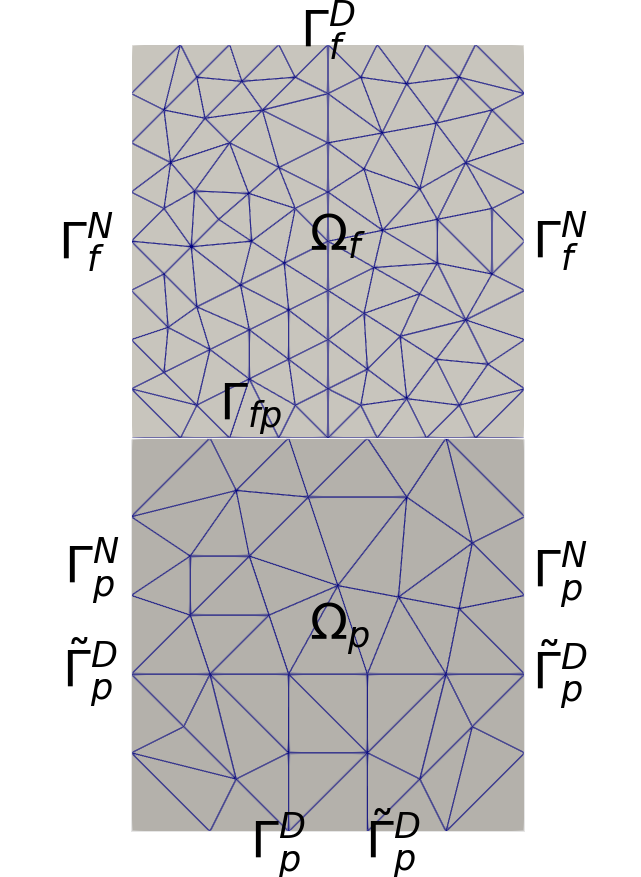
$$\mu=1,\quad\alpha_{p}=1,\quad\lambda_{p}=1,\quad\mu_{p}=1,\quad s_{0}=1,\quad\mathbf{K}=\mathbf{I},\quad\alpha_{\mathtt{BJS}}=1,$$

$$\mathbf{u}_{f}=\pi\,\cos(\pi\,t)\left(\begin{array}[]{c}-3x+\cos(y)\\ y+1\end{array}\right),$$

$$p_{f}=\exp(t)\,\sin(\pi\,x)\,\cos\left(\frac{\pi\,y}{2}\right)+2\,\pi\,\cos(\pi\,t),$$

$$p_{p}=\exp(t)\,\sin(\pi\,x)\,\cos\left(\frac{\pi\,y}{2}\right),$$

$$\mathbf{u}_{p}=-\frac{1}{\mu}\,\mathbf{K}\,\nabla p_{p},\quad{\boldsymbol{\eta}}_{p}=\sin(\pi\,t)\,\left(\begin{array}[]{c}-3x+\cos(y)\\ y+1\end{array}\right).$$

Figure 7.1: Example 1, domain and coarsest mesh level (left), parameters and analytical solution (right).

Tables 7.1 and 7.2 show the convergence history for a sequence of quasi-uniform mesh refinements with non-matching grids along the interface employing conforming and non-conforming spaces for the Lagrange multipliers (cf. (5.1)–(5.2)), respectively. In the tables, $h_{f}$ and $h_{p}$ denote the mesh sizes in $\Omega_{f}$ and $\Omega_{p}$, respectively, while the mesh sizes for their traces on $\Gamma_{fp}$ are $h_{tf}$ and $h_{tp}$, satisfying $h_{tf}=\frac{5}{8}\,h_{tp}$. We note that the Stokes pressure and the displacement at time $t_{m}$ are recovered by the post-processed formulae $p^{m}_{f}=-\frac{1}{n}(\mathrm{tr}({\boldsymbol{\sigma}}^{m}_{f})-2\,\mu\,q^{m}_{f})$ (cf. (2.2)) and ${\boldsymbol{\eta}}^{m}_{p}={\boldsymbol{\eta}}^{m-1}_{p}+\Delta t\,\mathbf{u}^{m}_{s}$ (cf. Remark 5.3), respectively. The results illustrate that spatial rates of convergence $\mathcal{O}(h)$, as provided by Theorem 6.5, are attained for all subdomain variables in their natural norms. The Lagrange multiplier variables, which are approximated in $\mathbf{P}_{1}-\mathbf{P}_{1}-\mathrm{P}_{1}$ and $\mathbf{P}^{\mathrm{dc}}_{1}-\mathbf{P}^{\mathrm{dc}}_{1}-\mathrm{P}^{\mathrm{dc}}_{1}$, exhibit rates of convergence $\mathcal{O}(h^{3/2})$ and $\mathcal{O}(h^{2})$ in the $\mathrm{H}^{1/2}$ and $\mathrm{L}^{2}$-norms on $\Gamma_{fp}$, respectively, which is consistent with the order of approximation.

	$\|{\mathbf{e}}_{{\boldsymbol{\sigma}}_{f}}\|_{\ell^{2}(0,T;\mathbb{X}_{f})}$		$\|{\mathbf{e}}_{\mathbf{u}_{f}}\|_{\ell^{2}(0,T;\mathbf{V}_{f})}$		$\|{\mathbf{e}}_{{\boldsymbol{\gamma}}_{f}}\|_{\ell^{2}(0,T;\mathbb{Q}_{f})}$		$\|{\mathbf{e}}_{p_{f}}\|_{\ell^{2}(0,T;\mathrm{L}^{2}(\Omega_{f}))}$
$h_{f}$	error	rate	error	rate	error	rate	error	rate
0.1964	2.2E-02	–	2.7E-02	–	2.4E-03	–	6.3E-03	–
0.0997	1.2E-02	0.95	1.4E-02	1.00	9.3E-04	1.41	3.1E-03	1.05
0.0487	5.7E-03	0.99	6.8E-03	0.99	4.2E-04	1.11	1.6E-03	0.93
0.0250	2.9E-03	1.04	3.4E-03	1.04	2.0E-04	1.13	7.8E-04	1.07
0.0136	1.4E-03	1.14	1.7E-03	1.15	9.4E-05	1.23	3.9E-04	1.15
0.0072	7.1E-04	1.08	8.4E-04	1.10	4.7E-05	1.09	2.0E-04	1.02

	$\|{\mathbf{e}}_{{\boldsymbol{\sigma}}_{p}}\|_{\ell^{\infty}(0,T;\mathbb{X}_{p})}$		$\|{\mathbf{e}}_{\mathbf{u}_{s}}\|_{\ell^{2}(0,T;\mathbf{V}_{s})}$		$\|{\mathbf{e}}_{{\boldsymbol{\gamma}}_{p}}\|_{\ell^{2}(0,T;\mathbb{Q}_{p})}$		$\|{\mathbf{e}}_{\mathbf{u}_{p}}\|_{\ell^{2}(0,T;\mathbf{V}_{p})}$		$\|{\mathbf{e}}_{p_{p}}\|_{\ell^{\infty}(0,T;\mathrm{W}_{p})}$
$h_{p}$	error	rate	error	rate	error	rate	error	rate	error	rate
0.2828	2.7E-01	–	4.3E-02	–	3.4E-02	–	1.0E-01	–	7.5E-02	–
0.1646	1.4E-01	1.27	2.2E-02	1.23	9.4E-03	2.38	5.2E-02	1.27	3.8E-02	1.25
0.0779	6.7E-02	0.97	1.1E-02	0.96	2.2E-03	1.96	2.5E-02	1.00	1.9E-02	0.93
0.0434	3.4E-02	1.17	5.4E-03	1.19	5.8E-04	2.25	1.2E-02	1.24	9.4E-03	1.22
0.0227	1.7E-02	1.06	2.7E-03	1.07	2.0E-04	1.68	5.9E-03	1.08	4.7E-03	1.07
0.0124	8.4E-03	1.15	1.4E-03	1.15	8.1E-05	1.48	2.9E-03	1.15	2.4E-03	1.14

$\|{\mathbf{e}}_{{\boldsymbol{\eta}}_{p}}\|_{\ell^{2}(0,T;\mathbf{L}^{2}(\Omega_{p}))}$			$\|{\mathbf{e}}_{{\boldsymbol{\varphi}}}\|_{\ell^{2}(0,T;{\boldsymbol{\Lambda}}_{f})}$			$\|{\mathbf{e}}_{{\boldsymbol{\theta}}}\|_{\ell^{2}(0,T;{\boldsymbol{\Lambda}}_{s}))}$		$\|{\mathbf{e}}_{\lambda}\|_{\ell^{2}(0,T;\Lambda_{p})}$
error	rate	$h_{tf}$	error	rate	$h_{tp}$	error	rate	error	rate
2.7E-04	–	1/8	1.6E-03	–	1/5	1.6E-02	–	6.9E-03	–
1.4E-04	1.23	1/16	3.7E-04	2.11	1/10	5.7E-03	1.49	2.5E-03	1.49
6.7E-05	0.96	1/32	1.3E-04	1.45	1/20	1.2E-03	2.31	8.5E-04	1.52
3.4E-05	1.19	1/64	4.6E-05	1.54	1/40	3.4E-04	1.76	3.0E-04	1.50
1.7E-05	1.07	1/128	1.2E-05	1.96	1/80	1.1E-04	1.62	1.1E-04	1.50
8.4E-06	1.15	1/256	3.6E-06	1.70	1/160	2.2E-05	2.34	3.7E-05	1.54

Table 7.1: Example 1, errors and convergence rates with $\mathbf{P}_{1}-\mathbf{P}_{1}-\mathrm{P}_{1}$ Lagrange multipliers.

	$\|{\mathbf{e}}_{{\boldsymbol{\sigma}}_{f}}\|_{\ell^{2}(0,T;\mathbb{X}_{f})}$		$\|{\mathbf{e}}_{\mathbf{u}_{f}}\|_{\ell^{2}(0,T;\mathbf{V}_{f})}$		$\|{\mathbf{e}}_{{\boldsymbol{\gamma}}_{f}}\|_{\ell^{2}(0,T;\mathbb{Q}_{f})}$		$\|{\mathbf{e}}_{p_{f}}\|_{\ell^{2}(0,T;\mathrm{L}^{2}(\Omega_{f}))}$
$h_{f}$	error	rate	error	rate	error	rate	error	rate
0.1964	2.2E-02	–	2.7E-02	–	2.4E-03	–	6.1E-03	–
0.0997	1.2E-02	0.94	1.4E-02	1.00	9.7E-04	1.31	3.1E-03	1.02
0.0487	5.7E-03	0.99	6.8E-03	0.99	4.2E-04	1.16	1.6E-03	0.92
0.0250	2.8E-03	1.04	3.4E-03	1.04	2.0E-04	1.13	7.8E-04	1.07
0.0136	1.4E-03	1.14	1.7E-03	1.15	9.4E-05	1.23	3.9E-04	1.15
0.0072	7.1E-04	1.08	8.4E-04	1.09	4.7E-05	1.09	2.0E-04	1.02

	$\|{\mathbf{e}}_{{\boldsymbol{\sigma}}_{p}}\|_{\ell^{\infty}(0,T;\mathbb{X}_{p})}$		$\|{\mathbf{e}}_{\mathbf{u}_{s}}\|_{\ell^{2}(0,T;\mathbf{V}_{s})}$		$\|{\mathbf{e}}_{{\boldsymbol{\gamma}}_{p}}\|_{\ell^{2}(0,T;\mathbb{Q}_{p})}$		$\|{\mathbf{e}}_{\mathbf{u}_{p}}\|_{\ell^{2}(0,T;\mathbf{V}_{p})}$		$\|{\mathbf{e}}_{p_{p}}\|_{\ell^{\infty}(0,T;\mathrm{W}_{p})}$
$h_{p}$	error	rate	error	rate	error	rate	error	rate	error	rate
0.2828	2.7E-01	–	4.3E-02	–	3.4E-02	–	1.0E-01	–	7.5E-02	–
0.1646	1.4E-01	1.27	2.2E-02	1.23	9.4E-03	2.39	5.2E-02	1.26	3.8E-02	1.25
0.0779	6.7E-02	0.97	1.1E-02	0.96	2.2E-03	1.96	2.5E-02	1.00	1.9E-02	0.93
0.0434	3.4E-02	1.17	5.4E-03	1.19	5.8E-04	2.25	1.2E-02	1.24	9.4E-03	1.22
0.0227	1.7E-02	1.06	2.7E-03	1.07	2.0E-04	1.67	5.9E-03	1.08	4.7E-03	1.07
0.0124	8.4E-03	1.15	1.4E-03	1.15	8.1E-05	1.48	2.9E-03	1.15	2.4E-03	1.14

$\|{\mathbf{e}}_{{\boldsymbol{\eta}}_{p}}\|_{\ell^{2}(0,T;\mathbf{L}^{2}(\Omega_{p}))}$			$\|{\mathbf{e}}_{{\boldsymbol{\varphi}}}\|_{\ell^{2}(0,T;\mathbf{L}^{2}(\Gamma_{fp}))}$			$\|{\mathbf{e}}_{{\boldsymbol{\theta}}}\|_{\ell^{2}(0,T;\mathbf{L}^{2}(\Gamma_{fp}))}$		$\|{\mathbf{e}}_{\lambda}\|_{\ell^{2}(0,T;\mathrm{L}^{2}(\Gamma_{fp}))}$
error	rate	$h_{tf}$	error	rate	$h_{tp}$	error	rate	error	rate
2.7E-04	–	1/8	4.1E-04	–	1/5	7.9E-03	–	1.1E-03	–
1.4E-04	1.23	1/16	2.0E-04	1.04	1/10	2.9E-03	1.46	3.1E-04	1.87
6.7E-05	0.96	1/32	2.4E-05	3.07	1/20	5.7E-04	2.34	7.7E-05	2.01
3.4E-05	1.19	1/64	6.4E-06	1.89	1/40	1.5E-04	1.89	1.9E-05	2.00
1.7E-05	1.07	1/128	1.6E-06	1.97	1/80	3.8E-05	2.01	4.9E-06	1.98
8.4E-06	1.15	1/256	4.0E-07	2.02	1/160	9.0E-06	2.09	1.2E-06	2.09

Table 7.2: Example 1, errors and convergence rates with $\mathbf{P}^{\mathrm{dc}}_{1}-\mathbf{P}^{\mathrm{dc}}_{1}-\mathrm{P}^{\mathrm{dc}}_{1}$ Lagrange multipliers.

7.2 Example 2: coupled surface and subsurface flows

In this example, we simulate coupling of surface and subsurface flows, which could be used to describe the interaction between a river and an aquifer. We consider the domain $\Omega=(0,2)\times(-1,1)$. We associate the upper half with the river flow modeled by Stokes equations, while the lower half represents the flow in the aquifer governed by the Biot system. The appropriate interface conditions are enforced along the interface $y=0$. In this example we focus on the qualitative behavior of the solution and use unit physical parameters:

$$\mu=1,\quad\alpha_{p}=1,\quad\lambda_{p}=1,\quad\mu_{p}=1,\quad s_{0}=1,\quad\mathbf{K}=\mathbf{I},\quad\alpha_{\mathtt{BJS}}=1.$$

The body forces terms and external source are set to zero, as well as the initial conditions. The flow is driven through a parabolic fluid velocity on the left boundary of the fluid region with boundary conditions specified as follows:

$$\begin{array}[]{lll}\displaystyle\mathbf{u}_{f}=(-40y(y-1)\ \ 0)^{t}&\mbox{on}&\Gamma_{f,left},\\[4.30554pt] \displaystyle\mathbf{u}_{f}={\mathbf{0}}&\mbox{on}&\Gamma_{f,top},\\[4.30554pt] \displaystyle{\boldsymbol{\sigma}}_{f}{\mathbf{n}}_{f}={\mathbf{0}}&\mbox{on}&\Gamma_{f,right},\\[4.30554pt] \displaystyle p_{p}=0{\quad\hbox{and}\quad}{\boldsymbol{\sigma}}_{p}{\mathbf{n}}_{p}={\mathbf{0}}&\mbox{on}&\Gamma_{p,bottom},\\[4.30554pt] \displaystyle\mathbf{u}_{p}\cdot{\mathbf{n}}_{p}=0{\quad\hbox{and}\quad}\mathbf{u}_{s}={\mathbf{0}}&\mbox{on}&\Gamma_{p,left}\cup\Gamma_{p,right}.\end{array}$$

The simulation is run for a total time $T=3$ with a time step $\Delta t=0.06$. The computed solution is presented in Figure 7.2.

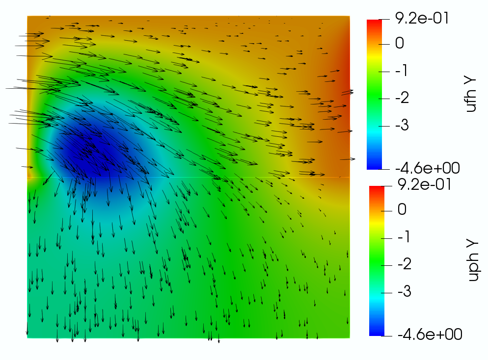
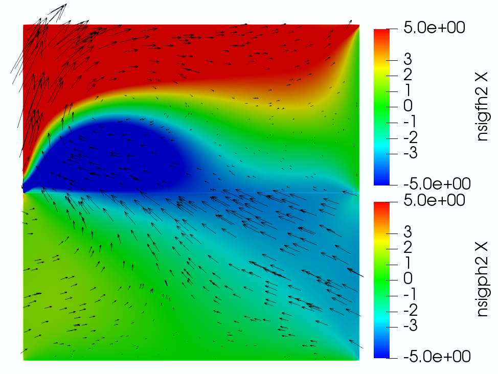
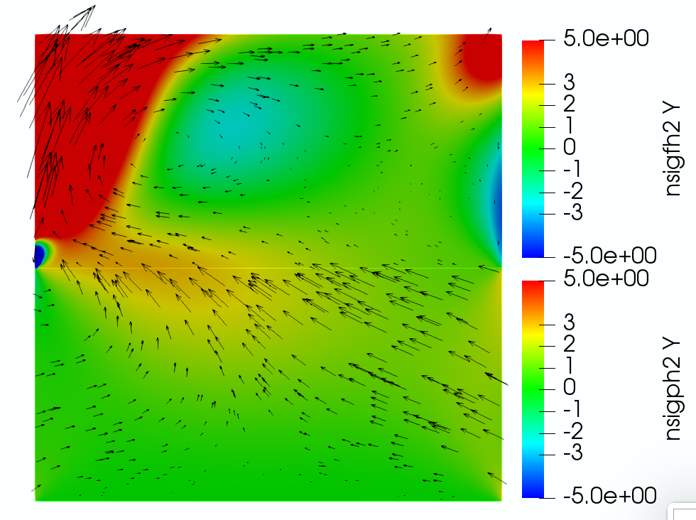
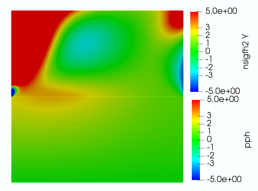
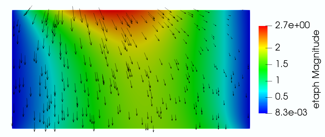
Figure 7.2: Example 2, computed solution at $T=3$. Top left: velocities $\mathbf{u}_{fh}$ and $\mathbf{u}_{ph}$ (arrows), $\mathbf{u}_{fh,2}$ and $\mathbf{u}_{ph,2}$ (color). Top middle and right: negative stresses $-({\boldsymbol{\sigma}}_{fh,12},{\boldsymbol{\sigma}}_{fh,22})^{\mathrm{t}}$ and $-({\boldsymbol{\sigma}}_{ph,12},{\boldsymbol{\sigma}}_{ph,22})^{\mathrm{t}}$ (arrows); middle: $-{\boldsymbol{\sigma}}_{fh,12}$ and $-{\boldsymbol{\sigma}}_{ph,12}$ (color); right: $-{\boldsymbol{\sigma}}_{fh,22}$ and $-{\boldsymbol{\sigma}}_{ph,22}$ (color). Bottom left: negative Stokes stress $-{\boldsymbol{\sigma}}_{fh,22}$ and Darcy pressure $p_{ph}$. Bottom right: displacement ${\boldsymbol{\eta}}_{ph}$ (arrows) and its magnitude (color).

From the velocity plot (top left), we see that the flow in the Stokes region is moving primarily from left to right, driven by the parabolic inflow condition, with some of the fluid percolating downward into the poroelastic medium due to the zero pressure at the bottom, which simulates gravity. The mass conservation $\mathbf{u}_{f}\cdot{\mathbf{n}}_{f}+\left(\partial_{t}{\boldsymbol{\eta}}_{p}+\mathbf{u}_{p}\right)\cdot{\mathbf{n}}_{p}=0$ on the interface with ${\mathbf{n}}_{p}=(0,1)^{\mathrm{t}}$ indicates the continuity of the second components of the fluid velocity and Darcy velocity when the displacement becomes steady, which is observed from the color plot of the vertical velocity. The stress plots (top middle and right) illustrate the ability of our fully mixed formulation to compute accurate $\mathbb{H}(\mathbf{div})$ stresses in both the fluid and poroelastic regions, without the need for numerical differentiation. In addition, the conservation of momentum ${\boldsymbol{\sigma}}_{f}{\mathbf{n}}_{f}+{\boldsymbol{\sigma}}_{p}{\mathbf{n}}_{p}={\mathbf{0}}$ and balance of normal stress $({\boldsymbol{\sigma}}_{f}{\mathbf{n}}_{f})\cdot{\mathbf{n}}_{f}=-p_{p}$ imply that ${\boldsymbol{\sigma}}_{f,12}={\boldsymbol{\sigma}}_{p,12}$, ${\boldsymbol{\sigma}}_{f,22}={\boldsymbol{\sigma}}_{p,22}$ and $-{\boldsymbol{\sigma}}_{f,22}=p_{p}$ on the interface. These conditions are verified from the top middle and right color plots, as well as the bottom left plot. Furthermore, the arrows in the stress plots are formed by the second columns of the stresses, whose traces on the interface are ${\boldsymbol{\sigma}}_{f}{\mathbf{n}}_{f}$ and $-{\boldsymbol{\sigma}}_{p}{\mathbf{n}}_{p}$, respectively. For visualization purpose, the Stokes stress is scaled by a factor of $1/5$ compared to the poroelastic stress, due to large difference in their magnitudes away from the interface. Nevertheless, the continuity of the vector field across the interface is evident, consistent with the conservation of momentum condition ${\boldsymbol{\sigma}}_{f}{\mathbf{n}}_{f}+{\boldsymbol{\sigma}}_{p}{\mathbf{n}}_{p}={\mathbf{0}}$. The overall qualitative behavior of the computed stresses is consistent with the specified boundary and interface conditions. In particular, we observe large fluid stress along the top boundary due to the no slip condition, as well as along the interface due to the slip with friction condition. The singularity near the lower left corner of the Stokes region is due to the mismatch in boundary conditions between the fluid and poroelastic regions. Finally, the last plot shows that the inflow from the Stokes region causes deformation of the poroelastic medium.

7.3 Example 3: irregularly shaped fluid-filled cavity

This example features highly irregularly shaped cavity motivated by modeling flow through vuggy or naturally fractured reservoirs or aquifers. It uses physical units and realistic parameter values taken from the reservoir engineering literature [37]:

$$\begin{array}[]{c}\mu=10^{-6}\text{ kPa s},\quad\alpha_{p}=1,\quad\lambda_{p}=5/18\times 10^{7}\text{ kPa},\quad\mu_{p}=5/12\times 10^{7}\text{ kPa},\\[8.61108pt] s_{0}=6.89\times 10^{-2}\text{ kPa}^{-1},\quad\mathbf{K}=10^{-8}\times\mathbf{I}\text{ m}^{2},\quad\alpha_{\mathtt{BJS}}=1.\end{array}$$

We emphasize that the problem features very small permeability and storativity, as well as large Lamé parameters. These are parameter regimes that are known to lead locking in modeling of the Biot system of poroelasticity [45, 60]. The domain is $\Omega=(0,1)\times(0,1)$, with a large fluid-filled cavity in the interior. The body forces and external sources are set to zero. The flow is driven from left to right via a pressure drop of 1 kPa, with boundary conditions specified as follows:

$$\begin{array}[]{l}{\boldsymbol{\sigma}}_{f}{\mathbf{n}}_{f}\cdot{\mathbf{n}}_{f}=1000,\quad\mathbf{u}_{f}\cdot{\mathbf{t}}_{f}=0{\quad\hbox{on}\quad}\Gamma_{f,right},\\[8.61108pt] p_{p}=1001{\quad\hbox{on}\quad}\Gamma_{p,left},\quad p_{p}=1000{\quad\hbox{on}\quad}\Gamma_{p,right}{\quad\hbox{and}\quad}\mathbf{u}_{p}\cdot{\mathbf{n}}_{p}=0{\quad\hbox{on}\quad}\Gamma_{p,top}\cup\Gamma_{p,bottom},\\[8.61108pt] {\boldsymbol{\sigma}}_{p}\,{\mathbf{n}}_{p}=-\alpha_{p}\,p_{p}\,{\mathbf{n}}_{p}{\quad\hbox{on}\quad}\Gamma_{p,left}\cup\Gamma_{p,right}{\quad\hbox{and}\quad}\mathbf{u}_{s}={\mathbf{0}}{\quad\hbox{on}\quad}\Gamma_{p,top}\cup\Gamma_{p,bottom}.\end{array}$$

The total simulation time is $T=10\,$s with a time step of size $\Delta t=0.05\,$s. To avoid inconsistency between the initial and boundary conditions for $p_{p}$, we start with $p_{p}=1000$ on $\Gamma_{p,left}$ and gradually increase it to reach $p_{p}=1001$ at $t=0.5\,$s. Similar adjustment is done for ${\boldsymbol{\sigma}}_{p}{\mathbf{n}}_{p}$.

The simulation results at the final time $T=10\,$s are shown in Figure 7.3. In the top plots, we present the Darcy pressure and Darcy velocity vector, the displacement vector with its magnitude, and the first row of the poroelastic stress with its magnitude. Since the pressure variation is small relative to its value, for visualization purpose we plot its difference from the reference pressure, $p_{p}-1000$. The Darcy velocity and the pressure drop are largest in the region between the left inflow boundary and the cavity. The displacement is largest around the cavity, due to the large fluid velocity within the cavity and the slip with friction interface condition. The poroelastic stress exhibits singularities near some of the sharp tips of the cavity. The bottom plots show the fluid pressure and velocity vector, the velocity vector with its magnitude, and the first row of the fluid stress with its magnitude. Similarly to the Darcy pressure, we plot $p_{f}-1000$. A channel-like flow profile is clearly visible within the cavity, with the largest velocity along a central path away from the cavity walls. The fluid pressure is decreasing from left to right along the central path of the cavity. Consistent with the poroelastic stress, the fluid stress near the tips of the cavity is relatively larger. We emphasize that, despite the locking regime of the parameters, the computed solution is free of locking and spurious oscillations. This example illustrates the ability of our method to handle computationally challenging problems with physically realistic parameters in poroelastic locking regimes.

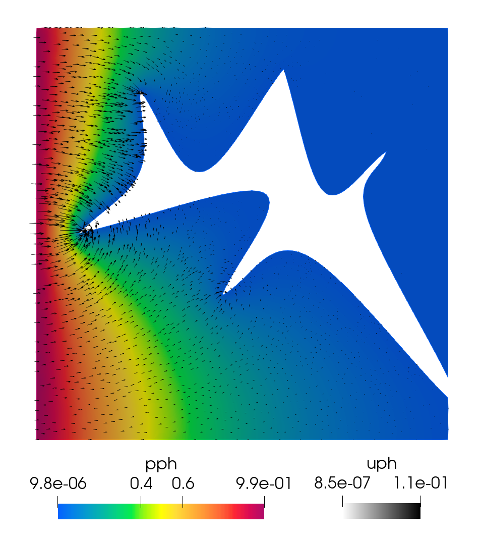
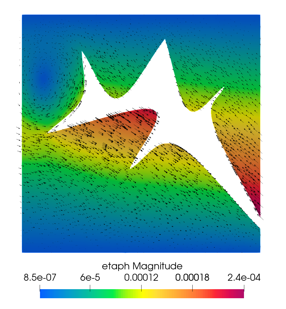
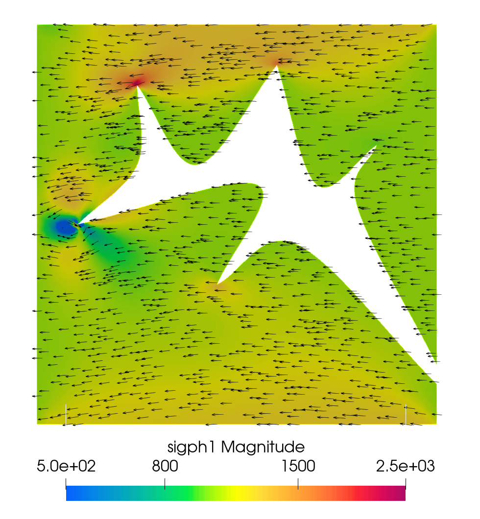
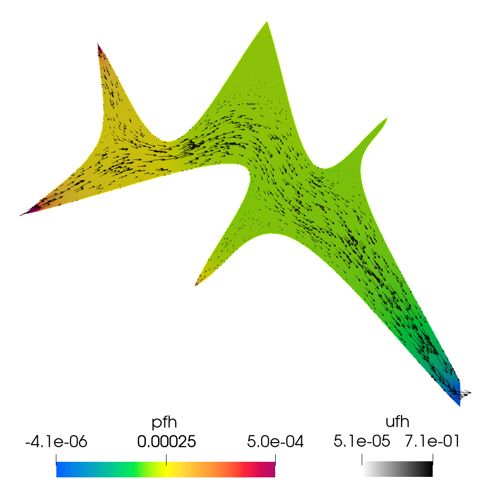
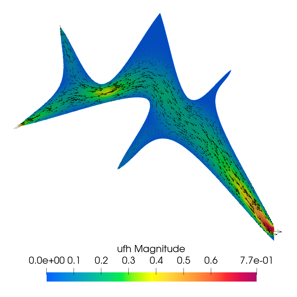
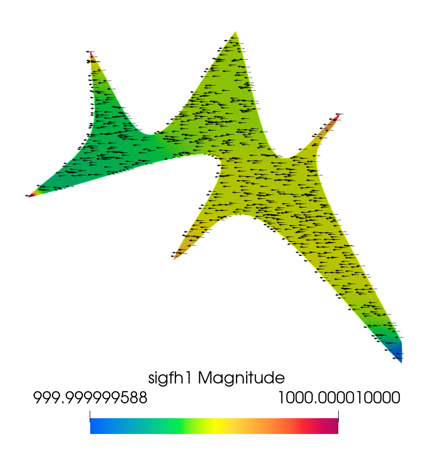
Figure 7.3: Example 3, computed solution at $T=10\,$s. Top left: Darcy velocity (arrows) and pressure (color). Top middle: displacement (arrows) and its magnitude (color). Top right: first row of the poroelastic stress tensor (arrows) and its magnitude (color). Bottom left: Stokes velocity (arrows) and pressure (color). Bottom middle: Stokes velocity (arrows) and its magnitude (color). Bottom right: first row of the Stokes stress (arrows) and its magnitude (color).

8 Conclusions

In this paper we present and analyze the first, to the best of our knowledge, fully dual mixed formulation of the quasi-static Stokes-Biot model, and its mixed finite element approximation, using a velocity-pressure Darcy formulation, a weakly symmetric stress-displacement-rotation elasticity formulation, and a weakly symmetric stress-velocity-vorticity Stokes formulation. Essential-type interface conditions are imposed via suitable Lagrange multipliers. The numerical method features accurate stresses and Darcy velocity with local mass and momentum conservation. Furthermore, a new multipoint stress-flux mixed finite element method is developed that allows for local elimination of the Darcy velocity, the fluid and poroelastic stresses, the vorticity, and the rotation, resulting in a reduced positive definite cell-centered pressure-velocities-traces system. The theoretical results are complemented by a series of numerical experiments that illustrate the convergence rates for all variables in their natural norms, as well as the ability of the method to simulate physically realistic problems motivated by applications to coupled surface-subsurface flows and flows in fractured poroelastic media with parameter values in locking regimes.

References

• [1] J. A. Almonacid, H. S. Díaz, G. N. Gatica, and A. Márquez. A fully-mixed finite element method for the Darcy–Forchheimer/Stokes coupled problem. IMA J. Numer. Anal., 40(2):1454–1502, 2020.
• [2] M. Amara and J. M. Thomas. Equilibrium finite elements for the linear elastic problem. Numer. Math., 33(4):367–383, 1979.
• [3] I. Ambartsumyan, V. J. Ervin, T. Nguyen, and I. Yotov. A nonlinear Stokes-Biot model for the interaction of a non-Newtonian fluid with poroelastic media. ESAIM Math. Model. Numer. Anal., 53(6):1915–1955, 2019.
• [4] I. Ambartsumyan, E. Khattatov, T. Nguyen, and I. Yotov. Flow and transport in fractured poroelastic media. GEM Int. J. Geomath., 10(1):1–34, 2019.
• [5] I. Ambartsumyan, E. Khattatov, J. M. Nordbotten, and I. Yotov. A multipoint stress mixed finite element method for elasticity on simplicial grids. SIAM J. Numer. Anal., 58(1):630–656, 2020.
• [6] I. Ambartsumyan, E. Khattatov, J. M. Nordbotten, and I. Yotov. A multipoint stress mixed finite element method for elasticity on quadrilateral grids. Numer. Methods Partial Differential Equations, 37(3):1886–1915, 2021.
• [7] I. Ambartsumyan, E. Khattatov, and I. Yotov. A coupled multipoint stress–multipoint flux mixed finite element method for the Biot system of poroelasticity. Comput. Methods Appl. Mech. Engrg., 372:113407, 2020.
• [8] I. Ambartsumyan, E. Khattatov, I. Yotov, and P. Zunino. A Lagrange multiplier method for a Stokes-Biot fluid-poroelastic structure interaction model. Numer. Math., 140(2):513–553, 2018.
• [9] D. N. Arnold, F. Brezzi, and J. Douglas. PEERS: a new mixed finite element for plane elasticity. Japan J. Appl. Math., 1(2):347–367, 1984.
• [10] D. N. Arnold, R. S. Falk, and R. Winter. Mixed finite element methods for linear elasticity with weakly imposed symmetry. Math. Comp., 76(260):1699–1723, 2007.
• [11] G. Awanou. Rectangular mixed elements for elasticity with weakly imposed symmetry condition. Adv. Comput. Math., 38(2):351–367, 2013.
• [12] S. Badia, A. Quaini, and A. Quarteroni. Coupling Biot and Navier-Stokes equations for modelling fluid-poroelastic media interaction. J. Comput. Phys., 228(21):7986–8014, 2009.
• [13] E. A. Bergkamp, C. V. Verhoosel, J. J. C. Remmers, and D. M. J. Smeulders. A staggered finite element procedure for the coupled Stokes-Biot system with fluid entry resistance. Comput. Geosci., 24(4):1497–1522, 2020.
• [14] M. Biot. General theory of three-dimensional consolidation. J. Appl. Phys., 12:155–164, 1941.
• [15] D. Boffi, F. Brezzi, L. F. Demkowicz, R. G. Durán, R. S. Falk, and M. Fortin. Mixed finite elements, compatibility conditions, and applications, volume 1939 of Lecture Notes in Mathematics. Springer-Verlag, Berlin; Fondazione C.I.M.E., Florence, 2008.
• [16] D. Boffi, F. Brezzi, and M. Fortin. Reduced symmetry elements in linear elasticity. Commun. Pure Appl. Anal., 8(1):95–121, 2009.
• [17] F. Brezzi, J. Douglas, and L. D. Marini. Two families of mixed finite elements for second order elliptic problems. Numer. Math., 47(2):217–235, 1985.
• [18] F. Brezzi and M. Fortin. Mixed and Hybrid Finite Element Methods. Springer Series in Computational Mathematics, 15. Springer-Verlag, New York, 1991.
• [19] F. Brezzi, M. Fortin, and L. D. Marini. Error analysis of piecewise constant pressure approximations of Darcy’s law. Comput. Methods Appl. Mech. Eng., 195:1547–1559, 2006.
• [20] M. Bukac, I. Yotov, R. Zakerzadeh, and P. Zunino. Partitioning strategies for the interaction of a fluid with a poroelastic material based on a Nitsche’s coupling approach. Comput. Methods Appl. Mech. Engrg., 292:138–170, 2015.
• [21] M. Bukac, I. Yotov, and P. Zunino. An operator splitting approach for the interaction between a fluid and a multilayered poroelastic structure. Numer. Methods Partial Differential Equations, 31(4):1054–1100, 2015.
• [22] M. Bukac, I. Yotov, and P. Zunino. Dimensional model reduction for flow through fractures in poroelastic media. ESAIM Math. Model. Numer. Anal., 51(4):1429–1471, 2017.
• [23] A. Cesmelioglu and P. Chidyagwai. Numerical analysis of the coupling of free fluid with a poroelastic material. Numer. Methods Partial Differential Equations, 36(3):463–494, 2020.
• [24] A. Cesmelioglu, H. Lee, A. Quaini, K. Wang, and S.-Y. Yi. Optimization-based decoupling algorithms for a fluid-poroelastic system. In Topics in numerical partial differential equations and scientific computing, volume 160 of IMA Vol. Math. Appl., pages 79–98. Springer, New York, 2016.
• [25] S. Cesmelioglu. Analysis of the coupled Navier-Stokes/Biot problem. J. Math. Anal. Appl., 456(2):970–991, 2017.
• [26] P. Ciarlet. The Finite Element Method for Elliptic Problems. Studies in Mathematics and its Applications, Vol. 4. North-Holland Publishing Co., Amsterdam-New York-Oxford, 1978.
• [27] B. Cockburn, J. Gopalakrishnan, and J. Guzmán. A new elasticity element made for enforcing weak stress symmetry. Math. Comp., 79(271):1331–1349, 2010.
• [28] T. Davis. Algorithm 832: UMFPACK V4.3 - an unsymmetric-pattern multifrontal method. ACM Trans. Math. Software, 30(2):196–199, 2004.
• [29] V. J. Ervin, E. W. Jenkins, and S. Sun. Coupled generalized nonlinear Stokes flow with flow through a porous medium. SIAM J. Numer. Anal., 47(2):929–952, 2009.
• [30] M. Farhloul and M. Fortin. Dual hybrid methods for the elasticity and the Stokes problems: a unified approach. Numer. Math., 76(4):419–440, 1997.
• [31] J. Galvis and M. Sarkis. Non-matching mortar discretization analysis for the coupling Stokes-Darcy equations. Electron. Trans. Numer. Anal., 26:350–384, 2007.
• [32] G. N. Gatica. A Simple Introduction to the Mixed Finite Element Method. Theory and Applications. Springer Briefs in Mathematics. Springer, Cham, 2014.
• [33] G. N. Gatica, N. Heuer, and S. Meddahi. On the numerical analysis of nonlinear twofold saddle point problems. IMA J. Numer. Anal., 23(2):301–330, 2003.
• [34] G. N. Gatica, A. Márquez, R. Oyarzúa, and R. Rebolledo. Analysis of an augmented fully-mixed approach for the coupling of quasi-Newtonian fluids and porous media. Comput. Methods Appl. Mech. Engrg., 270:76–112, 2014.
• [35] G. N. Gatica, R. Oyarzúa, and F. J. Sayas. Analysis of fully-mixed finite element methods for the Stokes–Darcy coupled problem. Math. Comp., 80(276):1911–1948, 2011.
• [36] G. N. Gatica, R. Oyarzúa, and F. J. Sayas. A twofold saddle point approach for the coupling of fluid flow with nonlinear porous media flow. IMA J. Numer. Anal., 32(3):845–887, 2012.
• [37] V. Girault, M. F. Wheeler, B. Ganis, and M. E. Mear. A lubrication fracture model in a poroelastic medium. Math. Models Methods Appl. Sci., 25(4):587–645, 2015.
• [38] F. Hecht. New development in FreeFem++. J. Numer. Math., 20(3-4):251–265, 2012.
• [39] R. Horn and C. R. Johnson. Matrix analysis. Corrected reprint of the 1985 original. Cambridge University Press, Cambridge, 1990.
• [40] R. Ingram, M. F. Wheeler, and I. Yotov. A multipoint flux mixed finite element method on hexahedra. SIAM J. Math. Anal., 48(4):1281–1312, 2010.
• [41] E. Keilegavlen and J. M. Nordbotten. Finite volume methods for elasticity with weak symmetry. Int. J. Numer. Meth. Engng., 112(8):939–962, 2017.
• [42] E. Khattatov and I. Yotov. Domain decomposition and multiscale mortar mixed finite element methods for linear elasticity with weak stress symmetry. ESAIM Math. Model. Numer. Anal., 53(6):2081–2108, 2019.
• [43] R. A. Klausen and R. Winther. Robust convergence of multi point flux approximation on rough grids. Numer. Math., 104(3):317–337, 2006.
• [44] H. Kunwar, H. Lee, and K. Seelman. Second-order time discretization for a coupled quasi-Newtonian fluid-poroelastic system. Internat. J. Numer. Methods Fluids, 92(7):687–702, 2020.
• [45] J. J. Lee. Robust error analysis of coupled mixed methods for Biot’s consolidation model. J. Sci. Comput., 69(2):610–632, 2016.
• [46] J. J. Lee. Towards a unified analysis of mixed methods for elasticity with weakly symmetric stress. Adv. Comput. Math., 42(2):361–376, 2016.
• [47] T. Li and I. Yotov. A mixed elasticity formulation for fluid–poroelastic structure interaction. arXiv:2011.00132v2 [math.NA].
• [48] J.-C. Nédélec. A new family of mixed finite elements in ${\bf R}^{3}$. Numer. Math., 50(1):57–81, 1986.
• [49] J. M. Nordbotten. Cell-centered finite volume discretizations for deformable porous media. Internat. J. Numer. Methods Engrg., 100(6):399–418, 2014.
• [50] J. M. Nordbotten. Convergence of a cell-centered finite volume discretization for linear elasticity. SIAM J. Numer. Anal., 53(6):2605–2625, 2015.
• [51] J. M. Nordbotten. Stable cell-centered finite volume discretization for Biot equations. SIAM J. Numer. Anal., 54(2):942–968, 2016.
• [52] R. E. Showalter. Monotone Operators in Banach Space and Nonlinear Partial Differential Equations. Mathematical Surveys and Monographs, 49. American Mathematical Society, Providence, RI, 1997.
• [53] R. E. Showalter. Poroelastic filtration coupled to Stokes flow. Control theory of partial differential equations. Lect. Notes Pure Appl. Math., 242, Chapman & Hall/CRC, Boca Raton, FL, pages 229–241, 2005.
• [54] R. E. Showalter. Nonlinear degenerate evolution equations in mixed formulations. SIAM J. Math. Anal., 42(5):2114–2131, 2010.
• [55] R. Stenberg. A family of mixed finite elements for the elasticity problem. Numer. Math., 53(5):513–538, 1988.
• [56] J. Wen and Y. He. A strongly conservative finite element method for the coupled Stokes-Biot model. Comput. Math. Appl., 80(5):1421–1442, 2020.
• [57] M. F. Wheeler, G. Xue, and I. Yotov. A multipoint flux mixed finite element method on distorted quadrilaterals and hexahedra. Numer. Math., 121(1):165–204, 2012.
• [58] M. F. Wheeler and I. Yotov. A multipoint flux mixed finite element method. SIAM J. Numer. Anal., 44(5):2082–2106, 2006.
• [59] S.-Y. Yi. Convergence analysis of a new mixed finite element method for Biot’s consolidation model. Numer. Methods Partial Differential Equations, 30(4):1189–1210, 2014.
• [60] S.-Y. Yi. A study of two modes of locking in poroelasticity. SIAM J. Numer. Anal., 55(4):1915–1936, 2017.