A population of compact radio variables and transients in the radio bright zone at the Galactic center observed with the Jansky Very Large Array

Abstract

Using JVLA data obtained from high-resolution observations at 5.5 GHz at multiple epochs in 2014 and 2019, we have detected a population of radio variables and transients in the radio bright zone at the Galactic center. With observations covering a sky area of 180 arcmin² at an angular resolution of 0.4 arcsec, we report new detections of 110 Galactic center compact radio (GCCR) sources with a size of $<1$ arcsec. The flux densities of GCCRs exceed 70 $\mu$Jy, with at least 10$\sigma$ significance. Among these sources, 82 are variable or transient and 28 are non-variable. About 10% of them are expected to be extragalactic background sources. We discuss the possible astrophysical nature of the detected sources. As compared to the Galactic disk (GD) population of normal pulsars (NPs) and millisecond pulsars (MSPs), a majority (80%) of the GCCRs appears to fall within the high flux-density tail of the pulsar distribution, as extrapolated from a sample of NPs in the Galactic disk. However, MSPs extrapolated from the GD population are too weak to have contributed significantly to the GCCR population that have been detected. We also cross-correlated the GCCRs with X-ray sources in Chandra X-ray catalogs and found that 42 GCCRs have candidate X-ray counterparts. Most of the GCCRs having X-ray counterparts are likely to be associated with unresolved or slightly resolved radio jets launched from X-ray binaries with a compact object, either a black hole or a neutron star. Unified Astronomy Thesaurus concepts: Center of the Milky Way; [Galactic center (565)]; Interstellar medium (847); Radio continuum emission (1340); Black holes (162); Radio pulsars (1353); Millisecond pulsars (1062); Neutron stars (1108); White dwarf stars (1799); Discrete radio sources (389); Radio transient sources (1358); Radio interferometry (1346)

1 Introduction

The central parsecs of our Galaxy host a nuclear star cluster (NSC) with a mass of 2-3 $\times 10^{7}$ M$\odot$ (Schödel, 2014; Feldmeier et al., 2014). The mechanism of the formation of the NSC is not clear among the two possible scenarios that have been discussed: in-situ formation (Milosavljević, 2004; Aharon & Perets, 2015) versus the migration of stars from a more distant region into the central parsec via the process of dynamical friction (Tremaine, Ostriker & Spitzer, 1975; Antonini et al., 2015; Arca-Sedda & Capuzzo-Dolcetta, 2017). There is evidence that a large fraction of the cluster stars are as old ($\geq$ 10 Gyr) as those in the inner Galactic Bar/Bulge (Schödel, 2019), although the young massive stars at the center of the Galactic NSC (Schödel, 2003; Ghez et al., 2005; Genzel et al., 2010; Lu et al., 2013) demonstrate the occurence of ongoing star formation. The high stellar density at the Galactic center (GC) and the high density of compact X-ray sources there (Zhu et al., 2018) suggest that the central parsecs likely host a large population of stellar binary systems belonging to low-mass X-ray binaries (LMXBs) (Muno et al., 2005; Remillard & McClintock, 2006). The compact components in LMXBs are likely associated with either stellar black holes (BH-LMXBs) or neutron stars (NS-LMXBs) (Hailey et al., 2018; Zhu et al., 2018). Some of the X-ray variables found in the GC appear to be associated with the activities occuring in BH-LMXBs (Degenaar et al., 2015; Degenaar & Wijnands, 2010; Hailey et al., 2018). Some of the NS-LMXBs are thought to host ordinary or normal pulsars (NPs) and millisecond pulsars (MSPs) (Pfahl & Loeb, 2004; Wharton et al., 2012). Recently, an excess of X-ray source counts at the GC has been found to be comparable in magnitude to the excess determined in globular clusters (Muno et al., 2005; Haggard et al., 2017), where a large population of NPs and MSPs have been found^,. Consequently, one might expect the GC to host a large population of NPs and MSPs. In fact, very few have been found, leading to the well-known ”missing pulsar problem.” (e.g., Kramer et al., 2000; Johnston et al., 2006; Macquart et al., 2010; Bates et al., 2011; Wharton et al., 2012; Eatough et al., 2013b; Dexter & O’Leary, 2014; Macquart & Kanekar, 2015; Eatough et al., 2015; Rajwade et al., 2017; Bower et al., 2018).

Based on a deep Chandra X-ray survey, Muno et al. (2004) suggested that the vast majority of the Galactic center X-ray sources are cataclysmic variables (CVs). CVs are low-mass close binary systems consisting of a white dwarf (WD) as a primary, accreting materials lost from a Roche-lobe filling, late type companion star. In the magnetic type (mCVs), the WD primaries harbor strong magnetic fields and produce a stand-off shock above the WD surface (Aizu, 1973) while the accretion flow along the magnetic field reaches supersonic velocities. The post-shock region is hot (kT$\sim$10-50 KeV) and cools via thermal Bremsstrahlung radiation in hard X-rays. The hard X-ray surveys of the INTEGRAL/IBIS-ISGRI and Swift/BAT surprisingly detected 1600 sources above 20 KeV (Bird et al., 2016; Oh et al., 2018). The follow-up deep X-ray observations with Chandra, XMM-Newton and NuSTAR revealed, indeed, that a large population of intermediate polars (IP), a type of mCVs, dominates the hard X-ray emssion in the central 10 parcsec (Muno et al., 2004; Heard & Warwick, 2013; Perez et al., 2015; Hailey et al., 2016; Hong et al., 2016).

Jet outflows often arise from dynamic interactions within accretion disks associated with BHs (e.g., Shakura & Sunyaev, 1973), pulsars and MSPs in some NS systems (van den Eijnden et al., 2018), and perhaps CVs (Copperjans & Knigge, 2020; Barrett et al., 2017), producing radio emission. Thus, high-resolution observations at radio wavelengths can provide substantial data for diagnosis of the activities in the accretion process surrounding these compact objects.

However, only a few relatively bright radio sources (e.g., Zhao et al., 1992; Eatough et al., 2013a) have so far been detected in the radio during their outbursts. Because of improvements of the VLA in both hardware and software for wideband operation, the enhanced JVLA sensitivity has allowed us to identify a population of compact radio sources embedded within the extended emission of the radio bright zone (RBZ) within the Galaxy’s central 15^′, or 35 pc.

In addition, low-frequency emission from compact sources is subject to scatter-broadening. However, the discovery of the magnetar, SGR J1745-29, or PSR J1745-2900 hereafter, located just 3” from the bright compact radio source associated with the central black hole, Sgr A*, indicates that the effect of the scattering screen could be up to three orders of magnitude smaller than expected (Spitler et al., 2014; Bower et al., 2014). While the temporal scatter-broadening of PSR J1745-2900 is less than expected by orders of magnitude, the angular broadening is consistent with that of Sgr A*, suggesting they both lie behind the same strong (angular) scattering screen. Therefore, lines of sight to Sgr A* are still strongly scattered in the image domain. Also, the radio counterpart of the X-ray Cannonball (Park et al., 2005), a possible runaway neutron star from the Sgr A East supernova remnant (SNR), shows a peak intensity of 0.5 mJy beam^-1 at 5.5 GHz with a resolution of 1” while the surrounding pulsar wind nebula (PWN) becomes slightly resolved at a resolution of 0.5” with A-array data (Zhao, Morris & Goss, 2013, 2020). The radio emission from MSPs is typically much weaker. Observations show that MSPs are indeed weaker than NPs, with mean values of logarithmic luminosity (Log S_νD² [mJy kpc^-2]) of 0.5$\pm$02 for a sample of 31 MSPs located in the Galactic disk (GD) as compared to 1.50$\pm$0.04 for 369 normal pulsars (NPs), where S_ν is the observed flux density at 1.4 GHz and D is the distance in kpc (Kramer et al., 1998; Lorimer et al., 1995; Taylor et al., 1993). The spectra of MSPs are steep but comparable to those of NPs, with spectral index of $\alpha\sim-1.7$, where $S_{\nu}\propto\nu^{\alpha}$. Scaling the GD samples to the GC distance of 8 kpc, we expect mean values of flux density at 5.5 GHz to be 5 and 50 $\mu$Jy at 5.5 GHz for the populations of MSPs and NPs, respectively. Such low flux-density values estimated for both NPs and MSPs partially explain the difficulty in the detection of pulsars, especially of MSPs, at the GC. Given that the mean flux density for MSPs at the GC distance is close to the VLA sensitivity limit, we only expect detection of a few candidates for bright MSPs with the present capability of the VLA. Most pulsars are polarized, with linear polarization of a few percent to 100% at 1.4 GHz (Johnston & Kerr, 2018). On the other hand, the radio emission from MSPs is expected to be steady and highly polarized at lower frequencies, while weakly polarized or not polarized at $\nu>$ 3 GHz (Kramer et al., 1999). The non-variable MSP emission gives us a handle for finding the faint emission from MSPs in a high-dynamic-range image produced by combining VLA data observed at multiple epochs.

Based on our recent 5.5-GHz VLA observation in the A-array on 2019-9-8, along with two previous observations on 2014-5-26 and 2014-5-17, we focus on searching for the relatively bright compact radio sources outside both the HII complexes of Sgr A West and Sgr A East. The HII gas in Sgr A West is associated with the circumnuclear disk, and the nearby complex HII regions in Sgr A East, denoted as A, B, C and D in Goss et al. (1985) or G-0.02-0.07 in Mills et al. (2011), are associated with ongoing formation of high mass stars.

The rest of paper is organized as follows: Section 2 describes the observations, data reduction and imaging used for searching for compact radio sources. Section 3, along with Appendix A, presents a catalog of the Galactic center compact radio (GCCR) sources found in the RBZ from this search. Section 4 presents identifications of X-ray counterparts. Section 5 discusses the astrophysical implications of the GCCR sources and constraints regarding their nature, and section 6 summarizes our conclusions.

Table 1: Log of datasets and images

	UV data						Images
Project ID	Array	Band	$\nu$	$\Delta\nu$	HA range	Epoch	Weight	($\theta_{\rm maj}^{\rm FWHM}\times\theta_{\rm min}^{\rm FWHM},{\rm PA}$)	RMS
			(GHz)	(GHz)		(day)	(R)	(arcsec$\times$arcsec, deg)	($\mu$Jy beam-1)
(1)	(2)	(3)	(4)	(5)	(6)	(7)	(8)	(9)	(10)
19A-289	A	C‡	5.5	2	$+0^{h}.3$ — $+2^{h}.3$	2019-9-8	$-$0.25	0.62$\times$0.23, 14	7.5
14A-346	A	C‡	5.5	2	$-0^{h}.5$ — $+3^{h}.5$	2014-5-26	0	0.58$\times$0.26, 20	5.3
14A-346	A	C‡	5.5	2	$-3^{h}.2$ — $+0^{h}.7$	2014-5-17	0	0.59$\times$0.23, $-$15	5.8

(1) The JVLA program code of PI: Mark Morris. (2) The Array configurations. (3) The JVLA band code; ”C” stands for the 5-GHz band. (4) The observing frequencies at the observing band center. (5) The bandwidth. (6) The hour angle (HA) range for the data. (7) The date corresponding to the image epoch. (8) The robustness weight parameter. (9) The FWHM of the synthesized beam. (10) The rms noise of the image. ‡Correlator setup: 64 channels in each of 16 subbands with channel width of 2 MHz.

2 Observations and data reduction

Deep observations achieving a sensitivity of a few $\mu$Jy beam^-1 are enabled at the JVLA by improvement in both hardware and software for wideband capability. Radio detections now become possible of some stellar sources at the GC such as X-ray binaries and bright pulsars. Therefore, we can constrain their natures using X-ray, infrared and follow-up radio observations.

2.1 Data sets & calibrations

New JVLA observations in the A configuration were carried out on 2019-9-8 at 5.5 GHz. Along with two previous A-array observations at epochs 2014-5-26 and 2014-5-17, we have a total of three A-array data sets at 5.5 GHz. These observations were all carried out with an identical VLA standard correlator setup for wideband continuum covering 2 GHz bandwidth, with a single field pointing at a position near the geometrical center of the Sgr A East radio shell. Table 1 summarizes the three sets of uv data (columns 1 - 7).

The data reduction was carried out using the CASA software package of the NRAO. The standard calibration procedure for JVLA continuum data was applied. J1733-1304 (NRAO 530) was used for complex gain calibrations. The flux-density scale was calibrated using standard calibrators, either 3C 286 (J1331+3030) and/or 3C 48 (J0137+3309). Corrections for the bandpass shape of each baseband and the delay across the 2 GHz bandwidth were determined based on the data from flux-density calibrators. The accuracy of the flux-density scale at the JVLA is 3%$-$5%, limited by the uncertainty of the flux density of the primary calibrator, Cygnus A (Perley & Butler, 2017).

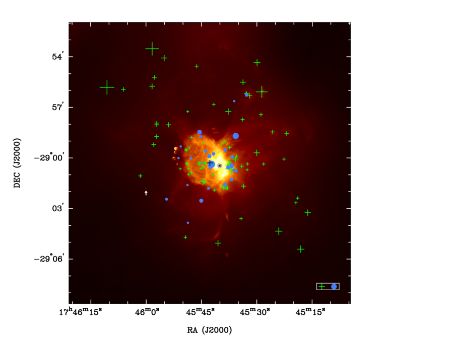
Figure 1: The 5-GHz image of the radio bright zone (RBZ), constructed with hybrid data obtained from a combination of observations with the JVLA in the A, B and C arrays, the old VLA in D array, and the GBT in single-dish mode, giving good uv coverage between 0 and 800 k$\lambda$. The RMS noise is $\sim$2 $\mu$Jy beam^-1. The synthesized FWHM beam is 0.68”x0.47” (8.4^o). The green cross symbols, ”+”, mark the positions of the radio variables and transients (N=82) and the blue dots indicate the locations of non-variables (N=28). These GCCR sources are newly identified from the JVLA high-resolution images observed at 5.5 GHz in A-array during 2014 May and 2019 September. A total of 118 compact sources are located outside Sgr A West and the HII regions A, B, C, D in Goss et al. (1985) or G-0.02-0.07 in Mills et al. (2011). The size of the symbols is scaled as $\sim 10"{\left[S/1\leavevmode\nobreak\ {\rm mJy}\right]}^{1/3}$, where $S$ is the source flux density. The size of the symbols in the box at bottom-right corresponds to a 1 mJy source for both variables (”+”) and non-variables (dot). The Galactic plane is oriented in this figure at a position angle of $\sim 30^{\rm o}$. A white arrow marks the location of the nebular source G-0.04-0.12 (see Figure 2 for details). The black ”+” marks the phase center of the data or the pointing center of the observations; the coordinates of the phase center are given in the footnote³ in the text. The black 16-pointed star marks the position of Sgr A*.

Figure 2: The 5.5-GHz images of the nebular source G-0.04-0.12 (Mills et al., 2011) produced by filtering out the short-spacing uv data at the three epoch’s observations at 2019-9-8 (left), 2014-5-26 (middle) and 2014-5-17 (right) and applying the correction for PB attenuation. The dirty images were cleaned with the MS-MSF algorithm (Rau & Cornwell, 2011) and the images with cleaned components were finally convolved with a common beam of FWHM 0.50”$\times$0.24” ($-0.05^{\rm o}$) instead of their synthesized beams. The intensities of the source observed at the three epochs can be compared without bias. Then, the difference between the levels of background emission caused by the different HA coverages of the data are correctable in the measurements of flux density (see Section 2.2.3). The total flux density of an extended source can be determined reliably in all epochs. The contours are 1$\sigma\times$(10, 11, 13, 16, 20, 25, 31, 38, 46, 55, 65), where the local RMS noise $\sigma=$10$\mu$Jy beam^-1. The integrated flux densities of 14.8$\pm$0.3, 14.6$\pm$0.3, and 14.7$\pm$0.3 mJy are determined for the epochs 2019-9-8, 2014-5-26 and 2014-5-17, respectively. The source G-0.04-0.12 is marked with a white arrow in the wide field image (Figure 1), located at a distance of 3.5 arcmin from the field center, close to the contour at the half power beam width (HPBW).

2.2 Imaging

Following the procedure for high dynamic range (DR) imaging that we developed recently (Zhao, Morris & Goss, 2019) and applying it to the Sgr A data with CASA, we have produced a deep image of the GC RBZ at 5.5 GHz with hybrid data obtained from a combination of observations with the JVLA in the A, B and C-arrays, the old VLA in D-array and the GBT in single-dish mode, providing good uv coverage between 0 and 800 k$\lambda$ (see the background image in Figure 1). The RMS noise in a region far from the bright emission region Sgr A West is 2 $\mu$Jy beam^-1. The ratio of the peak intensity, 0.8 Jy beam^-1, to the value of the RMS noise implies a DR of 400,000:1. Indeed, the rms noise is similar to the mean 5.5 GHz flux density of MSPs at the Galactic center, as extrapolated from the 1.5 GHz value assuming a frequency dependence of $\sim\nu^{-1.7}$.

However, the Sgr A West region that hosts the nuclear star cluster emits a diffuse continuum with a total flux density of $\sim$ 15 Jy at 5 GHz, distributed in the circumnuclear disk (CND), in addition to the prominent mini-spiral feature (Ekers et al., 1983). The confidence level for detections of weak compact sources near a strong radio complex may be compromised because of various issues in sampling and imaging radio interferometer array data. In a study of compact sources lying within a large field covered by a single primary beam (PB), both PB attenuation and smearing effects due to both bandwidth- and time-averaging can produce a loss in intensity of a compact source. Corrections must be applied for the errors caused by these effects.

2.2.1 Contamination from short-spacing power

High-amplitude short-spacing visibilities produce confusion due to the corresponding extended emission. In particular, an extended structure sampled by short baselines in high resolution imaging can emerge from the analysis of several small clumps that potentially lead to confusion in the identifications of weak compact sources. In addition, the relatively weak emission from compact radio sources is easily hidden in a bright extended emission complex, such as the Sgr A complex (see Figure 1). The high radio power at the Galactic center may explain why only a few bright compact sources in the RBZ have so far been reported. Furthermore, owing to limitations of the available deconvolution algorithms, false compact sources may be produced by residual sidelobes of a dirty beam near a strong extended emission region. For example, the FT of a uniform disk is a 2D Airy function. A dirty image of a VLA sampled disk source is difficult to clean because of strong sidelobes and residual phase errors (e.g., Ledlow et al., 1992). To quantitatively evaluate the contamination from residual sidelobes of a disk source, we carried out simulations with CASA processing of visibility models using the same procedure as utilized for the real data. Three visibility data sets for a model of the diffuse disk of Sgr A West (75”$\times$40”, PA=0^o) were made, corresponding to the uv coverages sampled in each of the three epochs’ observations (Table 1). We cleaned the sidelobes of the disk model with the CASA task TCLEAN, and noticed that compact clumps present outside the disk do mimic compact radio sources up to an intensity of 0.2 mJy beam^-1. These compact clumps are the sidelobes of the discrete sampling function simulated for the disk model, but appear as discrete radio sources due to the limitation in the clean process for a disk of emission. The limitation of handling the sidelobes from a complex emission source can therefore produce false compact sources.

One way to resolve this issue is to process the imaging with a cut-off of the short-baseline data that corresponds to extended emission. With the VLA A-array data at 5.5 GHz, we find that using only the longer baseline ($>100\leavevmode\nobreak\ k\lambda$) data, corresponding to sampling the small scale ($<2$ arcsec) emission, work well for diminishing the level of the residual sidelobes. Following the same procedure described above, we cleaned the disk model with lower baseline cutoff of 100 k$\lambda$. The RMS outside the disk in the cleaned image is improved by a factor of 15 as compared to that with all the A-array data; the maximum of the surrounding clumps drops by a factor of 100, and the RMS is reduced to a level of 1 $\mu$Jy beam^-1.

This algorithm has been applied to the real data. With the three A-array data sets, we constructed images having 20k$\times$20k pixels covering the 15’$\times$15’ of the RBZ region using only the longer baseline uv data ($>100\leavevmode\nobreak\ k\lambda$). The properties of the high-resolution images at the three epochs are summarized in columns 8-10 of Table 1. A nebular source G-0.04-0.12 (Figure 2) with a size of 3”$\times$4”, presumably with a constant flux density, is located southeast of Sgr A East (Mills et al., 2011). After filtering out the short baseline data, the resultant image is used to verify the consistency of the flux-density scale using our method. The images made from the longer baseline data ($>100\leavevmode\nobreak\ k\lambda$) at the three epochs show a nearly identical ring of the nebula, demonstrating consistent images obtained with the algorithm discussed here. We find no suspected arifacts surrounding the nebular ring in the cleaned images down to a level of 10 $\sigma$.

2.2.2 PB-corrections and uncertainty

With the sensitivity of the JVLA, we are able to detect a compact source at a large radial distance from the telescope pointing center. In a region far from the telescope pointing center, the uncertainty in the correction for attenuation becomes large. We carried out PB corrections with AIPS task PBCOR using a polynomial model updated by Perley (2016):

$$\centering A(x)=\sum_{i=0}^{i=3}A_{2i}x^{2i}\@add@centering$$ (1)

with a variable $x=\nu r$, where $\nu$ is the observing frequency and $r$ is the angular distance from the PB center, and $A_{2i}$ is the polynomial coefficients used in fitting the VLA PB. We corrected the image to the 2% level of the PB. At a large distance from the PB center, the corrections are subject to an increased uncertainty. The uncertainty $\sigma_{A}$ of $A(x)$ can be assessed with the formula:

$$\centering\sigma_{A}=\sqrt{\sum_{i=0}^{i=3}\Big{(}\frac{\partial A(x)}{\partial A_{2i}}\sigma_{A_{2i}}\Big{)}^{2}},\@add@centering$$ (2)

where $\sigma_{A_{2i}}$ are the uncertainties in the polynomial coefficients $A_{0}$, $A_{2}$, $A_{4}$ and $A_{6}$ given in Perley (2016).

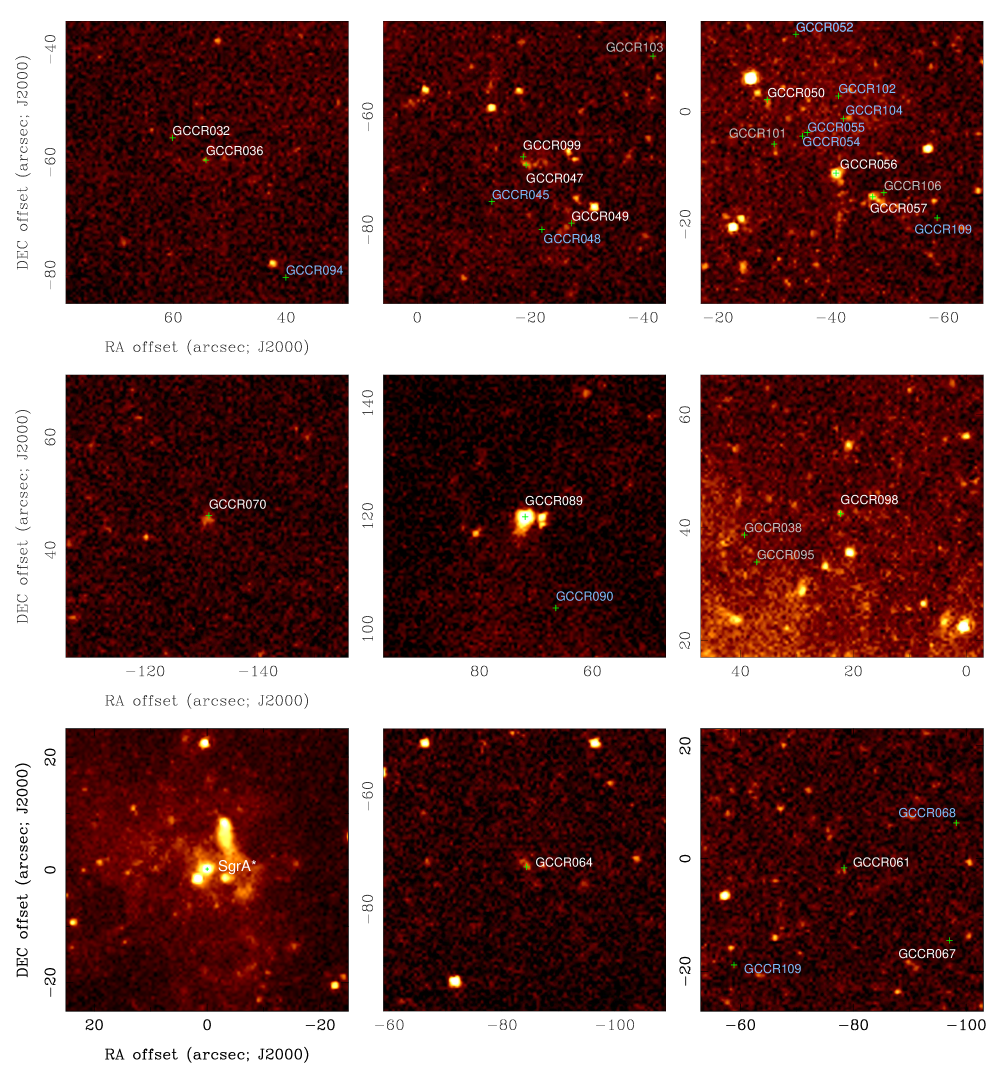
Figure 3: X-ray images showing the X-ray counterparts to the cores of the selected GCCR soures. The background X-ray image, from Zhu et al. (2018), has a spatial resolution of 0.5”. The ”+” symbols mark the positions of the GCCR sources. The bottom-left panel is the field including Sgr A* and the central panel is the field including the X-ray cannonball (GCCR089). Sgr A* and the cannnonball are both compact and bright in X-rays and radio, and these two compact sources were used to align the coordinate frames between the X-ray and radio images. The coordinates on all nine fields are the angular offsets in RA and Dec from Sgr A*. The colors represent the angular offsets between a GCCR and its possible X-ray counterpart in the ranges of $<1"$ (white), $1"-2"$ (grey), and $>2"$ (light blue), corresponding to identification code ”y”, ”y?” and ”n” marked in column 13 of Table 2.

2.2.3 Hour-angle vs. variation of flux density

The variability in flux density is one of the properties that facilitates differentiating between various types of compact radio sources (e.g., Kramer et al., 2006; Brook, et al., 2018; Coriat et al., 2011). Often, a compact radio source is associated with an extended emission feature surrounding an unresolved core. In such cases, the combination of intrinsic structure of a source and HA-range in uv sampling may produce a false variability. To access the uncertainty introduced by such an effect, we simulated a linear source described by a 2D Gaussian function (0.8”$\times$0.1”, 0^o or 90^o ) of 0.5 mJy by adding an unresolved core, or a point source, of 0.1 mJy at the center of the linear source. With two intrinsic PA values of 0^o and 90^o for the linear components, ten models of simulated linear+core source were distributed at ten positions at radial distances of up to 2 arcmin from the phase center to simulate three data sets. The simulated uv data sets were made by sampling the source models in the A-array configuration with HA-coverage identical to the real data, producing 128 channels covering a 2 GHz bandwidth at 5.5 GHz. Then, following the same setup and procedure as used to process the real data, the simulated data sets were Fourier-transformed by averaging every 2 channels, with the lower uv cutoff of $100$ k$\lambda$; and the dirty images were cleaned with CASA programs. With the AIPS task JMFIT, we made a Gaussian fit to the model sources found in the cleaned images, and find that the loss in flux density is in the range between 2%-10% of the input values for the extended linear feature. The loss in peak intensity is larger for the point source, or the core, falling in the range between 30% to 65% of the input values due to the bandwidth smearing (BWS) effect. The loss in peak intensity of the cores due to the BWS effect is correctable with JMFIT. For example, the correction factor $\sqrt{1+\beta^{2}}$ can be computed, where $\beta$ is provided in Eq(A4) of Appendix A.

The images of the nebula G-0.04-0.12 at three epochs made with three A-array data sets (Figure 2) were used to examine the issues of flux-density variation caused by changes of HA coverage. The difference in HA coverage between the three epochs’ observations does cause a minor difference in the level of a shallow negative hole underlying and surrounding an extended emission feature although the same uv cutoff ($>100$ k$\lambda$) was consistently applied. The apparent flux densities from the positive HA images (2019-9-8 and 2014-5-26 of Figure 2) agree well with each other while the apparent flux density derived from the 2014-5-17 image corresponding to the data taken with a negative HA-coverage decreases significantly due to a relatively deeper shallow negative area surrounding the source. The apparent flux densities integrated over the source are 14.6$\pm$0.2 mJy, 14.5$\pm$0.2 mJy and 11.3$\pm$0.20 mJy determined from the images of 2019-9-8, 2014-5-26, and 2014-5-17, respectively. The corresponding values of the flux density contributed from the shallow negative hole underlying the source are $-0.2\pm$0.2 mJy, $-0.1\pm$0.2 mJy, and $-3.4\pm 0.2$ mJy. The zero or background level biased by the HA coverage in the flux-density measurements can be corrected by simply subtracting the negative flux density from the apparent source flux density. After corrections for the local negative level, the variation in the final reported flux densities of 14.8$\pm$0.3 mJy, 14.6$\pm$0.3 mJy and 14.7$\pm$0.3 mJy at the three epochs for the nebula are consistent with the RMS fluctuations at a level of less than 2%, similar to the uncertainties propagated from the flux-density calibrations. In summary, the analysis of the nebular data verifies that a signficant difference in the zero level surrounding a source is potentially present due to differences in HA coverage for the uv data, but the bias in the determination of source flux density with Gaussian fitting is correctable with subtraction of a fitted background level using the AIPS task JMFIT automatically. Our examinations of G-0.04-0.12 images provide the procedure used for reliable measurements of the compact sources that are discussed in the rest of the paper.

Finally, we assessed a possible loss in source intensity caused by time-average smearing (TAS), using a model of circular uv-coverage with Gaussian tapering (Bridle & Schwab, 1999). We find that the fractional losses due to TAS for the sources listed in Table 2 are less than 2% in general. For the sources located within the HPBW of the PB, the loss is less than 0.5%. Therefore, no corrections for the effect of TAS have been applied.

3 Catalog of compact radio sources

A population of compact radio sources within the RBZ – at a level down to tens of $\mu$Jy – has been revealed with our 5.5 GHz VLA observations (Zhao, Morris & Goss, 2020). The sub-mJy compact radio sources are thought to consist of a mixture of thermal sources associated with compact/ultra-compact HII regions and non-thermal synchrotron sources that are related to the particle acceleration occuring in the accretion process associated with closely interacting binary stars or perhaps with isolated pulsars and PWNs. In this paper, we primarily searched for the GCCRs outside of the known HII regions. From the VLA A-array images observed in the three epochs, we have identified 110 compact sources located outside Sgr A West and the Sgr A East HII regions, G-0.02-0.07, but within a radius of $7.5^{\prime}$ from the pointing center of the observations. The search criteria for the GCCRs are based on their compactness (a size of $\theta_{\rm maj}<1$”) and significance ($S/\sigma>10$).

Appendix A discusses the GCCR catalog (Table 2) in detail, along with the presentation of high-resolution images of every GCCR source at 5.5 GHz (Figure A1).

4 X-ray counterparts

4.1 Catalogs of X-ray sources and Chandra images

Catalogs of X-ray sources in the region surrounding the Galactic center have been produced using data from the Chandra X-Ray Observatory by combining observations taken on many different occasions (Muno et al., 2003, 2006, 2009; Zhu et al., 2018). The central Chandra pointing with the ACIS-I detector covers an area of 17’$\times$17’, which is comparable to the primary beam of the JVLA at 5.5 GHz. The Chandra field overlaps strongly with our JVLA field of view. We therefore cross-correlated our GCCR catalog with the ultra-deep point-source X-ray catalog of Zhu et al. (2018), which incorporates Chandra observations between 1999 and 2013, and reports 3619 sources in the 2-8 keV band within 500” of Sgr A*. For regions outside the Zhu et al. (2018) catalog area, we used earlier catalogs covering a greater area (Muno et al., 2008, 2009) for the cross-correlation analysis.

For candidate X-ray counterparts to GCCR sources, we also carried out a careful examination of the X-ray image used by Zhu et al. (2018) to construct their catalog. The two previously known compact X-ray and radio sources — Sgr A* and the Cannonball — were used to align the coordinate frames of the X-ray and radio images. The reference centers of both images were shifted to the position of Sgr A*: RA(J2000) = 17:45:40.0409, Dec(J2000)= -29:00:28.118. The precision in the positional alignment between the Chandra X-ray and JVLA images is $\sim 0.25(S/\sigma)^{-1}$ arcsec ($<0.1$ arcsec), where ${S}/{\sigma}$ is the ratio of signal to noise for the reference sources used in the alignment. We found candidates using the catalog cross-correlation, and then used the images to verify the coincidence and to look for possible structure in the X-ray morphology that might be helpful in assessing the correspondence. Figure 3 plots examples of those possible X-ray counterparts in 50”$\times$50” sub-frames used in the identification process. We examined as well the three Chandra images in the 2-3.3, 3.3-4.7 and 4.7-8 keV bands for the central 900” that fully cover the RBZ observed at 5.5 GHz for the distribution of the GCCRs. Thus, the cross-correlation analysis between X-ray and 5.5 GHz radio is spatially complete. Identifications of X-ray counterparts to individual GCCRs are tabulated in Table 3. Column 1 is the GCCR-ID. Column 2 lists the name of an X-ray source in the Chandra X-ray Observatory catalog, CXOGC#, where # stands for truncated J2000 coordinates of the source JHHMMSS.S-DDMMSS (Muno et al., 2009). In the diffuse X-ray source catalog of Muno et al. (2008), the name of an X-ray source is denoted as G# where # stands for DDD.DDD$\pm$D.DDD, the Galactic coordinates in degrees. Column 3 gives the source sequential numbers (SS#) in the deep X-ray catalog of Zhu et al. (2018). Column 4 gives the angular offsets between the GCCRs and their X-ray counterparts. Column 5 lists the 2-8 keV photon flux ($S_{\rm 2-8\leavevmode\nobreak\ keV}$) reported in the catalogs, or the range of reported fluxes (upper — lower values) (Muno et al., 2008, 2009; Zhu et al., 2018). Column 6 gives the references from which the X-ray data are used in the identifications.

Table 3: Identifications of candidate X-ray counterparts of GCCRs

GCCR-ID	CXOGC# or G#	SS#	$\Delta\theta_{\rm X-R}$	$S_{\rm 2-8\leavevmode\nobreak\ keV}$	Ref.‡
			(arcsec)	(10-7 ph cm-2 s-1)
(1)	(2)	(3)	(4)	(5)	(6)
GCCR001	J174610.5-285550	…	1.5	60	a
GCCR004	J174558.4-285546	…	1.2	3.6	a
GCCR014	J174549.3-290442	…	0.6	5.8	a
GCCR015	J174549.3-290442	…	0.5	5.8	a
GCCR031	J174544.9-290017	…	0.8	5.5	a
GCCR032	…	2625	0.2	2.8	b
GCCR035	J174544.2-290018	…	0.7	7.5	a
GCCR036	J174544.1-290128	2594	0.5	4.5	a,b
GCCR037	J174543.9-290020	…	1.5	15	a
GCCR038	…	2502	2	2.1	b
GCCR041	J174541.5-285651	…	1.8	1.7	a
GCCR047	G359.925-0.051	…	…	18.1	c
GCCR049	…	1898	1	8.12 — 7.50	b
GCCR050	…	1875	1	7.4 — 5.6	b
GCCR056	J174536.9-290039	1767	0.2	43.0 — 42.2	a,b
GCCR057	G359.933-0.037	…	…	22.8	c
GCCR058	G359.941-0.029	…	…	18.7	c
GCCR059	J174535.6-285953	1617	1.6	6.44 — 3.60	a,b
GCCR061	J174534.0-290030	1429	0.8	4.96 — 4.80	a,b
GCCR064	J174533.5-290140	1375	0.4	9.10 — 6.17	a,b
GCCR067	J174532.6-290043	1250	1	1.28 — 1.20	a,b
GCCR070	J174530.0-285942	956	0.7	17.5 — 17.0	a,b
GCCR072	J174528.8-285726	852	0.4	4.1 — 3.5	a,b
GCCR073	J174528.6-285605	819	0.8	9.6 — 8.7	a,b
GCCR074	J174528.1-290021	774	1	3.34 — 1.50	a,b
GCCR077	…	389	1	1.12	b
GCCR082	J174516.1-290315	185	0.6	40.3 — 30.0	a,b
GCCR085	J174550.6-285919	3042	0.3	3.2 — 1.7	a,b
GCCR087	J174548.7-290350	2926	0.4	3.2 — 2.4	a,b
GCCR089	J174545.5-285828	…	0.3	170	d,a
GCCR092	J174544.6-290020	…	2	2.7	a
GCCR095	…	2477	1.9	4.23	b
GCCR096	J174542.5-290033	…	1.2	1.9	a
GCCR097	J174542.2-290024	…	1.9	3.1	a
GCCR098	J174541.7-285945	2369	0.2	6.80 — 6.63	a
GCCR099	G359.925-0.051	…	…	18.1	a
GCCR100	J174538.6-285933	…	2	1.2	a
GCCR101	J174537.6-290035	1857	1.6	10 — 6.0	a,b
GCCR103	J174536.8-290117	…	0.4	1.5	a
GCCR106	G359.933-0.037	…	…	22.8	c
GCCR107	J174536.1-285638	1671	0.5	190 — 186	a,b
GCCR110	J174532.7-285617	1263	0.7	9.4 — 6.9	a,b

^‡References: a. Muno et al. (2009); b. Zhu et al. (2018), c. Muno et al. (2008); and d. Park et al. (2005).

In addition, notes for those GGCRs involving extended X-ray emission sources such as halos and elongated nebulae, or possessing possible IR identifications, are given in Section 4.2.

In short, a total of 42 GCCRs have candidate X-ray counterparts; most of them (27) have a positional offset between X-ray and radio, $\Delta\theta_{\rm X-R}$, less than 1” or less than twice the Chandra resolution; the rest of them (15) have $\Delta\theta_{\rm X-R}=$1” to 2”. The probability that a GCCR source has an accidental coincidence within 1” or 2”, given the number of $\sim$3900 reported X-ray sources (Muno et al., 2009; Zhu et al., 2018) lying within the area covered by our radio survey, is 1.9% or 7.7%, respectively. Thus, most of the 42 GCCRs with candidate X-ray counterparts are likely related to the X-ray sources. The majority of the GCCRs (68) do not have X-ray counterparts within 2 arcsec. The presence or absence of a candidate X-ray identification for the indvidual GCCRs is also indicated in Table 2 in the Appendix.

4.2 Notes to the X-ray counterparts

${\bf GCCR001}\leavevmode\nobreak\ -$ CXOGC J174610.5-285550 (Muno et al., 2009), is offset by 1.5” from the radio source. An extended X-ray halo of size 15” surrounds the compact X-ray source in the 2.0-3.3 keV and 3.3-4.7 keV bands, but no significant X-ray emission is present in the 4.7-8 keV band.

${\bf GCCR047}\leavevmode\nobreak\ -$ This radio source is associated with a bright spot in an X-ray complex, see the top-middle panel in Figure 3. The X-ray source is listed in Muno et al. (2008) as G359.925-0.051 with a power-law spectrum of $\Gamma=1.77$ and X-ray luminosity of 3$\times 10^{32}$ erg s^-1; it is one of the twenty PWN candidates within the central 20 pc (Muno et al., 2008).

${\bf GCCR056}\leavevmode\nobreak\ -$ CXOGC J174536.9-290039 (Muno et al., 2009), is a compact X-ray source having an offset ¡0.2” from the radio source. In the deep X-ray catalog of Zhu et al. (2018), this source is listed as SS#1767. The deep X-ray image shows that the bright compact X-ray source appears to be at the end of a long (25”) and slightly curved filament that extends to south (see the top-right panel of Figure 3). The compact radio source GCCR056 is embedded in extended radio source M which also has a filamentary component (Yusef-Zadeh & Morris, 1987), but the long ($\sim$20”) radio filament is oriented toward the northwest (Zhao, Morris & Goss, 2016), so that the angle between the X-ray and radio filaments is about 120^o.

${\bf GCCR057}\leavevmode\nobreak\ -$ This source, located 3” SW of GCCR056, coincides with a compact X-ray source at the tip of a linear feature that appears only in the Muno et al. (2008) catalog of extended X-ray sources; see the top-right panel of Figure 3. The linear X-ray source, G359.933-0.037, has a power-law spectrum of $\Gamma=1.59$ and an X-ray luminosity of 3$\times 10^{32}$ erg s^-1, which is one of the twenty suggested PWNs within the central 20 pc (Muno et al., 2008).

${\bf GCCR058}\leavevmode\nobreak\ -$ The radio source appears to be associated with a compact X-ray source sunrounded by extended emission source, G359.941-0.029 (Muno et al., 2008). The authors report a power-law spectrum of $\Gamma=0.44$ and an X-ray luminosity of 2$\times 10^{32}$ erg s^-1. The X-ray source is one of the twenty suggested PWNs within the central 20 pc (Muno et al., 2008).

${\bf GCCR070}\leavevmode\nobreak\ -$ The X-ray counterpart CXOGC J174530.0-285942 (Muno et al., 2009), which is offset by 0.7” from the radio source and is also found in Zhu et al. (2018) as SS#956. The deep Chandra image shows the X-ray source having an amorphous halo with a size of $\sim 4$” (see middle-left panel of Figure 3).

${\bf GCCR072}\leavevmode\nobreak\ -$ The X-ray counterpart CXOGC J174528.8-285726 (Muno et al., 2009), offset by ¡0.4” from the radio source, is also listed as SS#852 in the X-ray catalog of Zhu et al. (2018). The system is interpreted as an O-star in a colliding-wind binary (CWBs) or HMXB based on IR spectrocospy (DeWitt et al., 2013).

${\bf GCCR089}\leavevmode\nobreak\ -$ The X-ray counterpart CXOGC J174545.5-285828 (Muno et al., 2009). The compact X-ray source is associated with an extended X-ray source that is interpreted as a PWN (Park et al., 2005). See the central panel of Figure 3. The radio emission from the PWN was described by Zhao, Morris & Goss (2013). The compact source in both X-ray and radio likely emanates from near the neutron star (Park et al., 2005; Zhao, Morris & Goss, 2013).

${\bf GCCR099}\leavevmode\nobreak\ -$ This radio source may be associated with a faint X-ray component in the diffuse X-ray source, G359.925-0.051 (see the top-middel panel in Figure 3). It is interpreted as a PWN (Muno et al., 2008). It is located $\sim$1” NE of GCCR047 (see Figure A1 and Figure 3).

${\bf GCCR106}\leavevmode\nobreak\ -$ This source is located 2” NW of GCCR057, and may be also associated with the candidate PWN, G359.933-0.037 (Muno et al., 2008). See upper-right panel of Figure 3.

${\bf GCCR107}\leavevmode\nobreak\ -$ This source coincides (with an offset ¡0.5”) with the X-ray source CXOGC J174536.1-285638 / SS#1671 (Muno et al., 2009; Zhu et al., 2018). An investigation of the X-ray observations of the compact X-ray source implies an apparent 189$\pm$6 day periodicity present in the lightcurve (Mikles et al., 2008). The system is likely associated with an HMXB (Mikles et al., 2008) or with a colliding wind binary based on its IR spectrum (Clark et al., 2009). A spectral type of WN8-9h is suggested for the donor star (Mauerhan et al., 2010).

${\bf GCCR110}\leavevmode\nobreak\ -$ The X-ray counterpart CXOGC J174532.7-285617 / SS#1263 (Mauerhan et al., 2010; Zhu et al., 2018) is offset by ¡0.7” from the compact radio source. Near infrared spectroscopy implies that the system is associated with a spectral type O4-6I star Mauerhan et al. (2010).

5 Astrophysical implications

5.1 Spatial distribution & extragalactic contribution

The GCCR sources appear to be mainly distributed along the Galactic plane (Figure 1), indicating that a significant fraction of the compact radio sources are located in the RBZ at the Galactic center. However, at the tens of $\mu$Jy level, the density of background extragalactic radio sources becomes noticeable. For example, the VLA deep observations at 5 GHz of the Great Observatories Origins Deep Survey - North (GOODS-N) ($\sigma_{\rm RMS}$=3.5 $\mu$Jy beam^-1, synthesized beam of 1.47”$\times$1.42”) and GOODS-S ($\sigma_{\rm RMS}$=3.0 $\mu$Jy beam^-1, with a beam of 0.98”$\times$0.45”) fields found that these two fields contain 52 and 88 sources over areas of 109 and 190 arcmin², respectively (Gim et al., 2019). The average source density in these two fields above a flux density of 15 $\mu$Jy is therefore $\sim$0.5 sources arcmin^-2.

From Table 2, a total of 83 GCCR sources is found in a 45 arcmin² region within the HPBW of the primary beam, excluding the area of 3 arcmin² covered by the Sgr A West and Sgr A East HII regions. The density of GCCR sources above the 70 $\mu$Jy cutoff is therefore $\sim$1.8 sources arcmin^-2. If we use our GCCR cutoff of 70 $\mu$Jy to re-count the sources listed in the GOODS-N and -S catalog (Gim et al., 2019), the number of sources in the GOODS-N and -S surveys drops to 46, lowering the source density to 0.15 sources arcmin^-2. Therefore, the density of GCCRs revealed by our search is an order of magnitude higher than that found in the GOODS-N and -S fields.

We note that the extragalactic source density of 0.15 sources arcmin^-2 at 5 GHz derived from the GOODS-N and -S fields is consistent with that of $\sim$0.1 sources arcmin^-2 for extragalactic background sources above 100 $\mu$Jy at 3 GHz based on the derived source density by Condon et al. (2012). Of course, the extragalactic background contribution is a function of the distance from the pointing center, for a given flux-density cutoff, because it takes a stronger source to appear above the limit out at the edge of RBZ. In conclusion, we find that, at most, about 10% of the GCCR sources are expected to be associated with the extragalactic background population.

5.2 Flux density distribution & cataclysmic variables

The Galactic center hosts a large population of cataclysmic variables that are associated with hard X-ray sources (e.g. Muno et al., 2004). In a recent JVLA survey for radio emission from CVs, Barrett et al. (2017, 2020) reported new detections of 33 magnetic CVs, or mCVs, with flux density in the range from 6 to 8031 $\mu$Jy at frequencies ranging between 4.5 and 22.1 GHz, increasing the number of radio sources associated with CVs to 40. The radio emission of the mCVs is circularly polarized (Barrett et al., 2020) with relatively flat spectra (Barrett et al., 2017). Most of the radio CVs are nearby, at distances ranging from 88 pc to 2.24 kpc, spanning a radio luminosity range from 3$\times 10^{24}$ erg s^-1 to 1.7$\times 10^{27}$ erg s^-1.

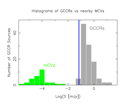
Figure 4: Flux-density distributions of GCCRs (grey) versus the 33 nearby mCVs (green) detected with the VLA (Barrett et al., 2020). The flux densities of the mCVs in this histogram are from JVLA observations at frequencies between 4.5 and 22.1 GHz, extrapolated to the GC at D=8 kpc assuming a flat spectrum with $\alpha=0$. The blue vertical line marks the flux-density cutoff for GCCRs, 70 $\mu$Jy.

To compare the flux-density distribution of the radio CVs with our GCCRs, we scaled the radio flux density of CVs to the Galactic center by multiplying by ${\rm(D/8\leavevmode\nobreak\ kpc)}^{2}$. Figure 4 shows a histogram of the radio source counts as a function of radio flux density in the logarithmic range between $-5.8$ and 1.8, corresponding to a range of flux density between 1.6 nJy (10^-6 mJy) and 63 mJy at a distance of 8 kpc; the logarithm of flux density, Log(S [mJy]), is binned into $\Delta$ Log$(S[{\rm mJy}])=0.4$ intervals starting from $-5.8$ (1.6 nJy).

The grey histogram in Figures 4 and 5 shows a peak of 47 GCCRs between $-$1 to $-$0.6 in log (S [mJy]). No overlap in flux density is found between the population of detected mCVs (green) and our reported sample of GCCRs (grey).

The source counts below $-$1 (100$\mu$Jy) appear to be incomplete because only a small fraction of the GCCR candidates in the Log(S[mJy]) = -1.2 bin lie above our 70 $\mu$Jy cutoff marked by the blue vertical line in Figure 4. In spite of the cutoff, the logarithmic flux-density distribution of the GCCR population shows a large dispersion, with an average of $\mu_{\rm Log(S[mJy])}=-0.44$ and an RMS of $\sigma_{\rm Log(S[mJy])}=0.47$. The high-intensity tail of the distribution suggests that the distribution of GCCRs may consist of multiple Gaussian or normal distributions of different source types. However, we can not rule out the possibility that the GCCR population shows an abnormal distribution of the compact radio sources.

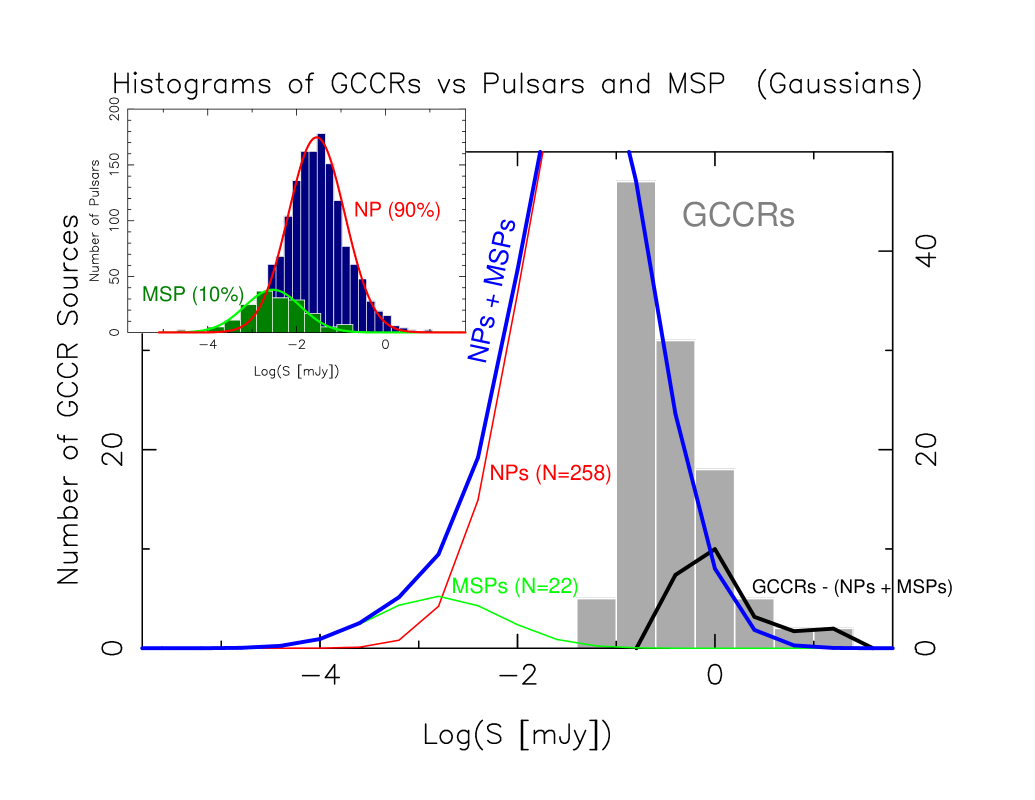
Figure 5: The flux-density distribution of GCCRs (grey histogram) is fitted with a sample of 258 NPs (red Gaussian curve) and 22 MSPs (green Gaussian curve), a 70% of the Galactic disk (GD) NPs and MSPs sample used in Kramer et al. (1998). The blue curve is the sum of the two Gaussians. The black curve denotes the difference between counts of the GCCR distribution (grey histogram) and of the distrbution (the blue curve) that is extrapolated from the population of NPs and MSPs in the Galactic disk. The 1.5 GHz flux densities of the NPs and MSPs from the samples of Kramer et al. (1998) have been scaled to the flux densities at 5.5 GHz assuming $\alpha=-1.7$. The Kramer et al. (1998) sample has also been scaled to the Galactic center distance by scaling their flux densities by ${\rm[1\leavevmode\nobreak\ kpc/8\leavevmode\nobreak\ kpc]}^{2}$. The top-left inset shows the distributions of 1503 NPs (dark blue histogram) and 169 MSPs (dark green histogram) based on a large sample observed at 1.4 GHz (Manchester et al., 2005). The 1.4 GHz flux densities have also been scaled to the flux densities at 5.5 GHz in the Galactic center assuming $\alpha=-1.7$ and the GC distance of 8 kpc. The red (NPs) and green (MSPs) curves show the fitted Gaussian distributions with $\mu_{\rm NP}=-1.3$ and $\mu_{\rm MSP}=-2.5$ as well as a common standard deviation of $\sigma=0.64$.

5.3 Normal pulsars and MSPs at the Galactic center

We consider here the possibility that some of the GCCRs could be pulsars. While the present formation rate of massive stars in the GC is large enough to give rise to the expectation that pulsars would be abundant in the GC, very few are known, presumably because the foreground scatter broadening toward the GC (e.g., Spitler et al., 2014) leads in most cases to a sufficiently large pulse broadening that the pulses become indistinguishable. However, with sufficient sensitivity, pulsars can be detected as point-like continuum radio sources or as pulsar wind nebulae.

A comparison of luminosities and spectral indices between samples of normal pulsars (NP) and millisecond pulsars (MSP) has been conducted by Kramer et al. (1998) based on 31 MSPs and 369 NPs distributed in the Galactic disk (GD) (Also see Lorimer et al., 1995; Taylor et al., 1993). They showed that NPs and MSPs have similar spectra, with spectral indices of $\alpha=-1.6\pm 0.04$ and $\alpha=-1.8\pm 0.1$, respectively. In addition, the MSPs are an order of magnitude less luminous than NPs. A mean value of Log(Sd² [mJy kpc²]), $\mu_{\rm MSP}=0.5\pm$0.2 at $\sim$1.5 GHz, is derived for MSPs as compared to $\mu_{\rm NP}=1.5\pm$0.04 for the NPs (Kramer et al., 1998). As noted by Kramer et al. (1998), the statistics may be subject to a bias owing to the fact that most NPs were discovered in surveys at higher frequencies (that correspondingly selected flatter spectrum and more luminous pulsars), and that most MSPs were discovered at low frequencies and were therefore relatively nearby subject to limitations in dispersion removal. To avoid possible statistical bias caused by the difference in the observed luminosities of MSPs and NPs, Kramer et al. (1998) investigated a statistically complete sample of nearby MSPs and NPs. They demonstrated that the discrepancy of the mean values between MSPs and NPs becomes small in the case of restricting to a nearby population within a distance of $1.5$ kpc. They find that the mean values of $\mu_{\rm MSP}$ and $\mu_{\rm NP}$ are $0.0\pm$0.1 and $0.57\pm$0.09 at $\sim$1.5 GHz, respectively, in a nearby population of 18 MSPs and 55 NPs after removing the apparent biases.

However, the nearby sample excludes the high-luminosity NPs and MSPs that may make a significant contribution to the GCCR population. We would need a large number of pulsars ($\sim 3000$) to fit the upper tail of the GCCR distribution if we scaled the nearby sample of Kramer et al. (1998) to the Galactic center. The GD population appears to be more relevant to the distribution of GCCRs. Using the spectral index $\alpha=-1.7$ for both MSPs and NPs and a distance of 8 kpc for the Galactic center, we extrapolated the mean values of $\mu_{\rm MSP}$ and $\mu_{\rm NP}$ at 1.5 GHz of the GD population of MSPs and NPs to the corresponding values at 5.5 GHz for the GC population, giving $\mu_{\rm MSP}=-2.3$ (5$\mu$Jy) and $\mu_{\rm NP}=-$1.3 (50$\mu$Jy) at 5.5 GHz. We then compare the extrapolated GD populations of 369 NPs and 31 MSPs to the distribution of GCCRs in Figure 5, by approximating the pulsar distributions as Gaussian with a common standard deviation of $\sigma=0.64$; the value of $\sigma$ was estimated from the FWHM of the NPs’ distribution in Log(S$\rm d^{2}[{\rm mJy\leavevmode\nobreak\ kpc^{2}}])$ (Fig. 2 of Kramer et al. 1998). Therefore, on the tentative assumption that all the GCCRs in the 100-250 $\mu$Jy bin are pulsars, except for the 10% of them expected to be extragalactic sources, a total of 22 MSPs and 258 NPs would be needed to account for the GCCR distribution. Namely, 70% of the GD population, used in the Kramer et al. (1998) analysis, would be required to match the 47 GCCRs detected in the Log$(S[{\rm mJy}])=-1$ bin covering the flux density range 100-250 $\mu$Jy.

We further inspected and verified the statistics of Kramer et al. (1998) with a large sample of 1672 pulsars observed at 1.4 GHz (Manchester et al., 2005), 90% of which is NPs (spin period $P>30$ millisecond) and 10% is MSPs ($P\leq 30$ millisecond); see the inset of Figure 5. Scaling to the flux densities at 5.5 GHz at the Galactic center distance (D$=8$ kpc), and assuming $\alpha=-1.7$, we derive the mean ($\mu_{\rm NP}=-1.3$) and standard deviation ($\sigma=0.64$) of the logarithmic flux density from the 1503 NPs, that are in good agreement with the corresponding parameters derived from the GD sample of Kramer et al. (1998). The mean logarithmic flux density of MSPs ($\mu_{\rm MSP}=-2.5$) derived from the 169 MSPs is slightly less than the value ($\mu_{\rm MSP}=-2.3$) of the GD sample, indicating that a difference in the mean flux density between NPs and MSPs in the large sample is insignificantly greater than that of the GD sample.

Therefore, the analysis here is consistent with the possibility that up to 80% of the detected GCCRs could be NPs if the RBZ hosts a total of 280 NPs and MSPs with a distribution in radio luminosity similar to the GD distribution of NPs and MSPs. However, the MSP population essentially makes no contribution to the upper tail of GCCR sources detected in this paper. Of course, the possible number of NPs among the GCCRs given above is an upper limit, as other classes of sources can also contribute to the GCCR population, notably the X-ray binaries that we discuss below. A first filter for constraining the NP population among the GCCRs could be based on spectral index measurements, given the typically steep spectra of NPs ($\alpha\leavevmode\nobreak\ \sim\leavevmode\nobreak\ -1.7$). We also note that NPs are usually not strongly variable on time scales of 6 years or shorter (Paul Demorest, personal communication) and only 25% of the GCCRs are non-variable, so it appears that NPs are, at most, a minor fraction of the GCCRs. Of course, firmly identifying pulsars requires detection of their pulsed emission. To date, PSR J1745-2900 is the only confirmed pulsar within the RBZ. PSR J1745-2900 was first identified as an X-ray source by the Swift observatory during a flare (Kennea et al., 2013); and pulsed emission with a period of 3.76 s was revealed in follow-up observations by the NuSTAR observatory (Mori et al., 2013). We note that the analysis in this section does not cover the compact radio sources located within Sgr A West, and the Sgr A East HII complex. Located $\sim$3” away from Sgr A*, PSR J1745-2900 is not listed in Table 2, our GCCR catalog. The discovery of PSR J1745-2900, the GC magnetar, raises the possibility that it might be possible to detect pulsed emission from some of the GCCRs.

5.4 X-ray binaries

By comparing the GCCRs in our 5.5-GHz image with published catalogs of X-ray sources based on observations with the Chandra X-ray observatory, and with the Chandra X-ray image from Zhu et al. (2018), we find about 42 possible X-ray counterparts to the GCCRs (Figure 3). The GCCRs identified with X-ray counterparts could be close binary systems in which a compact stellar remnant accretes mass from its companion.

X-ray binaries can be divided into two major spectral states based on the hardness of their X-ray spectra: soft and hard states. The soft state is dominated by thermal emission from an accretion disk, while the hard state is dominated by the emission from the corona (Coriat et al., 2011). The radio emission in the hard state is usually characterized by a flat or slightly inverted spectrum with a spectral index of $\alpha\sim 0$, which can be interpreted as self-absorbed synchrotron emission from a compact jet, similar to those found in extragalactic nuclei (e.g., Blandford et al., 2019). During the soft state, the compact jets are likely to be quenched (e.g., Fender et al., 1999; Coriat et al., 2011). The presence of a strong correlation between radio and X-ray emission during the hard state has been investigated with observations of several X-ray binaries (e.g., Corbel et al., 2000; Migliari & Fender, 2006; Coriat et al., 2011; Tudor et al., 2017; Gallo et al., 2018; Qiao & Liu, 2019), showing a power-law relationship ($L_{\rm R}\propto\/L_{\rm X}^{\beta}$) between the luminosities of X-ray ($L_{\rm X}$) and radio ($L_{\rm R}$).

For black hole X-ray binaries (BHXB) (Fender et al., 2009), the standard value for the power-law index, $\beta\sim 0.6$ (Corbel et al., 2003, 2008; Gallo et al., 2003; Xue & Cui, 2007; Coriat et al., 2011) is thought to be related to the inner region of the accretion system where a hot and inefficient accretion flow (i.e., an advection-dominated accretion flow, or ADAF) might be present (Narayan & Yi, 1994; Narayan et al., 1997; Abramowicz & Fragile, 2013). The ADAF model appears to reasonably account for sources in the hard state while the radio emission is optically thick and is correlated with X-ray emission. On the other hand, a steady, powerful, relatively low bulk velocity or bulk Lorentz factor $\Gamma<2$ jet is always present in the hard X-ray state (Fender et al., 2009). The observed jets imply a combination of radiatively inefficient flows with the simultaneous presence of MHD winds or outflows. That is, advection-dominated inflow-outflow solutions, or ADIOS (Blandford & Begelman, 1999), may work for the BHXBs.

Similar power-law correlations between $L_{\rm X}$ and $L_{\rm R}$ are also shown by neutron-star X-ray binaries (NSXB), but BHXBs are more radio loud by a factor of 20-30 (Gallo et al., 2018; Kylafis et al., 2012). In a study of disk-jet coupling in low-luminosity accreting NSs in LMXBs, Tudor et al. (2017) show $L_{\rm R}\propto\/L_{\rm X}^{\beta}$ relations characteristic of three different types of NSs as compared to the standard relation $\beta\sim 0.6$ for BHXB. Transitional millisecond pulsars (tMSP) show $\beta\sim 0.6$, the same as that for BHXBs but with an order of magnitude less luminosity at 5-GHz than BHXBs. Non-pulsing NSs correspond to $\beta\sim 0.7$ while hard-state NSs have $\beta\sim 1.4$ (Tudor et al., 2017). It is worth mentioning that the data used in their analysis span six orders of magnitude in 5-GHz radio luminosity ($L_{\rm 5\leavevmode\nobreak\ GHz}:10^{25-31}$ erg s^-1) and nine orders of magnitude in the 1-10 keV X-ray luminosity ($L_{\rm X}:10^{30-39}$ erg s^-1.) The BHXBs are mainly distributed in the range of $L_{\rm 5\leavevmode\nobreak\ GHz}$: (10^28-31 erg s^-1) along the power-law correlation curve ($L_{\rm 5\leavevmode\nobreak\ GHz}\propto\/L_{\rm X}^{0.6}$), while the NSXBs are clustered in a domain around 10^27-29 erg s^-1 in $L_{\rm 5\leavevmode\nobreak\ GHz}$ and a few times 10^36-37 erg s^-1 in $L_{\rm X}$. For X-ray binaries having luminosities in the range of 10^36-37 erg s^-1, the BHXBs appear to be distinguishable from the counterpart NSXBs based on their much higher radio luminosities.

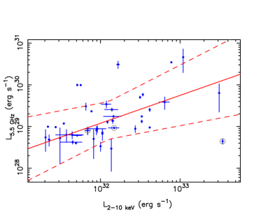
Figure 6: Plot showing the cross-correlation between X-ray and radio luminosities for the 42 GCCRs having X-ray counterparts. The radio luminosities are derived from the flux densities at 5.5 GHz given in this paper and the X-ray luminosities are derived from the X-ray photon fluxes in the 2-8 keV X-ray band reported in the X-ray catalogs (Muno et al., 2008, 2009; Zhu et al., 2018). The black circles mark the three candidate HMXBs (Section 4.2). The red solid line is the result from a least-squares fit to the logarithmic X-ray and radio luminosities, implying a power-law relation $L_{\rm 5.5\leavevmode\nobreak\ GHz}\propto L_{\rm 2-10\leavevmode\nobreak\ keV}^{\beta}$. The red dashed lines outline the range in which the true regression line lies at a confidence level of 95%, derived with Scheffé’s method, (https://en.wikipedia.org/wiki/Confidence_and_prediction_bands and https://www.itl.nist.gov/div898/handbook/prc/section4/prc472.htm).

We carried out a regression analysis for the cross-correlation between logarithmic radio and X-ray luminosities for the 42 GCCRs with X-ray counterparts. The radio luminosities are derived from the flux densities $S_{\nu}$ given in Table 2 using the form $L_{\nu}=4\pi D^{2}\nu S_{\nu}$ and $\nu=5.5$ GHz. The X-ray luminosities are derived from the photon flux values $S_{\rm 2-8\leavevmode\nobreak\ keV}$, listed in Table 2, provided in the Chandra X-ray catalogs (Zhu et al., 2018; Muno et al., 2009, 2008) using the form $L_{\rm 2-8\leavevmode\nobreak\ keV}=4\pi D^{2}S_{\rm 2-8\leavevmode\nobreak\ keV}f_{\rm 2-10\leavevmode\nobreak\ keV}$, where $f_{\rm 2-10\leavevmode\nobreak\ keV}$ is a photon flux-to-energy conversion factor. We adopted $f_{\rm 2-10\leavevmode\nobreak\ keV}=2.38\times 10^{-8}$ erg photon^-1 (Zhu et al., 2018) to compute the 2-10 keV unabsorbed energy flux. Figure 6 shows a plot of $L_{\rm 5.5\leavevmode\nobreak\ GHz}\leavevmode\nobreak\ vs.\leavevmode\nobreak\ L_{\rm 2-10\leavevmode\nobreak\ keV}$ for the 42 GCCRs with X-ray counterparts. We performed a least-squares regression analysis assuming a linear relationship between the logarithmic radio and X-ray luminosities, $\log\big{(}L_{\rm 5.5\leavevmode\nobreak\ GHz}{[\rm erg\leavevmode\nobreak\ s^{-1}]}\big{)}=\alpha+\beta\log\big{(}L_{\rm 2-10\leavevmode\nobreak\ keV}{[\rm erg\leavevmode\nobreak\ s^{-1}]}\big{)}$. We find that $\alpha=7.7\pm 0.45$ and $\beta=0.67\pm 0.02$ with a correlation coefficient R=0.72 and a probability of no correlation, P ¡ 0.01%. The $\beta$ value derived for the GCCRs appears to be consistent with the power-law relationships that are found for BHs, tMSPs, and non-pulsating NSs in the LMXB sample used in the analysis of Tudor et al. (2017).

We also note that the 5.5-GHz radio luminosities of the GCCRs with X-ray counterparts are in the luminosity range of 10^28-31 erg s^-1, consistent with the range of 5-GHz radio luminosities of the BHXBs used in the analysis of (Tudor et al., 2017). However, about twenty GCCRs with X-ray counterparts having 5.5-GHz radio luminosities below $1\times 10^{29}$ erg s^-1 could be explained as NSXBs. The five radio morphology types (given in column 12 of Table 2, Appendix A) of the GCCRs are also consistent with the possibility that the compact radio cores are produced from either BHXBs or NSXBs. If the compact cores of the GCCRs are associated with jet flows from the inner region of accretion disks or from the corona of compact objects, their radio spectra are expected to be flat (Coriat et al., 2011). In addition, a fraction of GCCRs associated with pulsars and MSPs discussed in Section 5.3 may belong to the catagory NSXBs, if they are binaries emitting X-rays. However, some of the GCCRs with X-ray counterparts listed in Table 3 may just be associated with PWNs powered by a single neutron star. Further study of the GCCRs with coordinated radio and X-ray observations will help to distinguish between BHs and NSs for the compact objects associated with the GCCRs.

Finally, we note that the recent detection of a 91$\pm 10$ $\mu$Jy source at 5.5 GHz at the position of the Galactic center transient caught during its flare in 1990 (GCT1990) with a flux density then of $\sim$1 Jy at 1.5 GHz (Zhao et al., 1992; Zhao, Morris & Goss, 2020), implying $L_{\rm 5.5\leavevmode\nobreak\ GHz}=2\times 10^{32}$ erg s^-1 during the 1990 flare. This GCCR source is located within the Sgr A West region, which does not match the selection criteria used to compile Table 2; so the GCT1990 is not included in the above analysis. If this radio source is a remnant or the impact site of the compact jet of GCT1990 that has been quenched as the source transitioned from a hard state to the soft state, then the quenching factor of the GCT1990 is $\sim$5000, an order of magnitude greater than that of H1743-322 (Coriat et al., 2011). The high radio luminosity during the outburst of 1990 is consistent with the hypothesis of a BHXB for the GCT1990 (Zhao et al., 1992), although the possibility of a NSXB cannot be completely ruled out.

6 Conclusion

We imaged the RBZ with wideband continuum data taken at 5.5-GHz with the VLA in its A array at three epochs: 2019-9-8, 2014-5-17 and 2014-5-26. A total of 110 GCCRs has been detected at an angular resolution of 0.4” outside Sgr A West and the complex of Sgr A East HII regions. The 10$\sigma$ cutoff in flux density used in the GCCR survey is 70$\mu$Jy. Five types of sources are classified according to their morphology: 1) an unresolved source; 2) a compact source with a size determined from 2D Gaussian fitting; 3) a compact source associated with a linear feature; 4) a compact source with a radio tail; and 5) a double compact source.

In general, the GCCRs are distributed along the Galactic plane and about ten percent of them are expected to be extragalactic background sources. The mean value of logarithmic flux density at 5.5 GHz, $\mu_{\rm Log(S[mJy])}=-0.44$ with a standard deviation of $\sigma_{\rm Log(S[mJy])}=0.47$, suggests that the GCCRs are at least three orders of magnitude more luminous than the radio sources powered by magnetic cataclysmic variables, i.e., close binaries containing a WD. On the other hand, when compared to the Galactic disk (GD) population of normal pulsars (NPs), a majority (80%) of the GCCRs appears to fall within the high flux-density tail of the pulsar distribution, as extrapolated from a sample of NPs in the Galactic disk. However, MSPs extrapolated from the GD population are too weak to have contributed significantly to the GCCR population that have been detected.

We also cross-correlated the GCCRs with X-ray sources in Chandra X-ray catalogs and found that 42 GCCRs have candidate X-ray counterparts. In addition, our regression analysis shows that the logarithmic X-ray ($L_{\rm 2-10\leavevmode\nobreak\ keV}[{\rm erg\leavevmode\nobreak\ s^{-1}}]$) and radio ($L_{\rm 5.5\leavevmode\nobreak\ GHz}[{\rm erg\leavevmode\nobreak\ s^{-1}}]$) luminosities are linearly correlated, with a correlation coefficient of 0.72. The radio luminosities and radio morphologies, along with the compactness of the sources, suggest that the radio emission from the GCCRs having X-ray counterparts is consistent with compact radio jets launched from X-ray binary systems associated with either a black hole or a neutron star. Some of them are associated with PWNs. Among the GCCRs with candidate X-ray counterparts, the lower luminosity ones could include some NSXBs while those with a higher luminosity are candidate BHXBs.

A the Galactic center compact radio sources

We catalog the newly detected 110 GCCRs from the RBZ, covering the central 180 arcmin² area. The radio flux densities of individual GCCRs are determined from the three epochs observations on 2019-9-8, 2014-5-26 and 2014-5-17. The 110 compact sources listed in Table 2 are divided into two groups: (1) Variables or transients ($N=82$) if $\Delta S/{\sigma}\geq 4$, where

$$\Delta S=S_{\rm max}-S_{\rm min}$$ (A1)

is the range of variation in flux density S and

$$\sigma=\big{(}\sum_{i=1}^{i=3}\frac{1}{\sigma_{i}^{2}}\big{)}^{-1/2}$$ (A2)

is an uncertainty in the average flux density, S.

(2) Non-variables ($N=28$) if $\Delta S/{\sigma}<4$.

A.1 A catalog of the GCCRs

Table 2 lists the radio properties of the 110 GCCRs along with their X-ray identifications.

Column 1 is the source ID for the Galactic center compact radio sources (GCCR) that are identified from the three epoch’s VLA 5.5-GHz images; these images are produced by filtering out the short-spacing uv data and applying the correction for PB attenuation. The three dirty images were cleaned with the MS-MSF algorithm (Rau & Cornwell, 2011) and the images with the cleaned components were finally convolved with a common beam of FWHM 0.50”$\times$0.24” ($-0.05^{\rm o}$). Thus, the intensities of a source observed at the three epochs are not biased by different sizes of their original synthesized beams that are listed in column 9 of Table 1. A comparison of the source intensities can be carried out for the three epochs. Figure A1 shows the 5.5-GHz, high-resolution contour images for each of the GCCR sources at the three epochs displayed in the same column: panel (a) for 2019-9-8, (b) for 2014-5-26, and (c) for 2014-5-17. The images were made with MS-MFS algorithm (Rau & Cornwell, 2011) averaging every two channels with a resultant channel bandwidth of 4 MHz.

Column 2 gives the equatorial coordinates of the sources at the epoch of J2000. The uncertainty in position presuambly dominated by thermal noise is $\sigma_{\theta}=0.5\theta_{\rm beam}{\rm SNR}^{-1}$, where $\theta_{\rm beam}$ is a FWHM of telescope beam and SNR is a ratio of signal-to-noise. Given a synthesized beam of $\theta_{\rm beam}\sim$0.6, elongated nearly in N-S, and minimum SNR of 10, the positional uncertainties in RA and Dec are $\sigma_{\alpha}\lesssim 0.002^{s}$ and $\sigma_{\delta}\lesssim 0.03$”, respectively. However, a source located far from the phase center of the interferometer array is subject to a bandwidth smearing (BWS) effect⁵. Thus, the clean beam is smeared by a Gaussian in the radial direction, with a FWHM proptional to $\frac{\delta\nu}{\nu_{0}}r_{\theta}$. For a source located at the edge of the field $r_{\theta}\sim$450”, the quantity $\frac{\delta\nu}{\nu_{0}}r_{\theta}\sim$0.32” represents the largest angular size caused by the BWS effect corresponding to the ratio of channel width to band-center frequency $\frac{\delta\nu}{\nu_{0}}=7\times 10^{-4}$. Convolving $\theta_{\rm beam}$ with the FWHM of the BWS effect, the resulting beam will increase by a factor $<1.13$, depending on $\frac{\delta\nu}{\nu_{0}}r_{\theta}$.

Column 3 lists the angular distance $r_{\theta}$ of a GCCR source with respect to the phase center ($\alpha_{\rm p}$, $\delta_{\rm p}$) for given GCCR source RA and Dec ($\alpha$, $\delta$) based on the following equation:

$$\cos({r_{\theta}})=\cos(\delta)\cos(\delta_{\rm p})+\sin(\delta)\sin(\delta_{\rm p})\cos(\alpha-\alpha_{\rm p}).$$ (A3)

Columns 4 and 5 give the angular offsets in RA and Dec with respect to Sgr A*.

Column 6 lists the PB correction factor $\mathscr{F}_{\rm PB}=A(x)^{-1}$.

Column 7 gives $\sigma\mathscr{F}_{\rm PB}^{-1}=\sigma_{A}\/A(x)^{-1}$, corresponding to the fractional uncertainty of the PB correction. The uncertainty $\sigma_{A}$ of $A(x)$ is computed with Eq(2).

As a consequence of the BWS effect of stretching the synthesized beam, the apparent peak intensity of a source decreases, while the source flux density remains invariant. The source intensity is reduced by a factor of $\sqrt{1+\beta^{2}}$, where

$$\beta=\frac{\delta\nu}{\nu_{0}}\frac{r_{\theta}}{\theta_{\rm beam}}$$ (A4)

for a FWHM synthesized beam $\theta_{\rm beam}$ (Bridle & Schwab, 1999). For a 2D Gaussian source, the flux density $S$ of a source is a linear function of the apparent peak intensity $S_{\rm p}$ and angular size $\Theta_{\rm FWHM}$,

$$S=\frac{\pi S_{\rm p}}{4\ln(2)}{\rm\Theta_{\rm FWHM}}.$$ (A5)

The apparent angular size $\Theta_{\rm FWHM}$ is a resultant of the source intrinsic size ($\theta_{\rm maj}\times\theta_{\rm min}$) convolved with a telescope beam. In principle, the smearing effect reduces $S_{\rm p}$ and enlarges $\Theta^{\rm s}_{\rm FWHM}$ but does not change $S$. The AIPS task JMFIT provides an option for correcting the BWS effect while fitting a 2D Gaussian function to a compact source. The flux densities S along with the uncertainties $\sigma$ due to the RMS noise are reported in columns 8 to 10 corresponding to the measurements at the epochs 2019-09-08, 2014-05-26 and 2014-05-17.

Column 11 provides the RMS $\sigma_{\rm map}$ in the regions near the sources that are plotted in contours, see Figure A1.

Column 12 gives classifications of the GCCR sources. Five types of sources are classified according to their morphology: u-core stands for unresolved compact source; c-core is for a compact source with a size determined from 2D Gaussian fitting; l-core is for a compact source associated with a linear feature; t-core is for a compact source having a tail, and d-core is for double compact source. The results derived from 2D Gaussian fitting for intrinsic sizes $\theta_{\rm maj}$ and $\theta_{\rm min}$, as well as position angle PA are given in the notes for corresponding individual sources for all the GCCR types other than u-core.

Column 13 provides a brief note for the X-ray identifications. The code ”y” stands for the GCCR sources that are identified with X-ray counterparts with a positional offset between X-ray and radio less than 1 arcsec ($\Delta\theta_{X-R}<$1”) or located in the inner region of an X-ray halo; the code ”y?” means that a possible X-ray counterpart is present near the GCCRs or $\Delta\theta_{X-R}=$1” to 2” for the offsets between the GCCRs and X-ray candidates; the letter ”n” means that no X-ray counterparts have been identified for the GCCRs with $\Delta\theta_{X-R}>$2”. The procedure to identify X-ray counterparts for the GCCR sources was based on cross-examinations between the Chandra X-ray and VLA 5.5-GHz images in addition to searching the online catalogs of the X-ray sources at the Galactic center (Muno et al., 2008, 2009; Zhu et al., 2018) for the GCCRs’ X-ray counterparts as described in section 4.

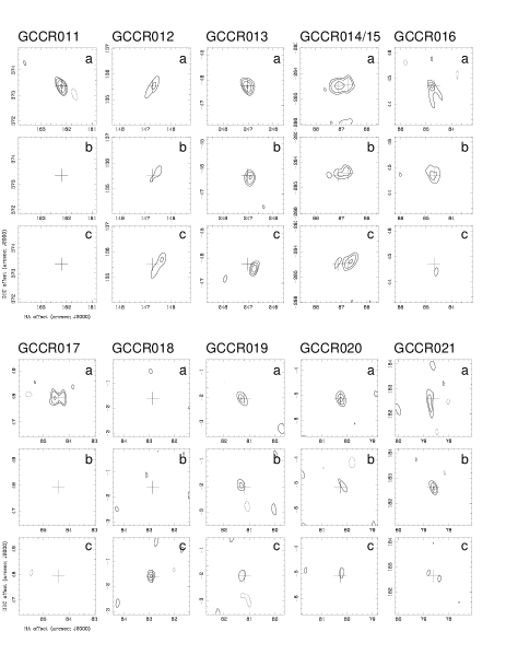
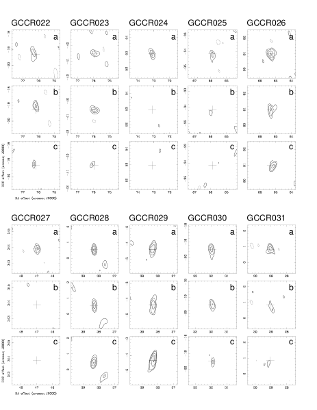
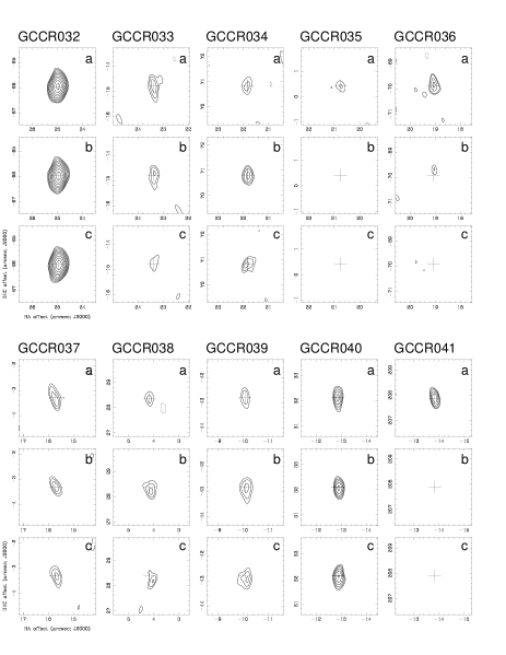
Figure A1: Contour plots for individual GCCR sources at epochs 2019-9-8 (a), 2014-5-26 (b), and 2014-5-17 (c). Each of the sources is arranged in the same column labled with its GCCR ID number at top. Contours are $\sigma_{\rm map}\times$ ($-5$, 5$\times\sqrt{2^{n}}$), where $n=-1$, 0, 1, 2, 3, 4, 5 … until reaching the intensity peak. The rms noises $\sigma_{\rm map}$ are listed in column 11 in Table 2 for corresponding GCCR sources. For the panels of Sgr A*, $\sigma_{\rm map}=10$ mJy beam^-1, a hundred times greater than the local rms noise near the source. The coordinate labels are the angular offsets from the phase center of the date or the pointing center of the VLA observations; the coordinates of the phase center are given in the footnote³ in text.

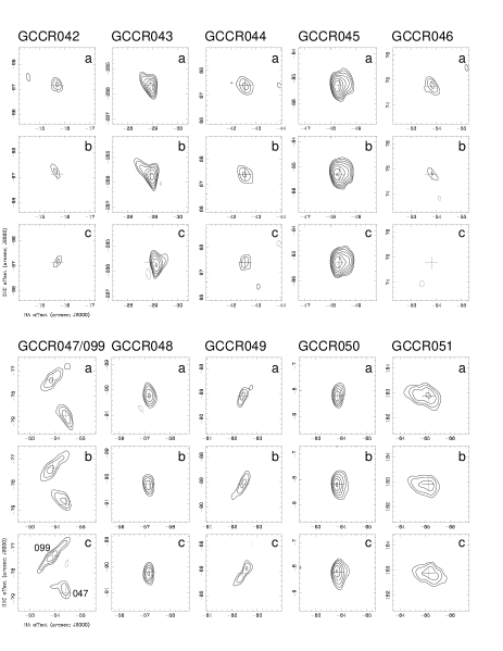
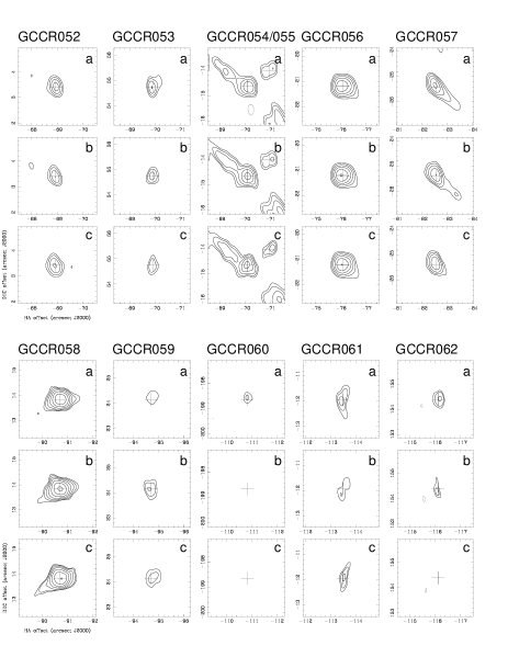
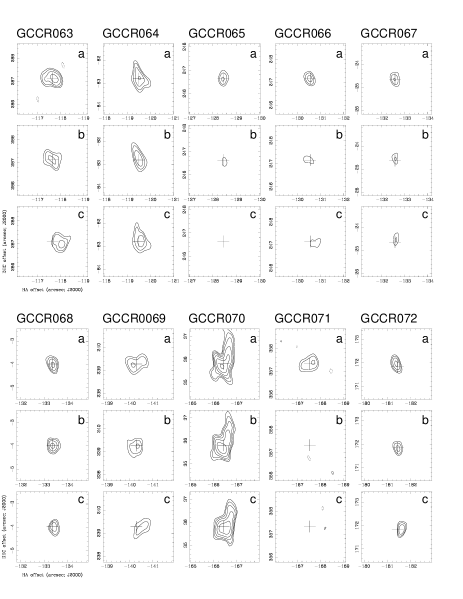
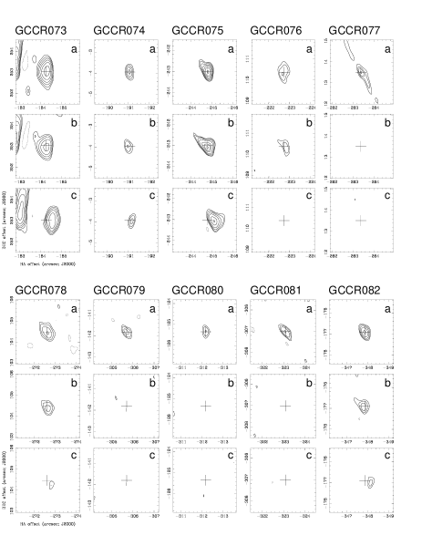
Figure A1: Continued

Figure A1: Continued

Table 2: A catalog of compact radio sources at 5.5 GHz

ID	RA(J2000)    Dec(J2000)	$r_{\theta}$	$\Delta\alpha$	$\Delta\delta$	${\mathscr{F}}_{\rm PB}$	$\sigma{\mathscr{F}}_{\rm PB}^{-1}$	$S\pm\sigma$	$S\pm\sigma$	$S\pm\sigma$	$\sigma_{\rm map}$	Notes
		(arcsec)	(arcsec)				(mJy)	(mJy)	(mJy)	($\mu$Jy bm-1)	r-morph	x-ID
(1)	(2)	(3)	(4)	(5)	(6)	(7)	(8)	(9)	(10)	(11)	(12)	(13)
							2019-09-08	2014-05-26	2014-05-17
Variables and transients -
GCCR001	17:46:10.570 $-$28:55:49.08	453.8	400.6	279.0	42	6.6	17.2$\pm$0.8	7.29$\pm$0.3	$<$4.67	300	u-core	y
GCCR002	17:46:06.132 $-$28:55:56.09	403.7	342.4	272.0	11	1.0	$<0.2$	0.40$\pm$0.03	$<$0.31	35	u-core	n
GCCR003	17:46:01.547 $-$29:01:04.21	251.4	282.1	$-$36.1	2.2	0.03	0.23$\pm$0.02	0.15$\pm$0.02	0.14$\pm$0.02	13	u-core	n
GCCR004	17:45:58.370 $-$28:55:45.28	341.4	240.5	282.8	5.1	0.23	0.87$\pm$0.07	0.68$\pm$0.06	0.58$\pm$0.06	33	u-core	y
GCCR005	17:45:57.717 $-$28:55:13.67	362.4	232.0	314.4	6.5	0.37	0.47$\pm$0.04	0.30$\pm$0.03	0.36$\pm$0.03	33	u-core	n
GCCR006	17:45:58.348 $-$28:53:31.86	455.0	240.3	416.3	45	7.1	12.5$\pm$0.9	2.68$\pm$0.25	1.86$\pm$0.18	300	u-core	n
GCCR007	17:45:57.931 $-$28:59:12.88	209.9	234.7	75.2	1.7	0.017	0.55$\pm$0.03	0.40$\pm$0.02	0.47$\pm$0.02	13	c-core1	n
GCCR008	17:45:57.165 $-$28:58:44.37	211.5	224.7	103.7	1.7	0.018	0.47$\pm$0.03	0.28$\pm$0.02	0.30$\pm$0.02	13	u-core	n
GCCR009	17:45:57.117 $-$28:58:02.35	232.6	224.0	145.8	2.0	0.025	0.42$\pm$0.04	0.34$\pm$0.04	0.25$\pm$0.04	14	c-core2	n
GCCR010	17:45:57.107 $-$28:57:56.17	236.1	223.9	151.9	2.0	0.027	0.46$\pm$0.04	0.41$\pm$0.04	0.32$\pm$0.03	14	c-core3	n
GCCR011	17:45:55.082 $-$28:54:04.61	407.1	197.4	383.5	12	1.1	1.20$\pm$0.11	$<$0.05	$<$0.07	50	u-core	n
GCCR012	17:45:53.901 $-$28:58:02.45	199.8	181.8	145.7	1.6	0.014	0.63$\pm$0.04	0.56$\pm$0.04	0.74$\pm$0.05	34	l-core4	n
GCCR013	17:45:50.764 $-$29:00:39.19	107.8	140.7	$-$11.1	1.1	0.004	0.09$\pm$0.01	0.05$\pm$0.01	0.06$\pm$0.01	13	u-core	n
GCCR014	17:45:49.359 $-$29:04:42.47	278.5	122.2	$-$254.4	2.8	0.061	0.21$\pm$0.01	0.12$\pm$0.01	0.11$\pm$0.01	20	u-core	y
GCCR015	17:45:49.330 $-$29:04:42.41	278.3	121.8	$-$254.3	2.7	0.060	0.19$\pm$0.01	0.15$\pm$0.01	0.16$\pm$0.01	20	u-core	y
GCCR016	17:45:49.174 $-$28:59:33.27	95.8	119.8	54.8	1.1	0.004	0.18$\pm$0.01	0.15$\pm$0.01	0.14$\pm$0.01	7	t-core5	n
GCCR017	17:45:49.153 $-$28:59:30.03	97.1	119.5	58.1	1.1	0.004	0.17$\pm$0.01	$<$0.11	$<$0.10	7	d-core6	n
GCCR018	17:45:49.034 $-$29:00:19.57	82.9	118.0	8.5	1.1	0.004	0.10$\pm$0.02	$<$0.03	0.10$\pm$0.01	9	c-core7	n
GCCR019	17:45:48.908 $-$29:00:19.99	81.2	116.3	8.1	1.1	0.003	0.10$\pm$0.01	0.08$\pm$0.01	0.07$\pm$0.01	7	c-core8	n
GCCR020	17:45:48.837 $-$29:00:23.07	80.5	115.4	5.0	1.1	0.003	0.11$\pm$0.01	0.10$\pm$0.02	0.06$\pm$0.01	7	u-core	n
GCCR021	17:45:48.711 $-$28:57:15.33	198.8	113.8	192.8	1.6	0.014	0.08$\pm$0.02	0.07$\pm$0.02	$<$0.10	7	u-core	n
GCCR022	17:45:48.525 $-$29:00:37.25	78.6	111.3	$-$9.1	1.1	0.003	0.08$\pm$0.01	0.08$\pm$0.01	0.05$\pm$0.01	6	u-core	n
GCCR023	17:45:48.508 $-$29:00:58.51	86.1	111.1	$-$30.4	1.1	0.004	0.08$\pm$0.01	0.10$\pm$0.01	0.04$\pm$0.01	7	u-core	n
GCCR024	17:45:48.291 $-$28:59:25.02	90.2	108.2	63.1	1.1	0.004	0.09$\pm$0.01	$<$0.02	$<$0.03	7	u-core	n
GCCR025	17:45:47.740 $-$29:00:52.12	74.2	101.0	$-$24.0	1.1	0.003	0.23$\pm$0.02	0.16$\pm$0.02	$<$0.05	5	c-core9	n
GCCR026	17:45:47.696 $-$28:58:47.00	112.0	100.4	101.1	1.2	0.004	0.16$\pm$0.01	0.13$\pm$0.02	0.10$\pm$0.01	7	c-core10	n
GCCR027	17:45:46.300 $-$28:54:34.08	347.1	82.1	354.0	5.4	0.26	0.30$\pm$0.03	$<0.07$	$<0.06$	25	u-core	n
GCCR028	17:45:45.638 $-$29:00:17.43	38.3	73.4	10.7	1.0	0.003	0.14$\pm$0.01	0.10$\pm$0.01	0.12$\pm$0.01	10	c-core11	n
GCCR029	17:45:45.638 $-$29:00:22.31	38.5	73.4	5.8	1.0	0.003	0.31$\pm$0.01	0.31$\pm$0.01	0.40$\pm$0.02	12	l-core12	n
GCCR030	17:45:45.151 $-$29:00:37.45	37.4	67.0	$-$9.3	1.0	0.003	0.15$\pm$0.01	0.12$\pm$0.01	0.10$\pm$0.01	9	c-core13	n
GCCR031	17:45:44.932 $-$29:00:17.14	29.0	64.2	11.0	1.0	0.003	0.10$\pm$0.01	0.07$\pm$0.01	0.06$\pm$0.01	6	c-core14	y
GCCR032	17:45:44.622 $-$29:01:23.93	70.5	60.1	$-$55.8	1.1	0.003	2.23$\pm$0.01	2.48$\pm$0.01	2.34$\pm$0.01	13	c-core15	y
GCCR033	17:45:44.500 $-$29:00:32.75	27.7	58.5	$-$4.6	1.0	0.003	0.19$\pm$0.02	0.13$\pm$0.01	0.09$\pm$0.01	7	c-core16	n
GCCR034	17:45:44.382 $-$28:59:07.15	74.1	56.9	81.0	1.1	0.003	0.07$\pm$0.01	0.14$\pm$0.01	0.10$\pm$0.01	7	c-core17	n
GCCR035	17:45:44.300 $-$29:00:17.56	20.8	55.9	10.6	1.0	0.003	0.12$\pm$0.01	$<$0.02	$<$0.02	10	u-core	y
GCCR036	17:45:44.172 $-$29:01:27.87	72.5	54.2	$-$59.8	1.1	0.003	0.20$\pm$0.01	0.11$\pm$0.02	$<0.04$	8	c-core18	y
GCCR037	17:45:43.916 $-$29:00:21.27	16.0	50.8	6.8	1.0	0.003	0.25$\pm$0.02	0.17$\pm$0.02	0.17$\pm$0.02	10	c-core19	y?
GCCR038	17:45:43.036 $-$28:59:49.60	28.7	39.3	38.5	1.0	0.003	0.10$\pm$0.01	0.20$\pm$0.02	0.15$\pm$0.02	10	c-core20	y?
GCCR039	17:45:42.623 $-$29:00:24.80	6.9	34.3	3.3	1.0	0.003	0.17$\pm$0.02	0.22$\pm$0.02	0.30$\pm$0.02	10	c-core21	n
GCCR040	17:45:41.950 $-$29:01:00.78	44.0	25.0	$-$32.7	1.0	0.003	0.20$\pm$0.02	0.38$\pm$0.02	0.35$\pm$0.02	13	c-core22	n
GCCR041	17:45:41.664 $-$28:56:50.09	208.3	21.3	218.0	1.7	0.017	0.22$\pm$0.02	$<$0.03	$<$0.03	10	c-core23	y?
GCCR042	17:45:41.522 $-$29:01:54.82	98.1	19.4	$-$86.7	1.1	0.004	0.13$\pm$0.01	0.09$\pm$0.01	0.08$\pm$0.01	10	u-core	n
GCCR043	17:45:40.515 $-$29:05:03.65	287.1	6.2	$-$275.5	3.0	0.072	1.04$\pm$0.03	1.05$\pm$0.03	0.90$\pm$0.03	24	c-core24	n
GCCR044	17:45:39.474 $-$28:59:10.58	79.7	$-$7.4	77.5	1.1	0.003	0.49$\pm$0.02	0.50$\pm$0.02	0.38$\pm$0.02	18	c-core25	n
GCCR045	17:45:39.034 $-$29:01:43.24	98.0	$-$13.2	$-$75.1	1.1	0.004	1.00$\pm$0.02	1.19$\pm$0.02	1.21$\pm$0.02	11	t-core26	n
GCCR046	17:45:38.617 $-$28:59:03.21	92.1	$-$18.7	84.9	1.1	0.004	0.30$\pm$0.02	0.16$\pm$0.02	$<$0.05	13	c-core27	n
GCCR047	17:45:38.571 $-$29:01:36.75	95.7	$-$19.3	$-$68.6	1.1	0.004	0.32$\pm$0.02	0.34$\pm$0.02	0.29$\pm$0.01	13	c-core28	y
GCCR048	17:45:38.358 $-$29:01:48.19	106.8	$-$22.1	$-$80.1	1.1	0.004	0.26$\pm$0.01	0.19$\pm$0.01	0.21$\pm$0.01	9	c-core29	n
GCCR049	17:45:37.958 $-$29:01:47.05	108.8	$-$27.3	$-$78.9	1.1	0.004	0.28$\pm$0.02	0.37$\pm$0.03	0.28$\pm$0.02	13	c-core30	y
GCCR050	17:45:37.850 $-$29:00:26.15	64.4	$-$28.7	2.0	1.0	0.003	0.66$\pm$0.01	0.97$\pm$0.02	0.94$\pm$0.02	22	c-core31	y
GCCR051	17:45:37.753 $-$28:57:15.07	194.2	$-$30.0	193.0	1.6	0.013	1.23$\pm$0.05	0.92$\pm$0.04	1.15$\pm$0.04	23	l-core32	n
GCCR052	17:45:37.463 $-$29:00:14.55	69.1	$-$33.8	13.6	1.1	0.003	0.89$\pm$0.02	0.71$\pm$0.02	0.97$\pm$0.02	29	c-core33	n
GCCR053	17:45:37.390 $-$28:59:23.23	88.8	$-$34.8	64.9	1.1	0.004	0.29$\pm$0.02	0.22$\pm$0.02	0.18$\pm$0.01	12	t-core34	n
GCCR054	17:45:37.375 $-$29:00:32.61	71.5	$-$35.0	$-$4.5	1.1	0.003	1.54$\pm$0.02	1.95$\pm$0.02	1.82$\pm$0.02	35	l-core35	n
GCCR055	17:45:37.310 $-$29:00:31.98	72.3	$-$35.8	$-$3.9	1.1	0.003	0.84$\pm$0.02	0.78$\pm$0.02	0.56$\pm$0.01	35	d-core36	n
GCCR056	17:45:36.920 $-$29:00:39.17	78.9	$-$40.9	$-$11.1	1.1	0.003	8.16$\pm$0.03	8.08$\pm$0.03	8.40$\pm$0.03	110	t-core37	y
GCCR057	17:45:36.425 $-$29:00:43.37	86.3	$-$47.4	$-$15.3	1.1	0.004	0.66$\pm$0.02	0.62$\pm$0.02	0.54$\pm$0.02	13	t-core38	y
GCCR058	17:45:35.804 $-$29:00:04.13	91.6	$-$55.6	24.0	1.1	0.003	1.28$\pm$0.02	1.49$\pm$0.02	1.49$\pm$0.02	14	l-core39	y
GCCR059	17:45:35.499 $-$28:59:53.83	97.7	$-$59.6	34.3	1.1	0.004	0.17$\pm$0.02	0.23$\pm$0.02	0.25$\pm$0.02	11	c-core40	y?
GCCR060	17:45:34.271 $-$29:03:36.62	227.4	$-$75.7	$-$188.5	1.9	0.023	0.13$\pm$0.01	$<$0.08	$<$0.09	10	c-core41	n
GCCR061	17:45:34.068 $-$29:00:29.91	114.0	$-$78.4	$-$1.8	1.2	0.004	0.24$\pm$0.02	0.15$\pm$0.02	0.19$\pm$0.02	9	l-core42	y
GCCR062	17:45:33.867 $-$28:57:43.58	193.1	$-$81.0	164.5	1.6	0.013	0.24$\pm$0.02	0.12$\pm$0.02	$<$0.05	9	c-core43	n
GCCR063	17:45:33.749 $-$28:55:30.85	310.3	$-$82.6	297.3	3.7	0.11	0.82$\pm$0.02	0.60$\pm$0.02	0.58$\pm$0.02	20	l-core44	n

Table 2: $-$ Continued

ID	RA(J2000)    Dec(J2000)	$r_{\theta}$	$\Delta\alpha$	$\Delta\delta$	${\mathscr{F}}_{\rm PB}$	$\sigma{\mathscr{F}}_{\rm PB}^{-1}$	$S\pm\sigma$	$S\pm\sigma$	$S\pm\sigma$	$\sigma_{\rm map}$	Notes
		(arcsec)	(arcsec)				(mJy)	(mJy)	(mJy)	($\mu$Jy bm-1)	r-morph	x-ID
(1)	(2)	(3)	(4)	(5)	(6)	(7)	(8)	(9)	(10)	(11)	(12)	(13)
							2019-09-08	2014-05-26	2014-05-17
GCCR064	17:45:33.610 $-$29:01:40.76	145.4	$-$84.4	$-$72.6	1.3	0.006	0.66$\pm$0.02	0.55$\pm$0.02	0.60$\pm$0.02	16	t-core45	y
GCCR065	17:45:32.927 $-$28:56:11.34	278.1	$-$ 93.4	256.8	2.7	0.060	0.26$\pm$0.02	0.14$\pm$0.02	$<$0.10	19	c-core46	n
GCCR066	17:45:32.767 $-$28:56:10.82	279.5	$-$ 95.5	257.3	2.8	0.062	0.35$\pm$0.02	0.25$\pm$0.02	0.20$\pm$0.02	22	u-core	n
GCCR067	17:45:32.613 $-$29:00:42.60	134.9	$-$ 97.4	$-$14.5	1.2	0.006	0.15$\pm$0.01	0.08$\pm$0.01	0.08$\pm$0.01	10	c-core47	y
GCCR068	17:45:32.552 $-$29:00:21.95	133.4	$-$ 98.3	6.2	1.2	0.005	0.18$\pm$0.01	0.19$\pm$0.01	0.14$\pm$0.01	9	u-core	n
GCCR069	17:45:32.025 $-$28:56:18.70	277.4	$-$105.2	249.4	2.7	0.059	0.82$\pm$0.03	0.70$\pm$0.03	0.60$\pm$0.03	24	l-core48	n
GCCR070	17:45:30.031 $-$28:59:42.17	170.3	$-$131.3	45.9	1.4	0.009	1.28$\pm$0.03	1.11$\pm$0.03	1.12$\pm$0.03	12	t-core49	y
GCCR071	17:45:29.947 $-$28:54:20.64	394.7	$-$132.5	367.5	10	0.83	1.39$\pm$0.12	$<0.16$	$<0.20$	48	t-core50	n
GCCR072	17:45:28.892 $-$28:57:26.02	249.9	$-$146.3	182.1	2.2	0.035	0.23$\pm$0.02	0.15$\pm$0.01	0.17$\pm$0.01	13	u-core	y
GCCR073	17:45:28.671 $-$28:56:04.94	313.0	$-$149.2	263.2	3.8	0.12	8.78$\pm$0.03	5.85$\pm$0.03	7.12$\pm$0.03	100	c-core51	y
GCCR074	17:45:28.154 $-$29:00:21.91	190.9	$-$155.9	6.2	1.6	0.012	0.18$\pm$0.01	0.13$\pm$0.01	0.12$\pm$0.01	10	u-core	y?
GCCR075	17:45:24.057 $-$29:04:20.98	344.8	$-$209.6	$-$232.9	5.3	0.24	1.80$\pm$0.05	2.20$\pm$0.09	1.76$\pm$0.09	40	u-core	n
GCCR076	17:45:25.740 $-$28:58:27.60	248.5	$-$187.6	120.5	2.2	0.034	0.36$\pm$0.03	0.25$\pm$0.02	0.22$\pm$0.02	13	t-core52	n
GCCR077	17:45:22.641 $-$29:00:04.46	263.7	$-$228.3	23.7	2.5	0.045	0.20$\pm$0.02	$<$0.06	$<$0.06	15	l-core53	y?
GCCR078	17:45:21.937 $-$28:58:33.50	292.0	$-$237.5	114.6	3.1	0.079	0.44$\pm$0.02	0.27$\pm$0.02	0.16$\pm$0.01	14	c-core54	n
GCCR079	17:45:19.415 $-$29:02:39.78	337.0	$-$270.5	$-$131.7	4.8	0.20	0.25$\pm$0.02	$<$0.08	$<$0.1	20	u-core	n
GCCR080	17:45:18.921 $-$29:02:23.32	336.4	$-$277.0	$-$115.2	4.8	0.20	0.21$\pm$0.02	$<$0.07	$<$0.08	20	u-core	n
GCCR081	17:45:18.090 $-$29:05:24.99	445.6	$-$287.9	$-$296.9	30	4.3	1.93$\pm$0.19	0.80$\pm$0.19	$<$0.06	120	u-core	n
GCCR082	17:45:16.201 $-$29:03:14.87	390.1	$-$312.7	$-$166.8	9.5	0.74	1.22$\pm$0.05	0.98$\pm$0.05	0.61$\pm$0.06	50	u-core	y
							2019-09-08	2014-05-26	2014-05-17
Non-variables -
GCCR083	17:45:54.472 $-$29:02:27.17	201.2	189.3	$-$119.1	1.6	0.015	0.16$\pm 0$.01	0.17$\pm$0.01	0.16$\pm$0.01	10	u-core	n
GCCR084	17:45:51.214 $-$29:00:00.91	112.9	146.6	27.2	1.2	0.004	0.10$\pm$0.01	0.11$\pm$0.01	0.10$\pm 0.01$	10	u-core	n
GCCR085	17:45:50.620 $-$28:59:19.45	119.0	138.8	68.7	1.2	0.005	0.10$\pm 0.01$	0.11$\pm$0.01	0.09$\pm$0.01	7	u-core	y
GCCR086	17:45:48.794 $-$29:01:36.89	112.2	114.8	$-$68.8	1.2	0.004	0.12$\pm$0.01	0.14$\pm$0.01	0.12$\pm$0.01	10	u-core	n
GCCR087	17:45:48.676 $-$29:03:51.03	226.9	113.2	$-$202.9	1.9	0.023	0.15$\pm$0.01	0.14$\pm$0.01	0.14$\pm$0.01	11	u-core	y
GCCR088	17:45:47.834 $-$29:00:01.23	69.2	102.2	26.9	1.1	0.003	0.22$\pm$0.02	0.24$\pm$0.02	0.25$\pm$0.02	10	l-core55	n
GCCR089	17:45:45.522 $-$28:58:28.39	115.6	71.9	119.7	1.2	0.005	0.54$\pm$0.02	0.55$\pm$0.02	0.53$\pm$0.02	9	l-core56	y
GCCR090	17:45:45.109 $-$28:58:44.54	98.5	66.5	103.6	1.1	0.004	0.20$\pm$0.01	0.21$\pm$0.01	0.21$\pm$0.01	9	c-core57	n
GCCR091	17:45:45.060 $-$29:02:32.57	138.1	65.8	$-$124.5	1.3	0.006	0.47$\pm$0.02	0.44$\pm$0.02	0.45$\pm$0.02	10	c-core58	n
GCCR092	17:45:44.805 $-$29:00:19.72	27.6	62.5	8.4	1.0	0.003	0.09$\pm$0.01	0.10$\pm$0.01	0.10$\pm$0.01	8	c-core59	y?
GCCR093	17:45:43.926 $-$28:59:36.02	44.8	51.0	52.1	1.0	0.003	0.24$\pm$0.02	0.20$\pm$0.02	0.19$\pm$0.02	10	t-core60	n
GCCR094	17:45:43.094 $-$29:01:48.66	90.8	40.0	$-$80.5	1.1	0.004	0.21$\pm$0.02	0.20$\pm$0.02	0.22$\pm$0.02	10	c-core61	n
GCCR095	17:45:42.869 $-$28:59:54.39	23.7	37.1	33.7	1.0	0.003	0.55$\pm$0.02	0.55$\pm$0.02	0.55$\pm$0.02	20	l-core62	y?
GCCR096	17:45:42.570 $-$29:00:34.19	16.3	33.2	$-$6.1	1.0	0.003	0.29$\pm$0.02	0.27$\pm$0.02	0.27$\pm$0.02	10	l-core63	y?
GCCR097	17:45:42.346 $-$29:00:23.03	7.0	30.2	5.1	1.0	0.003	2.24$\pm$0.07	2.41$\pm$0.07	2.44$\pm$0.07	20	t-core64	y?
GCCR098	17:45:41.737 $-$28:59:45.85	34.6	22.2	42.3	1.0	0.003	0.28$\pm$0.02	0.33$\pm$0.02	0.28$\pm$0.02	10	c-core65	y
GCCR099	17:45:38.610 $-$29:01:35.31	94.3	$-$18.8	$-$67.2	1.1	0.004	0.40$\pm$0.04	0.40$\pm$0.04	0.43$\pm$0.04	13	l-core66	y?
GCCR100	17:45:38.586 $-$28:59:32.21	70.9	$-$19.1	55.9	1.1	0.003	0.23$\pm$0.01	0.24$\pm$0.01	0.23$\pm$0.01	12	c-core67	y?
GCCR101	17:45:37.756 $-$29:00:34.02	67.1	$-$30.0	$-$5.9	1.1	0.003	0.39$\pm$0.02	0.44$\pm$0.02	0.39$\pm$0.02	12	t-core68	y?
GCCR102	17:45:36.888 $-$29:00:25.49	76.8	$-$41.4	2.6	1.1	0.003	0.24$\pm$0.02	0.23$\pm$0.02	0.26$\pm$0.02	11	c-core69	n
GCCR103	17:45:36.858 $-$29:01:17.46	97.2	$-$41.8	$-$49.3	1.1	0.004	0.24$\pm$0.02	0.22$\pm$0.01	0.22$\pm$0.01	10	u-core	y?
GCCR104	17:45:36.818 $-$29:00:29.54	78.2	$-$42.3	$-$1.4	1.1	0.003	0.40$\pm$0.02	0.41$\pm$0.02	0.40$\pm$0.02	16	c-core70	n
GCCR105	17:45:36.613 $-$28:59:56.60	82.9	$-$45.0	31.5	1.1	0.004	0.30$\pm$0.02	0.34$\pm$0.02	0.32$\pm$0.02	20	c-core71	n
GCCR106	17:45:36.274 $-$29:00:42.63	88.0	$-$49.4	$-$14.5	1.1	0.004	0.22$\pm$0.02	0.23$\pm$0.02	0.22$\pm$0.02	9	c-core72	y?
GCCR107	17:45:36.149 $-$28:56:38.24	236.0	$-$51.1	229.9	2.0	0.027	0.09$\pm$0.01	0.12$\pm$0.01	0.10$\pm$0.01	9	u-core	y
GCCR108	17:45:35.730 $-$28:58:42.00	132.8	$-$56.6	106.1	1.2	0.005	1.51$\pm$0.04	1.58$\pm$0.04	1.58$\pm$0.04	10	l-core73	n
GCCR109	17:45:35.553 $-$29:00:47.11	98.4	$-$58.9	$-$19.0	1.1	0.004	0.23$\pm$0.03	0.27$\pm$0.03	0.23$\pm$0.03	10	l-core74	n
GCCR110	17:45:32.758 $-$28:56:16.37	274.6	$-$95.4	251.8	2.7	0.056	0.23$\pm$0.02	0.21$\pm$0.02	0.23$\pm$0.03	11	u-core	y

Table 2: $-$ Continued

Note to Table 2 $-$ Listed below are the source sizes $\theta_{\rm maj}\pm\sigma,\theta_{\rm min}\pm\sigma$, PA${}_{\Theta}\pm\sigma$ in the units of (arcsec,arcsec, deg):
10.20$\pm 0.02,0.12\pm 0.01$, 17$\pm$5;	20.63$\pm 0.10,0.29\pm 0.10$, 34$\pm$11;	30.67$\pm 0.12,0.31\pm 0.11$, 18$\pm$10;	40.96$\pm 0.05,0.10\pm 0.09$, 148$\pm$5;
50.75$\pm 0.20,0.31\pm 0.08$, 10$\pm$13;	60.71$\pm 0.10,0.24\pm 0.16$, 108$\pm$12;	70.50$\pm 0.20,0.30\pm$0.17, 50$\pm$30;	80.57$\pm 0.12,0.1\pm 0.1$, 71$\pm$15;
90.65$\pm 0.10,0.28\pm$0.10, 130$\pm$10;	100.46$\pm 0.1,0.20\pm 0.08$, 85$\pm$21;	110.32$\pm 0.05,0.04\pm$0.03, 15$\pm$4;	120.80$\pm 0.10,0.21\pm$0.04, 164$\pm$3;
130.50$\pm 0.10,0.17\pm$0.08, 20$\pm$13;	140.35$\pm 0.13,0.26\pm$0.12, 68$\pm$21;	150.37$\pm 0.03,0.28\pm$0.03, 160$\pm$3;	160.51$\pm 0.07,0.24\pm$0.03, $-4\pm$4;
170.28$\pm 0.04,0.23\pm$0.02, 22$\pm$5;	180.61$\pm 0.16,0.28\pm$0.06, 13$\pm$8;	190.77$\pm 0.08,0.26\pm$0.07, 20$\pm$6;	200.50$\pm 0.10,0.33\pm$0.06, 174$\pm$25;
210.40$\pm 0.08,0.22\pm$0.07, 35$\pm$7;	220.55$\pm 0.10,0.25\pm$0.05, 4$\pm$8;	230.41$\pm 0.12,0.11\pm$0.06, 22$\pm$10;	240.47$\pm 0.08,0.14\pm 0.05$, 41$\pm$8;
250.68$\pm 0.09,0.43\pm$0.07, 67$\pm$15;	260.40$\pm 0.03,0.37\pm$0.03, 146$\pm$19;	270.53$\pm 0.21,0.14\pm$0.20, 57$\pm$23;	280.65$\pm 0.07,0.12\pm$0.08, 41$\pm$5;
290.35$\pm 0.07,0.16\pm$0.04, 20$\pm$10;	300.98$\pm 0.05,0.05\pm$0.05, 144$\pm$6;	310.39$\pm 0.05,0.21\pm$0.02, 5$\pm$15;	320.74$\pm 0.10,0.45\pm$0.05, 64$\pm$6;
330.55$\pm 0.05,0.41\pm$0.03, 49$\pm$8;	340.46$\pm 0.07,0.33\pm$0.04, 170$\pm$15;	350.55$\pm 0.05,0.38\pm$0.03, 80$\pm$5;	360.59$\pm 0.04,0.34\pm$0.03, 124$\pm$5;
370.62$\pm 0.04,0.42\pm$0.03, 78$\pm$15, a core of M source (Yusef-Zadeh & Morris, 1987; Zhao, Morris & Goss, 2013);
380.63$\pm 0.03,0.31\pm$0.04, 43$\pm$5;	390.62$\pm 0.04,0.31\pm$0.03, 90$\pm$4;	400.61$\pm 0.10,0.43\pm$0.10, 138$\pm$16;	410.50$\pm 0.20,0.20\pm$0.15, 134$\pm$30;
420.90$\pm 0.10,0.25\pm$0.05, 176$\pm$4;	430.70$\pm 0.10,0.37\pm$0.10, 32$\pm$12;	440.54$\pm 0.05,0.37\pm$0.07, 97$\pm$10;	450.76$\pm 0.11,0.46\pm$0.07, 35$\pm$10;
460.28$\pm 0.05,0.14\pm$0.13, 63$\pm$20;	470.39$\pm 0.10,0.23\pm$0.10, 40$\pm$25;	480.70$\pm 0.05,0.36\pm$0.05, 88$\pm$5;	490.83$\pm 0.05,0.51\pm$0.03, 154$\pm$5;
500.65$\pm 0.15,0.10\pm$0.10, 99$\pm$20;	510.72$\pm 0.05,0.35\pm$0.05, 5$\pm$3, source H2 (Yusef-Zadeh & Morris, 1987; Zhao et al., 1993);
520.69$\pm 0.25,0.30\pm$0.07, 20$\pm$10;	530.77$\pm 0.21,0.38\pm$0.11, 29$\pm$21;	540.43$\pm 0.07,0.28\pm$0.07, 67$\pm$19;	550.91$\pm 0.10,0.20\pm 0.05$, 172$\pm$5;
560.85$\pm 0.06,0.31\pm 0.05$, 84$\pm$5, the core of Cannonball(Zhao, Morris & Goss, 2013);
570.43$\pm 0.06,0.12\pm$0.03, 42$\pm$7;	580.49$\pm 0.10,0.45\pm$0.13, 60$\pm$20;	590.36$\pm 0.13,0.18\pm$0.08, 132$\pm$20;	600.63$\pm 0.17,0.32\pm$0.07, 150$\pm$15;
610.63$\pm 0.12,0.23\pm$0.06, 45$\pm$10;	620.75$\pm 0.10,0.36\pm$0.07, 15$\pm$5;	630.60$\pm 0.05,0.20\pm$0.05, 12$\pm$4;	640.81$\pm 0.03,0.44\pm$0.03, 133$\pm$3;
650.42$\pm 0.03,0.11\pm$0.03, 4$\pm$3;	66one of the pair GCCR047/099;	670.27$\pm 0.05,0.15\pm$0.03, 47$\pm$6;	680.44$\pm 0.05,0.29\pm$0.07, 122$\pm$12;
690.43$\pm 0.09,0.18\pm$0.04, 17$\pm$6;	700.60$\pm 0.10,0.47\pm$0.06, 33$\pm$14;	710.24$\pm 0.04,0.14\pm$0.07, 136$\pm$22;	720.30$\pm 0.06,0.29\pm$0.08, 98$\pm$30;
730.80$\pm$0.06,0.45$\pm$0.04,50$\pm$10;	740.54$\pm 0.10\times 0.12\pm$0.10, 67$\pm$20;

References

- Abramowicz & Fragile (2013) Abramowicz, M. A. & Fragile, P. C. 2013, LRR, 16, 1
- Aharon & Perets (2015) Aharon, D. & Perets, H. B. 2015, ApJ, 799, 185
- Aizu (1973) Aizu, K. 1973, PThPh, 50, 344
- Antonini et al. (2015) Antonini, F., Barausse, E., Silk, J. 2015, ApJ, 812, 72
- Arca-Sedda & Capuzzo-Dolcetta (2017) Arca-Sedda, M. & Capuzzo-Dolcetta, R. 2017, MNRAS, 471, 478
- Barrett et al. (2017) Barrett, P. E., Dieck, C., Beasley, A. J., et al. 2017, AJ, 154, 252
- Barrett et al. (2020) Barrett, P. E., Dieck, C., Beasley, A. J., et al. 2020, invited talk for COSPAR 42nd General Assembly, Pasadena, CA, arXiv:2004.11418v2
- Bates et al. (2011) Bates, S. D., Johnston, S., Lorimer, D. R., et al. 2011, MNRAS, 411, 1575
- Bird et al. (2016) Bird, A. J., Bazzano, A., Malizia, A., et al. 2016, ApJS, 223, 15
- Blandford et al. (2019) Blandford, R. Meier, D., & Readhead, A. 2019, ARA&A, 57, 467
- Blandford & Begelman (1999) Blandford, R. D. & Begelman M. C. 1999, MNRAS, 303, L1
- Bower et al. (2018) Bower, G. C., Chatterjee, S. Cordes, J. et al. 2018, Science with a Next Generation Very Large Array, ASP Monograph 7. edited by Eric Murphy, ASP Conf. Series, Vol. 517, 793
- Bower et al. (2014) Bower, G. C., Deller, A., Demorest, P. et al. 2014, ApJ, 780, L2
- Bridle & Schwab (1999) Bridle, A. H. & Schwab, F. R. 1999, Synthesis Imaging in Radio Astronomy II, A Collection of Lectures from the Sixth NRAO/NMIMT Synthesis Imaging Summer School, Edited by G. B. Taylor, C. L. Carilli, and R. A. Perley. ASP Conference Series, Vol. 180, 371
- Brook, et al. (2018) Brook, P. R., Karastergiou, A., McLaughlin, M. A., et al. 2018, ApJ, 868, 122.
- Clark et al. (2009) Clark, J. S., Crowther, P. A., Mikles, V. J. 2009, AA, 507, 1567
- Condon et al. (2012) Condon, J. J., Cotton, W. D., Fomalont, E. B., et al. 2012, ApJ, 758, 23
- Corbel et al. (2000) Corbel, S., Fender, R. P., Tzioumis, A. K. et al. 2000, AA, 359, 251
- Corbel et al. (2003) Corbel, S., Nowak, M. A., Fender, R. P., et al. 2003, AA, 400, 1007
- Corbel et al. (2008) Corbel, S., Kr̈ding, E. Kaaret, P. 2008, MNRAS, 389, 1697
- Cordes & Lazio (1997) Cordes, J. M. & Lazio, T. J. W. 1997, ApJ, 475, 557
- Coriat et al. (2011) Coriat, M., Corbel, S., Prat, L. et al. 2011, MNRAS, 414, 677
- Copperjans & Knigge (2020) Coppejans, D. & Knigge, C. 2020, to appear in New Astronomy Reviews special volume ’100 Years of Astrophysical Jets’ (eds. Rob Fender and Ralph Wijers), arXiv:2003.05953
- Degenaar & Wijnands (2010) Degenaar, N. & Wijnands, R. 2010, A&A, 524, A69
- Degenaar et al. (2015) Degenaar, N., Wiljnands, R., Miller, J. M., et al. 2015, JHE Astroph., 7, 137
- DeWitt et al. (2013) DeWitt, C. Bandyopadhyay, R. M., Eikenberry, S. S., et al. 2013, AJ, 146, 109
- Dexter & O’Leary (2014) Dexter, J. & O’Leary, R. M. 2014, ApJL, 783, L7
- Eatough et al. (2015) Eatough, R. P., Lazio, T. J. W. Casanellas, J., et al. 2015, Observing Radio Pulsars in the Galactic Centre with the Square Kilometre Array, “Advancing Astrophysics with the Square Kilometre Array”, Proceedings of Science, PoS(AASKA14)045
- Eatough et al. (2013a) Eatough, R. P., Falcke, H., Karuppusamy, R., et al. 2013a, Nature, 501, 391.
- Eatough et al. (2013b) Eatough, R. P., Kramer, M., Klein, B., et al. 2013b, in Neutron Stars and Pulsars: Challenges and Opportunities after 80 years, (Cambridge University Press, Cambridge), Proc. of IAUS 291, 382
- Ekers et al. (1983) Ekers, R. D., Goss, W. M., Schwarz, U. J.,Downes, D., & Rogstad, D. H. 1983, AA, 122, 143
- Feldmeier et al. (2014) Feldmeier, A., Neumayer, N., Seth, A., et al. 2014, A&A, 570, A2
- Fender et al. (1999) Fender, R., Corbel, S., Tzioumis, T. et al. 1999, ApJL, 519, L165
- Fender et al. (2009) Fender, R., Homan, J., Belloni, T. M. 2009, MNRAS, 396, 1370
- Gallo et al. (2003) Gallo, E., Fender, R. P. & Pooley, G. G. 2003, MNRAS, 344, 60
- Gallo et al. (2018) Gallo, E., Degenaar, N., van den Eijinden, J. 2018, MNRAS, 478, L117
- Genzel et al. (2010) Genzel, R., Eisenhauer, F. & Gillessen, S. 2010, Rev. of Mod. Phys., 82, 3121
- Ghez et al. (2005) Ghez, A. M., Salim, S., Hornstein, S. D., et al. 2005, ApJ, 620, 744
- Gim et al. (2019) Gim, H. B., Yun, M. S., Owen, F. N., et al. 2019, ApJ, 875, 80
- Goss et al. (1985) Goss, W. M., Schwarz, U. J., van Gorkom, J. H., & Ekers, R. D. 1985, MNRAS, 215, 69
- Haggard et al. (2017) Haggard, D., Heinke, C. Hooper, D. & Linden, T. 2017, J. Cosmo. Astropart. Phys., 5, 56
- Hailey et al. (2018) Hailey, C. J., Mori, K., Bauer, F. E., et al. 2018, Nature 256, 70
- Hailey et al. (2016) Hailey, C. J., Mori, K., Perez, Kerstin, et al 2016, ApJ, 826, 160
- Heard & Warwick (2013) Heard, V. & Warwick, R. S. 2013, MNRAS, 428, 346
- Hong et al. (2016) Hong, J., Mori, K., Hailey, C. J., et al. 2016, ApJ, 825, 132
- Johnston et al. (2006) Johnston, S., Kramer, M., Lorimer, D. R., et al. 2006, MNRAS, 373, L6
- Johnston & Kerr (2018) Johnston, S. & Kerr, M. 2018, 474, 4629
- Kennea et al. (2013) Kennea, J. A., Burrows, D. N., Kouveliotou, C., et al. 2013, ApJL, 770, L24
- Kramer et al. (1998) Kramer, M., Xilouris, K. M., Lorimer, D. R., et al. 1998, ApJ, 501, 270
- Kramer et al. (1999) Kramer, M., Lange, C., Lorimer, D. R., et al. 1999, ApJ, 526, 957
- Kramer et al. (2000) Kramer, M., Klein, B., Lorimer, D., Müller, P., Jessner, A., Wielebinski, R. 2000, The Effelsberg Search for Pulsars in the Galactic Centre in Pulsar Astronomy - 2000 and Beyound, edited by M. Kramer, N. Wex, and N. Wielebinski, (San Francisco: ASP), ASP Conf. Series 202, 37
- Kramer et al. (2006) Kramer, M., Lyne, A. G., O’Brien, J. T., Jordan, C. A., Lorimer, D. R. 2006, Science, 312, 549
- Kylafis et al. (2012) Kylafis, N. D., Contopoulos, I., Kazanas, D. & Christodoulou, D. M. 2012, AA, 538, A5
- Ledlow et al. (1992) Ledlow, M. J., Zeilik, M., Burns, J. O., Gisler, G. R., Zhao, J.-H. & Baker, D. N. 1992, ApJ, 384, 640
- Lorimer et al. (1995) Lorimer, D. R., Yates, J. A., Lyne, A. G., & Gould, D. M. 1995, MNRAS, 273, 411
- Lu et al. (2013) Lu, J. R., Do, T., Ghez, A. M., et al. 2013, ApJ, 764, 155
- Macquart & Kanekar (2015) Macquart, J.-P., Kanekar, N. 2015, ApJ, 805, 172
- Macquart et al. (2010) Macquart, J.-P., Kanekar, N.;, Frail, D. A., Ransom, S. M. 2010, ApJ, 715, 939
- Manchester et al. (2005) Manchester, R. N., Hobbs, G. B., Teoh, A. and Hobbs, M. 2005, AJ, 129, 1993
- Mauerhan et al. (2010) Mauerhan, J. C., Muno, M. P., Morris, M. R., Stolovy, S. R., Cotera, A. 2010, ApJ, 710, 706
- Migliari & Fender (2006) Migliari, S.& Fender, R. P. 2006, MNRAS, 366, 79
- Mikles et al. (2008) Mikles, V. J., Eikenberry, S. S., Bandyopadhyay, R. M., Muno, M. P. 2008, ApJ, 689, 1222
- Mills et al. (2011) Mills, E., Morris, M. R., Lang, C. C., Dong, H., Wang, Q. D., Cotera, A., & Stolovy, S. R. 2011, ApJ, 735, 84
- Milosavljević (2004) Milosavljević M. 2004, ApJ, 605, L13
- Mori et al. (2013) Mori, K., Gotthelf, E. V., Zhang, S. et al. 2013, ApJL, 770, L23
- Morris et al. (2017) Morris, R. M., Zhao, Jun-Hui & Goss, W. M. 2017, ApJL, 850, L23
- Muno et al. (2003) Muno, M. P., Baganoff, F. K., Bautz, M. W., et al. 2003, ApJ, 589, 225
- Muno et al. (2004) Muno, M. P., Baganoff, F. K., Bautz, M. W., et al. 2004, ApJ, 613, 326
- Muno et al. (2005) Muno, M. P., Lu, J. R., Baganoff, F. K., et al. 2005, ApJ, 633, 228;
- Muno et al. (2006) Muno, M. P., Bauer, F. E., Bandyopadhyay, R. M., Wang, Q. D. 2006, ApJS, 165, 173
- Muno et al. (2008) Muno, M. P., Baganoff, F. K., Brandt, W. N., et al. 2008, ApJ, 673, 251
- Muno et al. (2009) Muno, M. P., Bauer, F. E., Baganoff, F. K., et al. 2009, ApJS, 181, 110;
- Narayan & Yi (1994) Narayan, R. & Yi, I. 1994, ApJL, 428, L13
- Narayan et al. (1997) Narayan, R., Garcia, M. R. & McClintock, J. E. 1997, ApJ, 452, 710
- Oh et al. (2018) Oh, K., Koss, M., Markwardt, C. B., et al. 2018, ApJS, 235, 4
- Park et al. (2005) Park, S., Muno, M. P., Baganoff, F. K., et al. 2005, ApJ, 631, 964
- Perez et al. (2015) Perez, K., Hailey, C. J., Bauer, F. E., et al. 2015, Nature, 520, 646
- Perley (2016) Perley, R. 2016, NRAO EVLA Memo 195;
- Perley & Butler (2017) Perley, R. A. & Bulter, B. J. 2017, ApJS, 230, 7
- Pfahl & Loeb (2004) Pfahl & Loeb 2004, ApJ, 615, 253
- Qiao & Liu (2019) Qiao, Erlin & Liu, B. F. 2019, MNRAS, 487, 1626
- Rajwade et al. (2017) Rajwade, K. M. Lorimer, D. R., Anderson, L. D. 2017, MNRAS, 471, 730
- Rau & Cornwell (2011) Rau, U. & Cornwell, T. J. 2011, AA, 532, A71
- Remillard & McClintock (2006) Remillard & McClintock 2006, ARAA, 44, 49;
- Schödel (2003) Schödel, R., Ott, T., Genzel, R., et al. (2003, ApJ, 596, 1015
- Schödel (2014) Schödel, R., Feldmeier, A., Kunneriath, D., et al. 2014, A&A, 566, A47
- Schödel (2019) Schödel, R. 2020, in GCWS2019, eds. Masato Tsuboi and Tomoharu Oka.
- Shakura & Sunyaev (1973) Shakura, N. I. & Sunyaev, R. A. 1973, AA, 24, 337
- Spitler et al. (2014) Spitler, L. G., Lee, K. J., Eatough, R. P., et al. 2014, ApJ, 780, L3
- Taylor et al. (1993) Taylor, J. H., Manchester, R., & Lyne, A. G. 1993, ApJS, 88, 529
- Thompson, Moran & Swenson (2017) Thompson, A. R., Moran, J. M. & Swenson Jr., G. W. 2017, Interferometry and Synthesis in Radio Astronomy, Third Edition, Springer, Switzerland
- Tudor et al. (2017) Tudor, V., Miller-Jones, J. C. A., Patruno, A., et al. 2017, MNRAS, 470, 324
- Tremaine, Ostriker & Spitzer (1975) Tremaine, S. D., Ostriker, J. P. & Spitzer, L. Jr. 1975, ApJ, 196, 407
- van den Eijnden et al. (2018) van den Eijnden, J., Degenaar, N., Russell, T. D., et al. 2018, Nature, 562, 233
- Wharton et al. (2012) Wharton, R. S., Chatterjee, S., Cordes, J. M., et al. 2012, ApJ, 753, 108
- Yusef-Zadeh & Morris (1987) Yusef-Zadeh, F. & Morris, M. 1987, ApJ, 320, 545
- Xue & Cui (2007) Xue, Y. Q. & Cui, W. 2007, AA, 466, 1053
- Zhao et al. (1992) Zhao, J.-H., Roberts, D. A., Goss, W. M., et al. 1992, Science 255, 1538;
- Zhao et al. (1993) Zhao, J.-H., Desai, K., Goss, W. M., Yusef-Zadeh, F. 1993, ApJ, 418, 235
- Zhao, Morris & Goss (2013) Zhao, J.-H., Morris, M. R. & Goss, W. M. 2013, 777, 146
- Zhao, Morris & Goss (2016) Zhao, J.-H., Morris, M. R. & Goss, W. M. 2016, ApJ, 817, 171
- Zhao, Morris & Goss (2019) Zhao, J.-H., Morris, M. R. & Goss, W. M. 2019, ApJ, 875, 134
- Zhao, Morris & Goss (2020) Zhao, J.-H., Morris, M. R. & Goss, W. M. 2020, in GCWS2019, eds. Masato Tsuboi and Tomoharu Oka, arXiv:2010.12352
- Zhu et al. (2018) Zhu, Z., Li, Z., Morris, M. R. 2018, ApJS, 235, 26