Exact Asymptotics for Linear Quadratic Adaptive Control
Abstract
Recent progress in reinforcement learning has led to remarkable performance in a range of applications, but its deployment in high-stakes settings remains quite rare. One reason is a limited understanding of the behavior of reinforcement algorithms, both in terms of their regret and their ability to learn the underlying system dynamics—existing work is focused almost exclusively on characterizing rates, with little attention paid to the constants multiplying those rates that can be critically important in practice. To start to address this challenge, we study perhaps the simplest non-bandit reinforcement learning problem: linear quadratic adaptive control (LQAC). By carefully combining recent finite-sample performance bounds for the LQAC problem with a particular (less-recent) martingale central limit theorem, we are able to derive asymptotically-exact expressions for the regret, estimation error, and prediction error of a rate-optimal stepwise-updating LQAC algorithm. In simulations on both stable and unstable systems, we find that our asymptotic theory also describes the algorithm’s finite-sample behavior remarkably well.
Keywords: Reinforcement learning, adaptive control, linear dynamical system, system identification, safety, uncertainty quantification, exact asymptotics.
1 Introduction
1.1 Problem statement
Many dynamic systems such as robots, power grids, or living cells can be described at any given time by a system state that depends on both its previous state and some internal or external control that is applied to direct the system to achieve its desired function. Both adaptive control and reinforcement learning address the problem of choosing the controls when the system dynamics, i.e., the relationship between and , are unknown. But the behavior of the algorithms developed in these fields has been characterized only coarsely, even in the simplest systems, preventing their deployment in high-stakes applications that require precise guarantees on safety and performance.
In this paper we will consider a canonical model for such systems, the discrete-time linear dynamical system:
| (1) |
where represents the state of the system at time and starts at some initial state , represents the action or control applied at time , is the system noise, and and are matrices determining the system’s linear dynamics; the fact that they do not depend on makes this a time-homogeneous dynamical model. The states and controls are assumed to have been transformed so that closer to zero represents the system better-performing its function, and closer to zero represents lower control cost/effort. The goal is to find an algorithm that, at each time , outputs a control that is computed using the entire thus-far-observed history of the system to maximize the system’s function while minimizing control effort.
We formalize this tradeoff by augmenting the linear dynamics (1) with the popular quadratic cost function, so that at every time , the system incurs the cost , for some known positive-definite matrices and . In order to abstract away finite-sample issues arising from different time horizons , we will focus on the infinite-horizon problem, which seeks to minimize the expected average limiting cost:
| (2) |
When the system dynamics and are known, the cost-minimizing algorithm is known and called the linear-quadratic regulator (LQR): , where is the efficiently-computable solution to a system of equations that only depend on , , , and ; we will review the exact expressions for in Section 1.4. Like the Gaussian linear model in regression and supervised learning, the aforementioned linear-quadratic problem is foundational to control theory because it is conceptually simple yet it provides a remarkably good description for some real-world systems (e.g., biological systems (Priess et al.,, 2014), aircraft flight control (Choi and Seo,, 1999), or power supply (Shabaani and Jalili-Kharaajoo,, 2003)), and insights from its study often translate to innovations and improved understanding in far-more-complex models.
In this paper we consider the case when the system dynamics and are unknown, which we call linear-quadratic adaptive control (LQAC), to distinguish it from the LQR setting when and are assumed known. Intuitively, one might hope that after enough time observing a system controlled by almost any algorithm, one should be able to estimate and (and hence ) fairly well and thus be able to apply an algorithm quite close to . Indeed the key challenge in LQAC, as in any reinforcement learning problem, is to trade off exploration (actions that help estimate and ) with exploitation (actions that minimize cost). We will quantify the cost of an LQAC algorithm by its average regret:111Not to be confused with the more-common cumulative regret, given by . Since one is simply times the other, it makes no mathematical difference which one is considered, but we prefer a regret formulation that does not diverge to infinity.
A flurry of recent work has proposed new algorithms for LQAC and studied their regret and estimation error; we review this literature in Section 1.3. These studies have produced finite-sample bounds (in terms of the problem parameters) on various performance metrics which capture the rates at which those metrics depend on various values, especially time . These recent breakthroughs have advanced the field significantly, but two significant hurdles remain to using their insights to enable reliable, safe, high-performance reinforcement learning.
-
•
Many of the benefits of a theoretical characterization of the performance of an algorithm (e.g., its regret or estimation error) involve quantifying differences, such as the difference in performance between two algorithms applied to the same system or the performance difference between applying the same algorithm to two different systems. But a difference between two rigorous, but loose, bounds that have the same rate can be misleading, since the difference in the looseness of the bounds can overwhelm the difference in the true performance.
-
•
When an expression characterizing an algorithm’s performance depends explicitly on the system dynamics (in our case, and ), it cannot actually be evaluated in practice because the system dynamics are by assumption unknown. Thus in order to enable certain critical aspects of reinforcement learning such as safety, non-stationarity detection, and generalization to new systems, there is a pressing need to characterize algorithmic behavior in terms only of observable quantities.
1.2 Our contribution
This paper presents asymptotically-exact expressions for a number of quantities of interest for a simple LQAC algorithm that achieves the optimal rate of regret. That is, we prove that the performance of the algorithm converges exactly to the expressions we present. We have two types of results: asymptotically-exact expressions in terms of non-random system parameters, and asymptotically-exact expressions in terms of only observable random variables.
Theory for a rate-optimal algorithm with stepwise-update estimates.
The LQAC algorithm we consider in all of the theory in this paper is very simple and intuitive, using a least-squares estimate of the system dynamics at each time point to estimate the optimal controller and adding a vanishing exploration noise to that certainty-equivalent control which can be tuned to achieve the optimal rate of regret. All our theory is for a single system trajectory (no independent restarts), and in contrast to existing literature on LQAC we allow our algorithm to update its estimate of the dynamics at every time step, although we show our theoretical results can easily be extended to the more common setting of logarithmic updating as well.
Asymptotically-exact expressions characterizing LQAC performance metrics.
For a number of different performance metrics of interest for the LQAC problem, we provide asymptotically-exact expressions (a) purely in terms of the non-random, unknown system parameters, and (b) purely in terms of the random, observable system history. In particular, we provide both types (a) and (b) of asymptotically-exact expressions for
-
(i)
the regret at any current or future time point,
-
(ii)
the distribution of the estimation error of the least-squares estimate of system dynamics and , and
-
(iii)
the distribution of the prediction error of the least-squares estimate of a future state.
We further use (ii) to derive the estimation error of the least-squares estimate of the optimal controller , and to identify a function of the dynamics, , that can be estimated at a much faster rate than just or (although to reiterate, our expressions characterize not just the rates but the exact constants multiplying those rates as well). Our observable expressions for (ii) and (iii) immediately give us asymptotically-exact online confidence regions for the system dynamics (and optimal controller ) and prediction regions for a future state, respectively.
Numerical validation of our theory
We apply our algorithm to both a stable and an unstable simulated system to compare our asymptotic expressions to the performance metrics they characterize, and we find quite good agreement, even at very early time steps.
1.3 Related work
Our study of the asymptotics of the LQAC problem has connections with many works across control theory, machine learning, and statistics, and we defer a more thorough exposition of related work to Section 5, while here only focusing on the most relevant literature.
The LQAC algorithm we consider in this paper falls into the class of algorithms which has been referred to as certainty equivalent controllers in the literature. The key idea is to estimate the system dynamics and then apply a control that would be optimal if the estimate were correct. Following this strategy blindly is known to be inconsistent (Becker et al.,, 1985; Lai and Robbins,, 1982), but a simple fix is to add a vanishing noise term, which was shown by Dean et al., (2018) to achieve average regret and later by Faradonbeh et al., 2018a ; Faradonbeh et al., 2018b ; Mania et al., (2019) to achieve average regret. The recent work of Simchowitz and Foster, (2020) refined the existing regret bounds and showed to be the optimal rate of average regret. To our knowledge, all LQAC algorithms that have been proved to achieve the optimal rate of regret update their estimate of the system dynamics logarithmically often,222The only exception is Abeille and Lazaric, (2018), whose Thompson sampling algorithm updates its estimates at every step, but their proof only holds for scalar systems (). and their bounds on regret and estimation error hold in finite samples but have conservative constants multiplying the rate.
There is work on system identification and in particular on optimal experimental design that relates to our characterization of the estimation error of the learned system dynamics. These works focus mainly on minimizing estimation error with little or no consideration for the regret, and hence only consider algorithms with average regret bounded away from zero as this allows the optimal rate of estimation error of . For such algorithms (which essentially correspond to our Algorithm 1 with ), these works do provide asymptotically-exact expressions for the estimation error (Ljung,, 1997; Bombois et al.,, 2006; Gerencsér et al.,, 2009; Hjalmarsson,, 2009; Wahlberg et al.,, 2010; Huang et al.,, 2012; Stojanovic and Filipovic,, 2014; Stojanovic et al.,, 2016; Gerencsér et al.,, 2017). More recent work provides finite-sample bounds on the estimation error of such algorithms, but with conservative constants multiplying the rate (Abbasi-Yadkori et al.,, 2011; Simchowitz et al.,, 2018; Sarkar et al.,, 2019; Dean et al.,, 2019; Oymak and Ozay,, 2019; Sarkar et al.,, 2019; Khosravi and Smith,, 2020; Sattar and Oymak,, 2020; Foster et al.,, 2020; Zheng and Li,, 2020; Sun et al.,, 2020).
The main distinction between our paper and all these related works is that we consider a stepwise-updating, regret-rate-optimal LQAC algorithm and provide characterizations of the regret, estimation error, and prediction error that are asymptotically-exact. To achieve these results, our proofs combine recent finite-sample bounds (Dean et al.,, 2018; Mania et al.,, 2019) with martingale central limit theorems developed in the statistics literature (Lai and Wei,, 1982; Anderson and Kunitomo,, 1992).
1.4 Preliminaries
We make the following mild assumption on and , without which no algorithm could even achieve finite average regret.
Assumption 1 (Stability).
Assume the system is stabilizable, i.e., there exists such that the spectral radius (maximum absolute eigenvalue) of is strictly less than 1.
Under Assumption 1, there is a unique optimal controller that can be computed from and , given by the linear feedback controller , where
| (3) |
Here is the unique positive definite solution to the discrete algebraic Riccati equation (DARE):
| (4) |
2 Algorithm
The algorithm whose performance we characterize in Section 3 is given in Algorithm 1. At the end of each step in line 6, we apply a plug-in version of the LQR controller, , plus added exploration noise that vanishes asymptotically with variance . Larger corresponds to more exploration noise, and we will see that gives the optimal rate of regret and is the only value for which a nonzero is needed in our theory.333 and would make the added exploration noise non-vanishing and give the optimal rate of system identification estimation error; see Section A.2 for the extension of our results to the case of . is taken as the solution to the DARE (Eqs. 3 and 4) with inputs computed in line 4. Line 5 then checks whether the state or controller is too large, and if so, is set to , which by assumption stabilizes the system. The cutoffs for ‘too large’ are determined by inputs and , with the latter assumed to be greater than . We will prove (Proposition 3) the cutoffs are only breached, and hence applied, finitely often with probability 1, and none of , , or appear in any of our expressions characterizing the asymptotic performance of Algorithm 1. We note that is computed from and as opposed to and —we expect this to have little impact on the performance but it is needed for the proof of the key Lemma 15.
Since the algorithm asymptotically always just applies a noisy plug-in version of the LQR controller, it is simple, intuitive, and computationally efficient.444The least squares estimator can be computed efficiently in a recursive manner (Engel et al.,, 2004). All our theory and experimental results are exactly based on Algorithm 1 without any modification, and in particular, we always analyze a single trajectory (no independent restarts) and our estimates of and are updated stepwise, i.e., at every time step. This last point is a significant departure from existing literature which focuses on logarithmic updating. We show in Figures 1(c) and 1(c) that updating stepwise reduces regret compared to updating logarithmically often, but in fact our theory also applies to a logarithmically-updated version of Algorithm 1, as made precise in the following remark.
Remark 1 (Logarithmically-updated estimates).
3 Theoretical results
Almost all of our asymptotic results are based on the following new result which shows that the Gram matrix is asymptotically equal in a certain sense to the deterministic matrix , where
| (7) |
and
Theorem 1.
Algorithm 1 applied to a system described by Eq. 1 under Assumption 1 satisfies
| (8) |
The proof of Theorem 1 can be found at Appendix B. The main idea was to first prove Eq. 8 under the simplifying approximation that , and then to derive novel uniform rate bounds on the estimation error by extending existing bounds (Mania et al.,, 2019; Dean et al.,, 2018) to the setting of stepwise update. Theorem 1 is the key ingredient that will allow us to asymptotically exactly characterize many of the important properties of Algorithm 1.
3.1 Parametric expressions
We have three different types of asymptotically-exact expressions characterizing the system performance in terms of only the non-random problem parameters (i.e., the algorithm, system, and cost function parameters): the regret (Section 3.1.1), the distribution of the estimation error (Section 3.1.2), and the distribution of the prediction error (Section 3.1.3).
3.1.1 Asymptotically exact expression for the regret (parametric)
Our first result in fact does not follow from Theorem 1 but requires instead a careful decomposition of the regret paired with novel rate bounds.
Theorem 2.
The average regret of the controller defined by Algorithm 1 applied through time horizon to a system described by Eq. 1 under Assumption 1 satisfies, as ,
| (9) |
with therefore achieving the optimal rate (Simchowitz and Foster,, 2020) of .
The proof can be found at Appendix C. To our knowledge, this is the first time an LQAC algorithm’s regret has been characterized asymptotically exactly, i.e., Eq. 9 not only captures the rate but also the constant multiplying that rate. With an exact expression for the asymptotic regret, a user can understand exactly how the regret of Algorithm 1 depends on the system parameters, and would be able to compare this expression directly with exact expressions for other algorithms (if they existed).
3.1.2 Asymptotic distribution of the estimation error (parametric)
Theorem 1 provides the key ingredient in a martingale central limit theorem (CLT) for the estimators (Anderson and Kunitomo,, 1992), which gives the exact asymptotic distribution of the estimation error in terms of only the system parameters.
Theorem 3.
Algorithm 1 applied to a system described by Eq. 1 under Assumption 1 satisfies, as ,
| (10) |
The proof of Theorem 3 can be found at Appendix D. Again, to our knowledge, this is the first time an LQAC algorithm’s estimation error has been characterized asymptotically exactly and, similarly, such a result can help a user understand exactly how the distribution of the estimation error of Algorithm 1 depends on the system parameters.
Remark 2 (A convergence rate disparity).
Remark 3 (Regret-estimation trade-off).
Because of the asymptotic linear relationship , the estimation error can be characterized by the asymptotic variance of : . Combining this with Theorem 2 gives the following asymptotic identity that precisely characterizes a fundamental regret-estimation trade-off for Algorithm 1 with any : as ,
Because is a function of (and asymptotically, is the same function of ), by the Delta method, we can use its matrix of derivatives to translate the asymptotic distribution of from Theorem 3 to the asymptotic distribution of .
Corollary 1.
Assume is full rank. Then Algorithm 1 applied to a system described by Eq. 1 under Assumption 1 satisfies, as ,
| (12) |
The proof of Corollary 1 can be found at Section F.1. Eq. 12 quantifies the distance from the current control matrix to the optimal control matrix , and shows implicitly but asymptotically exactly how the distribution of that distance depends on the system dynamics.
3.1.3 Asymptotic distribution of the prediction error (parametric)
If we consider the entire history to be the input of the prediction rule whose goal is to predict the next state , then the optimal (in terms of mean squared error) prediction is given by , and a natural choice at time would be to use the least-squares prediction rule given by . By combining Theorem 3’s asymptotic distribution for with a careful handling of the asymptotic dependence between and , we can derive the asymptotic distribution of the error of the least-squares prediction rule.
Theorem 4.
Algorithm 1 applied to a system described by Eq. 1 under Assumption 1 satisfies, as ,
| (13) |
The proof of Theorem 4 can be found at Appendix E. This expression is parametric in the sense that the first parenthetical only depends on the system parameters and the random variables and that are used by the algorithm in the time step immediately before the prediction is made. Note that the convergence rate of does not depend on , as foreshadowed by Remark 2, but the constant in the convergence does depend on . Thus, Eq. 13 shows that the optimal asymptotic prediction error is attained at (’s asymptotic distribution does not depend on , so asymptotically the only dependence is in the term ), a conclusion we could not have reached had we only considered the rate. Theorem 4 can easily be extended to characterize the full prediction error of by simply adding to the first parenthetical.
3.2 Observable expressions
The previous subsection provides three asymptotically-exact expressions (regret, estimation error, and prediction error) in terms of only the system parameters; in this subsection, we provide three analogous asymptotically exact expressions in terms of only observable random variables.
3.2.1 Asymptotically exact expression for the regret (observable)
Define as the plug-in estimator using Eq. 4:
Then by consistency of and (see Theorem 3), and therefore also , the plug-in version of Eq. 9 is an immediate corollary of Theorem 2.
Corollary 2.
The average regret of the controller defined by Algorithm 1 applied through time horizon to a system described by Eq. 1 under Assumption 1 satisfies, as and ,
| (14) |
The proof of Corollary 2 can be found at Section F.2. Notice when , Corollary 2 tells us that we can consistently estimate the regret at a future time point. Furthermore, the Delta method applied to Theorem 3 gives the asymptotic distribution of the denominator in Eq. 14.
3.2.2 Asymptotic distribution of the estimation error (observable)
Combining the asymptotic equivalence of Gram matrix and from Theorem 1, the asymptotic distribution of the estimation error from Theorem 3, and Slutsky’s theorem immediately produces the following very useful corollary.
Corollary 3.
Algorithm 1 applied to a system described by Eq. 1 under Assumption 1 satisfies
The proof of Corollary 3 can be found at Section F.3. The reason it is useful is it allows us to construct an asymptotically exact ellipsoidal confidence region for the system dynamics and . In particular, the following confidence region has asymptotic coverage exactly and is entirely and efficiently computable from data observable through time :
| (15) |
where is the quantile of a random variable. To our knowledge, this is the first asymptotically exact confidence region for the system dynamics in the LQAC problem. Note the confidence region in Eq. 15 is identical to the confidence region one would compute if the data points were i.i.d., but the theory that led us to this result is far more challenging than in the i.i.d. setting.
Analogously to Corollary 1, we can also use the Delta method to derive a confidence region for .
Corollary 4.
Assume is full rank. Then Algorithm 1 applied to a system described by Eq. 1 under Assumption 1 satisfies
where is defined as evaluated at .
The proof of Corollary 4 can be found at Section F.4. Corollary 4 gives the following asymptotically exact ellipsoidal confidence region for :
3.2.3 Asymptotic distribution of the prediction error (observable)
We can obtain an observable expression for the asymptotic distribution of the prediction error as a direct corollary of Theorems 1 and 4.
Corollary 5.
Algorithm 1 applied to a system described by Eq. 1 under Assumption 1 satisfies:
The proof can be found in Section F.5, and is a special case of a more general result that allows the users to choose their own desired input by replacing with for any constant or independent of the data. Again, Corollary 5 can easily be extended to characterize the full prediction error of by simply adding to the first parenthetical, leading to the following prediction region:
| (16) |
Having at each time a computable region with a high probability of containing the next state is a crucial ingredient in ensuring the safety of a learning system, as it both provides a warning about where the system will be next and gives the system the opportunity to change or cancel the control if the prediction region intersects an unsafe part of the state space.
As an additional application of the prediction region Eq. 16, since is observed at the next time step, we can use the agreement between our prediction region and the true to test certain assumptions about our system. For instance, the hypothesis test which rejects if does not fall within the prediction region constructed at time constitutes a asymptotically valid level- test of our stationary linear dynamics encoded in Eq. 1. For instance, if we are confident about the linearity of our system but worried that it may be non-stationary, we could use this test to detect whether the dynamics have changed within the first time steps, and more generally, such tests could be strung together to constitute a change detection algorithm (Grünwald et al.,, 2019; Wang and You,, 2020).
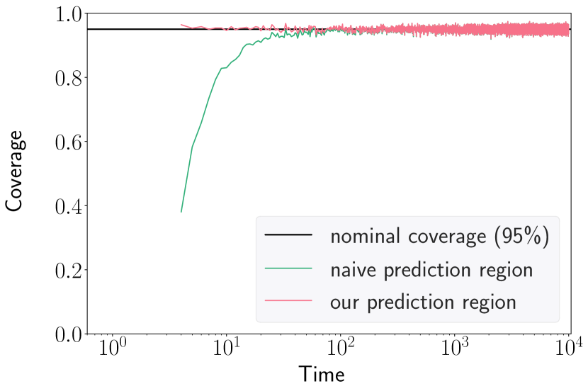
Note that the naive prediction region
| (17) |
also has asymptotically exact coverage even though it ignores the estimation error in . However, our experiments show that our prediction region from Eq. 16 achieves much better finite-sample coverage by accounting for the estimation error of ; see Figure 1(e).
4 Experiments
We verify our algorithm’s performance in one stable and one unstable dynamical system. We focus on comparing the finite sample performance of our algorithm to our theoretical predictions, and defer comparison between our algorithm and other existing algorithms for future work (see Dean et al., (2018) for a comparison between an algorithm similar to our algorithm except it updates logarithmically often and other algorithms which we will review in Section 5). In the main text, we will only display the figures with and in the stable system; the remaining figures and details of the experimental setup can be found in Appendix I. 555Source code for reproducing our results can be found at https://github.com/Feicheng-Wang/LQAC_code.
4.1 A representative simulation
Figure 2 summarizes the results of our experiment with and in a stable system (for the analogous figure in an unstable system see Figure I.2). The main takeaways are:
-
•
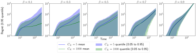
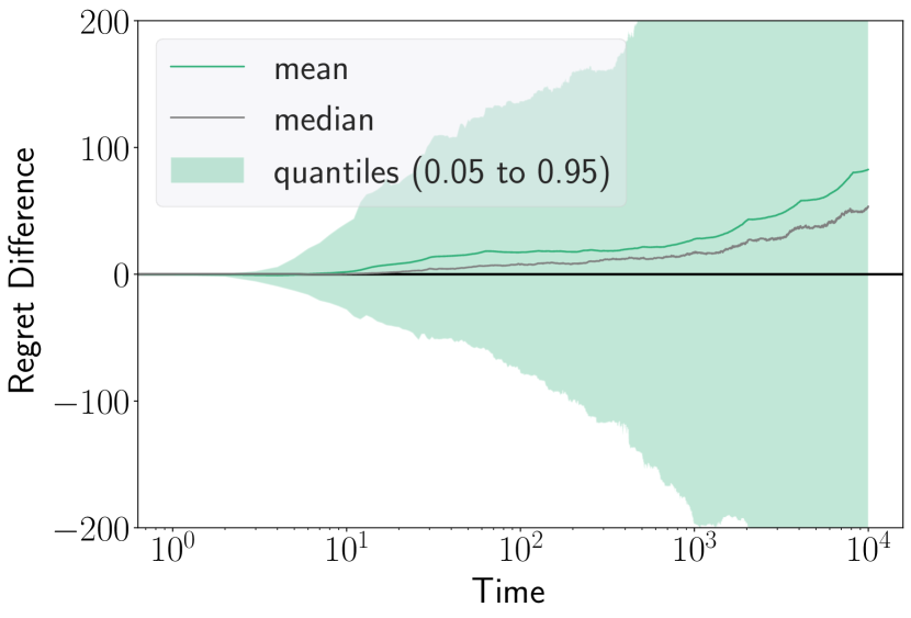
Figure 1(a) shows that Algorithm 1’s stepwise update leads to lower regret than update logarithmically often, although the difference is small compared with the variability of the regret. The difference is qualitatively similar but quantitatively larger in the unstable system, and the difference can be quite large for poor choices of , but pretty robust for choices of ; see Figures 1(a), I.3 and I.7.
-
•
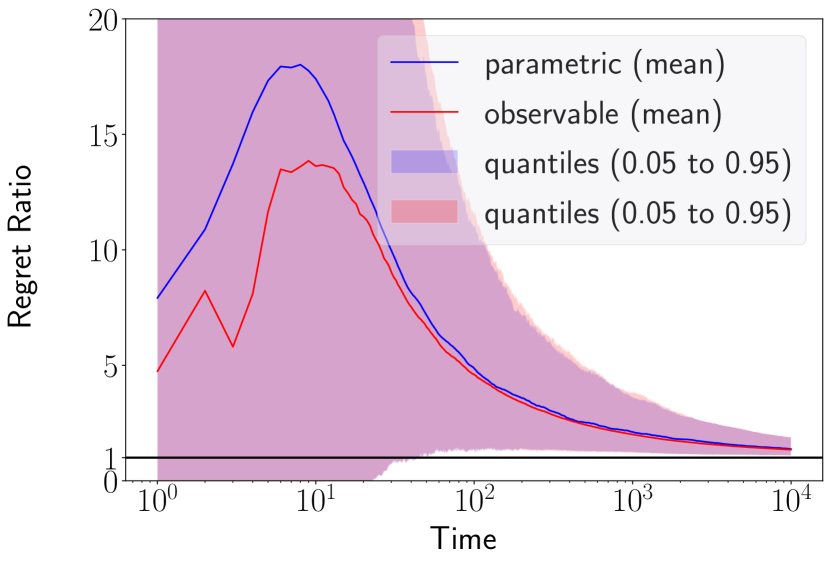
Figure 1(b) verifies that the ratio of the true observed regret with either of our regret expressions in Theorem 2 and Corollary 2 is converging to 1. Note that the large confidence band is due to the huge variance in the regret itself. The analogous plots for and the unstable system can be found at Figures 1(b) and I.4; larger speeds up the convergence speed.
-
•
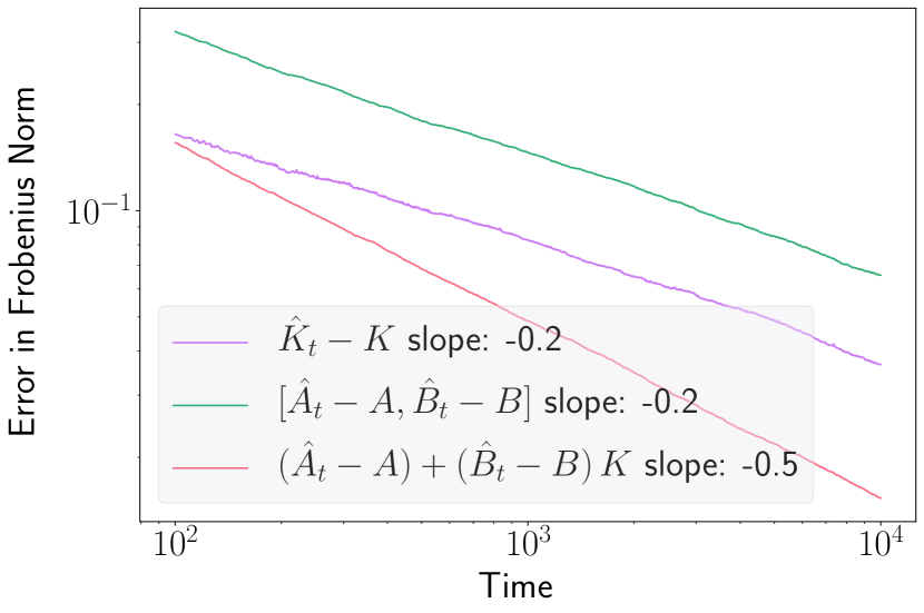
Figure 1(c) verifies the convergence rate disparity in Remark 2 that , , and have a slow convergence rate , while has a fast convergence rate ; see Figure 1(c).
-
•
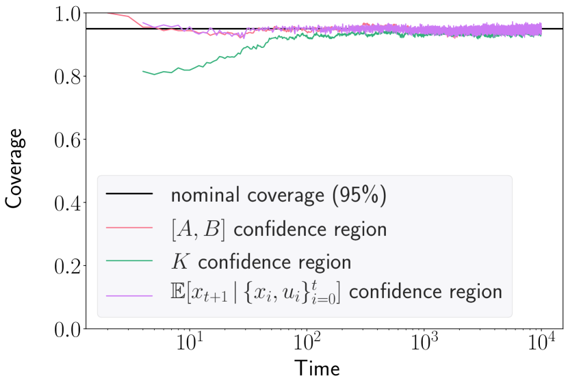
Figure 1(d) shows that, the finite sample coverage of our confidence regions and prediction region closely matches our asymptotic theory in Corollaries 3, 4 and 5. Also Figure 1(e) shows that our prediction region Eq. 16 have better finite sample coverage than the naive region Eq. 17. In this simulation, the observable expressions have slightly better coverage. Similar results hold for other choices of and the unstable systems (Figures 1(d) and I.6).
5 Detailed review of related work
The LQAC problem lies at the intersection of adaptive control and reinforcement learning and has drawn considerable attention in the past decade. This line of work differs from much of the work in reinforcement learning that is based on games or other virtual simulators that can be rerun infinitely many times (Vinyals et al., (2017), Silver et al., (2017)) because it is run in one-shot. However, many real-world applications cannot be easily restarted over and over again, and repeating experiments can be prohibitively expensive. Aside from the CE approach taken in this paper and reviewed in Section 1.3, we classify LQAC algorithms into two broad categories:
-
•
Optimism in the Face of Uncertainty: This method uses non-convex optimization to repeatedly select a near optimal control (in the regret sense) from a confidence set, achieves the optimal rate of regret (Abbasi-Yadkori and Szepesvári,, 2011; Ibrahimi et al.,, 2012; Faradonbeh et al.,, 2017). Later Cohen et al., (2019) extended this work by replacing non-convex optimization with semi-definite programming and still achieves the optimal regret.
-
•
Thompson Sampling: Starting with a prior distribution for the system parameters, one can use Bayes’ rule to update a posterior distribution online and can use samples from that posterior to choose controls that balance exploration and exploitation. The pioneering work (Abeille and Lazaric,, 2017) applying this idea to LQAC demonstrated a suboptimal average regret, which is later improved to the optimal rate by Ouyang et al., (2017); Faradonbeh et al., 2018b . Abeille and Lazaric, (2018) is the only work which we know of that achieves the optimal rate with stepwise updates, although their proofs only apply in scalar systems (i.e., ).
Logarithmic Regret
We pause here to clarify that any result achieving logarithmic regret is in a different setting from ours (in our setting, a lower bound of was proven in Simchowitz and Foster, (2020)). For example, when the system parameters and are known or partially known, a logarithmic rate of regret is achievable due to the extra information in and which allows faster estimation of (Foster and Simchowitz,, 2020; Cassel et al.,, 2020). Or, when the states are only partially observed, although the controller receives less information, the optimal controller also has less information, which turns out to allow a logarithmic rate of regret (Lale et al.,, 2020; Tsiamis and Pappas,, 2020). As a final example, when the cost is not an explicit function of the controls , a logarithmic rate of regret is achievable using a controller called a self-tuning regulator, which is similar to our certainty equivalent controller except that it targets a different optimal controller (because the cost function is different) and applies constant size probing steps logarithmically often (Lai and Wei,, 1986; Lai,, 1986; Guo and Chen,, 1991; Guo,, 1995).
Sequential Analysis and Time Series
Establishing asymptotic normality is common in sequential analysis (Lai,, 2001) and time series or state space model analysis (Kohn and Ansley,, 1986; Pedroni,, 2004), but the focus in these fields is on stationary and Markovian time series (although we assume our system is stabilizable, the data generated by applying our adaptive controller to that system is non-Markovian and non-stationary as the controller depends on the whole history) and on simpler forms of dependence than we consider.
6 Discussion
This paper’s main contributions are asymptotically exact expressions for the regret and the distributions of the estimation and prediction errors of a stepwise updating noisy certainty equivalent control algorithm in terms of either the system parameters or observable random variables. These results improve the field’s understanding of the LQAC problem and open up a number of new research directions:
-
1.
Theoretical improvements. Our simulations support our suspicion that all of our results except for Theorem 2 and Corollary 2 hold under more general version of Algorithm 1 that allows and , the summation in Line 4 to go up to , and the removal of Line 5. We expect such extensions to require significantly stronger theoretical machinery, and we hope that future work will prove these extensions and analogues to Theorem 2 and Corollary 2 which account for an expected additional term of order .
-
2.
Safe reinforcement learning. Existing work in safe reinforcement learning relies heavily on prediction regions derived from Bayesian inference (Berkenkamp et al.,, 2017; Koller et al.,, 2018). Our Corollary 5 provides a tight frequentist asymptotic prediction region that, unlike Bayesian inference, does not assume a prior on the system parameters, providing a potential starting point for new safe reinforcement learning algorithms.
-
3.
Non-stationarity reinforcement learning. As mentioned in the last paragraph of Section 3, our prediction region can be used for change point detection in non-stationary systems. Many existing work designed for reinforcement learning algorithms in the non-stationary environment relies on some form of change point detection, although they focus on discrete state and action spaces (Da Silva et al.,, 2006; Auer et al.,, 2009; Padakandla et al.,, 2019). Thus, our work may be useful for designing new reinforcement learning algorithms in non-stationary settings with continuous state and action spaces.
Acknowledgements
We are grateful to Na Li, Haoyi Yang, and Yue Li for helpful discussions regarding this project.
References
- Abbasi-Yadkori et al., (2011) Abbasi-Yadkori, Y., Pál, D., and Szepesvári, C. (2011). Online least squares estimation with self-normalized processes: An application to bandit problems. arXiv preprint arXiv:1102.2670.
- Abbasi-Yadkori and Szepesvári, (2011) Abbasi-Yadkori, Y. and Szepesvári, C. (2011). Regret bounds for the adaptive control of linear quadratic systems. In Proceedings of the 24th Annual Conference on Learning Theory, pages 1–26.
- Abeille and Lazaric, (2017) Abeille, M. and Lazaric, A. (2017). Thompson sampling for linear-quadratic control problems. In AISTATS 2017-20th International Conference on Artificial Intelligence and Statistics.
- Abeille and Lazaric, (2018) Abeille, M. and Lazaric, A. (2018). Improved regret bounds for thompson sampling in linear quadratic control problems. In International Conference on Machine Learning, pages 1–9.
- Anderson and Kunitomo, (1992) Anderson, T. W. and Kunitomo, N. (1992). Asymptotic distributions of regression and autoregression coefficients with martingale difference disturbances. Journal of Multivariate Analysis, 40(2):221–243.
- Auer et al., (2009) Auer, P., Jaksch, T., and Ortner, R. (2009). Near-optimal regret bounds for reinforcement learning. In Advances in neural information processing systems, pages 89–96.
- Becker et al., (1985) Becker, A., Kumar, P., and Wei, C.-Z. (1985). Adaptive control with the stochastic approximation algorithm: Geometry and convergence. IEEE Transactions on Automatic Control, 30(4):330–338.
- Berkenkamp et al., (2017) Berkenkamp, F., Turchetta, M., Schoellig, A., and Krause, A. (2017). Safe model-based reinforcement learning with stability guarantees. In Advances in neural information processing systems, pages 908–918.
- Bombois et al., (2006) Bombois, X., Scorletti, G., Gevers, M., Van den Hof, P. M., and Hildebrand, R. (2006). Least costly identification experiment for control. Automatica, 42(10):1651–1662.
- Cassel et al., (2020) Cassel, A., Cohen, A., and Koren, T. (2020). Logarithmic regret for learning linear quadratic regulators efficiently. arXiv preprint arXiv:2002.08095.
- Choi and Seo, (1999) Choi, J. W. and Seo, Y. B. (1999). Lqr design with eigenstructure assignment capability [and application to aircraft flight control]. IEEE Transactions on Aerospace and Electronic Systems, 35(2):700–708.
- Cohen et al., (2019) Cohen, A., Koren, T., and Mansour, Y. (2019). Learning linear-quadratic regulators efficiently with only regret. In International Conference on Machine Learning, pages 1300–1309.
- Da Silva et al., (2006) Da Silva, B. C., Basso, E. W., Bazzan, A. L., and Engel, P. M. (2006). Dealing with non-stationary environments using context detection. In Proceedings of the 23rd international conference on Machine learning, pages 217–224.
- Dean et al., (2018) Dean, S., Mania, H., Matni, N., Recht, B., and Tu, S. (2018). Regret bounds for robust adaptive control of the linear quadratic regulator. In Advances in Neural Information Processing Systems, pages 4188–4197.
- Dean et al., (2019) Dean, S., Mania, H., Matni, N., Recht, B., and Tu, S. (2019). On the sample complexity of the linear quadratic regulator. Foundations of Computational Mathematics, pages 1–47.
- Engel et al., (2004) Engel, Y., Mannor, S., and Meir, R. (2004). The kernel recursive least-squares algorithm. IEEE Transactions on signal processing, 52(8):2275–2285.
- Faradonbeh et al., (2017) Faradonbeh, M. K. S., Tewari, A., and Michailidis, G. (2017). Finite time analysis of optimal adaptive policies for linear-quadratic systems. arXiv preprint arXiv:1711.07230.
- (18) Faradonbeh, M. K. S., Tewari, A., and Michailidis, G. (2018a). Input perturbations for adaptive regulation and learning,”. arXiv preprint arXiv:1811.04258.
- (19) Faradonbeh, M. K. S., Tewari, A., and Michailidis, G. (2018b). On optimality of adaptive linear-quadratic regulators. arXiv preprint arXiv:1806.10749.
- Fazel et al., (2018) Fazel, M., Ge, R., Kakade, S., and Mesbahi, M. (2018). Global convergence of policy gradient methods for the linear quadratic regulator. In International Conference on Machine Learning, pages 1467–1476.
- Foster et al., (2020) Foster, D. J., Rakhlin, A., and Sarkar, T. (2020). Learning nonlinear dynamical systems from a single trajectory. arXiv preprint arXiv:2004.14681.
- Foster and Simchowitz, (2020) Foster, D. J. and Simchowitz, M. (2020). Logarithmic regret for adversarial online control. arXiv preprint arXiv:2003.00189.
- Gerencsér et al., (2009) Gerencsér, L., Hjalmarsson, H., and Mårtensson, J. (2009). Identification of arx systems with non-stationary inputs—asymptotic analysis with application to adaptive input design. Automatica, 45(3):623–633.
- Gerencsér et al., (2017) Gerencsér, L., Hjalmarsson, H., and Huang, L. (2017). Adaptive input design for lti systems. IEEE Transactions on Automatic Control, 62(5):2390–2405.
- Grünwald et al., (2019) Grünwald, P., de Heide, R., and Koolen, W. (2019). Safe testing. arXiv preprint arXiv:1906.07801.
- Guo, (1995) Guo, L. (1995). Convergence and logarithm laws of self-tuning regulators. Automatica, 31(3):435–450.
- Guo and Chen, (1991) Guo, L. and Chen, H.-F. (1991). The astrom-wittenmark self-tuning regulator revisited and els-based adaptive trackers. IEEE Transactions on Automatic Control, 36(7):802–812.
- Hautus, (1970) Hautus, M. (1970). Stabilization controllability and observability of linear autonomous systems. In Indagationes mathematicae (proceedings), volume 73, pages 448–455. North-Holland.
- Hjalmarsson, (2009) Hjalmarsson, H. (2009). System identification of complex and structured systems. In 2009 European Control Conference (ECC), pages 3424–3452. IEEE.
- Huang et al., (2012) Huang, L., Hjalmarsson, H., and Gerencsér, L. (2012). Adaptive experiment design for armax systems? In 2012 IEEE 51st IEEE Conference on Decision and Control (CDC), pages 907–912.
- Ibrahimi et al., (2012) Ibrahimi, M., Javanmard, A., and Roy, B. V. (2012). Efficient reinforcement learning for high dimensional linear quadratic systems. In Advances in Neural Information Processing Systems, pages 2636–2644.
- Jamieson et al., (2018) Jamieson, K., Ademola-Idowu, S. A., and Shi, Y. (2018). Lecture 20 : Linear dynamics and lqg 3 2 linear system optimal control 2 . 1 linear quadratic regulator ( lqr ) : Discrete-time finite horizon.
- Janson, (2011) Janson, S. (2011). Probability asymptotics: notes on notation. arXiv preprint arXiv:1108.3924.
- Khosravi and Smith, (2020) Khosravi, M. and Smith, R. S. (2020). Nonlinear system identification with prior knowledge of the region of attraction. arXiv preprint arXiv:2003.12330.
- Kohn and Ansley, (1986) Kohn, R. and Ansley, C. F. (1986). Prediction mean squared error for state space models with estimated parameters. Biometrika, 73(2):467–473.
- Koller et al., (2018) Koller, T., Berkenkamp, F., Turchetta, M., and Krause, A. (2018). Learning-based model predictive control for safe exploration. In 2018 IEEE Conference on Decision and Control (CDC), pages 6059–6066. IEEE.
- Lai, (1986) Lai, T. (1986). Asymptotically efficient adaptive control in stochastic regression models. Advances in Applied Mathematics, 7(1):23–45.
- Lai and Robbins, (1982) Lai, T. and Robbins, H. (1982). Iterated least squares in multiperiod control. Advances in Applied Mathematics, 3(1):50–73.
- Lai and Wei, (1986) Lai, T. and Wei, C.-Z. (1986). Extended least squares and their applications to adaptive control and prediction in linear systems. IEEE Transactions on Automatic Control, 31(10):898–906.
- Lai, (2001) Lai, T. L. (2001). Sequential analysis: some classical problems and new challenges. Statistica Sinica, pages 303–351.
- Lai and Wei, (1982) Lai, T. L. and Wei, C. Z. (1982). Least squares estimates in stochastic regression models with applications to identification and control of dynamic systems. The Annals of Statistics, 10(1):154–166.
- Lale et al., (2020) Lale, S., Azizzadenesheli, K., Hassibi, B., and Anandkumar, A. (2020). Logarithmic regret bound in partially observable linear dynamical systems. arXiv preprint arXiv:2003.11227.
- Ljung, (1997) Ljung, L. (1997). System Identification: Theory for the User. Pearson, 2nd edition.
- Mania et al., (2019) Mania, H., Tu, S., and Recht, B. (2019). Certainty equivalence is efficient for linear quadratic control. In Advances in Neural Information Processing Systems, pages 10154–10164.
- Ouyang et al., (2017) Ouyang, Y., Gagrani, M., and Jain, R. (2017). Learning-based control of unknown linear systems with thompson sampling. arXiv preprint arXiv:1709.04047.
- Oymak and Ozay, (2019) Oymak, S. and Ozay, N. (2019). Non-asymptotic identification of lti systems from a single trajectory. In 2019 American Control Conference (ACC), pages 5655–5661. IEEE.
- Padakandla et al., (2019) Padakandla, S., Bhatnagar, S., et al. (2019). Reinforcement learning in non-stationary environments. arXiv preprint arXiv:1905.03970.
- Payne and Silverman, (1973) Payne, H. and Silverman, L. (1973). On the discrete time algebraic riccati equation. IEEE Transactions on Automatic Control, 18(3):226–234.
- Pedroni, (2004) Pedroni, P. (2004). Panel cointegration: asymptotic and finite sample properties of pooled time series tests with an application to the ppp hypothesis. Econometric theory, 20(3):597–625.
- Priess et al., (2014) Priess, M. C., Conway, R., Choi, J., Popovich, J. M., and Radcliffe, C. (2014). Solutions to the inverse lqr problem with application to biological systems analysis. IEEE Transactions on control systems technology, 23(2):770–777.
- Sarkar et al., (2019) Sarkar, T., Rakhlin, A., and Dahleh, M. A. (2019). Finite-time system identification for partially observed lti systems of unknown order. arXiv preprint arXiv:1902.01848.
- Sattar and Oymak, (2020) Sattar, Y. and Oymak, S. (2020). Non-asymptotic and accurate learning of nonlinear dynamical systems. arXiv preprint arXiv:2002.08538.
- Shabaani and Jalili-Kharaajoo, (2003) Shabaani, K. and Jalili-Kharaajoo, M. (2003). Application of adaptive lqr with repetitive control for ups systems. In Proceedings of 2003 IEEE Conference on Control Applications, 2003. CCA 2003., volume 2, pages 1124–1129. IEEE.
- Silver et al., (2017) Silver, D., Schrittwieser, J., Simonyan, K., Antonoglou, I., Huang, A., Guez, A., Hubert, T., Baker, L., Lai, M., Bolton, A., et al. (2017). Mastering the game of go without human knowledge. Nature, 550(7676):354–359.
- Simchowitz and Foster, (2020) Simchowitz, M. and Foster, D. J. (2020). Naive exploration is optimal for online lqr. arXiv preprint arXiv:2001.09576.
- Simchowitz et al., (2018) Simchowitz, M., Mania, H., Tu, S., Jordan, M. I., and Recht, B. (2018). Learning without mixing: Towards a sharp analysis of linear system identification. In Conference On Learning Theory, pages 439–473.
- Stojanovic and Filipovic, (2014) Stojanovic, V. and Filipovic, V. (2014). Adaptive input design for identification of output error model with constrained output. Circuits, Systems, and Signal Processing, 33(1):97–113.
- Stojanovic et al., (2016) Stojanovic, V., Nedic, N., Prsic, D., and Dubonjic, L. (2016). Optimal experiment design for identification of arx models with constrained output in non-gaussian noise. Applied Mathematical Modelling, 40(13-14):6676–6689.
- Sun et al., (2020) Sun, Y., Oymak, S., and Fazel, M. (2020). Finite sample system identification: Optimal rates and the role of regularization. In Learning for Dynamics and Control, pages 16–25. PMLR.
- Tsiamis and Pappas, (2020) Tsiamis, A. and Pappas, G. (2020). Online learning of the kalman filter with logarithmic regret. arXiv preprint arXiv:2002.05141.
- Vinyals et al., (2017) Vinyals, O., Ewalds, T., Bartunov, S., Georgiev, P., Vezhnevets, A. S., Yeo, M., Makhzani, A., Küttler, H., Agapiou, J., Schrittwieser, J., et al. (2017). Starcraft ii: A new challenge for reinforcement learning. arXiv preprint arXiv:1708.04782.
- Wahlberg et al., (2010) Wahlberg, B., Hjalmarsson, H., and Annergren, M. (2010). On optimal input design in system identification for control. In 49th IEEE Conference on Decision and Control (CDC), pages 5548–5553. IEEE.
- Wang and You, (2020) Wang, H. and You, D. (2020). Online streaming feature selection via multi-conditional independence and mutual information entropy. International Journal of Computational Intelligence Systems.
- Zheng and Li, (2020) Zheng, Y. and Li, N. (2020). Non-asymptotic identification of linear dynamical systems using multiple trajectories. arXiv preprint arXiv:2009.00739.
Appendix A Preliminaries
A.1 Notation
Let us first review the definition of , and generalize the notation to contain relative constants , as well as introducing a new notation representing constant functions that we know exactly the order as well as the coefficient in front of the largest order term.
Definition 1.
Let and both be real valued function, and suppose is strictly positive for any large enough. Then
-
1.
if and only if , for any .
-
2.
if and only if and , for any .
-
3.
is a fixed function with regard to such that , and
-
4.
is a fixed function with regard to such that , and
-
5.
For a set of random variables and a corresponding set of constants , the notation
means that the set of values converges to zero in probability as approaches an appropriate limit. Equivalently, can be written as , where is defined as
-
6.
For a set of random variables and , where is almost surely non-zero, the notation
means that
-
7.
The notation
means that the set of values is stochastically bounded. That is, for any , there exists a finite and a finite such that,
-
8.
if for almost every , there exists a number such that . In other words, if there exists a random variable such that Equivalently,
-
9.
The notation
means that the set of values is stochastically bounded up to a constant order of . That is, for any , there exists a finite , a finite , and a finite such that,
All these definitions can be generalized to vectors or matrices with entry-wise definition. Without extra specification, all norms (for both vectors and matrices) are meant to be norm , i.e., operator-2 norm for the matrix.
Some relationships between these notations are worth keeping in mind: (see Eq.(7) and Eq.(8) in Janson, (2011))
| (18) |
| (19) |
To carefully track down the constant chosen manually, when we state order bounds like , should not contain variables such as which are set fixed when we prove high probability bounds but could be varying later, but could contain global constants such as , , , , , , dimension , and , , , that are fixed throughout the whole algorithm.
In order to differentiate from fixed constants, we denote as constant terms which could be potentially varying and only related with . That means for the same symbol in two different places, they can be different constants. One special symbol is which represents constant that does not rely on any parameters.
A.2 Extending results to
Although the main text only considered vanishing exploration noise (i.e., ), for completeness (and because it is straightforward to do so) we will also consider the case of and for all of our results.
A.3 Proof dependency tree
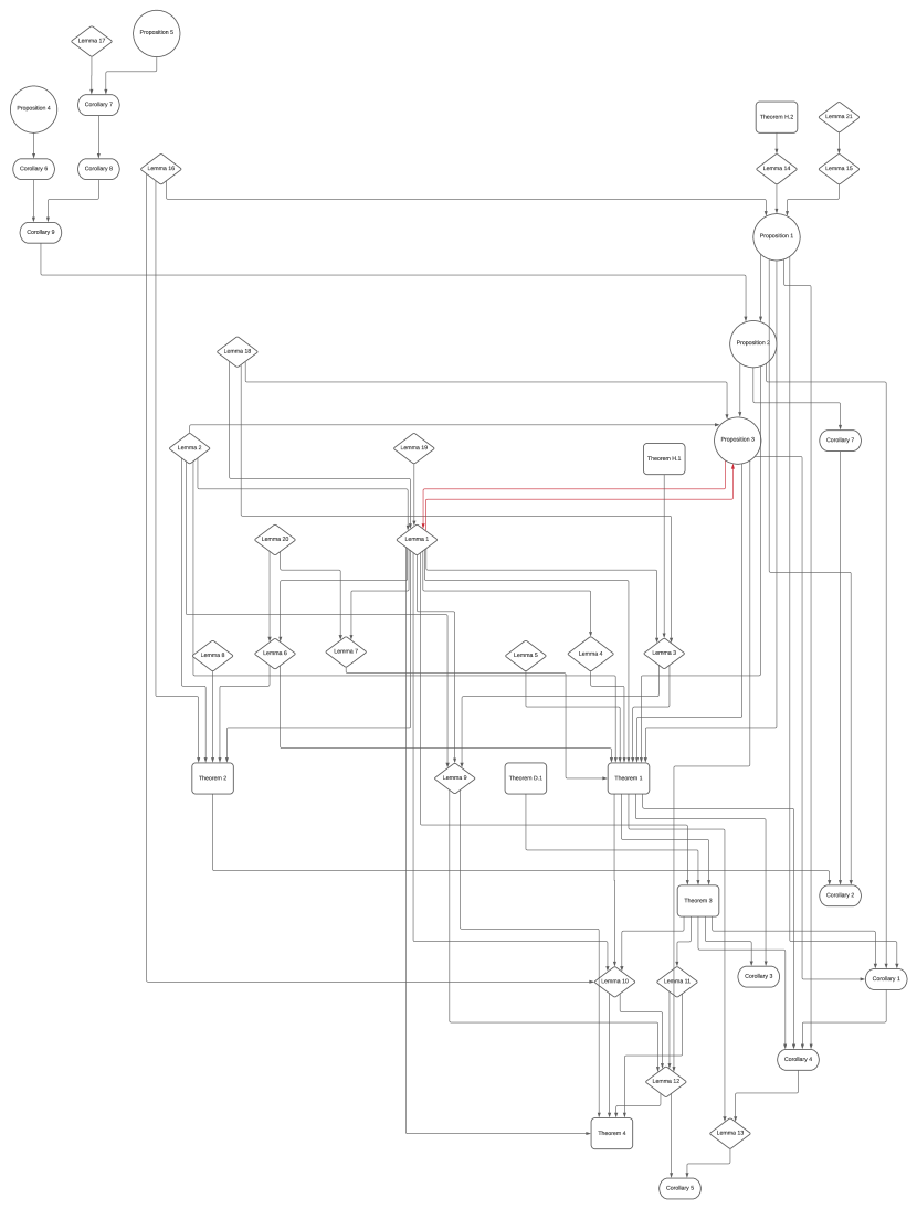
In order to make the proof more readable and easier to understand, we put the proof outlines first and summarize most useful middle steps by lemmas. These lemmas’ proofs often involve more technical details and is deferred to later parts in the appendix. While this may help readers have better understanding in the high level ideas behind the long proof, we realize that it may also cause loops in the proof structure. Thus, we provide a tree (Figure A.1) which describes the exact proof dependency structure to make sure that there is no circular argument. In Figure A.1, all conclusions lies in a perfect tree graph except for the loop marked in red between Lemma 1 and Proposition 3. This is not a contradiction because the proof of Proposition 3 only relies on a subset of conclusions in Lemma 1: Eqs. 24 and 25, which do not require Proposition 3 to hold. Some of the proofs relies on Eq. 81, which is not included in the graph but still self-consistent (does not rely on other results in the paper).
Appendix B The proof of Theorem 1
Theorem.
Algorithm 1 applied to a system described by Eq. 1 under Assumption 1 satisfies
| (20) |
B.1 Proof Outline
Proof.
Let us first examine the Gram matrix . Denote
| (21) |
and
| (22) |
We will show that
and thus we can write our Gram matrix as
Therefore, in order to satisfy
we can pick . is a deterministic matrix which satisfies and (we will give ’s exact expression in Eq. 29). With this choice of , we have
Components needing further explanation
In the final step of the above derivation there are still several points that remains unclear, namely
-
•
,
-
•
, and
-
•
.
As we will see, the order of is decided by the convergence rate of . Because of that, the first step in our proof is to identify the convergence rate of . Then we will prove the three remaining points in The proof of Eq. 20. To summarize, our proof can be mainly separated into two big steps:
-
1.
Identify the convergence rate of . (see Section B.2)
-
2.
Prove Eq. 20 holds:
-
•
Summarize uniform high probability bound for some random variables, which will serve as basic tools for later proof. (see Section B.3.1)
-
•
Prove . (see Section B.3.2)
-
•
Prove . (see Section B.3.3)
-
•
Prove . (see Section B.3.4)
-
•
Now we will examine these steps in order. ∎
B.2 Convergence rate of
As said in the previous part, the main purpose of this section is to derive the convergence rate of , which is one crucial step in our proof. Denote the stabilizing controller computed by Line 4 Algorithm 1 as , i.e.,
By Line 5 Algorithm 1, can be written as:
In particular, the proof can be separated into three parts:
-
1.
Derive the convergence rate of and .
-
2.
Show that enjoy the same convergence rate as and .
-
3.
Show that is only different from finitely often, and as a result, also enjoy the same convergence rate as and .
Correspondingly we have the following three propositions:
Proposition 1 (Similar to Proposition C.1 in Dean et al., (2018)).
Let be any initial state. Assume Assumption 1 is satisfied. When applying Algorithm 1,
The proof of Proposition 1 can be found in Section G.1.
Proposition 2.
Let be any initial state. Assume Assumption 1 is satisfied. When applying Algorithm 1,
The proof of Proposition 2 can be found in Section G.2.
Proposition 3.
Let be any initial state. Assume Assumption 1 is satisfied. When applying Algorithm 1,
| (23) |
The proof of Proposition 3 can be found in Section G.3.
Propositions 1, 2 and 3 all hold additionally for a version of Algorithm 1 that only updates logarithmically often; see Appendix G. The takeaway from this section is the uniform bound for Eq. 23, which is the only property of we need for the rest of the proof.
B.3 Proving Eq. 20
B.3.1 Uniform Bounds
In this section we will show several basic uniform bounds that will be used frequently in the later The proof of Theorem 1.
Lemma 1.
-
•
(24) -
•
(25)
Assume Eq. 23, then:
-
•
(26) -
•
For ,
(27) -
•
(28)
where , , and . Additionally, when all these terms are bounded by
The proof can be found in Section H.1.1. Following 1 Item 8, Lemma 1 presents uniform upper bounds for . We will see that all states and actions can be expressed in recursive summations, which can be bounded easily if we have uniform upper bound for each of their components.
Let us briefly explain why these orders makes sense.
-
•
The first two inequalities come from the tail bound for standard Gaussian random variables, whose maximum scales as .
- •
- •
-
•
The fifth inequality Eq. 28 holds because the system is stabilizable and the effect of previous states and actions are exponentially decaying, leaving the main factor in the norm to come from the recent system noises. By the first two inequalities is uniformly bounded by scale.
B.3.2 Showing
We wish to show that , where
| (29) |
Recall the system definition Eq. 1:
and the input Eq. 6
Recursively applying these two equations produces the following formula for in terms of , , and .
Lemma 2.
For any ,
| (30) |
and
Here when , we define the product .
The proof can be found in Section H.1.2. As a result, we can rewrite into a summation in terms of . First consider the terms without .
This whole expression can be separated into four components with the following bounds:
The proof can be found in Section H.1.3.
It remains to consider the remaining terms with , which is relatively straight-forward, since the effect of the initial state is exponentially decaying when .
Lemma 4.
Assume Eq. 23, then
-
1.
-
2.
The proof can be found in Section H.1.4. As mentioned in Eq. 19, notation is stronger than notation. Summing up all the results in Lemma 3 and Lemma 4 we can finally conclude that
Thus
| (31) |
where is defined in Eq. 29 This is already very close to our objective , but we still need to show that is an invertible matrix. is already a positive semi-definite (PSD) matrix because it is a weighted summation of PSD matrices and . The only thing we need to ensure is that is a full rank matrix. And that is indeed true because the term is the identity matrix, and adding more PSD matrices and will not change its positive definite nature. Following Eq. 29, we have (because or and )
| (32) |
Thus
| (33) |
Noticing that
we have from Eq. 31
| (34) |
With the help of the following lemma we conclude that .
Lemma 5.
Assume we have two matrix sequences and , where and are positive definite matrices, then
iff
The proof can be found in Section H.1.5 (Thanks for the help from Haoyi Yang and Yue Li in proving this lemma).
B.3.3 Proving
Lemma 6.
Assume Eq. 23, then
-
1.
-
2.
The proof can be found in Section H.1.6. The first term has larger order than the second term when or and . As a result, we have
| (35) | ||||
Observe from Eq. 33:
Then when or
B.3.4 Proving
Finally we need to check
where . There are six different kinds of terms in the above equation, namely , and , and , , and , and . The first three terms can be written as
and
The remaining terms can be summarized by
Lemma 7.
Assume Eq. 23, then
-
1.
-
2.
-
3.
The proof of Lemma 7 can be found in Section H.1.7. Combining all parts in Lemma 7 we have when or , the third item dominates the other two. To sum up, we have
| (36) |
Summary
Appendix C The proof of Theorem 2
Theorem.
The average regret of the controller defined by Algorithm 1 applied through time horizon to a system described by Eq. 1 under Assumption 1 satisfies, as ,
with therefore achieving the optimal rate (Simchowitz and Foster,, 2020) of .
C.1 Proof Outline
Proof.
We are interested in the cost
Notice that the state has the same expression as if the system had noise and controller . We wish to switch to the new system because there are some existing tools with controls in the form of .
We will first show in Section C.2 that the difference between the original cost and transformed cost is
and then prove in Section C.3 the new system cost is
Combining the above two equations, we conclude that
Based on similar analysis we prove in Section C.4 that
Recall that we choose , and when , which means is of larger order than . Finally we finish the proof with
∎
C.2 Cost difference induced by transformation
Next we consider the order of . Since ,
While the variance of is , which means the standard error is of lower order than the expectation. Thus
As a conclusion, the error caused by this transformation is of order , and the dominating term is .
| (37) |
C.3 Cost of transformed system
Next we proceed as if our system was with system noise and controller . The key idea of the following proof is from Appendix C of Fazel et al., (2018).
We are interested in the cost
which can be written as
| (38) |
We constructed the specific form of the first term on purpose. The following lemma translates the first term into a quadratic term with respect to .
Lemma 8.
For any with suitable dimension,
The proof can be found in Section H.2.1. As a result
Now we have three terms, and we will examine them in order.
- 1.
-
2.
The second term we consider is . Similar as before, we notice that . Then
Next consider
Thus
(39) -
3.
The third term we consider is . The expectation is
On the other hand, the variance is the sum of variances for each single summand with total order . As a result, when or
(40)
Summing up all three parts we have: when , or ,
| (41) |
Taking the transformation part into consideration (Eq. 37):
Finally we have when , or
Finally we only need to prove that the optimal average cost can be expressed as:
C.4 Optimal average cost
Appendix D The proof of Theorem 3
Theorem.
Algorithm 1 applied to a system described by Eq. 1 under Assumption 1 satisfies, as ,
Proof.
One can find the definition of in Eq. 7. The proof heavily relies on the following theorems from Anderson and Kunitomo, (1992). For better understanding, we directly state those theorems with the same notation as our paper.
Theorem D.1 (Theorems 1 and 3 in Anderson and Kunitomo, (1992)).
Let , , be a sequence of random vectors described by Eq. 1 under Assumption 1, and let be an increasing sequence of -fields such that is measureable and is measurable. Let the matrix be a deterministic matrix such that
| (42) |
where is a constant matrix, and
| (43) |
Suppose further that a.s., a.s.,
| (44) |
where is a constant positive semi-definite matrix and
| (45) |
as . Then
| (46) |
As we have seen in Algorithm 1 the controller is fully determined by . Pick
Now we verified the design vector at stage is measurable. Since , we know that , and is a martingale difference sequence with respect to an increasing sequence of -fields . Eq. 44 holds by the fact that all variances and Eq. 42. For Eq. 45, notice that we can remove the since every term has the same value, so the conclusion follows from a standard property of Gaussian distributions.
D.1 The proof of Eq. 43
Since
we have
| (48) | ||||
Recall that Eq. 43 is
It suffices to show
Actually we already shown in Lemma 1 that
This is a uniform bound over , thus a direct corollary is
That immediately implies
∎
Appendix E The proof of Theorem 4
Here we state and prove a generalization of Theorem 4 that allows for the case when and .
Theorem.
Algorithm 1 applied to a system described by Eq. 1 under Assumption 1 satisfies, as ,
| (49) |
Proof.
We can generalize the input noise to which is any random vector independent of the data before : . Hereafter, (but for is still ).
The proof will proceed by showing that acts as if it were independent of , and then effectively conditioning on and using ’s asymptotic distribution from Theorem 3.
Define as in Lemma 1. Define replacements of and which are independent of and :
| (50) |
and
| (51) |
We can show that the difference between and is very small:
Lemma 9.
The proof can be found in Section H.3.1. At the same time, the difference between , and is also small:
Lemma 10.
The proof can be found in Section H.3.2. These substitutions are very close to our original concern, and they have the good independence property:
This is because and are only functions of the system up to time , while and are independent with event before time by definitions in Eqs. 50 and 51. Our initial target is to identify the distribution of . We will start from its substitution
Because of this independence after substitution, the first term is independent with the second term, and their asymptotic distribution can be described by Eq. 11.
Lemma 11.
For any independent of the data before : :
The proof of Lemma 11 can be found in Section H.3.3. With the help of Lemma 9 and Lemma 10 , we can change all the replacements back to the original form:
Lemma 12.
For any independent of the data before : ,
The proof of Lemma 12 can be found in Section H.3.4. Since is independent with, which satisfies the condition of , we can restate the result with replaced by :
Finally, we have the desired conclusion using :
∎
Appendix F The proof of Corollaries
F.1 The proof of Corollary 1
Corollary.
Assume is full rank. Algorithm 1 applied to a system described by Eq. 1 under Assumption 1 satisfies
Proof.
Before we prove this result, we should first examine that the matrix is indeed invertible. Since has an identity matrix component , it is sufficient to show that is full rank.
F.1.1 is full rank
We can ignore the effect of and consider to be the same as certainty equivalent controller which is directly calculated by plugging into DARE Eqs. 3 and 4. This is because only happens finitely often and thus does not affect asymptotic properties; see Section G.3.
Before we start, we need to define how we solve and then prove that is indeed a full rank matrix. Lemmas 3.1 and B.1 from Simchowitz and Foster, (2020) gives the relationship between the derivatives of :
| (52) |
where can be solved from
| (53) |
Now we can solve by Eq. 52 and Eq. 53. Denote the kernel space of the derivative matrix as . It suffices to show that ’s dimension is , which implies is full rank with rank . The equivalent definition of kernel space is the small perturbation such that does not change ():
Any vector in kernel space can be considered as which satisfies in Eq. 52, and that means:
| (54) |
On the other hand, Eq. 53 describes a linear recursive relationship between and , so that we can solve with the infinite summation:
| (recursively plugging in the first equation) | |||
Also recall that is assumed to be full rank matrix, and we can show that is also full rank; see Section G.2. Thus we can explicitly solve from Eq. 54 as a linear equation with regard to :
This tells us the kernel space is the image of a function of its linear subspace , which means . Notice by kernel space definition its dimension should be at least , where the equality is achieved when has full rank . Combining these two equations we have . Finally we arrived at the desired conclusion that dimension of ’s kernel space is exactly , which means is full rank.
Next we describe the rest of the proof:
F.1.2 Proof by the Delta method
By Taylor expansion and the consistency of (see Proposition 1), we have
From Remark 2 we know
Then
which can be written as
By Eq. 11,
Combining the above two equations, finally we have
From the fact that is full rank and that has an identity matrix component , we can take matrix inverse and get
∎
F.2 The proof of Corollary 2
Corollary.
The average regret of the controller defined by Algorithm 1 applied through time horizon to a system described by Eq. 1 under Assumption 1 satisfies, as and ,
| (55) |
Proof.
This is a direct corollary from Theorem 2, which states
and from Proposition 1 and Corollary 7 which implies the consistency of and . By Slutsky’s theorem we can replace the parameters and in Eq. 55 with and . ∎
F.3 The proof of Corollary 3
Corollary.
Algorithm 1 applied to a system described by Eq. 1 under Assumption 1 satisfies
Proof.
For notational simplicity denote and . By Theorem 3 we know
| (56) |
Potentially we can derive an ellipsoid "confidence region" with the above formula by
| (57) |
However, since a true confidence region should not require any knowledge on oracle parameters, we need to replace with some observable expression, which turns out to be:
F.4 The proof of Corollary 4
Corollary.
Algorithm 1 applied to a system described by Eq. 1 under Assumption 1 satisfies
| (58) |
where is defined as evaluated at .
Proof.
Again, let us denote and . Starting from Theorem 3
we need to transfer to its observable version in terms of the Gram matrix. More specifically, we need to find another matrix which is observable and satisfies:
-
•
because we want to use Slutsky’s theorem.
-
•
because .
For now let us assume we have already found such matrix , and thus we can replace with :
That is:
Further denote , and then
| (59) |
By Taylor expansion and the consistency of (see Proposition 1), we have
Since we will prove in Section F.4.1, is asymptotically invertible, which means we can take inverse of in asymptotic equations:
We have already shown in Section F.1 that is full rank, in the same way we can prove that is almost surely full rank (the only difference is that we replaced with ). Recall the QR decomposition, we can re-express as , where is an invertible matrix, and satisfies . This implies that
From this and Eq. 59 we know
That is,
Recall that , and thus
By definition
Finally we can say
The only remaining task is to find a valid which satisfies and . Although we already have Theorem 1, is still not necessarily a valid choice, because we can only show is asymptotically an orthogonal matrix, but not identity matrix.
F.4.1 Finding a valid
Recall Eq. 36 that
Now denote
| (60) |
which is asymptotically proportional to the identity matrix, and is also symmetric. Recall that is defined as
We will verify that the following construction of is a valid choice:
We shall examine the two conditions and in order.
Proving
Proving
We will re-use the following equation later:
| (61) |
∎
F.5 The proof of Corollary 5
Corollary.
Algorithm 1 applied to a system described by Eq. 1 under Assumption 1 satisfies:
where for any independent of the data before : .
Proof.
This one final lemma connects Lemma 12 to our desired conclusion by changing the parametric expression to the observable one:
Lemma 13.
For any independent of the data before : ,
The proof of Lemma 13 can be found in Section H.3.5. Finally, we can say
∎
Appendix G The proof of Propositions
G.1 The proof of Proposition 1
Proposition (Similar to Proposition C.1 in Dean et al., (2018)).
Let be any initial state. Assume Assumption 1 is satisfied. When applying Algorithm 1,
G.1.1 Proof Outline
Proof.
We shall see that all the properties we derived in this section only require the safety condition Algorithm 1 Line 5 without any other requirement on the controller , and thus also apply to Algorithm 1 with logarithmic updates; see Remark 1.
According to Algorithm 1 Line 5, we keep our controller bounded , which means the next state can not be too far from the previous state. At the same time, whenever the state is too large (), it is tuned down by safe controller . Overall speaking, the state is always controlled with at most growth. We will see in Lemma 14 that when state growth is controlled, we have a decent bound on .
In other words, as long as we still run Algorithm 1 Line 5 at every time step, which is enough to "control" the system by itself, any generated with Line 4 satisfies
regardless of the estimation result before time .
Lemma 14 follows from a result by Simchowitz et al., (2018) on the estimation of linear response time-series. We present that result in the context of our problem. Let , and define . Then, the OLS estimator Eq. 5 is
| (62) |
We know that the accuracy of the OLS estimator is related to the covariance structure of the predictors, which are in our context. To capture such covariance structure, we need the following definiton:
Definition 2 (BMSB condition).
The -adapted process is said to satisfy the -block martingale small-ball (BMSB) condition if for any and , one has that
This condition is used for characterizing the size of the minimum eigenvalue of the matrix . A larger guarantees a larger lower bound of the minimum eigenvalue. In the context of our problem the result by Simchowitz et al., (2018) translates as follows.
Lemma 14 (A slightly different version of Theorem C.2 in Dean et al., (2018)).
For , for every , , , and such that satisfies the -BMSB and
| (63) |
the estimate defined in Eq. 62 satisfies the following statistical rate
| (64) |
The proof of Lemma 14 can be found in Section H.4.1.
We will show that grows linearly with (ignoring logarithmic terms), which means in Eq. 63 the LHS grows faster than the RHS, and is thus always satisfied if is large enough. Lemma 14 is saying that for any larger than some constant, we can control the norm of the system parameter estimate , which implies we can control the norm of both and .
Still there is one more gap from our Proposition 1, which requires uniform control on and . Fortunately, we have the blessing that this high-probability bound is in the log scale w.r.t . Because of that, we can choose a series of decaying for each different estimate , so that and we can achieve a uniform high probability bound on and for all , which directly leads to the desired conclusion once we plug in appropriate values for , , and :
To sum up, there are three main steps in our proof of Proposition 1:
∎
G.1.2 Verifying satisfies the -BMSB condition
In order to apply Lemma 14, we need to find , , and such that satisfies the -BMSB condition.
Lemma 15 (Similar to Lemma C.3 in Dean et al., (2018)).
If we assume Assumption 1, then apply Algorithm 1, the process satisfies the -BMSB condition for
where .
See Section H.4.2 for the proof of Lemma 15.
G.1.3 Upper bound of in terms of
The benefit of a non-random upper bound of w.r.t is two-fold.
Lemma 16 shows that we have an upper bound of that is .
Lemma 16 (Similar to Lemma C.4 in Dean et al., (2018)).
If we assume Assumption 1, then apply Algorithm 1, the process satisfies
| (65) |
See Section H.4.3 for the proof of Lemma 16.
G.1.4 Uniform upper bound for
With Lemma 15 and Lemma 16 in hand, we can translate Lemma 14 into our problem setting. Fixing , we already proved by Lemma 15 that the process satisfies the
| (66) |
If we choose and such that Eq. 63 holds with in Eq. 66, we can apply Lemma 14. By Eq. 65, we only need to satisfy
Since is growing faster than , the above condition is essentially saying that our should be larger than some constant . Suppose that is the case, then following Lemma 14 and Lemma 16, the estimate defined in Eq. 62 satisfies the following statistical rate
Notice that , and we know that . That is to say
Next we substitute , , , and into the previous equation
By merging all constant parameters in to the style expression, and noticing that , where , we have for any :
which implies
Notice that
Therefore we can derive a uniform confidence bound on the estimation error of parameters and : For any integer :
Notice that this is a uniform upper bound for all . Recall 1 Item 8, where we define as: for almost every , there exists a number such that , where denotes the sample space of . The previous equation is telling us the union of such event happens with at least probability , and by taking that is exactly the definition of , and thus:
The same bound holds for logarithmic updates. The reason is that for time , the closest estimation update will always be within time steps of , which does not change the order:
G.2 The proof of Proposition 2
Proposition.
Let be any initial state. Assume Assumption 1 is satisfied. When applying Algorithm 1,
G.2.1 Proof Outline
Proof.
When the problem parameters are known the optimal policy is given by linear feedback, , where and is the (positive definite) solution to the discrete Riccati equation
| (67) |
In the following context any time we mention and , we are refering to the corresponding certainty equivalent responses.
Since we already controlled the estimation error of and , one natural thing to ask is that, if we have control over and , do we have control over ? This can be achieved by two steps:
-
1.
Show that we can control once , , and are controlled.
-
2.
Show that we can control once and are controlled.
∎
G.2.2 Show that we can control once , , and are controlled
This is already stated by Proposition 1 in Mania et al., (2019). Denote the quantity
Proposition 4 (Proposition 1 in Mania et al., (2019)).
Let such that and . Also, let such that . Assume we have
The represents the minimum eigenvalue of . we can discard the constraint of by the following observation. If we replace our and by and , then the corresponding solution for Eq. 67 will be . Notice that changing and by the same proportion does not change the LQR problem. With that being said, our LS estimator , , and the nominal controller will remain the same. By this transformation the minimum eigenvalue condition is satisfied, and we only need to control
such that , and we will have , where . Here we can replace this denominator by any constant smaller than , and the whole story would still work. Since later we will also require , we can choose the shared denominator to be . To sum up we have the following corollary of Proposition 4.
Corollary 6.
Let such that and . Also, let such that . Then we have
where .
Now we only need to prove that given and .
G.2.3 Show that we can control once and are controlled
Consider a general square matrix . In order to quantify the decay rate of , we define
In other words, is the smallest value such that for all . We note that might be infinite, depending on the value of , and it is always greater than or equal to one. If is larger than , we are guaranteed to have a finite (this is a consequence of Gelfand’s formula). In particular, if is a stable matrix, we can choose such that is finite. Also, we note that is a decreasing function of ; if , we have .
Recall that . The following proposition that upper bounds holds in a more general LQG setting where the matrix is unknown:
Proposition 5 (Proposition 2 in Mania et al., (2019)).
Let and also let be such that , , and are at most . Let . We assume that , is stabilizable, observable, and .
as long as
Here are pure constants without dependence of any other parameters. We already assumed in Assumption 1 that stabilizable, but we have not defined ‘observable’ yet. An equivalent statement of observable can be found here.
Lemma 17 (Lemma 2.1 in (Payne and Silverman,, 1973)).
The pair is observable if and only if , imply
Since we already assumed is positive definite, imply , and thus is observable. In the LQAC setting we know exactly, so we can remove the estimation bound condition on .
Now we can restate Proposition 5 in the LQAC setting:
Corollary 7.
Let such that , and are at most . Let . We assume that , is stabilizable, and .
as long as
Here, the upper bound condition on is to ensure that is stabilizable, so that is well defined. Furthermore, following the paragraph after Proposition 2 in Mania et al., (2019), the assumption can be made without loss of generality when the other assumptions are satisfied. The reason is that, when and observable, the value function matrix is guaranteed to be positive definite. Similar to how we got Corollary 6, by replacing , and with , and , we can remove the constraint .
Corollary 8.
Suppose and . Let . We assume that and is stabilizable.
as long as
G.2.4 Combining the two results together
With Corollary 6 and Corollary 8 the following corollary is straightforward.
Corollary 9.
Let such that , and . Then, we have
Here .
Proof.
With Corollary 8 we can find such that . Thus, the condition of Corollary 6 is satisfied. ∎
G.2.5 Concluding the proof of Proposition 2
Proof.
With Proposition 1 and Corollary 9, it is straightforward to give a new corollary with uniform control on all , , and . Recall that we already proved the high probability bound in Proposition 1 that
Basically, to satisfy the constraint in Corollary 9, we only need our bound (named ) in Proposition 1 to satisfy
which is always true when is large enough. (This also ensures to be stabilizable so that is only used finitely many times.) That means,
Finally, we can say
∎
G.3 The proof of Proposition 3
Proposition.
Let be any initial state. Assume Assumption 1 is satisfied. When applying Algorithm 1
Proof.
Going thorough the whole Algorithm 1, there are two conditions that might cause the difference between and :
-
1.
, and
-
2.
.
Our objective is to show that, with probability , will happen only finitely often.
The first case
The first case is when , this will not happen infinitely often. The first case can only happen when
| (68) |
By Proposition 2, we know that is exponentially decaying:
As a result, Eq. 68 will hold only finitely many times, a.s.
The second case
To examine how often this would happen, we need to dig into more details of the decomposition of . Recall the previously derived formula from Lemma 2:
We hope to get an upper bound for . Apparently the main difficulty here is to bound the norm of . The following lemma serves as a key.
Lemma 18.
Suppose we have a constant square matrix with spectral radius , and a sequence of uniformly bounded random variables , satisfying . Denote the constant . Then we have, for any , :
And as a direct corollary
The proof can be found in Section H.5.1.
Notice that by our Algorithm 1, always holds, thus there exists a uniform upper bound on . Now we can separate the whole into two parts. If we denote , then with Lemma 18, we can simultaneously bound both parts.
-
1.
The first part contains the where , this part of product is denoted as . In this part, . Suppose this part has same items, by LABEL:{lem:productBound} we know
-
2.
The second part contains the where to be our true certainty equivalent controller, this part of the product is denoted as . If we denote , then, in this part, . Remember our conclusion in Proposition 2 that , thus , assuming this part has items, then since , by Lemma 18
We know . Combining these two parts we have
Finally we have the bound on :
Then
By Gaussian tail bounds (see Lemma 1), we know that
Then
Because is geometric sequence,
Thus for almost any , will happen only finitely many times.
Finally, because two conditions and will happen only finitely many times, and eventually are the same. Following Proposition 2,
∎
Appendix H The proof of lemmas
H.1 Lemmas in Appendix B
H.1.1 The proof of Lemma 1
Lemma.
-
•
(69) -
•
(70)
Assume Eq. 23, then:
-
•
(71) -
•
(72) -
•
(73)
where , , and . Additionally, when all these terms are bounded by
Proof.
Outline:
The proof of Eq. 69 and Eq. 70
The following lemma give the proof that Eq. 69 and Eq. 70 holds with probability at least , which can be shown by the tail bound for i.i.d Gaussian random variables.
Lemma 19.
For the noise and , we have that for any , with probability , the following two equations holds for any :
The proof of Eq. 71 and Eq. 72
Eq. 71 directly follows from Eq. 23. Eq. 72 follows from Lemma 18 given that we have from Proposition 3:
The proof of Eq. 73
The proof of Lemma 19
Proof.
For any Gaussian variable ,
and
For any multivariate normal vector sequence ,
That means for any constant ,
We can sum up all choices of to get a uniform bound. A well known equation states that . Then
We can choose , so that
That is to say, with probability at least , we have for any ,
Since can be dominated by , the above equation can simply be written as
This bound holds for which has constant variance and is also true for which has shrinking variance. Thus, with probability at least :
Consider the fact that , which means can still be bounded by:
∎
H.1.2 The proof of Lemma 2
Lemma.
Here when , .
Proof.
Consider the following relationship:
Iteratively do this calculation to the end:
∎
H.1.3 The proof of Lemma 3
Proof.
The first step is to show the order of 2nd, 3rd and 4th part because they follow by the same method, especially the second part is just a transpose of the third part. Then we can focus on analyzing the first part, which is replacing all controllers by optimal controller .
Second Part
With Lemma 1 in hand, now we are in good shape to start our proof with the second part showing
Since we have already shown the uniform bound of in Lemma 1, and that has an exponential decay rate, the main difficulty in bounding the second part is to give a tight bound on .
Recall the conclusion of Lemma 1:
| (74) |
Thus
| (75) |
Now the L2 norm of the second term can be bounded as
| (76) |
At first glance it seems like there is no way this would generate the desired bound, because the term could diverge when is large. However, thanks to the exponentially decaying term , we can avoid this by changing the order of summation:
| (77) |
The final form is almost the same as the beginning, except that the summation of disappears. Restart from Eq. 76, and remember to use Eq. 77 (Additionally, when , is meant to be ):
| (78) |
We know that for any matrix , , where is the rank of matrix . Thus Section H.1.3 implies an upper bound on the Frobenius norm, and the Frobenius norm implies entry-wise upper bound:
Third Part
This part is the transpose of the second part, thus shares the same result with the second part.
Fourth Part
Summarize second, third, and fourth parts
To sum up, all three parts are bounded by the same order
First Part
It remains to show
Recall . We divide the left hand side into two separate parts:
-
•
The part where . We will show this part is dominated by the part and is only of order .
-
•
The part where . We will show that
Let us first consider the part where . We will show the order of by considering its expectation and variance. Since is a summation of cross terms and , . Now it remains to consider the variance
It is sufficient to consider the first term in the previous expression, and the other term can be analyzed in exactly the same way. Notice the following relationship on any square matrix with dimension
That is
Then
Thus the entry-wise standard error of is of order . Combining this with the fact that , we have
| (79) |
and it remains to consider
Consider the expectation of : , where
Let us first show , and after that we only need to consider , which is the dominating term. We know that has a finite fourth moment, so the sum of the variances of each element of can be written as
Thus . Now we only need to focus on:
Again, when , should be considered as 1. Let us start from the identity matrix part .
Notice
Thus
On the other hand (when , is meant to be ),
| (80) |
Now it remains to calculate . Let us consider a more general case where and is any real number. It is clear that this summation goes to infinity when . Recall the Stolz–Cesàro theorem:
Theorem H.1 (Stolz–Cesàro).
Let and be two sequences of real numbers. Assume that is a strictly monotone and divergent sequence and the following limit exists:
Then, the limit
In Theorem H.1, we choose and to be and , respectively.
By Theorem H.1, we know
That is to say, for any :
| (81) | ||||
∎
H.1.4 The proof of Lemma 4
Lemma.
Assume Eq. 23, then
-
1.
-
2.
Proof.
This can be proved using a similar technique as in Section H.1.3. Recall that when , is taken to be .
Also,
∎
H.1.5 The proof of Lemma 5
Lemma.
Assume we have two matrix sequences and , where and are positive definite matrices, and
Then
Proof.
The basic idea is to utilize the equivalence of entry-wise convergence and F-norm convergence and the fact that the F-norm is invariant under orthogonal transformation. We know that positive definite matrices can be diagonalized by orthogonal transformation, and these diagonal matrices are easier to deal with. Starting from our only equation
Entry-wise convergence implies F-norm convergence:
By the positive definiteness of and , we can assume they have the diagnolization and , where and are diagonal matrices with diagonal values and (), and and are orthogonal matrices. With this transformation, we have
Since orthogonal transformation does not affect F-norm, on RHS inside the F-norm, we can multiply on the left and and on the right and get
Because F-norm convergence to zero is equivalent to entry-wise convergence to zero,
Denote , then
If we consider the th element of the above equation:
which is
Since by positive definiteness we have , the above equation implies
This holds for every pair. If we write out this equation back to matrix form, we would get
By the same trick this is equivalent to the F-norm form
On RHS inside the F-norm, we can multiply on the left and and on the right and get
Plug in our definition and :
And this implies
∎
H.1.6 The proof of Lemma 6
Lemma.
Assume Eq. 23, then
-
1.
-
2.
Proof.
First part
By Lemma 1 we have a uniform bound for and . We can derive the result in the first part by directly plugging in the bound for and .
By Lemma 1
Thus
which means (by bounding entry-wise terms by the operator norm)
Second Part
Following Lemma 2 (iii) from Lai and Wei, (1982):
Lemma 20.
Let be a martingale difference sequence with respect to an increasing sequence of -fields such that a.s. Let be an -measurable random variable for every . Then
And for any
As a result, with probability 1
| (82) |
We can apply Lemma 20 to our context by noticing
Here we normalized all to have a fixed normal distribution . Apply Eq. 82 entry-wise, where corresponds to a fixed entry of and corresponds to a fixed entry of . is bounded by . Thus
where . Applying the bounds in Lemma 1 (recall that when , is taken to be ):
Thus,
∎
In exactly the same way, we can show that
| (83) |
We first standardize
and then is bounded by
which is different from in by a constant factor . The rest of the proof is all the same.
H.1.7 The proof of Lemma 7
Lemma.
Assume Eq. 23, then
-
1.
-
2.
-
3.
Proof.
First part
Recall the conclusion from Lemma 1: and
This implies (by bounding the entries by the operator norm, and including the term as ):
Second part
The representative of the third term is . The proof idea is similar to that in Lemma 6 when we prove the bound for . Here we have an extra shrinking term which makes things easier.
Again, we can apply Lemma 20 to our context by noticing
Here we normalized all to have a fixed normal distribution. Apply Lemma 20 entry-wise, where corresponds to a fixed entry of and corresponds to a fixed entry of the normalized . Our is bounded by . Thus,
where . Apply the high probability bound in Lemma 1 and we have
That is to say, (adding the term as ). Thus,
Third part
By Eq. 81:
With a little abuse of notation we use as entry-wise variance of a matrix. Again, terms are meant to be .
When the last equation follows by Eq. 81 and when it is summation of harmonic series which is . Thus the standard error is only of order , which is smaller than . That is to say,
∎
H.2 Lemmas in Appendix C
H.2.1 The proof of Lemma 8
Lemma.
For any with suitable dimension,
H.3 Lemmas in Appendix E
H.3.1 The proof of Lemma 9
Lemma.
where
| (86) |
and
H.3.2 The proof of Lemma 10
Lemma.
Proof.
We can bound the distance of neighboring estimators by the following recursive LS formula. Denote , , . Then the LS estimator Eq. 5 is
For simplicity, denote , then our objective is to bound the difference .
As a result,
And
| (88) |
| (89) |
Next will bound the first and second term separately.
First term
Second term
Consider the variance of the -th element of , which is applicable to any choice of and . Fix , . Define as the filtration which contains every variable except for . We know that and .
Since , we have , which implies
By Eq. 89,
| (91) |
H.3.3 The proof of Lemma 11
Lemma.
For any independent of the data before : :
Proof.
We will start from finding the conditional distribution of
where and are constants. This should be easy because , which means we can directly apply the asymptotic normality result from Theorem 3. Recall Eq. 11 that
where (by Eq. 32). Here there are two different convergence speeds and we need to consider them separately. More precisely,
That is to say, for any constant vector and independent of data before , we have
The above equation holds because we are multiplying independent unit vector to the left hand side, so the result is still a normal distribution. Simplifying the equation:
We can replace with :
Because , we can drop the first three instances of :
Here we actually used the fact that for , when , then . This is because
In our specific context is the constant .
Since , we can replace with by conditioning on , replace all with , and finally remove the conditioning since they all converge in distribution to standard normal and asymptotically have same distribution.
| (92) | ||||
∎
H.3.4 The proof of Lemma 12
Lemma.
For any independent of the data before : ,
Proof.
Since we already proved Lemma 11, the only thing we need to do is to replace with , with , and , with , .
Replacing with
First, we can replace
with
Since is bounded away from with high probability ( has the component ),
By Lemma 9, . Recall Proposition 3 states that . Thus, the error induced by replacing the remaining with in Eq. 92 is
Under our condition or , this error is of order , which is negligible. Now we can replace all with :
Replacing by
Since (see Proposition 3), and , the final difference is still of order . Thus
Replacing , with ,
By Lemma 10,
Notice the and are multiplied by
thus their order is only . The difference induced by replacing with is of order . When or , this error is of order . Finally, after replacement we have
∎
H.3.5 The proof of Lemma 13
Lemma.
For any independent of the data before : ,
Proof.
Quadratic terms of
Let us first consider all those quadratic terms of :
-
•
-
•
-
•
Thus the later two items are dominated by the first term, and the quadratic terms of can be summarized by .
Quadratic terms of
That is already in a simple single item form, so we just keep it as .
Cross terms between and
Finally consider the cross terms of and :
which is dominated by the quadratic part. To sum up, we have
In other words
∎
H.4 Lemmas in Section G.1
H.4.1 The proof of Lemma 14
Lemma (A slightly different version of Theorem C.2 in Dean et al., (2018)).
Fixing , for every , , , and such that satisfies the -BMSB and
the estimate defined in Eq. 62 satisfies the following statistical rate
First let us review the main theorem in (Simchowitz et al.,, 2018). Lemma 14 is actually a corollary of that. To capture the excitation behavior observed in the case of linear systems we introduce a general martingale small-ball condition which quantifies the growth of the covariates for vectors (notice that this is different from 2).
Definition 3 (BMSB condition 2).
Given an -adapted random process taking values in , we say that it satisfies the -matrix block martingale small-ball (BMSB) condition for if, for any and ,
Theorem H.2 (Theorem 2.4 in Simchowitz et al., (2018)).
Fix , and . Then if is a random sequence such that (a) , where is -sub-Gaussian and mean zero, (b) satisfies the -small ball condition, and (c) such that . Then if
we have defined in Eq. 62 satisfies the following statistical rate
Now the main task is to translate this theorem to Lemma 14. First we need to derive the (a), (b), (c) three conditions from the assumptions in Lemma 14. Let us check the conditions one by one.
Condition (a)
Theorem H.2 states the model should be in the form of , where is -sub-Gaussian and mean zero. It is obvious that the system noise satisfy the sub-Gaussian and mean zero condition.
Condition (b)
satisfies the -small ball condition.
Condition (c)
We need to show that for some choice . Let us take
| (95) |
First we need to show that , and we can prove this from Eq. 94:
From a high level perspective, this equation allows us to have a lower bound on the minimum eigenvalue of , and then we can choose a small enough so that . By Markov inequality, for any ,
This is equivalent to
By Cauchy–Schwarz inequality:
Thus . By summing up this inequality with , we have
We can clean up the summation by merging and into one summation:
Recall that is any vector in , so the above equation can be translated into
This means
We wish to have so that and . One sufficient condition is
Next we need to show . For simplicity denote , which is a positive semi-definite matrix.
Result
Now that we verified all conditions of Theorem H.2, we can now translate the conclusion of Theorem H.2 into our setting. Theorem H.2 requires
First by our choice of and we have
| (96) | ||||
With this in hand, we know that
Notice that
Combining this with the previous inequality we have
H.4.2 The proof of Lemma 15
Lemma (Similar to Lemma C.3 in Dean et al., (2018)).
If we assume Assumption 1, then apply Algorithm 1, the process satisfies the -BMSB condition for
where .
Proof.
By 2 the statement means, for any and :
Recall that
Denote the filtration . It is clear that the process is -adapted.
Recall that is decided by in Algorithm 1, where our estimator is designed to be only dependent on , which means
For all , denote
Now we are ready to prove Lemma 15. We have
Given , only has randomness in , where is fixed given , and follows . That implies
Denote and as the mean and covariance of this multivariate normal distribution. Recall that we denoted . Let and then . Therefore,
| (97) | ||||
Here we used the fact that for any and , we have:
Recall in Algorithm 1, we force all our controllers to have norm , where is a constant. Then, by a simple argument based on a Schur complement (Lemma 21):
The desired conclusion directly follows:
∎
Schur complement
Lemma 21 (Lemma F.1 in Mania et al., (2019)).
Let be a positive-definite matrix and let be a real matrix. Then, for any we have that
H.4.3 The proof of Lemma 16
Lemma (Similar to Lemma C.4 in Dean et al., (2018)).
If we assume Assumption 1, then apply Algorithm 1, the process satisfies
Proof.
Now, note that
Since , we will show that if we can bound , then we can also get a bound for in the same order. Next we will focus on deriving the bound for .
Define . Since , there exists some integer that . Let us denote just for this Lemma 16.
For each , one of the following two statement must be true:
-
•
.
-
•
, which satisfies .
We can derive an upper bound for in both cases, and thus have an upper bound for every by adding up those two bounds in two different cases.
-
1.
If , recall that if , then we assert our controller in the next step to be probing noise: . By assumption we already had , for . That means we have a consecutive steps of probing noise with , for . Now we have
That is
which implies
(98) -
2.
If , which satisfies , then consider the following relationship
Therefore by our algorithm design that for any
(99)
By adding up Eqs. 98 and 99, we have a bound that is applicable to both cases. Notice our previous assumption that , where , further take , and to be all bounded by a constant for , which is of order (because ). By Eqs. 98 and 99
| (100) | ||||
Eq. 100 is very promising because it has a shrinking weight on . Let us use a simplified notation for the remainder:
In there are three types of components:
-
•
-
•
-
•
.
Since
| (101) |
we can control by
| (102) |
Now it only remains to show that is bounded by some constant. Notice that
By iteratively applying this inequality down to , we know that for :
Thus following from Eq. 103 we have
Since we already controlled the expectation of , it is straightforward to control the expectation of :
Thus,
| (104) |
Then we have
∎
H.5 Lemma in Section G.3
H.5.1 The proof of Lemma 18
Lemma.
Suppose we have a constant square matrix with spectral radius , and a sequence of uniformly bounded random variables , satisfying . Denote the constant . Then we have, for any , :
And as a direct corollary
Proof.
Our assumption of stability only says , but our analysis prefers similar exponential decay with regard to spectral norm. First, we need a conversion between spectral radius and spectral norm. Define
For simplicity, let us denote
and with Gelfand’s Formula
Thus is finite because . Since is uniformly bounded, we can assume an upper bound for . Let us now consider the spectral norm of .
Since , for every in the sample space , such that there exists some , whenever , , then
∎
Appendix I Experiment Details
I.1 Experiment Setting
I.1.1 Experiment Setting on Stable System
We set and , with system noise , injected noise baseline , , and initial state . As for the algorithmic hyper-parameters, we set the warning threshold for states at (so that ), the known stable controller , and the upper bound of the L2-norm for our controller at . Note that this is conservative by about a factor of 10, since the true optimal controller in this system is . Recall that the choice of these hyper-parameters does not actually affect our theoretical coverage (as long as ) or regret guarantees, but in practice their values prevent the system from incurring very large regret in the first few time steps. Even for this, they are only needed because we do not assume we are given an initial controller that is very close to ; in contrast, for instance, Dean et al., (2018) started from a controller fitted with 100 samples of white noise actions. All stable system results are based on 1,000 independent runs of Algorithm 1 for time steps.
I.1.2 Experiment Setting on Unstable System
The unstable system we simulate is highly unstable, and is largely the same as that in Appendix H of Dean et al., (2018). We set and , with system noise , injected noise baseline , , and initial state . As for the hyper-parameters, we set the warning threshold for states at (so that ), and we examined two different choices for the known stabilizing controller: and . The former choice incurs quite a bit higher regret than the latter, and hence we refer to the former as the ‘bad’ stabilizing controller and to the latter as the ‘good’ stabilizing controller. We set the upper bound of the L2-norm for our controller at the level of . Our choice of is different from the starting point in Dean et al., (2018), where they started from a burn in period estimate, and did not report the regret in the first 250 steps. All unstable system results are based on 1,000 independent runs of Algorithm 1 for time steps.
I.2 Experiment on Unstable System
In contrast to the stable system simulation summarized in Section 4.1, in this section we simulate the severely unstable system described in Section I.1.2. In this setting, the specification of is critical due to the costs incurred at the early time steps, an unavoidable consequence of starting from limited information in a system that can rapidly spiral (nearly) out of control.
I.2.1 Summary of results on unstable system
We begin with the analogue of Figure 2 for the unstable system, given in Figure I.2. The main takeaways are the same as the discussion in Section 4.1.
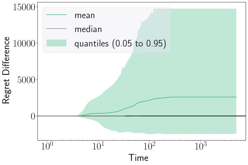
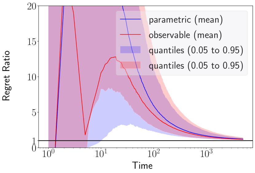
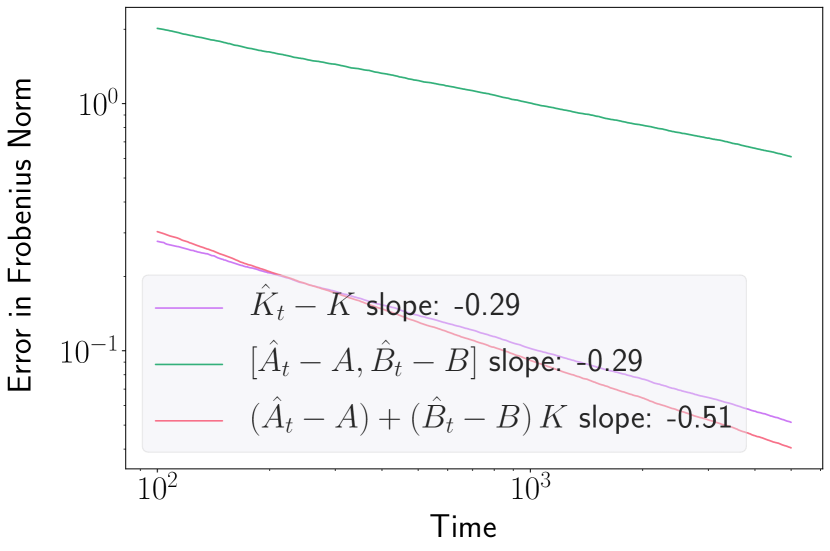
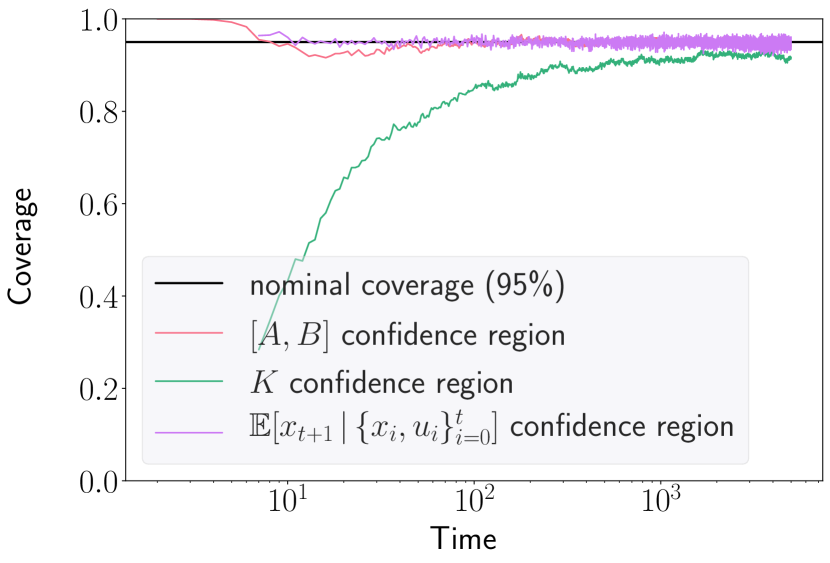
I.2.2 Large Regret From Early Time Steps
For the ‘bad’ choice of stabilizing controller , we plot the log regret in subplot (a) of Figure I.3. We observe a rapidly increasing regret in the first roughly 200 time steps, which dominates all the regret in the remaining steps. We offer a brief explanation why the cost in the early time steps is very large despite assuming knowledge of a stabilizing yet sub-optimal controller . Notice . Thus , , , , . So although we have a controlled system with maximum eigenvalue , the power of can still be very large in the bottom left corner for . Because of this, the randomness in the states is enlarged and propagated to several future steps. It turns out that, at the first 200 steps we used this high cost safety policy a lot as we do not have a good estimate of optimal controller , and that is the real reason for this high burn-in period cost. As we will see later, if we change the stabilizing controller to be closer to the optimal , the regret will be much smaller.
I.2.3 Comparison with Thompson Sampling
For comparison, we implement a straightforward version of Thompson sampling as follows. Denote . We use a prior of
Using the Bayesian updating equations and denoting the least-squares estimate of by , the posterior at time is given by
At each step, we draw a sample from this posterior and use it as the input to the DARE for calculating . Since a system is stabilizable if for any eigenvalue of (Hautus,, 1970), the Gaussian posterior puts probability 1 on stabilizable and hence defines a unique solution to the DARE with probability 1 as well.
We report the Thompson sampling regret in subplot (b) of Figure I.3, and see that it also suffers from rapidly increasing regret at early time points.f
I.2.4 Improved Regret When Using ‘Good’
When we switch from the ‘bad’ stabilizing controller to the ‘good’ one specified in Section I.1.2 as , we get that , which is a much better starting point than the previous , and the regret in this setting is indeed much better (see subplot (c) of Figure I.3) and resembles that of the stable system described in Section I.1.1.
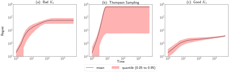
I.3 Choices of other than
Our simulations consider choices of beyond and even beyond those covered by our theory. In particular, we consider and observe promising evidence that some of our asymptotic coverage results may generalize to the setting of .
I.3.1 Regret
According to Theorem 2 the dominating term for regret should be for any and , and that indeed matches with our experimental results (see Figure I.4). The asymptotic regret expression from Theorem 2 is represented as the black solid curve, which converges to the empirical regret for , but not .
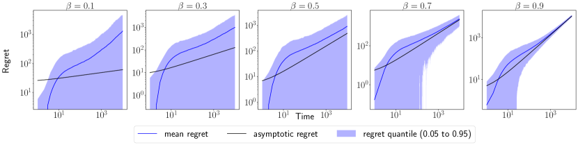
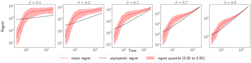
I.3.2 Confidence region coverage
Figure I.5 shows that the finite sample coverage of our confidence regions and prediction region closely matches the asymptotic theory from Corollaries 3, 4 and 5 for any choice among , with the exception of confidence regions for , which seem to only work for the covered by our theory.
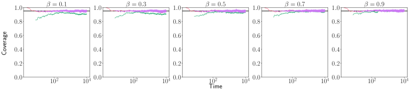
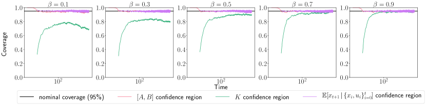
I.4 Algorithm design
We now investigate how the details of Algorithm 1 (the stabilizing controller and the thresholds on and ) impact the regret.
The threshold controls extreme tail behavior
Although we only trigger the threshold rarely, without it we can see some extreme behavior with low probability. In particular, when this threshold constraint is removed, we occasionally observe very large regret in early time steps due to the poor estimate , which causes instability of the system (see Figure I.6 and compare it to the purple line and shaded region in Figure I.7). The mean value is even higher than the 0.95 quantile curve because of several extremely large regrets induced by the unstable closed-loop system. And compared to when is used in Figure I.7, the 0.95 quantile when is not used is considerably higher, although its median is quite similar to the mean when is used.
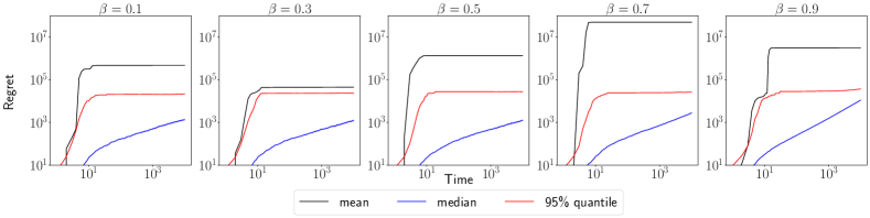
Stepwise updating improves regret over logarithmic updating
As our theory provides guarantees for Algorithm 1 with both stepwise and logarithmic updating, we run experiments to compare the regret of these two choices. Figures 1(c) and 1(c) show the difference in regret between Algorithm 1 and the same algorithm but that only updates its estimates of the system parameters logarithmically often, i.e., at times On average, we see a steady logarithmic increase in regret from switching from stepwise updates to logarithmic frequency.
A stabilizing controller closer to improves performance
Although is a stabilizing controller by assumption, bad choices of can still make large for some finite (see Section I.2.2 for a concrete example). Thus, unsurprisingly, choosing to be as near as possible to the optimal controller produces smaller regret, as evidenced by Figure I.3.
Regret is robust to conservative choices of
To check the sensitivity of the choice of in the stable system, we also tried a looser bound . We found that the norm of never surpassed the bound. This larger made little difference for settings covered by our theory (), and surprisingly seems to actually improve the regret for smaller (see Figure I.7).