Distributed Machine Learning for Computational Engineering using MPI

Abstract

We propose a framework for training neural networks that are coupled with partial differential equations (PDEs) in a parallel computing environment. Unlike most distributed computing frameworks for deep neural networks, our focus is to parallelize both numerical solvers and deep neural networks in forward and adjoint computations. Our parallel computing model views data communication as a node in the computational graph for numerical simulations. The advantage of our model is that data communication and computing are cleanly separated and thus provide better flexibility, modularity, and testability. We demonstrate using various large-scale problems that we can achieve substantial acceleration by using parallel solvers for PDEs in training deep neural networks that are coupled with PDEs.

1 Introduction

Inverse modeling [1, 2], which aims at identifying parameters or functions in a physical model from observations, is one key technique to solving data-driven problems in many applications. With the advent of deep learning techniques [3], we are now able to build neural-network-based data-driven models to solve inverse problems involving more complex physical phenomena. Specifically, by substituting unknown components within a physical system described by partial differential equations (PDEs) with deep neural networks (DNNs) [4, 5, 6, 7, 8] , we can leverage the expressive power of DNNs while satisfying the physics to the largest extent.

Gradient-based optimization algorithms [9, 10] are usually applied to train DNNs that are coupled with PDEs. A loss function, which measures the discrepancy between true and hypothetical observations, is minimized by iteratively updating DNN weights and biases. The gradients can be computed using automatic differentiation [11, 12, 13] and adjoint state methods [14]. In our previous work [15, 16, 5] , we have developed a general framework, ADCME, that expresses both DNNs and numerical PDE solvers (e.g., finite element methods) as computational graphs. Therefore, we can calculate the gradients automatically and with machine accuracy using reverse-mode automatic differentiation (AD). In ADCME, the automatic differentiation operates on a higher level of abstractions, such as tensor operations and matrix solvers, or even PDE solvers, instead of elementary ones (e.g., arithmetic operations) considered in general purpose AD software packages. This coarser granularity allows us to apply tensor-level performance optimizations and implement algorithms with a more intuitive and mathematical interface for scientific computing applications.

However, as the problem size grows, the memory consumption becomes prohibitive because reverse-mode AD requires saving all intermediate results. For example, a direct AD implementation of a 2D elastic equation double-precision solver with a mesh size $1000\times 1000$ and $2000$ steps requires at least 193 gigabytes memory [17], which is impractical for a typical CPU. Parallel computing using MPI [18, 19] is the de-facto standard for solving such a large-scale problem on modern distributed memory high performance computing (HPC) architectures. However, integrating a parallel computing capability into a reverse-mode automatic differentiation framework is challenging [20, 21, 22]. We need to back-propagate gradients through DNNs, numerical solvers, and control flows of parallel communications (Figure 1). These difficulties are magnified by the fact that we need the flexibility for hybrid threaded MPI capabilities (e.g., each MPI processor runs a multi-threading task and uses multiple cores on the same CPU) and therefore special efforts are needed to topological design of computational graph to avoid deadlocks.

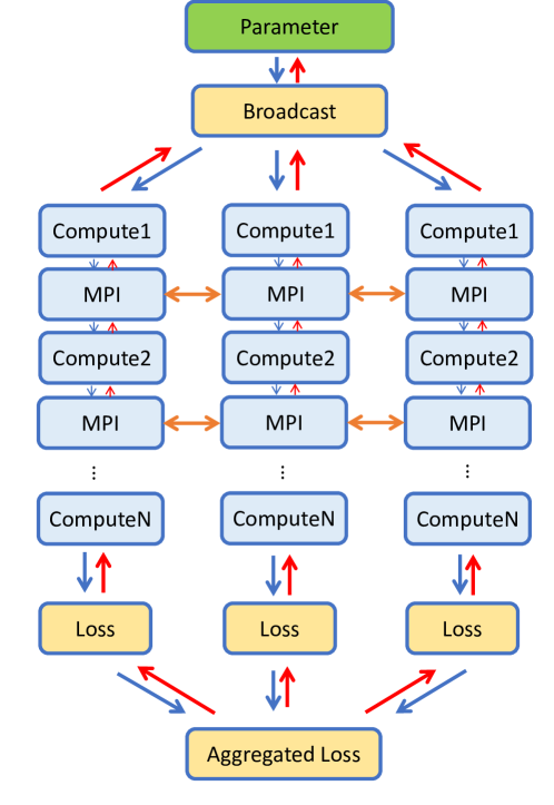
Figure 1: Parallel computational model for coupling DNNs and PDEs. There are two important data communication components: the parameters of DNNs are broadcasted to each MPI processor; within each MPI processor, there is data communication between adjacent patches in a computational grid.

Currently, distributed computing for reverse-mode AD have been intensively studied by two research communities: parallelizing numerical solvers [23, 24, 25] in scientific computing, and parallelized training (e.g., DNNs) [26, 27] in machine learning. In the scientific computing community, a computational grid is usually split into multiple patches and each MPI processor owns one patch. This allows to distribute degrees of freedoms onto different machines and thus relaxes the memory demands. Examples include libadjoint [28, 29] and DAfoam [30]. However, these frameworks are domain specific and are tightly integrated into dolfin [31] and OpenFOAM [32], respectively. This integration makes them difficult to adapt for general purpose data-driven inverse modeling, especially when deep neural networks are present and coupled with PDEs. In the machine learning community, one popular model is data-parallelism distributed computing [33], where each machine has full information of a complete DNN but only a portion of training data [34]. These DNNs share the same parameters, through a synchronization mechanism such as parameter servers (Figure 2) [35]. In these cases, the computations are mostly independent and there is no communication among different processors within each computational graphs. There are also the so-called model-parallelism distributed computing, in which DNNs themselves are split onto different machines [36]. However, these methods eventually lead to asynchronous training, where the correctness of gradients or the convergence is not guaranteed. Note that the distributed computing models from both two communities are quite different and are designed to meet their own needs. To couple DNNs and PDEs, where both synchronization of DNN parameters and parallel PDE solvers are present, a new distributed computing model that combines their features is desirable.

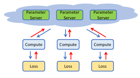
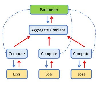
Figure 2: Left: parallelism via parameter servers. Each processor requests and updates states from the parameter servers. Parameter servers are responsible for maintaining the global states by communication within parameter servers themselves. Right: this paralell model can be viewed as a simplified version of parameter servers, where a master node collects all gradient information from other worker nodes.

In this work, we propose a novel framework for developing MPI-based distributed reverse-mode AD algorithms for coupling DNNs and PDEs. We consider treating data communication within both PDE solvers and DNN updates as nodes (operators) in the computational graph (Figure 3). These operators are non-intrusive to the other operators in the sense that existing implementation of the latter operators also works for parallel execution. The clean separation of data communication and computing offers the flexibility of reusing the existing ADCME framework and having the same implementation for both serial and parallel computing environments.

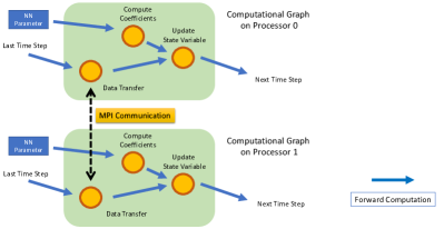
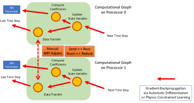
Figure 3: Paradigm for distributed machine learning for computational engineering. The data communication operations are treated as nodes in the computational graph. They are cleanly separated from other computing operators and therefore we can reuse serial implementations of the numerical PDE solver.

We use the high level language Julia [37] to specify the dependency of data communication operators and other computation operators. These data communication operators can be either built-in ADCME operators (e.g., mpi_bcast, which broadcasts a tensor to all workers), or provided by users in the form of custom operators. All computation and data communication are delegated to C++ or CUDA kernels at runtime, and the correctness of parallel programs is ensured by the topology of the computational graph. The MPI capability of ADCME relieves us from reasoning about the order of MPI calls, e.g., carefully ordering sends and receives to avoid deadlocks, and parallel communication rules for AD, e.g., forward sends become backward receives. Therefore, ADCME allows us to manage complex numerical simulations and accelerate development cycles. The separation of data communication and computation operators also allows us to test, analyze, and optimize them individually.

The aim of this paper is to describe the mechanism underlying ADCME MPI-based distributed computing capability. We also apply the tool to compute DNN gradients in a coupled system of DNNs and PDEs, such as Poisson’s equations and wave equations. We also present some important operators and data structures for scientific computing. For example, we use Hypre [38] as the distributed sparse linear solver backend and use CSR formats (mpi_SparseTensor) for storing a sparse matrix on each machine. In gradient back-propagation, the transpose of the original matrix is usually needed and such functionalities are missing in Hypre as of September 2020. The transposition is implemented as a separate operator in ADCME. The numerical examples demonstrate that ADCME can scale up to thousands of cores and solve large-scale scientific machine learning problems.

2 Distributed Scientific Machine Learning

2.1 Machine Learning for Computational Engineering

As an example, we consider the Poisson’s equation with a spatially varying diffusivity coefficient $\kappa(\mathbf{x})$:

$$\nabla\cdot(\kappa(\mathbf{x})\nabla u(\mathbf{x})) =f(\mathbf{x}) \mathbf{x}\in\Omega$$ (1)

$$u(\mathbf{x}) =0 \mathbf{x}\in\partial\Omega$$

Here $f(\mathbf{x})$ is a given source function, and $\Omega$ is a domain in $\mathbb{R}^{d}$. Assume that we can observe the state variable $u(\mathbf{x})$ at some locations $\{\mathbf{x}_{i}\}_{i\in\mathcal{I}}$, denoted as $\{u_{i}\}_{i\in\mathcal{I}}$, where $\mathcal{I}$ is the index set. We want to estimate $\kappa(\mathbf{x})$, whose form is in unspecified, from the observations.

This inverse problem can be formulated as an optimization problem

$$\min_{\kappa\in\mathcal{K}}\sum_{i\in\mathcal{I}}\left(u(\mathbf{x}_{i})-u_{i}\right)^{2}$$ (2)

Here $u(\mathbf{x}_{i})$ are the solutions to Equation 1 for a given $\kappa(\mathbf{x})$, and $\mathcal{K}$ is an appropriate function space for the unknown $\kappa$.

However, Equation 2 is typically an infinitely dimensional optimization problem if $\mathcal{K}$ cannot be parametrized by parameters with a finite dimension. To solve it numerically, we can approximate $\kappa$ with a deep neural network

$$\kappa(\mathbf{x})\approx\mathcal{N}_{\theta}(\mathbf{x})$$

where $\theta$ is the neural network weights and biases. This approach has been shown to be very effective, especially when $\kappa$ is a high dimensional mapping or lacks smoothness [39], compared to traditional approaches such as piecewise linear functions. Additionally, DNN representation also provides regularization thanks to its spatial correlation (e.g., if $\mathbf{x}_{1}$ and $\mathbf{x}_{2}$ are close, $\kappa(\mathbf{x}_{1})$ and $\kappa(\mathbf{x}_{2})$ are also close) and appropriate initialization.

Therefore, the optimization problem is reduced to a finite dimensional optimization problem, where the optimization variable is the DNN parameters:

$$\min_{\theta} \;J(\theta):=\sum_{i\in\mathcal{I}}\left(u(\mathbf{x}_{i})-u_{i}\right)^{2}\qquad(u(\mathbf{x}_{i})\text{ is an indirect function of }\theta)$$ (3)

s.t. $$\;\nabla\cdot(\mathcal{N}_{\theta}(\mathbf{x})\nabla u(\mathbf{x}))=f(\mathbf{x})\qquad\mathbf{x}\in\Omega$$

$$\;u(\mathbf{x})=0\qquad\mathbf{x}\in\partial\Omega$$

The PDE constraint in Equation 3 can be numerically solved using finite difference methods (or finite element methods), which results in a linear system

$$\mathbf{A}\mathbf{u}=\mathbf{f}$$ (4)

Here $\mathbf{u}\in\mathbb{R}^{n}$, $\mathbf{f}\in\mathbb{R}^{n}$, $\mathbf{A}\in\mathbb{R}^{n\times n}$, and $n$ is the degrees of freedoms. The reconstructed numerical solution $u(\mathbf{x})$ depends on $\theta$, although in general, we can not find an explicit expression for $u(\mathbf{x})$ with respect to $\theta$.

To solve the optimization problem Equation 3, we will calculate the gradients $\nabla_{\theta}J(\theta)$. In the context of reverse-mode automatic differentiation, this calculation requires us to back-propagate gradients through both the numerical solver and the neural network. In our previous work, we proposed a general framework for expressing both numerical simulations and DNNs as computational graphs, and thus unified the implementation of reverse-mode AD for deep neural networks and numerical solvers. This technique enables us to easily extract gradients $\nabla_{\theta}J(\theta)$ by reverse-mode automatic differentiation.

2.2 Parallel Computing

One challenge associated with reverse-mode AD is that all intermediate variables must be saved for gradient back-propagation. This requires additional memory compared to forward computation. Large-scale problems bring another difficulty to memory costs: we may not be able to solve even the forward problem, because it is challenging to save a large-sized discrete solution $\mathbf{u}$ on a single CPU.

One solution to ensure performance and scalability of numerical solvers is MPI. When we use MPI to solve Equation 3, the grid is split into multiple patches, and each machine (an MPI processor) owns one patch. We can rearrange the indices so that each MPI processor owns a stripe of rows in the matrix $\mathbf{A}$ and a segment of $\mathbf{f}$ with continuous indices. We resort to a distributed solver (e.g., from Hypre [38]) to solve the linear system Equation 4. After solving the linear system, each patch owns a segment of $\mathbf{u}$, and a local loss function can be computed. The local loss functions are then aggregated to calculate the global loss function.

However, when we compute the gradients, reverse-mode automatic differentiation with MPI is challenging because reasoning about reverse rules is difficult while avoiding deadlocks, ensuring correctness, and improving performance. There are many researches that focus on adjoint MPI [30, 40]. Many of them are tightly coupled with a specific application, and/or are not developed in the context of DNNs and PDEs.

Note that there are also active research in the deep learning community for distributed computing of DNNs. However, the parallel models are usually data-parallelism and do not consider communication within layers. For model parallelism in DNNs [41], usually DNNs are split into several parts and an asynchronous training method is used. These models are not appropriate for the inverse modeling problems that we are considering because communication does not happen within computational graphs. Instead, in our parallel model, the data communication pattern is more complicated: the data communication may occur multiple times within the computational graph, e.g., while performing time-stepping schemes or accumulating the loss function, etc. This difference calls for a new parallel model for both forward computation and gradient back-propagation.

3 Distributed Computing Design in ADCME

3.1 Basic MPI Operators

ADCME provides a subset of the MPI routines to facilitate implementing computational graphs with data communication capabilities. Most of the routines have gradient back-propagation capabilities. For example, the mpi_gather function corresponds to MPI_Gather, except that mpi_gather is differentiable. Internally, this API is implemented by observing that the scatter operation is the reverse of the gather operation in an MPI program. We show an excerpt from the mpi_gather implementation in ADCME:

⬇

void MPIGather_forward(double *out, const double *a, int m, int root){

MPI_Comm comm = MPI_COMM_WORLD;

MPI_Gather( a , m , MPI_DOUBLE , out , m , MPI_DOUBLE , root , comm);

}

\parvoid MPIGather_backward(

double *grad_a, const double *grad_out,

const double *out, const double *a, int m, int root

){

MPI_Comm comm = MPI_COMM_WORLD;

MPI_Scatter( grad_out , m , MPI_DOUBLE , grad_a , m , MPI_DOUBLE , root , comm);

}

Here MPIGather_forward implements the forward computation, and broadcast a from the root to all worker nodes buffers out. MPIGather_backward is the corresponding gradient back-propagation implementation. Having received grad_out from the downstream of the computational graph, this mpi_gather operator back-propagates the gradient to grad_a by reversing MPI_Gather. Table 1 presents parts of the built-in MPI operators in ADCME.

Table 1: MPI routines in ADCME. Many operations can perform both forward computation and gradient back-propagation. “YES” indicate that the operator supports gradient back-propagation.

API	Description	Gradient
mpi_init	Initialize an MPI session	NO
mpi_finalize	Finalize an MPI session	NO
mpi_initialized	A boolean indicating whether an MPI session is initialized	NO
mpi_finalized	A boolean indicating whether an MPI session is finalized	NO
mpi_rank	Current processor rank	NO
mpi_size	Total number of processors	NO
mpi_sync!	Broadcast a Julia array on all processors	NO
mpi_sum	Sum a tensor on the designated processor	YES
mpi_bcast	Broadcast a tensor from thedesignated processor	YES
mpi_recv	Receive a tensor from a given processor	YES
mpi_send	Send a tensor from a given processor	YES
mpi_sendrecv	Send a tensor from a given processor to another given processor	YES
mpi_gather	Concat tensors from all processors on the root processor	YES

As an example on how to use these primitive operators, consider computing

$$L(\theta)=1+\theta+\theta^{2}+\theta^{3}$$ (5)

The parameter $\theta$ is first broadcasted onto 4 processors using mpi_bcast. Processor $i$ computed $\theta^{i}$ locally. Then the results are summed on the root processor using mpi_sum. An ADCME program is as follows (Figure 4)

⬇

using ADCME

mpi_init() # initialize MPI

theta0 = placeholder(1.0)

theta = mpi_bcast(theta0)

l = theta^mpi_rank()

L = mpi_sum(l)

# initialize a Session

sess = Session(); init(sess)

L_value = run(sess, L) # only the value on rank 0 is valid

mpi_finalize() # finalize MPI

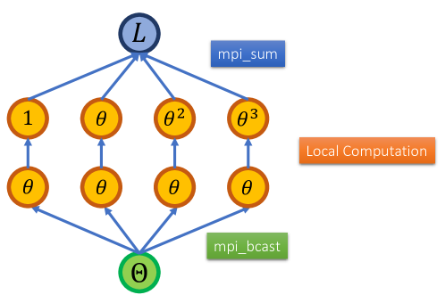
Figure 4: An illustration for computing Equation 5. $\theta$ is broadcasted onto 4 MPI processors. Local computing is then performed on each processor. Finally, the function values are aggregated via mpi_sum.

Additionally, we can use the following one-liner to extract gradients

⬇

grad = gradients(L, theta0)

This simple line of code hides the details for back-propagating gradients through local operations as well as MPI routines (mpi_bcast, mpi_sum).

3.2 Halo Exchange

In many applications, we use domain decomposition to distribute the workload onto different processors. To reduce the data communication overheads, subdomains usually overlap at the boundaries and exchange boundary data with their adjacent subdomains (Figure 5). This communication pattern is referred to as halo exchange. Halo exchange allows for communicating only a small portion of data compared to the data used for stencil computation within the subdomain. Halo exchange appears in many applications, and thus is implemented as a standalone operator in ADCME.

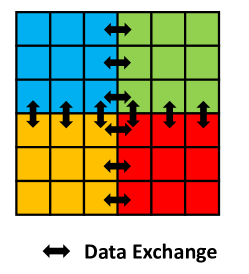
Figure 5: Domain decomposition and halo exchange. Two adjacent patches exchange boundary information.

The implementation of forward computation of halo exchange is straightforward. A direct application of blocking sends and receives will cause deadlocks. Instead, we use nonblocking sends and receives (Figure 6). For the reverse mode, the communication is also reversed for gradient back-propagation. The idea is that the forward sends correspond to reverse receives and the forward receives correspond to reverse sends. Additionally, the order should also be reversed. Once we work out the one-by-one substitution, the algorithm will work out correctly.

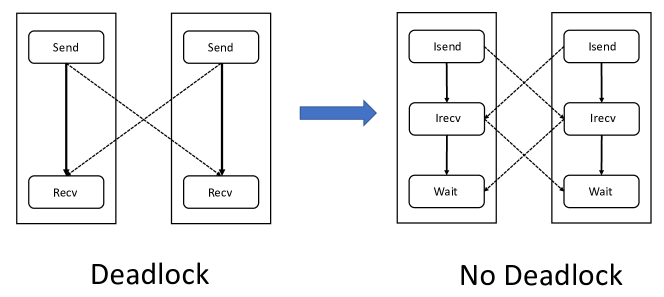
Figure 6: Avoid deadlocks using nonblocking sends and receives. Here Isend and Irecv are non-blocking sends and receives.

3.3 Distributed Sparse Matrices

ADCME uses Hypre as the distributed linear algebra backend for MPI matrix solvers. Each MPI processor owns a stripe of rows with continuous indices. The local matrix is stored in CSR (compressed sparse row) format and ADCME provides an interface mpi_SparseTensor to hide the implementation details.

For reverse-mode automatic differentiation, matrix transposition is an operator that are common in gradient back-propagation. For example, assume the forward computation is ($\mathbf{x}$ is the input, $\mathbf{y}$ is the output, and $\mathbf{A}$ is a matrix)

$$\mathbf{y}=\mathbf{A}\mathbf{x}$$ (6)

Given a loss function $L(\mathbf{y})$, the gradient back-propagation calculates

$$\frac{\partial L(\mathbf{y}(\mathbf{x})))}{\partial\mathbf{x}}=\frac{\partial L(\mathbf{y})}{\partial\mathbf{y}}\frac{\partial\mathbf{y}(\mathbf{x})}{\partial\mathbf{x}}=\frac{\partial L(\mathbf{y})}{\partial\mathbf{y}}\mathbf{A}$$

Here $\frac{\partial L(\mathbf{y})}{\partial\mathbf{y}}$ is a row vector, and therefore

$$\left(\frac{\partial L(\mathbf{y}(\mathbf{x})))}{\partial\mathbf{x}}\right)^{T}=\mathbf{A}^{T}\left(\frac{\partial L(\mathbf{y})}{\partial\mathbf{y}}\right)^{T}$$

requires a matrix vector multiplication, where the matrix is $\mathbf{A}^{T}$.

Given that Equation 6 is ubiquitous in numerical PDE schemes, a distributed implementation of parallel transposition is very important. As mentioned, ADCME distributes a continuous set of rows in a sparse matrix onto different MPI processors. The sub-matrices are stored in the CSR format. To transpose the sparse matrix in a parallel environment, we first split the matrices in each MPI processor into blocks and then use MPI_Isend/MPI_Irecv to exchange data. Note that this procedure consists of two phases: in the first phase, each block determines the number of nonzero entries to send, and sends the number to its corresponding receiver; in the second phase, each block actually sends all nonzero entries. Since the receiver already knows the number of entries expected to receive, it can prepare a buffer of an appropriate size. Finally, we transpose the matrices in place for each block. Using this method, we obtained a CSR representation of the transposed matrix (Figure 10). The gradient back-propagation is also implemented accordingly by reversing all the communication steps.

Figure 7: Transposition of a distributed sparse matrix. Each block exchange nonzero entries with the corresponding transposed block. The original and resulting matrices are both stored in CSR formats.

3.4 Distributed Optimization

The objective function of our problem can be written as a sum of local objective functions

$$\min_{\theta}L(\theta)=\sum_{i=1}^{N}f_{i}(\theta)$$

where $f_{i}$ is the local objective functions, $N$ is the number of processors.

Despite many existing distributed optimization algorithm, in this work we adopt a simple approach: aggregating gradients $\nabla_{\theta}f_{i}(\theta)$ and updating $\theta$ on the root processors. Note this is possible because in scientific computing applications, neural networks are not necessarily very large and therefore the dimension of $\theta$ is typically small. This approach allows us to apply sophisticated gradient-based optimization problem easily with existing off-the-shelf optimizers, such as L-BFGS [42], nonlinear conjugate gradient method [43], and ADAM optimizer [44].

Figure 8 shows how we can convert an existing optimizer to an MPI-enabled optimizer. The basic idea is to let the root processor notify worker processors whether to compute the loss function or the gradient. Then the root processor and workers will collaborate on executing the same routines and thus ensuring the correctness of collective MPI calls.

Figure 8: Refactor a serial optimizer to MPI-based optimizer in our framework.

3.5 Hybrid Programming

Each MPI processor can communicate data between processes, which do not share memory. Within each process, ADCME also allows for multi-threaded parallelism with a shared-memory model. For example, we can use OpenMP to accelerate matrix vector production. We can also use a threadpool per process to manage more complex and dynamic parallel tasks. However, the hybrid model brings challenges to communicate data using MPI. When we post MPI calls from different threads within the same process, we need to prevent data races and match the corresponding broadcast and collective operators. For example, without any guarantee on the ordering of concurrent MPI calls, we might incorrectly matched a send operator with a gather operator.

In ADCME, we adopt the dependency injection [45] technique: we explicitly serialize the MPI calls by adding ghost dependencies. For example, in the computational graph in Figure 9, originally, Operator 2 and Operator 3 are independent. In a concurrent computing environment, Rank 0 may execute Operator 2 first and then Operator 3, while Rank 1 executes Operator 3 first and then Operator 2. Then there is a mismatch of the MPI call (race condition): Operator 2 in Rank 0 coacts with Operator 3 in Rank 1, and Operator 3 in Rank 0 coacts with Operator 2 in Rank 1.

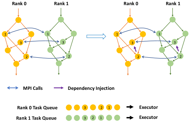
Figure 9: Ensuring the correctness of multi-threaded MPI programs using dependency injection. We make Operator 3 explicitly depend on Operator 2. The bottom shows the working queues for each MPI processor, the MPI operators are serialized in the same order.

To resolve the data race issue, we can explicitly make Operator 3 depend on Operator 2. In this way, we can ensure that the MPI calls Operator 1, 2, and 3 are executed in order. Note this technique sacrifices some concurrency (Operator 2 and Operator 3 cannot be executed concurrently), but the concurrency of most non-MPI operators is still preserved.

4 Benchmarks

The purpose of this section is to present the distributed computing capability of ADCME via MPI. With the MPI operators, ADCME is well suited to parallel applications on clusters with very large numbers of cores. We benchmark individual operators as well as the gradient calculation as a whole. Particularly, we use two metrics for measuring the scaling of the implementation:

1. Weak scaling, i.e., how the solution time varies with the number of processors for a fixed problem size per processor.

2. Strong scaling, i.e., the speedup for a fixed problem size with respect to the number of processors, and is governed by Amdahl’s law.

For most operators, ADCME is just a wrapper of existing third-party parallel computing software (e.g., Hypre). However, for gradient back-propagation, some functions may be missing and are implemented anew. For example, in Hypre, distributed sparse matrices split into multiple stripes, where each MPI rank owns a stripe with continuous row indices. In gradient back-propagation, the transpose of the original matrix is usually needed and such functionalities are missing in Hyper.

Note that ADCME uses hybrid parallel computing models, i.e., a mixture of multithreading programs and MPI communication; therefore, when we talk about one MPI processor, it may contain multiple CPU cores. The MPI processors may also be distributed in different CPUs/nodes, which are interconnected via network communications.

All the experiments are conducted on a cluster with 133 computational node, and each node has 32 cores in total (Intel(R) Xeon(R) CPU E5-2670 0 @ 2.60GHz, 32 GB RAM). The MPI programs are verified with serial programs.

4.1 Transposition

This example benchmarks transposition of a distributed sparse matrix. The transposition operation is very important for gradient back-propagation. We consider solving the Poisson’s equation in $[0,1]^{2}$

$$\nabla\cdot(\kappa(\mathbf{x})\nabla u(\mathbf{x})) =f(\mathbf{x}) \mathbf{x}\in\Omega$$ (7)

$$u(\mathbf{x}) =0 \mathbf{x}\in\partial\Omega$$

Here $f(\mathbf{x})\equiv 1$, and $\kappa(\mathbf{x})$ is approximated by a deep neural network

$$\kappa(\mathbf{x})=\mathcal{N}_{\theta}(\mathbf{x})$$

where $\theta$ is the neural network weights and biases. The equation is discretized using finite difference method on a uniform grid and the discretization leads to a linear system

$$\mathbf{A}\mathbf{u}=\mathbf{f}$$

Here $\mathbf{u}$ is the solution vector and $\mathbf{f}$ is the source vector. Note that $\mathbf{A}$ is a sparse matrix and its entries depend on $\theta$.

The domain is split into multiple patches and each patch correspond to a strip of rows in $\mathbf{A}$. The results are shown in Figure 10. In the plots, we show the strong scaling for a fixed matrix size of 25,000,000$\times$25,000,000 as well as the weak scaling, where each MPI processor owns a patch of the whole mesh and has a size $300\times 300$, i.e., $300^{2}=90000$ rows. The run time for a fixed problem size is effectively reduced as we increase the number of processors, and no stagnation is observed for the current setting. For the weak scaling results, we see only 2$\sim$3 times increase in runtime when we scale up to hundreds of processors.

Figure 10: Strong (left) and weak (right) scaling for transposition of distributed sparse matrix.

4.2 Poisson’s Equation

This example demonstrates the capability of ADCME to use Hypre for solving linear systems in parallel. We show that the overhead of ADCME is quite small compared to the linear solver time. We use the same problem setting as Section 4.1. We formulate the loss function using the numerical solution

$$J(\theta):=\sum_{i\in\mathcal{I}}\left(u(\mathbf{x}_{i})-u_{i}\right)^{2}$$

Here $\mathcal{I}$ consists of 80% randomly picked degrees of freedom for each patch. Figure 11 shows the computational model for solving the Poisson’s equation.

Figure 11: Parallel computing model for solving the Poisson’s equation.

In the strong scaling experiments, we consider a fixed problem size $1800\times 1800$ (mesh size, which implies the matrix size is around 32 million $\times$ 32 million). In the weak scaling experiments, each MPI processor owns a $300\times 300$ block. For example, a problem with 3600 processors has the problem size $90000\times 3600\approx 0.3$ billion.

Figure 12: Runtime for forward computation and gradient back-propagation. Left: each MPI processor has 1 core; right: each MPI processor has 4 cores. We see a jump near 64 cores because this is where network communications start taking place (recall each of our CPUs has 32 cores, and each node has two CPUs). The plots show results of weak scaling, each MPI processor solves a local problem of the same size

We first consider the weak scaling. Figure 12 shows the runtime for forward computation as well as gradient back-propagation. There are two important observations:

1. By using more cores per processor, the runtime is reduced significantly. For example, the runtime for the backward is reduced to around 10 seconds from 30 seconds by switching from 1 core to 4 cores per processor.

2. The runtime for the backward is typically less than twice the forward computation. Although the backward requires solve two linear systems (one of them is in the forward computation), the AMG (algebraic multigrid) linear solver in the back-propagation may converge faster, and therefore costs less than the forward.

Additionally, we show the overhead in Figure 13, which is defined as the difference between total runtime and Hypre linear solver time, of both the forward and backward calculation.

Figure 13: Runtime for forward computation and gradient back-propagation. The plots show results of weak scaling, each MPI processor solves a local problem of the same size. However, each MPI processor may have 1 or 4 cores.

We see that the overhead is quite small compared to the total time, especially when the problem size is large. This indicates that the ADCME MPI implementation is very effective.

Now we consider the strong scaling. In this case, we fixed the whole problem size and split the mesh onto different MPI processors. Figure 14 shows the runtime for the forward computation and the gradient back-propagation. We can reduce the runtime by more than 20 times for the expensive gradient back-propagation by utilizing more than 100 MPI processors. Figure 15 shows the speedup and efficiency. We can see that the 4 cores have smaller runtime compared to 1 core.

Figure 14: Runtime for forward computation and gradient back-propagation. The plots show results of strong scaling, the whole problem size is fixed and we increase the number of MPI processors (each processor has 1 or 4 cores).

Figure 15: Speedup and efficiency for parallel computing of the Poisson’s equation.

Finally, we apply the distributed L-BFGS optimizer to train the deep neural network. The distributed optimizer is constructed from a serial distributed optimizer using the approach described in Section 3.4. Figure 16 illustrate the results at 400-th iteration with 4 and 9 MPI processors respectively. Each processor owns a $300\times 300$ patch. We can see that the estimated DNN-based $\kappa(\mathbf{x})$ is very similar to the exact $\kappa(\mathbf{x})$. Figure 17 also shows the corresponding loss function profiles.

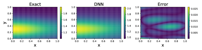
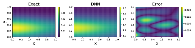
Figure 16: Estimated $\kappa(\mathbf{x})$ at 400-th iteration. The first row shows the result with 4 MPI processors (the mesh size is $600\times 600$), and the second row shows the result with 9 MPI processors (the mesh size is $900\times 900$).

Figure 17: Loss function profiles for distributed optimization with 4 MPI processors (left) and 9 MPI processors (right).

4.3 Acoustic Wave Equation

In this example, we consider the acoustic wave equation with perfectly matched layer (PML) [46, 17]. The governing equation for the acoustic equation is

$$\frac{\partial^{2}u}{\partial t^{2}}=\nabla\cdot(c^{2}\nabla u)$$

where $u$ is the displacement, $f$ is the source term, and $c$ is the spatially varying acoustic velocity. Figure 18 shows the snapshots for the acoustic wave propagation and Figure 19 shows the true velocity model we have used in the acoustic and elastic wave equation examples.

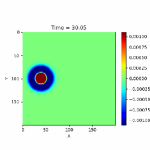
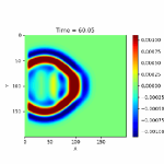
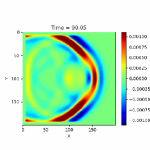
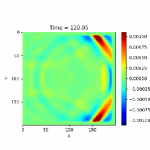
Figure 18: Snapshots of $v_{1}$ for the acoustic wave propagation.

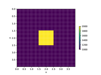
Figure 19: True velocity model $c(\mathbf{x})$.

In the inverse problem, only the wavefield $u$ on the surface is observable, and we want to use this information to estimate $c$. The problem is usually ill-posed, so regularization techniques are usually used to constrain $c$. One approach is to represent $c$ by a deep neural network

$$c(x,y)=\mathcal{N}_{\theta}(x,y)$$

where $\theta$ is the neural network weights and biases. The loss function is formulated by the square loss for the wavefield on the surface. The computational model is shown in Figure 21.

Figure 20: Parallel computing model for solving the acoustic wave equation.

To implement an MPI version of the acoustic wave equation propagator, we use mpi_halo_exchange, which is implemented using MPI and performs the halo exchange mentioned in the last example for both wavefields and axilliary fields. This function communicates the boundary information for each block of the mesh. The following plot shows the computational graph for the numerical simulation of the acoustic wave equation

Figure 21 shows the strong scaling and weak scaling of our implementation. Each processor consists of 32 processors, which are used at the discretion of ADCME’s backend, i.e., TensorFlow. The strong scaling result is obtained by using a $1000\times 1000$ grid and 100 times steps. For the weak scaling result, each MPI processor owns a $100\times 100$ grid, and the total number of steps is 2000. It is remarkable that even though we increase the number of processors from 1 to 100, the total time only increases 2 times in the weak scaling.

Figure 21: Strong and weak scaling of acoustic wave equation.

We also show the speedup and efficiency for the strong scaling case in Figure 22. We can achieve more than 20 times acceleration by using 100 processors (3200 cores in total) and the trend is not slowing down at this scale.

Figure 22: Speedup and efficiency for acoustic wave equations.

4.4 Elastic Wave Equation

In the last example, we consider the elastic wave equation [47]

$$\rho\frac{\partial v_{i}}{\partial t} =\sigma_{ij,j}+\rho f_{i}$$

$$\frac{\partial\sigma_{ij}}{\partial t} =\lambda v_{k,k}+\mu(v_{i,j}+v_{j,i})$$

where $v$ is the velocity, $\sigma$ is the stress tensor, $\rho$ is the density, and $\lambda$ and $\mu$ are the Lamé constants. Similar to the acoustic equation, we use the PML boundary conditions and have observations on the surface. However, the inversion parameters are now spatially varying $\rho$, $\lambda$ and $\mu$. Figure 23 shows snapshots of the wave propagation.

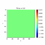
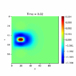
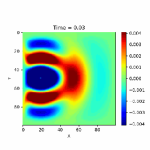
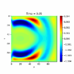
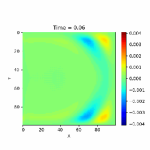
Figure 23: Snapshots of $v_{1}$ for the elastic wave propagation.

As an example, we approximate $\lambda$ by a deep neural network

$$\lambda(x,y)=\mathcal{N}_{\theta}(x,y)$$

and the other two parameters are kept fixed.

We use the same geometry settings as the acoustic wave equation case. Note that elastic wave equation has more state variables as well as auxilliary fields, and thus is more memory demanding. The huge memory cost calls for a distributed framework, especially for large-scale problems.

Additionally, we use fourth-order finite difference scheme for discretizing Equation 2. This scheme requires us to exchange two layers on the boundaries for each block in the mesh. This data communication is implemented using MPI, i.e., mpi_halo_exchange2.

Figure 24 shows the strong and weak scaling. Again, we see that the weak scaling of the implementation is quite effective because the runtime increases mildly even if we increase the number of processors from 1 to 100.

Figure 24: Strong and weak scaling of elastic wave equation.

Figure 25 shows the speedup and efficiency for the strong scaling. We can achieve more than 20 times speedup when using 100 processors.

Figure 25: Speedup and efficiency for elastic wave equations.

5 Conclusion

In this paper we proposed a framework for distributed optimization in scientific machine learning for solving inverse problems. The key is to express numerical simulation using a computational graph. The data communication operations are treated as nodes in the comptuational graph. This view makes the implementation of inverse modeling algorithms quite flexible (modular and testable) and conceptually simple. We also proposed a method to convert existing gradient-based optimization algorithms to MPI-enabled optimizers. These ideas are implemented in the ADCME library, which provides a set of MPI primitives, which can back-propagate gradients. We can also develop customized data communication operators to tailor to specific applications for better performance. To demonstrate the effectiveness of the proposed algorithm, we have trained a neural network that is coupled with either a Poisson’s equation or a wave equation. The PDE is solved numerically and in a distributed way. The results show that our method provides a promising approach towards scalable inverse modeling.

References

References

- [1] Curtis R Vogel. Computational methods for inverse problems. SIAM, 2002.
- [2] Jari Kaipio and Erkki Somersalo. Statistical and computational inverse problems, volume 160. Springer Science & Business Media, 2006.
- [3] Ian Goodfellow, Yoshua Bengio, Aaron Courville, and Yoshua Bengio. Deep learning, volume 1. MIT press Cambridge, 2016.
- [4] Christopher Rackauckas, Yingbo Ma, Julius Martensen, Collin Warner, Kirill Zubov, Rohit Supekar, Dominic Skinner, and Ali Ramadhan. Universal differential equations for scientific machine learning. arXiv preprint arXiv:2001.04385, 2020.
- [5] Kailai Xu, Daniel Z Huang, and Eric Darve. Learning constitutive relations using symmetric positive definite neural networks. arXiv preprint arXiv:2004.00265, 2020.
- [6] Somdatta Goswami, Cosmin Anitescu, Souvik Chakraborty, and Timon Rabczuk. Transfer learning enhanced physics informed neural network for phase-field modeling of fracture. Theoretical and Applied Fracture Mechanics, 106:102447, 2020.
- [7] Maziar Raissi, Paris Perdikaris, and George E Karniadakis. Physics-informed neural networks: A deep learning framework for solving forward and inverse problems involving nonlinear partial differential equations. Journal of Computational Physics, 378:686–707, 2019.
- [8] Xuhui Meng, Zhen Li, Dongkun Zhang, and George Em Karniadakis. Ppinn: Parareal physics-informed neural network for time-dependent pdes. Computer Methods in Applied Mechanics and Engineering, 370:113250, 2020.
- [9] Stephen Boyd, Stephen P Boyd, and Lieven Vandenberghe. Convex optimization. Cambridge university press, 2004.
- [10] David G Luenberger, Yinyu Ye, et al. Linear and nonlinear programming, volume 2. Springer, 1984.
- [11] Adam Paszke, Sam Gross, Soumith Chintala, Gregory Chanan, Edward Yang, Zachary DeVito, Zeming Lin, Alban Desmaison, Luca Antiga, and Adam Lerer. Automatic differentiation in pytorch. 2017.
- [12] Atılım Günes Baydin, Barak A Pearlmutter, Alexey Andreyevich Radul, and Jeffrey Mark Siskind. Automatic differentiation in machine learning: a survey. The Journal of Machine Learning Research, 18(1):5595–5637, 2017.
- [13] Martín Abadi, Paul Barham, Jianmin Chen, Zhifeng Chen, Andy Davis, Jeffrey Dean, Matthieu Devin, Sanjay Ghemawat, Geoffrey Irving, Michael Isard, et al. Tensorflow: A system for large-scale machine learning. In 12th USENIX symposium on operating systems design and implementation (OSDI 16), pages 265–283, 2016.
- [14] R-E Plessix. A review of the adjoint-state method for computing the gradient of a functional with geophysical applications. Geophysical Journal International, 167(2):495–503, 2006.
- [15] Kailai Xu and Eric Darve. Physics constrained learning for data-driven inverse modeling from sparse observations. arXiv preprint arXiv:2002.10521, 2020.
- [16] Daniel Z Huang, Kailai Xu, Charbel Farhat, and Eric Darve. Learning constitutive relations from indirect observations using deep neural networks. Journal of Computational Physics, page 109491, 2020.
- [17] Weiqiang Zhu, Kailai Xu, Eric Darve, and Gregory C Beroza. A general approach to seismic inversion with automatic differentiation. arXiv preprint arXiv:2003.06027, 2020.
- [18] Edgar Gabriel, Graham E Fagg, George Bosilca, Thara Angskun, Jack J Dongarra, Jeffrey M Squyres, Vishal Sahay, Prabhanjan Kambadur, Brian Barrett, Andrew Lumsdaine, et al. Open mpi: Goals, concept, and design of a next generation mpi implementation. In European Parallel Virtual Machine/Message Passing Interface Users’ Group Meeting, pages 97–104. Springer, 2004.
- [19] William Gropp, Rajeev Thakur, and Ewing Lusk. Using MPI-2: advanced features of the message passing interface. MIT press, 1999.
- [20] Mu Wang and Alex Pothen. High order automatic differentiation with mpi. Dep, 3:v0.
- [21] Jean Utke, Laurent Hascoet, Patrick Heimbach, Chris Hill, Paul Hovland, and Uwe Naumann. Toward adjoinable mpi. In 2009 IEEE International Symposium on Parallel & Distributed Processing, pages 1–8. IEEE, 2009.
- [22] Benny N Cheng. A duality between forward adn adjoint mpi communication routines. 2006.
- [23] Michael Griebel and Gerhard Zumbusch. Parallel multigrid in an adaptive pde solver based on hashing and space-filling curves. Parallel Computing, 25(7):827–843, 1999.
- [24] Yvan Notay. An efficient parallel discrete pde solver. Parallel computing, 21(11):1725–1748, 1995.
- [25] Craig C Douglas, Gundolf Haase, and Ulrich Langer. A tutorial on elliptic PDE solvers and their parallelization. SIAM, 2003.
- [26] Ron Bekkerman, Mikhail Bilenko, and John Langford. Scaling up machine learning: Parallel and distributed approaches. Cambridge University Press, 2011.
- [27] Michael I Jordan and Tom M Mitchell. Machine learning: Trends, perspectives, and prospects. Science, 349(6245):255–260, 2015.
- [28] Patrick E Farrell, David A Ham, Simon W Funke, and Marie E Rognes. Automated derivation of the adjoint of high-level transient finite element programs. SIAM Journal on Scientific Computing, 35(4):C369–C393, 2013.
- [29] Sebastian K Mitusch, Simon W Funke, and Jørgen S Dokken. dolfin-adjoint 2018.1: automated adjoints for fenics and firedrake. Journal of Open Source Software, 4(38):1292, 2019.
- [30] Ping He, Charles A Mader, Joaquim RRA Martins, and Kevin J Maki. Dafoam: An open-source adjoint framework for multidisciplinary design optimization with openfoam. AIAA Journal, 58(3):1304–1319, 2020.
- [31] Todd Dupont, Johan Hoffman, Claus Johnson, Robert C Kirby, Mats G Larson, Anders Logg, and L Ridgway Scott. The fenics project. Chalmers Finite Element Centre, Chalmers University of Technology, 2003.
- [32] Hrvoje Jasak, Aleksandar Jemcov, and Zeljko Tukovic. Openfoam: A c++ library for complex physics simulations. 11 2013.
- [33] Tal Ben-Nun and Torsten Hoefler. Demystifying parallel and distributed deep learning: An in-depth concurrency analysis, 2018. cite arxiv:1802.09941.
- [34] Joost Verbraeken, Matthijs Wolting, Jonathan Katzy, Jeroen Kloppenburg, Tim Verbelen, and Jan S Rellermeyer. A survey on distributed machine learning. ACM Computing Surveys (CSUR), 53(2):1–33, 2020.
- [35] Mu Li, David G Andersen, Jun Woo Park, Alexander J Smola, Amr Ahmed, Vanja Josifovski, James Long, Eugene J Shekita, and Bor-Yiing Su. Scaling distributed machine learning with the parameter server. In 11th USENIX Symposium on Operating Systems Design and Implementation (OSDI 14), pages 583–598, 2014.
- [36] Chi-Chung Chen, Chia-Lin Yang, and Hsiang-Yun Cheng. Efficient and robust parallel dnn training through model parallelism on multi-gpu platform. arXiv preprint arXiv:1809.02839, 2018.
- [37] Jeff Bezanson, Alan Edelman, Stefan Karpinski, and Viral B Shah. Julia: A fresh approach to numerical computing. SIAM review, 59(1):65–98, 2017.
- [38] Robert D Falgout and Ulrike Meier Yang. hypre: A library of high performance preconditioners. In International Conference on Computational Science, pages 632–641. Springer, 2002.
- [39] Kailai Xu and Eric Darve. Calibrating multivariate lévy processes with neural networks. In Mathematical and Scientific Machine Learning, pages 207–220. PMLR, 2020.
- [40] Markus Towara, Michel Schanen, and Uwe Naumann. Mpi-parallel discrete adjoint openfoam. In ICCS, pages 19–28, 2015.
- [41] Russell J Hewett and Thomas J Grady II. A linear algebraic approach to model parallelism in deep learning. arXiv preprint arXiv:2006.03108, 2020.
- [42] Dong C Liu and Jorge Nocedal. On the limited memory bfgs method for large scale optimization. Mathematical programming, 45(1-3):503–528, 1989.
- [43] William W Hager and Hongchao Zhang. A survey of nonlinear conjugate gradient methods. Pacific journal of Optimization, 2(1):35–58, 2006.
- [44] Diederik P Kingma and Jimmy Ba. Adam: A method for stochastic optimization. arXiv preprint arXiv:1412.6980, 2014.
- [45] Shigeru Chiba and Rei Ishikawa. Aspect-oriented programming beyond dependency injection. In European Conference on Object-Oriented Programming, pages 121–143. Springer, 2005.
- [46] Marcus J Grote and Imbo Sim. Efficient pml for the wave equation. arXiv preprint arXiv:1001.0319, 2010.
- [47] Dongzhuo Li, Kailai Xu, Jerry M Harris, and Eric Darve. Coupled time-lapse full-waveform inversion for subsurface flow problems using intrusive automatic differentiation. Water Resources Research, 56(8):e2019WR027032, 2020.