Complete and incomplete fusion of ⁷Li projectiles on heavy targets

Abstract

We present a detailed discussion of a recently proposed method to evaluate complete and incomplete fusion cross sections for weakly bound systems. The method is applied to collisions of ⁷Li projectiles on different heavy targets, and the results are compared with the available data. The overall agreement between experiment and theory is fairly good.

I Introduction

Fusion reactions involving weakly bound nuclei have attracted considerable interest over the last few decades Canto et al. (2006); Keeley et al. (2007, 2009); Canto et al. (2015a); Kolata et al. (2016). The low breakup threshold of these nuclei influences fusion in two ways. First, the low binding energy of the clusters within the projectile leads to an extended tail in the nuclear density, which gives rise to a lower Coulomb barrier. This is a static effect that enhances fusion at all collision energies. Second, the couplings with the breakup channel in collisions of these nuclei are very important. They affect elastic scattering and fusion strongly. In addition to the usual direct complete fusion (DCF), where the whole projectile fuses with the target, there is incomplete fusion (ICF), where only a piece of the projectile is capture by the target. Finally, there is the possibility that the projectile breaks up and then all the fragments are absorbed sequentially by the target. This process is known as sequential complete fusion (SCF). The sum of DCF and SCF is called complete fusion (CF), and the sum of all fusion processes is called total fusion (TF).

The DCF and SCF processes cannot be distinguished experimentally. Besides, most experiments measure only the inclusive TF cross section. However, individual CF and ICF cross sections have been measured for some particular projectile-target combinations. There are CF and ICF data available in collisions of ^6,7Li projectiles on ${}^{209}{\rm Bi}$ Dasgupta et al. (2002, 2004), ¹⁵⁹Tb Mukherjee et al. (2006); Broda et al. (1975); Pradhan et al. (2011), ^144,152Sm Rath et al. (2013, 2009, 2012), ¹⁶⁵Ho Thompson et al. (1989), ¹⁹⁸Pt Shrivastava et al. (2013, 2009), ¹⁵⁴Sm Guo et al. (2015), ⁹⁰Zr Kumawat et al. (2012), ¹²⁴Sn Parkar et al. (2018), and ¹⁹⁷Au Palshetkar et al. (2014).

The theoretical determination of individual CF and ICF cross sections has also been a great challenge. Most calculations with this aim are based on classical mechanics Hagino et al. (2004); Dasgupta et al. (2002); Diaz-Torres et al. (2007); Diaz-Torres (2010, 2011), or semiclassical approximations Marta et al. (2014); Kolinger et al. (2018), which do not account properly for important quantum mechanical effects. This shortcoming has been eliminated in a few quantum mechanical models based on the continuum discretized coupled channel method (CDCC). However, in most cases, they can only determine the TF cross section Keeley et al. (2001); Diaz-Torres et al. (2003); Jha et al. (2014); Descouvemont et al. (2015). There is a quantum mechanical method that provides individual CF and ICF cross section Hagino et al. (2000); Diaz-Torres and Thompson (2002), but it can only be applied to collisions where the projectile breaks up into two fragments, with one being much heavier than the other. Recently, Lei and Moro Lei and Moro (2019) determined the CF cross sections for the ^6,7Li + ²⁰⁹Bi systems, extracting it from the total reaction cross section, by subtracting the inelastic, elastic breakup and inclusive nonelastic breakup (NEB) components. The NEB cross section was calculated by the spectator-participant model of Ichimura, Austern, and Vincent Ichimura et al. (1985). Their method is interesting, but it does not allow the calculation of ICF cross sections. There are also the promising quantum mechanical models of Hashimoto et al. Hashimoto et al. (2009) and of Boseli and Diaz-Torres Boselli and Diaz-Torres (2014, 2015), which in their present stage do not allow quantitative calculations of CF and ICF cross sections. In a recent letter Rangel et al. (2020), we proposed a new method using CDCC wave functions. This method has the advantage of being applicable to collisions of any projectile that breaks up into two fragments, independently of their masses. It was used to evaluate CF and ICF cross sections in the ⁷Li + ²⁰⁹Bi collision, and the results were shown to be in excellent agreement with the data of Dasgupta et al. Dasgupta et al. (2002, 2004).

In the present work, we give the details of our method Rangel et al. (2020) and use it to evaluate CF and ICF cross sections in collisions of ⁷Li with several targets. The paper is organized as follows. In section II we introduce our method, expressing the CF, ICF, and TF cross sections in terms of angular momentum-dependent fusion probabilities, which are calculated in appendix A. In section III, we present a detailed discussion of the continuum discretization of ⁷Li, in collisions with a ²⁰⁹Bi target. In section IV, we evaluate CF and ICF cross sections in collisions of ⁷Li projectiles with ²⁰⁹Bi, ¹⁹⁷Au, ¹²⁴Sn, and ¹⁹⁸Pt targets, and compare the predictions of our method with the experimental data. Finally, in section IV we present our conclusions and discuss future extensions of our method.

II Theory of Complete and incomplete fusion

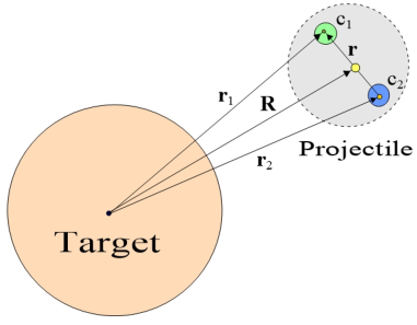
Figure 1: (Color on line) Schematic representation of the projectile, its fragments and the target, and the coordinates involved in the calculations.

In this section we describe the theory to evaluate CF and ICF cross sections introduced in Ref. Rangel et al. (2020), which we use in the present work. We consider the collision of a weakly bound projectile formed by two fragments, $c_{1}$ and $c_{2}$, with a spherical target. The projectile-target relative vector and the vector between the two fragments of the projectile are denoted by ${\bf R}$ and ${\bf r}$, respectively. For simplicity, we do not discuss explicitly spins or orbital angular momenta at this stage. The collision dynamics is dictated by the Hamiltonian

$$\mathbb{H}({\bf R},{\bf r})=h({\bf r})+\hat{K}+\mathbb{U}^{\scriptscriptstyle(1)}(r_{\scriptscriptstyle 1})+\mathbb{U}^{\scriptscriptstyle(2)}(r_{\scriptscriptstyle 2}),$$ (1)

where

$$\mathbb{U}^{\scriptscriptstyle(i)}(r_{\rm\scriptscriptstyle i})\equiv\mathbb{V}^{\scriptscriptstyle(i)}(r_{\scriptscriptstyle i})-i\,\mathbb{W}^{\scriptscriptstyle(i)}(r_{\scriptscriptstyle i})$$ (2)

is the complex interaction between fragment $c_{\scriptscriptstyle i}$ and the target, with $r_{\scriptscriptstyle i}$ representing the distance between their centers. These distances are given by,

$$r_{i}=\left|{\bf R}+{\bf r}^{\prime}_{i}\right|,$$ (3)

where ${\bf r}^{\prime}_{i}$ is the position vector of fragment $c_{i}$ in the reference frame of the projectile. For the situation depicted in Fig. 1, these vectors are

$${\bf r}_{\rm\scriptscriptstyle 1}^{\prime}=\frac{A_{\rm\scriptscriptstyle 2}}{A_{\rm\scriptscriptstyle P}}\,{\bf r}\ \ {\rm and}\ \ {\bf r}_{\rm\scriptscriptstyle 2}^{\prime}=-\frac{A_{\rm\scriptscriptstyle 1}}{A_{\rm\scriptscriptstyle P}}\,{\bf r},$$ (4)

with $A_{i}$ and $A_{\rm\scriptscriptstyle P}$ standing for the mass numbers of fragment $c_{i}$ and the projectile, respectively.

To evaluate the fusion cross sections, we perform CDCC calculations adopting short-range functions for the imaginary potentials $\mathbb{W}^{\rm\scriptscriptstyle(1)}$ and $\mathbb{W}^{\rm\scriptscriptstyle(2)}$. The calculations involve a set of bound channels - subspace B, and a set of continuum-discretized channels (bins) - subspace C. Since the imaginary potentials have short ranges, the total fusion cross section is equal to the absorption cross section, which is given by the well known expression Canto and Hussein (2013)

$$\sigma_{\rm\scriptscriptstyle TF}=\frac{1}{|N|^{2}}\ \frac{K}{E}\ \ \left\langle\ {\rm\Psi}^{\rm\scriptscriptstyle(+)}\,\left|\,{\mathbb{W}}^{(1)}+{\mathbb{W}}^{(2)}\,\right|{\rm\Psi}^{\rm\scriptscriptstyle(+)}\ \right\rangle.$$ (5)

Above, ${\rm\Psi}^{\rm\scriptscriptstyle(+)}$ is the scattering state in a collision with incident wave vector ${\bf K}$ and energy $E$, and $N$ is a normalization constant.

Next, we split the wave function as,

$${\rm\Psi}^{\rm\scriptscriptstyle(+)}({\bf R},{\bf r})={\rm\Psi}^{\rm\scriptscriptstyle B}({\bf R},{\bf r})\ +\ {\rm\Psi}^{\rm\scriptscriptstyle C}({\bf R},{\bf r}),$$ (6)

where ${\rm\Psi}^{\rm\scriptscriptstyle B}$ and ${\rm\Psi}^{\rm\scriptscriptstyle C}$ are respectively its components in the bound and bin subspaces. They are given by the channel expansions

$${\rm\Psi}^{\rm\scriptscriptstyle B}({\bf R},{\bf r}) = \sum_{\beta\,\in\,{\rm\scriptscriptstyle B}}\ \left[\psi_{\beta}({\bf R})\otimes\phi_{\beta}({\bf r})\right]$$ (7)

$${\rm\Psi}^{\rm\scriptscriptstyle C}({\bf R},{\bf r}) = \sum_{\gamma\,\in\,{\rm\scriptscriptstyle C}}\ \left[\psi_{\gamma}({\bf R})\otimes\phi_{\gamma}({\bf r})\right],$$ (8)

where $\phi_{\beta}$ and $\phi_{\gamma}$ are respectively bound and unbound states of the projectile, and $\psi_{\beta}$ and $\psi_{\gamma}$ are the corresponding wave function describing the projectile-target relative motion.

In our method, we assume that matrix-elements of the imaginary potentials connecting bound channels to bins are negligible. Approximations along this line are frequently made in fusion calculations Satchler et al. (1987); Diaz-Torres et al. (2003); Potel et al. (2015). Then, Eq. (5) can be put in the form

$$\sigma_{\rm\scriptscriptstyle TF}=\sigma_{\rm\scriptscriptstyle TF}^{\rm\scriptscriptstyle B}\ +\ \sigma_{\rm\scriptscriptstyle TF}^{\rm\scriptscriptstyle C},$$ (9)

with

$$\sigma_{\rm\scriptscriptstyle TF}^{\rm\scriptscriptstyle B} = \frac{1}{|N|^{2}}\frac{K}{E}\sum_{\beta,\beta^{\prime}\,\in\,{\rm\scriptscriptstyle B}}\ \left\langle\psi_{\beta}\left|W_{\beta\beta^{\prime}}^{\rm\scriptscriptstyle(1)}+W_{\beta\beta^{\prime}}^{\rm\scriptscriptstyle(2)}\,\right|\psi_{\beta^{\prime}}\right\rangle$$ (10)

$$\sigma_{\rm\scriptscriptstyle TF}^{\rm\scriptscriptstyle C} = \frac{1}{|N|^{2}}\frac{K}{E}\sum_{\gamma,\gamma^{\prime}\in\,{\rm\scriptscriptstyle C}}\ \left\langle\psi_{\gamma}\left|W_{\gamma\gamma^{\prime}}^{\rm\scriptscriptstyle(1)}+W_{\gamma\gamma^{\prime}}^{\rm\scriptscriptstyle(2)}\,\right|\psi_{\gamma^{\prime}}\right\rangle.$$ (11)

Above,

$$W_{\alpha\alpha^{\prime}}^{\rm\scriptscriptstyle(i)}=\left(\phi_{\alpha}\left|\mathbb{W}^{\rm\scriptscriptstyle(i)}\right|\phi_{\alpha^{\prime}}\right),$$ (12)

with $\alpha,\alpha^{\prime}$ standing for either $\beta,\beta^{\prime}$ or $\gamma,\gamma^{\prime}$, are the matrix-elements of the imaginary potentials.

Performing angular momentum expansions of the wave functions and the imaginary potentials, the cross sections of Eqs. (10) and (11) can be put in the form

$$\sigma_{\rm\scriptscriptstyle TF}^{\rm\scriptscriptstyle B} = \frac{\pi}{K^{2}}\,\sum_{J}(2J+1)\ \mathcal{P}_{\rm\scriptscriptstyle B}^{\rm\scriptscriptstyle TF}(J)$$ (13)

$$\sigma_{\rm\scriptscriptstyle TF}^{\rm\scriptscriptstyle C} = \frac{\pi}{K^{2}}\,\sum_{J}(2J+1)\ \mathcal{P}_{\rm\scriptscriptstyle C}^{\rm\scriptscriptstyle TF}(J),$$ (14)

with

$$\mathcal{P}_{\rm\scriptscriptstyle B}^{\rm\scriptscriptstyle TF}(J) = \mathcal{P}_{\rm\scriptscriptstyle B}^{\rm\scriptscriptstyle(1)}(J)+\mathcal{P}_{\rm\scriptscriptstyle B}^{\rm\scriptscriptstyle(2)}(J)$$ (15)

$$\mathcal{P}_{\rm\scriptscriptstyle C}^{\rm\scriptscriptstyle TF}(J) = \mathcal{P}_{\rm\scriptscriptstyle C}^{\rm\scriptscriptstyle(1)}(J)+\mathcal{P}_{\rm\scriptscriptstyle C}^{\rm\scriptscriptstyle(2)}(J).$$ (16)

Above, $\mathcal{P}_{\rm\scriptscriptstyle B}^{\sc(i)}(J)$ and $\mathcal{P}_{\rm\scriptscriptstyle C}^{\sc(i)}(J)$ are the probabilities of absorption of fragment $c_{i}$ in bound channels and in the continuum, respectively. They are the contributions of $\mathbb{W}^{\rm\scriptscriptstyle(i)}$ to the TF cross section. A detailed calculation of these quantities is presented in the appendix.

Since $\sigma_{\rm\scriptscriptstyle TF}^{\rm\scriptscriptstyle B}$ is a sum of contributions from bound channels, we assume that the two fragments are absorbed simultaneously. Thus, we write

$$\sigma_{\rm\scriptscriptstyle DCF}=\sigma_{\rm\scriptscriptstyle TF}^{\rm\scriptscriptstyle B}.$$ (17)

The meaning of $\sigma_{\rm\scriptscriptstyle TF}^{\rm\scriptscriptstyle C}$ is not so clear. Since it is a sum of contributions from unbound channels, it must be related to cross sections of the ICF and SCF processes. Thus, the individual cross sections for ICF of fragment $c_{\rm\scriptscriptstyle i}$ (ICFi) and for SCF can be written as

$$\sigma_{\rm\scriptscriptstyle ICFi}=\frac{\pi}{K^{2}}\,\sum_{J}(2J+1)\ \mathcal{P}^{\rm\scriptscriptstyle ICFi}(J)$$ (18)

and

$$\sigma_{\rm\scriptscriptstyle SCF}=\frac{\pi}{K^{2}}\,\sum_{J}(2J+1)\ \mathcal{P}^{\rm\scriptscriptstyle SCF}(J),$$ (19)

where the ICF probabilities, $\mathcal{P}^{\rm\scriptscriptstyle ICFi}(J)$, and the SCF probability, $\mathcal{P}^{\rm\scriptscriptstyle SCF}(J)$, are functions of the absorption probabilities $\mathcal{P}_{\rm\scriptscriptstyle C}^{\rm\scriptscriptstyle(1)}(J)$ and $\mathcal{P}_{\rm\scriptscriptstyle C}^{\rm\scriptscriptstyle(2)}(J)$. These functions will be determined in the next sub-section.

The CF, ICF and TF cross sections are then given by

$$\sigma_{\rm\scriptscriptstyle CF} = \sigma_{\rm\scriptscriptstyle DCF}\,+\,\sigma_{\rm\scriptscriptstyle SCF},$$ (20)

$$\sigma_{\rm\scriptscriptstyle ICF} = \sigma_{\rm\scriptscriptstyle ICF1}\,+\,\sigma_{\rm\scriptscriptstyle ICF2},$$ (21)

$$\sigma_{\rm\scriptscriptstyle TF} = \sigma_{\rm\scriptscriptstyle CF}+\sigma_{\rm\scriptscriptstyle ICF}.$$ (22)

II.1 $J$-dependent elastic, nonelastic and absorption probabilities

We consider a coupled channel problem involving the elastic channel ($\alpha=0$) and $N$ nonelastic channels ($\alpha=1,2,...,N$). The absorption cross section is given in terms of the total reaction cross section and the cross sections for non-elastic channels by the equation

$$\sigma_{\rm abs}=\sigma_{\rm\scriptscriptstyle R}-\sum_{\alpha=1}^{N}\sigma_{\alpha}.$$ (23)

Carrying out angular momentum expansions, we get

$$\sigma_{\rm abs}=\sum_{J=0}^{\infty}\sigma_{\rm abs}(J)=\sum_{J=0}^{\infty}\left[\sigma_{\rm\scriptscriptstyle R}(J)-\sum_{\alpha=1}^{N}\sigma_{\alpha}(J)\right],$$ (24)

with

$$\sigma_{\rm\scriptscriptstyle R}(J) = \frac{\pi}{K^{2}}\ (2J+1)\ \Big{[}1-\left|S_{0}(J)\right|^{2}\Big{]}$$ (25)

$$\sigma_{\alpha}(J) = \frac{\pi}{K^{2}}\ (2J+1)\ \left|S_{\alpha}(J)\right|^{2}.$$ (26)

Then, the $J$-components of the absorption cross section are given by,

$$\sigma_{\rm abs}(J)=A(J)\ \Bigg{[}1\ -\ \sum_{\alpha=0}^{N}\left|S_{\alpha}(J)\right|^{2}\Bigg{]}$$ (27)

where

$$A(J)=2\pi\ \left(\frac{\Lambda}{K}\right)\,\left(\frac{1}{K}\right).$$ (28)

Above, we have introduced the semiclassical angular momentum in $\hbar$ units, $\Lambda=J+1/2$. The two terms within brackets in Eq. (28) correspond respectively to the impact parameter, $b$, and its increment, $\Delta b$, when $\Lambda$ is increased by one unit. Thus, $A(J)$ is the area of a ring with radius $b$ and thickness $\Delta b$. Therefore, $\mathcal{P}_{\alpha}(J)\equiv\left|S_{\alpha}(J)\right|^{2}$ is the probability that the system is in channel-$\alpha$ after a collision with angular momentum $J$. Then, Eq. (27) leads to the relation,

$$\mathcal{P}_{\rm abs}(J)\equiv\frac{\sigma_{\rm abs}(J)}{A(J)}=1\,-\,\sum_{\alpha=0}^{N}\mathcal{P}_{\alpha}(J),$$ (29)

and one gets the normalization relation

$$\mathcal{P}_{\rm abs}(J)+\sum_{\alpha=0}^{N}\mathcal{P}_{\alpha}(J)=1.$$ (30)

II.1.1 Probabities in the CDCC calculation

In our CDCC calculations the target is treated as a heavy inert particle. Then, the $N+1$ channels in the sum of Eq. (30) differ by the state of the projectile. The first term is the elastic channel ($\alpha=0$). The remaining $N$ channels can be split as $N=N_{\rm\scriptscriptstyle B}+N_{\rm\scriptscriptstyle C}$, where $N_{\rm\scriptscriptstyle B}$ is the number of inelastic channels and $N_{\rm\scriptscriptstyle C}$ is the number of bins in the continuum discretization. Then, the sum over the excited states gives the total inelastic probability and the sum over the bin states the elastic breakup probability. That is,

$$\mathcal{P}^{\rm el}(J)=\mathcal{P}_{0}(J),\ \ \ \mathcal{P}^{\rm inel}(J)=\sum_{\alpha=1}^{N_{\rm\scriptscriptstyle B}}\ \mathcal{P}_{\alpha}(J)$$ (31)

and

$$\mathcal{P}^{\rm\scriptscriptstyle EBU}(J)=\sum_{N_{\rm\scriptscriptstyle B}+1}^{N}\ \mathcal{P}_{\alpha}(J).$$ (32)

Since the imaginary potentials in our calculations have short range, absorption represents fusion, of any kind, namely $\mathcal{P}_{\rm abs}(J)=\mathcal{P}^{\rm\scriptscriptstyle TF}(J)$. The normalization condition of Eq. (30) then reads,

$$\mathcal{P}^{\rm\scriptscriptstyle TF}(J)\,+\,\mathcal{P}^{\rm el}(J)\,+\,\mathcal{P}^{\rm inel}(J)\,+\,\mathcal{P}^{\rm\scriptscriptstyle EBU}(J)=1.$$ (33)

The probabilities $\mathcal{P}^{\rm el}$, $\mathcal{P}^{\rm inel}$ and $\mathcal{P}^{\rm\scriptscriptstyle EBU}$ are directly given by the solution of the CDCC equations. The TF probabilites are evaluated by the angular momentum projected version of Eq. (5) (see appendix A).

II.1.2 ICF and SCF Probabities

The contribution from the continuum to the TF probability is

$$\mathcal{P}^{\rm\scriptscriptstyle TF}_{\rm\scriptscriptstyle C}(J)=\mathcal{P}^{\rm\scriptscriptstyle ICF1}(J)\,+\,\mathcal{P}^{\rm\scriptscriptstyle ICF2}(J)\,+\,\mathcal{P}^{\rm\scriptscriptstyle SCF}(J).$$ (34)

However, to evaluate the above probabilities, they must be expresses in terms of absorption probabilities of the two fragments, $\mathcal{P}_{\rm\scriptscriptstyle C}^{\rm\scriptscriptstyle(1)}(J)$ and $\mathcal{P}_{\rm\scriptscriptstyle C}^{\rm\scriptscriptstyle(2)}(J)$, which are calculated in appendix A. Following Refs. Marta et al. (2014); Kolinger et al. (2018); Rangel et al. (2020), we make the intuitive assumptions

$${\mathcal{P}}^{\rm\scriptscriptstyle ICF1}(J) = {\mathcal{P}}^{\rm\scriptscriptstyle(1)}_{\rm\scriptscriptstyle C}(J)\times\left[\ 1-{\mathcal{P}}^{\rm\scriptscriptstyle(2)}_{\rm\scriptscriptstyle C}(J)\ \right]$$ (35)

$${\mathcal{P}}^{\rm\scriptscriptstyle ICF2}(J) = {\mathcal{P}}^{\rm\scriptscriptstyle(2)}_{\rm\scriptscriptstyle C}(J)\times\left[\ 1-{\mathcal{P}}^{\rm\scriptscriptstyle(1)}_{\rm\scriptscriptstyle C}(J)\ \right].$$ (36)

The SCF probability is then obtained inserting Eqs. (16), (35) and (36) into Eq. (34). We get

$${\mathcal{P}}^{\rm\scriptscriptstyle SCF}(J)=2\ {\mathcal{P}}^{\rm\scriptscriptstyle(1)}_{\rm\scriptscriptstyle C}(J)\times{\mathcal{P}}^{\rm\scriptscriptstyle(2)}_{\rm\scriptscriptstyle C}(J).$$ (37)

Note that the factor 2 is essential to satisfy Eq. (16). In fact, it should be expected since differences in the order of events in the sequential absorption of the two fragments must involve different intermediate states.

III Applications

We used our method to study fusion reactions in collisions of ${}^{7}{\rm Li}$ projectiles with ²⁰⁹Bi, ¹⁹⁷Au, ¹²⁴Sn, and ¹⁹⁸Pt targets, for which experimental data are available. In our calculations, ${}^{7}{\rm Li}$ is treated as the two-cluster system: ${}^{7}{\rm Li}\,\equiv\,^{3}{\rm H}+\,^{4}{\rm He}$, with separation energy $B=2.45$ MeV. To determine the cross sections, we used the CF-ICF computer code (unpublished), which evaluates the angular momentum projected version of the expressions of the previous section, derived in the appendix. These expressions involve intrinsic states of the projectile and radial wave functions, which were obtained running the CDCC version of the FRESCO code Thompson (1988).

The real part of the interaction between fragment $c_{i}$ and the target, $\mathbb{V}^{\sc(i)}(r_{i})$, is given by the São Paulo potential Chamon et al. (1997) (SPP), calculated with the densities of the systematic study of Chamon et al. Chamon et al. (2002). The projectile-target potential in the elastic channel is then given by

$$V_{\rm\scriptscriptstyle 00}(R)=\int d^{3}{\bf r}\,\left|\phi_{0}({\bf r})\right|^{2}\ \left[\mathbb{V}^{\sc(1)}(r_{1})\,+\,\mathbb{V}^{\sc(2)}(r_{2})\right],$$ (38)

where $\phi_{0}({\bf r})$ is the ground state wave function of the projectile. Note that this potential takes into account the low breakup threshold of the projectile. This makes its Coulomb barrier lower than the one given by the SPP calculated directly for the projectile-target system. This static effect of the low binding energy enhances the fusion cross section below and above the barrier.

Since the imaginary part of the fragment-target potentials represent fusion absorption, they must be strong and act exclusively in the inner region of the Coulomb barrier. Then, we adopted Woods-Saxon functions with the form,

$$\mathbb{W}^{(i)}(r_{i})=\frac{W_{0}}{1+\exp\left[\left(r_{i}-R_{\rm w}\right)/a_{\rm\scriptscriptstyle w}\right]},\qquad i=1,2,$$ (39)

with the following parameters

$$W_{0}=50\,{\rm MeV},\ \ \ R_{\rm w}=1.0\,\left[A_{i}^{\rm\scriptscriptstyle 1/3}+A_{\rm\scriptscriptstyle T}^{\rm\scriptscriptstyle 1/3}\right]\,{\rm fm};\,\ a_{\rm\scriptscriptstyle w}=0.2\,{\rm fm}.$$ (40)

The intrinsic states of the projectile are solutions of a Schrödinger equation with the Hamiltonian

$$h({\bf r})=K_{\bf r}+V_{\rm\scriptscriptstyle 12}(r_{\rm\scriptscriptstyle 12}),$$ (41)

where $K_{\bf r}$ is the relative kinetic energy of fragments within the projectile, and $V_{\rm\scriptscriptstyle 12}(r_{\rm\scriptscriptstyle 12})$ is the interaction potential between them. The potential used to describe the bound states of the projectile was parametrized by Woods-Saxon functions and derivatives (for the spin-orbit term), with parameters fitted to reproduce its binding energy. Different potentials were used for continuum states. In this case, the parameters were fitted to reproduce the energies and widths of the main resonances. The parameters are basically the ones adopted by Diaz-Torres, Thompson and Beck Diaz-Torres et al. (2003), except for the reduced radius of the central potential. We used $r_{\rm\scriptscriptstyle 0}=1.153$ fm, that gives a slightly better description of the resonances of ⁷Li. Their experimental energies and widths are shown in Table 1, together with the theoretical values obtained in this way.

Table 1: Experimental nnd (2018) and theoretical energies and widths of the ⁷Li resonances. The energies and widths are given in MeV.

$l$	$j^{\pi}$	$\varepsilon^{\rm\scriptscriptstyle th}_{\rm\scriptscriptstyle res}$	$\ \Delta_{\rm th}$	$\varepsilon_{\rm res}^{\rm\scriptscriptstyle exp}$	$\Delta_{\rm\scriptscriptstyle exp}$
3	$7/2^{-}$	2.15	0.1	2.16	0.093
3	$5/2^{-}$	4.54	0.88	4.21	0.88

Multipole expansions of the potentials were carried out, taking into account multipoles up to $\lambda=4$. In the CDCC calculations we used a matching radius of 40 fm and considered total angular momenta up to $J=60\,\hbar$. Note that higher angular momenta, which are essential in calculations of breakup cross sections, do not give relevant contribution to fusion. We checked the convergence of the calculations with respect to these parameters and found that the results are very stable.

III.1 Discretization of the continuum

The channel expansion of Eq. (7) included the ground state of ⁷Li ($j=3/2^{-},l=1$) and its only excited state, with energy $\varepsilon^{*}=0.48$ MeV ($j=1/2^{-},l=1$).

The continuum expansion of Eq. (8) included bins generated by scattering states of the ${}^{3}{\rm H}\,-\,^{4}{\rm He}$ system, with orbital angular momenta $l=0,...,l_{\rm max}$ ($1/2\leq j\leq l_{\rm max}+1/2$) and collision energies from zero to a cut-off energy $\varepsilon_{\rm max}$. The bins were generated by the equation

$$u_{\scriptscriptstyle\beta\,l_{\beta}j_{\beta}}(r)=\int d\varepsilon\ \Gamma_{\rm\scriptscriptstyle\beta}(\varepsilon)\,u_{\scriptscriptstyle\varepsilon l_{\beta}j_{\beta}}(r),$$ (42)

where $u_{\varepsilon l_{\beta}j_{\beta}}(r)$ is the radial wave function in a scattering state with collision energy $\varepsilon$, and angular momentum quantum numbers $l_{\beta},j_{\beta}$, and $\Gamma_{\rm\scriptscriptstyle\beta}(\varepsilon)$ is a weight function concentrated around the energy $\varepsilon_{\rm\scriptscriptstyle\beta}$. In the present work we discretize the continuum in the energy space, using bins with constant values within some interval around $\varepsilon_{\beta}$. Weight functions of this kind, either in the energy or in the momentum space, are commonly used in the literature Sakuragi et al. (1986); Austern et al. (1987); Matsumoto et al. (2003); Thompson and Nunes (2009). The weight functions were given by

$$\Gamma_{\rm\scriptscriptstyle\beta}(\varepsilon) = \frac{1}{\sqrt{\Delta_{\rm\scriptscriptstyle\beta}}},\qquad{\rm if}\ \varepsilon_{\rm\scriptscriptstyle\beta}^{\rm\scriptscriptstyle(+)}\geq\varepsilon_{\rm\scriptscriptstyle\beta}\geq\varepsilon_{\rm\scriptscriptstyle\beta}^{\rm\scriptscriptstyle(-)}$$ (43)

$$= 0,\qquad\qquad\ {\rm otherwise}.$$

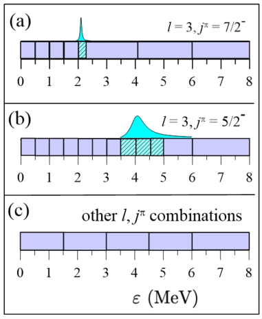
Figure 2: (Color on line) Discretization of the continuum of ⁷Li (panel (a)) and ⁷Li (panel (b)). The narrower bins in the resonances regions are represented in light blue.

Above, $\varepsilon_{\rm\scriptscriptstyle\beta}^{\rm\scriptscriptstyle(\pm)}=\varepsilon_{\rm\scriptscriptstyle\beta}\,\pm\,\Delta_{\rm\scriptscriptstyle\beta}/2$ are the limits of the interval. The bins must cover the whole energy interval from zero to $\varepsilon_{\rm max}$. That is, the upper limit of the $\beta^{\rm th}$ bin, $\varepsilon_{\rm\scriptscriptstyle\beta}\,+\,\Delta_{\rm\scriptscriptstyle\beta}/2$, should coincide with the lower limit of the subsequent bin, $\varepsilon_{\rm\scriptscriptstyle\beta+1}\,-\,\Delta_{\rm\scriptscriptstyle\beta+1}/2$.

The locations and widths of the bins depend on the resonance structure of the projectile. In the absence of resonances, good convergence can be achieved using bins with $\Delta\sim 1-2$ MeV, or even larger than this. To increase the speed of the numerical calculations, the number of bins can be reduced using broader bins as $\varepsilon$ approaches $\varepsilon_{\rm max}$. The situation is more complicated in the presence of sharp resonances. Then, it is necessary to use at least one narrow bin in the resonance region. The meshes for angular momenta with and without resonances are represented in Fig. 2. For $l=3,j^{\pi}=7/2^{\rm\scriptscriptstyle-}$, where there is a sharp resonance at $\varepsilon_{\rm\scriptscriptstyle res}=2.16$ MeV, with $\Delta_{\rm exp}=0.093$ MeV (see Table 1), we used the mesh represented in panel (a). The region below the resonance comprised 4 bins of $\sim 0.5$ MeV, and the resonance was covered by a single bin of width 0.2 MeV. Above the resonance, we used 3 bins of width $\sim 2$ MeV. For $l=3,j^{\pi}=5/2^{\rm\scriptscriptstyle-}$ there is a broader resonance at $\varepsilon_{\rm res}=4.21$ MeV, with $\Delta_{\rm exp}=0.88$ MeV (see Table 1). Then, we adopted the mesh represented in panel (b). Below the resonance, we used 7 bins with $\sim\Delta=0.5$ MeV. The resonance region, between 3.5 and 5 MeV, was covered by 3 bins of about the same width, and the region between 5 and 8 MeV was covered by a bin of 1 MeV and a bin of 2 MeV. Finally in the remaining cases, where there are no resonances, the continuum was discretized with 4 bins of $\Delta=1.5$ MeV and one bin of $\Delta=2.0$ MeV, as shown in panel (c).

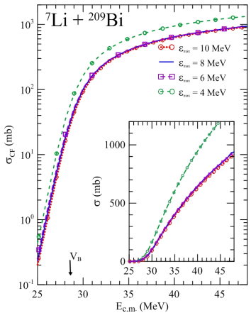
Figure 3: (Color on line) Convergence of $\sigma_{\rm\scriptscriptstyle CF}$ with respect to $\varepsilon_{\rm max}$.

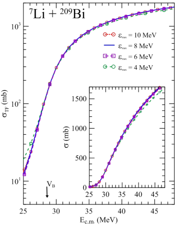
Figure 4: (Color on line) Convergence of $\sigma_{\rm\scriptscriptstyle TF}$ with respect to $\varepsilon_{\rm\scriptscriptstyle max}$.

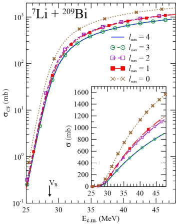
Figure 5: (Color on line) Convergence of $\sigma_{\rm\scriptscriptstyle CF}$ with respect to $l_{\rm\scriptscriptstyle max}$.

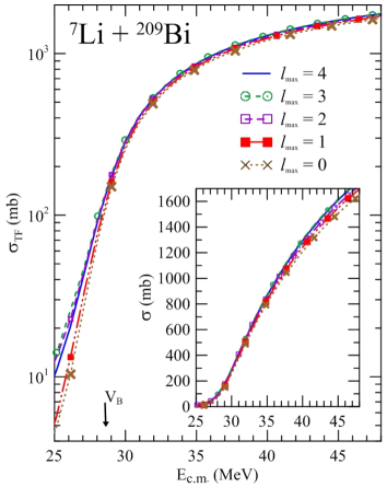
Figure 6: (Color on line) Convergence of $\sigma_{\rm\scriptscriptstyle TF}$ with respect to $l_{\rm\scriptscriptstyle max}$.

We got very good convergence in our calculations using $\varepsilon_{\rm max}=8$ MeV and $l_{\rm max}=3\,\hbar$. This is illustrated in Figs. 3 to 6, which show cross sections of the ${}^{7}{\rm Li}\,+\,^{209}{\rm Bi}$ system, for different values of $\varepsilon_{\rm max}$ and $l_{\rm max}$. The main body of the figures shows cross sections in logarithmic scales, whereas the insets show results in linear scales. In this way, the convergence below and above the barrier can be easily assessed. Inspecting Fig. 3, one concludes that the convergence of $\sigma_{\rm\scriptscriptstyle CF}$ for $\varepsilon_{\rm max}=8$ MeV is excellent. The cross section can hardly be distinguished from the one obtained with the higher cut-off value of $\varepsilon_{\rm max}=10$ MeV. Even for $\varepsilon_{\rm\scriptscriptstyle max}=6$ MeV, the convergence is already quite good. The situation for $\sigma_{\rm\scriptscriptstyle TF}$, shown in Fig. 4, is similar, with the convergence above the barrier being still better. The convergence of the CF and TF cross sections with respect to $l_{\rm max}$, illustrated respectively in Figs. 5 and 6, is also very good. In both cases, the results obtained with $l_{\rm max}=3\,\hbar$ can hardly be distinguished from those obtained with $l_{\rm max}=4\,\hbar$.

Although the above discussion has been restricted to the ${}^{7}{\rm Li}\,+\,^{209}{\rm Bi}$ system, similar behaviors were found for the other system considered in the present work. In all cases we got good convergence with the same discretization of the continuum.

We remark that the convergence study presented above involves the usual parameters of the CDCC method, $\varepsilon_{\rm max}$ and $l_{\rm max}$, which define the truncation of the continuum space. There are, however, internal parameters of FRESCO, related to numerical procedures adopted within the code. Typical applications of FRESCO are calculations of direct reaction cross sections, which depend exclusively on the components of the S-matrix, given by the asymptotic form of the radial wave functions. In such cases, it is not necessary to change the default values of the internal parameters of the code. The situation is more complex in the present work. As shown in appendix A, the CF and ICF cross sections of our method are expressed in terms of radial integrals of the short-range imaginary potentials, multiplied by radial wave functions. Since the main contributions to these integrals come from small radial distances, the asymptotic convergence of the radial wave functions is not enough. One has to make sure that the radial wave functions are stable in the inner region of the barrier, where they are very small. For this purpose, it may be necessary to modify the default value of these parameters.

III.2 Spectroscopic amplitudes

In the calculation of matrix-elements between bound channels and continuum-discretized states, the latter have the ${}^{3}{\rm H}\,-\,^{4}{\rm He}$ cluster configuration intrinsically, and so does the interaction $\mathbb{V}^{\rm\scriptscriptstyle(1)}+\mathbb{V}^{\rm\scriptscriptstyle(2)}$. However, the bound states of ⁷Li do not. Although the amplitude for this configuration is expected to be dominant, it is definitely not equal to one. This statement is supported by the large cross sections for transfer reactions of a single nucleon, observed in collisions of this nucleus Rafiei et al. (2010); Luong et al. (2011, 2013); Zhang et al. (2018). The probabilities of finding the dominant cluster configuration in ^6,7Li is expected to be of the order of 70% Watanabe et al. (2015). Then, the bound-continuum matrix elements should be multiplied by some spectroscopic amplitude, $\mathcal{S}$, say in the $\{0.7-1.0\}$ range. This amplitude could be neglected in qualitative calculations, but not if one aims at a quantitative description of the data.

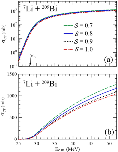
Figure 7: (Color on line) CF cross sections calculated with different values of the spectroscopic amplitude.

Since the inclusion of the spectroscopic amplitude weakens the couplings with the breakup channel, it is expected to enhance the DCF cross section and suppress ICF. The former effect is illustrated in Fig. 7, that shows CF cross sections calculated with the spectroscopic amplitudes: $\mathcal{S}=0.7,0.8,0.9$ and 1.0. The results are show in logarithmic (panel (a)) and linear scales (panel (b)). In the logarithmic plot, the curves for the different spectroscopic amplitudes can hardly be distinguished. However, the influence of $\mathcal{S}$ can be observed in the linear plot. For variations of $\mathcal{S}$ in the $\{0.7,1.0\}$ range, the cross section changes up to $\sim 20\%$. Unfortunately, there are no accurate calculations of the spectroscopic amplitude. Then, we treat it as a free parameter, that can vary between 0.7 and 1.0.

Deviations of the bound states of the projectile from the ${}^{3}{\rm H}\,-\,^{4}{\rm He}$ cluster configuration may also affect diagonal matrix elements of the interaction. They are expected to modify the barrier of the $V_{\rm\scriptscriptstyle 00}(R)$ potential. However, such effects are not expected to be very important. This potential is basically determined by the densities of the collision partners, and it is very sensitive to the long tail of the projectile’s density. This has been taken into account, through the use of a $V_{12}$ potential that reproduces the experimental binding energy of ⁷Li. Although a more careful study of this problem is called for, we will leave it to a future work.

III.3 Complete fusion cross sections

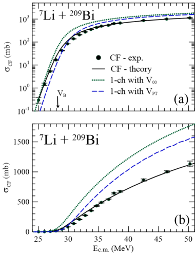
Figure 8: (Color on line) Calculated CF cross sections for the ⁷Li + ²⁰⁹Bi system (solid black line) in comparison with the data of Refs. Dasgupta et al. (2002, 2004) (open circles).

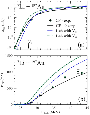
Figure 9: (Color on line) Same as Fig. 8, but for the ⁷Li + ¹⁹⁷Au system. Here the data are from Refs. Palshetkar et al. (2014); nnd (2018).

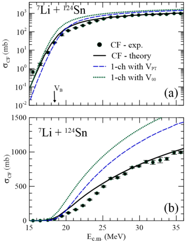
Figure 10: (Color on line) Same as Fig. 8 but now the system is ⁷Li + ¹²⁴Sn. Here, the system is ⁷Li + ¹²⁴Sn and the data are from Ref. Parkar et al. (2018).

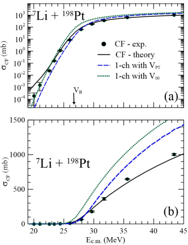
Figure 11: (Color on line) Same as Fig. 8, but for the ⁷Li + ¹⁹⁸Pt system. Here the data are from Ref. Shrivastava et al. (2013).

We used our theory to calculate CF cross sections for collisions of ⁷Li projectiles with ²⁰⁹Bi, ¹⁹⁷Au, ¹²⁴Sn, and ¹⁹⁸Pt targets. These targets have the advantage of not having excited states strongly coupled to the elastic channel. The results (solid black lines) are shown in Figs. 8 to 11. In each case, they are compared with the available experimental data. All calculations were performed with the spectroscopic amplitude $\mathcal{S}=0.8$, which gave best results for the ⁷Li + ²⁰⁹Bi system. Note that the present results for this system are very close to the ones presented in our previous work Rangel et al. (2020), but they are not exactly the same. This is due to the inclusion of the spectroscopic amplitude and to the use of a slightly improved mesh in the continuum discretization.

Figs. 8 to 11 also show cross sections of two one-channel calculations. In the first (green dotted lines), we used the nuclear potential $V_{\rm\scriptscriptstyle 00}(R)$, which is obtained by folding the fragments-target interactions with the ground state density of the projectile (see Eq. (38)). In the second (blue dashed lines), we used the São Paulo potential between the projectile and the target, which ignores the cluster structure of ⁷Li completely. Thus, the former takes into account the static effect of the low breakup threshold, whereas the latter does not. Both one-channel calculations were performed with typical short-range imaginary potentials, $W_{\rm\scriptscriptstyle PT}(R)$, given by WS functions with radii $R_{0}=1.0\,\left(A_{\rm\scriptscriptstyle P}^{\rm\scriptscriptstyle 1/3}\,+\,A_{\rm\scriptscriptstyle T}^{\rm\scriptscriptstyle 1/3}\right)$ fm, depth $W_{0}=100$ MeV and diffusivity $a=0.2$ fm.

The overall agreement between the CF cross sections calculated by our method and the experimental data is quite good. The theoretical cross sections for the ${}^{7}{\rm Li}+^{209}$Bi (Fig. 8), ${}^{7}{\rm Li}+^{197}$Au (Fig. 9), and ${}^{7}{\rm Li}+^{124}$Sn (Fig. 10) systems are very close to the data at all collision energies, above and below the Coulomb barrier. In the case of the ¹⁹⁸Pt target (Fig. 11), the situation is not as good. The theoretical CF cross section is in excellent agreement with the data around and above the Coulomb barrier, but it overestimates the experimental results at energies well below $V_{\rm\scriptscriptstyle B}$. In fact, this problem is not related to the target. It is a consequence of the extended energy range of the experiment Shrivastava et al. (2013). It reaches energies $\sim 6$ MeV below the Coulomb barrier, where the cross sections are as low as $\sim 10^{-4}$ mb. The data for the other systems studied here are restricted to energies $E_{\rm c.m.}\gtrsim V_{\rm\scriptscriptstyle B}-4\,{\rm MeV}$, where the cross sections are three orders of magnitude larger.

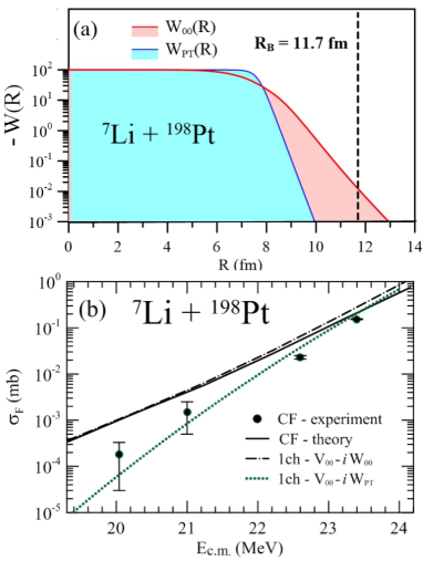
Figure 12: (Color on line) (a) The imaginary potentials $W_{\rm\scriptscriptstyle 00}(R)$ and $W_{\rm\scriptscriptstyle PT}(R)$, shown in a logarithmic scale; (b) Fusion cross sections at very low energies. The CF cross section of our method (solid green line), and the fusion cross sections of one-channel calculations with the potentials $V_{\rm\scriptscriptstyle 00}(R)-iW_{\rm\scriptscriptstyle PT}(R)$ (red dotted line) and $V_{\rm\scriptscriptstyle 00}(R)-iW_{\rm\scriptscriptstyle 00}(R)$ (black dot-dashed line) are compared with the CF data of Refs. Shrivastava et al. (2013). See the text for details.

The inaccuracy of the theoretical CF cross section at energies well below $V_{\rm\scriptscriptstyle B}$ can be traced back to the imaginary potential, $W_{\rm\scriptscriptstyle 00}(R)$, used in the CDCC calculations. This potencial, evaluated internally within the FRESCO code, is given by the expression

$$W_{\rm\scriptscriptstyle 00}(R)=\int d^{3}{\bf r}\,\left|\phi_{0}({\bf r})\right|^{2}\ \left[\mathbb{W}^{\sc(1)}(r_{1})\,+\,\mathbb{W}^{\sc(2)}(r_{2})\right],$$ (44)

where $r_{1}$ and $r_{2}$ are the distances between the centres of the two fragments and the target. Although the ranges of the imaginary potentials $\mathbb{W}^{\sc(i)}$ are very short, the long tail of $\left|\phi_{0}({\bf r})\right|^{2}$ extends $W_{\rm\scriptscriptstyle 00}(R)$ to large distances, beyond $R_{\rm\scriptscriptstyle B}$. This is illustrated in panel (a) of Fig. 12, which compares the imaginary potentials $W_{\rm\scriptscriptstyle 00}(R)$ and $W_{\rm\scriptscriptstyle PT}(R)$. Clearly, the tail of $W_{\rm\scriptscriptstyle 00}(R)$ has a considerably longer range. This difference is not relevant at collision energies above $V_{\rm\scriptscriptstyle B}$, where the incident wave reaches the inner region of the barrier, where the two imaginary potentials are very strong. In this case, the wave is strongly absorbed by both imaginary potentials. In this way, the fusion cross sections calculated with $W_{\rm\scriptscriptstyle 00}(R)$ and $W_{\rm\scriptscriptstyle PT}(R)$ are very close. The situation is different at very low collision energies, where the transmission coefficient through the barrier is extremely small. Then, the cross section has a strong dependence on the tail of the imaginary potential, which, as shown in the figure, is much longer for $W_{\rm\scriptscriptstyle 00}(R)$. However, this long-range absorption cannot be associated with fusion. Since the relevant direct channel, namely breakup, is explicitly included in the CDCC equations, this kind of absorption is spurious. It has no physical meaning.

A more quantitative picture of the problem is presented in panel (b) of Fig. 12, which shows the data of Refs. Dasgupta et al. (2002, 2004) at energies well below the Coulomb barrier, in comparison with different theoretical cross sections. The black solid line and the green dotted line are the same curves of Fig. 11. They represent, respectively, the CF cross section calculated by our method, and the one-channel cross section obtained with the complex potential $U=V_{\rm\scriptscriptstyle 00}-i\,W_{\rm\scriptscriptstyle PT}$. The third curve (black dot-dashed line) represents the results of a one-channel calculation with the potential $U=V_{\rm\scriptscriptstyle 00}-i\,W_{\rm\scriptscriptstyle 00}$. It corresponds to the limit of our CDCC calculation when all channel-couplings are switched off. The difference between the two one-channel calculations is the range of the imaginary potential. First, one notices that the CF cross section converges to the black dot-dashed line at very low energies. This is not surprising, since the coupling matrix-elements become negligibly small in the low energy limit. On the other hand, at the lowest energies, these cross sections become much larger than the one calculated with $W_{\rm\scriptscriptstyle PT}$, which is in very good agreement with the data. Therefore, one concludes that the inaccuracy of our CF cross section at energies well below $V_{\rm\scriptscriptstyle B}$ arises from the spurious tail of the imaginary potential in the CDCC calculations. In principle, this shortcoming could be easily fixed by correcting the asymptotic behavior of $W_{\rm\scriptscriptstyle 00}(R)$. However, this is not an easy task, since it would require internal modifications of the FRESCO code.

III.3.1 The static effect of the low breakup threshold

As mentioned before, the low breakup threshold of ⁷Li affects the CF cross section in two ways. The first is a static effect, arising from the low energy binding the triton to the $\alpha$-particle, which leads to a long tail in the nuclear density. This makes the Coulomb barrier lower, enhancing fusion. On the other hand, the reaction dynamic is strongly affected by couplings with the breakup channel. This has a major influence on fusion, as will be demonstrated in the next sub-section.

Table 2: Coulomb barriers of $V_{\rm\scriptscriptstyle PT}$ and $V_{\rm\scriptscriptstyle 00}$, for the systems studied in this work. The fourth column gives the barrier lowering in each case, and the fifth column is the ratio of the one-channel fusion cross sections calculated with the potentials $V_{\rm\scriptscriptstyle 00}$ and $V_{\rm\scriptscriptstyle PT}$, at 10 MeV above $V^{\rm\scriptscriptstyle 00}_{\rm\scriptscriptstyle B}$. See the text for details.

System	$Z_{\rm\scriptscriptstyle T}$	$V^{\rm\scriptscriptstyle PT}_{\rm\scriptscriptstyle B}$	$V^{\rm\scriptscriptstyle 00}_{\rm\scriptscriptstyle B}$	$\Delta V_{\rm\scriptscriptstyle B}$	$\mathcal{R}^{\rm\scriptscriptstyle 00}_{\rm\scriptscriptstyle PT}$
7Li + 209Bi	83	29.36	28.29	1.07	1.21
7Li + 197Au	79	28.25	27.21	1.04	1.20
7Li + 198Pt	78	27.83	26.81	1.02	1.21
7Li + 124Sn	50	19.29	18.50	0.79	1.18

Table 2 shows Coulomb barriers associated with $V_{\rm\scriptscriptstyle PT}$ and $V_{\rm\scriptscriptstyle 00}$, denoted respectively by $V^{\rm\scriptscriptstyle PT}_{\rm\scriptscriptstyle B}$ and $V^{\rm\scriptscriptstyle 00}_{\rm\scriptscriptstyle B}$. As expected, the latter is systematically lower than the former. The reduction of the barrier height increases with the charge of the target (or with the barrier height). For the systems studied in this work, it ranges from $\sim 0.8$ to $\sim 1.1$ MeV. The barrier lowering enhances the fusion cross section for the potential $V_{\rm\scriptscriptstyle 00}$, with respect to that for $V_{\rm\scriptscriptstyle PT}$. At $\sim 10$ MeV above the barrier, the ratio of the two cross sections for the four systems is of the order of 1.2 or, more precisely, between 1.18 and 1.21.

III.3.2 CF suppressions at above-barrier energies

Now we compare the suppressions of CF for the different systems studied here. Since the cross sections depend on trivial factors, like the charges and sizes of the collision partners, direct comparisons of $\sigma_{\rm\scriptscriptstyle CF}$ do not give reliable information on reaction mechanisms. For a proper comparison, one should first eliminate the influence of such undesirable factors. This is done through transformations on the cross sections and collision energies, known as reduction procedures. Several proposals can be found in the literature Canto et al. (2015b), but the most effective procedure for fusion data is the so called fusion function method Canto et al. (2009a, b). It consists in the following transformations:

$$\ E\ \longrightarrow\ x=\frac{E-V_{\rm\scriptscriptstyle B}}{\hbar\omega},\qquad\sigma_{\rm\scriptscriptstyle F}\ \longrightarrow\ F(x)=\frac{2E}{R_{\rm\scriptscriptstyle B}^{2}\hbar\omega}\times\sigma_{\rm\scriptscriptstyle F}.$$ (45)

This method is based on the Wong’s approximation Wong (1973) for the fusion cross section,

$$\ \sigma_{\rm\scriptscriptstyle F}^{\rm\scriptscriptstyle W}=R_{\rm\scriptscriptstyle B}^{2}\ \frac{\hbar\omega}{2E}\,\ln\left[1+\exp\left(2\pi\ \frac{E-V_{\rm\scriptscriptstyle B}}{\hbar\omega}\right)\right].$$ (46)

It can be immediately checked that if the fusion cross section is well approximated by Wong’s formula, the fusion function takes the universal form

$$\ F_{0}(x)=\Big{[}1+\exp\left(2\pi\,x\right)\Big{]}.$$ (47)

This expression was called the Universal Fusion Function (UFF) in Refs. Canto et al. (2009a, b). Deviations from this behaviour are then associated with particular nuclear structure properties of the collision partners.

To carry out a comparative study of CF suppression at above-barrier energies, we apply the above prescription to collisions of ⁷Li with the ²⁰⁹Bi, ¹⁹⁷Au, ¹²⁴Sn, and ¹⁹⁸Pt targets. We consider both the theoretical and experimental CF cross sections, discussed in the previous sub-sections. The results are denoted by $F_{\rm th}(x)$ and $F_{\rm exp}(x)$, respectively. Further, there are two possibilities. The transformations of Eq. (45) can be based on the barrier parameters of the potential $V_{\rm\scriptscriptstyle 00}$ ($V_{\rm\scriptscriptstyle B}^{\rm\scriptscriptstyle 00},R_{\rm\scriptscriptstyle B}^{\rm\scriptscriptstyle 00}$ and $\hbar\omega^{\rm\scriptscriptstyle 00}$), or on the parameters of $V_{\rm\scriptscriptstyle PT}$ ($V_{\rm\scriptscriptstyle B}^{\rm\scriptscriptstyle PT},R_{\rm\scriptscriptstyle B}^{\rm\scriptscriptstyle PT}$ and $\hbar\omega^{\rm\scriptscriptstyle PT}$). In this way, one can evaluate two theoretical fusion functions, $F_{\rm th}^{\rm\scriptscriptstyle 00}(x)$ and $F_{\rm th}^{\rm\scriptscriptstyle PT}(x)$, and two experimental fusion functions, $F_{\rm exp}^{\rm\scriptscriptstyle 00}(x)$ and $F_{\rm exp}^{\rm\scriptscriptstyle PT}(x)$. Note that the fusion functions $F^{\rm\scriptscriptstyle 00}(x)$ and $F^{\rm\scriptscriptstyle PT}(x)$ have very different meanings, as discussed below.

In the present work, the investigated nuclear structure property is the low breakup threshold of ⁷Li. Since we chose targets that do not have excited states strongly coupled to the elastic channel, the CF fusion functions may be directly compared with the UFF. As the potential $V_{\rm\scriptscriptstyle PT}$ completely ignores the cluster structure of the projectile and its binding energy, comparisons of $F_{\rm th}^{\rm\scriptscriptstyle PT}(x)$ and of $F_{\rm exp}^{\rm\scriptscriptstyle PT}(x)$ with the UFF give the global influence of the low binding on the theoretical and on the experimental CF cross sections, respectively. That is, they measure the net result of the competition between the barrier lowering enhancement and breakup coupling suppression on CF. On the other hand, comparisons of $F_{\rm th}^{\rm\scriptscriptstyle 00}$ and $F_{\rm exp}^{\rm\scriptscriptstyle 00}$ with the UFF give a different piece of information. Since $V_{\rm\scriptscriptstyle 00}$ takes into account the long tail of the ⁷Li density, the static effects associated with the barrier lowering are cancelled in these fusion functions. Therefore, their comparisons with the UFF measure exclusively the influence of couplings with the breakup channel.

Fig. 13 shows the theoretical fusion functions for the systems studied here. Since we are interested in the suppression at above-barrier energies, the plots are shown only in a linear scale. First, one notices that both the $F_{\rm th}^{\rm\scriptscriptstyle 00}$ and $F_{\rm th}^{\rm\scriptscriptstyle PT}$ fusion functions are nearly system independent. The lines for the different targets can hardly be distinguished from each other. To very good approximations, one can write:

$$F_{\rm th}^{\rm\scriptscriptstyle 00}(x)\simeq 0.67\times F_{0}(x);\ \ \ F_{\rm th}^{\rm\scriptscriptstyle PT}(x)\simeq 0.58\times F_{0}(x),$$ (48)

where $F_{0}(x)$ is the universal fusion function of Eq. (47).

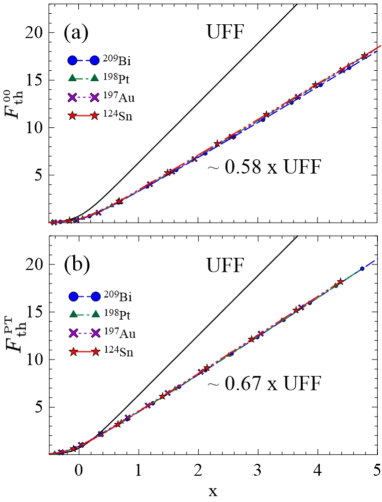
Figure 13: (Color on line) Theoretical fusion functions $F_{\rm th}^{\rm\scriptscriptstyle 00}$ (panel (a)) and $F_{\rm th}^{\rm\scriptscriptstyle PT}$ (panel (b)) in collisions of ⁷Li with the ²⁰⁹Bi, ¹⁹⁷Au, ¹²⁴Sn and ¹⁹⁸Pt targets. See the text for details.

The above equation indicates that $F_{\rm th}^{\rm\scriptscriptstyle 00}$ and $F_{\rm th}^{\rm\scriptscriptstyle PT}$ are suppressed with respect to the UFF by 33 and 42%, respectively.

Fig. 14 shows the experimental fusion functions corresponding to the theoretical curves of the previous figure. The dotted lines represent the predictions of our theory for the two fusion functions, within the $0.67\times F_{0}(x)$ and $0.58\times F_{0}(x)$ approximations. Clearly the data follow very closely the behaviour predicted by the theory, except por a few data points that present small fluctuations around the dotted lines.

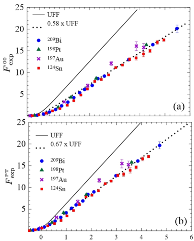
Figure 14: (Color on line) Experimental fusion functions $F_{\rm exp}^{\rm\scriptscriptstyle 00}$ (panel (a)) and $F_{\rm exp}^{\rm\scriptscriptstyle PT}$ (panel (b)) in collisions of ⁷Li with the ²⁰⁹Bi, ¹⁹⁷Au, ¹²⁴Sn and ¹⁹⁸Pt targets. See the text for details.

Usually, CF suppression factors are obtained comparing the data with predictions of barrier penetration models (or results of one-channel calculations), based on projectile-target potentials that ignore the low breakup threshold. Thus, they should be compared with suppression factors extracted from $F_{\rm exp}^{\rm\scriptscriptstyle PT}$. Dasgupta et al. Dasgupta et al. (2002, 2004) studied the ⁷Li + ²⁰⁹Bi system, and found a ratio of 0.74 between the CF data and predictions of barrier penetration models. This is a bit larger than the 0.67 factor, appearing in Fig. 14. The difference can be traced back to the different potential used by these authors in their barrier penetration model calculation. They adopted the Akyüz-Winther (AW) potential, instead of the SPP used in the present work. The barrier for the AW potential is 0.4 MeV higher than that for the SPP Canto et al. (2014) and, consequently, the cross sections obtained with the former is $\sim 10\%$ lower than that of the SPP. Taking this difference into account, our suppression factor becomes very close to theirs.

III.4 Incomplete fusion cross sections

III.4.1 ⁷Li + ²⁰⁹Bi

Fig. 15 shows ICF cross sections for the ${}^{7}{\rm Li}\,+\,^{209}{\rm Bi}$ system calculated by the method of the present work. The cross section for the triton (${\rm ICF}_{t}$) and $\alpha$-particle (${\rm ICF}_{\alpha}$) captures are represented, respectively, by a green dashed line and a blue dotted line. The solid black line corresponds to the full ICF cross section, namely $\sigma_{\rm\scriptscriptstyle ICF}=\sigma_{{\rm\scriptscriptstyle ICF}_{\scriptscriptstyle t}}+\sigma_{\rm\scriptscriptstyle ICF_{\alpha}}$. Our results are compared to the ICF data of Dasgupta et al. Dasgupta et al. (2002, 2004), obtained detecting characteristic $\alpha$-particles. Note that this experiment could not distinguish the ICF_t and the ICF_α components of $\sigma_{\rm\scriptscriptstyle ICF}$. To clarify the situation, we give some details of this work. The ICF_t process leads to the formation of ²¹²Po, and the lighter ^211,210,209Po isotopes, through successive neutron emissions. On the other hand, ICF_α produces ²¹³At and other lighter isotopes by neutron evaporation. In both cases, the Po and the At isotopes de-excite by $\alpha$-decay. The emitted $\alpha$-particles are detected, and the parent nuclei are identified by their energies and half-lives. In principle, this procedure could lead to the individual ICF_t and ICF_α cross section. However, ²¹⁰At decays almost completely by $\beta^{\rm\scriptscriptstyle+}+{\rm EC}$ to ²¹⁰Po. In this way, the At and the Po decay chains are mixed. Thus, an $\alpha$-particle emitted by ²¹⁰Po is a signature of ICF, but one cannot tell whether it is ICF_t or ICF_α. For this reason, this experiment determines only their sum, $\sigma_{\rm\scriptscriptstyle ICF}$.

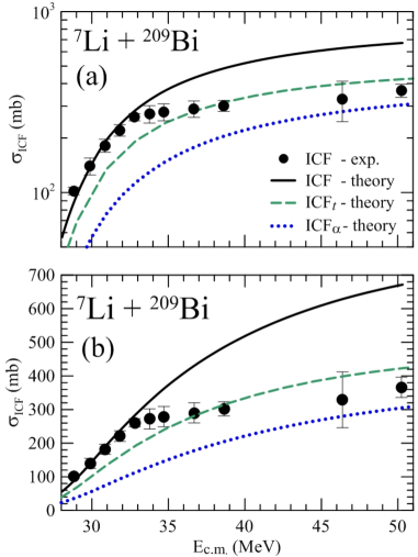
Figure 15: (Color on line) Incomplete fusion cross sections for the ⁷Li + ²⁰⁹Bi system calculated by our method, in comparison with the ICF data of Refs. Dasgupta et al. (2002, 2004).

By inspecting Fig. 15, we find that the predictions of our theory at low energies are very accurate. The four data points at the lowest energies fall on top of the theoretical curve. However, the calculated cross section above $\sim 35$ MeV overestimates the data. It grows continuously with the energy, whereas the data are roughly constant. Nevertheless, the discrepancy between theory and experiment might, at least in part, arise from missing contributions from ²⁰⁹Po, in the decay chains of both ICF processes. Owing to its long half-life ($\sim 100$ y), its $\alpha$-decay could not be measured. Dasgupta et al. Dasgupta et al. (2002, 2004) estimated the contribution from this channel using the PACE evaporation code Gavron (1980). They found that it should be negligible at the lowest energies of the experiment, but it becomes important above $\sim 36$ MeV. For this reason, they suggested that the data above this limit should be considered as a lower bound to the actual cross section. Thus, our results may be consistent with the data in this energy range.

Finally, comparing the theoretical ICF_t and ICF_α cross sections, we conclude that the ICF_t component of $\sigma_{\rm\scriptscriptstyle ICF}$ is dominant, but the ${\rm ICF_{\alpha}}$ component is appreciable. At above barrier energies, $\sigma_{\rm\scriptscriptstyle ICF_{\alpha}}$ is about 50% of $\sigma_{{\rm\scriptscriptstyle ICF}_{\scriptscriptstyle t}}$.

III.4.2 ⁷Li + ¹⁹⁷Au

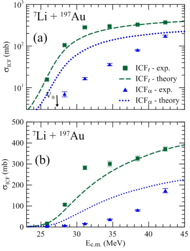
Figure 16: (Color on line) ICF_t and ICF_α cross sections for the ⁷Li + ¹⁹⁷Au system calculated by our method, in comparison to the data of Palshetkar et al. Palshetkar et al. (2014); nnd (2018).

Fig. 16 shows the $\sigma_{{\rm\scriptscriptstyle ICF}_{\scriptscriptstyle t}}$ (green dashed line) and $\sigma_{\rm\scriptscriptstyle ICF_{\alpha}}$ (blue dotted line) cross sections for the ${}^{7}{\rm Li}\,+\,^{197}{\rm Au}$ system, calculated by our method. The results are compared to the experimental cross sections of Palshetkar et al. Palshetkar et al. (2014); nnd (2018), measured by the gamma-ray spectroscopy method (in- and off-beam). Note that in this experiment, it was possible to determine individual cross sections for each ICF process. Inspecting the figure, we conclude that the $\sigma_{{\rm\scriptscriptstyle ICF}_{\scriptscriptstyle t}}$ cross section predicted by our method reproduces very well the data, except for the data point at $E_{\rm c.m.}\simeq 31$ MeV, which is $\sim 30\%$ larger than the theoretical prediction.

On the other hand, the theoretical predictions for $\sigma_{\rm\scriptscriptstyle ICF_{\alpha}}$ are well above the data, except for the data point at the highest energy, where the difference between the two cross sections is small. Note that the $\sigma_{\rm\scriptscriptstyle ICF_{\alpha}}/\sigma_{{\rm\scriptscriptstyle ICF}_{\scriptscriptstyle t}}$ ratio at above-barrier energies predicted by our method is of the order of 50%, similarly to the ⁷Li + ²⁰⁹Bi system. The origin of the discrepancy between our predictions for $\sigma_{\rm\scriptscriptstyle ICF_{\alpha}}$ and the data is not clear to us. It calls for further investigations.

III.4.3 ⁷Li + ¹²⁴Sn

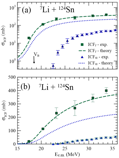
Figure 17: (Color on line) Same as the previous figure, but now the system is ⁷Li + ¹²⁴Sn, and the data are from Parkar et al. Parkar et al. (2018).

Fig. 17 shows $\sigma_{{\rm\scriptscriptstyle ICF}_{\scriptscriptstyle t}}$ and $\sigma_{\rm\scriptscriptstyle ICF_{\alpha}}$ cross sections calculated by our method for the ${}^{7}{\rm Li}\,+\,^{124}{\rm Sn}$ system. The notation of the curves is the same as in the previous figure. Our results are compared to the experimental $\sigma_{{\rm\scriptscriptstyle ICF}_{\scriptscriptstyle t}}$ and $\sigma_{\rm\scriptscriptstyle ICF_{\alpha}}$ cross sections of Parkar et al. Parkar et al. (2018), also measured by the gamma-ray spectroscopy method (in- and off-beam). The situation is very similar to that observed for the previous system. The $\sigma_{{\rm\scriptscriptstyle ICF}_{\scriptscriptstyle t}}$ cross section predicted by our method is in excellent agreement with the data, whereas our predictions for $\sigma_{\rm\scriptscriptstyle ICF_{\alpha}}$ are much larger than the data. At the highest energies of the experiment, the theoretical $\sigma_{\rm\scriptscriptstyle ICF_{\alpha}}/\sigma_{{\rm\scriptscriptstyle ICF}_{\scriptscriptstyle t}}$ ratio is slightly above 50%, while the experimental ratio is of the order of 10%.

III.4.4 ⁷Li + ¹⁹⁸Pt

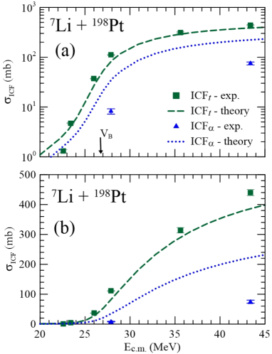
Figure 18: (Color on line) Same as the previous figure, but now the system is ⁷Li + ¹⁹⁴Pt, and the data are from Shrivastava et al.Shrivastava et al. (2013).

Fig. 18 shows $\sigma_{{\rm\scriptscriptstyle ICF}_{\scriptscriptstyle t}}$ and $\sigma_{\rm\scriptscriptstyle ICF_{\alpha}}$ cross sections calculated by our method for the ${}^{7}{\rm Li}\,+\,^{198}{\rm Pt}$ system, in comparison with the data of Shrivastava et al. Shrivastava et al. (2013). Again, the experiment used the gamma-ray spectroscopy method and was able to measure individual cross sections for the two ICF processes. The situation is similar to those observed for the ¹⁹⁷Au and ¹²⁴Sn targets. The theoretical predictions for $\sigma_{{\rm\scriptscriptstyle ICF}_{\scriptscriptstyle t}}$ are very close to the data, whereas those for $\sigma_{\rm\scriptscriptstyle ICF_{\alpha}}$ overpredict them. However, here there is a difference. As in the case of CF, the theoretical cross section at the lowest data point is much larger than the data. This problem is related to the overprediction of CF at very low energies for the system. We believe that it arises from the long tail of the imaginary potential in the CDCC calculations but this requires further investigation.

IV Conclusions

We gave a detailed presentation of the new method introduced in a previous paper Rangel et al. (2020), to evaluate CF and ICF cross sections in collisions of weakly bound projectiles. Our method has the advantages of fully accounting for the influence of continuum wave functions on the fusion processes, and of being applicable to any weakly bound projectile that breaks up into two fragments. The method was used to evaluate CF and ICF cross sections in collisions of ⁷Li with several targets, and the results were compared with the available data.

At near-barrier and above-barrier energies, the agreement between our theoretical CF cross section and the data is excellent. However, at energies well below the Coulomb barrier, our cross section overestimates the data. We have shown that this is a consequence of the long tail of the imaginary potential evaluated within the FRESCO code. In this energy region, this tail leads to absorption beyond the radius of the Coulomb barrier, which does not represent fusion. This problem is more serious in collisions of projectiles with lower binding energies, like ⁶Li, and this situation is still much worse for projectiles far from stability, like ⁸B or ¹¹Li. Presently, a correction of this problem is under work.

The situation for ICF cross sections is more complex. In the case of the ${}^{7}{\rm Li}\,+\,^{209}{\rm Bi}$ system, our ICF cross section was compared with the experimental results of Dasgupta et al., obtained through alpha-particle measurements. At low energies, the agreement between theory and experiment is excellent. At $E_{\rm c.m.}\gtrsim 35$ MeV, the theoretical cross section overpredicts the data, but this may be due, at least in part, to missing contributions from the long-lived ²⁰⁹Po isotope, which becomes important in this energy region. The theoretical ICF cross sections for the ¹⁹⁷Au, ¹²⁴Sn, and ¹⁹⁸Pt targets were compared with experimental cross sections measured by the gamma-ray spectroscopy method (in- and off-beam). In this case, there are individual data for the ${\rm ICF}_{\scriptscriptstyle t}$ and ${\rm ICF_{\alpha}}$ processes. We found that our theory reproduces the ${\rm ICF}_{\scriptscriptstyle t}$ data with high accuracy, but it systematically overpredicts $\sigma{\rm\scriptscriptstyle ICF_{\alpha}}$. This discrepancy deserves further investigations.

The method of the present work can be extended in several directions. One could, for example, include target excitations or even study collisions of projectiles like ⁹Be or ¹¹Li, which break up into three fragments. Modifying our code to handle these problems would be straightforward. However, it uses radial wave functions extracted from FRESCO. Then, it would be necessary to modify the form factors in the CDCC equations, so as to include the influence of the new degrees of freedom. This is a hard task because the form factors are evaluated within the FRESCO. The implementations of these extensions are in progress.

Appendix A Calculation of the absorption probability

In this appendix we evaluate the probabilities $P_{\rm\scriptscriptstyle B}^{\rm\scriptscriptstyle(i)}(J)$ and $P_{\rm\scriptscriptstyle C}^{\rm\scriptscriptstyle(i)}(J)$ of Sect. II. We consider the collision of a projectile formed by two fragments, one with spin zero and the other with $s$, on a spinless target. In this case, the contribution from the absorption of fragment $c_{i}$ to the TF cross section is given by the expression

$$\sigma^{\rm\scriptscriptstyle(i)}_{\rm\scriptscriptstyle TF}=\frac{K}{E}\ \frac{(2\pi)^{3}}{\left(2j_{0}+1\right)}\ \sum_{\nu_{0}}\big{<}\Psi^{\rm\scriptscriptstyle(+)}_{\rm\scriptscriptstyle\bf{k}\,j_{o}\nu_{o}}\big{|}\,\mathbb{W}^{\rm\scriptscriptstyle(i)}\,\big{|}\Psi^{\rm\scriptscriptstyle(+)}_{\rm\scriptscriptstyle\bf{k}\,j_{o}\nu_{o}}\big{>},$$ (49)

where $\Psi^{\rm\scriptscriptstyle(+)}_{\rm\scriptscriptstyle\bf{k}\,j_{o}\nu_{o}}$ is the scattering wave function for a collision with wave vector ${\bf k}$, initiated with intrinsic angular momentum $j_{0}$ and z-component $\nu_{0}$. In this equation, the normalization constant of Eq. (5) was set as $A=(2\pi)^{\rm\scriptscriptstyle-3/2}$.

The angular momentum projected scattering wave function is obtained coupling the intrinsic angular momentum (${\bf j}_{\alpha}$) with the orbital angular momentum of the projectile-target motion (${\bf L}$). It is given by Canto and Hussein (2013) ,

$$\Psi^{\rm\scriptscriptstyle(+)}_{\rm\scriptscriptstyle\mathbf{k}\,j_{o}\nu_{o}}({\bf R},{\bf r})=\frac{1}{(2\pi)^{\rm\scriptscriptstyle 3/2}}\ \sum_{\alpha JLL_{0}}\,\ \frac{{\mathcal{U}}_{\alpha L,0L_{0}}^{J}(K_{\alpha},R)}{KR}\ e^{i\sigma_{\rm\scriptscriptstyle L_{0}}}\\ \times\sqrt{4\pi\ (2L_{0}+1)}\ \big{<}J\nu_{0}\,\big{|}L_{0}\,0\,j_{0}\,\nu_{0}\big{>}\ \times\ \mathcal{Y}_{\sc\alpha L}^{\sc J\nu_{0}}\left(\hat{\bf R},\zeta\right),$$ (50)

where ${\mathcal{U}}_{\alpha L,0L_{0}}^{J}(k_{\alpha},R)$ are the solutions of the radial equation and $\mathcal{Y}_{\sc\alpha L}^{\sc JM}(\hat{\bf R},\zeta)$ are the spin-channel wave functions (in the present case, the intrinsic coordinates, $\zeta$, are simply the components of the vector ${\bf r}$),

$$\mathcal{Y}_{\sc\alpha L}^{\sc J\nu_{0}}(\hat{\bf R},\zeta)=i^{L}\ \sum_{\nu M_{\sc L}}\big{<}L\,M_{\sc L}\,j_{\alpha}\,\nu\big{|}J\,\nu_{0}\big{>}\\ \times Y_{LM_{\sc L}}(\hat{\bf R})\ \phi_{\alpha j_{\alpha}\nu}(\zeta).$$ (51)

Above, $\phi_{\alpha j_{\alpha}\nu}(\zeta)$ is the eigenstate of the intrinsic Hamiltonian of the projectile with energy $\varepsilon_{\alpha}$, angular momentum $j_{\alpha}$ and projection $\nu$ (the explicit form of these states will be discussed later).

Next, we carry out the multipole expansion of the imaginary potential,

$$\mathbb{W}^{\rm\scriptscriptstyle(i)}({\bf R},{\bf r}^{\prime}_{i})=4\pi\ \sum_{\lambda,\mu}\ (-)^{\mu}\ Y_{\lambda\mu}(\hat{\bf R})\,Q^{{\rm\scriptscriptstyle(i)}}_{\lambda\,-\mu}({\bf r}^{\prime}_{i}).$$ (52)

where $Q^{{\rm\scriptscriptstyle(i)}}_{\lambda\,-\mu}({\bf r}^{\prime}_{i})$ is the spherical tensor operator

$$Q^{{\rm\scriptscriptstyle(i)}}_{\lambda\,-\mu}({\bf r}^{\prime}_{i})={\mathcal{W}}^{\sc(i)\lambda}(R,r^{\prime}_{i})\ Y_{\lambda\,-\mu}(\hat{\bf r}^{\prime}_{i}).$$ (53)

Using Eqs. (50-52) in Eq. (49), $\sigma^{\scriptscriptstyle(i)}_{\rm\scriptscriptstyle TF}$ can be put in the form,

$$\sigma^{\scriptscriptstyle(i)}_{\rm\scriptscriptstyle TF}=\frac{\pi}{K^{2}}\ \sum_{J}(2J+1)\ \,{\mathcal{P}}^{\rm\scriptscriptstyle(i)}(J),$$ (54)

where $P^{\rm\scriptscriptstyle(i)}(J)$ is the probability of absorption of fragment $c_{i}$ by the target in a collision with angular momentum $J$, given by

$$P^{\rm\scriptscriptstyle(i)}(J)=\frac{4K}{E\,\hat{j}_{0}^{2}\,\hat{J}^{2}}\ \sum_{\lambda}\,\sum_{\alpha LL_{0}}\,\sum_{\alpha^{\prime}L^{\prime}L^{\prime}_{0}}\,(i)^{\rm\scriptscriptstyle L^{\prime}-L}\ \hat{L_{0}}\,\hat{L^{\prime}_{0}}\\ e^{i\left(\sigma_{\rm\scriptscriptstyle L_{0}^{\prime}}-\sigma_{\rm\scriptscriptstyle L_{0}}\right)}\times\sum_{\nu_{0}}\ \left\langle L_{0}0\j_{0}\nu_{0}\big{|}J\nu_{0}\right\rangle\ \left\langle J\nu_{0}\big{|}L_{0}^{\prime}0\j_{0}\nu_{0}\right\rangle\\ \times\int dR\ {\mathcal{U}}^{J*}_{\alpha L,0L_{0}}(K_{\alpha}R)\ {\mathcal{U}}^{J}_{\alpha^{\prime}L,0L_{0}^{\prime}}(K_{\alpha^{\prime}}R)\ X^{J{\rm\scriptscriptstyle(\lambda)}}_{\alpha L,\alpha^{\prime}L^{\prime}}(R).$$ (55)

Above, we denote: $\hat{j}_{0}=\sqrt{2j_{0}+1}$, and use an analogous notation for other angular momentum quantum numbers, and

$$X^{J{\rm\scriptscriptstyle(\lambda)}}_{\alpha L,\alpha^{\prime}L^{\prime}}(R)=4\pi\ \left(\mathcal{Y}^{J\nu_{0}}_{\alpha L}\left|{\bf Y}_{\lambda}\cdot{\bf Q}_{\lambda}\right|\mathcal{Y}^{J\nu_{0}}_{\alpha^{\prime}L^{\prime}}\right).$$ (56)

The above quantity seems to depend on $\nu_{0}$ but it actually does not. It cannot depend on orientation because ${\bf Y}_{\lambda}\cdot{\bf Q}_{\lambda}$ is a scalar. Thus, the $\nu_{0}$-dependence is restricted to the Clebsh-Gordan coefficients. Then, carrying out the sum over $\nu_{0}$, we get Brink and Satchler (1994),

$$\sum_{\nu_{0}}\ \left\langle L_{0}0\j_{0}\nu_{0}\big{|}J\nu_{0}\right\rangle\ \left\langle J\nu_{0}\big{|}L_{0}^{\prime}0\j_{0}\nu_{0}\right\rangle=\\ \hat{J}^{2}\ \sum_{\nu_{0}}\left(\begin{array}[c]{ccc}L_{0}&j_{0}&J\\ 0&\nu_{0}&-\nu_{0}\end{array}\right)\,\left(\begin{array}[c]{ccc}L^{\prime}_{0}&j_{0}&J\\ 0&\nu_{0}&-\nu_{0}\end{array}\right)=\\ \frac{\hat{J}^{2}}{\hat{L}_{0}^{2}}\ \delta_{L_{0}L_{0}^{\prime}}.$$ (57)

Using this result, Eq. (55) takes the form,

$$P^{\rm\scriptscriptstyle(i)}(J)=\frac{4K}{E\,\hat{j}_{0}^{2}}\ \sum_{\lambda}\,\sum_{\alpha L\alpha^{\prime}L^{\prime}\,L_{0}}\,(i)^{\rm\scriptscriptstyle L^{\prime}-L}\int dR\ X^{{\rm\scriptscriptstyle(i)\lambda}}_{\alpha L,\alpha^{\prime}L^{\prime}}(R)\\ \times{\mathcal{U}}^{J*}_{\alpha L,0L_{0}}(K_{\alpha}R)\ {\mathcal{U}}^{J}_{\alpha^{\prime}L,0L_{0}^{\prime}}(K_{\alpha^{\prime}}R)\ .$$ (58)

A.1 Evaluation of $X^{{\rm\scriptscriptstyle(i)\lambda}}_{\alpha L,\alpha^{\prime}L^{\prime}}(R)$

Using the notation of Ref. Brink and Satchler (1994) for the wave functions: $\mathcal{Y}^{J\nu_{0}}_{\alpha L}\rightarrow\left|\alpha(Lj_{\alpha})J\right)$, Eq. (56) reads,

$$X^{{\rm\scriptscriptstyle(i)\lambda}}_{\alpha L,\alpha^{\prime}L^{\prime}}(R)=4\pi\ \big{<}\alpha(Lj_{\alpha})J\,\big{|}\!\big{|}\,{\bf Y}_{\lambda}(\hat{\bf R})\\ \cdot{\bf Q}_{\lambda}(R,\zeta)\,\big{|}\!\big{|}\,\alpha^{\prime}(L^{\prime}j_{\alpha^{\prime}})J\big{>},$$ (59)

or (Eq. (5.13) of Ref. Brink and Satchler (1994))

$$X^{{\rm\scriptscriptstyle(i)\lambda}}_{\alpha L,\alpha^{\prime}L^{\prime}}(R)=4\pi\ (-)^{\sc J-L-j_{\alpha^{\prime}}}\ \hat{L}\ \,\hat{j}_{\alpha}\ W(LL^{\prime}j_{\alpha}j_{\alpha^{\prime}};\lambda J)\\ \times\big{<}L\,\big{|}\!\big{|}\,{\bf Y}_{\lambda}(\hat{\bf R})\,\big{|}\!\big{|}\,L^{\prime}\big{>}\times\ \big{<}\alpha j_{\alpha}\,\big{|}\!\big{|}\,{\bf Q}_{\lambda}(R,\zeta)\,\big{|}\!\big{|}\,\alpha^{\prime}j_{\alpha^{\prime}}\big{>}.$$ (60)

The first reduced matrix-element is (Eq. (4.17) of Ref. Brink and Satchler (1994))

$$\big{<}L\,\big{|}\!\big{|}\,{\bf Y}_{\lambda}(\hat{\bf R})\,\big{|}\!\big{|}\,L^{\prime}\big{>}=\\ (-)^{\lambda-\sc L^{\prime}}\ \frac{\hat{\lambda}\,\hat{L}^{\prime}}{\sqrt{4\pi}}\ \left(\begin{array}[c]{ccc}\lambda&L^{\prime}&L\\ 0&0&0\end{array}\right).$$ (61)

Using this result, Eq. (60) can be put in the form,

$$X^{{\rm\scriptscriptstyle(i)\lambda}}_{\alpha L,\alpha^{\prime}L^{\prime}}(R)=\mathcal{A}^{J\lambda}_{\alpha L;\alpha^{\prime}L^{\prime}}\times F^{{\rm\scriptscriptstyle(i)\lambda}}_{\alpha\alpha^{\prime}}(R),$$ (62)

and Eq. (58) becomes

$$P^{\rm\scriptscriptstyle(i)}(J)=\frac{4K}{E\,\hat{j}_{0}^{2}}\ \sum_{\lambda}\,\sum_{\alpha L\alpha^{\prime}L^{\prime}\,L_{0}}\,\mathcal{A}^{J\lambda}_{\alpha L;\alpha^{\prime}L^{\prime}}\ (i)^{\rm\scriptscriptstyle L^{\prime}-L}\\ \ \times\int dR\ {\mathcal{U}}^{J*}_{\alpha L,0L_{0}}(K_{\alpha}R)\ {\mathcal{U}}^{J}_{\alpha^{\prime}L,0L_{0}^{\prime}}(K_{\alpha^{\prime}}R)\ F^{{\rm\scriptscriptstyle(i)\lambda}}_{\alpha\alpha^{\prime}}(R),$$ (63)

with

$$\mathcal{A}^{J\lambda}_{\alpha L;\alpha^{\prime}L^{\prime}}=\sqrt{4\pi}\ \ (-)^{\sc J+\lambda-L-L^{\prime}-j_{\alpha^{\prime}}}\ \hat{L}\ \hat{L}^{\prime}\ \hat{\lambda}\ \hat{j}_{\alpha}\\ \times W(LL^{\prime}j_{\alpha}j_{\alpha^{\prime}};\lambda J)\ \ \left(\begin{array}[c]{ccc}\lambda&L^{\prime}&L\\ 0&0&0\end{array}\right)$$ (64)

and

$$F^{{\rm\scriptscriptstyle(i)\lambda}}_{\alpha\alpha^{\prime}}(R)=\big{<}\alpha j_{\alpha}\,\big{|}\!\big{|}\,{\bf Q}_{\lambda}(R,\zeta)\,\big{|}\!\big{|}\,\alpha^{\prime}j_{\alpha^{\prime}}\big{>}.$$ (65)

A.2 Calculation of $F^{{\rm\scriptscriptstyle(i)\lambda}}_{\alpha\alpha^{\prime}}(R)$ for a two-fragment projectile

Now we consider the situation where the projectile is formed by two fragments, one with spin zero and the other with spin $s$. In this case the intrinsic coordinates are $\zeta\equiv\{r,\hat{\bf r}\}$. The angular momentum-projected intrinsic states are then given by

$$\phi_{\alpha j_{\alpha}\nu}({\bf r})=\frac{u_{\rm\scriptscriptstyle\alpha l_{\alpha}j_{\alpha}}(r)}{r}\ \mathcal{J}_{\rm\scriptscriptstyle l_{\alpha}j_{\alpha}\nu}({\bf\hat{r}}),$$ (66)

with

$$\mathcal{J}_{l_{\alpha}j_{\alpha}\nu}(\hat{\bf r})=\sum_{m_{\sc l},m_{\sc s}}\big{<}l_{\alpha}\,m_{\sc l}\,s\,m_{s}\big{|}j_{\alpha}\nu\big{>}\ Y_{l_{\alpha}m_{l}}(\hat{{\bf r}})\ \left|sm_{s}\right>,$$ (67)

where $\left|sm_{\rm\scriptscriptstyle s}\right>$ are states in the spin-space and $\big{<}l_{\alpha}\,m_{\sc l}\,s\,m_{s}\big{|}j_{\alpha}\nu\big{>}$ are Clebsh-Gordan coefficients. In Eq. (66), $u_{\rm\scriptscriptstyle\alpha l_{\alpha}j_{\alpha}}(r)$ stands for the radial wave functions of the projectile. They are either bound states, or bins generated by scattering states of the fragments, $u_{\rm\scriptscriptstyle\varepsilon l_{\alpha}j_{\alpha}}(r)$, where $\varepsilon$ is the collision energy.

The tensor of Eq. (53) then becomes

$$Q^{{\rm\scriptscriptstyle(i)}}_{\lambda\,-\mu}({\bf r}^{\prime}_{i})\rightarrow Q^{{\rm\scriptscriptstyle(i)}}_{\lambda\,-\mu}({\bf r})={\mathcal{W}}^{\sc(i)\lambda}(R,r)\ Y_{\lambda\,-\mu}(\hat{\bf r}),$$ (68)

and scalar products in the intrinsic space are integrals over $r^{2}dr\ d\Omega_{\hat{\bf r}}$.

Then, adopting the notation of Ref. Brink and Satchler (1994), Eq. (65) becomes

$$F^{\rm\scriptscriptstyle(i)\lambda}_{\alpha\alpha^{\prime}}(R)=\mathcal{F}^{\rm\scriptscriptstyle(i)\lambda}_{\alpha\alpha^{\prime}}(R)\ \big{\langle}\ j_{\alpha}\,\big{|}\!\big{|}\,{\bf Y}_{\lambda}(\hat{\bf r})\,\big{|}\!\big{|}\,j_{\alpha^{\prime}}\big{\rangle}.$$ (69)

where $\mathcal{F}^{\rm\scriptscriptstyle(i)\lambda}_{\alpha\alpha^{\prime}}(R)$ is the form factor

$$\mathcal{F}^{\rm\scriptscriptstyle(i)\lambda}_{\alpha\alpha^{\prime}}(R)=\int dr\ u^{*}_{\alpha l_{\alpha}j_{\alpha}}(r)\ {\mathcal{W}}^{\sc(i)\lambda}(R,r)\ u_{\alpha^{\prime}l_{\alpha^{\prime}}j_{\alpha^{\prime}}}(r).$$ (70)

The reduced matrix-element of Eq. (69) can be evaluated with help of Eq. (5.10) of Ref. Brink and Satchler (1994), and one gets

$$\big{<}j_{\alpha}\,\big{|}\!\big{|}\,{\bf Y}_{\lambda}(\hat{\bf r})\,\big{|}\!\big{|}\,j_{\alpha^{\prime}}\big{>}=(-)^{\sc j_{\alpha}-\lambda-s+l_{\alpha^{\prime}}}\ \hat{l}_{\alpha}\,\hat{j}_{\alpha^{\prime}}\\ W(l_{\alpha}l_{\alpha^{\prime}}j_{\alpha}j_{\alpha^{\prime}};\lambda s)\ \big{<}l_{\alpha}\,\big{|}\!\big{|}\,{\bf Y}_{\lambda}(\hat{\bf r})\,\big{|}\!\big{|}\,l_{\alpha^{\prime}}\big{>}.$$ (71)

Finally, evaluating $\big{<}l_{\alpha}\,\big{|}\!\big{|}\,{\bf Y}_{\lambda}(\hat{\bf r})\,\big{|}\!\big{|}\,l_{\alpha^{\prime}}\big{>}$ as in Eq. (61), the above equation becomes

$$\big{<}j_{\alpha}\,\big{|}\!\big{|}\,{\bf Y}_{\lambda}(\hat{\bf r})\,\big{|}\!\big{|}\,j_{\alpha^{\prime}}\big{>}=(-)^{\sc j_{\alpha}-s}\ \ \frac{\hat{l}_{\alpha^{\prime}}\,\hat{j}_{\alpha^{\prime}}\,\hat{l}_{\alpha}\,\hat{\lambda}}{\sqrt{4\pi}}\\ \left(\begin{array}[c]{ccc}\lambda&l_{\alpha^{\prime}}&l_{\alpha}\\ 0&0&0\end{array}\right)\ W(l_{\alpha}l_{\alpha^{\prime}}j_{\alpha}j_{\alpha^{\prime}};\lambda s).$$ (72)

Using the above equation in Eq. (69) and inserting the result into Eq. (63), the fusion probability becomes

$${\mathcal{P}}^{\rm\scriptscriptstyle(i)}(J)=\frac{4\,K}{E\,\hat{j}_{0}^{2}}\ \sum_{L_{0}}\ \sum_{\lambda}\\ \times\sum_{\alpha L\alpha^{\prime}L^{\prime}}\ \mathcal{B}^{\rm\scriptscriptstyle\lambda}_{\alpha L,\alpha^{\prime}L^{\prime}}(J)\ {\mathcal{M}}^{\rm\scriptscriptstyle(i)\lambda}_{\alpha L,\alpha^{\prime}L^{\prime}}(L_{0},J).$$ (73)

Above, $\mathcal{B}^{\rm\scriptscriptstyle\lambda}_{\alpha L,\alpha^{\prime}L^{\prime}}(J)$ is the geometric factor

$${\mathcal{B}}^{\rm\scriptscriptstyle\lambda}_{\alpha L,\alpha^{\prime}L^{\prime}}(J)=\mathcal{A}^{J\lambda}_{\alpha L;\alpha^{\prime}L^{\prime}}\ \big{<}j_{\alpha}\,\big{|}\!\big{|}\,{\bf Y}_{\lambda}(\hat{\bf r})\,\big{|}\!\big{|}\,j_{\alpha^{\prime}}\big{>},$$ (74)

or explicitly,

$${\mathcal{B}}^{\rm\scriptscriptstyle\lambda}_{\alpha L,\alpha^{\prime}L^{\prime}}(J)=(-)^{\mathcal{N}}\ \hat{\lambda}^{2}\,\hat{L}\,\hat{L}^{\prime}\,\hat{l}_{\alpha}\,\hat{l}_{\alpha^{\prime}}\,\hat{j}_{\alpha}\,\hat{j}_{\alpha^{\prime}}\\ \times W\left(LL^{\prime}j_{\alpha}j_{\alpha^{\prime}};\lambda J\right)\ W\left(l_{\alpha}l_{\alpha^{\prime}}j_{\alpha}j_{\alpha^{\prime}};\lambda s\right)\\ \times\left(\begin{array}[c]{ccc}\lambda&L^{\prime}&L\\ 0&0&0\end{array}\right)\left(\begin{array}[c]{ccc}\lambda&l_{\alpha^{\prime}}&l_{\alpha}\\ 0&0&0\end{array}\right),$$ (75)

with

$$\mathcal{N}=J-s+j_{\alpha}-j_{\alpha^{\prime}}-L-L^{\prime}+\lambda,$$ (76)

and ${\mathcal{M}}^{\rm\scriptscriptstyle(i)\lambda}_{\alpha L,\alpha^{\prime}L^{\prime}}(L_{0},J)$ is the radial integral

$${\mathcal{M}}^{\rm\scriptscriptstyle(i)\lambda}_{\alpha L,\alpha^{\prime}L^{\prime}}(L_{0},J)=\ i^{\rm\scriptscriptstyle L^{\prime}-L}\ \int dR\ {\mathcal{F}}^{\sc(i)\lambda}_{\alpha\alpha^{\prime}}(R)\\ \times{\mathcal{U}}^{{\sc J}*}_{\rm\scriptscriptstyle\alpha L,0L_{0}}(K_{\alpha},R)\ \,\,\ {\mathcal{U}}^{\sc J}_{\sc\alpha^{\prime}L^{\prime},0L_{0}}(K_{\alpha}^{\prime},R).$$ (77)

Although the radial integrals are complex functions, the probabilities of Eq. (73) are real. Using symmetry properties of the 3J and Racah coefficients (see, e.g. Ref. Brink and Satchler (1994)) one can easily show that

$${\mathcal{B}}^{\rm\scriptscriptstyle\lambda}_{\alpha L,\alpha^{\prime}L^{\prime}}(J)={\mathcal{B}}^{\rm\scriptscriptstyle\lambda}_{\alpha^{\prime}L^{\prime},\alpha L}(J).$$ (78)

On the other hand, the radial integrals have the property

$${\mathcal{M}}^{\rm\scriptscriptstyle(i)\lambda}_{\alpha L,\alpha^{\prime}L^{\prime}}(L_{0},J)={\mathcal{M}}^{\rm\scriptscriptstyle(i)\lambda*}_{\alpha^{\prime}L^{\prime},\alpha L}(L_{0},J).$$ (79)

Since $\alpha,L,\alpha^{\prime}L^{\prime}$ are dummy indices running over the same ranges, the fusion probability of Eq. (73) does not change if one interchanges $\{\alpha,L\}\rightleftarrows\{\alpha^{\prime},L^{\prime}\}$. Then, using Eqs. (78) and (79), one obtains the explicitly real expression for the absorption probabilities,

$${\mathcal{P}}^{\rm\scriptscriptstyle(i)}(J)=\frac{4\,K}{E\,\hat{j}_{0}^{2}}\ \sum_{\lambda L_{0}}\ \sum_{\alpha L\alpha^{\prime}L^{\prime}}\\ \times\ B^{\rm\scriptscriptstyle\lambda}_{\alpha L,\alpha^{\prime}L^{\prime}}(J)\ \ \rm{Re}\Big{\{}{\mathcal{M}}^{\rm\scriptscriptstyle(i)\lambda}_{\alpha L,\alpha^{\prime}L^{\prime}}(L_{0},J)\Big{\}}.$$ (80)

Finally, the probabilities ${\mathcal{P}}^{\rm\scriptscriptstyle(i)}_{\rm\scriptscriptstyle B}(J)$ and ${\mathcal{P}}^{\rm\scriptscriptstyle(i)}_{\rm\scriptscriptstyle C}(J)$ are given by the above expression, restricting the sum over channels to $\{\alpha,\alpha^{\prime}\}\in B$ and to $\{\alpha,\alpha^{\prime}\}\in C$, respectively.

ACKNOWLEDGEMENTS

Work supported in part by the Brazilian funding agencies, CNPq, FAPERJ, and the INCT-FNA (Instituto Nacional de Ciência e Tecnologia- Física Nuclear e Aplicações), research project 464898/2014-5. We are indebted to professor Raul Donangelo for critically reading the manuscript.

References

- Canto et al. (2006) L. F. Canto, P. R. S. Gomes, R. Donangelo, and M. S. Hussein, Phys. Rep. 424, 1 (2006).
- Keeley et al. (2007) N. Keeley, R. Raabe, N. Alamanos, and J. L. Sida, Prog. Part. Nucl. Phys. 59, 579 (2007).
- Keeley et al. (2009) N. Keeley, N. Alamanos, K. W. Kemper, and K. Rusek, Prog. Part. Nucl. Phys. 63, 396 (2009).
- Canto et al. (2015a) L. F. Canto, P. R. S. Gomes, R. Donangelo, J. Lubian, and M. S. Hussein, Phys. Rep. 596, 1 (2015a).
- Kolata et al. (2016) J. J. Kolata, V. Guimarães, and E. F. Aguilera, Eur. Phys. J. A 52, 123 (2016).
- Dasgupta et al. (2002) M. Dasgupta, D. J. Hinde, K. Hagino, S. B. Moraes, P. R. S. Gomes, R. M. Anjos, R. D. Butt, A. C. Berriman, N. Carlin, C. R. Morton, et al., Phys. Rev. C 66, 041602(R) (2002).
- Dasgupta et al. (2004) M. Dasgupta, P. R. S. Gomes, D. J. Hinde, S. B. Moraes, R. M. Anjos, A. C. Berriman, R. D. Butt, N. Carlin, J. Lubian, C. R. Morton, et al., Phys. Rev. C 70, 024606 (2004).
- Mukherjee et al. (2006) A. Mukherjee, S. Roy, M. K. Pradhan, M. S. Sarkar, P. Basu, B. Dasmahapatra, T. Bhattacharya, S. Bhatacharya, S. K. Basu, A. Chatterjee, et al., Phys. Lett. B 636, 91 (2006).
- Broda et al. (1975) R. Broda, M. Ishihara, B. Herskind, H. Oeschler, S. Ogaza, and H. Ryde, Nucl. Phys. A 248, 356 (1975).
- Pradhan et al. (2011) M. K. Pradhan, A. Mukherjee, P. Basu, A. Goswami, R. Kshetri, R. Palit, V. V. Parkar, M. Ray, S. Roy, P. R. Chowdhury, M. S. Sarkar, S. Santra, Phys. Rev. C 83, 064606 (2011).
- Rath et al. (2013) P. K. Rath, S. Santra, N. L. Singh, B. K. Nayak, K. Mahata, R. Palit, K. Ramachandran, S. K. Pandit, A. Parihari, A. Pal, et al., Phys. Rev. C 88, 044617 (2013).
- Rath et al. (2009) P. K. Rath, S. Santra, N. L. Singh, R. Tripathi, V. V. Parkar, B. K. Nayak, K. Mahata, R. Palit, S. Kumar, S. Mukherjee, et al., Phys. Rev. C 79, 051601(R) (2009).
- Rath et al. (2012) P. K. Rath, S. Santra, N. L. Singh, K. Mahata, R. Palit, B. K. Nayak, K. Ramachandran, V. V. Parkar, R. Tripathi, S. K. Pandit, et al., Nucl. Phys. A 874, 14 (2012).
- Thompson et al. (1989) I. J. Thompson, M. A. Nagarajan, J. A. Lilley, and M. J. Smithson, Nucl. Phys. A 505, 84 (1989).
- Shrivastava et al. (2013) A. Shrivastava, A. Navin, A. Diaz-Torres, V. Nanal, K. Ramachandran, M. Rejmund, S. Bhattacharyya, A. Chatterjee, S. Kailas, A. Lemasson, et al., Phys. Lett. B 718, 931 (2013).
- Shrivastava et al. (2009) A. Shrivastava, A. Navin, A. Lemasson, K. Ramachandran, V. Nanal, M. Rejmund, K. Hagino, T. Ishikawa, S. Bhattacharyya, A. Chatterjee, et al., Phys. Rev. Lett. 103, 232702 (2009).
- Guo et al. (2015) C. L. Guo, G. L. Zhang, S. P. Hu, J. C. Yang, H. Q. Zhang, P. R. S. Gomes, J. Lubian, X. G. Wu, J. Zhong, C. Y. He, et al., Phys. Rev. C 92, 014615 (2015).
- Kumawat et al. (2012) H. Kumawat, V. Jha, V. V. Parkar, B. J. Roy, S. K. Pandit, R. Palit, P. K. Rath, C. S. Palshetkar, S. K. Sharma, S. Thakur, et al., Phys. Rev. C 86, 024607 (2012).
- Parkar et al. (2018) V. V. Parkar, S. K. Sharma, R. Palit, S. Upadhyaya, A. Shrivastava, S. K. Pandit, K. Mahata, V. Jha, S. Santra, K. Ramachandran, et al., Phys. Rev. C 97, 014607 (2018).
- Palshetkar et al. (2014) C. S. Palshetkar, S. Thakur, V. Nanal, A. Shrivastava, N. Dokania, V. Singh, V. V. Parkar, P. C. Rout, R. Palit, R. G. Pillay, et al., Phys. Rev. C 89, 024607 (2014).
- Hagino et al. (2004) K. Hagino, M. Dasgupta, and D. J. Hinde, Nucl. Phys. A738, 475 (2004).
- Diaz-Torres et al. (2007) A. Diaz-Torres, D. J. Hinde, J. A. Tostevin, M. Dasgupta, and L. R. Gasques, Phys. Rev. Lett. 98, 152701 (2007).
- Diaz-Torres (2010) A. Diaz-Torres, J. Phys. G: Nucl. Part. Phys. 37, 075109 (2010).
- Diaz-Torres (2011) A. Diaz-Torres, Comput. Phys. Commun. 182, 1100 (2011).
- Marta et al. (2014) H. D. Marta, L. F. Canto, and R. Donangelo, Phys. Rev. C 89, 034625 (2014).
- Kolinger et al. (2018) G. D. Kolinger, L. F. Canto, R. Donangelo, and S. R. Souza, Phys. Rev. C 98, 044604 (2018).
- Keeley et al. (2001) N. Keeley, K. W. Kemper, and K. Rusek, Phys. Rev. C 65, 014601 (2001).
- Diaz-Torres et al. (2003) A. Diaz-Torres, I. J. Thompson, and C. Beck, Phys. Rev. C 68, 044607 (2003).
- Jha et al. (2014) V. Jha, V. V. Parkar, and S. Kailas, Phys. Rev. C 89, 034605 (2014).
- Descouvemont et al. (2015) P. Descouvemont, T. Druet, L. F. Canto, and M. S. Hussein, Phys. Rev. C 91, 024606 (2015).
- Hagino et al. (2000) K. Hagino, A. Vitturi, C. H. Dasso, and S. M. Lenzi, Phys. Rev. C 61, 037602 (2000).
- Diaz-Torres and Thompson (2002) A. Diaz-Torres and I. J. Thompson, Phys. Rev. C 65, 024606 (2002).
- Lei and Moro (2019) J. Lei and A. M. Moro, Phys. Rev. Lett. 122, 042503 (2019).
- Ichimura et al. (1985) M. Ichimura, N. Austern, and C. M. Vincent, Phys. Rev. C 32, 431 (1985).
- Hashimoto et al. (2009) S. Hashimoto, K. Ogata, S. Chiba, and M. Yahiro, Prog. Theor. Phys. 122, 1291 (2009).
- Boselli and Diaz-Torres (2014) M. Boselli and A. Diaz-Torres, J. Phys. G: Nucl. Part. Phys. 41, 094001 (2014).
- Boselli and Diaz-Torres (2015) M. Boselli and A. Diaz-Torres, Phys. Rev. C 92, 044610 (2015).
- Rangel et al. (2020) J. Rangel, M. Cortes, J. Lubian, and L. F. Canto, Phys. Lett. B 803, 135337 (2020).
- Canto and Hussein (2013) L. F. Canto and M. S. Hussein, Scattering Theory of Molecules, Atoms and Nuclei (World Scientific Publishing Co. Pte. Ltd., Singapore, 2013).
- Satchler et al. (1987) G. R. Satchler, M. A. Nagarajan, J. S. Liley, and I. J. Thompson, Ann. Phys. (NY) 178, 110 (1987).
- Potel et al. (2015) G. Potel, F. M. Nunes, and I. J. Thompson, Phys. Rev. C 92, 034611 (2015).
- Thompson (1988) I. J. Thompson, Comput. Phys. Rep. 7, 167 (1988).
- Chamon et al. (1997) L. C. Chamon, D. Pereira, M. S. Hussein, M. A. Candido Ribeiro, and D. Galetti, Phys. Rev. Lett. 79, 5218 (1997).
- Chamon et al. (2002) L. C. Chamon, B. V. Carlson, L. R. Gasques, D. Pereira, C. De Conti, M. A. G. Alvarez, M. S. Hussein, M. A. Cândido Ribeiro, E. S. Rossi Jr., and C. P. Silva, Phys. Rev. C 66, 014610 (2002).
- nnd (2018) National nuclear data center-nndc, Brookhaven National Laboratory (2018), URL http://www.nndc.bnl.gov/.
- Sakuragi et al. (1986) Y. Sakuragi, M. Yahiro, and M. Kamimura, Prog. Theoret. Phys. Suppl. 89, 136 (1986).
- Austern et al. (1987) N. Austern, Y. Iseri, M. Kamimura, M. Kawai, G. Rawitscher, and M. Yashiro, Phys. Rep. 154, 125 (1987).
- Matsumoto et al. (2003) T. Matsumoto, T. Kamizato, K. Ogata, Y. Iseri, E. Hiyama, M. Kamimura, and M. Yahiro, Phys. Rev. C 68, 064607 (2003).
- Thompson and Nunes (2009) I. J. Thompson and F. M. Nunes, Nuclear Reactions for Astrophysics: Principles, Calculation and Applications (Cambridge University Press, 2009), 1st ed.
- Rafiei et al. (2010) R. Rafiei, R. du Rietz, D. H. Luong, D. J. Hinde, M. Dasgupta, M. Evers, and A. Diaz-Torres, Phys. Rev. C 81, 024601 (2010).
- Luong et al. (2011) D. H. Luong, M. Dasgupta, D. J. Hinde, R. du Rietz, R. Rafieri, C. J. Lin, M. Evers, and A. Diaz-Torres, Phys. Lett. B 695, 105 (2011).
- Luong et al. (2013) D. H. Luong, M. Dasgupta, D. J. Hinde, R. du Rietz, R. Rafiei, C. J. Lin, M. Evers, and A. Diaz-Torres, Phys. Rev. C 88, 034609 (2013).
- Zhang et al. (2018) G. L. Zhang, G. X. Zhang, S. P. Hu, Y. J. Yao, J. B. Xiang, H. Q. Zhang, J. Lubian, J. L. Ferreira, B. Paes, E. N. Cardozo, et al., Phys. Rev. C 97, 014611 (2018).
- Watanabe et al. (2015) S. Watanabe, T. Matsumoto, K. Ogata, and M. Yahiro, Phys. Rev. C 92, 044611 (2015).
- Gomes et al. (2011) P. R. S. Gomes, R. Linares, J. Lubian, C. C. Lopes, E. N. Cardozo, B. H. F. Pereira, and I. Padrón, Phys. Rev. C 84, 014615 (2011).
- Hinde et al. (2002) D. J. Hinde, M. Dasgupta, B. R. Fulton, C. R. Morton, R. J. Wooliscroft, A. C. Berriman, and K. Hagino, Phys. Rev. Lett. 89, 272701 (2002).
- Canto et al. (2015b) L. F. Canto, D. R. Mendes Junior, P. R. S. Gomes, and J. Lubian, Phys. Rev. C 92, 014626 (2015b).
- Canto et al. (2009a) L. F. Canto, P. R. S. Gomes, J. Lubian, L. C. Chamon, and E. Crema, J. Phys. G: Nucl. Part. Phys. 36, 015109 (2009a).
- Canto et al. (2009b) L. F. Canto, P. R. S. Gomes, J. Lubian, L. C. Chamon, and E. Crema, Nucl. Phys. A 821, 51 (2009b).
- Wong (1973) C. Y. Wong, Phys. Rev. Lett. 31, 766 (1973).
- Canto et al. (2014) L. F. Canto, P. R. S. Gomes, J. Lubian, M. S. Hussein, and P. Lotti, Eur. Phys. J. A 50, 89 (2014).
- Gavron (1980) A. Gavron, Phys. Rev. C 21, 230 (1980).
- Brink and Satchler (1994) D. M. Brink and G. R. Satchler, Angular Momentum (Clarendon Press, 1994), 3rd ed.