Striations, integrals, hourglasses and collapse - thermal instability driven magnetic simulations of molecular clouds

Abstract

The MHD version of the adaptive mesh refinement (AMR) code, MG, has been employed to study the interaction of thermal instability, magnetic fields and gravity through 3D simulations of the formation of collapsing cold clumps on the scale of a few parsecs, inside a larger molecular cloud. The diffuse atomic initial condition consists of a stationary, thermally unstable, spherical cloud in pressure equilibrium with lower density surroundings and threaded by a uniform magnetic field. This cloud was seeded with 10% density perturbations at the finest initial grid level around n=1.1 cm^-3 and evolved with self-gravity included from the outset. Several cloud diameters were considered (100 pc, 200 pc and 400 pc) equating to several cloud masses (17,000 M_⊙, 136,000 M_⊙ and $1.1\times 10^{6}$ M_⊙). Low-density magnetic-field-aligned striations were observed as the clouds collapse along the field lines into disc-like structures. The induced flow along field lines leads to oscillations of the sheet about the gravitational minimum and an integral-shaped appearance. When magnetically supercritical, the clouds then collapse and generate hourglass magnetic field configurations with strongly intensified magnetic fields, reproducing observational behaviour. Resimulation of a region of the highest mass cloud at higher resolution forms gravitationally-bound collapsing clumps within the sheet that contain clump-frame supersonic ($M\sim 5$) and super-Alfvénic ($M_{\rm A}\sim 4$) velocities. Observationally realistic density and velocity power spectra of the cloud and densest clump are obtained. Future work will use these realistic initial conditions to study individual star and cluster feedback.

1 Introduction

Magnetic fields are ubiquitous in star formation across all scales. Filamentary structure, such as that revealed through the Herschel satellite (see, for example, Section 2 of the review of André et al., 2014, and references therein) has been shown to be threaded by these magnetic fields by observations with such instruments as POL-2 with SCUBA-2 on the JCMT (Pattle & Fissel, 2019) and most recently ALMA, amongst other interferometers (Hull & Zhang, 2019). The effects of magnetic fields are seen through their interaction with other physical processes (e.g. gravity and turbulence) during both the formation of molecular clouds and when feedback processes (radiative and mechanical) start, once stars form. These interactions result in the formation of such structure as striations and integral-shaped filaments and complex magnetic field morphologies, e.g. hourglass configurations. Such features provide clues as to the wider importance of magnetic fields in the star formation process, which is still debated (Hennebelle & Inutsuka, 2019). For instance, some numerical results imply that magnetic fields are minor players in setting either the star formation rate or the initial mass function (Ntormousi & Hennebelle, 2019; Krumholz & Federrath, 2019). In contrast, models such as that of global hierarchial collapse (Vázquez-Semadini et al., 2019) emphasize the importance of magnetic fields throughout. The recent research topic regarding “the role of magnetic fields in the formation of stars” provides an in-depth review for the interested reader (Ward-Thompson et al., 2020). In the following we review some of the observed features which motivate our current work.

Striations - elongated structures in the low column density parts of molecular clouds (Goldsmith et al., 2008) - appear as separate structures in the Taurus molecular cloud (Palmeirim et al., 2013) and in the Polaris flare (Panopoulou et al., 2015). They also appear to connect to the denser filaments. They have previously been interpreted as streamlines along which material flows toward (or away from) more dense filaments or clumps (Cox et al., 2016). Li et al. (2013) concluded that strong magnetic fields could stabilize guiding channels of sub-Alfvénic flows toward dense filaments, forming striations as a natural result of gravitational contraction, while Malinen et al. (2016) concluded that striations were in close alignment with the magnetic field.

Tritsis & Tassis (2016) investigated how striations form through 2D and 3D numerical studies, employing ideal MHD simulations. They adopted four 2D models, creating striations through (1) sub-Alfvénic flow along field lines, (2) super-Alfvénic flow along field lines, (3) sub-Alfvénic flow perpendicular to field lines through the Kelvin-Helmholtz instability, and (4) nonlinear coupling of MHD waves due to density inhomogeneities. Initial conditions were based on observational estimates (Goldsmith et al., 2008): a conservative magnetic field strength of 15$\mu$G and a background number density of n$=200\pm 10$ cm^-3. A constant temperature of 15 K was adopted for all their models, resulting in a sound speed of $\sim 0.35\,$km s^-1, an Alfvén speed of $\sim 1.58\,$km s^-1 and a plasma $\beta$ parameter $\sim 0.1$. They determined that the first three models do not reproduce the density contrast inferred from observations. They found a maximum possible contrast in the simulations of isothermal flows (models 1-3) of 0.03%, compared to an observed mean contrast of $\sim$25%. Nonlinear coupling of MHD waves was able to produce a contrast up to 7%, a factor of $\sim 3$ times smaller than observations even in their 3D simulations, but was adopted as the most probable formation mechanism of striations. Finally, the authors noted that elongated structures observed at high Galactic latitudes in the diffuse interstellar medium (usually referred to as fibers) are similarly well-ordered with respect to magnetic fields and thus postulate that striations and fibres may share a common formation mechanism. However, we emphasize that the thermal conditions of the ISM are considerably different and thus isothermal 15 K simulations based on molecular cloud conditions cannot establish such a connection.

Turning to magnetic field configurations, recent work from the BISTRO collaboration (Pattle et al., 2017; Liu et al., 2019b; Wang et al., 2019; Coudé et al., 2019; Doi et al., 2020) has highlighted how the magnetic field, often found to be fairly uniform in low-to-medium density surroundings, has an hourglass morphology around areas of high density (Schleuning, 1998; Girart et al., 2009). This can be understood in terms of magnetically supercritical conditions where the effect of gravity is now dominant. Crutcher (2012) elucidated this in their plot of magnetic field strength versus density derived from observations. The fit to data shows that the magnetic field strength remains fairly constant until a critical density is reached, found by Crutcher to be on the order of a few hundred particles per cubic centimetre, and then increases linearly with density. Pattle et al. (2017) noted the hourglass morphology of the magnetic field in the OMC 1 region of the Orion A filament and derived a magnetic field of magnitude $6.6\pm 4.7$ mG, three orders of magnitude greater than the typical background magnetic field of around 10$\mu$G. Further BISTRO survey observations revealed measurements of $0.63\pm 0.41$ mG in the Oph-B2 sub-clump (Soam et al., 2018) and $0.5\pm 0.2$ mG toward the central hub of the IC5146 filamentary cloud (Wang et al., 2019). It is generally accepted that an hourglass morphology is a natural consequence of collapse under gravity. The change from typically magnetically sub-critical, low-density initial conditions to magnetically supercritical collapse is accompanied by large increases in the magnetic field strength. However, such large changes remain difficult to reproduce in simulations, as discussed in a recent review of numerical methods for simulating star formation (Teyssier & Commerçon, 2019).

The Integral Shaped Filament (ISF) in the Orion A molecular cloud (Bally et al., 1987; Stutz & Gould, 2016) has been proposed by Stutz & Gould (2016) to have formed in a slingshot model, where the gas is undergoing oscillations driven by the interaction between gravity and the magnetic field. The key observed radial velocity gradients they derived were later confirmed independently by Kong et al. (2018), who proposed that the morphology of their position-velocity diagrams was consistent with this wave-like perturbation in the ISF gas. Stutz et al. (2018) more recently compared Gaia parallaxes of young stars in the region to the gas velocities and concluded the ISF has properties consistent with a standing wave. Most recently, González Lobos & Stutz (2019) detected velocity gradients on large scales that are consistent with this wave-like structure, though they also detected small-scale twisting and turning structures superimposed on this large-scale structure, leading them to conclude that the structure is even more complex than previously appreciated. Again, they reinforce the view that the interaction of the magnetic field and gravity are key to understanding the ISF.

Concurrently, Tritsis & Tassis (2018) revealed a ‘hidden’ dimension of the Musca molecular cloud, via the first application of magnetic seismology. Specifically, they report the detection of normal vibrational modes in the isolated Musca cloud, allowing the determination of the 3D nature of the cloud. They conclude that Musca is vibrating globally, with the characteristic modes of a sheet viewed edge on, not a filament. This model is dependent on their favoured theoretical explanation of striations involving the excitation of fast magnetosonic waves compressing the gas and forming ordered structure parallel to the magnetic field. We showed similar sheet-like structure forming in our first paper (Wareing et al., 2016) by different thermal means. Whilst not discussed at that time, the natural formation of the sheet as the MHD cloud collapses along field-lines, with increasing velocity toward the centre of the gravitational potential, leads to a period during which there is an oscillation of the sheet about the gravitational potential minimum, as the thermal flow along the magnetic field lines settles to the gravitational potential minimum of the resulting cloud.

To better understand these observations and issues, we study here the thermal-gravitational-magnetic interactions that occur during the formation of molecular clouds from thermally unstable origins and examine how they can lead to the formation of such structure and field configurations, as well as realistic collapsing clumps that will form stars. We concentrate on the interplay of the thermal instability (Parker, 1953; Field, 1965) with the effects of magnetic fields and self-gravity. To keep our study as straightforward as possible we begin with a low-density cloud of quiescent diffuse medium initially in the thermally unstable phase. There is no initial flow. A uniform magnetic field threads the cloud, which is in pressure equilibrium with its lower-density surroundings. The simulations include accurate thermodynamics, self-gravity and magnetic fields. The aim is to discern whether thermal instability alone can create structures with high enough density for gravity to dominate and drive the eventual collapse of the clump to form clusters of stars. We demonstrated this in the purely hydrodynamic case without magnetic fields in our most recent work (Wareing et al., 2019). Therein, collapsing cold clumps formed across the resulting cloud complex, connected by 0.3 to 0.5 pc-width filaments, with transonic flows onto the clumps and subsonic flows along the filaments. Properties of the clumps were similar to those observed in molecular clouds, including mass, size, velocity dispersion and power spectra. We now explore the same question in the magnetic case. For a more complete review of research into star formation and the thermal instability, as well the origins of this project, we refer the interested reader to two of our previous papers from this project (Wareing et al., 2016, 2019).

In Section 2, the initial conditions are described, with a summary of our previous work for context. In Section 3, the numerical method and model are summarised. The evolution of the whole cloud is discussed in Section 4.1, the formation of striations in Section 4.2, the generation of integral shaped structure in Section 4.3 and hourglass-like magnetic field morphology in Section 4.4. The formation of collapsing cores is presented in Section 4.5 and their density and velocity power spectra, as well as that of the whole cloud, in Section 4.6. The work is summarised in Section 5.

2 Initial conditions

In a series of recent papers we have studied the thermal instability and demonstrated the way thermally unstable medium, under the influence of gravity and realistic magnetic fields, can evolve into thermally stable clouds, containing warm diffuse medium and cold, high density clumps (Wareing et al., 2016, 2017a, 2017b, 2018, 2019, hereafter Papers I-V respectively). We have used a similar initial condition across all of these works. Specifically, a diffuse cloud with an average number density n = 1.1 cm^-3 was placed at the centre of the domain (0,0,0). It should be noted that we assume a mean particle mass of $2.0\times 10^{-24}$ g (ISM composition of 75% hydrogen, 25% helium by mass) and therefore all mentions of $n$ in this work are based on this mean particle mass. This is the same for previous works, where $n_{\rm H}$ should now be read as $n$ defined in this manner. The radius of the cloud was typically set at 50 pc (e.g. Paper I) although a larger cloud radius of 100 pc has also been investigated (Papers IV and V). Computational domains were typically 50% larger than the cloud. The cloud was seeded with random density variations of 10% about its average density, leading to cloud masses of 17,000 M_⊙ and 135,000 M_⊙. Initial pressure was set according to the (unstable) equilibrium of heating and cooling at P_eq/k = $4700\pm 300$ K cm^-3, resulting in an initial cloud temperature T_eq = $4300\pm 700$ K. Previously, the external density was reduced by a factor of 10 to n = 0.1 cm^-3, but the external pressure matched the cloud (P_eq/k = $4700$ K cm^-3). The external medium was prevented from cooling or heating, keeping this pressure throughout the simulation. No velocity structure has ever been introduced to the initial condition. When the simulation was evolved, condensations due to the thermal instability began to grow in the cloud and after 16 Myrs their densities were $\sim 40$ per cent greater than the initial average density of the cloud. In Paper V, the hydrodynamic limit of this model without magnetic field was explored at high resolution, showing the formation of realistic filaments connecting a network of collapsing clumps and cores.

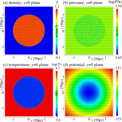
Figure 1: Initial conditions in the Model 1 simulation. Raw data are available from https://doi.org/10.5518/897.

In this work, the magnetic field is included, and the question of whether thermally unstable material can ever lead to star formation under only the influence of magnetic field and self-gravity explored for an extended range of cloud sizes (and hence masses), external medium conditions and magnetic field strengths. The range of conditions explored in this project are detailed in Table 1. Several individual models have been reported on previously, as noted in the final column of the table. Five models have been selected for this work, exploring whether gravitationally-collapsing clumps and cores ever form. A super-massive cloud is now included with a radius of 200 pc and a mass of $1.1\times 10^{6}$ M_⊙. A higher density external medium has also been considered, specifically n = 0.85 cm^-3. This relaxes the requirement for an over-equilibrium-pressure surrounding medium, as this density is in pressure equilibrium with the cloud, but on the warm, stable region of the equilibrium curve. The external medium is thus allowed to heat and cool. Several magnetic field strengths are also explored, corresponding to plasma beta values of 0.1, 1.0, 10, 33 and 40 - these physically correspond to $B_{0}$ = 3.63, 1.15, 0.363, 0.2 and 0.181$\mu$G. The plasma beta ($\beta_{\rm plasma}$) value indicates the ratio of thermal pressure to magnetic pressure, thus these values can be considered as initially magnetically dominated ($<$1.0), equipartition (1.0) and thermally dominated ($>$1.0). Various domain sizes and resolutions are employed in order to elucidate the interplay of magnetic field and thermal instability. Further to the list of production simulations in Table 1, extensive resolution, physical parameter and process tests have been performed during the project to ensure correct capture of the effects in question.

A slice through the centre of the domain in Model 1 is shown in Fig. 1. Model 3 is almost identical in appearance, except that the domain and cloud radius are four times as large and the external medium density has the second value of 0.85. An amended scaling ratio in the code is used to allow the cloud to extend only to 1 in code units, but a higher resolution employed to allow comparison with earlier Models. Model 5 concerns an extracted central section from Model 3, initialised in a very similar manner to the study reported in Paper V. A central spherical region of Model 3, radius 50 pc, was placed in a cube domain 120 pc on a side. The stationary surroundings outside the spherical region were pressure and density matched to those low-density surroundings inside the region in the same manner as Paper V. A uniform magnetic field, equivalent to the field strength in and around the sheet measured from Model 3, was inserted across the domain. Model 5, with initially 5 levels of adaptive mesh refinement (AMR), matched the finest levels of resolution with Model 3, but as Model 5 was evolved, extra levels of AMR were rapidly added to accurately resolve the formation of massive clumps, resulting in the finest resolution as described in Table 1.

3 Numerical methods and model

The MG MHD code has been used here in the same manner with the same heating and cooling prescriptions as throughout Papers I to V and for reasons of brevity, we ask the interested reader to consult those papers for further details.

Table 1: Details of the suite of 3D Cartesian MHD simulations, including heating, cooling and self-gravity, performed during the program of work reported in Papers I-V and herein. Individual simulations discussed in this work are given specific Model names. Specific citations are given to simulations discussed in preceding publications.

Name	Physical	Cloud	Cloud	Initial	$\rho_{\rm{surr.}}$	G0	Max.	Finest	References/Comments
herein	Domain	Radius	Mass	$\beta_{\rm{plasma}}$	n		levels	Res.
	[pc on a side]	$R_{init}$ [pc]	[M⊙]		[cm-3]	[# of cells]	AMR	[pc]
	150	50	1.7e4	0.1	0.1	$4\times 4\times 4$	8	0.29	See Paper I
Model 1	150	50	1.7e4	1.0	0.1	$4\times 4\times 4$	8	0.29	See Papers I and II
	150	50	1.7e4	10.0	0.1	$4\times 4\times 4$	8	0.29
	150	50	1.7e4	1.0	0.85	$4\times 4\times 4$	8	0.29
	150	50	1.7e4	10.0	0.85	$4\times 4\times 4$	8	0.29
	150	50	1.7e4	33.0	0.85	$4\times 4\times 4$	8	0.29
Model 2	300	100	1.35e5	1.0	0.1	$8\times 8\times 8$	8	0.29	See Paper IV
	300	100	1.35e5	10.0	0.1	$8\times 8\times 8$	8	0.29
	300	100	1.35e5	1.0	0.8	$8\times 8\times 8$	8	0.29
	300	100	1.35e5	10.0	0.8	$8\times 8\times 8$	9	0.14
	600	200	1.1e6	0.1	0.85	$6\times 6\times 6$	8	0.78
Model 3	600	200	1.1e6	1.0	0.85	$6\times 6\times 6$	9	0.39
Model 4	600	200	1.1e6	10.0	0.85	$6\times 6\times 6$	9	0.39
	600	200	1.1e6	40.0	0.85	$6\times 6\times 6$	8	0.78
Model 5	120	50	1.38e5	$\sim 1.0,$	0.385	$12\times 12\times 12$	8	0.078	Extracted from Model 3
		(disc)		up to 2.8					after collapse to a disc
				at high $\rho$					$t_{\rm start}$=50.1 Myrs

Table 1 presents details of the simulations presented in this work. The simulations employ a varying base AMR grid (G0) and varying levels of AMR. The finest grid resolution is typically 0.29 pc, increased to 0.078 pc for the high-resolution study of collapsing cores to be comparable to Paper V. G0 needs to be coarse to ensure fast convergence of the MG Poisson solver. It should be noted that here, as in our previous papers, we do not include thermal conductivity, nor do we resolve the Field length in the manner discussed by Koyama & Inutsuka (2004). As we show in a convergence study and discussion in Appendix A, it is not strictly necessary to do either of these things, if we are only concerned with the large-scale behaviour of the thermal instability, which is convergent at such scales. Any small-scale structure introduced by not including thermal conductivity is subsumed into the larger structure.

The central region of the Model 3 simulation was extracted in order to provide the initial condition for resimulation in Model 5. Mapping of the region extracted from Model 3 onto Model 5 was performed in a simple linear fashion over all three coordinate directions for every cell in question. The dense sheet structure in this grid was well-resolved (by 10 or more cells) in order to ensure no loss of detail. Model 5 started with 5 levels of AMR, but extra levels were added as the structure reached resolution limits for each level, up to 8 levels of AMR. The simulations were typically run across 96 cores of the ARC HPC facilities at the University of Leeds, including some of the final available cycles of the long-lived and well-used DiRAC1 UKMHD machine that has been particularly beneficial to this project (see also the Acknowledgments).

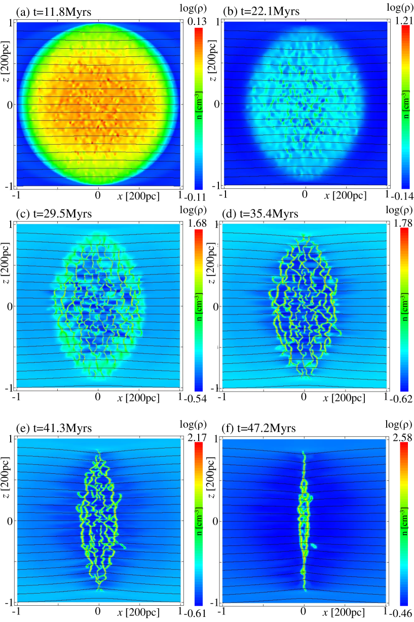
Figure 2: The evolution of Model 3. Number density slices through the $y=0$ plane are shown with magnetic field lines. Raw data are available from https://doi.org/10.5518/897.

4 Results and Discussion

Cloud structure and evolution are discussed in this section. In particular, time-variation of properties, derived statistics, slices and column density projections at snapshots in time are examined. MG plotting mechanisms and in-house software are used to visualise these data.

4.1 Evolution

The evolution of the Model 1 cloud is discussed in detail in Paper I, where figs. 4, 5, 6 and 7 illustrate the evolution. This evolution can be summarised as follows. From the unstable initial condition, as is shown for Model 3 in Fig. 2, over-dense thermally stable, cold condensations begin to appear after approximately 20 Myrs (Fig. 2b), alongside regions of diffuse, stable warm medium. Thermal motions of the gas along the field-lines accompany this phase. The collapse of the cloud under gravity leads to greater sub-Alfvénic motions along the field-lines toward the minimum of gravitational potential along that field line, in agreement with the theoretical predictions and simulations (Girichidis et al., 2018). Magnetic pressure supports the cloud across the field lines. Condensations appear to grow across the field-lines (Fig. 2c), but this is the result of material collecting through motion along the field-lines, not motion across the field-lines. This has the effect of increasing density in some locations and creating low-density field-aligned structure in others, resembling striations inside and outside the cloud (Fig. 2d). Note the consistent appearance of such structure in the convergence tests shown in Appendix A. The cloud resembles a transitory foam-like structure (Fig. 2e) on the way to collapsing to a thick, corrugated, approximately circular sheet after 40 Myrs, with a radius the same as the initial condition (Fig. 2f). In projection, the corrugations across the sheet can appear to give an integral-shaped morphology, as demonstrated by Model 2 and discussed later. The sheet radius is 50 pc in the case of Model 1 and 100 pc in the case of Model 2. If enough mass is present in the sheet for gravity to overcome the magnetic pressure support, the cloud then globally collapses across the field lines at the same time as approaching a thick sheet-like configuration. Model 1 does not collapse across the field lines, whereas Models 2, 3 and 4 do to lesser (Model 3) and greater (Models 2 and 4) effect. This process intensifies the magnetic field, resulting in hourglass field morphology (discussed later in more detail for Model 4). If enough mass is present locally (originally in the column along the magnetic field line), then magnetic supercriticality can be achieved locally and gravity overcomes the magnetic support leading to gravitational collapse of the clumps into cores on a shorter free-fall time-scale than that of the whole cloud. This is demonstrated in Model 3 and at a higher resolution by Model 5.

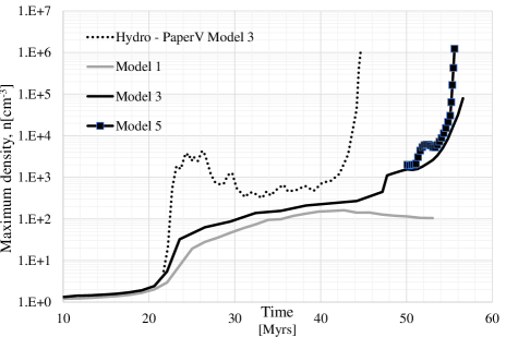
Figure 3: The evolution of the maximum density. Presented are the collapsing HD case from Paper V and a number of the MHD cases: the low mass magnetic cloud (Model 1), the high-mass cloud (Model 3) and the resimulation of an extract of the high-mass cloud at higher resolution (Model 5). Raw data are available from https://doi.org/10.5518/897.

Fig. 3 shows the evolution of the maximum density in the simulations - a simple way to track if the cloud creates clumps and cores, or remains quiescent. For reference, Fig. 3 shows the behaviour of the purely HD case that creates clumps and cores in the case of no magnetic field, detailed in Paper V. In this HD case, there is a phase of evolution where there are reasonably high peaks in the maximum density (23-30 Myrs), but as noted in detail in Paper V, the dynamics of the cloud overcome any possibility of forming truly bound and collapsing clumps until later. Characteristic of this phase is a network of clumps connected by filaments. Both clumps and filaments display properties that compare well to observations, specifically filament widths, temperatures and flow characteristics and clump size-scales, masses, temperatures and velocity dispersions. For the details of these comparisons, please refer to Paper V. Turning now to the MHD cases, it is first reassuring to note that the HD and MHD models are converged until approximately 22 Myrs, capturing the initial evolution of the thermal instability. The HD and MHD cases then diverge. There is no phase of dynamic evolution in either of the low mass (Model 1) or high mass (Model 3) MHD cases. Any formation of a filamentary network is suppressed. The thermal flow that condensed the thermally stable structure in the HD case is now confined to 1D along the field lines by the magnetic pressure. Both magnetic cases follow a similar evolution until approximately 40 Myrs. Model 1 does not have sufficient mass to either globally collapse across the field lines under the effect of gravity, or for the formation of individual clumps across the sheet. However, Model 3, with 64 times more mass than Model 1 (see Table 1) clearly does have enough mass to overcome the magnetic support and collapse. The collapse of the cloud continues with the same power-law index (constant gradient in the plot), in terms of maximum density increase with time, until with enhanced resolution, Model 5 reveals the collapse of individual clumps to high density. The power-law indices (gradients) of the HD and MHD cases are very similar: compare the period of the HD case between 34 and 40 Myrs to that of the MHD case between 30 and 45 Myrs. Note also that both require regions with density over 1000 cm^-3 before clumps can collapse. Above this density, both HD and MHD cases display similar clump collapse time-scales in this figure, albeit occurring at 54-56 Myrs in the MHD case as compared to 42-44 Myrs in the HD case. Clearly in the HD case, the nature of the cloud evolution unconstrained by the magnetic field leads to flows in any direction and collapse to higher density on a shorter timescale, even if there is a period where the thermally-induced flows prevent gravitational collapse. Gravity now dominates the final evolution in both the HD and high-mass MHD cases.

To understand why Model 3 collapses and Model 1 does not, we now explore the critical differences between the models. The initial cloud is in an unstable equilibrium state. On the timescale of approximately 20 Myrs (Fig. 2b) it evolves into a thermal equilibrium state containing dense, cold stable material and diffuse, warm stable material in pressure equilibrium, as also illustrated in fig. 2 of Paper V. The final evolutionary outcome can be illuminated by considering the equilibrium state produced by the collapse of a uniform, non-rotating, isothermal, spherical core as considered by Mouschovias (1976a, b) and later in terms of MHD shocks and subcritical cores relevant to this work by Vaidya, Hartquist & Falle (2013). Specifically, for a zero-temperature core, Mouschovias & Spitzer (1976) derive the critical value of mass-to-flux ratio above which a core will collapse under gravity as

$$\frac{{{M_{\rm crit}}}}{{{\Phi_{\rm crit}}}}=\frac{{0.53}}{3\pi}{\left({\frac{5}{G}}\right)^{1/2}}.$$ (1)

Vaidya, Hartquist & Falle (2013) note that for the case of ideal MHD the mass-to-flux ratio does not change and this becomes

$$\frac{M}{\Phi}=\frac{{4{\rho_{i}}{R_{i}}}}{{3{B_{0}}}}.$$ (2)

Thus, in this case with a constant density for all initial conditions within the thermally unstable range, there is a critical initial cloud radius, below which the cloud will not collapse, given by

$${R_{crit}}=\frac{{3{B_{0}}}}{{4{\rho_{i}}}}\frac{M_{\rm crit}}{\Phi_{\rm crit}}.$$ (3)

For $\rho_{i}=1.1$ cm^-3 and $\beta_{\rm plasma}=1.0$ resulting in B₀=1.15 $\mu$G, we obtain R_crit=73 pc. Model 1, with a radius of 50 pc, is therefore sub-critical. Models 2, 3 & 4 are supercritical and will eventually collapse.

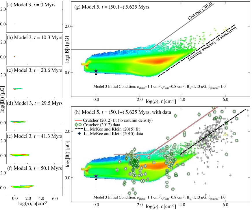
Figure 4: Comparison of Models 3 and 5 to observational data, fits and another simulation concerning the relationship between magnetic field strength and data. Panels (a) to (f) show the evolution of the distribution for Model 3. Panel (g) shows a comparison between Model 5 and the Bayesian fit for maximum field strength presented by Crutcher et al. (2010) and Crutcher (2012). The dashed line shows the indicative limiting power-law trend of the minimum field strength for a certain density in the simulation. Panel (h) shows the same Model 5 distribution as in (g), but overlaid with the Bayesian fit and data used to obtain the fit (Crutcher, 2012), as well as simulated data and a fit from the turbulent simulations of Li et al. (2015). Raw data are available from https://doi.org/10.5518/897.

Crutcher (2012) showed (in their fig. 6) the application of a Bayesian statistical technique to analyze samples of clouds with Zeeman observations (Crutcher et al., 2010). The model assumed that the maximum magnitude of the magnetic field was independent of density up to a certain value of density. The Bayesian analysis fit to observational data from four surveys for the Zeeman, Hi, OH and CN data revealed the maximum magnetic field strength to be approximately B${}_{0}\sim$ 10$\mu$G up to approximately n${}_{0}\sim$ 300 cm^-3 (n(H${}_{2})\sim 150$ cm^-3). Above this, maximum field strength was assumed to have a power-law increase, which was found to be of the form B $\propto$ B₀(n/n₀)^0.65, indicative of isotropic contraction and magnetic supercriticality. More recently, Tritsis et al. (2015) found a power-law index of $\sim 0.5$ indicative of one-dimensional collapse along fieldlines based on an analysis of a limited set of Zeeman data and Kandori et al. (2018) found an index of $0.78\pm 0.10$ toward the starless dense core FeSt 1-457.

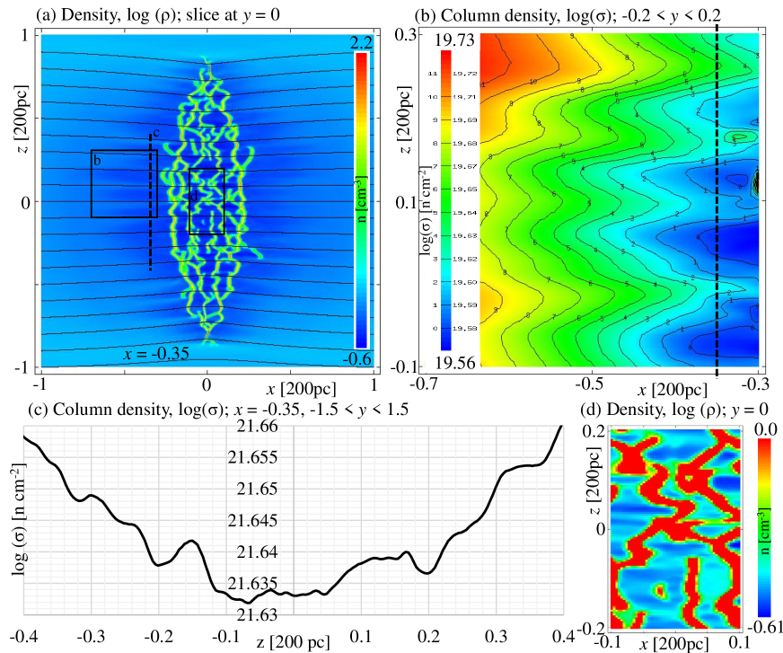
Figure 5: The appearance and properties of striations closely-aligned to the magnetic field in Model 3 after 41.3 Myrs of simulated evolution. Panels (b), (c) and (d) show the column density for the regions marked ’b’ and ’d’ and the line marked ’c’ in panel (a). Raw data are available from https://doi.org/10.5518/897.

In Fig. 4, we now explore the behaviour of the simulations with respect to the Crutcher (2012) relationship. Fig. 4 shows the magnetic field strength versus density distribution for Model 3 and its high resolution resimulation in Model 5. In the colour distribution plots, every cell in the grid simulation has been accounted for and the colour scale indicates the frequency of cells with such magnetic field and density properties, from blue indicating very few cells to red indicating a large number of cells. Given that the initial magnetic field strength is constant and the initial density only varies over a narrow range, the distribution of the initial condition as shown in Fig. 4a is very confined. Over the next 50 Myrs as shown in panels a to f (the entire duration of Model 3) the major effect on the distribution is a rightwards spread - a range in density of more than 3 orders of magnitude, but very narrow range of slightly increased magnetic field strength. As can be seen in Fig. 4f, increasing density above a certain level is then also accompanied by increasing magnetic field. It is interesting to note that this density threshold (300 cm^-3) is the same as that at which Crutcher (2012) deduced a switch from a flat maximum magnetic field strength to a power-law relationship between maximum magnetic field strength and density. Only when gravitationally unstable regions appear and collapse to high densities does the magnetic field strength increase with density, as can be seen in Fig. 4g. The simulations appear to show the same tendency to a power-law increase with the same gradient index. The distribution falls reassuringly below Crutcher’s maximum field strength relationship. It should be noted that different initial conditions - specifically an initial magnetic field greater than 10 $\mu$G in the thermally unstable medium - would result in a distribution above Crutcher’s relationship at densities below 10³.

It is notable, as shown in Fig. 4h, that when the observational data are included (green circles and diamonds), the spread of the data is wide and encompasses the simulated distribution. The peak of the simulated distribution is in good agreement with the majority of the observational data. The black crosses fit by the dashed line in Fig. 4h are the simulated data and fit of Li et al. (2015), who consider the turbulent formation of molecular clouds. They conclude the results of their strong field model (Alfvén Mach number of 1) are in very good quantitative agreement with observations. On this point in particular, their work is in good agreement with our simulated distribution at high density, even though they start from a very different premise of turbulence-driven molecular cloud formation. Crutcher (2012) derives the relationship as the limiting relationship between magnetic field and density and it would appear that this is indeed the case.

Everything together in Fig. 4h - data, fit to data and two simulations from very different initial conditions - seems to agree well with the conclusions of Crutcher (2012): specifically, that magnetic field morphologies appear to be generally smooth and coherent across the range of scales considered here from 10² to 10^-2 pc. However it should be noted that we impose a smooth initial magnetic field in our initial condition. Ordered fields perpendicular to elongated structures suggest contraction along magnetic field lines. Data, both observational and simulated, seems generally consistent with the scenario that molecular cloud complexes are formed by accumulation of matter along magnetic flux tubes, such that the magnetic field does not increase much with density up to n $\sim 300$ cm^-3. Above this density, Crutcher (2012) concludes, magnetic field strengths increase with increasing density, with a power-law exponent indicating that gravity dominates magnetic pressure. Our simulations indeed become dominated by gravity above this density in precisely this manner, providing some clarity of the astrophysical processes at work which can reproduce the observations.

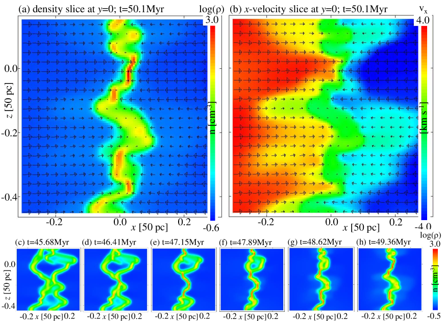
Figure 6: The appearance of integral-shaped structure and the associated velocity field in Model 2. Reversals in velocity vector over short distances close to the dense structure are apparent in panel (a), whilst the colour map of panel (b) demonstrates the red/blue-shift effect on either side of the dense structure. Panels (c) to (h) illustrate the timescale and motion of collapse. Raw data are available from https://doi.org/10.5518/897.

4.2 Striations

In Fig. 5, an example of the striations that form around the dense cloud structure is presented. Fig. 5a shows a slice through the centre of the simulation domain of Model 3, where striations - low-density, field-aligned structure - can be seen outside the dense regions of the cloud. These striations are in the low-density warm diffuse medium: their density is below n $\sim 1$ cm^-3. In these simulations, at this resolution, they do not contain any cold, dense material. Figs 5b and 5c show the typical column density variation across these striations. The average difference peak to trough in column density is around 10-15%, but this does range up to 25% just in the panel shown here. Note that the column density in Fig. 5c is larger than that in Fig. 5b as this cut takes account of the depth of the entire simulation box (3 in code units), so the variations peak to trough are smaller in terms of percentage difference given as they appear as a variation on this background created by the whole domain, but the column density in panel c is in agreement with the range observed around n${}_{\rm H}\sim 10^{21}$ cm^-2 for structure in Taurus at a distance of $\sim$120 pc (Goldsmith et al., 2008; Tritsis & Tassis, 2016).

It should also be noted that low-density striations are also found in the centre of the Model 3 simulated cloud, as shown in Fig. 5d, and across the entire range of magnetic simulations performed during this project (see Table 1, Papers I, II and IV). Such striations are essentially the same as those outside the cloud, though they are not physically connected. It is clear from Figs 5a and 5d that the low-density striations are associated with structure in the dense filaments e.g. local high densities or intersections of filaments. We also find that the striations only appear after that of dense structure, which suggests that they are generated by the thermally-induced flows that cause the dense structures; compare panels (c) and (d) of Fig.2 and note the material trailing from the accretion that remains collimated along the field-lines. This interpretation is supported by the velocity structure of the striations, indicating the remnant of the accretion flow. This could be due to the same mechanism of MHD waves discussed by Tritsis & Tassis (2016) for high density striations, as the comparatively long-lived low-density striations in the magnetic simulations are clearly magnetically controlled (as opposed to those that appear briefly in the purely hydro simulations in Paper V, show no preferred direction and lead to the filaments that connect clumps). Further work is required to explore this possibility, but the presence of low-density striations in simulations with and without self-gravity, with and without periodic domains (see Appendix A and Paper I for such periodic simulations), lends credibility to an origin in the thermal instability.

In general, the MHD simulations indicate a preference for low-density structure (striations) to align parallel to the magnetic field and high-density structure (sheets) to orient perpendicular to the magnetic field. This is in agreement with observations, such as a Mopra telescope survey of molecular rotational lines towards the young giant molecular cloud Vela C (Fissel et al., 2019) which quantified the orientation of gas structure with respect to the cloud magnetic field orientation. Those authors estimate the characteristic transition density from parallel to perpendicular to be around $10^{3}\pm 10^{1}$ cm^-3, similar to what we observe in our simulations. However, we must stress that the striations we observe in our simulations are not the same as those dense, cold striations observed in CO emission and modelled by Tritsis & Tassis (2016). Our diffuse, warm striations are more likely to be linked to the elongated fiber structures observed at high Galactic latitudes in the diffuse interstellar medium, referred to by Tritsis & Tassis (2016).

It is possible that AMR can produce striation-like grid-aligned structure, if a faulty grid control algorithm is present and careful consideration of the results is not employed. We have seen this in other applications outside astrophysics and responded by reconsidering the grid control algorithm and repeating the calculations. No such amendments have been necessary in the suite of simulations presented in this series of papers. The striations are well-resolved perpendicular to their orientation by 5 to 10 cells. Their initial appearance in the simulations follows the appearance of thermally-stable structure, not any changes in grid resolution in that local area. Their appearance is also common at the same size-scale across our results presented herein, the convergence tests presented in Appendix A with and without thermal conductance and across the suite of simulations in Papers I, II and IV as already noted.

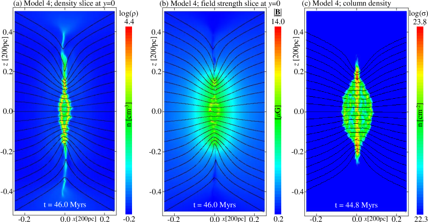
Figure 7: Demonstration of global cloud collapse and formation of hourglass-like field structure in Model 4. The initial simulation had a uniform magnetic plasma beta of 10 across the domain. At the times presented, the plasma beta now varies across the simulation volume and realistic values of field magnitude (5-10 $\mu$G) and plasma beta ($\sim 1$) are obtained in the high density cloud regions, regardless of the initial condition. In projection (c), two approaching ‘clumps’ appear to be dragging the field akin to recent observations in OMC1 (Pattle et al. 2017). Raw data are available from https://doi.org/10.5518/897.

4.3 Integrals

In the simulations, the thick disc-like molecular clouds have a natural corrugation which appears as an integral-shape in cross-section and projection. The disc briefly oscillates about the potential minimum along the field lines, with a standing wave nature perpendicular to the magnetic field and a peak-to-peak distance set by the size-scale of 5-10 pc that results from the thermal instability (Falle et al., 2020). Fig. 6 shows this effect in the Model 2 simulation once the cloud has collapsed to a sheet but before the disc reaches static equilibrium at the minimum of the gravitational potential. This is a transient effect of ‘collapse-overshoot’ as the material flows non-uniformly along the fieldlines into the gravitational potential well as a result of the thermal instability. The velocity range is not insignificant, from -4 to +4 km s^-1 as shown in Fig. 6b. These structures and the disconnects in velocity are similar to those presented in Stutz et al. (2018) and González Lobos & Stutz (2019) concerning a wave-like model for the ISF in Orion A. Clearly there is a realistic physical formation mechanism for such structure and velocity patterns, deriving from the thermal instability and leading to interaction between magnetic field and gravity. Similarly, it is therefore possible that the ‘vibration’ of Musca detected by Tritsis & Tassis (2018) is an effect of gravitational contraction and oscillation about the potential minimum over a period of Myrs (panels (c) to (h) of Fig. 6), with striations formed in the manner discussed above. Further work to investigate this is required.

Interestingly, Liu et al. (2019) investigate the internal gas kinematics of the filamentary cloud G350.54+0.69 and find a large-scale periodic velocity oscillation along the filament, with a wavelength of 1.3 pc and an amplitude of $\sim$0.12 km s^-1. The authors conjecture the periodic velocity oscillation could be driven by a combination of longitudinal gravitational instability and a large-scale periodic physical oscillation along the filament, possibly an example of an MHD transverse wave. It’s clear that during the collapse of a thermal instability driven cloud, the resulting velocities encompass this observation. In our simulations, the velocity range reduces over time as the amplitudes of the oscillation reduce due to the sheet reaching the potential minimum. Our model and the observations of Liu et al. (2019) are therefore compatible.

In addition, Shimajiri et al. (2019) concluded from red-shifted and blue-shifted velocity patterns around the Taurus B211/B213 filament that the filament was initially formed by large-scale compression of Hi gas and is now growing in mass by gravitationally accreting molecular gas from the ambient cloud. The simulations show similar global red-shifting and blue-shifting patterns on either side of the molecular structure, as can be inferred from the velocity patterns in Fig. 6b. The observed shifted velocities around the Taurus B211/B213 filament are on the order of 1-2 km s^-1 - well within the range of velocities that we see in our simulations.

In summary, the gravitational collapse of a cloud triggered by thermal instability produces a cloud with a converging flow which is similar to models involving colliding flows. However, they do not represent large-scale converging flows, but instead are a natural consequence of the thermal instability combined with gravity. This work now adds a further possibility of thermal flow origins to such observed velocity patterns and structures.

Table 2: Properties of the 33 clumps identified by the FellWalker algorithm, at t=55.6 (50.1 + 5.5) Myrs in the Model 5 simulation. Snapshots of slices through the clumps are available from https://doi.org/10.5518/897.

	Mtotal	Mwarm	Munstable	Mcold	$\rho_{\rm max}$	Tmin	Scale	vdisp	Bound?	Jeans
	[M⊙]	[M⊙]	[M⊙]	[M⊙]	n [cm-3]	[K]	[pc]	[km s-1]		unstable?
1	1.98e3	5.81e0	3.24e0	1.98e3	4.41e3	16.4	4.0	0.27	N	N
2	1.78e3	4.35e0	3.21e0	1.77e3	9.42e3	14.7	2.0	0.26	N	N
3	8.19e3	9.28e0	1.56e1	8.18e3	5.20e3	19.8	2.0	0.12	Y	Y
4	1.41e3	2.00e0	2.72e0	1.40e3	2.60e4	12.8	1.0	0.28	Y	Y
5	1.47e3	4.36e0	2.37e0	1.46e3	1.24e6	8.1	2.0	0.73	Y	Y
6	3.01e3	9.26e0	5.48e0	3.00e3	1.40e4	13.9	3.0	0.28	Y	Y
7	2.49e3	2.55e0	4.49e0	2.49e3	3.13e3	17.6	2.0	0.21	Y	Y
8	3.69e3	6.65e0	7.26e0	3.68e3	2.94e3	17.8	3.0	0.19	Y	Y
9	2.88e3	5.08e0	5.28e0	2.88e3	3.22e3	18.1	3.0	0.15	N	N
10	1.63e3	2.48e0	3.45e0	1.62e3	2.57e3	18.6	5.0	0.17	Y	Y
11	2.85e3	3.83e0	5.08e0	2.85e3	3.03e3	17.7	2.0	0.17	N	N
12	1.76e3	2.09e0	3.48e0	1.75e3	7.83e3	15.1	1.5	0.20	Y	Y
13	1.72e3	2.02e0	3.49e0	1.72e3	1.46e4	13.8	1.5	0.22	Y	Y
14	7.46e2	8.15e-1	1.41e0	7.44e2	3.15e4	12.6	1.0	0.26	Y	Y
15	2.36e3	2.07e0	4.73e0	2.35e3	6.25e3	15.7	1.5	0.23	N	N
16	3.43e2	3.24e-1	6.84e-1	3.42e2	5.86e3	15.9	3.0	0.23	N	N
17	3.97e3	5.55e0	7.57e0	3.97e3	7.64e3	15.1	3.5	0.23	Y	Y
18	1.36e2	7.53e-2	2.01e-1	1.36e2	2.14e3	18.3	3.0	0.21	N	N
19	9.44e2	1.21e0	2.05e0	9.41e2	4.41e3	15.0	2.0	0.24	Y	Y
20	5.82e2	4.87e-1	9.52e-1	5.81e2	3.86e3	15.7	1.5	0.26	N	N
21	1.30e3	1.22e0	2.70e0	1.30e3	2.47e3	18.7	3.0	0.26	N	N
22	2.85e3	3.80e0	5.51e0	2.85e3	3.11e3	17.7	4.0	0.18	Y	Y
23	2.44e3	2.55e0	4.46e0	2.44e3	6.28e3	15.7	4.0	0.23	N	N
24	1.39e3	1.34e0	2.77e0	1.39e3	6.85e3	15.5	2.0	0.20	Y	Y
25	5.66e3	1.11e1	1.12e1	5.65e3	9.56e3	14.6	2.5	0.28	Y	Y
26	4.06e3	6.26e0	8.48e0	4.05e3	6.31e3	15.8	3.0	0.34	Y	Y
27	2.20e3	2.61e0	3.91e0	2.20e3	7.72e3	15.1	1.5	0.24	Y	Y
28	3.87e2	5.72e-1	7.01e-1	3.86e2	2.07e3	14.5	2.0	0.26	Y	Y
29	2.78e3	3.84e0	5.75e0	2.78e3	1.35e4	14.0	2.0	0.23	Y	Y
30	4.81e3	9.36e0	9.32e0	4.81e3	5.76e3	15.5	3.0	0.28	Y	Y
31	3.66e3	4.60e0	6.79e0	3.66e3	3.22e3	19.1	4.0	0.32	N	N
32	3.42e2	3.93e0	3.78e-1	3.42e2	7.41e3	15.2	3.0	0.26	N	N
33	1.68e3	3.84e0	2.77e0	1.67e3	4.42e3	16.7	4.0	0.40	N	N

4.4 Hourglasses

Fig. 7 shows slices through and column density projections of the Model 4 simulation in order to demonstrate the formation of hourglass field morphologies and the strengthened magnetic fields. Model 4 was initialised with $\beta_{\rm plasma}=10.0$ resulting in a uniform magnetic field with magnitude of $0.363\,\mu$G. The radius of the initial cloud in code units was 1.0. In this magnetically weak case, the disc-like cloud has collapsed across the magnetic field lines under the influence of gravity. As can be seen in Fig. 7a, after 46 Myrs the cloud has collapsed to a radius of $\sim 0.2$ in code units. For comparison, the Model 3 cloud with an initial $\beta_{\rm plasma}=1.0$ has only shrunk slightly perpendicular to the magnetic field after a similar period of evolution (as shown in Figs. 2e and 2f). The result of the collapse in Model 4 is still a disc-like cloud, but with a much smaller radius than the initial condition and an intensified magnetic field as shown in Fig. 7b. Across the denser regions of the cloud ($r<0.15$) the magnetic field now averages 5 to 7$\,\mu$G. Some of the densest locations have field intensifications up to $14\,\mu$G, approximately $40\times$ stronger than the initial field. Values of $\beta_{\rm plasma}$ are around unity, corresponding to observational estimates in real molecular clouds. This demonstrates that although the initial condition may not have a realistic value of $\beta_{\rm plasma}$, the resulting molecular cloud and dense condensations do have realistic properties.

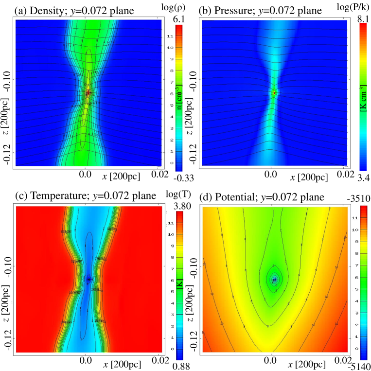
Figure 8: Properties of Clump 5, the highest-density collapsing clump in the Model 5 simulation at t=55.6 Myrs. Shown are density, pressure, temperature and gravitational potential on the plane at $y=0.072$, perpendicular to the sheet. Magnetic field lines are indicated on the density and pressure plots. Raw data are available from https://doi.org/10.5518/897.

Fig. 7c shows a column density projection at a slightly earlier time, with magnetic field lines from the slice $y=0$ superimposed, as per the other panels in this figure. In projection, this has the appearance of two dense clumps approaching each other, dragging the magnetic field lines with them. This is very reminiscent of the hourglass morphology of the magnetic field in the OMC1 region of the Orion A filament where two clumps appear to be approaching each other and creating an hourglass magnetic field configuration (see details in and fig. 1 of Pattle et al., 2017). This demonstrates the capability of the physical model to create intensified fields, with hourglass field morphologies, that still preserve the large-scale ordered magnetic fields in the diffuse surroundings, albeit as a remnant of the initial condition. Other models also present field amplifications in the densest regions, e.g. similar values of the magnetic field in the densest clump formed in Model 5 discussed in Sec. 4.5.1. The hourglass magnetic field configuration compares well to observations, for example in Kandori et al. (2017), who derive the magnetic field configuration around the starless dense core FeSt 1-457.

4.5 Clumps

We now consider the high-resolution Model 5 resimulation of the central section of Model 3 and identify any massive clumps that have formed. The FellWalker clump identification algorithm (Berry, 2015) has been implemented into MG in order to do this. The implementation, testing and application to the HD case is described in detail in Paper V.

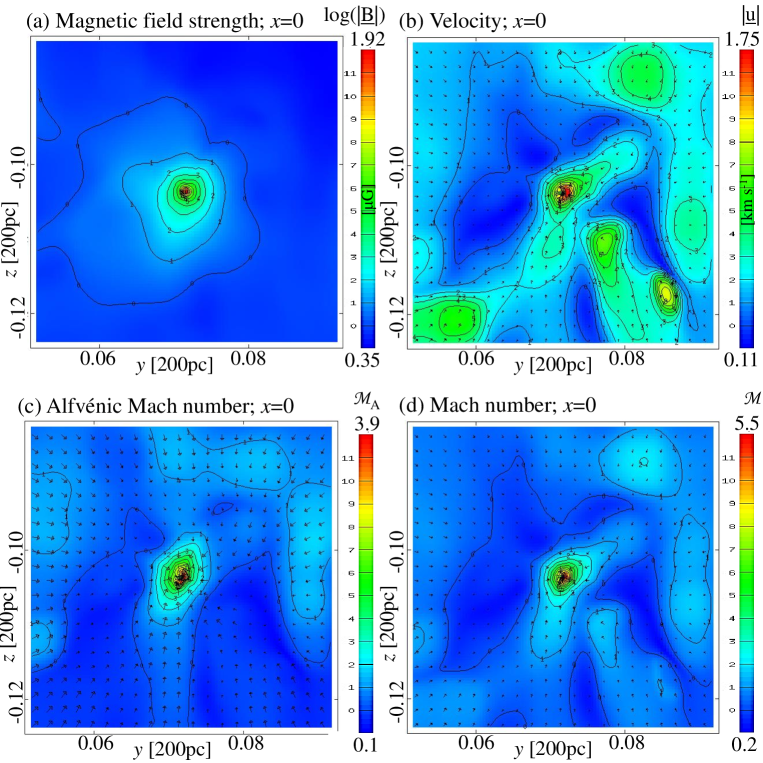
Figure 9: Further properties of Clump 5, the highest-density collapsing clump in the Model 5 simulation. Shown are magnetic field strength, velocity, Alfvénic Mach number and flow Mach number on the plane at $x=0$, parallel to the sheet. Velocity and Mach numbers are shown in the frame of the clump, not the simulation. Raw data are available from https://doi.org/10.5518/897.

FellWalker has been applied to the Model 5 simulation after 5.5 Myrs of evolution. This is in addition to the preceding 50.1 Myrs of evolution of Model 3. The algorithm detected 33 clumps, detailed in Table 2, 20 of which are gravitationally unstable (E${}_{\rm grav}>$ E_th + E_kn + E_mag). At this time the highest density in the simulation, in the collapsing core of Clump 5, has reached the point at which it the resolution should be increased by adding other level of AMR. However, this is a good point to analyse the simulation since we have a reasonable number of gravitationally bound clumps and the computational expense of extra AMR levels is very high.

Bergin & Tafalla (2007) review the properties of clumps based on Loren (1989) and Williams, de Geus & Blitz (1994): mass 50-500 M_⊙; size 0.3-3 pc; mean density 10³-10⁴ cm^-3, velocity dispersion 0.3-3 km s^-1; sound crossing time 1 Myr; gas temperature 10-20 K. These values fit those of the 33 clumps very well, except that the clumps are rather more massive. In each clump, the majority ($>95\%$) of the mass is in the cold phase. Minimum temperatures, which occur in the inner regions of each clump where the lowest velocity dispersion also occurs, are in good agreement with Bergin & Tafalla’s review. Images of the clumps can be found in the accompanying data archive at https://dx.doi.org/10.5518/897. The majority of the clumps are approximately spherical.

4.5.1 Clump 5 - an individual clump with a collapsing core

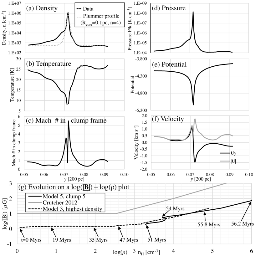
Figure 10: Properties of the highest-density collapsing clump in the Model 5 simulation, #5 in Table 2. Profiles are cuts along $y$ through the central position of the clump. The bottom graph shows the track of the clump in magnetic field strength versus density as it evolves with time. Raw data are available from https://doi.org/10.5518/897.

Turning to examine an individual clump in more detail, Figs. 8 and 9 show slices through Clump 5 and its collapsing core. The slices and profiles are cut through the position of the gravitational potential minimum of the clump, at (x, y, z = 9.77e-04 (0.19 pc), 7.17e-02 (14.3 pc), -1.04e-01 (-20.8 pc)) in the grid from -60 pc to +60 pc in all three directions. Fig. 8a shows the remarkably regular density profile described in the previous section, on a slice perpendicular to the sheet. This is common across the clumps in the Model 5 simulation and different to the HD results in Paper V, where asymmetric and complex clumps were typical, formed by the absorption of the filamentary network and clump collisions. Fig. 8b shows the high pressure in the collapsing core of the clump, a convincing signature of gravitational collapse. Whilst Clump 5 and its collapsing core seem quantitatively different from the other clumps in Table 2, it should be noted that this is merely the first of the clumps in the simulation to undergo core-collapse. Others would do the same if the simulation was evolved further beyond this point.

Notable from the magnetic field lines shown in Figs 8a and 8b is the deformation of the field in the local area of the clump, showing the effect on the field of the gravitational collapse. Fig. 8c shows the temperature on the slice through the clump, and the deep cold well at the collapsing core of the clump, dropping to a realistic 8.1 K. The potential, shown in Fig. 8d is remarkable for its smoothness across the whole slice compared to the relative complexity apparent in density. In the context of simulated HD and MHD molecular clouds, gravitational potential is clearly useful for identification of distinct clumps with structure-finding tools such as FellWalker or CLUMPFIND. Fig. 9a shows the magnetic field on a slice now across (parallel to) the sheet and perpendicular to the initial background field, indicating that the magnetic field has been very strongly intensified from an initial value of 1.15 $\mu$G up to nearly 100 $\mu$G. This intensification and magnitude compare well to the magnetic field observations made by the BISTRO collaboration (e.g. Pattle et al., 2017; Liu et al., 2019b; Wang et al., 2019; Coudé et al., 2019; Doi et al., 2020). Similarly, the collapse under the influence of gravity has also led to large infall velocities, on the order of 2 km s^-1. This is not an unreasonable velocity compared to observations, but the more important question concerns whether this velocity is supersonic and/or super-Alfvénic. We find that it is both, as shown in Figs. 9c and 9d. Specifically, at the centre, the infall velocity has an Alfvénic Mach number up to 4 and a thermal Mach number up to 5.5. Such values appear to be comparable to observations and the kind of initial conditions used by the turbulent star formation community to initialise such simulations.

Crutcher (2012) comments that the relative importance of turbulent to magnetic energy is addressed by a number of linear polarization results. He notes that the observed column density power spectrum in several cloud complexes is best reproduced by simulations that are super-Alfvénic, but agreement in the mean alignment of fields in cores and the surrounding medium cannot be reproduced by globally super-Alfvénic cloud models. This suggests that any simulation should be sub-Alfvénic on the global scales, but transition to super-Alfvénic on the small scales of gravitational collapse. Observations of the starless dense core FeSt 1-457, including ordered field lines around the core, support the conclusion of transition from magnetic sub- to supercriticality at the boundary of the core (Kandori et al., 2018). This is a severe test of models and simulations, as noted by Crutcher, one which the model here clearly passes.

Fig. 10 shows cuts along the $y$ axis through the position of the potential minimum of Clump 5. Clump 5 has a fairly uniform density distribution. Around the central peak, this is well fitted by a Plummer-like density distribution over three orders of magnitude in density (i.e. the classic Plummer-like profile introduced by Whitworth & Ward-Thompson (2001) with an observatinally confined power-law index of 4). The fit takes a central density of n = 1.23e6 cm^-3 from the data and a minimal central flat radius of $\approx$ 0.1 pc. This is not unreasonable given the FWHM of 0.2 pc of the peak. Panels (b) to (f) of Fig. 10 show further detail of Clump 5, quantifying data presented on the slices in Figs. 8 and 9.

Fig. 10g shows the evolution of the highest density location in the Model 3 simulation and Clump 5 in the Model 5 simulation on a plot of magnetic field versus density. It is clear that for the majority of the simulated time (the first 50 Myrs), whilst the density increases, the magnetic field at the highest density location remains approximately constant - replicating the flat region of the Crutcher (2012) fit. In fact the magnetic field only begins to intensify when density reaches exactly the turning point fit by Crutcher, after approximately 47 Myrs of evolution. From that point onward, the magnetic field at the highest density location and then at the position of Clump 5, grows with a remarkably similar power-law index to that of Crutcher’s fit at high-density.

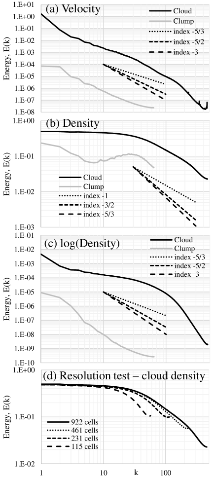
Figure 11: Instantaneous snapshot power spectra of (a) velocity, (b) density and (c) log(density) for the cloud as a whole and for Clump 5 at t=55.6 Myr. Shown in (d) is the result of interpolating data onto different levels of the AMR grid in order to demonstrate convergence. Raw data are available from https://doi.org/10.5518/897.

4.6 Power spectra

In Fig. 11, we show the snapshot power spectra of velocity and density for both the cloud as a whole and for Clump 5, at t=55.6 Myrs. The power spectra have been calculated in the same manner as in Paper V, using the same tested technique. The velocity spectra has been calculated from the complete velocity 3-vector (v_x, v_y, v_z). As in Paper V, there is no projection or smoothing of the vector into two components on a plane, as is known to affect such spectra (Medina et al., 2014). A uniform grid at the finest AMR level is used to generate the spectra, as was done but not specified in Paper V. In regions where the finest grid is not present, this was generated using the projection operator from coarser grids.

The power spectra of velocity in Fig. 11a shows that both the cloud and Clump 5 display an inertial range (region in wavenumber with slope of constant gradient) greater than one order of magnitude. The cube encompassing the cloud transformed for this analysis was 360 pc on a side. Between wavenumbers 3 and 30 (or physical scales from 120 pc to 12 pc), the spectral index is close to the Kolmogorov 5/3 spectrum generally observed in fully established turbulence over an extended inertial range covering several decades in wavenumber. We do not have that extent of inertial range, so this is not fully established turbulence, but this is very similar to the HD case in Paper V, albeit at smaller $k$ (larger physical scales). As noted in Paper V, this is also in good agreement with observationally derived velocity power spectra, for example, an index of $-1.81\pm 0.10$ derived by Padoan et al. (2006) over a similarly short inertial range (little more than one decade) for the Perseus molecular cloud complex. There is some indication of a spectral break in the cloud spectrum at $k=3$ (120 pc), which indicates flow on the scale of the cloud. At $k=30$, there is a break, beyond which the spectrum steepens to an index around -3, corresponding roughly to the separation scale of structure driven by the thermal instability, similar again to Paper V.

The velocity spectra of Clump 5 is based on a cube 10 pc on a side and so in a similar manner to Paper V, the power of the spectra is reduced by a factor 36³ in order to allow for direct comparisons between cloud and clump. In this case, the spectrum has a relatively steep initial index of -3, in agreement with cloud spectra given the maximum scale of this clump spectra is 10 pc and indicative of consistent sampling of the same physical conditions. Such an index is also consistent with that simulated by others on clump scales and below (Medina et al., 2014). The spectra also tails upwards at the smallest scales. This may be indicative of the supersonic flows at the smallest scales observed in Clump 5, but could as easily be an artefact of reaching the limits of numerical resolution as such a curl upwards at highest $k$ is typical at the limit, as we have noted before (Wareing & Hollerbach, 2009, 2010).

Although originally stated in paper V, it bears repeating here as it now also applies to the MHD case, that the stationary diffuse initial condition has generated large-scale flows with a turbulence-like -5/3 spectrum. The inertial range of the spectrum goes from cloud to clump scales (120 to 12 pc). The MHD simulations initially generate a remarkably laminar flow along the field lines, suggesting a transition towards turbulence as gravity takes over. This clearly resembles the flow and field configuration observed with such instruments as Planck, as for example shown in Paper IV around the Rosette nebula.

The power spectra of density are shown in Fig. 11b. The cloud spectrum is flat until $k\sim 30$ (12 pc) and then breaks to an index of approximately -1 from $k=30$ to $k=200$, corresponding to physical scales of 12 to 1.8 pc. On first inspection, the flat low-$k$ spectrum may be surprising. It is worth bearing in mind that along the majority of the lines through the domain with constant $y$ and $z$, parallel to the $x$ axis, the sheet is akin to a Delta function. The Fourier Transform of a Delta function is a constant. On the $x\sim 0$ plane, the sheet is approximately a top-hat function. The Fourier Transform of a top-hat function is a sinc function. A three-dimensional Fourier Transform collapsed to one-dimension in order to obtain the power spectra is thus going to be some combination of constant power and then a steep spectrum corresponding to the peaks of the sinc function. The density spectrum of the clump shows indications of the same curve up to $k=6$ as the cloud spectrum, albeit over a very small range in $k$. Then there is a wide peak around $k=25$ to 30, corresponding to the physical spherical scale of the clump potential well ($<$0.5 pc). This peak is likely to be responsible for the upturn of the whole cloud spectrum at the largest value of $k\sim 450$, as there is no corresponding upturn of the Clump 5 spectra, suggesting the simulation is well-resolved in density. The upturn would appear to be resolution independent, as shown in Fig. 11d, adding credibility to a physical origin in the smallest scales of the simulation.

Power spectra of the logarithm of density have been shown by Kowal et al. (2007) to exhibit a Kolmogorov-like behaviour when there is strong contrast of density. Those authors note that the logarithmic operation significantly filters the extreme values of the density, stopping them from distorting the spectra. Fig. 11c shows such spectra here have a spectral index in the cloud around -1 at large scales, steepening at small scales. There is no clear inertial range for the clump power spectra of the logarithm of density. It would appear that the high contrast between the dense sheet and the surroundings significantly affects the power spectrum of the clump, if less so the spectrum of the cloud. The flattening observed in density spectra is therefore due to both the sheet-like nature of the cloud and, similarly to Kowal et al. (2007), the dense small-scale structures generated across the sheet.

Apart from the size of the cloud, the only scale imposed by the initial conditions is that of the perturbation on the grid scale, which is 0.39 pc for Model 3. As in our previous simulations, there is no evidence of this scale in the spectra.

5 Summary and conclusions

The purpose of the simulations described above was to determine whether thermal instability in a diffuse cloud could produce gravitationally collapsing objects, without any other influences (e.g. turbulence) or external disturbance (pressure wave, shock or collision). Our previous work (Papers I-IV), at a lower resolution of $\geq$0.29 pc, had revealed that clumpy clouds form in the hydrodynamic case and corrugated sheet-like clouds, that in projection appear filamentary, form in the magnetic case. At high resolution, conclusive gravitational collapse has been demonstrated in the purely hydrodynamic case (Paper V). The suite of high-resolution simulations carried out here, with $<$0.4 pc resolution, up to 0.078 pc high resolution, have now conclusively demonstrated that thermal instability in a diffuse magnetic medium can generate cold and dense enough structure to allow self-gravity to take over and start the star formation process. The total time scale for this to happen is on the order of 55 Myrs, although the structure would only be considered a molecular cloud for the previous 20 Myrs.

We have noted the following:-

1. Diffuse thermally unstable material flows sub-Alfvénically along field lines and changes the spherical diffuse initial condition into a thick disc with voids and dense regions. Eventually this sheet evolves to a single, thin sheet. In the magnetically supercritical case, this sheet then collapses perpendicular to the field.

2. The relationship obtained by Crutcher (2012) is reproduced in full, both following the evolution of the whole cloud and that of a single clump. The turning point of Crutcher’s Bayesian fit at n $\sim 300$ cm^-3 is reproduced, as is the power-law gradient above that density. Agreement is shown between Crutcher (2012), observational data and Mach 10 turbulent simulations of other authors (Li et al., 2015).

3. Striation-like structure appears around the cloud and internally across the voids during the formation of the dense regions. These striations can have column densities comparable to those observed around molecular clouds, but are in the warm diffuse stable material, not cold, dense material as observed in CO emission. These diffuse striations are similar to Galactic fibres. They are not the same as the cold, dense striations observed around molecular clouds in CO emission (e.g. Goldsmith et al., 2008) and modelled by Tritsis & Tassis (2016).

4. The sheet-like molecular cloud goes through a period of oscillation about the gravitational potential minimum as it settles to its final equilibrium. During this time, the sheet resembles an integral-shaped structure, with breaks in the velocity structure along the projected filamentary structure and associated red- and blue-shifted velocity patterns. This is similar to several observational results (e.g. Stutz & Gould, 2016; González Lobos & Stutz, 2019; Shimajiri et al., 2019).

5. The gravity-dominated collapse of magnetically supercritical sheet-like clouds drags the magnetic field into an hourglass-like morphology and intensifies the magnetic field strength. The process creates field morphologies and strengths that resemble those observed (e.g., see BISTRO collaboration results: Pattle et al., 2017; Liu et al., 2019b; Wang et al., 2019; Coudé et al., 2019; Doi et al., 2020).

6. Application of the FellWalker algorithm (Berry, 2015) to a high-resolution (0.078 pc) resimulation of a portion of Model 3 finds 33 clumps with properties similar to those deduced from observations. Of these 33 clumps, 20 are confirmed to be gravitationally bound and collapsing. The densest clump has a density in its collapsing core (at the time at which the simulation is stopped) six orders of magnitude greater than the initial condition. It is collapsing on the order of a realistic free-fall time. The clump has supersonic and super-Alfvénic infall velocities, as opposed to sub-sonic and sub-Alfvénic velocities across the cloud as a whole, in agreement with the observational characteristics deduced by Crutcher (2012).

7. Velocity power spectra of the cloud as a whole and this densest clump show spectral indices that are turbulence-like (spectral index of $-5/3$) over a short inertial range (approximately one decade of wavenumber), even with the stationary initial diffuse condition. This is the result of a large-scale laminar-like flow along the field lines, with structure on small scales.

8. Velocity and density power spectra resemble turbulent initial conditions implying that 1D power spectra only offer a limited tool to discern between models of star formation.

9. The most massive clumps are found to be Jeans unstable and therefore undergo run-away gravitational collapse. Thermal instability, combined with self-gravity, is therefore able to produce collapsing clumps from a diffuse cloud, even in the presence of a dynamically significant magnetic field.

It should be noted that we have not included thermal conductivity, nor fully resolved the Field length according to the conditions set by Koyama & Inutsuka (2004). Even so, starting from highly idealised initial conditions, we still obtain convergent simulations that accurately capture the large-scale structure of the resulting thermally bistable medium. A convergence study and a full discussion of why it is not necessary to include thermal conduction, nor resolve the Field length in this case, is presented in Appendix A.

Immediate future work will now consider the effect of single star and cluster feedback in both the Paper V HD results and the MHD results presented herein, by the inclusion of a robust cluster-particle formation technique.

Data Availability

The data underlying this article are available in the Research Data Leeds Repository, at https://doi.org/10.5518/897.

Appendix A Thermal Conductivity

Field (1965) showed that, in the absence of thermal conduction, the growth rate of the condensation mode of thermal instability does not have a maximum, but increases to a finite positive limit as the wavelength tends to zero. However, thermal conduction induces a maximum in the growth rate and also stabilises modes whose wavelength is smaller than the Field length

$$\lambda_{F}=2\pi\left[\frac{\kappa T}{\rho(\rho L_{\rho}-TL_{T})}\right]^{1/2}$$ (4)

Here $\kappa$ is the thermal conductivity and $L_{\rho}$, $L_{T}$ are the derivatives of the energy loss rate per unit mass, $L$, w.r.t. density and temperature. Note that this is only defined for isobaric instability, $\rho L_{\rho}-TL_{T}>0$, and $\lambda_{F}\rightarrow\infty$ at the boundaries of the unstable region.

Koyama & Inutsuka (2004) use

$$\lambda_{F}=\left(\frac{T\kappa}{\rho L_{c}}\right)^{1/2},$$ (5)

where $L_{c}$ is the cooling rate per unit mass. This is very different from equation (4): it is significantly smaller and does not tend to infinity at the boundaries of the unstable region. Fig. 3 in Falle et al. (2020) shows a comparison between these two definitions for our energy loss rate (Koyama & Inutsuka 2002) and a thermal conductivity given by

$$\kappa=2.5\times 10^{3}T^{1/2},$$ (6)

(Parker 1953). This is due to neutrals and is therefore unaffected by the magnetic field. Note that there is an error in this figure: equation (5) is multiplied by $2\pi$.

Koyama & Inutsuka (2004) argue that simulations of thermal instability do not converge unless one includes thermal conductivity and resolves the Field length. Formally, this is true for linear perturbations, but at our initial density, $n=1.1$, the growth rate has a rather broad maximum at $\lambda=8.95$ pc (Falle et al. 2020), so there is no wavelength that is particularly favoured in the linear regime. The maximum growth rate is $0.1774$ Myr^-1, which is quite close to the zero conductivity limit of $0.1788$ Myr^-1. Koyama & Inutsuka (2004) used a somewhat higher density and a different energy loss function so that the maximum might be somewhat sharper in their case.

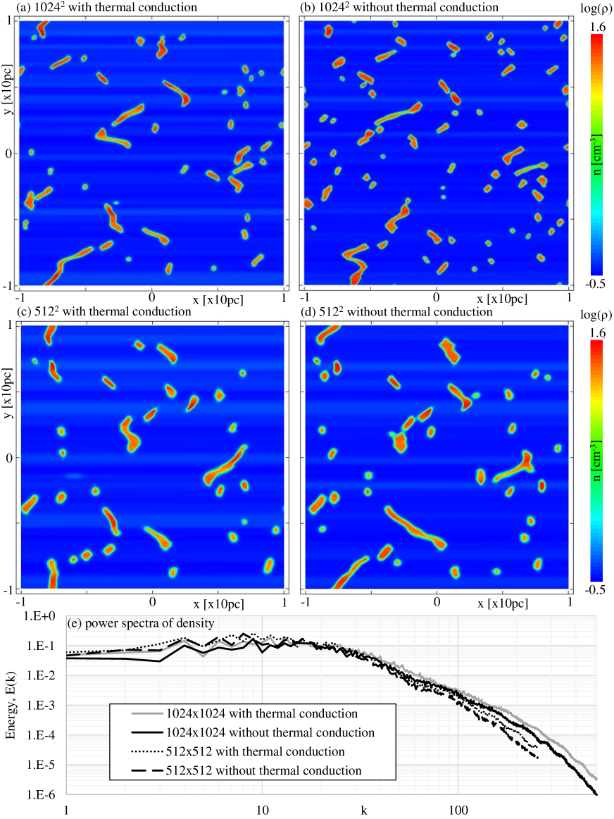
Figure 12: A comparison of simulations with and without thermal conduction and at different resolutions, as discussed in the text. Raw data are available from https://doi.org/10.5518/897.

Fig. 12 shows a comparison between calculations with and without conduction. These are two dimensional calculations with periodic boundary conditions with random initial conditions as described in Section 2. These initial conditions were imposed on the fully refined $512^{2}$ grid and projected onto the fully refined $1024^{2}$ grid, thereby ensuring the same wavelengths are present on both grids. This is as close as we can get to the same initial conditions for both resolutions. The alternative of imposing the initial conditions on the 1024² grid and projecting to 512² is less satisfactory since it introduces wavelengths on the $1024^{2}$ grid which cannot be represented on the $512^{2}$ grid. At the unperturbed initial density, $n=1.1$, equation (4) gives $\lambda_{F}=0.564$ pc. There are therefore approximately $14$ and $29$ cells in the initial Field length at the low and high resolutions, which is an adequate representation of the Field scale. Note that equation (5) gives $\lambda_{F}=0.0587$ pc.

It can be seen that these calculations all give very similar results and are much the same as the two dimensional calculations in Wareing et al. (2016) which had a much larger mesh spacing of $0.156$ pc. The main difference is that thermal conduction reduces the number of small clouds, which is to be expected and agrees with Hennebelle & Audit (2007) who found that the mass distribution of the larger clouds is not much affected by thermal conduction. In our calculations there is a collapse to a corrugated sheet, during which such small clouds are mostly absorbed by the larger ones. It should be noted that whilst there are slight differences between the power spectra at large and small-scales, they are all converged at intermediate wavenumbers, $k=11-40$, further increasing confidence in the thermal structure that forms at these size-scales. The factor of 4 difference which is apparent at the smallest scales (though inverted and less at the largest scales) is not down to differences in the initial condition. This could be down to slight differences in growth rates at the finest cell sizes.

Other authors have found similar results e.g. Piontek & Ostriker (2004) used a larger value of the thermal conductivity than (6) but argue that this does not have much effect on the final properties of the larger clouds. Gazol & Vázquez-Semadini (2002) did not include thermal conduction in their simulations with driven turbulence, but they also found that the small scale structure did not have a significant effect on the global properties. Inoue & Omukai (2015) included thermal conduction, but were not able to resolve the Field length in their large scale calculations. However, they also found that the properties of the thermally bistable medium converged on large scales, because “most of the mass of the cold gas created by thermal instability is contained in large clumps that are formed by the growth of large-scale fluctuations.”

AMR cannot be used for the initial evolution of the instability since it would derefine unless the error tolerance is very small. This makes it impossible to resolve the Field length in large scale calculations such as these since the minimum Field length is $0.0485$ pc at $n=6.2517$ (note that the Field length is only meaningful in the unstable region). It is therefore fortunate that the final distribution of large clouds is insensitive to the value of the thermal conductivity.

References

- André et al. (2014) André P., Di Francesco J., Ward-Thompson D., Inutsuka S.-i., Pudritz R. E., Pineda J. E., 2014, in Beuther H., Klessen R. S., Dullemond C. P., Henning T., eds, Protostars and Planets VI. University of Arizona Press, Tucson, 914. p. 27, preprint (arXiv:1312.6232)
- Bally et al. (1987) Bally J., Langer W. D., Stark A. A., Wilson R. W., 1987, ApJ, 312, L45
- Bergin & Tafalla (2007) Bergin E. A., Tafalla M., 2007, ARAA, 45, 339
- Berry (2015) Berry D. S., 2015, Astronomy and Computing, 10, 22
- Coudé et al. (2019) Coudé S., et al. 2019, ApJ, 877, article id. 88
- Cox et al. (2016) Cox N. L. J., et al. 2016, A&A, 590, id.A110
- Crutcher et al. (2010) Crutcher R. M., Wandelt B., Heiles C., Falgarone E., Troland T. H., 2010. ApJ, 725, 466
- Crutcher (2012) Crutcher R. M., 2012, ARAA, 50, 29
- Doi et al. (2020) Doi Y., et al. 2020, ApJ, 899, id.28
- Falle (1991) Falle S. A. E. G., 1991, MNRAS, 250, 581
- Falle et al. (2020) Falle S. A. E. G., Wareing C. J., Pittard J. M., 2020, MNRAS, 492, 4484
- Fissel et al. (2019) Fissel L. M., et al., 2019, ApJ, 878, 110
- Field (1965) Field G. B., 1965, ApJ, 142, 531
- Gazol & Vázquez-Semadini (2002) Gazol A., Vázquez-Semadini E., 2005, ApJ, 630, 911
- Gent et al. (2013) Gent F. A., Shukurov A., Fletcher A., Sarson G. R., Mantere M. J., 2013, MNRAS, 432, 1396
- Girart et al. (2009) Girart J. M., Beltrán M. T., Zhang Q., Rao R., Estalella R., 2009, Science, 324, 1408
- Girichidis et al. (2018) Girichidis P., Seifried D., Naab T., Peters T., Walch S., Wünsch R., Glover S. C. O., Klessen R. S., 2018, MNRAS, 480, 3511
- Goldsmith et al. (2008) Goldsmith P. F., Heyer M., Haraynan G., Snell R., Li D., Brunt C., 2008, ApJ, 680, 428
- Hennebelle & Audit (2007) Hennebelle P., Audit E., 2007, A&A, 465, 431
- Hennebelle et al. (2007) Hennebelle P., Audit E., Miville-Deschênes M.-A., 2007, A&A, 465, 445
- Hennebelle & Inutsuka (2019) Hennebelle P., Inutsuka S.-i., 2019, Front. Astron. Space Sci., 6, 5
- Hull & Zhang (2019) Hull C. L. M., Zhang Q., 2019, Front. Astron. Space Sci., 6, 3
- Inoue & Omukai (2015) Inoue T., Omukai K., 2015, ApJ, 805, 73
- Kandori et al. (2017) Kandori R., Tamura M., Kusakabe N., Nakajima Y., Kwon J., Nagayama T., Nagata T., Tomisaka K., Tatematsu K., 2017, ApJ, 845, 32
- Kandori et al. (2018) Kandori R., et al. 2018, ApJ, 865, 121
- Kong et al. (2018) Kong S., et al. 2018, ApJS, 236, 25
- Kowal et al. (2007) Kowal G., Lazarian A., Beresnyak A., 2007, ApJ, 658, 423
- Koyama & Inutsuka (2002) Koyama H., Inutsuka S.-i., 2002, ApJ, 564, L97
- Koyama & Inutsuka (2004) Koyama H., Inutsuka S.-i., 2004, ApJL, 602, L25
- Krumholz & Burkhart (2016) Krumholz M. R., Burkhart B., 2016, MNRAS, 458, 1671
- Krumholz & Federrath (2019) Krumholz M. R., Federrath C., 2019, Front. Astron. Space Sci., 6, 7
- Li et al. (2013) Li H.-b., Fang M., Henning T., Kainulainen J., 2013, MNRAS, 436, 3707
- Li et al. (2015) Li P. S., McKee C. F., Klein R. I., 2015, MNRAS, 452, 2500
- Liu et al. (2019) Liu H.-L., Stutz A., Yuan J.-H., 2019, MNRAS, 487, 1259
- Liu et al. (2019b) Liu J., et al. 2019, ApJ, 877, article id. 43
- González Lobos & Stutz (2019) González Lobos V., Stutz A., 2019, MNRAS, 489, 4771
- Loren (1989) Loren R. B., 1989, ApJ, 338, 925
- Malinen et al. (2016) Malinen J., et al. 2016, MNRAS, 460, 1934
- Medina et al. (2014) Medina S.-N. X., Arthur S. J., Henney W. J., Mellema G., Gazol A., 2014, MNRAS, 445, 1797
- Mouschovias (1976a) Mouschovias T. C., 1976a, ApJ, 206, 753
- Mouschovias (1976b) Mouschovias T. C., 1976b, ApJ, 207, 141
- Mouschovias & Spitzer (1976) Mouschovias T. C., Spitzer L. Jr, 1976, ApJ, 210, 326
- Ntormousi & Hennebelle (2019) Ntormousi E., Hennebelle P., 2019, A&A, 625, A82
- Padoan et al. (2006) Padoan P., Juvela M., Kritsuk A., Norman M. L., 2006, ApJ, 653, L125
- Palmeirim et al. (2013) Palmeirim P., et al. 2013, A&A, 550, id.A38
- Panopoulou et al. (2015) Panopoulou G., et al. 2015, MNRAS, 452, 715
- Parker (1953) Parker E. N., 1953, ApJ, 117, 431
- Pattle et al. (2017) Pattle K., et al. 2017, ApJ, 846, article id. 122
- Pattle & Fissel (2019) Pattle K., Fissel L., 2019, Front. Astron. Space Sci., 6, 15
- Piontek & Ostriker (2004) Piontek R. A., Ostriker E. C., 2004, ApJ, 601, 905
- Schleuning (1998) Schleuning D. A., 1998, ApJ, 493, 811
- Shimajiri et al. (2019) Shimajiri Y., Andre Ph., Palmeirim P., Arzoumanian D., Bracco A., Könyves V., Ntormousi E., Ladjelate B., 2019, A&A, 623, A16
- Soam et al. (2018) Soam A., et al. 2018, ApJ, 865:61
- Stutz & Gould (2016) Stutz A., Gould A., 2016, A&A, 590, A2
- Stutz et al. (2018) Stutz A., Gonzalez-Lobos V. I., Gould A., MNRAS submitted. arXiv:1807.11496
- Teyssier & Commerçon (2019) Teyssier R., Commerçon B., 2019, Front. Astron. Space Sci., 6, 51
- Tritsis et al. (2015) Tritsis A., Panopoulou G. V., Mouschovias T. Ch., Tassis K., Pavlidou V., 2015, MNRAS, 451, 4384
- Tritsis & Tassis (2016) Tritsis A., Tassis K., 2016, MNRAS, 462, 3602
- Tritsis & Tassis (2018) Tritsis A., Tassis K., 2018, Science, 360, 6389, 635