Information transfer between turbulent boundary layer and porous media

Abstract

The interaction between the flow above and below a permeable wall is a central topic in the study of porous media. While previous investigations have provided compelling evidence of the strong coupling between the two regions, few studies have quantitatively measured the directionality, i.e., causal-and-effect relations, of this interaction. To shed light on the problem, we use transfer entropy as a marker to evaluate the causal interaction between the free turbulent flow and the porous media using interface-resolved direct numerical simulation. Our results show that the porosity of the porous medium has a profound impact on the intensity, time scale and spatial extent of surface-subsurface interactions. For values of porosity equal to 0.5, top-down and bottom-up interactions strongly are asymmetric, the former being mostly influenced by small near-wall eddies. As the porosity increases, both top-down and bottom-up interactions are dominated by shear-flow instabilities.

1 Introduction

Turbulent shear flows over porous walls are frequently encountered in the natural environment and industrial applications, such as oil wells, catalytic reactors, heat exchangers, and porous river beds, to name a few. As the blocking effect of the wall is relaxed, the porous bed allows for mass, momentum and energy exchange across the permeable interface, which triggers changes in both the surface and subsurface flows (Breugem et al., 2006; Manes et al., 2011; Kim et al., 2020; Fang et al., 2018; Suga et al., 2020). A widely observed form of interaction in flows over porous beds is the upwelling and downwelling motion across the permeable interface, which enables the exchange of information between surface and subsurface flow. Studies relying on correlation analysis, conditional averaging, and modal analysis have revealed that the transport of wall-normal fluid across the interface is accompanied by streamwise velocity fluctuations in surface flow (Breugem et al., 2006; Kim et al., 2020). Moreover, the turbulence intensity below the interface is also modulated by outer large-scale motions Efstathiou & Luhar (2018); Kim et al. (2020). The influence of the porous bed is not constrained to the near-wall region. It has been observed that large-scale vortical structures emerge in the surface flow as the wall permeability increases, which has been attributed to Kelvin-Helmholtz (KH) type of instabilities from inflection points of the mean velocity profile (Jiménez et al., 2001; Breugem et al., 2006; Manes et al., 2011). In addition, the streaks and streamwise vortices characteristic of the near-wall cycle are substantially weakened in the presence of porous walls compared to smooth-wall turbulence. This suggest that the flow structure over porous walls is is governed by the balance of two competing mechanism: the formation of wall-attached eddies and the disruption by shear layer instabilities Manes et al. (2011); Efstathiou & Luhar (2018).

Despite the last advancements in the field, the dynamics of the mass and momentum transfer across the interface of porous media is far from being settled. Although we do have a solid knowledge on the flow structures resulting from the surface-subsurface interaction, the fundamental cause-effect relations of these fluid motions are rarely inspected. To what extent does the outer turbulence determines the flow inside porous media and vice versa? These questions cannot be addressed by correlation analysis and traditional mode decomposition methods (e.g. proper orthogonal decomposition, POD) as these approaches do not provide the directionality and time asymmetry required to quantify causation (Kantz & Schreiber, 2004; Pearl, 2009). Recently, Lozano-Durán et al. (2020a) highlighted the importance of causal inference in fluid mechanics (see also Lozano-Durán et al., 2020b) and proposed to leverage information theoretic metrics to explore causality in turbulent flows. In particular, Lozano-Durán et al. (2020a) examined the causal interactions of energy-eddies in wall-bounded turbulence using transfer entropy (Schreiber, 2000). In this study, we conduct direct numerical simulation (DNS) of a fully-resolved interface and porous domain and follow the analysis of Lozano-Durán et al. (2020a) to quantify the causality among the interaction of surface and subsurface flow.

The work is organised as follows: we present the details of the DNS dataset and the definition of transfer entropy in §2. In §3, we discuss the typical upwelling/downwelling process and showed that the porosity of the media has a major impact on the inner and outer flow structures as well as in their causal relations. Finally, conclusions are offered in §4.

2 Numerical simulations and methods

2.1 Numerical setup

The three-dimensional incompressible Navier$-$Stokes equations are solved in non-dimensional form,

$$\frac{\partial u_{j}}{\partial x_{j}}=0,\quad\frac{\partial u_{i}}{\partial t}+\frac{\partial u_{i}u_{j}}{\partial x_{j}}=-\frac{\partial p}{\partial x_{i}}+\frac{1}{Re}\frac{\partial^{2}u_{i}}{\partial x_{j}\partial x_{j}}+\Pi\delta_{i1},$$ (1)

where $\Pi$ is a constant pressure gradient in the mean-flow direction. The governing equations are non-dimensionalized by normalizing lengths by half of distance between two cylinders $D/2$ (figure 1a), velocities by the averaged bulk velocity $U_{b}$ of the free flow region ($y=[0,10]$), such that time is non-dimensionalized by $D/(2U_{b}$). The spectral/$hp$ element solver Nektar++ (Cantwell et al., 2011) is used to discretize the numerical domain containing complex geometrical structures. The solver allows for arbitrary-order spectral/$hp$ discretisations with hybrid shaped elements. The time-stepping is performed with a second-order mixed implicit-explicit (IMEX) scheme. The time step is fixed to $\Delta T/(D/2U_{b})=0.005$.

Hereafter, the velocity components in the streamwise $x$, wall normal $y$ and spanwise $z$ directions are denoted as $u$, $v$ and $w$, respectively. The domain size ($L_{x}\times L_{y}\times L_{z}$) is $100\times 20\times 8\pi$. The lower half $y=[-10,0]$ contains the porous media and the upper half $y=[0,10]$ is the free channel-flow. The porous layer consists of 50 cylinder elements aligned along the streamwise direction and arranged in 5 rows in the wall-normal direction as illustrated in figure 1(a). The distance between two cylinders is fixed at $D=2$.

The no-slip boundary condition is applied to the cylinders, the upper wall, and lower wall. Periodic boundary conditions are used in streamwise and spanwise directions. The geometry is discretised using quadrilateral elements on the $x-y$ plane with local refinement near the interface. High-order Lagrange polynomials ($P=4-7$) are used within each element on the $x-y$ plane. The spanwise direction is extended with a Fourier-based spectral method.

Three DNS cases are performed with varying porosity $\varphi$, which is defined as the ratio of the void volume to the total volume of the porous structure. The parameters of simulations are listed in table 1. The superscripts $(\cdot)^{\mathrm{p}}$ and $(\cdot)^{\mathrm{t}}$ represent variables of permeable wall and top smooth wall sides, respectively. Variables with superscript $+$ are scaled by friction velocities $u_{\tau}$ of their respective side and viscosity $\nu$. The Reynolds number of top wall boundary layer is set to be $Re_{\tau}^{\mathrm{t}}=\delta^{\mathrm{t}}u_{\tau}^{\mathrm{t}}/\nu\approx 180$ for all cases ($\delta$ is the distance between the position of maximum streamwise velocity and the wall). In this manner, changes in the top wall boundary layer are minimized. On the top smooth wall side, the streamwise cell size ranges from $6.3\leq\Delta x^{\mathrm{t}+}\leq 8.5$ and the spanwise cell size is below $\Delta z^{\mathrm{t}+}=5.6$. On the porous media side, $\Delta z^{\mathrm{p}+}$ is below 8.4, whereas $\Delta x^{\mathrm{p}+}$ and $\Delta y^{\mathrm{p}+}$ are enhanced by polynomial refinement of local mesh (Cantwell et al., 2011).

case	$\varphi$	$U_{b}$	$u_{\tau}^{\mathrm{p}}$	$Re_{\tau}^{\mathrm{p}}$	$\Delta x^{\mathrm{p}+}$/$\Delta y^{\mathrm{p}+}$/$\Delta z^{\mathrm{p}+}$	$u_{\tau}^{\mathrm{t}}$	$Re_{\tau}^{\mathrm{t}}$	$\Delta x^{\mathrm{t}+}$/$\Delta y^{\mathrm{t}+}$/$\Delta z^{\mathrm{t}+}$
C05	0.50	4.1	0.31	336	2.2/0.38/5.3	0.27	180	6.3/0.43/4.5
C06	0.60	4.1	0.36	464	3.5/0.50/6.8	0.28	190	5.5/0.47/ 5.4
C07	0.70	4.0	0.38	625	4.2/0.55/8.4	0.23	160	5.2/0.51/ 5.1
C08	0.80	3.0	0.38	793	4.3/0.64/8.0	0.21	170	8.5/0.34 /5.6

Table 1: Simulation parameters. The porosity of the porous medium region is $\varphi$. The friction Reynolds numbers for the porous and impermeable top walls are $Re_{\tau}^{\mathrm{p}}$ and $Re_{\tau}^{\mathrm{t}}$, respectively. $\Delta x^{\mathrm{p}+}$/$\Delta y^{\mathrm{p}+}$/$\Delta z^{\mathrm{p}+}$ and $\Delta x^{\mathrm{t}+}$/$\Delta y^{\mathrm{t}+}$/$\Delta z^{\mathrm{t}+}$ are the respective grid spacings in wall units of porous wall and top wall, respectively.

2.2 Causality among time signals as transfer entropy

We use transfer entropy (Schreiber, 2000) as a marker to evaluate the direction of coupling, i.e., the cause-effect relationship, between two time-signals representative of some fluid quantities of interest (Lozano-Durán et al., 2020a). Transfer entropy is an information-theoretic metric representing the dependence of the present of $X$ on the past of $Y$. This dependence is measured as the decrease in uncertainty (or entropy) of the signal $X$ by knowing the past state of $Y$. Transfer entropy from $X$ and $Y$ is formally defined as

$$T_{Y\rightarrow X}(\Delta t)=H(X_{t}|X_{t-1})-H(X_{t}|{X_{t-1},Y_{t-\Delta t}}),$$ (2)

where the subscript $t$ denotes time and $\Delta t$ is the time-lag to evaluate causality. $H(A|B)$ is the conditional Shannon entropy of the variable $A$ given $B$,

$$H(A|B)=E[\mathrm{log}(p(A,B))]-E[\mathrm{log}(p(B))],$$ (3)

where $p(\cdot)$ is the probability density function, and $E[\cdot]$ denotes the expected value.

In order to quantify the relative strength of causality, we scale the magnitude of $T_{Y\rightarrow X}$ within the range $[0,1]$ and define the normalized transfer entropy (Gourévitch & Eggermont, 2007),

$$\tilde{T}_{Y\rightarrow X}=\frac{T_{Y\rightarrow X}-E[T_{Y^{s}\rightarrow X}]}{H(X_{t}|X_{t-1})},$$ (4)

where $H(X_{t}|X_{t-1})$ is the intrinsic uncertainty of $X$ conditioned on knowing its own history. Thus, (4) represents the fraction of information in $X$ not explained by its own past that is explained by the past of $Y$. The term $E[T_{Y^{s}\rightarrow X}]$ is introduced to alleviate the bias due to statistical errors. This is achieved with the surrogate variable $Y^{s}$, which is constructed by randomly permuting $Y$ in time to break any causal links with $X$.

3 Results

3.1 Mean velocity and turbulent kinetic energy profiles

The mean statistics of the three cases are briefly discussed here to outline the impact of porosity on surface and subsurface flow. Figure 1(b,c) shows the mean profiles for the streamwise velocity $\langle\overline{u}\rangle$ and turbulent kinetic energy (TKE) $\langle\overline{q}\rangle=\langle\overline{u^{\prime}u^{\prime}+v^{\prime}v^{\prime}+w^{\prime}w^{\prime}}\rangle/2$ normalized by $u_{\tau}^{t}$. The operators $\langle\cdot\rangle$ and $\overline{(\cdot)}$ represent spatial average in $x$-$z$ and temporal average, respectively, and the superscript prime denotes turbulent fluctuations $\phi^{\prime}=\phi-\overline{\phi}$. The profiles of impermeable smooth wall channel from Hoyas & Jiménez (2008) are also included for comparison. For increasing wall porosity, the mean velocity profile becomes more skewed toward the top wall as a consequence of the higher skin friction on the porous wall Breugem et al. (2006). Below the interface ($y=0$), the mean velocity profiles exhibit a clear inflection point, which is typically associated with KH-type instabilities responsible for additional turbulent structures (Manes et al., 2011). This is partly substantiated by figure 1(c), which shows that the TKE below and above the interface is significantly enhanced for highest porosity considered here (case C08). In the following sections, we illustrate how the change of flow structures in the interface region affects the interaction between surface and sub-surface flow.

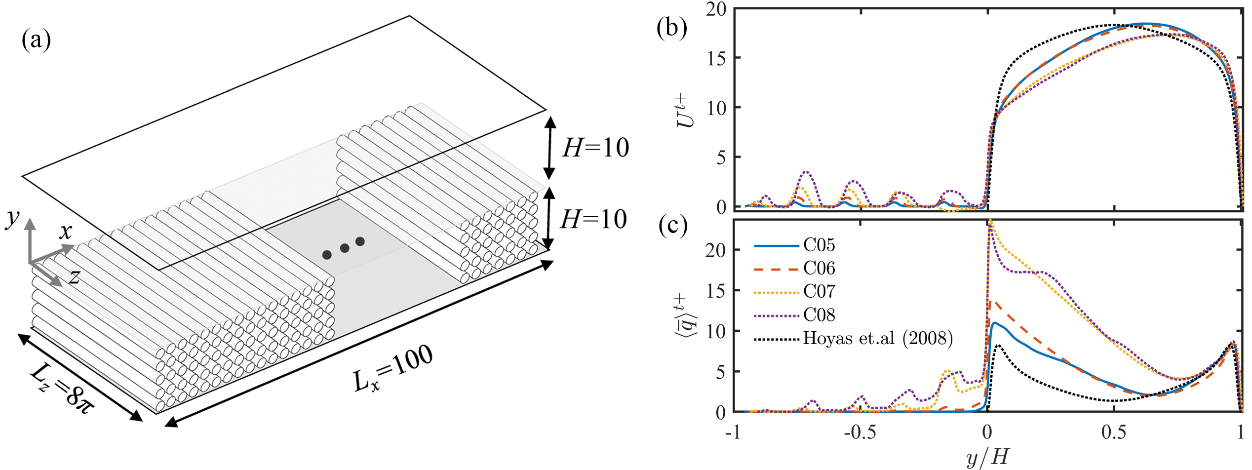
Figure 1: (a) Configuration of the computational domain; (b) mean streamwise velocity normalized by $u_{\tau}^{\mathrm{t}}$; (c) mean TKE profiles normalized by $u_{\tau}^{\mathrm{t}2}$. Profiles of impermeable smooth wall channel (Hoyas & Jiménez (2008), $Re_{\tau}=180$) are superimposed in (b,c) for comparison.

3.2 Upwelling and downwelling events

The upwelling/downwelling events transport fluid directly across the interface, which provide an intuitive picture of the interaction process. Examples of typical upwelling and downwelling events are captured in figure 2 for case C05. During the upwelling event (figure 2a, $x/D=1$), a small amount of fluid is ejected from beneath the interface ($t=0$), which later becomes a low speed bulb above the interface ($t=0.15$-$0.3$) to finally merged with a large low-speed structure downstream ($t=0.45$). During the downwelling event (figure 2b, $x/D=1$), a portion of low-speed fluid is absorbed into the porous medium ($t=0$). The low-speed structure is later separated into two structures as the upper part is convected downstream ($t=0.15$-$0.45$). The observations from the instantaneous fields also suggest that upwelling/downwelling events are subjected to the modulation of large-scale motions in free flow region. Specifically, the upwelling events at the gaps are often related to large-scale low-speed structures above the interface (see figure 2a at $y/D=0.5$), while downwelling events are usually associated with high speed structures (see figure 2b at $y/D=0.5$). This connection was also observed by Kim et al. (2018), and it is further discussed in the following sections. In addition, the momentum flux between neighbouring gaps is usually negatively correlated, i.e., upwelling and downwelling events usually occur side by side probably due to the constrain imposed by continuity at the interface.

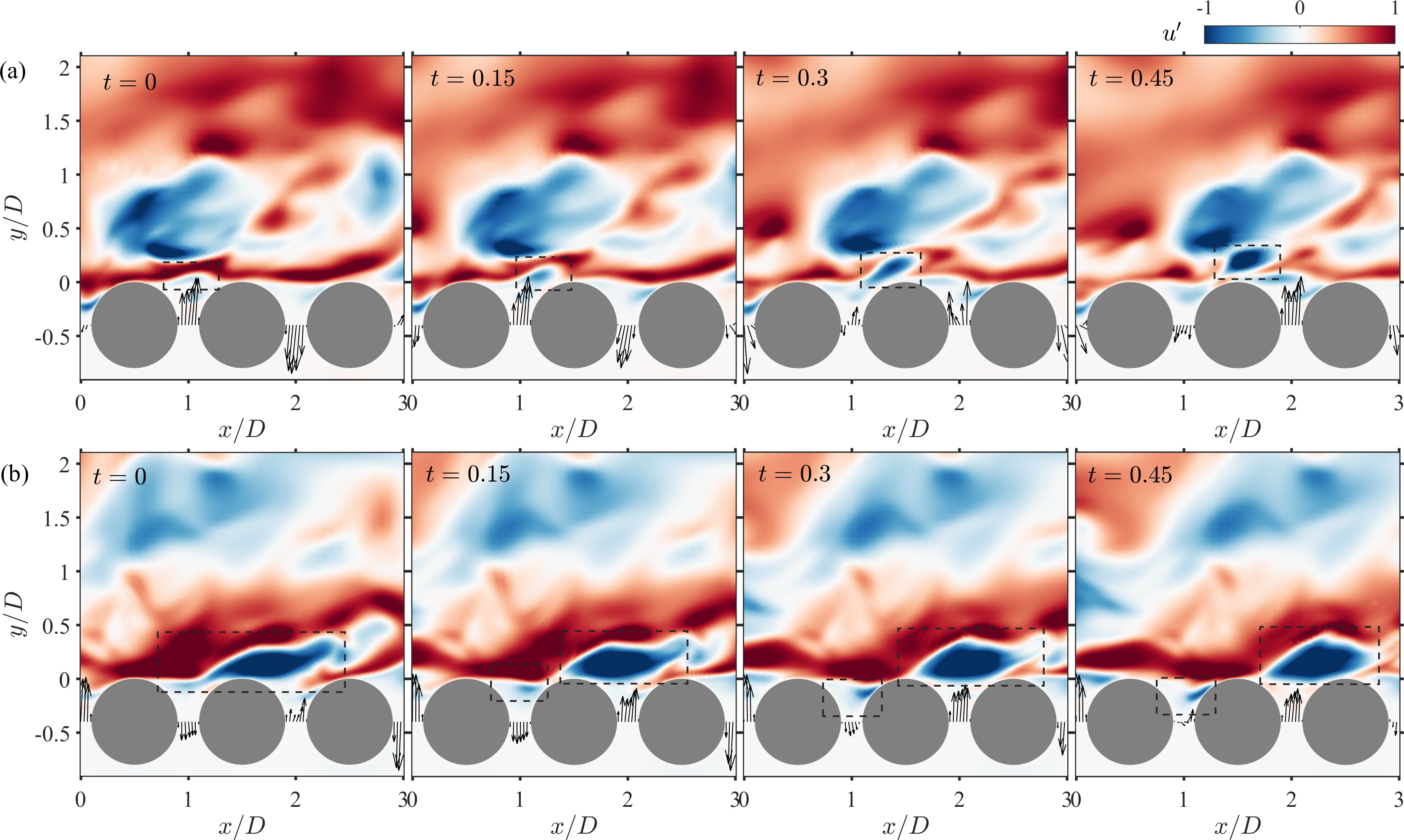
Figure 2: Instantaneous $u^{\prime}$ fields (C05) during (a) an upwelling event and (b) a downwelling event. Instantaneous $(u^{\prime},v^{\prime})$ at the gap between cylinders are illustrated by vectors.

3.3 Coherent structure of POD modes

To investigate the causal relation between surface and subsurface flows, we characterize the flow structure within each region using Proper Orthogonal Decomposition (POD). We extract energetic modes above and below the interface and use the corresponding time coefficients to measure causality between interactions. In POD, the fluctuating velocity field $\bm{u}^{\prime}(\bm{x},t)=[u^{\prime}(\bm{x},t),v^{\prime}(\bm{x},t),w^{\prime}(\bm{x},t)]$, is decomposed via optimal energy criteria into

$$\bm{u}^{\prime}\left({\bm{x},t}\right)=\sum\limits_{k=1}^{K}{{a_{k}}\left(t\right){\bm{\phi}_{k}}\left(\bm{x}\right)},$$ (5)

where $a_{k}(t)$ is the time coefficient for the $k^{\mathrm{th}}$ rank mode and $\bm{\phi}_{k}(\bm{x})$ are the modes which constitute an orthogonal spatial basis. We focus on the local information transfer in the vicinity of one pore unit. Consistently, the wall-normal extent of boundary layer region is selected from the crest height ($y=0$) to the channel center. For the porous medium region, we focus on the 1st layer of cylinders to capture the so called transition layer (Kim et al., 2020), i.e., the region with direct mass and momentum exchange with the free flow. The first modes for cases C05 and C08, denoted by $\phi^{\mathrm{p}}_{1}$ and $\phi^{\mathrm{t}}_{1}$, respectively (superscript p for ‘porous’ and t for ‘turbulent boundary layer’ or TBL), are shown in figure 3. The POD is computed from a time-series of of 2000 snapshots spanning a time of $TU_{b}/D=150$-$200$. The time interval between snapshot is chosen to be $\Delta tU_{b}/D\approx 0.1$, which is $\mathcal{O}(10^{-2})$ the time scale of the typical period of fluctuations inside porous media (discussed later in figure 3d). The PODs are computed for all 50 pore units in streamwise and 12 evenly-spaced positions in spanwise direction (spanwise interval $\Delta Z^{\mathrm{t}+}\geq 100$). The consistency of POD modes at different positions is checked by evaluating the correlation coefficients between the $\phi^{\mathrm{p}}_{1}$ (or $\phi^{\mathrm{t}}_{1}$) at different $x$ and $z$ positions, which are at a high level of $0.97\pm 0.02$.

For the two porosities shown in figure 3, the 1st mode for the TBL region $\phi^{\mathrm{t}}_{1}$ consists of a large countergradient region (i.e., Q2 when $u^{\prime}<0$ and $v^{\prime}>0$, and Q4 when $u^{\prime}<0$ and $v^{\prime}>0$). Although the streamwise extent of this structure is unknown due to the limited field of view, the wall-normal extent reaches the center of the channel and hence it can be deemed as ‘large’. The 1st mode in the porous region $\phi^{\mathrm{p}}$ shows a richer structure which is dramatically affected by the porosity. In case C05, $\phi^{\mathrm{p}}_{1}$ encompasses a vortex trapped on the top of the cylinder’s gap, and a vertical momentum transfer within the gap. In contrast, the vortex above the gap is considerably smaller in C08, leaving room for a stronger vertical momentum flux within the gap. Figure 3(c) shows that the modes $\phi^{\mathrm{p}}_{1}$ already account for 40-50% of the TKE and they are taken as the simplest representation of the flow patterns close to the interface.

The time coefficients of first modes, $a^{\mathrm{t}}_{1}$ and $a^{\mathrm{p}}_{1}$, are compared in figure 3(d). Note that time coefficients represent the instantaneous magnitude of corresponding spatial mode and, as such, can be used as markers of the flow structure in each region. In the current context, $a^{\mathrm{t}}_{1}$ denotes the intensity of Q2/Q4 events above the pore unit, whereas $a^{\mathrm{p}}_{1}$ reflects the strength of the vortex and momentum flux at the gap. An excerpt of the time series of $a^{\mathrm{t}}_{1}$ and $a^{\mathrm{p}}_{1}$ is plotted in figure 3(d)-left. Overall, both time-signals show a certain degree of synchronization, which seems to become stronger as porosity increases. Large-scale fluctuations with period $\Delta TU_{b}/D\geq 10$ can be observed in $a^{\mathrm{t}}_{1}$ and $a^{\mathrm{p}}_{1}$ for low porosity case C08, the scale of which is consistent with the prediction of linear stability theory Jiménez et al. (2001) and experimental observations Manes et al. (2011); Kim et al. (2020). Figure 3(d)-right contains the joint probability density function (JPDF) of $a^{\mathrm{t}}_{1}$ and $a^{\mathrm{p}}_{1}$ and shows that the mode is distributed along $a^{\mathrm{t}}_{1}\sim a^{\mathrm{p}}_{1}$ for both case C08 and case C05, with the variables in the former case being clearly more correlated. However, the JPDF does not provides information about the direction of interaction, i.e., whether $a^{\mathrm{t}}_{1}$ causes $a^{\mathrm{p}}_{1}$ or vice versa.

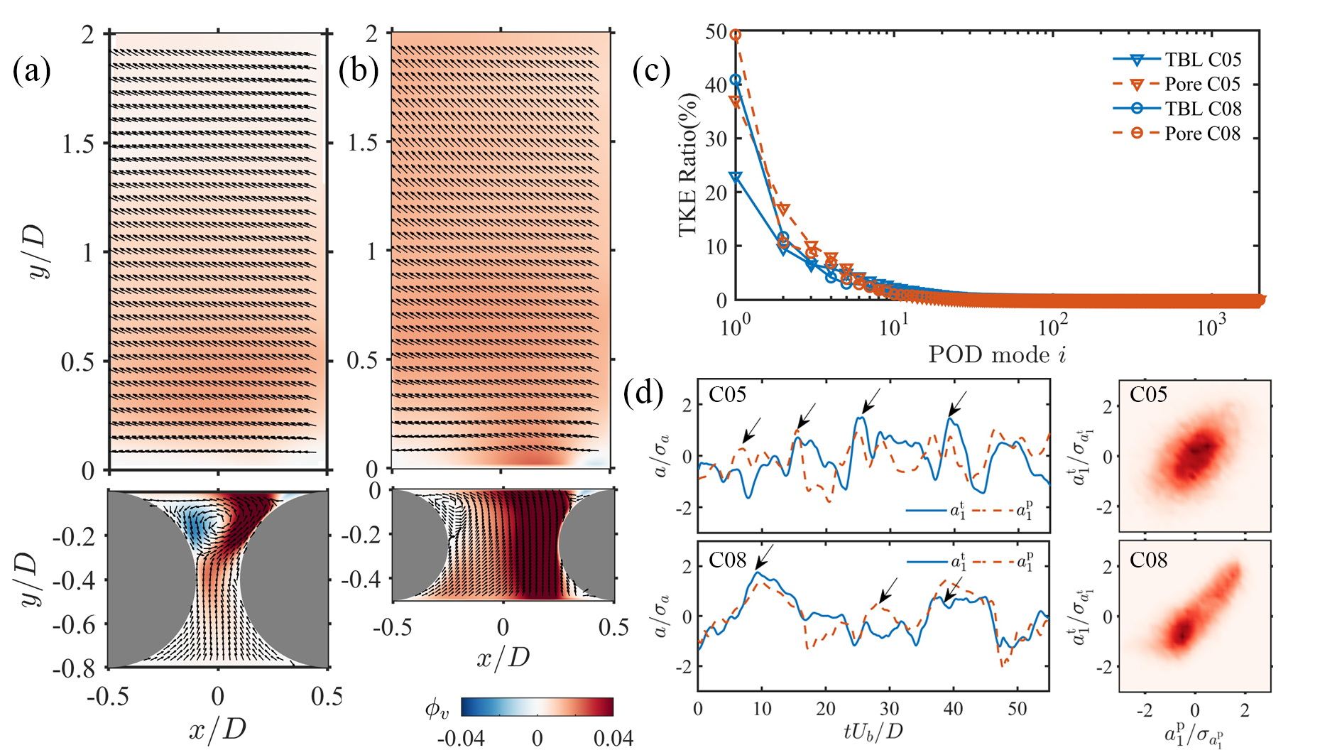
Figure 3: First POD spatial mode of TBL $\phi^{\mathrm{t}}_{1}$ and porous region $\phi^{\mathrm{p}}_{1}$ for cases (a) C05 and (b) C08; (c) shows the TKE contribution ratio of mode order $i$;(d) shows the time coefficient $a^{\mathrm{t}}_{1}$ (blue solid line) and $a^{\mathrm{p}}_{1}$ (red dashed line) as well as their joint PDF for cases C05 (upper row) and C08 (lower row).

3.4 Information transfer between free-flow and porous-media structures

We assess the causal relation between the coherent structures by evaluating the transfer entropy between $a^{\mathrm{t}}_{1}$ and $a^{\mathrm{p}}_{1}$. The contour of normalized transfer entropy of the time coefficients is shown in figure 4 as a function of time-delay $\Delta t$ (i.e., the time-horizon for causality as shown in figure (2)). The information transfer between different pore units is also inspected, with $l$ the streamwise offset of target time coefficient $X=a^{\mathrm{t}}_{1,l}(t)$ (or $a^{\mathrm{p}}_{1,l}(t)$) from $Y=a^{\mathrm{p}}_{1}(t)$ (or $a^{\mathrm{t}}_{1}(t)$). For example, $l/D=2$ denotes a target signal $X$ acquired 2 pore units downstream the location of $Y$. We take into account all 50 pore units in the streamwise direction and 12 spanwise positions, which amounts to a number of samples equal to $\mathcal{O}(10^{6})$ for each case. Adaptive binning method (Darbellay & Vajda, 1999) is used to estimate the probability density function in (2) with the bin number equal to 50 in each dimension according to the empirical recommendation of Hacine-Gharbi et al. (2012). It was tested that doubling and halving the number of bins did not alter the conclusions presented hereafter.

The strongest values of $\tilde{T}$ are organized along the two ridges in the space of $(l,\Delta t)$ indicated by solid and dashed lines in figure 4. These ridges mark the time delay and spatial offset at which information transfer between the two signals is maximum. When $X$ and $Y$ are within the same pore unit ($l=0$), the time lag to reach maximum $\tilde{T}_{a^{\mathrm{t}}_{1}\rightarrow a^{\mathrm{p}}_{1}}$ and $\tilde{T}_{a^{\mathrm{p}}_{1}\rightarrow a^{\mathrm{t}}_{1}}$ is $\Delta tU_{b}/D\approx 2$. This delay can be interpreted as the elapsed time of the fluid in porous media to the influence the free flow, or vice versa. For increasing $l$, the time delay for maximum transfer entropy increases linearly with $l$ along the upper ridge (solid lines) with a slope of $l/\Delta t\approx 0.4U_{b}$. This linear increase of the time delay can be explained by the convection of the turbulent structures from the position of source signal to the target signal at a mean speed of $0.4U_{b}$.

For $l\geq 1$, a second ridge appears in figure 4 (dashed lines). For $\tilde{T}_{a^{\mathrm{p}}_{1}\rightarrow a^{\mathrm{t}}_{1}}$, the information transfer along this second ridge is stronger than along the first ridge discussed above, suggesting that the ‘bottom-up’ coupling is stronger between neighbouring pore units. The emergence of the second ridge could be attributed to the linkage of neighbouring pore units. As shown in figure 2, a local upwelling/downwelling events are usually accompanied by a downwelling/upwelling event at nearby pore units, owing to the continuity constraint. This leads to a general phase shift between the fluctuations in neighbouring pore units and also a strong coupling effect between them. Such a coupling of neighbouring pore units make it possible for the the upstream sub-surface fluctuations to affect downstream free flow indirectly, which is reflected on the second ridge in figure 4(a2,b2).

Despite the similarities observed for different porosities, there are striking differences between the two cases shown in figure 4. The magnitude of $\tilde{T}$ as well as its time and spatial extent are larger for case C08 (i.e., larger porosity) than for case C05. The results might be explained by noting that, first, the gap of cylinders in C05 is covered by a strong vortex, which blocks the free flow from entering the porous medium region directly (as shown in figure 3a). On the other thand, the gap is free from any obstructing vortex for C08 (figure 3b), which facilitates the exchange of fluid. The larger time and spatial extent for high porosity cases can be attributed to the large scale KH eddies originated from the inflection of mean profile, which is further studied in the next section. The behavior of cases C06 and C07, omitted for brevity, is situated between C05 and C08.

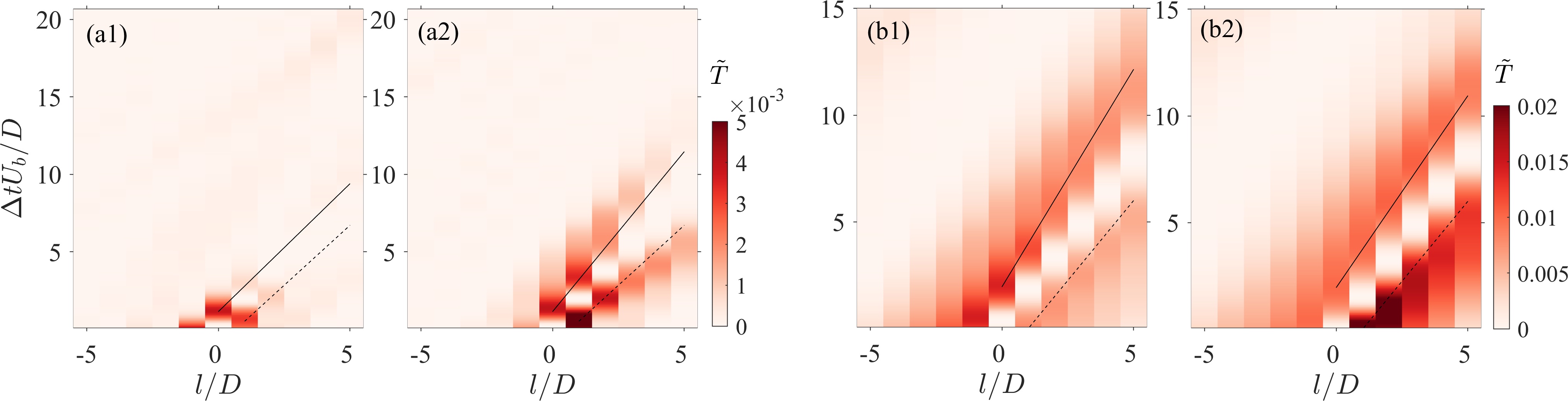
Figure 4: Transfer entropy of POD time-coefficients. Case C05: (a1) $\tilde{T}_{a^{\mathrm{t}}_{1}\rightarrow a^{\mathrm{p}}_{1}}$; (a2) $\tilde{T}_{a^{\mathrm{p}}_{1}\rightarrow a^{\mathrm{t}}_{1}}$. Case C08: (b1) $\tilde{T}_{a^{\mathrm{t}}_{1}\rightarrow a^{\mathrm{p}}_{1}}$; (b2) $\tilde{T}_{a^{\mathrm{p}}_{1}\rightarrow a^{\mathrm{t}}_{1}}$. Solid and dashed lines are used to mark the upper and lower ridges on the contours, respectively.

3.5 The dependence of causality on time scale

The fluctuations in the turbulent free flow consist of multiple time scales as illustrated by the POD time coefficients shown in figure 3(d). In this section, we investigate which of these scales have largest impact on the interactions between turbulent and sub-surface flow. To address this point, a band-pass filter is applied to $a^{\mathrm{t}}_{1}$ to select modes in a certain frequency range,

$$\check{a}^{\mathrm{t}}_{1}(t)=\int_{f_{c}-0.5B}^{f_{c}+0.5B}\hat{a}^{\mathrm{t}}_{1}(f)e^{2\pi\mathrm{i}ft}\mathrm{d}f+\int_{-f_{c}-0.5B}^{-f_{c}+0.5B}\hat{a}^{\mathrm{t}}_{1}(f)e^{2\pi\mathrm{i}ft}\mathrm{d}f$$ (6)

where $(\check{\cdot})$ indicates a band-pass filtered signal; $(\hat{\cdot})$ denotes the Fourier transformation in time; $f_{c}$ is the central frequency of the filter band and $B$ is the bandwidth. The bandwidth is set to $BD/U_{b}=0.1$, which provides a balance between localised frequencies and statistical convergence of the results. The transfer entropy as defined in (4) is then evaluated between $\check{a}^{\mathrm{t}}_{1}$ and $a^{\mathrm{p}}_{1}$. The results (colored contour in figure 5) reveal fundamental differences between top-down and bottom-up interactions as a function of porosity.

For case C05, the top-down information transfer $\tilde{T}_{\check{a}^{\mathrm{t}}_{1}\rightarrow a^{\mathrm{p}}_{1}}$ is mainly carried out by modes within the range $f_{c}D/U_{b}\approx 0.1$–$0.3$ (figure 5a1), which translates into a streamwise wavelength of $\lambda_{x}\approx U_{b}u_{\tau}^{\mathrm{p}}/(f_{c}\nu)\approx 300$–$1000$ in wall units using Taylor’s hypothesis. This is close to the length scale of near-wall streamwise vortices and streaks, suggesting that near-wall structures have a considerable impact on the momentum transport inside porous medium. On the other hand, bottom-up transfer $\tilde{T}_{a^{\mathrm{p}}_{1}\rightarrow\check{a}^{\mathrm{t}}_{1}}$ mostly resides on the low-frequency modes $f_{c}D/U_{b}\approx 0.02$–$0.05$ (figure 5a2), which suggests that the main effect of the sub-surface flow on the upper turbulent boundary layer is the disruption of large-scale structures by upwelling/downwelling events. This is consistent with figure 4 (a1,a2) where bottom-up information transfer persists for longer distances than top-down events.

The scale dependence in case C08 is notably different from case C05. In the former, low frequency modes ($f_{c}D/U_{b}<0.1$) dominate both top-down and bottom-up information transfer. The characteristic frequency of shear instability can be estimated for case C08 by the relation suggested by Ghisalberti & Nepf (2002) as $f_{\mathrm{KH}}D/U_{b}\approx 0.04$, which is consistent with the active large-scale modes in figure 5(b1,b2). Moreover, the time sequence of $a^{\mathrm{t}}_{1}$ and $a^{\mathrm{p}}_{1}$ in figure 3(d) also hints at low frequency fluctuations close to $f_{\mathrm{KH}}$. These observations suggest that the near wall turbulence in case C08 is dominated by large-scale shear instability modes, which give rise to strong surface-subsurface interactions. The presence of KH eddies in C08 overwhelms the role of near-wall attached eddies and demonstrates that the change of wall permeability can fundamentally altered the interaction scheme. The cases with medium porosity C06 and C07 exhibit a behavior closer to C08 in terms of scale dependency, and they are not shown here for the sake of brevity.

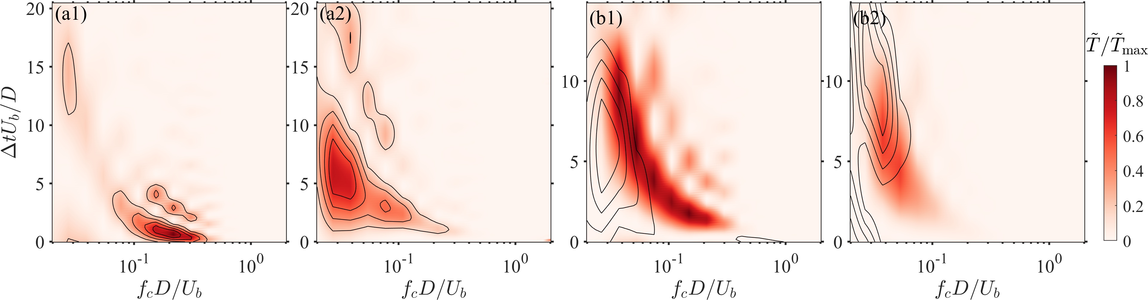
Figure 5: Dependence of transfer entropy on time scale for (a1,a2) case C05 and (b1,b2) case C08. (a1,b1) colored contour: $\tilde{T}_{\check{a}^{\mathrm{t}}_{1}\rightarrow a^{\mathrm{p}}_{1}}$, isolines: $\tilde{T}_{\check{u}^{\mathrm{t}}\rightarrow M^{\mathrm{p}}}$ ; (a2,b2) colored contour: $\tilde{T}_{a^{\mathrm{p}}_{1}\rightarrow\check{a}^{\mathrm{t}}_{1}}$, isolines: $\tilde{T}_{M^{\mathrm{p}}\rightarrow\check{u}^{\mathrm{t}}}$. The levels of isolines are from 0.2 to 0.8 with a step of 0.2.

The POD time coefficients $a^{\mathrm{t}}_{1}$ and $a^{\mathrm{p}}_{1}$ used in the analysis above may lack information on very high-frequency fluctuations. For completeness, we assess the influence on the results of using signals with additional temporal spectral content. For the free flow region, we define the instantaneous turbulent fluctuation $u^{\mathrm{t}}=u^{\prime}(x_{c},y_{\mathrm{peak}},z_{c},t)$ from the peak of $\langle\overline{q}\rangle(y)$ ( $y_{\mathrm{peak}}^{+}\approx 15$) above the gap center $(x_{c},y_{c},z_{c})$. The instantaneous vertical mass flux across cylinder gaps $M^{\mathrm{p}}(t)=\int_{\mathrm{gap}}v^{\prime}(x,t)\mathrm{d}x$ is used to represent the temporal fluctuation in porous region caused by upwelling/downwelling events. The transfer entropy between band-pass filtered $\check{u}^{\mathrm{t}}$ and $M^{\mathrm{p}}$, $T_{\check{u}^{\mathrm{t}}\rightarrow M^{\mathrm{p}}}$ and $T_{M^{\mathrm{p}}\rightarrow\check{u}^{\mathrm{t}}}$, is then calculated following the same procedure as above, and the results are superimposed in figure 5 as solid isolines. For case C05, the result for the two sets of signals is essentially identical. For case C08, the patterns of $T_{\check{u}^{\mathrm{t}}\rightarrow M^{\mathrm{p}}}$ and $T_{M^{\mathrm{p}}\rightarrow\check{u}^{\mathrm{t}}}$ shift even more toward low frequencies ($f_{c}D/U_{b}<0.1$). Hence, both contours emphasise the role of large scale KH eddies, and the conclusions drawn are consistent with the analysis using POD coefficients.

4 Concluding remarks

We have investigated the causal interactions between the turbulent flow over a porous media and the sub-surface flow using information theoretic tools. The data was obtained by interface-resolved direct numerical simulations and transfer entropy was employed to quantify the causality between time signals representative of the flow structure. A collection of time series of POD coefficients and instantaneous velocity/momentum flux signals have been used to characterise the dynamics of energy-containing eddies in the free flow and the subsurface flow region. We have focused on two effects: i) the bottom-up and top-down directionality of the interactions across the surface-subsurface interface and ii) the impact of the media porosity on the nature of these interactions.

Our results show that the porosity of the porous medium has a profound impact on the intensity, time scale and streamwise extent of surface-subsurface interactions. For values of porosity equal to 0.5, there is a clear asymmetry between top-down and bottom-up interactions. The former are dominated by the influence of near wall attached eddies (e.g. streamwise vortices and streaks) on the surface flow, whereas the latter are mostly the disruption of free flow large-scale structures by upwelling/downwelling events. As the porosity increases, bottom-up interactions remain unchanged; however, the flow structures responsible for top-down interactions change from near-wall attached eddies to large scale shear-instability eddies, leading to an increase in temporal and spatial extent of causal interactions. This suggests that the perturbation induced by the vertical momentum flux across the interface is an important source of shear instabilities in flows over porous beds.