Analysis of Non-local Multicontinuum Upscaling for Dual Continuum Model

Jingyan Zhang Department of Mathematics, Texas A&M University, College Station, TX 77843, USA (jingyanzhang@math.tamu.edu)    Siu Wun Cheung Department of Mathematics, Texas A&M University, College Station, TX 77843, USA (tonycsw2905@math.tamu.edu)
Abstract

In this paper, we develop and analyze a rigorous multiscale upscaling method for dual continuum model, which serves as a powerful tool in subsurface formation applications. Our proposed method is capable of identifying different continua and capturing non-local transfer and effective properties in the computational domain via constructing localized multiscale basis functions. The construction of the basis functions consists of solving local problems defined on oversampling computational region, subject to the energy minimizing constraints that the mean values of the local solution are zero in all continua except for the one targeted. The basis functions constructed are shown to have good approximation properties. It is shown that the method has a coarse mesh dependent convergence. We present some numerical examples to illustrate the performance of the proposed method.

1 Introduction

Subsurface formations exist in a variety of practical applications. In reservoir simulation, the material properties within fractures and background media can be significantly distinct. In the case of large fractures, Discrete Fracture Model (DFM) and Embedded Frature Model (EFM) are used to explicitly define fracture networks with accuracy [28, 27, 22]. Explicitness for complex models is naturally in need of large system of equations, which will lead to large computational costs. Moreover, due to the multiple scales and high contrast properties intrinsic to the reservoir, performing high fidelity simulations for fractured porous media is a complex enough to cause extremely high computational costs.

To overcome this difficulty, research effort had been devoted to construct numerical solvers on a coarse grid, which is typically much coarser than the fine grid which captures all the heterogeneities in the medium properties. Typical approaches involve computing upscaled effective properties in each local coarse-grid block or representative volume [15, 37]. Such approaches are known to be insufficient when more than one important modes exist in the same coarse block or representative volume. In these cases, more efficient upscaling methods, typically the multicontinuum models, are employed [2, 3, 29, 32, 36, 38]. In such approaches, several effective properties are formulated in each coarse block and interaction terms are defined to characterize the transfer between different continua. Another class of methods are the multiscale methods, including Heterogeneous Multiscale Methods (HMM) [16, 1, 17], Variational Multiscale Methods (VMS) [24, 25, 26, 4] and Multiscale Finite Element Method (MsFEM) [23, 20]. Similar to upscaling approaches, multiscale scale is to construct numerical solvers on the coarse grid, which is typically much coarser than the fine grid which captures all the heterogeneities in the medium properties. Instead of computing the effective medium properties, multiscale basis functions which are responsible for capturing the local oscillatory effects of the solution are constructed and coarse-scale macroscopic equations are formulated. The solution of the coarse-scale system can then be used to recover fine-scale information with the mutliscale basis functions.

However, for more complex high-contrast heterogeneous media, each local coarse region contains several high-conductivity regions and multiple multiscale basis functions are required to represent the local solution space. The aforementioned multiscale methods typically use one basis function per coarse region, which is insufficient and may give rise to large error. To this end, it is crucial to systemically enrich the multiscale space with suitable fine-scale information for low-dimensional solution representation. One such approach is the Generalized Multiscale Finite Element Method (GMsFEM) [19, 18, 13, 8], which involves the construction appropriate snapshots space which consists of fine-scale data for solution representation by local snapshot problems and the construction of multiscale basis functions by performing feature extraction through local spectral decompositions to the snapshot space. Since multiscale basis functions are identified for multiscale solution representation in high-contrast heterogenerous media, multiple basis functions from the spectral problem are required to attain a small error. By introducing adaptivity [21, 8], one can add multiscale basis functions in selected regions. The connection of GMsFEM to multicontinuum models is discussed in [10], and GMsFEM are successfully applied to multicontinuum models that originate from fracture models and contain nonlinearities [35, 6, 31, 30].

More recently, a combination of GMsFEM and localization has been discussed in [11] as the approach of Constraint Energy Minimizing GMsFEM (CEM-GMsFEM). The method uses oversampling computational regions for the construction of multiscale basis functions. The first step is to find the auxiliary multiscale basis functions by GMsFEM. The second step is to construct multiscale basis functions by minimizing energy functionals subject to certain constraints, the purpose of which is to localize the multiscale basis functions. The method has been applied to various discretization and model problems [9, 7, 6, 5], and it has been theoretically and numerically verified that the multiscale solutions spanned by the multiscale basis functions in CEM-GMsFEM have both spectral convergence and mesh dependent convergence.

The construction of auxiliary multiscale functional space is key to identify high contrast channels and fractures in multicontinuum models. However, the adoption of GMsFEM in obtaining the auxiliary space is of relatively high computational cost. To modify the method, under the assumption that one knows the fracture network in each coarse-grid block, the method of nonlocal multicontinuum (NLMC) is proposed in [12, 39] and applied to fracture models [33, 34]. The aforementioned assumption is a main drawback to NLMC but is a scenario common in practice. Instead of solving local spectral problems GMsFEM, the auxiliary basis functions are defined to represent coarse-scale solution average in a straightforward manner. As is in CEM-GMsFEM, the multiscale basis functions are solved from problems formulated to minimize the local energy in an oversampling domain. The mass transfers between fractures and matrix is therefore non-local.

In this work, we develop and analyze the NLMC method for a dual continuum model. The auxiliary basis functions are simply defined in each coarse block for each continuum, which represents fractures and matrix. To be more precise, in each oversampling domain, the auxiliary basis functions are constant in a continuum, and each has mean value one for the chosen continuum and zero otherwise. Out of the oversampling domain, the value of the basis functions are zero. The degrees of freedom is the same as the number of the continua, which is the minimal number needed to represent the heterogeneous property of the reservoir. To obtain the multiscale basis functions, we solve local minimization problems in oversampling computational domain. We show that the minimizer has a good decay property. With a proper number of oversampling layers, the basis functions derived can well capture the fine-grid information. Moreover, we show that the method has a convergence dependent on coarse mesh size. We also present some numerical examples to depict the performance of the method.

The paper is organized as follows. In Section 2 we present the dual continuum model. The proposed method is introduced in Section 3 and analyzed in Section 4. In Section 5 some numerical experiments are demonstrated to confirm the the theory. The paper ends with conclusions in Section 6.

2 Dual continuum Model

We consider the following dual continuum model [3, 14, 36]

c1p1tdiv(κ1p1)+σ(p1p2)=f1,c2p2tdiv(κ2p2)σ(p1p2)=f2,formulae-sequencesubscript𝑐1subscript𝑝1𝑡divsubscript𝜅1subscript𝑝1𝜎subscript𝑝1subscript𝑝2subscript𝑓1subscript𝑐2subscript𝑝2𝑡divsubscript𝜅2subscript𝑝2𝜎subscript𝑝1subscript𝑝2subscript𝑓2\begin{split}c_{1}\dfrac{\partial p_{1}}{\partial t}-\text{div}(\kappa_{1}\nabla p_{1})+\sigma(p_{1}-p_{2})=f_{1},\\ c_{2}\dfrac{\partial p_{2}}{\partial t}-\text{div}(\kappa_{2}\nabla p_{2})-\sigma(p_{1}-p_{2})=f_{2},\end{split} (1)

in a computational domain Ω2Ωsuperscript2\Omega\subset\mathbb{R}^{{2}}. Here, for i=1,2𝑖12i=1,2, cisubscript𝑐𝑖c_{i} is the compressibility, pisubscript𝑝𝑖p_{i} is the pressure, κisubscript𝜅𝑖\kappa_{i} is the permeability, and fisubscript𝑓𝑖f_{i} is the source function for the i𝑖i-th continuum. In addition, the continua are coupled through the mass exchange, and σ𝜎\sigma is a parameter which accounts for the strength of mass transfer between the continua. One particular application of the dual continuum model (1) is to represent the global interactive effects of the unresolved fractures and the matrix. In this work, we consider high-contrast channelized media. We prescribe the initial condition pi(0,)=pi0subscript𝑝𝑖0superscriptsubscript𝑝𝑖0p_{i}(0,\cdot)=p_{i}^{0} in ΩΩ\Omega and the boundary condition pi(t,)=0subscript𝑝𝑖𝑡0p_{i}(t,\cdot)=0 on ΩΩ\partial\Omega for t>0𝑡0t>0.

Let V=[H01(Ω)]2𝑉superscriptdelimited-[]subscriptsuperscript𝐻10Ω2V=[H^{1}_{0}(\Omega)]^{2}. Also, for a subdomain DΩ𝐷ΩD\subset\Omega, we denote the restriction of V𝑉V on D𝐷D by V(D)𝑉𝐷V(D). The weak formulation of (1) then reads: find p=(p1,p2)𝑝subscript𝑝1subscript𝑝2p=(p_{1},p_{2}) such that p(t,)V𝑝𝑡𝑉p(t,\cdot)\in V and

c(pt,v)+aQ(p,v)=(f,v),𝑐𝑝𝑡𝑣subscript𝑎𝑄𝑝𝑣𝑓𝑣\begin{split}c\left(\dfrac{\partial p}{\partial t},v\right)+a_{Q}(p,v)=(f,v),\end{split} (2)

for all v=(v1,v2)𝑣subscript𝑣1subscript𝑣2v=(v_{1},v_{2}) with v(t,)V𝑣𝑡𝑉v(t,\cdot)\in V. Here, (,)(\cdot,\cdot) denotes the standard L2(Ω)superscript𝐿2ΩL^{2}(\Omega) inner product. Moreover, the bilinear forms are defined as:

ci(pi,vi)=Ωci(x)pividx,c(p,v)=ici(pi,vi),ai(pi,vi)=Ωκi(x)pividx,a(p,v)=iai(pi,vi),q(p,v)=iiΩσ(pipi)vidx,aQ(p,v)=a(p,v)+q(p,v).formulae-sequencesubscript𝑐𝑖subscript𝑝𝑖subscript𝑣𝑖subscriptΩsubscript𝑐𝑖𝑥subscript𝑝𝑖subscript𝑣𝑖differential-d𝑥formulae-sequence𝑐𝑝𝑣subscript𝑖subscript𝑐𝑖subscript𝑝𝑖subscript𝑣𝑖formulae-sequencesubscript𝑎𝑖subscript𝑝𝑖subscript𝑣𝑖subscriptΩsubscript𝜅𝑖𝑥subscript𝑝𝑖subscript𝑣𝑖d𝑥formulae-sequence𝑎𝑝𝑣subscript𝑖subscript𝑎𝑖subscript𝑝𝑖subscript𝑣𝑖formulae-sequence𝑞𝑝𝑣subscript𝑖subscriptsuperscript𝑖subscriptΩ𝜎subscript𝑝𝑖subscript𝑝superscript𝑖subscript𝑣𝑖differential-d𝑥subscript𝑎𝑄𝑝𝑣𝑎𝑝𝑣𝑞𝑝𝑣\begin{split}c_{i}({p}_{i},v_{i})&={\int_{\Omega}c_{i}(x){p}_{i}v_{i}\,\mathrm{d}x,}\\ c({p},v)&=\sum_{i}c_{i}({p}_{i},v_{i}),\\ a_{i}(p_{i},v_{i})&={\int_{\Omega}\kappa_{i}(x)\nabla p_{i}\cdot\nabla v_{i}\,\mathrm{d}x},\\ a(p,v)&=\sum_{i}a_{i}(p_{i},v_{i}),\\ q(p,v)&=\sum_{i}\sum_{i^{\prime}}\int_{\Omega}{\sigma}(p_{i}-p_{i^{\prime}})v_{i}\,\mathrm{d}x,\\ a_{Q}(p,v)&=a(p,v)+q(p,v).\end{split} (3)

3 Method description

In this section, we will describe our proposed method in detail. To start with, we introduce the concepts of coarse and fine meshes. We start with a plain partition of calculation domain ΩΩ\Omega, 𝒯Hsuperscript𝒯𝐻\mathcal{T}^{H}. This partition is called a coarse mesh, which does not necessarily resolve any multiscale features. We denote one element in 𝒯Hsuperscript𝒯𝐻\mathcal{T}^{H} as K𝐾K and name it as a coarse element. Here, H>0𝐻0H>0 is the coarse mesh size. We denote the number of coarse elements and coarse grid nodes as N𝑁N and Ncsubscript𝑁𝑐N_{c} respectively. The collection of all coarse element edges is called Hsuperscript𝐻\mathcal{E}^{H}. To sufficiently resolve the solution, we refine the coarse mesh 𝒯Hsuperscript𝒯𝐻\mathcal{T}^{H} into a fine mesh 𝒯hsuperscript𝒯\mathcal{T}^{h}, where h>00h>0 is called the fine mesh size. We remark that the fine grid system is only used in locally solving process, where all local problems are solved continuously. Therefore, we don’t consider fine grid in our analysis hereinafter. A demonstration of coarse and fine meshes is given in Figure 1.

K𝐾K
Figure 1: An illustration of the coarse and fine meshes.

Next, we clarify more notions concerning every coarse element. Letting Kj𝒯Hsubscript𝐾𝑗superscript𝒯𝐻K_{j}\in\mathcal{T}^{H} be the j𝑗j-th coarse element, an oversampling domain Kj,msubscript𝐾𝑗𝑚K_{j,m} is defined by expanding Kjsubscript𝐾𝑗K_{j} with m𝑚m layers of coarse elements in ΩΩ\Omega. An illustration is given in Figure 2. Moreover, similar to the partition of computational domain ΩΩ\Omega, for i=1,2𝑖12i=1,2, we denote Kj=l=1Li(j)Kl(i,j)subscript𝐾𝑗superscriptsubscript𝑙1superscriptsubscript𝐿𝑖𝑗superscriptsubscript𝐾𝑙𝑖𝑗K_{j}=\cup_{l=1}^{L_{i}^{(j)}}K_{l}^{(i,j)}, where Li(j)superscriptsubscript𝐿𝑖𝑗L_{i}^{(j)} denotes the number of high conductive channels plus matrix within Kjsubscript𝐾𝑗K_{j} for continua i𝑖i.

Oversampling domain
with 1 layer, Ki,1subscript𝐾𝑖1K_{i,1}
Kisubscript𝐾𝑖K_{i}
Figure 2: An illustration of oversampling domain.

We now proceed to describing the proposed method step by step.

Step 1. Definition of auxiliary basis functions. Within Kjsubscript𝐾𝑗K_{j}(j=1,,N𝑗1𝑁j=1,\ldots,N), for each l=1,,Li(j)𝑙1superscriptsubscript𝐿𝑖𝑗l=1,\ldots,L_{i}^{(j)}, we directly define our auxiliary basis function ϕl(i,j)P0(𝒯h(Kj,m))superscriptsubscriptitalic-ϕ𝑙𝑖𝑗superscript𝑃0superscript𝒯subscript𝐾𝑗𝑚\phi_{l}^{(i,j)}\in P^{0}(\mathcal{T}^{h}(K_{j,m})), where 𝒯h(Kj,m)superscript𝒯subscript𝐾𝑗𝑚\mathcal{T}^{h}(K_{j,m}) denotes the restriction of 𝒯hsuperscript𝒯\mathcal{T}^{h} on Kj,msubscript𝐾𝑗𝑚K_{j,m}, as

ϕl(i,j)=1|Kl(i,j)|Kl(i,j).superscriptsubscriptitalic-ϕ𝑙𝑖𝑗1superscriptsubscript𝐾𝑙𝑖𝑗subscriptsuperscriptsubscript𝐾𝑙𝑖𝑗\phi_{l}^{(i,j)}=\dfrac{1}{|K_{l}^{(i,j)}|}\mathcal{I}_{K_{l}^{(i,j)}}. (4)

Here, |Kl(i,j)|superscriptsubscript𝐾𝑙𝑖𝑗|K_{l}^{(i,j)}| denotes the area of Kl(i,j)superscriptsubscript𝐾𝑙𝑖𝑗K_{l}^{(i,j)} and Kl(i,j)subscriptsuperscriptsubscript𝐾𝑙𝑖𝑗\mathcal{I}_{K_{l}^{(i,j)}} is the characteristic function. The local auxiliary space for continua i𝑖i is constructed as

Vaux(i,j)=span{ϕl(i,j)|1lLi(j)}.superscriptsubscript𝑉aux𝑖𝑗spanconditional-setsuperscriptsubscriptitalic-ϕ𝑙𝑖𝑗1𝑙superscriptsubscript𝐿𝑖𝑗V_{\text{aux}}^{(i,j)}=\mathrm{span}\{\phi_{l}^{(i,j)}|1\leq l\leq L_{i}^{(j)}\}. (5)

Furthermore, we define the local auxiliary space as

Vauxj=Vaux(1,j)×Vaux(2,j).superscriptsubscript𝑉aux𝑗superscriptsubscript𝑉aux1𝑗superscriptsubscript𝑉aux2𝑗V_{\text{aux}}^{j}=V_{\text{aux}}^{(1,j)}\times V_{\text{aux}}^{(2,j)}. (6)

The global auxiliary space is defined as the direct sum of all local auxiliary spaces as

Vaux=j=1NVauxj.subscript𝑉auxsuperscriptsubscriptdirect-sum𝑗1𝑁superscriptsubscript𝑉aux𝑗V_{\text{aux}}=\oplus_{j=1}^{N}V_{\text{aux}}^{j}. (7)

Step 2. Construction of multiscale basis functions. For the convenience of describing the method and the subsequent convergence analysis, for all v=(v1,v2)[L2(Kj)]2𝑣subscript𝑣1subscript𝑣2superscriptdelimited-[]superscript𝐿2subscript𝐾𝑗2v=(v_{1},v_{2})\in[L^{2}(K_{j})]^{2}, we introduce a local projection operator πj:[L2(Kj)]2Vaux:subscript𝜋𝑗superscriptdelimited-[]superscript𝐿2subscript𝐾𝑗2subscript𝑉aux\pi_{j}:[L^{2}(K_{j})]^{2}\rightarrow V_{\text{aux}} as

πj(v)=(l=1L1(j)(v1,ϕl(1,j))ϕl(1,j),l=1L2(j)(v2,ϕl(2,j))ϕl(2,j))subscript𝜋𝑗𝑣superscriptsubscript𝑙1superscriptsubscript𝐿1𝑗subscript𝑣1superscriptsubscriptitalic-ϕ𝑙1𝑗superscriptsubscriptitalic-ϕ𝑙1𝑗superscriptsubscript𝑙1superscriptsubscript𝐿2𝑗subscript𝑣2superscriptsubscriptitalic-ϕ𝑙2𝑗superscriptsubscriptitalic-ϕ𝑙2𝑗\pi_{j}(v)=\left(\sum_{l=1}^{L_{1}^{(j)}}(v_{1},\phi_{l}^{(1,j)})\phi_{l}^{(1,j)},\sum_{l=1}^{L_{2}^{(j)}}(v_{2},\phi_{l}^{(2,j)})\phi_{l}^{(2,j)}\right) (8)

and a global projection operator π:[L2(Ω)]2Vaux:𝜋superscriptdelimited-[]superscript𝐿2Ω2subscript𝑉aux\pi:[L^{2}(\Omega)]^{2}\rightarrow V_{\text{aux}} is defined as

π(v)=j=1Nπj(v),v[L2(Ω)]2.formulae-sequence𝜋𝑣superscriptsubscript𝑗1𝑁subscript𝜋𝑗𝑣for-all𝑣superscriptdelimited-[]superscript𝐿2Ω2\pi(v)=\sum_{j=1}^{N}\pi_{j}(v),\quad\forall v\in[L^{2}(\Omega)]^{2}. (9)

The local multiscale basis functions are constructed by the following variational form of minimization problem. Within the oversampling domain Kj,msubscript𝐾𝑗𝑚K_{j,m} of every KjΩsubscript𝐾𝑗ΩK_{j}\subset\Omega, find ψl,ms(i,j)V(Kj,m)superscriptsubscript𝜓𝑙ms𝑖𝑗𝑉subscript𝐾𝑗𝑚\psi_{l,\text{ms}}^{(i,j)}\in V(K_{j,m}) and T¯i,j,li,j,lsubscriptsuperscript¯𝑇𝑖𝑗𝑙superscript𝑖superscript𝑗superscript𝑙\overline{T}^{i,j,l}_{i^{\prime},j^{\prime},l^{\prime}}\in\mathbb{R} such that for i=1,2𝑖12i=1,2, we have

aQ(ψl,ms(i,j),w)+i=12Kl(i,j)Kj,mT¯i,j,li,j,l(w𝐞i,ϕl(i,j))=0,wV(Kj,m),(ψl,ms(i,j)𝐞i,ϕl(i,j))=δi,iδl,lδj,j,Kl(i,j)Kj,m.\begin{split}a_{Q}(\psi_{l,\text{ms}}^{(i,j)},w)+\sum_{i^{\prime}=1}^{2}\sum_{K_{l^{\prime}}^{(i^{\prime},j^{\prime})}\subset K_{j,m}}\overline{T}^{i,j,l}_{i^{\prime},j^{\prime},l^{\prime}}(w\cdot\mathbf{e}_{i^{\prime}},\phi_{l^{\prime}}^{(i^{\prime},j^{\prime})})&=0,\quad\forall w\in V(K_{j,m}),\\ (\psi_{l,\text{ms}}^{(i,j)}\cdot\mathbf{e}_{i^{\prime}},\phi_{l^{\prime}}^{(i^{\prime},j^{\prime})})&=\delta_{i,i^{\prime}}\delta_{l,l^{\prime}}\delta_{j,j^{\prime}},\quad\forall K_{l^{\prime}}^{(i^{\prime},j^{\prime})}\subset K_{j,m}.\end{split} (10)

Here, 𝐞isubscript𝐞𝑖\mathbf{e}_{i} is the canonical basis for 2superscript2\mathbb{R}^{2}. δi,isubscript𝛿𝑖superscript𝑖\delta_{i,i^{\prime}}, δl,lsubscript𝛿𝑙superscript𝑙\delta_{l,l^{\prime}} and δj,jsubscript𝛿𝑗superscript𝑗\delta_{j,j^{\prime}} are the delta Dirac function. We use the local multiscale basis functions to obtain the multiscale finite element space, which will be used for deriving the multiscale solution, as

Vms=span{ψl,ms(i,j)|1lLi(j),1jN,i=1,2}.subscript𝑉msspanconditional-setsuperscriptsubscript𝜓𝑙ms𝑖𝑗formulae-sequence1𝑙superscriptsubscript𝐿𝑖𝑗1𝑗𝑁𝑖12V_{\text{ms}}=\mathrm{span}\{\psi_{l,\text{ms}}^{(i,j)}|1\leq l\leq L_{i}^{(j)},1\leq j\leq N,i=1,2\}. (11)

The local multiscale basis functions are inspired from the global multiscale basis functions which are constructed in the similar way but on the global domain. For every coarse element Kjsubscript𝐾𝑗K_{j} in ΩΩ\Omega, find ψl(i,j)Vsuperscriptsubscript𝜓𝑙𝑖𝑗𝑉\psi_{l}^{(i,j)}\in V and Ti,j,li,j,lsubscriptsuperscript𝑇𝑖𝑗𝑙superscript𝑖superscript𝑗superscript𝑙T^{i,j,l}_{i^{\prime},j^{\prime},l^{\prime}}\in\mathbb{R} such that

aQ(ψl(i,j),w)+i=12Kl(i,j)ΩTi,j,li,j,l(w𝐞i,ϕl(i,j))=0,wV,(ψl(i,j)𝐞i,ϕl(i,j))=δi,iδl,lδj,j,Kl(i,j)Ω.\begin{split}a_{Q}(\psi_{l}^{(i,j)},w)+\sum_{i^{\prime}=1}^{2}\sum_{K_{l^{\prime}}^{(i^{\prime},j^{\prime})}\subset\Omega}T^{i,j,l}_{i^{\prime},j^{\prime},l^{\prime}}(w\cdot\mathbf{e}_{i^{\prime}},\phi_{l^{\prime}}^{(i^{\prime},j^{\prime})})&=0,\quad\forall w\in V,\\ (\psi_{l}^{(i,j)}\cdot\mathbf{e}_{i^{\prime}},\phi_{l^{\prime}}^{(i^{\prime},j^{\prime})})&=\delta_{i,i^{\prime}}\delta_{l,l^{\prime}}\delta_{j,j^{\prime}},\quad\forall K_{l^{\prime}}^{(i^{\prime},j^{\prime})}\subset\Omega.\end{split} (12)

The global multiscale finite element space is thus defined as

Vglo=span{ψl(i,j)|1lLi(j),1jN,i=1,2}.subscript𝑉glospanconditional-setsuperscriptsubscript𝜓𝑙𝑖𝑗formulae-sequence1𝑙superscriptsubscript𝐿𝑖𝑗1𝑗𝑁𝑖12V_{\text{glo}}=\mathrm{span}\{\psi_{l}^{(i,j)}|1\leq l\leq L_{i}^{(j)},1\leq j\leq N,i=1,2\}. (13)

As our analysis suggest, the global basis functions exhibit exponential decay properties and have small values outside a sufficiently large oversampling region. The fact suggests that we can save computational costs by localizing the basis functions by truncating the domain, without introducing huge error.

We remark that if we denote V~~𝑉\tilde{V} as the null space of the global projection operator π𝜋\pi, for any ψl(i,j)Vglosuperscriptsubscript𝜓𝑙𝑖𝑗subscript𝑉glo\psi_{l}^{(i,j)}\in V_{\text{glo}}, we have

aQ(ψl(i,j),v)=0,vV~.formulae-sequencesubscript𝑎𝑄superscriptsubscript𝜓𝑙𝑖𝑗𝑣0for-all𝑣~𝑉a_{Q}(\psi_{l}^{(i,j)},v)=0,\quad\forall v\in\tilde{V}. (14)

This implies that with respect to the inner product of aQsubscript𝑎𝑄a_{Q}, V~Vglo~𝑉superscriptsubscript𝑉globottom\tilde{V}\subset V_{\text{glo}}^{\bot}. As a matter of fact, V~=Vglo~𝑉superscriptsubscript𝑉globottom\tilde{V}=V_{\text{glo}}^{\bot}.

Step 3. Multiscale solution. The process of finding the multiscale solution can be described as follows. Find pms=(pms,1,pms,2)subscript𝑝mssubscript𝑝ms1subscript𝑝ms2p_{\text{ms}}=(p_{\text{ms},1},p_{\text{ms},2}) with pms(t,)Vmssubscript𝑝ms𝑡subscript𝑉msp_{\text{ms}}(t,\cdot)\in V_{\text{ms}} s.t. for all v=(v1,v2)𝑣subscript𝑣1subscript𝑣2v=(v_{1},v_{2}) with v(t,)Vms𝑣𝑡subscript𝑉msv(t,\cdot)\in V_{\text{ms}},

c(pmst,v)+aQ(pms,v)=(f,v).𝑐subscript𝑝ms𝑡𝑣subscript𝑎𝑄subscript𝑝ms𝑣𝑓𝑣c\left(\dfrac{\partial p_{\text{ms}}}{\partial t},v\right)+a_{Q}(p_{\text{ms}},v)=(f,v). (15)

4 Convergence Analysis

In this section, we will analyze the proposed method. First, we define the following norms and semi-norms on V𝑉V:

pc2=c(p,p),pa2=a(p,p),|p|q2=q(p,p),paQ2=aQ(p,p),p𝕃2(Ω;κ)2=i(κi12pi,κi12pi),p𝕃2(Ω;κ1)2=i(κi12pi,κi12pi).formulae-sequencesuperscriptsubscriptdelimited-∥∥𝑝𝑐2𝑐𝑝𝑝formulae-sequencesuperscriptsubscriptdelimited-∥∥𝑝𝑎2𝑎𝑝𝑝formulae-sequencesuperscriptsubscript𝑝𝑞2𝑞𝑝𝑝formulae-sequencesuperscriptsubscriptdelimited-∥∥𝑝subscript𝑎𝑄2subscript𝑎𝑄𝑝𝑝formulae-sequencesuperscriptsubscriptdelimited-∥∥𝑝superscript𝕃2Ω𝜅2subscript𝑖superscriptsubscript𝜅𝑖12subscript𝑝𝑖superscriptsubscript𝜅𝑖12subscript𝑝𝑖superscriptsubscriptdelimited-∥∥𝑝superscript𝕃2Ωsuperscript𝜅12subscript𝑖superscriptsubscript𝜅𝑖12subscript𝑝𝑖superscriptsubscript𝜅𝑖12subscript𝑝𝑖\begin{split}\left\|p\right\|_{c}^{2}&=c(p,p),\\ \left\|p\right\|_{a}^{2}&=a(p,p),\\ |p|_{q}^{2}&=q(p,p),\\ \left\|p\right\|_{a_{Q}}^{2}&=a_{Q}(p,p),\\ \left\|p\right\|_{\mathbb{L}^{2}(\Omega;\kappa)}^{2}&=\sum_{i}(\kappa_{i}^{\frac{1}{2}}p_{i},\kappa_{i}^{\frac{1}{2}}p_{i}),\\ \left\|p\right\|_{\mathbb{L}^{2}(\Omega;\kappa^{-1})}^{2}&=\sum_{i}(\kappa_{i}^{-\frac{1}{2}}p_{i},\kappa_{i}^{-\frac{1}{2}}p_{i}).\end{split} (16)

For a subdomain D=jJKj𝐷subscript𝑗𝐽subscript𝐾𝑗D=\bigcup_{j\in J}K_{j} as a union of coarse grid blocks, we also define the following local norms and semi-norms on V𝑉V:

pa(D)2=jJa(j)(p,p),|p|q(D)2=jJq(j)(p,p),paQ(D)2=jJaQ(j)(p,p),p𝕃2(D;κ)2=jJ(κi12pi,κi12pi)L2(Kj),p𝕃2(D;κ1)2=jJ(κi12pi,κi12pi)L2(Kj).formulae-sequencesuperscriptsubscriptdelimited-∥∥𝑝𝑎𝐷2subscript𝑗𝐽superscript𝑎𝑗𝑝𝑝formulae-sequencesuperscriptsubscript𝑝𝑞𝐷2subscript𝑗𝐽superscript𝑞𝑗𝑝𝑝formulae-sequencesuperscriptsubscriptdelimited-∥∥𝑝subscript𝑎𝑄𝐷2subscript𝑗𝐽superscriptsubscript𝑎𝑄𝑗𝑝𝑝formulae-sequencesuperscriptsubscriptdelimited-∥∥𝑝superscript𝕃2𝐷𝜅2subscript𝑗𝐽subscriptsuperscriptsubscript𝜅𝑖12subscript𝑝𝑖superscriptsubscript𝜅𝑖12subscript𝑝𝑖superscript𝐿2subscript𝐾𝑗superscriptsubscriptdelimited-∥∥𝑝superscript𝕃2𝐷superscript𝜅12subscript𝑗𝐽subscriptsuperscriptsubscript𝜅𝑖12subscript𝑝𝑖superscriptsubscript𝜅𝑖12subscript𝑝𝑖superscript𝐿2subscript𝐾𝑗\begin{split}\left\|p\right\|_{a(D)}^{2}&=\sum_{j\in J}a^{(j)}(p,p),\\ |p|_{q(D)}^{2}&=\sum_{j\in J}q^{(j)}(p,p),\\ \left\|p\right\|_{a_{Q}(D)}^{2}&=\sum_{j\in J}a_{Q}^{(j)}(p,p),\\ \left\|p\right\|_{\mathbb{L}^{2}(D;\kappa)}^{2}&=\sum_{j\in J}(\kappa_{i}^{\frac{1}{2}}p_{i},\kappa_{i}^{\frac{1}{2}}p_{i})_{L^{2}(K_{j})},\\ \left\|p\right\|_{\mathbb{L}^{2}(D;\kappa^{-1})}^{2}&=\sum_{j\in J}(\kappa_{i}^{-\frac{1}{2}}p_{i},\kappa_{i}^{-\frac{1}{2}}p_{i})_{L^{2}(K_{j})}.\end{split} (17)

We remark that

p𝕃2(D;κ)κ¯12p[L2(D)]2,p𝕃2(D;κ1)κ¯12p[L2(D)]2.formulae-sequencesubscriptdelimited-∥∥𝑝superscript𝕃2𝐷𝜅superscript¯𝜅12subscriptdelimited-∥∥𝑝superscriptdelimited-[]superscript𝐿2𝐷2subscriptdelimited-∥∥𝑝superscript𝕃2𝐷superscript𝜅1superscript¯𝜅12subscriptdelimited-∥∥𝑝superscriptdelimited-[]superscript𝐿2𝐷2\begin{split}\left\|p\right\|_{\mathbb{L}^{2}(D;\kappa)}&\leq\overline{\kappa}^{\frac{1}{2}}\left\|p\right\|_{[L^{2}(D)]^{2}},\\ \left\|p\right\|_{\mathbb{L}^{2}(D;\kappa^{-1})}&\leq\underline{\kappa}^{-\frac{1}{2}}\left\|p\right\|_{[L^{2}(D)]^{2}}.\end{split} (18)

In addition, we introduce some operators which will be used in our analysis, namely Rglo:VVglo:subscript𝑅glo𝑉subscript𝑉gloR_{\text{glo}}:V\to V_{\text{glo}} given by: for any uV𝑢𝑉u\in V, the image RglouVglosubscript𝑅glo𝑢subscript𝑉gloR_{\text{glo}}u\in V_{\text{glo}} is defined by

aQ(Rglou,v)=aQ(u,v),vVglo,formulae-sequencesubscript𝑎𝑄subscript𝑅glo𝑢𝑣subscript𝑎𝑄𝑢𝑣for-all𝑣subscript𝑉𝑔𝑙𝑜a_{Q}(R_{\text{glo}}u,v)=a_{Q}(u,v),\quad\forall v\in V_{glo}, (19)

and similarly, Rms:VVms:subscript𝑅ms𝑉subscript𝑉msR_{\text{ms}}:V\to V_{\text{ms}} given by: for any uV𝑢𝑉u\in V, the image RmsuVmssubscript𝑅ms𝑢subscript𝑉msR_{\text{ms}}u\in V_{\text{ms}} is defined by

aQ(Rmsu,v)=aQ(u,v),vVms.formulae-sequencesubscript𝑎𝑄subscript𝑅ms𝑢𝑣subscript𝑎𝑄𝑢𝑣for-all𝑣subscript𝑉msa_{Q}(R_{\text{ms}}u,v)=a_{Q}(u,v),\quad\forall v\in V_{\text{ms}}. (20)

We also define 𝒞:VV:𝒞𝑉𝑉\mathcal{C}:V\to V given by: for any uV𝑢𝑉u\in V, the image 𝒞uV𝒞𝑢𝑉\mathcal{C}u\in V is defined by

(𝒞u,v)=c(u,v),vV.formulae-sequence𝒞𝑢𝑣𝑐𝑢𝑣for-all𝑣𝑉(\mathcal{C}u,v)=c(u,v),\quad\forall v\in V. (21)

Moreover, the operator 𝒜:D(𝒜)[L2(Ω)]2:𝒜𝐷𝒜superscriptdelimited-[]superscript𝐿2Ω2\mathcal{A}:D(\mathcal{A})\to[L^{2}(\Omega)]^{2} is defined on a subspace D(𝒜)V𝐷𝒜𝑉D(\mathcal{A})\subset V by: for any uD(𝒜)𝑢𝐷𝒜u\in D(\mathcal{A}), the image 𝒜u[L2(Ω)]2𝒜𝑢superscriptdelimited-[]superscript𝐿2Ω2\mathcal{A}u\in[L^{2}(\Omega)]^{2} is defined by

(𝒜u,v)=aQ(u,v),vV.formulae-sequence𝒜𝑢𝑣subscript𝑎𝑄𝑢𝑣for-all𝑣𝑉(\mathcal{A}u,v)=a_{Q}(u,v),\quad\forall v\in V. (22)

The following lemma shows that the projection operator Rglosubscript𝑅gloR_{\text{glo}} has a good approximation property with respect to the aQsubscript𝑎𝑄a_{Q}-norm and L2superscript𝐿2L^{2}-norm.

Lemma 1.

Let uD(𝒜)𝑢𝐷𝒜u\in D(\mathcal{A}), then we have uRglouV~𝑢subscript𝑅glo𝑢~𝑉u-R_{\text{glo}}u\in\tilde{V} and

uRglouaQCH𝒜u𝕃2(Ω;κ1).subscriptnorm𝑢subscript𝑅glo𝑢subscript𝑎𝑄𝐶𝐻subscriptnorm𝒜𝑢superscript𝕃2Ωsuperscript𝜅1\left\|u-R_{\text{glo}}u\right\|_{a_{Q}}\leq CH\left\|\mathcal{A}u\right\|_{\mathbb{L}^{2}(\Omega;\kappa^{-1})}. (23)

and

uRglou[L2(Ω)]2CH2κ¯12𝒜u𝕃2(Ω;κ1).subscriptnorm𝑢subscript𝑅glo𝑢superscriptdelimited-[]superscript𝐿2Ω2𝐶superscript𝐻2superscript¯𝜅12subscriptnorm𝒜𝑢superscript𝕃2Ωsuperscript𝜅1\left\|u-R_{\text{glo}}u\right\|_{[L^{2}(\Omega)]^{2}}\leq CH^{2}\underline{\kappa}^{-\frac{1}{2}}\left\|\mathcal{A}u\right\|_{\mathbb{L}^{2}(\Omega;\kappa^{-1})}. (24)
Proof.

By (19), we directly get uRglouVglo𝑢subscript𝑅glo𝑢subscript𝑉glou-R_{\text{glo}}u\in V_{\text{glo}}. This yields

aQ(uRglou,Rglou)=0.subscript𝑎𝑄𝑢subscript𝑅glo𝑢subscript𝑅glo𝑢0a_{Q}(u-R_{\text{glo}}u,R_{\text{glo}}u)=0. (25)

Thus, we have

aQ(uRglou,uRglou)=aQ(uRglou,u)aQ(uRglou,Rglou)=aQ(uRglou,u)=aQ(u,uRglou)=(𝒜u,uRglou)𝒜u𝕃2(Ω;κ1)(uRglou)𝕃2(Ω;κ).subscript𝑎𝑄𝑢subscript𝑅glo𝑢𝑢subscript𝑅glo𝑢subscript𝑎𝑄𝑢subscript𝑅glo𝑢𝑢subscript𝑎𝑄𝑢subscript𝑅glo𝑢subscript𝑅glo𝑢subscript𝑎𝑄𝑢subscript𝑅glo𝑢𝑢subscript𝑎𝑄𝑢𝑢subscript𝑅glo𝑢𝒜𝑢𝑢subscript𝑅glo𝑢subscriptdelimited-∥∥𝒜𝑢superscript𝕃2Ωsuperscript𝜅1subscriptdelimited-∥∥𝑢subscript𝑅glo𝑢superscript𝕃2Ω𝜅\begin{split}a_{Q}(u-R_{\text{glo}}u,u-R_{\text{glo}}u)&=a_{Q}(u-R_{\text{glo}}u,u)-a_{Q}(u-R_{\text{glo}}u,R_{\text{glo}}u)\\ &=a_{Q}(u-R_{\text{glo}}u,u)\\ &=a_{Q}(u,u-R_{\text{glo}}u)\\ &=(\mathcal{A}u,u-R_{\text{glo}}u)\\ &\leq\left\|\mathcal{A}u\right\|_{\mathbb{L}^{2}(\Omega;\kappa^{-1})}\left\|(u-R_{\text{glo}}u)\right\|_{\mathbb{L}^{2}(\Omega;\kappa)}.\end{split} (26)

Since uRglouV~𝑢subscript𝑅glo𝑢~𝑉u-R_{\text{glo}}u\in\tilde{V}, we have πj(uRglou)=0subscript𝜋𝑗𝑢subscript𝑅glo𝑢0\pi_{j}(u-R_{\text{glo}}u)=0 for all l=1,2,,Lj𝑙12subscript𝐿𝑗l=1,2,\ldots,L_{j} and j=1,2,,N𝑗12𝑁j=1,2,\ldots,N. Moreover, the Poincaré inequality gives

Kl(i,j)[(uRglou)𝐞i]2CH2Kl(i,j)|[(uRglou)𝐞i]|2.subscriptsuperscriptsubscript𝐾𝑙𝑖𝑗superscriptdelimited-[]𝑢subscript𝑅glo𝑢subscript𝐞𝑖2𝐶superscript𝐻2subscriptsuperscriptsubscript𝐾𝑙𝑖𝑗superscript𝑢subscript𝑅glo𝑢subscript𝐞𝑖2\int_{K_{l}^{(i,j)}}[(u-R_{\text{glo}}u)\cdot\mathbf{e}_{i}]^{2}\leq CH^{2}\int_{K_{l}^{(i,j)}}|\nabla[(u-R_{\text{glo}}u)\cdot\mathbf{e}_{i}]|^{2}. (27)

This yields that

(uRglou)𝕃2(Ω;κ)2=iκi12(uRglou)𝐞iL2(Ω)2=iKl(i,j)Ωκi12(uRglou)𝐞iL2(Kl(i,j))2CH2uRglouaQ2.superscriptsubscriptdelimited-∥∥𝑢subscript𝑅glo𝑢superscript𝕃2Ω𝜅2subscript𝑖subscriptsuperscriptdelimited-∥∥superscriptsubscript𝜅𝑖12𝑢subscript𝑅glo𝑢subscript𝐞𝑖2superscript𝐿2Ωsubscript𝑖subscriptsuperscriptsubscript𝐾𝑙𝑖𝑗Ωsuperscriptsubscriptdelimited-∥∥superscriptsubscript𝜅𝑖12𝑢subscript𝑅glo𝑢subscript𝐞𝑖superscript𝐿2superscriptsubscript𝐾𝑙𝑖𝑗2𝐶superscript𝐻2superscriptsubscriptdelimited-∥∥𝑢subscript𝑅glo𝑢subscript𝑎𝑄2\begin{split}\left\|(u-R_{\text{glo}}u)\right\|_{\mathbb{L}^{2}(\Omega;\kappa)}^{2}&=\sum_{i}\left\|\kappa_{i}^{\frac{1}{2}}(u-R_{\text{glo}}u)\cdot\mathbf{e}_{i}\right\|^{2}_{L^{2}(\Omega)}\\ &=\sum_{i}\sum_{K_{l}^{(i,j)}\subset\Omega}\left\|\kappa_{i}^{\frac{1}{2}}(u-R_{\text{glo}}u)\cdot\mathbf{e}_{i}\right\|_{L^{2}(K_{l}^{(i,j)})}^{2}\\ &\leq CH^{2}\left\|u-R_{\text{glo}}u\right\|_{a_{Q}}^{2}.\end{split} (28)

Thus, we have

uRglouaQ2CH𝒜u𝕃2(Ω;κ1)uRglouaQ,superscriptsubscriptnorm𝑢subscript𝑅glo𝑢subscript𝑎𝑄2𝐶𝐻subscriptnorm𝒜𝑢superscript𝕃2Ωsuperscript𝜅1subscriptnorm𝑢subscript𝑅glo𝑢subscript𝑎𝑄\left\|u-R_{\text{glo}}u\right\|_{a_{Q}}^{2}\leq CH\left\|\mathcal{A}u\right\|_{\mathbb{L}^{2}(\Omega;\kappa^{-1})}\left\|u-R_{\text{glo}}u\right\|_{a_{Q}}, (29)

which gives the estimate in the (23).

The proof of (24) follows a duality argument. Define wV𝑤𝑉w\in V such that

aQ(w,v)=(uRglou,v)vV.formulae-sequencesubscript𝑎𝑄𝑤𝑣𝑢subscript𝑅glo𝑢𝑣for-all𝑣𝑉a_{Q}(w,v)=(u-R_{\text{glo}}u,v)\quad\forall v\in V. (30)

Then we have

uRglou[L2(Ω)]22=(uRglou,uRglou)=aQ(w,uRglou).superscriptsubscriptnorm𝑢subscript𝑅glo𝑢superscriptdelimited-[]superscript𝐿2Ω22𝑢subscript𝑅glo𝑢𝑢subscript𝑅glo𝑢subscript𝑎𝑄𝑤𝑢subscript𝑅glo𝑢\left\|u-R_{\text{glo}}u\right\|_{[L^{2}(\Omega)]^{2}}^{2}=(u-R_{\text{glo}}u,u-R_{\text{glo}}u)=a_{Q}(w,u-R_{\text{glo}}u). (31)

Taking v=RglowVglo𝑣subscript𝑅glo𝑤subscript𝑉glov=R_{\text{glo}}w\in V_{\text{glo}} in (19), we obtain

aQ(uRglou,Rglow)=0.subscript𝑎𝑄𝑢subscript𝑅glo𝑢subscript𝑅glo𝑤0a_{Q}(u-R_{\text{glo}}u,R_{\text{glo}}w)=0. (32)

Since wD(𝒜)𝑤𝐷𝒜w\in D(\mathcal{A}) and 𝒜w=uRglou𝒜𝑤𝑢subscript𝑅glo𝑢\mathcal{A}w=u-R_{\text{glo}}u, we have

uRglou[L2(Ω)]22=aQ(wRglow,uRglou)wRglowaQuRglouaQ(CH𝒜w𝕃2(Ω;κ1))(CH𝒜u𝕃2(Ω;κ1))(CHκ¯12𝒜w[L2(Ω)]2)(CH𝒜u𝕃2(Ω;κ1))CH2κ¯12uRglou[L2(Ω)]2𝒜u𝕃2(Ω;κ1).superscriptsubscriptdelimited-∥∥𝑢subscript𝑅glo𝑢superscriptdelimited-[]superscript𝐿2Ω22subscript𝑎𝑄𝑤subscript𝑅glo𝑤𝑢subscript𝑅glo𝑢subscriptdelimited-∥∥𝑤subscript𝑅glo𝑤subscript𝑎𝑄subscriptdelimited-∥∥𝑢subscript𝑅glo𝑢subscript𝑎𝑄𝐶𝐻subscriptdelimited-∥∥𝒜𝑤superscript𝕃2Ωsuperscript𝜅1𝐶𝐻subscriptdelimited-∥∥𝒜𝑢superscript𝕃2Ωsuperscript𝜅1𝐶𝐻superscript¯𝜅12subscriptdelimited-∥∥𝒜𝑤superscriptdelimited-[]superscript𝐿2Ω2𝐶𝐻subscriptdelimited-∥∥𝒜𝑢superscript𝕃2Ωsuperscript𝜅1𝐶superscript𝐻2superscript¯𝜅12subscriptdelimited-∥∥𝑢subscript𝑅glo𝑢superscriptdelimited-[]superscript𝐿2Ω2subscriptdelimited-∥∥𝒜𝑢superscript𝕃2Ωsuperscript𝜅1\begin{split}\left\|u-R_{\text{glo}}u\right\|_{[L^{2}(\Omega)]^{2}}^{2}&=a_{Q}(w-R_{\text{glo}}w,u-R_{\text{glo}}u)\\ &\leq\left\|w-R_{\text{glo}}w\right\|_{a_{Q}}\left\|u-R_{\text{glo}}u\right\|_{a_{Q}}\\ &\leq\left(CH\left\|\mathcal{A}w\right\|_{\mathbb{L}^{2}(\Omega;\kappa^{-1})}\right)\left(CH\left\|\mathcal{A}u\right\|_{\mathbb{L}^{2}(\Omega;\kappa^{-1})}\right)\\ &\leq\left(CH\underline{\kappa}^{-\frac{1}{2}}\left\|\mathcal{A}w\right\|_{[L^{2}(\Omega)]^{2}}\right)\left(CH\left\|\mathcal{A}u\right\|_{\mathbb{L}^{2}(\Omega;\kappa^{-1})}\right)\\ &\leq CH^{2}\underline{\kappa}^{-\frac{1}{2}}\left\|u-R_{\text{glo}}u\right\|_{[L^{2}(\Omega)]^{2}}\left\|\mathcal{A}u\right\|_{\mathbb{L}^{2}(\Omega;\kappa^{-1})}.\end{split} (33)

Next, we show that the global basis functions are localizable. For the purpose of this, for each coarse block K𝐾K, we define a bubble function B𝐵B such that B(x)>0,xint(K)formulae-sequence𝐵𝑥0for-all𝑥int𝐾B(x)>0,\forall x\in\operatorname*{int}(K) and B(x)=0,xKformulae-sequence𝐵𝑥0for-all𝑥𝐾B(x)=0,\forall x\in\partial K. We will take B=xkχkH𝐵subscriptproductsubscript𝑥𝑘superscriptsubscript𝜒𝑘𝐻B=\prod_{x_{k}}\chi_{k}^{H}, where χkHsuperscriptsubscript𝜒𝑘𝐻\chi_{k}^{H} is coarse scale partition of unity on K𝐾K. Based on the bubble function, we define a constant as follows.

Cequiv=supKj𝒯H,vVauxv[L2(Kj)]22B12v[L2(Kj)]22.subscript𝐶equivsubscriptsupremumformulae-sequencesubscript𝐾𝑗superscript𝒯𝐻𝑣subscript𝑉auxsuperscriptsubscriptnorm𝑣superscriptdelimited-[]superscript𝐿2subscript𝐾𝑗22superscriptsubscriptnormsuperscript𝐵12𝑣superscriptdelimited-[]superscript𝐿2subscript𝐾𝑗22C_{\text{equiv}}=\sup_{K_{j}\in\mathcal{T}^{H},v\in V_{\text{aux}}}\dfrac{\left\|v\right\|_{[L^{2}(K_{j})]^{2}}^{2}}{\left\|B^{\frac{1}{2}}v\right\|_{[L^{2}(K_{j})]^{2}}^{2}}. (34)
Lemma 2.

For all vauxVauxsubscript𝑣auxsubscript𝑉auxv_{\text{aux}}\in V_{\text{aux}}, there exists a function vV𝑣𝑉v\in V such that

π(v)=vaux,vaQ2Dvaux𝕃2(Ω;κ)2,supp(v)supp(vaux),formulae-sequence𝜋𝑣subscript𝑣auxformulae-sequencesuperscriptsubscriptnorm𝑣subscript𝑎𝑄2𝐷superscriptsubscriptnormsubscript𝑣auxsuperscript𝕃2Ω𝜅2supp𝑣suppsubscript𝑣aux\pi(v)=v_{\text{aux}},\quad\left\|v\right\|_{a_{Q}}^{2}\leq D\left\|v_{\text{aux}}\right\|_{\mathbb{L}^{2}(\Omega;\kappa)}^{2},\quad\operatorname*{supp}(v)\subset\operatorname*{supp}(v_{\text{aux}}), (35)

where D=C𝒯2H2+2maxiσiκiL(Ω)𝐷superscriptsubscript𝐶𝒯2superscript𝐻22subscript𝑖subscriptnormsubscript𝜎𝑖subscript𝜅𝑖superscript𝐿ΩD=\frac{C_{\mathcal{T}}^{2}}{H^{2}}+2\max_{i}\left\|\frac{\sigma_{i}}{\kappa_{i}}\right\|_{L^{\infty}(\Omega)} and C𝒯subscript𝐶𝒯C_{\mathcal{T}} is the maximum of vertices over all coarse elements.

Proof.

Without loss of generality we assume vauxVauxjsubscript𝑣auxsuperscriptsubscript𝑉aux𝑗v_{\text{aux}}\in V_{\text{aux}}^{j} with vaux[L2(Kj)]2=1subscriptnormsubscript𝑣auxsuperscriptdelimited-[]superscript𝐿2subscript𝐾𝑗21\left\|v_{\text{aux}}\right\|_{[L^{2}(K_{j})]^{2}}=1. We consider the following saddle point problem: find vV0(Kj)𝑣subscript𝑉0subscript𝐾𝑗v\in V_{0}(K_{j}) and Tlisubscriptsuperscript𝑇superscript𝑖superscript𝑙T^{i^{\prime}}_{l^{\prime}}\in\mathbb{R} such that

aQ(v,w)+i=12Kl(i,j)KjTli(w𝐞i,ϕl(i,j))=0,wV0(Kj),((vvaux)𝐞i,ϕl(i,j))=0,Kl(i,j)Kj.\begin{split}a_{Q}(v,w)+\sum_{i^{\prime}=1}^{2}\sum_{K_{l^{\prime}}^{(i^{\prime},j)}\subset K_{j}}T^{i^{\prime}}_{l^{\prime}}(w\cdot\mathbf{e}_{i^{\prime}},\phi_{l^{\prime}}^{(i^{\prime},j)})&=0,\quad\forall w\in V_{0}(K_{j}),\\ ((v-v_{\text{aux}})\cdot\mathbf{e}_{i^{\prime}},\phi_{l^{\prime}}^{(i^{\prime},j)})&=0,\quad\forall K_{l^{\prime}}^{(i^{\prime},j)}\subset K_{j}.\end{split} (36)

The well-posedness of the above saddle point problem is equivalent to the existence of v~V0(Kj)~𝑣subscript𝑉0subscript𝐾𝑗\widetilde{v}\in V_{0}(K_{j}) such that

(v~,vaux)C1vaux𝕃2(Kj;κ)2,v~aQ(Kj)C2vaux𝕃2(Kj;κ),formulae-sequence~𝑣subscript𝑣auxsubscript𝐶1superscriptsubscriptnormsubscript𝑣auxsuperscript𝕃2subscript𝐾𝑗𝜅2subscriptnorm~𝑣subscript𝑎𝑄subscript𝐾𝑗subscript𝐶2subscriptnormsubscript𝑣auxsuperscript𝕃2subscript𝐾𝑗𝜅(\widetilde{v},v_{\text{aux}})\geq C_{1}\left\|v_{\text{aux}}\right\|_{\mathbb{L}^{2}(K_{j};\kappa)}^{2},\quad\left\|\widetilde{v}\right\|_{a_{Q}(K_{j})}\leq C_{2}\left\|v_{\text{aux}}\right\|_{\mathbb{L}^{2}(K_{j};\kappa)}, (37)

where C1subscript𝐶1C_{1}, C2subscript𝐶2C_{2} are constants to be determined. Taking v~=Bvaux~𝑣𝐵subscript𝑣aux\widetilde{v}=Bv_{\text{aux}}, we have

(v~,vaux)=B12vaux[L2(Kj)]22Cequiv1vaux[L2(Kj)]22.~𝑣subscript𝑣auxsuperscriptsubscriptnormsuperscript𝐵12subscript𝑣auxsuperscriptdelimited-[]superscript𝐿2subscript𝐾𝑗22superscriptsubscript𝐶equiv1superscriptsubscriptnormsubscript𝑣auxsuperscriptdelimited-[]superscript𝐿2subscript𝐾𝑗22(\widetilde{v},v_{\text{aux}})=\left\|B^{\frac{1}{2}}v_{\text{aux}}\right\|_{[L^{2}(K_{j})]^{2}}^{2}\geq C_{\text{equiv}}^{-1}\left\|v_{\text{aux}}\right\|_{[L^{2}(K_{j})]^{2}}^{2}. (38)

On the other hand, on every Kl(i,j)superscriptsubscript𝐾𝑙𝑖𝑗K_{l}^{(i,j)}, we have

(v~𝐞i)=B(v~𝐞i)+B(v~𝐞i).~𝑣subscript𝐞𝑖𝐵~𝑣subscript𝐞𝑖𝐵~𝑣subscript𝐞𝑖\nabla(\widetilde{v}\cdot\mathbf{e}_{i})=B\nabla(\widetilde{v}\cdot\mathbf{e}_{i})+\nabla B(\widetilde{v}\cdot\mathbf{e}_{i}). (39)

By definition of Vauxsubscript𝑉auxV_{\text{aux}}, B(v~𝐞i)L2(Kj)=0subscriptnorm𝐵~𝑣subscript𝐞𝑖superscript𝐿2subscript𝐾𝑗0\left\|B\nabla(\widetilde{v}\cdot\mathbf{e}_{i})\right\|_{L^{2}(K_{j})}=0. At the same time, |B|1𝐵1|B|\leq 1, |B|C𝒯H1𝐵subscript𝐶𝒯superscript𝐻1|\nabla B|\leq C_{\mathcal{T}}H^{-1}. Thus,

κi12(v~𝐞i)L2(Kj)2C𝒯2H2κi(v~𝐞i)L2(Kj)2.superscriptsubscriptnormsuperscriptsubscript𝜅𝑖12~𝑣subscript𝐞𝑖superscript𝐿2subscript𝐾𝑗2superscriptsubscript𝐶𝒯2superscript𝐻2superscriptsubscriptnormsubscript𝜅𝑖~𝑣subscript𝐞𝑖superscript𝐿2subscript𝐾𝑗2\left\|\kappa_{i}^{\frac{1}{2}}\nabla(\widetilde{v}\cdot\mathbf{e}_{i})\right\|_{L^{2}(K_{j})}^{2}\leq\dfrac{C_{\mathcal{T}}^{2}}{H^{2}}\left\|\kappa_{i}(\widetilde{v}\cdot\mathbf{e}_{i})\right\|_{L^{2}(K_{j})}^{2}. (40)

This yields

v~a(Kj)2C𝒯2H2iκi12(vaux𝐞i)L2(Kj)2superscriptsubscriptnorm~𝑣𝑎subscript𝐾𝑗2superscriptsubscript𝐶𝒯2superscript𝐻2subscript𝑖superscriptsubscriptnormsuperscriptsubscript𝜅𝑖12subscript𝑣auxsubscript𝐞𝑖superscript𝐿2subscript𝐾𝑗2\left\|\widetilde{v}\right\|_{a(K_{j})}^{2}\leq\dfrac{C_{\mathcal{T}}^{2}}{H^{2}}\sum_{i}\left\|\kappa_{i}^{\frac{1}{2}}(v_{\text{aux}}\cdot\mathbf{e}_{i})\right\|_{L^{2}(K_{j})}^{2} (41)

and

|v~|q(Kj)22maxiσiκiL(Kj)iκi12(vaux𝐞i)L2(Kj)2.superscriptsubscript~𝑣𝑞subscript𝐾𝑗22subscript𝑖subscriptnormsubscript𝜎𝑖subscript𝜅𝑖superscript𝐿subscript𝐾𝑗subscript𝑖superscriptsubscriptnormsuperscriptsubscript𝜅𝑖12subscript𝑣auxsubscript𝐞𝑖superscript𝐿2subscript𝐾𝑗2|\widetilde{v}|_{q(K_{j})}^{2}\leq 2\max_{i}\left\|\dfrac{\sigma_{i}}{\kappa_{i}}\right\|_{L^{\infty}(K_{j})}\sum_{i}\left\|\kappa_{i}^{\frac{1}{2}}(v_{\text{aux}}\cdot\mathbf{e}_{i})\right\|_{L^{2}(K_{j})}^{2}. (42)

Thus, we have

v~aQ(Kj)2(C𝒯2H2+2maxiσiκiL(Ω))vaux𝕃2(Kj;κ)2,superscriptsubscriptnorm~𝑣subscript𝑎𝑄subscript𝐾𝑗2superscriptsubscript𝐶𝒯2superscript𝐻22subscript𝑖subscriptnormsubscript𝜎𝑖subscript𝜅𝑖superscript𝐿Ωsuperscriptsubscriptnormsubscript𝑣auxsuperscript𝕃2subscript𝐾𝑗𝜅2\left\|\widetilde{v}\right\|_{a_{Q}(K_{j})}^{2}\leq\left(\frac{C_{\mathcal{T}}^{2}}{H^{2}}+2\max_{i}\left\|\frac{\sigma_{i}}{\kappa_{i}}\right\|_{L^{\infty}(\Omega)}\right)\left\|v_{\text{aux}}\right\|_{\mathbb{L}^{2}(K_{j};\kappa)}^{2}, (43)

This guarantees the existence and uniqueness of vV0(Kj)𝑣subscript𝑉0subscript𝐾𝑗v\in V_{0}(K_{j}) and Tlisubscriptsuperscript𝑇superscript𝑖superscript𝑙T^{i^{\prime}}_{l^{\prime}}\in\mathbb{R} satisfying (36), in which v𝑣v satisfies our desired properties. ∎

Here, we make a remark that we can assume D1𝐷1D\geq 1 without loss of generality.

In order to estimate the difference between the global basis functions and localized basis functions, we need the notion of a cutoff function with respect to the oversampling regions. For each coarse grid Kjsubscript𝐾𝑗K_{j} and M>m𝑀𝑚M>m, we define χjM,mspan{χkH}superscriptsubscript𝜒𝑗𝑀𝑚spansuperscriptsubscript𝜒𝑘𝐻\chi_{j}^{M,m}\in\mathrm{span}\{\chi_{k}^{H}\} such that 0χjM,m10superscriptsubscript𝜒𝑗𝑀𝑚10\leq\chi_{j}^{M,m}\leq 1 and χjM,m=1superscriptsubscript𝜒𝑗𝑀𝑚1\chi_{j}^{M,m}=1 on the inner region Kj,msubscript𝐾𝑗𝑚K_{j,m} and χjM,m=0superscriptsubscript𝜒𝑗𝑀𝑚0\chi_{j}^{M,m}=0 outside the region Kj,Msubscript𝐾𝑗𝑀K_{j,M}.

The following lemma shows that our multiscale basis functions have a decay property. In particular, the global basis functions are small outside an oversampling region specified in the lemma, which is important in localizing the multiscale basis functions.

Lemma 3.

Given ϕl(i,j)Vauxjsuperscriptsubscriptitalic-ϕ𝑙𝑖𝑗superscriptsubscript𝑉aux𝑗\phi_{l}^{(i,j)}\in V_{\text{aux}}^{j} and an oversampling region Kj,msubscript𝐾𝑗𝑚K_{j,m} with number of layers m2𝑚2m\geq 2. Let ψl,ms(i,j)superscriptsubscript𝜓𝑙ms𝑖𝑗\psi_{l,\text{ms}}^{(i,j)} be a localized multiscale basis function defined on Kj,msubscript𝐾𝑗𝑚K_{j,m} given by (10), and ψl(i,j)superscriptsubscript𝜓𝑙𝑖𝑗\psi_{l}^{(i,j)} be the corresponding global basis function given by (12). Then we have

ψl(i,j)ψl,ms(i,j)aQ2Eϕl(i,j)𝕃2(Kj;κ)2,superscriptsubscriptnormsuperscriptsubscript𝜓𝑙𝑖𝑗superscriptsubscript𝜓𝑙ms𝑖𝑗subscript𝑎𝑄2𝐸superscriptsubscriptnormsuperscriptsubscriptitalic-ϕ𝑙𝑖𝑗superscript𝕃2subscript𝐾𝑗𝜅2\left\|\psi_{l}^{(i,j)}-\psi_{l,\text{ms}}^{(i,j)}\right\|_{a_{Q}}^{2}\leq E\left\|\phi_{l}^{(i,j)}\right\|_{\mathbb{L}^{2}(K_{j};\kappa)}^{2}, (44)

where E=8D(2+D)(1+CH2)(1+(C12D12H+CH2)1)1m𝐸8𝐷2𝐷1𝐶superscript𝐻2superscript1superscriptsuperscript𝐶12superscript𝐷12𝐻𝐶superscript𝐻211𝑚E=8D(2+D)(1+CH^{2})\left(1+(C^{\frac{1}{2}}D^{\frac{1}{2}}H+CH^{2})^{-1}\right)^{1-m}.

Proof.

By Lemma 2, there exists vV𝑣𝑉v\in V such that

π(v)=ϕl(i,j),vaQ2Dϕl(i,j)𝕃2(Ω;κ)2,supp(v)Kj.formulae-sequence𝜋𝑣superscriptsubscriptitalic-ϕ𝑙𝑖𝑗formulae-sequencesuperscriptsubscriptnorm𝑣subscript𝑎𝑄2𝐷superscriptsubscriptnormsuperscriptsubscriptitalic-ϕ𝑙𝑖𝑗superscript𝕃2Ω𝜅2supp𝑣subscript𝐾𝑗\pi(v)=\phi_{l}^{(i,j)},\quad\left\|v\right\|_{a_{Q}}^{2}\leq D\left\|\phi_{l}^{(i,j)}\right\|_{\mathbb{L}^{2}(\Omega;\kappa)}^{2},\quad\operatorname*{supp}(v)\subset K_{j}. (45)

We take η=ψl(i,j)vV𝜂superscriptsubscript𝜓𝑙𝑖𝑗𝑣𝑉\eta=\psi_{l}^{(i,j)}-v\in V and ζ=vψl,ms(i,j)V(Kj,m)𝜁𝑣superscriptsubscript𝜓𝑙ms𝑖𝑗𝑉subscript𝐾𝑗𝑚\zeta=v-\psi_{l,\text{ms}}^{(i,j)}\in V(K_{j,m}). Then π(η)=π(ζ)=0𝜋𝜂𝜋𝜁0\pi(\eta)=\pi(\zeta)=0 and hence η,ζV~𝜂𝜁~𝑉\eta,\zeta\in\widetilde{V}. We first see that for KjKj,m1subscript𝐾superscript𝑗subscript𝐾𝑗𝑚1K_{j^{\prime}}\subset K_{j,m-1},

πj(χjm,m1η)=πj(η)=0,subscript𝜋superscript𝑗superscriptsubscript𝜒𝑗𝑚𝑚1𝜂subscript𝜋superscript𝑗𝜂0\pi_{j^{\prime}}(\chi_{j}^{m,m-1}\eta)=\pi_{j^{\prime}}(\eta)=0, (46)

since χjm,m1=1superscriptsubscript𝜒𝑗𝑚𝑚11\chi_{j}^{m,m-1}=1 on Kj,m1subscript𝐾𝑗𝑚1K_{j,m-1} and ηV~𝜂~𝑉\eta\in\widetilde{V}. On the other hand, for KjΩKj,msubscript𝐾superscript𝑗Ωsubscript𝐾𝑗𝑚K_{j^{\prime}}\subset\Omega\setminus K_{j,m},

πj(χjm,m1η)=πj(0)=0,subscript𝜋superscript𝑗superscriptsubscript𝜒𝑗𝑚𝑚1𝜂subscript𝜋superscript𝑗00\pi_{j^{\prime}}(\chi_{j}^{m,m-1}\eta)=\pi_{j^{\prime}}(0)=0, (47)

since χjm,m1=0superscriptsubscript𝜒𝑗𝑚𝑚10\chi_{j}^{m,m-1}=0 on ΩKj,mΩsubscript𝐾𝑗𝑚\Omega\setminus K_{j,m}. Therefore, we have supp(π(χjm,m1η))Kj,mKj,m1supp𝜋superscriptsubscript𝜒𝑗𝑚𝑚1𝜂subscript𝐾𝑗𝑚subscript𝐾𝑗𝑚1\text{supp}\left(\pi(\chi_{j}^{m,m-1}\eta)\right)\subset K_{j,m}\setminus K_{j,m-1}. Again, by Lemma 2, there exists βV𝛽𝑉\beta\in V such that

π(β)=π(χjm,m1η),βaQ2Dπ(χjm,m1η)𝕃2(Kj,mKj,m1;κ)2,supp(β)Kj,mKj,m1.formulae-sequence𝜋𝛽𝜋superscriptsubscript𝜒𝑗𝑚𝑚1𝜂formulae-sequencesuperscriptsubscriptnorm𝛽subscript𝑎𝑄2𝐷superscriptsubscriptnorm𝜋superscriptsubscript𝜒𝑗𝑚𝑚1𝜂superscript𝕃2subscript𝐾𝑗𝑚subscript𝐾𝑗𝑚1𝜅2supp𝛽subscript𝐾𝑗𝑚subscript𝐾𝑗𝑚1\pi(\beta)=\pi(\chi_{j}^{m,m-1}\eta),\quad\left\|\beta\right\|_{a_{Q}}^{2}\leq D\left\|\pi(\chi_{j}^{m,m-1}\eta)\right\|_{\mathbb{L}^{2}(K_{j,m}\setminus K_{j,m-1};\kappa)}^{2},\quad\operatorname*{supp}(\beta)\subset K_{j,m}\setminus K_{j,m-1}. (48)

Take τ=βχjm,m1ηV(Kj,m)𝜏𝛽superscriptsubscript𝜒𝑗𝑚𝑚1𝜂𝑉subscript𝐾𝑗𝑚\tau=\beta-\chi_{j}^{m,m-1}\eta\in V(K_{j,m}). Again, π(τ)=0𝜋𝜏0\pi(\tau)=0 and hence τV~𝜏~𝑉\tau\in\widetilde{V}. Now, by the variational problems (12) and (10), we have

aQ(ψl(i,j),w)+i=12Kl(i,j)ΩTi,j,li,j,l(w𝐞i,ϕl(i,j))=0,wV,aQ(ψl,ms(i,j),w)+i=12Kl(i,j)Kj,mT¯i,j,li,j,l(w𝐞i,ϕl(i,j))=0,wV(Kj,m)\begin{split}a_{Q}(\psi_{l}^{(i,j)},w)+\sum_{i^{\prime}=1}^{2}\sum_{K_{l^{\prime}}^{(i^{\prime},j^{\prime})}\subset\Omega}T^{i,j,l}_{i^{\prime},j^{\prime},l^{\prime}}(w\cdot\mathbf{e}_{i^{\prime}},\phi_{l^{\prime}}^{(i^{\prime},j^{\prime})})&=0,\quad\forall w\in V,\\ a_{Q}(\psi_{l,\text{ms}}^{(i,j)},w)+\sum_{i^{\prime}=1}^{2}\sum_{K_{l^{\prime}}^{(i^{\prime},j^{\prime})}\subset K_{j,m}}\overline{T}^{i,j,l}_{i^{\prime},j^{\prime},l^{\prime}}(w\cdot\mathbf{e}_{i^{\prime}},\phi_{l^{\prime}}^{(i^{\prime},j^{\prime})})&=0,\quad\forall w\in V(K_{j,m})\\ \end{split} (49)

Taking w=τζV(Kj,m)𝑤𝜏𝜁𝑉subscript𝐾𝑗𝑚w=\tau-\zeta\in V(K_{j,m}) and using the fact that τζV~𝜏𝜁~𝑉\tau-\zeta\in\widetilde{V}, we have

aQ(ψl(i,j)ψl,ms(i,j),τζ)=0,subscript𝑎𝑄superscriptsubscript𝜓𝑙𝑖𝑗superscriptsubscript𝜓𝑙ms𝑖𝑗𝜏𝜁0a_{Q}(\psi_{l}^{(i,j)}-\psi_{l,\text{ms}}^{(i,j)},\tau-\zeta)=0, (50)

which implies

ψl(i,j)ψl,ms(i,j)aQ2=aQ(ψl(i,j)ψl,ms(i,j),ψl(i,j)ψl,ms(i,j))=aQ(ψl(i,j)ψl,ms(i,j),η+ζ)=aQ(ψl(i,j)ψl,ms(i,j),η+τ)ψl(i,j)ψl,ms(i,j)aQη+τaQ.superscriptsubscriptdelimited-∥∥superscriptsubscript𝜓𝑙𝑖𝑗superscriptsubscript𝜓𝑙ms𝑖𝑗subscript𝑎𝑄2subscript𝑎𝑄superscriptsubscript𝜓𝑙𝑖𝑗superscriptsubscript𝜓𝑙ms𝑖𝑗superscriptsubscript𝜓𝑙𝑖𝑗superscriptsubscript𝜓𝑙ms𝑖𝑗subscript𝑎𝑄superscriptsubscript𝜓𝑙𝑖𝑗superscriptsubscript𝜓𝑙ms𝑖𝑗𝜂𝜁subscript𝑎𝑄superscriptsubscript𝜓𝑙𝑖𝑗superscriptsubscript𝜓𝑙ms𝑖𝑗𝜂𝜏subscriptdelimited-∥∥superscriptsubscript𝜓𝑙𝑖𝑗superscriptsubscript𝜓𝑙ms𝑖𝑗subscript𝑎𝑄subscriptdelimited-∥∥𝜂𝜏subscript𝑎𝑄\begin{split}\left\|\psi_{l}^{(i,j)}-\psi_{l,\text{ms}}^{(i,j)}\right\|_{a_{Q}}^{2}&=a_{Q}(\psi_{l}^{(i,j)}-\psi_{l,\text{ms}}^{(i,j)},\psi_{l}^{(i,j)}-\psi_{l,\text{ms}}^{(i,j)})\\ &=a_{Q}(\psi_{l}^{(i,j)}-\psi_{l,\text{ms}}^{(i,j)},\eta+\zeta)\\ &=a_{Q}(\psi_{l}^{(i,j)}-\psi_{l,\text{ms}}^{(i,j)},\eta+\tau)\\ &\leq\left\|\psi_{l}^{(i,j)}-\psi_{l,\text{ms}}^{(i,j)}\right\|_{a_{Q}}\left\|\eta+\tau\right\|_{a_{Q}}.\end{split} (51)

By (48), we have

ψl(i,j)ψl,ms(i,j)aQ2η+τaQ2=(1χjm,m1)η+βaQ22((1χjm,m1)ηaQ2+βaQ2)2((1χjm,m1)ηaQ2+Dχjm,m1η𝕃2(Kj,mKj,m1;κ)2).superscriptsubscriptdelimited-∥∥superscriptsubscript𝜓𝑙𝑖𝑗superscriptsubscript𝜓𝑙ms𝑖𝑗subscript𝑎𝑄2superscriptsubscriptdelimited-∥∥𝜂𝜏subscript𝑎𝑄2superscriptsubscriptdelimited-∥∥1superscriptsubscript𝜒𝑗𝑚𝑚1𝜂𝛽subscript𝑎𝑄22superscriptsubscriptdelimited-∥∥1superscriptsubscript𝜒𝑗𝑚𝑚1𝜂subscript𝑎𝑄2superscriptsubscriptdelimited-∥∥𝛽subscript𝑎𝑄22superscriptsubscriptdelimited-∥∥1superscriptsubscript𝜒𝑗𝑚𝑚1𝜂subscript𝑎𝑄2𝐷superscriptsubscriptdelimited-∥∥superscriptsubscript𝜒𝑗𝑚𝑚1𝜂superscript𝕃2subscript𝐾𝑗𝑚subscript𝐾𝑗𝑚1𝜅2\begin{split}\left\|\psi_{l}^{(i,j)}-\psi_{l,\text{ms}}^{(i,j)}\right\|_{a_{Q}}^{2}&\leq\left\|\eta+\tau\right\|_{a_{Q}}^{2}\\ &=\left\|(1-\chi_{j}^{m,m-1})\eta+\beta\right\|_{a_{Q}}^{2}\\ &\leq 2\left(\left\|(1-\chi_{j}^{m,m-1})\eta\right\|_{a_{Q}}^{2}+\left\|\beta\right\|_{a_{Q}}^{2}\right)\\ &\leq 2\left(\left\|(1-\chi_{j}^{m,m-1})\eta\right\|_{a_{Q}}^{2}+D\left\|\chi_{j}^{m,m-1}\eta\right\|_{\mathbb{L}^{2}(K_{j,m}\setminus K_{j,m-1};\kappa)}^{2}\right).\end{split} (52)

For the first term on the right hand side of (52), since

((1χjm,m1)(η𝐞i))=(1χjm,m1)(η𝐞i)(η𝐞i)χjm,m1,1superscriptsubscript𝜒𝑗𝑚𝑚1𝜂subscript𝐞𝑖1superscriptsubscript𝜒𝑗𝑚𝑚1𝜂subscript𝐞𝑖𝜂subscript𝐞𝑖superscriptsubscript𝜒𝑗𝑚𝑚1\nabla\left((1-\chi_{j}^{m,m-1})(\eta\cdot\mathbf{e}_{i})\right)=(1-\chi_{j}^{m,m-1})\nabla(\eta\cdot\mathbf{e}_{i})-(\eta\cdot\mathbf{e}_{i})\nabla\chi_{j}^{m,m-1}, (53)

and |1χjm,m1|11superscriptsubscript𝜒𝑗𝑚𝑚11|1-\chi_{j}^{m,m-1}|\leq 1, we have

(1χjm,m1)ηa22(ηa(ΩKj,m1)2+η𝕃2(ΩKj,m1;κ)2).superscriptsubscriptnorm1superscriptsubscript𝜒𝑗𝑚𝑚1𝜂𝑎22subscriptsuperscriptnorm𝜂2𝑎Ωsubscript𝐾𝑗𝑚1superscriptsubscriptnorm𝜂superscript𝕃2Ωsubscript𝐾𝑗𝑚1𝜅2\left\|(1-\chi_{j}^{m,m-1})\eta\right\|_{a}^{2}\leq 2\left(\left\|\eta\right\|^{2}_{a(\Omega\setminus K_{j,m-1})}+\left\|\eta\right\|_{\mathbb{L}^{2}(\Omega\setminus K_{j,m-1};\kappa)}^{2}\right). (54)

On the other hand, we have

|(1χjm,m1)η|q2|η|q(ΩKj,m1)2.superscriptsubscript1superscriptsubscript𝜒𝑗𝑚𝑚1𝜂𝑞2superscriptsubscript𝜂𝑞Ωsubscript𝐾𝑗𝑚12|(1-\chi_{j}^{m,m-1})\eta|_{q}^{2}\leq|\eta|_{q(\Omega\setminus K_{j,m-1})}^{2}. (55)

Therefore, we arrive at

(1χjm,m1)ηaQ22(ηaQ(ΩKj,m1)2+η𝕃2(ΩKj,m1;κ)2).superscriptsubscriptnorm1superscriptsubscript𝜒𝑗𝑚𝑚1𝜂subscript𝑎𝑄22subscriptsuperscriptnorm𝜂2subscript𝑎𝑄Ωsubscript𝐾𝑗𝑚1superscriptsubscriptnorm𝜂superscript𝕃2Ωsubscript𝐾𝑗𝑚1𝜅2\left\|(1-\chi_{j}^{m,m-1})\eta\right\|_{a_{Q}}^{2}\leq 2\left(\left\|\eta\right\|^{2}_{a_{Q}(\Omega\setminus K_{j,m-1})}+\left\|\eta\right\|_{\mathbb{L}^{2}(\Omega\setminus K_{j,m-1};\kappa)}^{2}\right). (56)

For the second term on the right hand side of (52), using the fact that |χjm,m1|1superscriptsubscript𝜒𝑗𝑚𝑚11|\chi_{j}^{m,m-1}|\leq 1, we have

π(χjm,m1η)𝕃2(Kj,mKj,m1;κ)2χjm,m1η𝕃2(Kj,mKj,m1;κ)2η𝕃2(Kj,mKj,m1;κ)2.superscriptsubscriptdelimited-∥∥𝜋superscriptsubscript𝜒𝑗𝑚𝑚1𝜂superscript𝕃2subscript𝐾𝑗𝑚subscript𝐾𝑗𝑚1𝜅2superscriptsubscriptdelimited-∥∥superscriptsubscript𝜒𝑗𝑚𝑚1𝜂superscript𝕃2subscript𝐾𝑗𝑚subscript𝐾𝑗𝑚1𝜅2superscriptsubscriptdelimited-∥∥𝜂superscript𝕃2subscript𝐾𝑗𝑚subscript𝐾𝑗𝑚1𝜅2\begin{split}\left\|\pi(\chi_{j}^{m,m-1}\eta)\right\|_{\mathbb{L}^{2}(K_{j,m}\setminus K_{j,m-1};\kappa)}^{2}&\leq\left\|\chi_{j}^{m,m-1}\eta\right\|_{\mathbb{L}^{2}(K_{j,m}\setminus K_{j,m-1};\kappa)}^{2}\\ &\leq\left\|\eta\right\|_{\mathbb{L}^{2}(K_{j,m}\setminus K_{j,m-1};\kappa)}^{2}.\end{split} (57)

To sum up, we have

ψl(i,j)ψl,ms(i,j)aQ24ηaQ(ΩKj,m1)2+(4+2D)η𝕃2(ΩKj,m1;κ)2.superscriptsubscriptnormsuperscriptsubscript𝜓𝑙𝑖𝑗superscriptsubscript𝜓𝑙ms𝑖𝑗subscript𝑎𝑄24subscriptsuperscriptnorm𝜂2subscript𝑎𝑄Ωsubscript𝐾𝑗𝑚142𝐷superscriptsubscriptnorm𝜂superscript𝕃2Ωsubscript𝐾𝑗𝑚1𝜅2\left\|\psi_{l}^{(i,j)}-\psi_{l,\text{ms}}^{(i,j)}\right\|_{a_{Q}}^{2}\leq 4\left\|\eta\right\|^{2}_{a_{Q}(\Omega\setminus K_{j,m-1})}+(4+2D)\left\|\eta\right\|_{\mathbb{L}^{2}(\Omega\setminus K_{j,m-1};\kappa)}^{2}. (58)

Since ηV~𝜂~𝑉\eta\in\widetilde{V}, using Poincaré inequality, we obtain

η𝕃2(ΩKj,m1;κ)2CH2ηaQ(ΩKj,m1)2.superscriptsubscriptnorm𝜂superscript𝕃2Ωsubscript𝐾𝑗𝑚1𝜅2𝐶superscript𝐻2subscriptsuperscriptnorm𝜂2subscript𝑎𝑄Ωsubscript𝐾𝑗𝑚1\left\|\eta\right\|_{\mathbb{L}^{2}(\Omega\setminus K_{j,m-1};\kappa)}^{2}\leq CH^{2}\left\|\eta\right\|^{2}_{a_{Q}(\Omega\setminus K_{j,m-1})}. (59)

Combining all the estimates, we have

ψl(i,j)ψl,ms(i,j)aQ2(4+2D)(1+CH2)ηaQ(ΩKj,m1)2.superscriptsubscriptnormsuperscriptsubscript𝜓𝑙𝑖𝑗superscriptsubscript𝜓𝑙ms𝑖𝑗subscript𝑎𝑄242𝐷1𝐶superscript𝐻2subscriptsuperscriptnorm𝜂2subscript𝑎𝑄Ωsubscript𝐾𝑗𝑚1\left\|\psi_{l}^{(i,j)}-\psi_{l,\text{ms}}^{(i,j)}\right\|_{a_{Q}}^{2}\leq(4+2D)(1+CH^{2})\left\|\eta\right\|^{2}_{a_{Q}(\Omega\setminus K_{j,m-1})}. (60)

Next, we will prove a recursive estimate for ηaQ(ΩKj,m1)2subscriptsuperscriptnorm𝜂2subscript𝑎𝑄Ωsubscript𝐾𝑗𝑚1\left\|\eta\right\|^{2}_{a_{Q}(\Omega\setminus K_{j,m-1})}. We take ξ=1χjm1,m2𝜉1superscriptsubscript𝜒𝑗𝑚1𝑚2\xi=1-\chi_{j}^{m-1,m-2}. Then ξ=1𝜉1\xi=1 in ΩKj,m1Ωsubscript𝐾𝑗𝑚1\Omega\setminus K_{j,m-1} and 0ξ10𝜉10\leq\xi\leq 1. Hence, using

(ξ2(η𝐞i))=ξ2(η𝐞i)+2ξ(η𝐞i)ξ,superscript𝜉2𝜂subscript𝐞𝑖superscript𝜉2𝜂subscript𝐞𝑖2𝜉𝜂subscript𝐞𝑖𝜉\nabla(\xi^{2}(\eta\cdot\mathbf{e}_{i}))=\xi^{2}\nabla(\eta\cdot\mathbf{e}_{i})+2\xi(\eta\cdot\mathbf{e}_{i})\nabla\xi, (61)

we have

|ξη|a2=a(η,ξ2η)+η𝕃2(Kj,m1Kj,m2;κ)2,superscriptsubscript𝜉𝜂𝑎2𝑎𝜂superscript𝜉2𝜂superscriptsubscriptnorm𝜂superscript𝕃2subscript𝐾𝑗𝑚1subscript𝐾𝑗𝑚2𝜅2|\xi\eta|_{a}^{2}=a(\eta,\xi^{2}\eta)+\left\|\eta\right\|_{\mathbb{L}^{2}(K_{j,m-1}\setminus K_{j,m-2};\kappa)}^{2}, (62)

which results in

ηaQ(ΩKj,m1)2ξηaQ2aQ(η,ξ2η)+η𝕃2(Kj,m1Kj,m2;κ)2.superscriptsubscriptnorm𝜂subscript𝑎𝑄Ωsubscript𝐾𝑗𝑚12superscriptsubscriptnorm𝜉𝜂subscript𝑎𝑄2subscript𝑎𝑄𝜂superscript𝜉2𝜂superscriptsubscriptnorm𝜂superscript𝕃2subscript𝐾𝑗𝑚1subscript𝐾𝑗𝑚2𝜅2\left\|\eta\right\|_{a_{Q}(\Omega\setminus K_{j,m-1})}^{2}\leq\left\|\xi\eta\right\|_{a_{Q}}^{2}\leq a_{Q}(\eta,\xi^{2}\eta)+{\|\eta\|_{\mathbb{L}^{2}(K_{j,m-1}\setminus K_{j,m-2};\kappa)}^{2}}. (63)

We will estimate the first term on the right hand side of (63). Following the preceding argument, we see that supp(π(ξ2η))Kj,m1Kj,m2supp𝜋superscript𝜉2𝜂subscript𝐾𝑗𝑚1subscript𝐾𝑗𝑚2\operatorname*{supp}(\pi(\xi^{2}\eta))\subset K_{j,m-1}\setminus K_{j,m-2}. By Lemma 2, there exists γV𝛾𝑉\gamma\in V such that

π(γ)=π(ξ2η),γaQ2Dπ(ξ2η)𝕃2(Kj,m1Kj,m2;κ)2,supp(γ)Kj,m1Kj,m2.formulae-sequence𝜋𝛾𝜋superscript𝜉2𝜂formulae-sequencesuperscriptsubscriptnorm𝛾subscript𝑎𝑄2𝐷superscriptsubscriptnorm𝜋superscript𝜉2𝜂superscript𝕃2subscript𝐾𝑗𝑚1subscript𝐾𝑗𝑚2𝜅2supp𝛾subscript𝐾𝑗𝑚1subscript𝐾𝑗𝑚2\pi(\gamma)=\pi(\xi^{2}\eta),\quad\left\|\gamma\right\|_{a_{Q}}^{2}\leq D\left\|\pi(\xi^{2}\eta)\right\|_{\mathbb{L}^{2}(K_{j,m-1}\setminus K_{j,m-2};\kappa)}^{2},\quad\operatorname*{supp}(\gamma)\subset K_{j,m-1}\setminus K_{j,m-2}. (64)

Take θ=ξ2ηγ𝜃superscript𝜉2𝜂𝛾\theta=\xi^{2}\eta-\gamma. Again, π(θ)=0𝜋𝜃0\pi(\theta)=0 and hence θV~𝜃~𝑉\theta\in\widetilde{V}. Therefore, we have

aQ(ψl(i,j),θ)=0.subscript𝑎𝑄superscriptsubscript𝜓𝑙𝑖𝑗𝜃0a_{Q}(\psi_{l}^{(i,j)},\theta)=0. (65)

Additionally, supp(θ)ΩKj,m2supp𝜃Ωsubscript𝐾𝑗𝑚2\operatorname*{supp}(\theta)\subset\Omega\setminus K_{j,m-2}. Recall that, in (45), we have supp(v)Kjsupp𝑣subscript𝐾𝑗\operatorname*{supp}(v)\subset K_{j}. Hence θ𝜃\theta and v𝑣v have disjoint supports, and

aQ(v,θ)=0.subscript𝑎𝑄𝑣𝜃0a_{Q}(v,\theta)=0. (66)

Therefore, we obtain

aQ(η,θ)=aQ(ψl(i,j),θ)aQ(v,θ)=0.subscript𝑎𝑄𝜂𝜃subscript𝑎𝑄superscriptsubscript𝜓𝑙𝑖𝑗𝜃subscript𝑎𝑄𝑣𝜃0a_{Q}(\eta,\theta)=a_{Q}(\psi_{l}^{(i,j)},\theta)-a_{Q}(v,\theta)=0. (67)

Note that ξ2η=θ+γsuperscript𝜉2𝜂𝜃𝛾\xi^{2}\eta=\theta+\gamma. Using (64), we have

aQ(η,ξ2η)=aQ(η,γ)ηaQ(Kj,m1Kj,m2)γaQ(Kj,m1Kj,m2)D12ηaQ(Kj,m1Kj,m2)π(ξ2η)𝕃2(Kj,m1Kj,m2;κ).subscript𝑎𝑄𝜂superscript𝜉2𝜂subscript𝑎𝑄𝜂𝛾subscriptdelimited-∥∥𝜂subscript𝑎𝑄subscript𝐾𝑗𝑚1subscript𝐾𝑗𝑚2subscriptdelimited-∥∥𝛾subscript𝑎𝑄subscript𝐾𝑗𝑚1subscript𝐾𝑗𝑚2superscript𝐷12subscriptdelimited-∥∥𝜂subscript𝑎𝑄subscript𝐾𝑗𝑚1subscript𝐾𝑗𝑚2subscriptdelimited-∥∥𝜋superscript𝜉2𝜂superscript𝕃2subscript𝐾𝑗𝑚1subscript𝐾𝑗𝑚2𝜅\begin{split}a_{Q}(\eta,\xi^{2}\eta)&=a_{Q}(\eta,\gamma)\\ &\leq\left\|\eta\right\|_{a_{Q}(K_{j,m-1}\setminus K_{j,m-2})}\left\|\gamma\right\|_{a_{Q}(K_{j,m-1}\setminus K_{j,m-2})}\\ &\leq D^{\frac{1}{2}}\left\|\eta\right\|_{a_{Q}(K_{j,m-1}\setminus K_{j,m-2})}\left\|\pi(\xi^{2}\eta)\right\|_{\mathbb{L}^{2}(K_{j,m-1}\setminus K_{j,m-2};\kappa)}.\end{split} (68)

Since |ξ|1𝜉1|\xi|\leq 1, we have

π(ξ2η)𝕃2(Kj,m1Kj,m2;κ)ξ2η𝕃2(Kj,m1Kj,m2;κ)η𝕃2(Kj,m1Kj,m2;κ).subscriptdelimited-∥∥𝜋superscript𝜉2𝜂superscript𝕃2subscript𝐾𝑗𝑚1subscript𝐾𝑗𝑚2𝜅subscriptdelimited-∥∥superscript𝜉2𝜂superscript𝕃2subscript𝐾𝑗𝑚1subscript𝐾𝑗𝑚2𝜅subscriptdelimited-∥∥𝜂superscript𝕃2subscript𝐾𝑗𝑚1subscript𝐾𝑗𝑚2𝜅\begin{split}\left\|\pi(\xi^{2}\eta)\right\|_{\mathbb{L}^{2}(K_{j,m-1}\setminus K_{j,m-2};\kappa)}\leq\left\|\xi^{2}\eta\right\|_{\mathbb{L}^{2}(K_{j,m-1}\setminus K_{j,m-2};\kappa)}\leq\left\|\eta\right\|_{\mathbb{L}^{2}(K_{j,m-1}\setminus K_{j,m-2};\kappa)}.\end{split} (69)

Hence, the right hand side of (63) can be estimated by

ηaQ(ΩKj,m1)2D12ηaQ(Kj,m1Kj,m2)η𝕃2(Kj,m1Kj,m2;κ)+η𝕃2(Kj,m1Kj,m2;κ)2.superscriptsubscriptnorm𝜂subscript𝑎𝑄Ωsubscript𝐾𝑗𝑚12superscript𝐷12subscriptnorm𝜂subscript𝑎𝑄subscript𝐾𝑗𝑚1subscript𝐾𝑗𝑚2subscriptnorm𝜂superscript𝕃2subscript𝐾𝑗𝑚1subscript𝐾𝑗𝑚2𝜅superscriptsubscriptnorm𝜂superscript𝕃2subscript𝐾𝑗𝑚1subscript𝐾𝑗𝑚2𝜅2\left\|\eta\right\|_{a_{Q}(\Omega\setminus K_{j,m-1})}^{2}\leq D^{\frac{1}{2}}\left\|\eta\right\|_{a_{Q}(K_{j,m-1}\setminus K_{j,m-2})}\left\|\eta\right\|_{\mathbb{L}^{2}(K_{j,m-1}\setminus K_{j,m-2};\kappa)}+{\left\|\eta\right\|_{\mathbb{L}^{2}(K_{j,m-1}\setminus K_{j,m-2};\kappa)}^{2}}. (70)

Since π(η)=0𝜋𝜂0\pi(\eta)=0, using Poincaré inequality, we have

η𝕃2(Kj,m1Kj,m2;κ)2.CH2ηaQ(Kj,m1Kj,m2)2,\begin{split}\left\|\eta\right\|^{2}_{\mathbb{L}^{2}(K_{j,m-1}\setminus K_{j,m-2};\kappa)}.&\leq CH^{2}\left\|\eta\right\|^{2}_{a_{Q}(K_{j,m-1}\setminus K_{j,m-2})},\end{split} (71)

which implies

ηaQ(ΩKj,m1)2(C12D12H+CH2)ηaQ(Kj,m1Kj,m2)2.subscriptsuperscriptnorm𝜂2subscript𝑎𝑄Ωsubscript𝐾𝑗𝑚1superscript𝐶12superscript𝐷12𝐻𝐶superscript𝐻2subscriptsuperscriptnorm𝜂2subscript𝑎𝑄subscript𝐾𝑗𝑚1subscript𝐾𝑗𝑚2\left\|\eta\right\|^{2}_{a_{Q}(\Omega\setminus K_{j,m-1})}\leq(C^{\frac{1}{2}}D^{\frac{1}{2}}H+CH^{2})\left\|\eta\right\|^{2}_{a_{Q}(K_{j,m-1}\setminus K_{j,m-2})}. (72)

Therefore,

ηaQ(ΩKj,m2)2=ηaQ(ΩKj,m1)2+ηaQ(Kj,m1Kj,m2)2(1+(C12D12H+CH2)1)ηaQ(ΩKj,m1)2.subscriptsuperscriptdelimited-∥∥𝜂2subscript𝑎𝑄Ωsubscript𝐾𝑗𝑚2subscriptsuperscriptdelimited-∥∥𝜂2subscript𝑎𝑄Ωsubscript𝐾𝑗𝑚1subscriptsuperscriptdelimited-∥∥𝜂2subscript𝑎𝑄subscript𝐾𝑗𝑚1subscript𝐾𝑗𝑚21superscriptsuperscript𝐶12superscript𝐷12𝐻𝐶superscript𝐻21subscriptsuperscriptdelimited-∥∥𝜂2subscript𝑎𝑄Ωsubscript𝐾𝑗𝑚1\begin{split}\left\|\eta\right\|^{2}_{a_{Q}(\Omega\setminus K_{j,m-2})}&=\left\|\eta\right\|^{2}_{a_{Q}(\Omega\setminus K_{j,m-1})}+\left\|\eta\right\|^{2}_{a_{Q}(K_{j,m-1}\setminus K_{j,m-2})}\\ &\geq\left(1+(C^{\frac{1}{2}}D^{\frac{1}{2}}H+CH^{2})^{-1}\right)\left\|\eta\right\|^{2}_{a_{Q}(\Omega\setminus K_{j,m-1})}.\end{split} (73)

Inductively, we have

ηaQ(ΩKj,m1)2(1+(C12D12H+CH2)1)1mηaQ(ΩKj)2(1+(C12D12H+CH2)1)1mηaQ2.subscriptsuperscriptdelimited-∥∥𝜂2subscript𝑎𝑄Ωsubscript𝐾𝑗𝑚1superscript1superscriptsuperscript𝐶12superscript𝐷12𝐻𝐶superscript𝐻211𝑚subscriptsuperscriptdelimited-∥∥𝜂2subscript𝑎𝑄Ωsubscript𝐾𝑗superscript1superscriptsuperscript𝐶12superscript𝐷12𝐻𝐶superscript𝐻211𝑚subscriptsuperscriptdelimited-∥∥𝜂2subscript𝑎𝑄\begin{split}\left\|\eta\right\|^{2}_{a_{Q}(\Omega\setminus K_{j,m-1})}&\leq\left(1+(C^{\frac{1}{2}}D^{\frac{1}{2}}H+CH^{2})^{-1}\right)^{1-m}\left\|\eta\right\|^{2}_{a_{Q}(\Omega\setminus K_{j})}\\ &\leq\left(1+(C^{\frac{1}{2}}D^{\frac{1}{2}}H+CH^{2})^{-1}\right)^{1-m}\left\|\eta\right\|^{2}_{a_{Q}}.\end{split} (74)

Finally, we estimate the term on the right hand side of (74). Recall from the first property of v𝑣v in (45), we have π(v)=ϕl(i,j)𝜋𝑣superscriptsubscriptitalic-ϕ𝑙𝑖𝑗\pi(v)=\phi_{l}^{(i,j)}, which implies

(v𝐞i,ϕl(i,j))=δi,iδl,lδj,j,Kl(i,j)Ω.formulae-sequence𝑣subscript𝐞superscript𝑖superscriptsubscriptitalic-ϕsuperscript𝑙superscript𝑖superscript𝑗subscript𝛿𝑖superscript𝑖subscript𝛿𝑙superscript𝑙subscript𝛿𝑗superscript𝑗for-allsuperscriptsubscript𝐾superscript𝑙superscript𝑖superscript𝑗Ω(v\cdot\mathbf{e}_{i^{\prime}},\phi_{l^{\prime}}^{(i^{\prime},j^{\prime})})=\delta_{i,i^{\prime}}\delta_{l,l^{\prime}}\delta_{j,j^{\prime}},\quad\forall K_{l^{\prime}}^{(i^{\prime},j^{\prime})}\subset\Omega. (75)

Taking w=η𝑤𝜂w=\eta in (12), we have

aQ(ψl(i,j),η)=0,subscript𝑎𝑄superscriptsubscript𝜓𝑙𝑖𝑗𝜂0a_{Q}(\psi_{l}^{(i,j)},\eta)=0, (76)

which implies

ψl(i,j)aQvaQ.subscriptnormsuperscriptsubscript𝜓𝑙𝑖𝑗subscript𝑎𝑄subscriptnorm𝑣subscript𝑎𝑄\|\psi_{l}^{(i,j)}\|_{a_{Q}}\leq\|v\|_{a_{Q}}. (77)

Using a triangle inequality and the second property of v𝑣v in (45), we have

ηaQ=ψl(i,j)vaQ2vaQ2D12ϕl(i,j)𝕃2(Kj;κ).subscriptnorm𝜂subscript𝑎𝑄subscriptnormsuperscriptsubscript𝜓𝑙𝑖𝑗𝑣subscript𝑎𝑄2subscriptnorm𝑣subscript𝑎𝑄2superscript𝐷12subscriptnormsuperscriptsubscriptitalic-ϕ𝑙𝑖𝑗superscript𝕃2subscript𝐾𝑗𝜅\left\|\eta\right\|_{a_{Q}}=\left\|\psi_{l}^{(i,j)}-v\right\|_{a_{Q}}\leq 2\left\|v\right\|_{a_{Q}}\leq 2D^{\frac{1}{2}}\left\|\phi_{l}^{(i,j)}\right\|_{\mathbb{L}^{2}(K_{j};\kappa)}. (78)

Combining (60), (74) and (78), we obtain our desired result. ∎

The following lemma shows that, similar to the global projection operator Rglosubscript𝑅gloR_{\text{glo}}, our localized multiscale finite element projection operator Rmssubscript𝑅msR_{\text{ms}} can also provide a good approximation with respect to the aQsubscript𝑎𝑄a_{Q}-norm and L2superscript𝐿2L^{2}-norm.

Lemma 4.

Let uD(𝒜)𝑢𝐷𝒜u\in D(\mathcal{A}). Let m2𝑚2m\geq 2 be the number of coarse grid layers in the oversampling regions in (10). If m=O(log(κ¯H))𝑚𝑂¯𝜅𝐻m=O\left(\log\left(\frac{\overline{\kappa}}{H}\right)\right), we have

uRmsuaQCH𝒜u𝕃2(Ω;κ1).subscriptnorm𝑢subscript𝑅ms𝑢subscript𝑎𝑄𝐶𝐻subscriptnorm𝒜𝑢superscript𝕃2Ωsuperscript𝜅1\left\|u-R_{\text{ms}}u\right\|_{a_{Q}}\leq CH\left\|\mathcal{A}u\right\|_{\mathbb{L}^{2}(\Omega;\kappa^{-1})}. (79)

and

uRmsu[L2(Ω)]2CH2κ¯12𝒜u𝕃2(Ω;κ1).subscriptnorm𝑢subscript𝑅ms𝑢superscriptdelimited-[]superscript𝐿2Ω2𝐶superscript𝐻2superscript¯𝜅12subscriptnorm𝒜𝑢superscript𝕃2Ωsuperscript𝜅1\left\|u-R_{\text{ms}}u\right\|_{[L^{2}(\Omega)]^{2}}\leq CH^{2}\underline{\kappa}^{-\frac{1}{2}}\left\|\mathcal{A}u\right\|_{\mathbb{L}^{2}(\Omega;\kappa^{-1})}. (80)
Proof.

We write

Rglou=i=12j=1Nl=1Li(j)αl(i,j)ψl(i,j)Vglosubscript𝑅glo𝑢superscriptsubscript𝑖12superscriptsubscript𝑗1𝑁superscriptsubscript𝑙1superscriptsubscript𝐿𝑖𝑗superscriptsubscript𝛼𝑙𝑖𝑗superscriptsubscript𝜓𝑙𝑖𝑗subscript𝑉gloR_{\text{glo}}u=\sum_{i=1}^{2}\sum_{j=1}^{N}\sum_{l=1}^{L_{i}^{(j)}}\alpha_{l}^{(i,j)}\psi_{l}^{(i,j)}\in V_{\text{glo}} (81)

and define

w=i=12j=1Nl=1Li(j)αl(i,j)ψl,ms(i,j)Vms.𝑤superscriptsubscript𝑖12superscriptsubscript𝑗1𝑁superscriptsubscript𝑙1superscriptsubscript𝐿𝑖𝑗superscriptsubscript𝛼𝑙𝑖𝑗superscriptsubscript𝜓𝑙ms𝑖𝑗subscript𝑉msw=\sum_{i=1}^{2}\sum_{j=1}^{N}\sum_{l=1}^{L_{i}^{(j)}}\alpha_{l}^{(i,j)}\psi_{l,\text{ms}}^{(i,j)}\in V_{\text{ms}}. (82)

By (20), we have

uRmsuaQuwaQuRglouaQ+RglouwaQsubscriptnorm𝑢subscript𝑅ms𝑢subscript𝑎𝑄subscriptnorm𝑢𝑤subscript𝑎𝑄subscriptnorm𝑢subscript𝑅glo𝑢subscript𝑎𝑄subscriptnormsubscript𝑅glo𝑢𝑤subscript𝑎𝑄\left\|u-R_{\text{ms}}u\right\|_{a_{Q}}\leq\left\|u-w\right\|_{a_{Q}}\leq\left\|u-R_{\text{glo}}u\right\|_{a_{Q}}+\left\|R_{\text{glo}}u-w\right\|_{a_{Q}} (83)

By Lemma 3, we have that

RglouwaQ2=i=12j=1Nl=1Li(j)αl(i,j)(ψl(i,j)ψl,ms(i,j))aQ2C(m+1)2j=1Ni=12l=1Li(j)αl(i,j)(ψl(i,j)ψl,ms(i,j))aQ2CE(m+1)2j=1Ni=12l=1Li(j)αl(i,j)ϕl(i,j)𝕃2(Kj;κ)2CE(m+1)2Rglou𝕃2(Ω;κ)2.superscriptsubscriptdelimited-∥∥subscript𝑅glo𝑢𝑤subscript𝑎𝑄2superscriptsubscriptdelimited-∥∥superscriptsubscript𝑖12superscriptsubscript𝑗1𝑁superscriptsubscript𝑙1superscriptsubscript𝐿𝑖𝑗superscriptsubscript𝛼𝑙𝑖𝑗superscriptsubscript𝜓𝑙𝑖𝑗superscriptsubscript𝜓𝑙ms𝑖𝑗subscript𝑎𝑄2𝐶superscript𝑚12superscriptsubscript𝑗1𝑁superscriptsubscriptdelimited-∥∥superscriptsubscript𝑖12superscriptsubscript𝑙1superscriptsubscript𝐿𝑖𝑗superscriptsubscript𝛼𝑙𝑖𝑗superscriptsubscript𝜓𝑙𝑖𝑗superscriptsubscript𝜓𝑙ms𝑖𝑗subscript𝑎𝑄2𝐶𝐸superscript𝑚12superscriptsubscript𝑗1𝑁superscriptsubscriptdelimited-∥∥superscriptsubscript𝑖12superscriptsubscript𝑙1superscriptsubscript𝐿𝑖𝑗superscriptsubscript𝛼𝑙𝑖𝑗superscriptsubscriptitalic-ϕ𝑙𝑖𝑗superscript𝕃2subscript𝐾𝑗𝜅2𝐶𝐸superscript𝑚12superscriptsubscriptdelimited-∥∥subscript𝑅glo𝑢superscript𝕃2Ω𝜅2\begin{split}\left\|R_{\text{glo}}u-w\right\|_{a_{Q}}^{2}&=\left\|\sum_{i=1}^{2}\sum_{j=1}^{N}\sum_{l=1}^{L_{i}^{(j)}}\alpha_{l}^{(i,j)}(\psi_{l}^{(i,j)}-\psi_{l,\text{ms}}^{(i,j)})\right\|_{a_{Q}}^{2}\\ &\leq C(m+1)^{2}\sum_{j=1}^{N}\left\|\sum_{i=1}^{2}\sum_{l=1}^{L_{i}^{(j)}}\alpha_{l}^{(i,j)}(\psi_{l}^{(i,j)}-\psi_{l,\text{ms}}^{(i,j)})\right\|_{a_{Q}}^{2}\\ &\leq CE(m+1)^{2}\sum_{j=1}^{N}\left\|\sum_{i=1}^{2}\sum_{l=1}^{L_{i}^{(j)}}\alpha_{l}^{(i,j)}\phi_{l}^{(i,j)}\right\|_{\mathbb{L}^{2}(K_{j};\kappa)}^{2}\\ &\leq CE(m+1)^{2}\left\|R_{\text{glo}}u\right\|_{\mathbb{L}^{2}(\Omega;\kappa)}^{2}.\end{split} (84)

Combining (83), (84) and Lemma 1, we have

uRmsuaQCH𝒜u𝕃2(Ω;κ1)+CE12(m+1)Rglou𝕃2(Ω;κ).subscriptnorm𝑢subscript𝑅ms𝑢subscript𝑎𝑄𝐶𝐻subscriptnorm𝒜𝑢superscript𝕃2Ωsuperscript𝜅1𝐶superscript𝐸12𝑚1subscriptnormsubscript𝑅glo𝑢superscript𝕃2Ω𝜅\left\|u-R_{\text{ms}}u\right\|_{a_{Q}}\leq CH\left\|\mathcal{A}u\right\|_{\mathbb{L}^{2}(\Omega;\kappa^{-1})}+CE^{\frac{1}{2}}(m+1)\left\|R_{\text{glo}}u\right\|_{\mathbb{L}^{2}(\Omega;\kappa)}. (85)

Now, we estimate Rglou𝕃2(Ω;κ)2superscriptsubscriptnormsubscript𝑅glo𝑢superscript𝕃2Ω𝜅2\left\|R_{\text{glo}}u\right\|_{\mathbb{L}^{2}(\Omega;\kappa)}^{2}. By Ponicaré inequality, we have

Rglou𝕃2(Ω;κ)2κ¯Rglou[L2(Ω)]22Cpκ¯κ¯1RglouaQ2.superscriptsubscriptdelimited-∥∥subscript𝑅glo𝑢superscript𝕃2Ω𝜅2¯𝜅superscriptsubscriptdelimited-∥∥subscript𝑅glo𝑢superscriptdelimited-[]superscript𝐿2Ω22subscript𝐶𝑝¯𝜅superscript¯𝜅1superscriptsubscriptdelimited-∥∥subscript𝑅glo𝑢subscript𝑎𝑄2\begin{split}\left\|R_{\text{glo}}u\right\|_{\mathbb{L}^{2}(\Omega;\kappa)}^{2}\leq\overline{\kappa}\left\|R_{\text{glo}}u\right\|_{[L^{2}(\Omega)]^{2}}^{2}\leq C_{p}\overline{\kappa}\underline{\kappa}^{-1}\left\|R_{\text{glo}}u\right\|_{a_{Q}}^{2}.\end{split} (86)

Taking v=Rglou𝑣subscript𝑅glo𝑢v=R_{\text{glo}}u in (19) and by Cauchy-Schwarz inequality, we obtain

RglouaQ2=aQ(u,Rglou)=(𝒜u,Rglou)𝒜u𝕃2(Ω;κ1)Rglou𝕃2(Ω;κ).superscriptsubscriptdelimited-∥∥subscript𝑅glo𝑢subscript𝑎𝑄2subscript𝑎𝑄𝑢subscript𝑅glo𝑢𝒜𝑢subscript𝑅glo𝑢subscriptdelimited-∥∥𝒜𝑢superscript𝕃2Ωsuperscript𝜅1subscriptdelimited-∥∥subscript𝑅glo𝑢superscript𝕃2Ω𝜅\begin{split}\left\|R_{\text{glo}}u\right\|_{a_{Q}}^{2}=a_{Q}(u,R_{\text{glo}}u)=(\mathcal{A}u,R_{\text{glo}}u)\leq\left\|\mathcal{A}u\right\|_{\mathbb{L}^{2}(\Omega;\kappa^{-1})}\left\|R_{\text{glo}}u\right\|_{\mathbb{L}^{2}(\Omega;\kappa)}.\end{split} (87)

Combining (86) and (87), we obtain

Rglou𝕃2(Ω;κ)Cκ¯κ¯1𝒜u𝕃2(Ω;κ1).subscriptnormsubscript𝑅glo𝑢superscript𝕃2Ω𝜅𝐶¯𝜅superscript¯𝜅1subscriptnorm𝒜𝑢superscript𝕃2Ωsuperscript𝜅1\left\|R_{\text{glo}}u\right\|_{\mathbb{L}^{2}(\Omega;\kappa)}\leq C\overline{\kappa}\underline{\kappa}^{-1}\left\|\mathcal{A}u\right\|_{\mathbb{L}^{2}(\Omega;\kappa^{-1})}. (88)

This yields

uRmsuaQC(H+κ¯κ¯1E12(m+1))𝒜u𝕃2(Ω;κ1)subscriptnorm𝑢subscript𝑅ms𝑢subscript𝑎𝑄𝐶𝐻¯𝜅superscript¯𝜅1superscript𝐸12𝑚1subscriptnorm𝒜𝑢superscript𝕃2Ωsuperscript𝜅1\left\|u-R_{\text{ms}}u\right\|_{a_{Q}}\leq C(H+\overline{\kappa}\underline{\kappa}^{-1}E^{\frac{1}{2}}(m+1))\left\|\mathcal{A}u\right\|_{\mathbb{L}^{2}(\Omega;\kappa^{-1})} (89)

To obtain desired result, we will need

H1κ¯κ¯1E12(m+1)=O(1).superscript𝐻1¯𝜅superscript¯𝜅1superscript𝐸12𝑚1𝑂1H^{-1}\overline{\kappa}\underline{\kappa}^{-1}E^{\frac{1}{2}}(m+1)=O(1). (90)

Taking logarithm, we have

log(H1)+log(κ¯)log(κ¯)+1m2log(1+(C12D12H+CH2)1)=O(1).superscript𝐻1¯𝜅¯𝜅1𝑚21superscriptsuperscript𝐶12superscript𝐷12𝐻𝐶superscript𝐻21𝑂1\log(H^{-1})+\log(\overline{\kappa})-\log(\underline{\kappa})+\frac{1-m}{2}\log\left(1+(C^{\frac{1}{2}}D^{\frac{1}{2}}H+CH^{2})^{-1}\right)=O(1). (91)

Therefore, if we take m=O(log(κ¯H))𝑚𝑂¯𝜅𝐻m=O\left(\log\left(\frac{\overline{\kappa}}{H}\right)\right), we have (79). The proof of (80) follows a similar duality argument as in Lemma 1. ∎

Now we are ready to obtain our main theorem on estimating error between p𝑝p and pmssubscript𝑝msp_{\text{ms}}.

Theorem 5.

Suppose f[L2(Ω)]2𝑓superscriptdelimited-[]superscript𝐿2Ω2f\in[L^{2}(\Omega)]^{2}. Let m2𝑚2m\geq 2 be the number of coarse grid layers of the oversampling domain in (10). Let p𝑝p be the solution of (2) and pmssubscript𝑝msp_{\text{ms}} of (15). If m=O(log(κ¯H))𝑚𝑂¯𝜅𝐻m=O\left(\log\left(\frac{\overline{\kappa}}{H}\right)\right), we have

p(T,)pms(T,)c2+0TppmsaQ2dtCH2κ¯1(p0aQ2+0Tf[L2(Ω)]22dt).superscriptsubscriptnorm𝑝𝑇subscript𝑝ms𝑇𝑐2superscriptsubscript0𝑇superscriptsubscriptnorm𝑝subscript𝑝mssubscript𝑎𝑄2differential-d𝑡𝐶superscript𝐻2superscript¯𝜅1superscriptsubscriptnormsuperscript𝑝0subscript𝑎𝑄2superscriptsubscript0𝑇superscriptsubscriptnorm𝑓superscriptdelimited-[]superscript𝐿2Ω22differential-d𝑡\left\|p(T,\cdot)-p_{\text{ms}}(T,\cdot)\right\|_{c}^{2}+\int_{0}^{T}\left\|p-p_{\text{ms}}\right\|_{a_{Q}}^{2}\mathrm{d}t\leq CH^{2}\underline{\kappa}^{-1}\left(\left\|p^{0}\right\|_{a_{Q}}^{2}+\int_{0}^{T}\left\|f\right\|_{[L^{2}(\Omega)]^{2}}^{2}\mathrm{d}t\right). (92)
Proof.

Taking v=pt𝑣𝑝𝑡v=\frac{\partial p}{\partial t} in (2), we have

ptc2+12ddtpaQ2=(f,pt)Cf[L2(Ω)]22+12ptc2.superscriptsubscriptnorm𝑝𝑡𝑐212dd𝑡superscriptsubscriptnorm𝑝subscript𝑎𝑄2𝑓𝑝𝑡𝐶superscriptsubscriptnorm𝑓superscriptdelimited-[]superscript𝐿2Ω2212superscriptsubscriptnorm𝑝𝑡𝑐2\left\|\frac{\partial p}{\partial t}\right\|_{c}^{2}+\frac{1}{2}\frac{\mathrm{d}}{\mathrm{d}t}\left\|p\right\|_{a_{Q}}^{2}=\left(f,\frac{\partial p}{\partial t}\right)\leq C\left\|f\right\|_{[L^{2}(\Omega)]^{2}}^{2}+\frac{1}{2}\left\|\frac{\partial p}{\partial t}\right\|_{c}^{2}. (93)

Integrating over (0,T)0𝑇(0,T), we have

120Tptc2dt+12p(T,)aQ2C(p0aQ2+0Tf[L2(Ω)]22dt)12superscriptsubscript0𝑇superscriptsubscriptnorm𝑝𝑡𝑐2differential-d𝑡12superscriptsubscriptnorm𝑝𝑇subscript𝑎𝑄2𝐶superscriptsubscriptnormsuperscript𝑝0subscript𝑎𝑄2superscriptsubscript0𝑇superscriptsubscriptnorm𝑓superscriptdelimited-[]superscript𝐿2Ω22differential-d𝑡\frac{1}{2}\int_{0}^{T}\left\|\frac{\partial p}{\partial t}\right\|_{c}^{2}\mathrm{d}t+\frac{1}{2}\left\|p(T,\cdot)\right\|_{a_{Q}}^{2}\leq C\left(\left\|p^{0}\right\|_{a_{Q}}^{2}+\int_{0}^{T}\left\|f\right\|_{[L^{2}(\Omega)]^{2}}^{2}\mathrm{d}t\right) (94)

Similarly, by taking v=pmst𝑣subscript𝑝ms𝑡v=\frac{\partial p_{\text{ms}}}{\partial t} in (15) and integrating over (0,T)0𝑇(0,T), we obtain

120Tpmstc2dt+12pms(T,)aQ2C(p0aQ2+0Tf[L2(Ω)]22dt)12superscriptsubscript0𝑇superscriptsubscriptnormsubscript𝑝ms𝑡𝑐2differential-d𝑡12superscriptsubscriptnormsubscript𝑝ms𝑇subscript𝑎𝑄2𝐶superscriptsubscriptnormsuperscript𝑝0subscript𝑎𝑄2superscriptsubscript0𝑇superscriptsubscriptnorm𝑓superscriptdelimited-[]superscript𝐿2Ω22differential-d𝑡\frac{1}{2}\int_{0}^{T}\left\|\frac{\partial p_{\text{ms}}}{\partial t}\right\|_{c}^{2}\mathrm{d}t+\frac{1}{2}\left\|p_{\text{ms}}(T,\cdot)\right\|_{a_{Q}}^{2}\leq C\left(\left\|p^{0}\right\|_{a_{Q}}^{2}+\int_{0}^{T}\left\|f\right\|_{[L^{2}(\Omega)]^{2}}^{2}\mathrm{d}t\right) (95)

At the same time, by (2), we can see that

𝒜p=f𝒞pt.𝒜𝑝𝑓𝒞𝑝𝑡\mathcal{A}p=f-\mathcal{C}\frac{\partial p}{\partial t}. (96)

Thus, we have

𝒜p[L2(Ω)]22C(f[L2(Ω)]22+ptc)superscriptsubscriptnorm𝒜𝑝superscriptdelimited-[]superscript𝐿2Ω22𝐶superscriptsubscriptnorm𝑓superscriptdelimited-[]superscript𝐿2Ω22subscriptnorm𝑝𝑡𝑐\left\|\mathcal{A}p\right\|_{[L^{2}(\Omega)]^{2}}^{2}\leq C\left(\left\|f\right\|_{[L^{2}(\Omega)]^{2}}^{2}+\left\|\frac{\partial p}{\partial t}\right\|_{c}\right) (97)

By the definition of p𝑝p and pmssubscript𝑝msp_{\text{ms}} in (2) and (15), respectively, we can get that vVmsfor-all𝑣subscript𝑉ms\forall v\in V_{\text{ms}} and t(0,T)𝑡0𝑇t\in(0,T), we have

c((ppms)t,v)+aQ(ppms,v)=0.𝑐𝑝subscript𝑝ms𝑡𝑣subscript𝑎𝑄𝑝subscript𝑝ms𝑣0c\left(\frac{\partial(p-p_{\text{ms}})}{\partial t},v\right)+a_{Q}(p-p_{\text{ms}},v)=0. (98)

Thus, we have

12ddtppmsc2+ppmsaQ2=c((ppms)t,ppms)+aQ(ppms,ppms)=c((ppms)t,pRmsp)+aQ(ppms,pRmsp)(ppms)tcpRmspc+ppmsaQpRmspaQ(ptc+pmstc)pRmspc+12ppmsaQ2+12pRmspaQ2.12dd𝑡superscriptsubscriptdelimited-∥∥𝑝subscript𝑝ms𝑐2superscriptsubscriptdelimited-∥∥𝑝subscript𝑝mssubscript𝑎𝑄2𝑐𝑝subscript𝑝ms𝑡𝑝subscript𝑝mssubscript𝑎𝑄𝑝subscript𝑝ms𝑝subscript𝑝ms𝑐𝑝subscript𝑝ms𝑡𝑝subscript𝑅ms𝑝subscript𝑎𝑄𝑝subscript𝑝ms𝑝subscript𝑅ms𝑝subscriptdelimited-∥∥𝑝subscript𝑝ms𝑡𝑐subscriptdelimited-∥∥𝑝subscript𝑅ms𝑝𝑐subscriptdelimited-∥∥𝑝subscript𝑝mssubscript𝑎𝑄subscriptdelimited-∥∥𝑝subscript𝑅ms𝑝subscript𝑎𝑄subscriptdelimited-∥∥𝑝𝑡𝑐subscriptdelimited-∥∥subscript𝑝ms𝑡𝑐subscriptdelimited-∥∥𝑝subscript𝑅ms𝑝𝑐12superscriptsubscriptdelimited-∥∥𝑝subscript𝑝mssubscript𝑎𝑄212superscriptsubscriptdelimited-∥∥𝑝subscript𝑅ms𝑝subscript𝑎𝑄2\begin{split}&\frac{1}{2}\frac{\mathrm{d}}{\mathrm{d}t}\left\|p-p_{\text{ms}}\right\|_{c}^{2}+\left\|p-p_{\text{ms}}\right\|_{a_{Q}}^{2}\\ &=c\left(\frac{\partial(p-p_{\text{ms}})}{\partial t},p-p_{\text{ms}}\right)+a_{Q}(p-p_{\text{ms}},p-p_{\text{ms}})\\ &=c\left(\frac{\partial(p-p_{\text{ms}})}{\partial t},p-R_{\text{ms}}p\right)+a_{Q}(p-p_{\text{ms}},p-R_{\text{ms}}p)\\ &\leq\left\|\frac{\partial(p-p_{\text{ms}})}{\partial t}\right\|_{c}\left\|p-R_{\text{ms}}p\right\|_{c}+\left\|p-p_{\text{ms}}\right\|_{a_{Q}}\left\|p-R_{\text{ms}}p\right\|_{a_{Q}}\\ &\leq\left(\left\|\frac{\partial p}{\partial t}\right\|_{c}+\left\|\frac{\partial p_{\text{ms}}}{\partial t}\right\|_{c}\right)\left\|p-R_{\text{ms}}p\right\|_{c}+\frac{1}{2}\left\|p-p_{\text{ms}}\right\|_{a_{Q}}^{2}+\frac{1}{2}\left\|p-R_{\text{ms}}p\right\|_{a_{Q}}^{2}.\end{split} (99)

Integrating over (0,T)0𝑇(0,T) and using (96) by Lemma 4 with (18), we obtain

12p(T,)pms(T,)c2+120TppmsaQ2dt0T(ptc+pmstc)pRmspcdt+120TpRmspaQ2dt(0T(ptc+pmstc)2dt)12(0TpRmspc2dt)12+120TpRmspaQ2dt(0T(ptc+pmstc)2dt)12(0TCH4κ¯2(f[L2(Ω)]2+ptc)2dt)12+0TCH2κ¯1(f[L2(Ω)]2+ptc)2dtCH2κ¯10T(ptc2+ptc2+f[L2(Ω)]22)dt.12superscriptsubscriptdelimited-∥∥𝑝𝑇subscript𝑝ms𝑇𝑐212superscriptsubscript0𝑇superscriptsubscriptdelimited-∥∥𝑝subscript𝑝mssubscript𝑎𝑄2differential-d𝑡superscriptsubscript0𝑇subscriptdelimited-∥∥𝑝𝑡𝑐subscriptdelimited-∥∥subscript𝑝ms𝑡𝑐subscriptdelimited-∥∥𝑝subscript𝑅ms𝑝𝑐differential-d𝑡12superscriptsubscript0𝑇superscriptsubscriptdelimited-∥∥𝑝subscript𝑅ms𝑝subscript𝑎𝑄2differential-d𝑡superscriptsuperscriptsubscript0𝑇superscriptsubscriptdelimited-∥∥𝑝𝑡𝑐subscriptdelimited-∥∥subscript𝑝ms𝑡𝑐2differential-d𝑡12superscriptsuperscriptsubscript0𝑇superscriptsubscriptdelimited-∥∥𝑝subscript𝑅ms𝑝𝑐2differential-d𝑡1212superscriptsubscript0𝑇superscriptsubscriptdelimited-∥∥𝑝subscript𝑅ms𝑝subscript𝑎𝑄2differential-d𝑡superscriptsuperscriptsubscript0𝑇superscriptsubscriptdelimited-∥∥𝑝𝑡𝑐subscriptdelimited-∥∥subscript𝑝ms𝑡𝑐2differential-d𝑡12superscriptsuperscriptsubscript0𝑇𝐶superscript𝐻4superscript¯𝜅2superscriptsubscriptdelimited-∥∥𝑓superscriptdelimited-[]superscript𝐿2Ω2subscriptdelimited-∥∥𝑝𝑡𝑐2differential-d𝑡12superscriptsubscript0𝑇𝐶superscript𝐻2superscript¯𝜅1superscriptsubscriptdelimited-∥∥𝑓superscriptdelimited-[]superscript𝐿2Ω2subscriptdelimited-∥∥𝑝𝑡𝑐2differential-d𝑡𝐶superscript𝐻2superscript¯𝜅1superscriptsubscript0𝑇superscriptsubscriptdelimited-∥∥𝑝𝑡𝑐2superscriptsubscriptdelimited-∥∥𝑝𝑡𝑐2subscriptsuperscriptdelimited-∥∥𝑓2superscriptdelimited-[]superscript𝐿2Ω2differential-d𝑡\begin{split}&\frac{1}{2}\left\|p(T,\cdot)-p_{\text{ms}}(T,\cdot)\right\|_{c}^{2}+\frac{1}{2}\int_{0}^{T}\left\|p-p_{\text{ms}}\right\|_{a_{Q}}^{2}\mathrm{d}t\\ &\leq\int_{0}^{T}\left(\left\|\frac{\partial p}{\partial t}\right\|_{c}+\left\|\frac{\partial p_{\text{ms}}}{\partial t}\right\|_{c}\right)\left\|p-R_{\text{ms}}p\right\|_{c}\mathrm{d}t+\frac{1}{2}\int_{0}^{T}\left\|p-R_{\text{ms}}p\right\|_{a_{Q}}^{2}\mathrm{d}t\\ &\leq\left(\int_{0}^{T}\left(\left\|\frac{\partial p}{\partial t}\right\|_{c}+\left\|\frac{\partial p_{\text{ms}}}{\partial t}\right\|_{c}\right)^{2}\mathrm{d}t\right)^{\frac{1}{2}}\left(\int_{0}^{T}\left\|p-R_{\text{ms}}p\right\|_{c}^{2}\mathrm{d}t\right)^{\frac{1}{2}}+\frac{1}{2}\int_{0}^{T}\left\|p-R_{\text{ms}}p\right\|_{a_{Q}}^{2}\mathrm{d}t\\ &\leq\left(\int_{0}^{T}\left(\left\|\frac{\partial p}{\partial t}\right\|_{c}+\left\|\frac{\partial p_{\text{ms}}}{\partial t}\right\|_{c}\right)^{2}\mathrm{d}t\right)^{\frac{1}{2}}\left(\int_{0}^{T}CH^{4}\underline{\kappa}^{-2}\left(\left\|f\right\|_{[L^{2}(\Omega)]^{2}}+\left\|\frac{\partial p}{\partial t}\right\|_{c}\right)^{2}\mathrm{d}t\right)^{\frac{1}{2}}\\ &\quad+\int_{0}^{T}CH^{2}\underline{\kappa}^{-1}\left(\left\|f\right\|_{[L^{2}(\Omega)]^{2}}+\left\|\frac{\partial p}{\partial t}\right\|_{c}\right)^{2}\mathrm{d}t\\ &\leq CH^{2}\underline{\kappa}^{-1}\int_{0}^{T}\left(\left\|\frac{\partial p}{\partial t}\right\|_{c}^{2}+\left\|\frac{\partial p}{\partial t}\right\|_{c}^{2}+\left\|f\right\|^{2}_{[L^{2}(\Omega)]^{2}}\right)\mathrm{d}t.\end{split} (100)

Combining (94), (95) and (100), we get the result in the theorem. ∎

5 Numerical Examples

In this section, we present two numerical examples with high-contrast media to verify the convergence of our proposed method, using a fine-scale approximation pfsubscript𝑝fp_{\text{f}} as a reference solution. We will compute the coarse cell average p¯fsubscript¯𝑝f\bar{p}_{\text{f}} of the fine-scale solution pfsubscript𝑝fp_{\text{f}} and p¯mssubscript¯𝑝ms\bar{p}_{\text{ms}} of the multiscale solution pmssubscript𝑝msp_{\text{ms}}, and compare the relative L2subscript𝐿2L_{2} error of coarse cell average, i.e.

eL2(i)=p¯f,ip¯ms,iL2,p¯f,ip¯ms,iL22=K(p¯f,iKp¯ms,iK)2K(p¯fK)2,p¯f,iK=1|K|Kpf,idx.formulae-sequencesuperscriptsubscript𝑒subscript𝐿2𝑖subscriptnormsubscript¯𝑝f𝑖subscript¯𝑝ms𝑖superscript𝐿2formulae-sequencesubscriptsuperscriptnormsubscript¯𝑝f𝑖subscript¯𝑝ms𝑖2subscript𝐿2subscript𝐾superscriptsubscriptsuperscript¯𝑝𝐾f𝑖superscriptsubscript¯𝑝ms𝑖𝐾2subscript𝐾superscriptsubscriptsuperscript¯𝑝𝐾𝑓2superscriptsubscript¯𝑝f𝑖𝐾1𝐾subscript𝐾subscript𝑝f𝑖differential-d𝑥e_{L_{2}}^{(i)}=\|\bar{p}_{\text{f},i}-\bar{p}_{\text{ms},i}\|_{L^{2}},\qquad\|\bar{p}_{\text{f},i}-\bar{p}_{\text{ms},i}\|^{2}_{L_{2}}=\dfrac{\sum_{K}(\bar{p}^{K}_{\text{f},i}-\bar{p}_{\text{ms},i}^{K})^{2}}{\sum_{K}(\bar{p}^{K}_{f})^{2}},\qquad\bar{p}_{\text{f},i}^{K}=\dfrac{1}{|K|}\int_{K}p_{\text{f},i}\mathrm{d}x. (101)

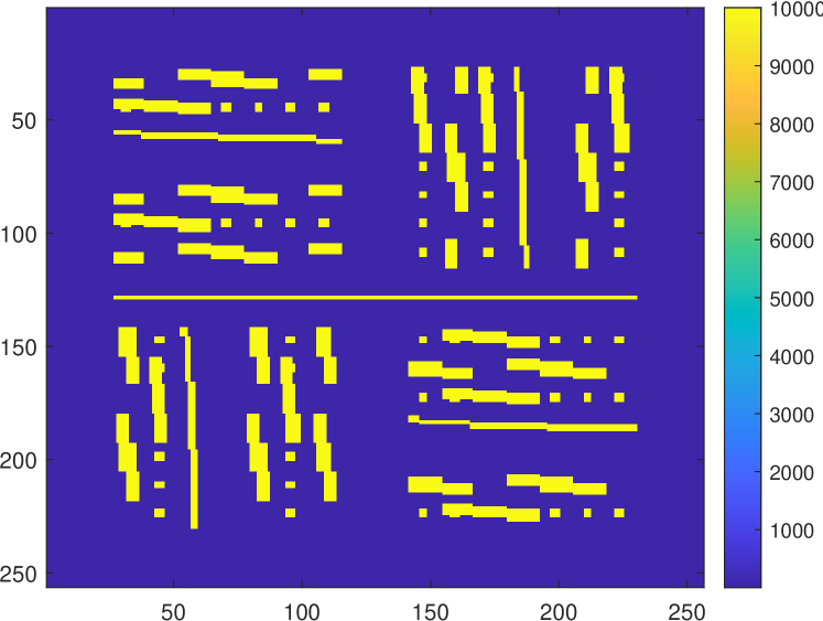
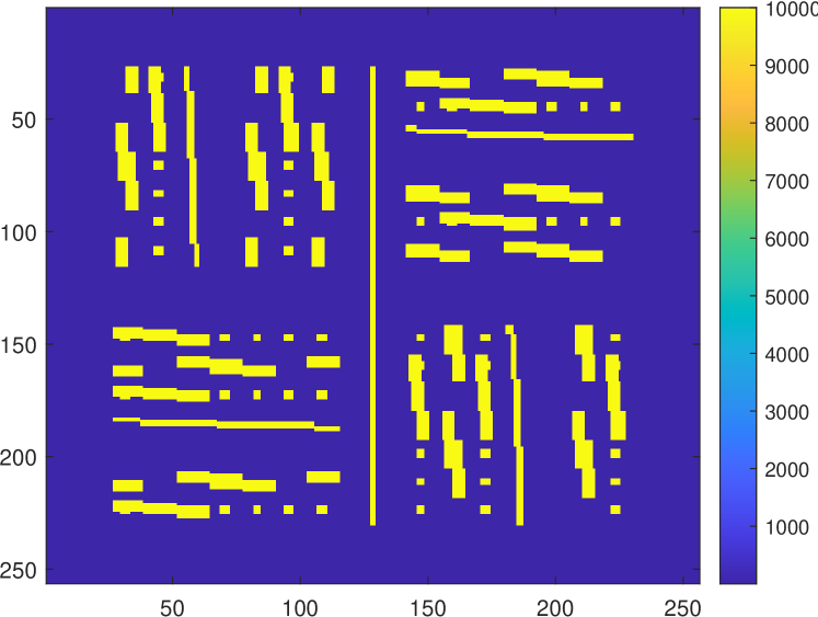
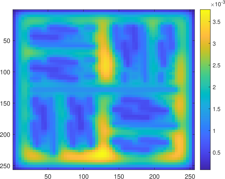
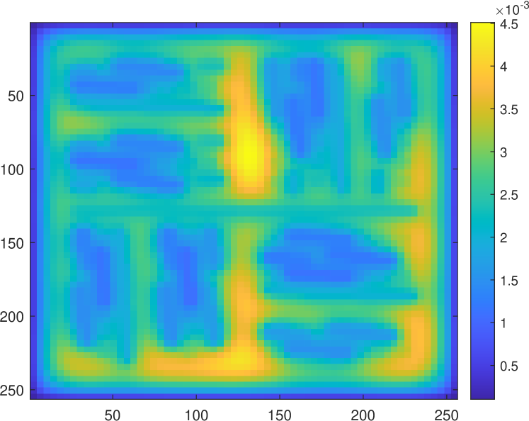
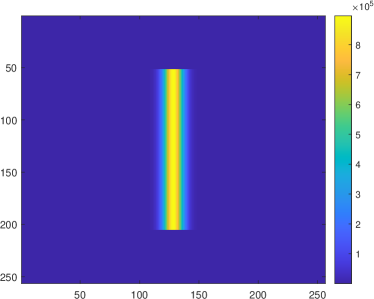
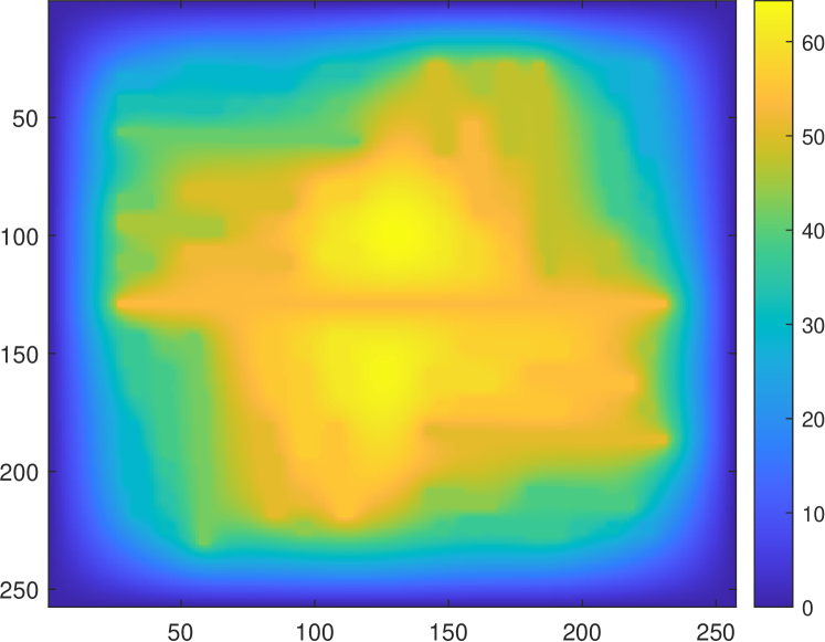
In all the experiments, we take the spatial domain to be Ω=(0,1)2Ωsuperscript012\Omega=(0,1)^{2} and the fine mesh size to be h=1/2561256h=1/256. An example of the media κ1subscript𝜅1\kappa_{1} and κ2subscript𝜅2\kappa_{2} used in the experiments is illustrated in Figure 3. In the figure, the contrast values, i.e. the ratio of the maximum and the minimum in ΩΩ\Omega, of the media are κ¯1=κ¯2=104subscript¯𝜅1subscript¯𝜅2superscript104\overline{\kappa}_{1}=\overline{\kappa}_{2}=10^{4}. Unless otherwise specified, we set σ=1𝜎1\sigma=1.

Refer to caption
(a) κ1subscript𝜅1\kappa_{1}
Refer to caption
(b) κ2subscript𝜅2\kappa_{2}
Figure 3: High contrast permeability field

5.1 Experiment 1 static case

In this experiment, we consider the dual continuum model under steady state

div(κ1p1)+σ(p1p2)=f1,div(κ2p2)σ(p1p2)=f2.formulae-sequencedivsubscript𝜅1subscript𝑝1𝜎subscript𝑝1subscript𝑝2subscript𝑓1divsubscript𝜅2subscript𝑝2𝜎subscript𝑝1subscript𝑝2subscript𝑓2\begin{split}-\text{div}(\kappa_{1}\nabla p_{1})+\sigma(p_{1}-p_{2})=f_{1},\\ -\text{div}(\kappa_{2}\nabla p_{2})-\sigma(p_{1}-p_{2})=f_{2}.\end{split} (102)

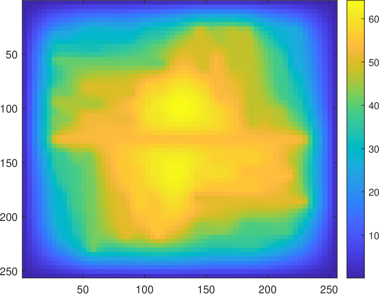
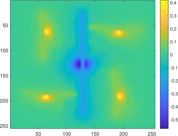
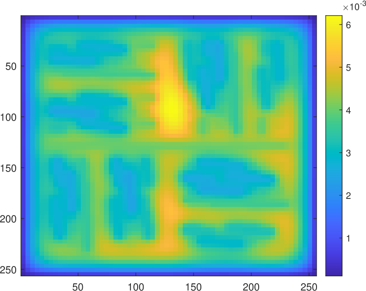
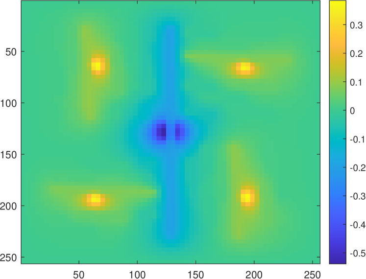
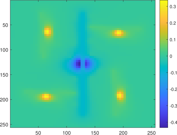
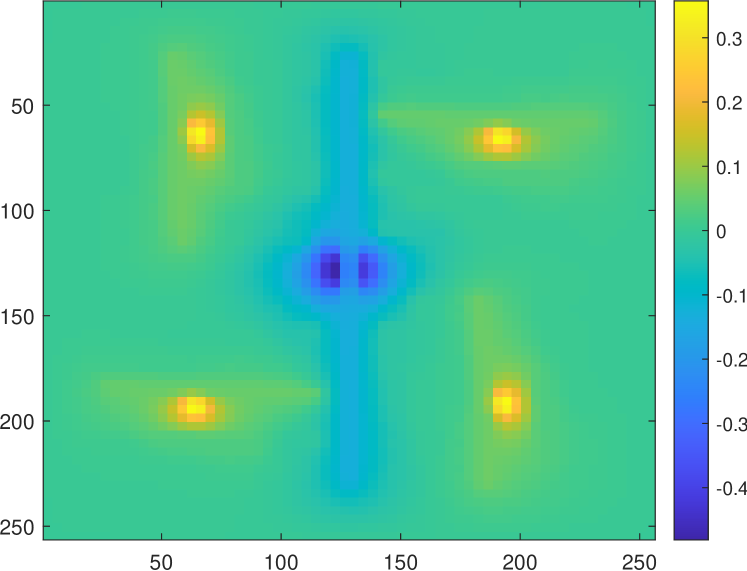
The source terms are given as f1(x,y)=1subscript𝑓1𝑥𝑦1f_{1}(x,y)=1 and f2(x,y)subscript𝑓2𝑥𝑦f_{2}(x,y) as shown in Figure 4. In Figure 5, we plot the fine-scale solution, the coarse-scale average and the NLMC coarse-scale solution with coarse mesh size H=1/64𝐻164H=1/64 and number of oversampling layers m=8𝑚8m=8, from which we observe very good agreement between the coarse-scale average and the NLMC solution. In Table 1, we present the relative L2superscript𝐿2L^{2} error with varying coarse grid size. With the number of oversampling layers satisfying the sufficient condition, we can see that the error converges. We also compare the performance of different numbers of oversampling layers under fixed coarse mesh size H𝐻H. The results are summarized in Table 2 for H=1/32𝐻132H=1/32 and Table 3 for H=1/64𝐻164H=1/64. It can be seen that the error decays quickly with respect to the number of oversampling layers m𝑚m for both cases, which verifies the fact that the oversampling region has to be sufficiently large to obtain quality numerical approximations.
Refer to caption
Figure 4: Source term f2subscript𝑓2f_{2} in Experiment 1.
Refer to caption
Refer to caption
Refer to caption
Refer to caption
Refer to caption
Refer to caption
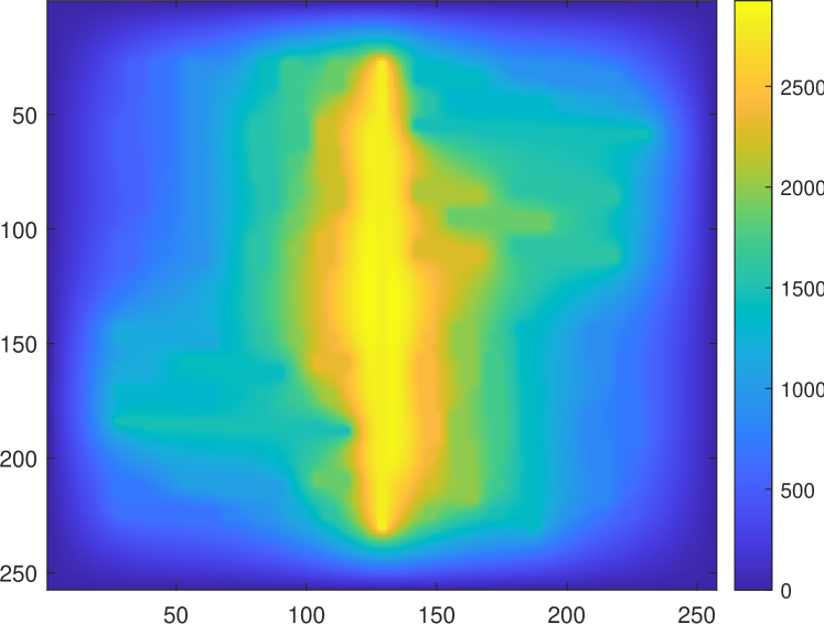
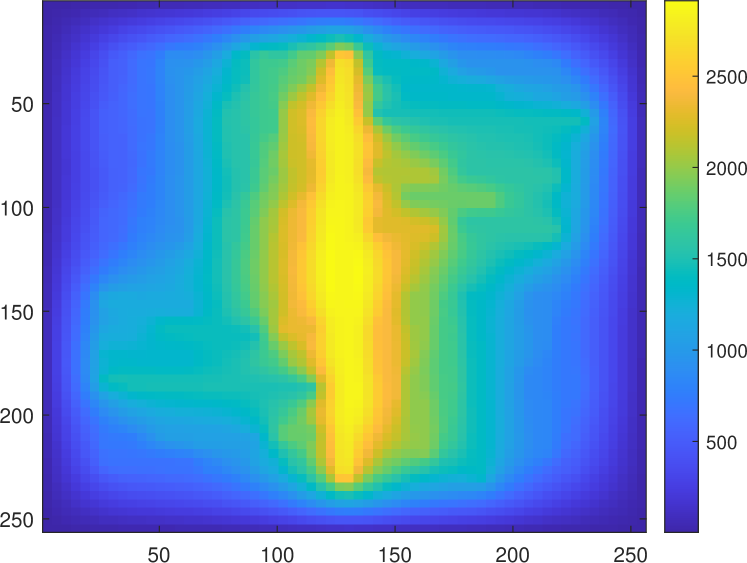
Figure 5: Plots of the numerical approximations of pressure with coarse mesh size H=1/64𝐻164H=1/64 and m=8𝑚8m=8 oversampling layers in Experiment 1. Left: first continuum. Right: second continuum. First row: fine-scale solution. Second row: coarse-scale average of fine-scale solution. Third row: NLMC solution.
H𝐻H m𝑚m eL2(1)superscriptsubscript𝑒superscript𝐿21e_{L^{2}}^{(1)} eL2(2)superscriptsubscript𝑒superscript𝐿22e_{L^{2}}^{(2)}
1/8 3 96.7318% 88.9818%
1/16 5 32.3229% 19.3473%
1/32 6 0.6045% 0.3680%
1/64 8 0.0550% 0.0296%
Table 1: Convergence of eL2subscript𝑒subscript𝐿2e_{L_{2}} with respect to coarse mesh size H𝐻H in Experiment 1.
m𝑚m Area Ratio eL2(1)superscriptsubscript𝑒superscript𝐿21e_{L^{2}}^{(1)} eL2(2)superscriptsubscript𝑒superscript𝐿22e_{L^{2}}^{(2)}
3 4.79% 99.3677% 93.9357%
4 7.91% 76.6083% 55.1631%
5 11.81% 8.6605% 5.3115%
6 16.50% 0.6045% 0.3680%
Table 2: Comparison of eL2subscript𝑒subscript𝐿2e_{L_{2}} error with different number of oversampling layers m𝑚m for H=1/32𝐻132H=1/32 in Experiment 1.
m𝑚m Area Ratio eL2(1)superscriptsubscript𝑒superscript𝐿21e_{L^{2}}^{(1)} eL2(2)superscriptsubscript𝑒superscript𝐿22e_{L^{2}}^{(2)}
2 0.61% 99.9102% 97.9631%
4 1.98% 99.1268% 91.9240%
6 4.13% 11.8898% 6.3181%
7 5.49% 0.7959% 0.4219%
8 7.06% 0.0550% 0.0296%
Table 3: Comparison of eL2subscript𝑒subscript𝐿2e_{L_{2}} error with different number of oversampling layers m𝑚m for H=1/64𝐻164H=1/64 in Experiment 1.

5.2 Experiment 2: time-dependent case

The time dependent case faces the similar issue with the error. f1(x,y)=1subscript𝑓1𝑥𝑦1f_{1}(x,y)=1 and f2(x,y)subscript𝑓2𝑥𝑦f_{2}(x,y) is depicted in Figure 6, which represents a simplified five-spot well rate. The temporal domain is [0,T]0𝑇[0,T] with final time T=5𝑇5T=5. In Figure 7, we plot the fine-scale solution, the coarse-scale average and the NLMC coarse-scale solution with coarse mesh size H=1/64𝐻164H=1/64 and number of oversampling layers m=8𝑚8m=8. Again, the NLMC solution is a good approximation for the coarse-scale average. In Figure 8, we depict the change of pressure at different time steps. In Table 4, we present the relative L2superscript𝐿2L^{2} error with varying coarse grid size. Again, with the number of oversampling layers satisfying the sufficient condition, we can see that the error converges very well.
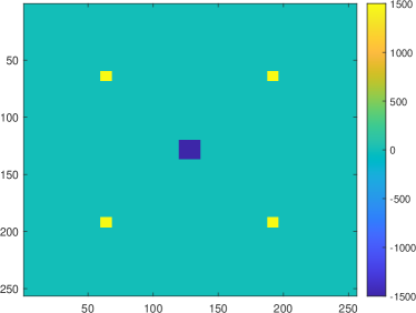
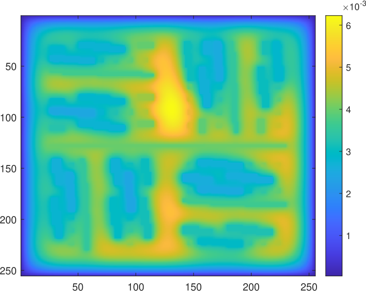
Refer to caption
Figure 6: Source term f2subscript𝑓2f_{2} in Experiment 2.
Refer to caption
Refer to caption
Refer to caption
Refer to caption
Refer to caption
Refer to caption
Figure 7: Plots of the numerical approximations of final-time pressure with coarse mesh size H=1/64𝐻164H=1/64 and m=8𝑚8m=8 oversampling layers in Experiment 2. Left: first continuum. Right: second continuum. First row: fine-scale solution. Second row: coarse-scale average of fine-scale solution. Third row: NLMC solution.
H𝐻H m𝑚m eL2(1)superscriptsubscript𝑒superscript𝐿21e_{L^{2}}^{(1)} eL2(2)superscriptsubscript𝑒superscript𝐿22e_{L^{2}}^{(2)}
1/8 3 20.6422% 58.4975%
1/16 5 1.1245% 2.6226%
1/32 6 0.0254% 0.0717%
1/64 8 0.0017% 0.0037%
Table 4: Convergence of eL2subscript𝑒subscript𝐿2e_{L_{2}} with respect to coarse mesh size H𝐻H in Experiment 2.
Refer to caption
Refer to caption
Refer to caption
Refer to caption
Refer to caption
Refer to caption
Figure 8: Plots of the NLMC numerical approximations of pressure at various time instants with coarse mesh size H=1/64𝐻164H=1/64 and m=8𝑚8m=8 oversampling layers in Experiment 2. Left: first continuum. Right: second continuum. First row: t=1.25𝑡1.25t=1.25. Second row: t=2.5𝑡2.5t=2.5. Third row: t=5𝑡5t=5.

6 Conclusions

In this paper, we investigated the non-local multicontinuum (NLMC) upscaling method for a dual continuum model in fractured porous media. Localized multiscale basis functions that separate each continuum are constructed. To find the basis, we solve local problems subject to energy minimization constraints in oversampling coarse regions. It is showed that the basis functions equip the method with coarse mesh convergence. Some numerical examples are presented to support the theory. The numerical examples also indicate that the proposed method provides accurate and efficient coarse-grid approximation.

References

  • [1] A. Abdulle. On a priori error analysis of fully discrete heterogeneous multiscale fem. SIAM J. Multiscale Modeling and Simulation, 4(2):447–459, 2005.
  • [2] Todd Arbogast, Jim Douglas, Jr, and Ulrich Hornung. Derivation of the double porosity model of single phase flow via homogenization theory. SIAM Journal on Mathematical Analysis, 21(4):823–836, 1990.
  • [3] GI Barenblatt, Iu P Zheltov, and IN Kochina. Basic concepts in the theory of seepage of homogeneous liquids in fissured rocks [strata]. Journal of applied mathematics and mechanics, 24(5):1286–1303, 1960.
  • [4] Victor Calo, Yalchin Efendiev, and Juan Galvis. A note on variational multiscale methods for high-contrast heterogeneous porous media flows with rough source terms. Advances in water resources, 34(9):1177–1185, 2011.
  • [5] Siu Wun Cheung, Eric T. Chung, Yalchin Efendiev, and Wing Tat Leung. Explicit and energy-conserving constraint energy minimizing generalized multiscale discontinuous galerkin method for wave propagation in heterogeneous media. arXiv preprint, arXiv:2009.00991, 2020.
  • [6] Siu Wun Cheung, Eric T Chung, Yalchin Efendiev, Wing Tat Leung, and Maria Vasilyeva. Constraint energy minimizing generalized multiscale finite element method for dual continuum model. Communications in Mathematical Sciences, 18:663–685, 2020.
  • [7] Siu Wun Cheung, Eric T Chung, and Wing Tat Leung. Constraint energy minimizing generalized multiscale discontinuous galerkin method. Journal of Computational & Applied Mathematics, 380:112960, 2020.
  • [8] Eric Chung, Yalchin Efendiev, and Thomas Y Hou. Adaptive multiscale model reduction with generalized multiscale finite element methods. Journal of Computational Physics, 320:69–95, 2016.
  • [9] Eric Chung, Yalchin Efendiev, and Wing Tat Leung. Constraint energy minimizing generalized multiscale finite element method in the mixed formulation. Computational Geosciences, 22(3):677–693, 2018.
  • [10] Eric T Chung, Yalchin Efendiev, Tat Leung, and Maria Vasilyeva. Coupling of multiscale and multi-continuum approaches. GEM-International Journal on Geomathematics, 8(1):9–41, 2017.
  • [11] Eric T Chung, Yalchin Efendiev, and Wing Tat Leung. Constraint energy minimizing generalized multiscale finite element method. Computer Methods in Applied Mechanics and Engineering, 339:298–319, 2018.
  • [12] Eric T. Chung, Yalchin Efendiev, Wing Tat Leung, Yating Wang, and Maria Vasilyeva. Non-local multi-continua upscaling for flows in heterogeneous fractured media. Journal of Computational Physics, 372:22–34, 2018.
  • [13] ET Chung, Y Efendiev, and G Li. An adaptive GMsFEM for high-contrast flow problems. Journal of Computational Physics, 273:54–76, 2014.
  • [14] Jim Douglas Jr and T Arbogast. Dual porosity models for flow in naturally fractured reservoirs. Dynamics of Fluids in Hierarchical Porous Media, pages 177–221, 1990.
  • [15] L.J. Durlofsky. Numerical calculation of equivalent grid block permeability tensors for heterogeneous porous media. Water Resour. Res., 27:699–708, 1991.
  • [16] W. E and B. Engquist. Heterogeneous multiscale methods. Comm. Math. Sci., 1(1):87–132, 2003.
  • [17] W. E, P. Ming, and P. Zhang. Analysis of the heterogeneous multiscale method for elliptic homogenization problems. J. Amer. Math. Soc., 18(1):121–156, 2005.
  • [18] Y. Efendiev, J. Galvis, and T. Hou. Generalized multiscale finite element methods. Journal of Computational Physics, 251:116–135, 2013.
  • [19] Y. Efendiev, J. Galvis, and X.H. Wu. Multiscale finite element methods for high-contrast problems using local spectral basis functions. Journal of Computational Physics, 230:937–955, 2011.
  • [20] Y. Efendiev, T. Hou, and X.H. Wu. Convergence of a nonconforming multiscale finite element method. SIAM J. Numer. Anal., 37:888–910, 2000.
  • [21] Yalchin Efendiev, Eduardo Gildin, and Yanfang Yang. Online adaptive local-global model reduction for flows in heterogeneous porous media. Computation, 4(2):22, 2016.
  • [22] TT Garipov, M Karimi-Fard, and HA Tchelepi. Discrete fracture model for coupled flow and geomechanics. Computational Geosciences, 20(1):149–160, 2016.
  • [23] T. Hou and X.H. Wu. A multiscale finite element method for elliptic problems in composite materials and porous media. J. Comput. Phys., 134:169–189, 1997.
  • [24] T.J.R. Hughes, G.R. Feijóo, L. Mazzei, and J.-B. Quincy. The variational multiscale method - a paradigm for computational mechanics. Comput. Methods Appl. Mech Engrg., 127:3–24, 1998.
  • [25] TJR Hughes and G Sangalli. Variational multiscale analysis: the fine-scale Green’s function, projection, optimization, localization, and stabilized methods. SIAM Journal on Numerical Analysis, 45(2):539–557, 2007.
  • [26] O. Iliev, R. Lazarov, and J. Willems. Variational multiscale finite element method for flows in highly porous media. Multiscale Model. Simul., 9(4):1350–1372, 2011.
  • [27] M Karimi-Fard, LJ Durlofsky, and K Aziz. An efficient discrete-fracture model applicable for general-purpose reservoir simulators. SPE-88812-PA, 2004.
  • [28] M Karimi-Fard and A Firoozabadi. Numerical simulation of water injection in 2d fractured media using discrete-fracture model. SPE-71615-MS, 2001.
  • [29] H Kazemi, LS Merrill Jr, KL Porterfield, PR Zeman, et al. Numerical simulation of water-oil flow in naturally fractured reservoirs. Society of Petroleum Engineers Journal, 16(06):317–326, 1976.
  • [30] Jun Sur Richard Park, Siu Wun Cheung, and Tina Mai. Multiscale simulations for multi-continuum richards equations. arXiv preprint, arXiv:2010.09181, 2020.
  • [31] Jun Sur Richard Park, Siu Wun Cheung, Tina Mai, and Viet Ha Hoang. Multiscale simulations for upscaled multi-continuum flows. Journal of Computational & Applied Mathematics, 374:112782, 2020.
  • [32] K Pruess and TN Narasimhan. On fluid reserves and the production of superheated steam from fractured, vapor-dominated geothermal reservoirs. Journal of Geophysical Research: Solid Earth, 87(B11):9329–9339, 1982.
  • [33] Maria Vasilyeva, Eric T Chung, Siu Wun Cheung, Yating Wang, and Georgy Prokopev. Nonlocal multicontinua upscaling for multicontinua flow problems in fractured porous media. Journal of Computational & Applied Mathematics, 355:258–267, 2019.
  • [34] Maria Vasilyeva, Eric T. Chung, Wing Tat Leung, and Valentin Alekseev. Nonlocal multicontinuum (nlmc) upscaling of mixed dimensional coupled flow problem for embedded and discrete fracture models. GEM International Journal on Geomathematics, 10:23, 2019.
  • [35] Min Wang, Siu Wun Cheung, Eric T. Chung, Maria Vasilyeva, and Yuhe Wang. Generalized multiscale multicontinuum model for fractured vuggy carbonate reservoirs. Journal of Computational and Applied Mathematics, 366:112370, 2020.
  • [36] JE Warren, P Jj Root, et al. The behavior of naturally fractured reservoirs. Society of Petroleum Engineers Journal, 3(03):245–255, 1963.
  • [37] X.H. Wu, Y. Efendiev, and T.Y. Hou. Analysis of upscaling absolute permeability. Discrete and Continuous Dynamical Systems, Series B., 2:158–204, 2002.
  • [38] Yu-Shu Wu, Karsten Pruess, et al. A multiple-porosity method for simulation of naturally fractured petroleum reservoirs. SPE Reservoir Engineering, 3(01):327–336, 1988.
  • [39] Lina Zhao and Eric Chung. An analysis of the nlmc upscaling method for high contrast problems. Journal of Computational and Applied Mathematics, 367:112480, 2020.