Nonuniversal interstellar density spectra probed by pulsars

Abstract

The Galactic interstellar turbulence affects the density distribution and star formation. We introduce a new method of measuring interstellar turbulent density spectra by using the dispersion measures (DMs) of a large sample of pulsars. Without the need of invoking multiple tracers, we obtain nonuniversal density spectra in the multi-phase interstellar medium over different ranges of length scales. By comparing the analytical structure function of DMs with the observationally measured one in different areas of sky, we find a shallow density spectrum arising from the supersonic turbulence in cold interstellar phases, and a Kolmogorov-like density spectrum in the diffuse warm ionized medium (WIM). Both spectra extend up to hundreds of pc. On larger scales, we for the first time identify a steep density spectrum in the diffuse WIM extending up to several kpc. Our results show that the DMs of pulsars can provide unique new information on the interstellar turbulence.

1. Introduction

Turbulence is ubiquitous in astrophysical media and occurs over a vast range of length scales. Observations show that the turbulent spectrum of electron density in the Galactic interstellar medium (ISM) extends from $10^{6}$ to $10^{18}$ m (Armstrong et al., 1995; Chepurnov & Lazarian, 2010; Lee & Lee, 2019). In the intergalactic medium, a turbulent spectrum of electron density up to $100$ Mpc has recently been inferred from the observations of fast radio bursts (Xu & Zhang, 2020). Turbulence participates and plays an essential role in a variety of fundamental astrophysical processes (Brandenburg & Lazarian, 2013).

The turbulence in the Galactic ISM and its astrophysical implications have been extensively studied (Elmegreen & Scalo, 2004; Scalo & Elmegreen, 2004). As one of its effects, turbulence shapes the density distribution in different interstellar phases and significantly influences star formation (Mac Low & Klessen, 2004; McKee & Ostriker, 2007). This is demonstrated by numerous studies on density statistics (e.g., Lithwick & Goldreich 2001; Padoan & Nordlund 2002; Beresnyak et al. 2005; Kowal et al. 2007; Burkhart et al. 2009; Federrath & Banerjee 2015; Kritsuk et al. 2017; Xu et al. 2019), which are more easily accessible to observations compared with the statistics of, e.g., velocity and magnetic field. The power spectra of density fluctuations is frequently used as a diagnostic of turbulence properties. For instance, the spectral slope is dependent on the sonic Mach number of turbulence (Kowal et al., 2007). The sonic Mach number varies in different interstellar phases (Zuckerman & Palmer, 1974; Heiles & Troland, 2003; Gaensler et al., 2011) and is believed to be an important parameter affecting the star formation rate (Federrath & Klessen, 2012). The small inner scale of a shallow density spectrum, where turbulent energy is dissipated, corresponds to the correlation length of density structures, while the large outer scale of a steep density spectrum, where turbulent energy is injected, indicates the driving scale of turbulence (Lazarian & Pogosyan, 2004, 2006).

The density spectra in different interstellar phases can be directly measured by using spatially continuous emission with the corresponding gas tracers and dust (Lazarian, 2009; Chepurnov & Lazarian, 2010; Hennebelle & Falgarone, 2012; Pingel et al., 2018). From the perspective of pulsar observations, a density spectrum over a wide range of length scales has been suggested based on interstellar scintillation and scattering for several decades (Lee & Jokipii, 1976; Armstrong et al., 1981, 1995). In particular, a shallow density spectrum in cold interstellar phases was identified from temporal broadening measurements of pulsars by Xu & Zhang (2017).

Different from earlier approaches to obtain interstellar density spectra, here we employ the dispersion measures (DMs) of pulsars and extract the underlying interstellar density spectra from the structure functions (SFs) of their DMs. The relation between the SF of projected quantities and the 3D power-law spectrum of their fluctuations was established by Lazarian & Pogosyan (2016) (hereafter LP16), which depends on the shallowness of the turbulent power-law spectrum and the thickness of the observed turbulent volume. The LP16 analytical approach was proposed for studying the Faraday rotation and synchrotron statistics of a spatially continuous synchrotron-emitting medium. It has been extended to point sources, including molecular cloud cores, fast radio bursts, radio sources, and a variety of observables, e.g., DMs, emission measures, velocities (Xu & Zhang, 2016; Xu, 2020; Xu & Zhang, 2020). In this work, we apply the LP16 approach to the DMs of pulsars. By using many lines of sight through the ISM toward a large number of pulsars, we are able to sample the turbulence in both warm and cold interstellar phases over a broad range of length scales, with no need to invoke multiple tracers. In Section 2, we present the formalism of the DM SF in different scenarios. In Section 3, we analyze the observations of pulsars with our statistical approach to obtain the interstellar density spectra. The discussion and conclusions are given in Section 4.

2. SF of DMs

We describe the statistically homogeneous electron density $n_{e}$ as a sum of the mean density $n_{e0}$ and a density fluctuation $\delta n_{e}$,

$$n_{e}=n_{e0}+\delta n_{e},$$ (1)

where $\delta n_{e}$ is a zero mean fluctuation. For electron density fluctuations induced by turbulence, the two-point correlation function (CF) takes the form (LP16),

$$\xi(R,\Delta l) =\langle\delta n_{e}(\bm{X_{1}},l_{1})\delta n_{e}(\bm{X_{2},},l_{2})\rangle$$ (2)

$$=\langle\delta n_{e}^{2}\rangle\frac{L_{i}^{m}}{L_{i}^{m}+(R^{2}+\Delta l^{2})^{\frac{m}{2}}},$$

where $\bm{X}$ is the position on the sky plane, $l$ is the distance along the line of sight (LOS), $R=|\bm{X_{1}}-\bm{X_{2}}|$, $\Delta l=l_{1}-l_{2}$, and $\langle...\rangle$ means an ensemble average. The statistical properties of $\delta n_{e}$ are described by the correlation length $L_{i}$ and the power-law index $m$. The latter is related to the spectral index of turbulence $\alpha$ by (Lazarian & Pogosyan, 2006),

$$\alpha= m-N,~{}~{}~{}~{}~{}~{}\alpha_{3D}>-3,~{}~{}\text{shallow},$$ (3a)

$$\alpha= -m-N,~{}~{}~{}\alpha_{3D}<-3,~{}~{}\text{steep},$$ (3b)

where $N$ is the dimensionality of space. A “shallow” spectrum with the 3D spectral index $\alpha_{3D}>-3$ is dominated by small-scale density fluctuations, while a “steep” spectrum with $\alpha_{3D}<-3$ is dominated by large-scale density fluctuation. In supersonic turbulence with local density enhancements due to shock compression, the density spectrum tends to be shallow (Beresnyak et al., 2005; Kowal et al., 2007). In subsonic turbulence, the steep Kolmogorov density spectrum with $\alpha_{3D}=-11/3$ is usually expected (Armstrong et al., 1995; Chepurnov & Lazarian, 2010).

As a handy observable of pulsars, the dispersion measure DM$=\int n_{e}dl$ is the column density of free electrons between the observer and the source. The SF of the DMs of a sample of point sources in a turbulent medium is

$$D(R,l_{1},l_{2}) =\langle[\text{DM}(\bm{X_{1}},l_{1})-\text{DM}(\bm{X_{2}},l_{2})]^{2}\rangle$$

$$=\Big{\langle}\Big{[}\int_{0}^{l_{1}}dln_{e}(\bm{X_{1}},l)-\int_{0}^{l_{2}}dln_{e}(\bm{X_{2}},l)\Big{]}^{2}\Big{\rangle}$$

$$=\Big{\langle}\Big{[}\int_{0}^{l_{1}}dl\delta n_{e}(\bm{X_{1}},l)-\int_{0}^{l_{2}}dl\delta n_{e}(\bm{X_{2}},l)\Big{]}^{2}\Big{\rangle}$$

$$~{}~{}~{}~{}~{}~{}+n_{e0}^{2}(\Delta l)^{2}$$

$$=D_{\delta n_{e}}(R,l_{1},l_{2})+n_{e0}^{2}(\Delta l)^{2}.$$ (4)

Here

$$D_{\delta n_{e}}(R,l_{1},l_{2})$$ (5)

$$= \Big{\langle}\Big{[}\int_{0}^{l_{1}}dl\delta n_{e}(\bm{X_{1}},l)-\int_{0}^{l_{2}}dl\delta n_{e}(\bm{X_{2}},l)\Big{]}^{2}\Big{\rangle}$$

is the SF of DM fluctuations, which contains the information about the statistical properties of turbulence. The second term in Eq. (4) comes from the difference between the distances of a pair of point sources, and its value depends on $n_{e0}$.

The approximate expression of $D_{\delta n_{e}}(R,l_{1},l_{2})$ is (LP16)

$$D_{\delta n_{e}}(R,l_{1},l_{2})\approx 2D^{+}(R,l_{+})+\frac{1}{2}\Lambda(\Delta l)^{2},$$ (6)

with

$$D^{+}(R,l_{+}) =2\langle\delta n_{e}^{2}\rangle\int_{0}^{l_{+}}d\Delta l(l_{+}-\Delta l)$$ (7)

$$~{}~{}~{}~{}~{}~{}\Bigg{[}\frac{L_{i}^{m}}{L_{i}^{m}+\Delta l^{m}}-\frac{L_{i}^{m}}{L_{i}^{m}+(R^{2}+\Delta l^{2})^{\frac{m}{2}}}\Bigg{]},$$

and

$$\Lambda =\xi(0,l_{+})-\xi(R,l_{+})+2\xi(R,0)$$

$$=\langle\delta n_{e}^{2}\rangle\Bigg{[}\frac{L_{i}^{m}}{L_{i}^{m}+l_{+}^{m}}-\frac{L_{i}^{m}}{L_{i}^{m}+(R^{2}+l_{+}^{2})^{\frac{m}{2}}}$$

$$~{}~{}~{}~{}+2\frac{L_{i}^{m}}{L_{i}^{m}+R^{m}}\Bigg{]},$$ (8)

where $l_{+}=(l_{1}+l_{2})/2$. We next consider the simplified expressions of $D_{\delta n_{e}}(R,l_{1},l_{2})$ in different cases.

2.1. Case 1: $l_{+}>L_{i}$ and a shallow density spectrum

When $l_{+}>L_{i}$, $D^{+}(R,l_{+})$ in Eq. (7) has asymptotic expressions in different regimes (LP16),

$$D^{+}(R,l_{+})\approx 2\langle\delta n_{e}^{2}\rangle L_{i}^{-m}l_{+}R^{m+1},~{}~{}~{}~{}~{}~{}R<L_{i},$$ (9a)

$$D^{+}(R,l_{+})\approx 2\langle\delta n_{e}^{2}\rangle L_{i}^{m}l_{+}R^{-m+1},L_{i}<R<l_{+},$$ (9b)

$$D^{+}(R,l_{+})\approx 2\langle\delta n_{e}^{2}\rangle L_{i}^{m}l_{+}^{-m+2},~{}~{}~{}~{}~{}~{}~{}~{}~{}~{}~{}R>l_{+}.$$ (9c)

Here only Eqs. (9b) and (9c) apply to the case of a shallow density spectrum, which has the inner scale as $L_{i}$. Approximately, $\Lambda$ in Eq. (2) at $l_{+}>L_{i}$ becomes

$$\Lambda\approx 2\langle\delta n_{e}^{2}\rangle,~{}~{}~{}~{}~{}~{}R<L_{i},$$ (10a)

$$\Lambda\approx 0,~{}~{}~{}~{}~{}~{}~{}~{}~{}~{}~{}~{}~{}~{}~{}~{}R>L_{i},$$ (10b)

where we adopt Eq. (10b) for the inertial range of turbulence. Therefore, we have $D(R,l_{1},l_{2})$ as

$$D(R,l_{1},l_{2})\approx 4\langle\delta n_{e}^{2}\rangle L_{i}^{m}l_{+}R^{-m+1}+n_{e0}^{2}(\Delta l)^{2},$$

$$D(R,l_{1},l_{2})\approx ~{}~{}~{}~{}~{}~{}~{}~{}~{}~{}~{}~{}~{}~{}~{}~{}~{}~{}~{}~{}~{}~{}~{}~{}~{}~{}~{}~{}~{}L_{i}<R<l_{+},$$ (11a)

$$D(R,l_{1},l_{2})\approx 4\langle\delta n_{e}^{2}\rangle L_{i}^{m}l_{+}^{-m+2}+n_{e0}^{2}(\Delta l)^{2},$$

$$D(R,l_{1},l_{2})\approx ~{}~{}~{}~{}~{}~{}~{}~{}~{}~{}~{}~{}~{}~{}~{}~{}~{}~{}~{}~{}~{}~{}~{}~{}~{}~{}~{}~{}~{}~{}~{}~{}~{}~{}~{}~{}~{}R>l_{+}.$$ (11b)

When we consider a sample of point sources with different distances, $l_{+}$ and $\Delta l$ are in the ranges $[L_{i}+|\Delta l|/2,L-|\Delta l|/2]$ and $[L_{i}-L,L-L_{i}]$, respectively. Here $L$ is the thickness of the turbulent volume sampled by the point sources. We replace $l_{+}$ and $(\Delta l)^{2}$ with their averages $\langle l_{+}\rangle=(L+L_{i})/2$ and $\langle(\Delta l)^{2}\rangle=1/3(L-L_{i})^{2}$ in Eq. (11b) and obtain

$$D(R)\approx 2\langle\delta n_{e}^{2}\rangle L_{i}^{m}(L+L_{i})R^{-m+1}+\frac{1}{3}n_{e0}^{2}(L-L_{i})^{2},$$

$$D(R)\approx ~{}~{}~{}~{}~{}~{}~{}~{}~{}~{}~{}~{}~{}~{}~{}~{}~{}~{}~{}~{}~{}~{}~{}~{}~{}~{}~{}~{}~{}~{}~{}~{}~{}~{}~{}~{}~{}L_{i}\lesssim R\lesssim\frac{L+L_{i}}{2},$$ (12a)

$$D(R)\approx 4\langle\delta n_{e}^{2}\rangle L_{i}^{m}\bigg{(}\frac{L+L_{i}}{2}\bigg{)}^{-m+2}+\frac{1}{3}n_{e0}^{2}(L-L_{i})^{2},$$

$$D(R)\approx ~{}~{}~{}~{}~{}~{}~{}~{}~{}~{}~{}~{}~{}~{}~{}~{}~{}~{}~{}~{}~{}~{}~{}~{}~{}~{}~{}~{}~{}~{}~{}~{}~{}~{}~{}~{}~{}~{}~{}~{}~{}~{}~{}~{}~{}~{}R\gtrsim\frac{L+L_{i}}{2}.$$ (12b)

Only when the first term dominates over the second term in Eq. (12a), can the scaling of turbulence be seen. The scale where $D(R)$ saturates depends on $L$. We stress the approximate nature of Eq. (12b), as it results from the average over a sample of point sources with different distances.

2.2. Case 2: $l_{+}>L_{i}$ and a steep density spectrum

A steep density spectrum has the outer scale as $L_{i}$. Hence, only Eq. (9a) is applicable for $D^{+}(R,l_{+})$. $D^{+}(R,l_{+})$ tends to saturate at $R=L_{i}$ and remain constant at a larger $R$. Likewise, we should only use Eq. (10a) for $\Lambda$. Then $D(R,l_{1},l_{2})$ has the form,

$$D(R,l_{1},l_{2})\approx 4\langle\delta n_{e}^{2}\rangle L_{i}^{-m}l_{+}R^{m+1}$$

$$D(R,l_{1},l_{2})\approx +\big{(}\langle\delta n_{e}^{2}\rangle+n_{e0}^{2}\big{)}(\Delta l)^{2},~{}~{}~{}R<L_{i},$$ (13a)

$$D(R,l_{1},l_{2})\approx 4\langle\delta n_{e}^{2}\rangle L_{i}l_{+}+\big{(}\langle\delta n_{e}^{2}\rangle+n_{e0}^{2}\big{)}(\Delta l)^{2},$$

$$D(R,l_{1},l_{2})\approx ~{}~{}~{}~{}~{}~{}~{}~{}~{}~{}~{}~{}~{}~{}~{}~{}~{}~{}~{}~{}~{}~{}~{}~{}~{}~{}~{}~{}~{}~{}~{}~{}~{}~{}~{}~{}~{}~{}~{}~{}~{}R>L_{i}.$$ (13b)

Similar to Case 1, we take the averages of $l_{+}$ and $(\Delta l)^{2}$ and find,

$$D(R)\approx 2\langle\delta n_{e}^{2}\rangle L_{i}^{-m}(L+L_{i})R^{m+1}$$

$$D(R)\approx +\frac{1}{3}\big{(}\langle\delta n_{e}^{2}\rangle+n_{e0}^{2}\big{)}(L-L_{i})^{2},~{}~{}~{}~{}~{}~{}~{}~{}~{}R\lesssim L_{i},$$ (14a)

$$D(R)\approx 2\langle\delta n_{e}^{2}\rangle L_{i}(L+L_{i})+\frac{1}{3}\big{(}\langle\delta n_{e}^{2}\rangle+n_{e0}^{2}\big{)}(L-L_{i})^{2},$$

$$D(R)\approx ~{}~{}~{}~{}~{}~{}~{}~{}~{}~{}~{}~{}~{}~{}~{}~{}~{}~{}~{}~{}~{}~{}~{}~{}~{}~{}~{}~{}~{}~{}~{}~{}~{}~{}~{}~{}~{}~{}~{}~{}~{}~{}~{}~{}~{}~{}~{}~{}~{}~{}~{}~{}~{}~{}~{}~{}~{}R\gtrsim L_{i}.$$ (14b)

We note that $D(R)$ in Eq. (14a) has a steeper scaling with $R$ than that in Eq. (12a). The scales where $D(R)$ saturates in the two cases are also different.

2.3. Case 3: $l_{+}<L_{i}$ and a steep density spectrum

When the distances of the sources are smaller than $L_{i}$, $D^{+}(R,l_{+})$ has asymptotic expressions (LP16),

$$D^{+}(R,l_{+})\approx 2\langle\delta n_{e}^{2}\rangle L_{i}^{-m}l_{+}R^{m+1},~{}~{}~{}~{}~{}R<l_{+},$$ (15a)

$$D^{+}(R,l_{+})\approx 2\langle\delta n_{e}^{2}\rangle L_{i}^{-m}l_{+}^{2}R^{m},~{}~{}l_{+}<R<L_{i},$$ (15b)

$$D^{+}(R,l_{+})\approx 2\langle\delta n_{e}^{2}\rangle l_{+}^{2},~{}~{}~{}~{}~{}~{}~{}~{}~{}~{}~{}~{}~{}~{}~{}~{}~{}~{}~{}~{}~{}~{}~{}~{}~{}R>L_{i}.$$ (15c)

$\Lambda$ can also be approximately simplified as,

$$\Lambda\approx 2\langle\delta n_{e}^{2}\rangle,~{}~{}~{}~{}~{}~{}R<L_{i},$$ (16a)

$$\Lambda\approx \langle\delta n_{e}^{2}\rangle,~{}~{}~{}~{}~{}~{}~{}~{}R>L_{i}.$$ (16b)

The case with $l_{+}<L_{i}$ is only applicable for a steep density spectrum. Accordingly, in the above expression we can only use Eq. (16a), So there is

$$D(R,l_{1},l_{2})\approx 4\langle\delta n_{e}^{2}\rangle L_{i}^{-m}l_{+}R^{m+1}$$

$$D(R,l_{1},l_{2})\approx +\big{(}\langle\delta n_{e}^{2}\rangle+n_{e0}^{2}\big{)}(\Delta l)^{2},~{}~{}~{}~{}~{}~{}~{}~{}R<l_{+},$$ (17a)

$$D(R,l_{1},l_{2})\approx 4\langle\delta n_{e}^{2}\rangle L_{i}^{-m}l_{+}^{2}R^{m}+\big{(}\langle\delta n_{e}^{2}\rangle+n_{e0}^{2}\big{)}(\Delta l)^{2},$$

$$D(R,l_{1},l_{2})\approx ~{}~{}~{}~{}~{}~{}~{}~{}~{}~{}~{}~{}~{}~{}~{}~{}~{}~{}~{}~{}~{}~{}~{}~{}~{}~{}~{}~{}~{}~{}~{}~{}~{}~{}~{}~{}l_{+}<R<L_{i},$$ (17b)

$$D(R,l_{1},l_{2})\approx 4\langle\delta n_{e}^{2}\rangle l_{+}^{2}+\big{(}\langle\delta n_{e}^{2}\rangle+n_{e0}^{2}\big{)}(\Delta l)^{2},$$

$$D(R,l_{1},l_{2})\approx ~{}~{}~{}~{}~{}~{}~{}~{}~{}~{}~{}~{}~{}~{}~{}~{}~{}~{}~{}~{}~{}~{}~{}~{}~{}~{}~{}~{}~{}~{}~{}~{}~{}~{}~{}~{}~{}~{}~{}~{}~{}~{}~{}~{}~{}~{}R>L_{i}.$$ (17c)

The steepening of the $D(R,l_{1},l_{2})$-$R$ relation at $R<l_{+}$ comes from the projection effect when the turbulent volume in the LOS direction is relatively thick (see also Case 2). This feature can be used to determine the LOS thickness of a turbulence layer in observations (Lazarian & Pogosyan, 2000; Elmegreen et al., 2001; Padoan et al., 2001).

Based on the above result, we take the average of $l_{+}$ over the range $[|\Delta l|/2,L-|\Delta l|/2]$ and the average of $(\Delta l)^{2}$ over the range $[-L,L]$, i.e., $\langle l_{+}\rangle=L/2$ and $\langle(\Delta l)^{2}\rangle=1/3L^{2}$, where $L<L_{i}$, and find

$$D(R)\approx 2\langle\delta n_{e}^{2}\rangle L_{i}^{-m}LR^{m+1}+\frac{1}{3}\big{(}\langle\delta n_{e}^{2}\rangle+n_{e0}^{2}\big{)}L^{2},$$

$$D(R)\approx ~{}~{}~{}~{}~{}~{}~{}~{}~{}~{}~{}~{}~{}~{}~{}~{}~{}~{}~{}~{}~{}~{}~{}~{}~{}~{}~{}~{}~{}~{}~{}~{}~{}~{}~{}~{}~{}~{}~{}~{}~{}~{}~{}~{}~{}~{}~{}~{}~{}~{}~{}R\lesssim\frac{L}{2},$$ (18a)

$$D(R)\approx \langle\delta n_{e}^{2}\rangle L_{i}^{-m}L^{2}R^{m}+\frac{1}{3}\big{(}\langle\delta n_{e}^{2}\rangle+n_{e0}^{2}\big{)}L^{2},$$

$$D(R)\approx ~{}~{}~{}~{}~{}~{}~{}~{}~{}~{}~{}~{}~{}~{}~{}~{}~{}~{}~{}~{}~{}~{}~{}~{}~{}~{}~{}~{}~{}~{}~{}~{}~{}~{}~{}~{}~{}~{}~{}~{}~{}~{}\frac{L}{2}\lesssim R\lesssim L_{i},$$ (18b)

$$D(R)\approx \langle\delta n_{e}^{2}\rangle L^{2}+\frac{1}{3}\big{(}\langle\delta n_{e}^{2}\rangle+n_{e0}^{2}\big{)}L^{2},~{}R\gtrsim L_{i}.$$ (18c)

The above approximate expressions of $D(R)$ in different cases can be applied to a realistic situation with unknown distances of many point sources. Depending on the slope of the observationally measured SF and the LOS thickness of the turbulent medium relative to the transverse separation $R$ between lines of sight, the formula of $D(R)$ in the corresponding regime should be used.

3. Interstellar density spectra

The Wisconsin H-Alpha Mapper (WHAM) data (Haffner et al., 2003, 2010) reveal the complex structure of the interstellar ionized hydrogen content (see Fig 1). The discrete bright clumps indicate H II regions and are associated with massive star formation in the Galactic disk. The diffuse H$\alpha$ emission arises from the warm ionized medium (WIM). The electron density fluctuations in the WIM obtained from the WHAM data were found to have a Kolmogorov power spectrum (Chepurnov & Lazarian, 2010), as a remarkable extension of the Big Power Law in the sky earlier derived from interstellar scintillations and scattering in the local ISM ($\lesssim 1$ kpc) (Armstrong et al., 1995).

The DMs of Galatic pulsars are the integrals of $n_{e}$ along many different paths through the ISM. Their SF can be used to study the fluctuations in DMs on different length scales in the multi-phase ISM, from which we can extract the statistical properties of $\delta n_{e}$ induced by the interstellar turbulence. For the SF analysis, we take 2719 pulsars from the ATNF Pulsar Catalogue with DM measurements (Manchester et al., 2005). From Fig. 1, we see that they are primarily distributed in the Galactic disk toward the inner Galaxy. Different from the statistical analysis by using H$\alpha$ emission, as the lines of sight to pulsars pass through both warm and cold phases of the ISM, the DM SF of pulsars can probe various turbulence characteristics in different interstellar phases.

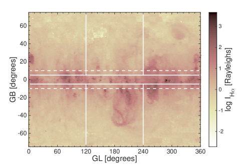
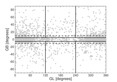
Figure 1.— (a) H$\alpha$ emission from WHAM sky survey. The color scale represents the logarithmic velocity-integrated intensity. (b) All sky map of pulsars from the ATNF Pulsar Catalogue. “GL” and “GB” represent Galactic longitude and Galactic latitude.

We first measure the DM SF of all pulsars over the whole sky,

$$D_{\text{DM}}(\theta)=\langle[\text{DM}(\bm{X_{1}})-\text{DM}(\bm{X_{2}})]^{2}\rangle,$$ (19)

where $\bm{X}$ is the position of a pulsar in the sky, $\theta$ is the angular separation between pulsars, and the average is computed over all pulsar pairs with the same $\theta$. The angular separations are binned evenly on a logarithmic scale within the range $2.5^{\circ}<\theta<150.8^{\circ}$. In Fig. 2, we see a basically flat DM SF with an insignificant dependence on $\theta$. It is mainly contributed by the DMs of the pulsars at $|\text{GB}|<5^{\circ}$ toward the inner Galaxy (see Fig. 2). Near the midplane of the Galactic disk, the measured $\delta n_{e}$ is too much contaminated by H II regions and spiral arms (Ocker et al., 2020), and the assumption of statistically homogeneous $n_{e}$ used in Eq. (1) is not appropriate. Since the information of interstellar turbulence cannot be effectively extracted from the DMs of very low-latitude pulsars, we next examine the DM SF of the pulsars at higher latitudes.

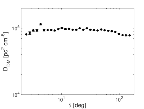
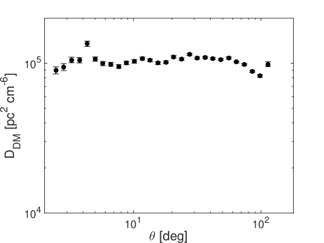
Figure 2.— (a) DM SF for all pulsars. (b) DM SF for the pulsars in the inner Galactic disk with $|\text{GB}|<5^{\circ}$, GL$<60^{\circ}$, and GL$>300^{\circ}$.

(1) The interstellar turbulence in cold phases with a shallow density spectrum ($|\text{GB}|>5^{\circ}$).

In Fig. 3, we present the DM SF for the pulsars at GB$>5^{\circ}$ (as indicated as the horizontal solid lines in Fig. 1). The error bars indicate $95\%$ confidence intervals. Here and elsewhere in this paper, all uncertainties are given at $95\%$ confidence. The fit to the data gives

$$D_{\text{DM}}(2.5^{\circ}<\theta<23.8^{\circ})[\text{pc}^{2}\text{cm}^{-6}]$$ (20)

$$= 2.2\times 10^{3}\pm 3.6\times 10^{2}(\theta[^{\circ}])^{0.25\pm 0.07}.$$

We take the value of $\theta$ where $D_{\text{DM}}$ seems to saturate as the upper bound of the fitting range. The fitted power law corresponds to a shallow density spectrum in Case 1 in Section 2. To compare with the analytical expression in Eq. (12b), we adopt $\theta=R/L$ under the assumption of statistically homogeneous density distribution. We determine the value of $L$ by using the peak of the pulsar distance distribution, i.e., $L\approx 2.0$ kpc (see Fig. 3). The pulsar distance Dist is also provided by the ATNF Pulsar Catalogue, whose default value is derived based on the YMW16 Galactic electron density model (Yao et al., 2017). Here and below we only use the distribution of Dist to estimate the value of $L$.

Eq. (12b) with $R$ replaced by $L\theta$ becomes

$$D(\theta)\approx 2\langle\delta n_{e}^{2}\rangle L_{i}^{m}(L+L_{i})L^{-m+1}\theta^{-m+1}$$

$$D(\theta)\approx +\frac{1}{3}n_{e0}^{2}(L-L_{i})^{2},~{}~{}~{}~{}~{}~{}\frac{L_{i}}{L}\lesssim\theta\lesssim\frac{L+L_{i}}{2L},$$ (21a)

$$D(\theta)\approx 4\langle\delta n_{e}^{2}\rangle L_{i}^{m}\bigg{(}\frac{L+L_{i}}{2}\bigg{)}^{-m+2}+\frac{1}{3}n_{e0}^{2}(L-L_{i})^{2},$$

$$D(\theta)\approx ~{}~{}~{}~{}~{}~{}~{}~{}~{}~{}~{}~{}~{}~{}~{}~{}~{}~{}~{}~{}~{}~{}~{}~{}~{}~{}~{}~{}~{}~{}~{}~{}~{}~{}~{}~{}~{}~{}~{}~{}~{}~{}~{}~{}~{}~{}\theta\gtrsim\frac{L+L_{i}}{2L}.$$ (21b)

By comparing Eq. (21a) with Eq. (20), one can immediately find

$$m=0.75,$$ (22)

which gives $\alpha_{3D}=m-3=-2.25$ (Eq. (3b)) for the turbulent density spectrum over a range of length scales (i.e., $L\theta$) from $\approx 87$ pc to $831$ pc . A shallow density spectrum with $\alpha_{3D}\approx-2.6$ was earlier derived by Xu & Zhang (2017) from the interstellar scattering measurements of around $100$ high-DM pulsars (Krishnakumar et al., 2015). Xu & Zhang (2016) found a similar slope with $\alpha_{3D}\approx-2.64$ of a density spectrum, based on the SF of rotation measures of 38 extragalactic sources observed in an area of the sky away from the Galactic plane (Minter & Spangler, 1996), which spans over the range $\approx 4$ pc - $100$ pc. Here by using a different approach and a large sample of pulsars, we found an even shallower density spectrum extending to larger length scales. In fact, a shallow density spectrum is one of the important characteristics of supersonic turbulence that arises in a cold medium (Beresnyak et al., 2005; Kowal et al., 2007). The excess of small-scale density structures created by supersonic flows accounts for the shallow slope of the density spectrum. The density spectra obtained by using the tracers of cold phases, e.g., CO emission, HI absorption, are usually shallow (see reviews by Lazarian 2009; Hennebelle & Falgarone 2012). As the lines of sight to pulsars pass through the cold phases that inhabit in the Galactic disk, we naturally expect a shallow density spectrum as seen from their DM SF. Compared with earlier measurements, our result suggests the existence of supersonic turbulence on larger length scales. A caveat is that the spectral slope can be affected by the non-turbulent density structures along the path, leading to a shallower density spectrum that we find from the DMs of pulsars.

The inner scale $L_{i}$ of the shallow density spectrum is the characteristic size of small-scale density structures, which is much less than $L$. Therefore, we can simplify Eq. (21b) to have

$$D(\theta)\approx 2\langle\delta n_{e}^{2}\rangle L_{i}^{m}L^{-m+2}\theta^{-m+1}+\frac{1}{3}n_{e0}^{2}L^{2},$$

$$D(\theta)\approx ~{}~{}~{}~{}~{}~{}~{}~{}~{}~{}~{}~{}~{}~{}~{}~{}~{}~{}~{}~{}~{}~{}~{}~{}~{}~{}~{}~{}~{}~{}~{}~{}~{}~{}~{}~{}\frac{L_{i}}{L}\lesssim\theta\lesssim\frac{1}{2},$$ (23a)

$$D(\theta)\approx 4\langle\delta n_{e}^{2}\rangle L_{i}^{m}\bigg{(}\frac{L}{2}\bigg{)}^{-m+2}+\frac{1}{3}n_{e0}^{2}L^{2},$$

$$D(\theta)\approx ~{}~{}~{}~{}~{}~{}~{}~{}~{}~{}~{}~{}~{}~{}~{}~{}~{}~{}~{}~{}~{}~{}~{}~{}~{}~{}~{}~{}~{}~{}~{}~{}~{}~{}~{}~{}~{}~{}~{}~{}~{}~{}~{}~{}~{}~{}\theta\gtrsim\frac{1}{2}.$$ (23b)

To explain the fit to the observational result in Eq. (20), the parameters in Eq. (23b) should satisfy

$$\bigg{(}\frac{\langle\delta n_{e}^{2}\rangle}{0.1~{}\text{cm}^{-6}}\bigg{)}\bigg{(}\frac{L_{i}}{\text{pc}}\bigg{)}^{0.75}\approx 2.3,$$ (24)

and

$$\frac{1}{3}n_{e0}^{2}L^{2}<D_{\text{DM}}(\theta=2.5^{\circ}).$$ (25)

$L_{i}$ of a shallow density spectrum on the order of a few pc is also suggested by the rotation measure SF (Xu & Zhang, 2016). As a possible interpretation, $L_{i}$ corresponds to the characteristic size of the density structures with the typical electron density $\approx 0.3$ cm^-3 that undergo the transition from atomic to molecular hydrogen (Spitzer, 1978; Elmegreen, 1999). The drop of the electron fraction in colder and denser phases results in the cutoff of the density spectrum. A clumpy density distribution with the electron density on the order of $0.1$ cm^-3 has also been suggested by earlier studies (e.g., Cordes & Lazio 2002; Peterson & Webber 2002; Gaensler et al. 2008).

The condition in Eq. (25) yields

$$n_{e0}<0.046~{}\text{cm}^{-3},$$ (26)

where $L\approx 2.0~{}$kpc is used. This is consistent with the midplane electron density for the thick disk on the order of $0.01$ cm^-3 in the YMW16 model (Yao et al., 2017). At larger $\theta$, according to Eq. (23b), we expect $D_{\text{DM}}$ to saturate at $\theta\gtrsim 0.5$ radians, i.e., $\theta\gtrsim 28.6^{\circ}$. This agrees with the observational result as shown in Fig. 3.

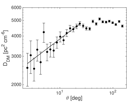
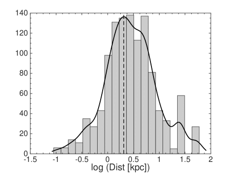
Figure 3.— (a) DM SF for $1141$ pulsars at $|\text{GB}|>5^{\circ}$. The solid line represents the fit to the data, which is described by Eq. (20). (b) The distribution of the pulsar distances. The kernel density estimation is shown by the thick solid line. The peak of the distribution is indicated by the vertical dashed line.

(2) The interstellar turbulence in the diffuse WIM with a Kolmogorov density spectrum ($|\text{GB}|>5^{\circ}$ and $120^{\circ}<\text{GL}<240^{\circ}$).

To probe the turbulence in the diffuse WIM, we choose the pulsars in an area of the sky with $|\text{GB}|>5^{\circ}$ and $120^{\circ}<\text{GL}<240^{\circ}$, which is off the Galactic midplane toward the outer Galaxy (see Fig. 1). Similar to the above analysis we present their DM SF in Fig. 4. The large error bars come from the small size of the subsample of pulsars used here. The fit to the data at small $\theta$ shows

$$D_{\text{DM}}(2.5^{\circ}<\theta<5.0^{\circ})[\text{pc}^{2}\text{cm}^{-6}]$$ (27)

$$= 52.1\pm 1.1\times 10^{2}(\theta[^{\circ}])^{1.58\pm 1.43}.$$

The corresponding range of length scales for the fit, i.e., $L\theta$, is $\approx 79$ pc$-157$ pc, where $L\approx 1.8$ kpc is taken as the peak of the distribution of the pulsar distances (see Fig. 4). Because of the lower density in the diffuse WIM, we see a lower level of DM fluctuations compared with the case in cold interstellar phases (see Eq. (20)). Based on the fitted power-law index, we find that Eq. (14b) in Case 2 applies to this situation. Under the consideration $R=L\theta$, Eq. (14b) can be rewritten as

$$D(\theta)\approx 2\langle\delta n_{e}^{2}\rangle L_{i}^{-m}(L+L_{i})L^{m+1}\theta^{m+1}$$

$$D(\theta)\approx +\frac{1}{3}\big{(}\langle\delta n_{e}^{2}\rangle+n_{e0}^{2}\big{)}(L-L_{i})^{2},~{}~{}~{}~{}~{}~{}~{}~{}~{}\theta\lesssim\frac{L_{i}}{L},$$ (28a)

$$D(\theta)\approx 2\langle\delta n_{e}^{2}\rangle L_{i}(L+L_{i})+\frac{1}{3}\big{(}\langle\delta n_{e}^{2}\rangle+n_{e0}^{2}\big{)}(L-L_{i})^{2},$$

$$D(\theta)\approx ~{}~{}~{}~{}~{}~{}~{}~{}~{}~{}~{}~{}~{}~{}~{}~{}~{}~{}~{}~{}~{}~{}~{}~{}~{}~{}~{}~{}~{}~{}~{}~{}~{}~{}~{}~{}~{}~{}~{}~{}~{}~{}~{}~{}~{}~{}~{}~{}~{}~{}~{}~{}~{}~{}~{}~{}\theta\gtrsim\frac{L_{i}}{L}.$$ (28b)

For a steep density spectrum, $L_{i}$ coincides with the energy injection scale of turbulence. It is believed to be in the range $\sim 50-500~{}$ pc in the ISM (Elmegreen & Scalo, 2004; Chepurnov et al., 2010; Beck et al., 2016), with the main driver as supernova explosions (Padoan et al., 2016). As $L_{i}$ is much less than $L$, we recast the above equation into

$$D(\theta)\approx 2\langle\delta n_{e}^{2}\rangle L_{i}^{-m}L^{m+2}\theta^{m+1}$$

$$D(\theta)\approx +\frac{1}{3}\big{(}\langle\delta n_{e}^{2}\rangle+n_{e0}^{2}\big{)}L^{2},~{}~{}~{}~{}~{}~{}~{}~{}~{}~{}~{}~{}\theta\lesssim\frac{L_{i}}{L},$$ (29a)

$$D(\theta)\approx 2\langle\delta n_{e}^{2}\rangle L_{i}L+\frac{1}{3}\big{(}\langle\delta n_{e}^{2}\rangle+n_{e0}^{2}\big{)}L^{2},$$

$$D(\theta)\approx ~{}~{}~{}~{}~{}~{}~{}~{}~{}~{}~{}~{}~{}~{}~{}~{}~{}~{}~{}~{}~{}~{}~{}~{}~{}~{}~{}~{}~{}~{}~{}~{}~{}~{}~{}~{}~{}~{}~{}~{}~{}~{}~{}~{}~{}~{}~{}~{}\theta\gtrsim\frac{L_{i}}{L}.$$ (29b)

The comparison between Eq. (29a) and Eq. (27) provides constraints on the parameters,

$$m=0.58,$$ (30a)

$$\Big{(}\frac{\langle\delta n_{e}^{2}\rangle}{2\times 10^{-4}~{}\text{cm}^{-6}}\Big{)}\Big{(}\frac{L_{i}}{100~{}\text{pc}}\Big{)}^{-0.58}\approx 4.5,$$ (30b)

$$\frac{1}{3}\big{(}\langle\delta n_{e}^{2}\rangle+n_{e0}^{2}\big{)}L^{2}<D_{\text{DM}}(\theta=2.5^{\circ}),$$ (30c)

where $L\approx 1.8$ kpc is used. Here Eq. (30c) gives

$$\sqrt{\langle\delta n_{e}^{2}\rangle+n_{e0}^{2}}<0.014~{}\text{cm}^{-3}.$$ (31)

The resulting spectral index $\alpha_{\text{3D}}=-m-3=-3.58$ (Eq. (3b)) is very close to the Kolmogorov slope. This is expected for the turbulence in the diffuse WIM (Armstrong et al., 1995; Chepurnov & Lazarian, 2010). Since the diffuse WIM is not preferentially populated by pulsars, the limited size of the sample and the contaminations from, e.g., H II regions, along the path prevent us from obtaining an extended density spectrum over many orders of magnitude in scales as the composite spectrum obtained from the scintillations and scattering of nearby pulsars in the local ISM (Armstrong et al., 1995).

As shown in Fig. 4, instead of saturating at large $\theta$, the SF exhibits another power law, which will be discussed below.

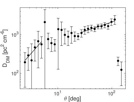
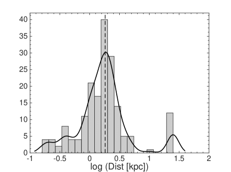
Figure 4.— Same as Fig. 3, but for $181$ pulsars at $|\text{GB}|>5^{\circ}$ and $120^{\circ}<\text{GL}<240^{\circ}$. The data points at small and large $\theta$ in (a) are separately fitted by Eq. (27) and Eq. (32), respectively.

(3) Galactic-scale turbulence with a steep density spectrum ($|\text{GB}|>10^{\circ}$).

In the above analysis, we find a separate power law at large $\theta$ in the WIM, which can be fitted by

$$D_{\text{DM}}(27.4^{\circ}<\theta<113.5^{\circ})[\text{pc}^{2}\text{cm}^{-6}]$$ (32)

$$= (2.4\pm 1.4)\times 10^{2}(\theta[^{\circ}])^{0.47\pm 0.14}.$$

A similar power law can also be found for a larger sample of pulsars that lie over the entire range of longitude but at higher latitudes. Fig. 5 displays the DM SF for the pulsars at $|\text{GB}|>10^{\circ}$. The SF at small $\theta$ is dominated by non-turbulent density structures in the inner Galaxy. At large $\theta$, it can be fitted by

$$D_{\text{DM}}(27.4^{\circ}<\theta<113.5^{\circ})[\text{pc}^{2}\text{cm}^{-6}]$$ (33)

$$= (5.1\pm 1.0)\times 10^{2}(\theta[^{\circ}])^{0.29\pm 0.05}.$$

We assume that the power-law behavior of the SF at large $\theta$ is also of turbulent origin. Based on the SF slope and the range of $\theta$, we find that it can be approximately treated as Case 3 in Section 2.

We rewrite Eq. (18c) by replacing $R$ with $L\theta$,

$$D(\theta)\approx 2\langle\delta n_{e}^{2}\rangle L_{i}^{-m}L^{m+2}\theta^{m+1}+\frac{1}{3}\big{(}\langle\delta n_{e}^{2}\rangle+n_{e0}^{2}\big{)}L^{2},$$

$$D(\theta)\approx ~{}~{}~{}~{}~{}~{}~{}~{}~{}~{}~{}~{}~{}~{}~{}~{}~{}~{}~{}~{}~{}~{}~{}~{}~{}~{}~{}~{}~{}~{}~{}~{}~{}~{}~{}~{}~{}~{}~{}~{}~{}~{}~{}~{}~{}~{}~{}~{}~{}~{}~{}~{}~{}~{}~{}~{}\theta\lesssim\frac{1}{2},$$ (34a)

$$D(\theta)\approx \langle\delta n_{e}^{2}\rangle L_{i}^{-m}L^{m+2}\theta^{m}+\frac{1}{3}\big{(}\langle\delta n_{e}^{2}\rangle+n_{e0}^{2}\big{)}L^{2},$$

$$D(\theta)\approx ~{}~{}~{}~{}~{}~{}~{}~{}~{}~{}~{}~{}~{}~{}~{}~{}~{}~{}~{}~{}~{}~{}~{}~{}~{}~{}~{}~{}~{}~{}~{}~{}~{}~{}~{}~{}~{}~{}~{}~{}~{}~{}~{}~{}~{}~{}\frac{1}{2}\lesssim\theta\lesssim\frac{L_{i}}{L},$$ (34b)

$$D(\theta)\approx \langle\delta n_{e}^{2}\rangle L^{2}+\frac{1}{3}\big{(}\langle\delta n_{e}^{2}\rangle+n_{e0}^{2}\big{)}L^{2},~{}~{}~{}\theta\gtrsim\frac{L_{i}}{L}.$$ (34c)

We adopt the fit in Eq. (33), as it is obtained from a larger sample size compared with Eq. (32). A comparison between Eq. (33) and Eq. (34b) yields

$$m=0.29,$$ (35a)

$$\Big{(}\frac{\langle\delta n_{e}^{2}\rangle}{10^{-4}~{}\text{cm}^{-6}}\Big{)}\Big{(}\frac{L_{i}}{2~{}\text{kpc}}\Big{)}^{-0.29}\approx 4.1,$$ (35b)

$$\frac{1}{3}\big{(}\langle\delta n_{e}^{2}\rangle+n_{e0}^{2}\big{)}L^{2}<D_{\text{DM}}(\theta=27.4^{\circ}),$$ (35c)

where Eq. (35c) implies

$$\sqrt{\langle\delta n_{e}^{2}\rangle+n_{e0}^{2}}<0.032~{}\text{cm}^{-3}.$$ (36)

Here we use $L\approx 2.0~{}$kpc as derived from the distribution of the pulsar distances (see Fig. 5). We note that the driving scale of turbulence $L_{i}$ is larger than $L$ (see Case 3 in Section 2), but appears to be of the same order of magnitude as $L$. This is consistent with the length scale $\approx 4.0$ kpc corresponding to $113.5^{\circ}$ where the SF reaches its maximum value. Over the range of length scales $\approx 956$ pc$-4.0$ kpc, which extends to scales larger than the scale height $\approx 1.7$ kpc of the thick disk in the YMW16 model (Yao et al., 2017), the 1D power-law index of the density spectrum is $\alpha_{\text{1D}}=-m-1=-1.29$. It is a bit shallower than the Kolmogorov slope ($-5/3$) as expected for 2D turbulence in the inverse cascade regime in a nearly incompressible medium (Kraichnan, 1967; Dastgeer & Zank, 2005). The expected steepening of SF at $\theta\lesssim 0.5$ radians, i.e., $\theta\lesssim 28.6^{\circ}$, in Eq. (34a) is not seen in Fig. 5 due to the presence of non-turbulent density structures on smaller length scales.

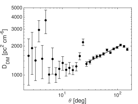
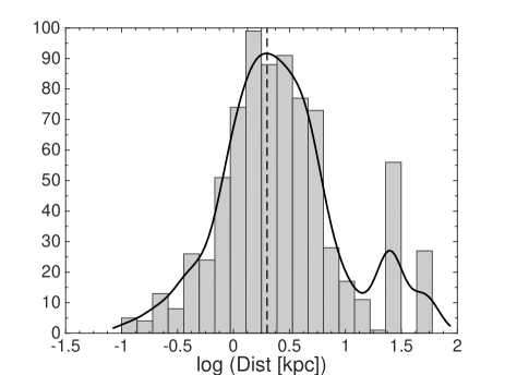
Figure 5.— Same as Fig. 3, but for $773$ pulsars at $|\text{GB}|>10^{\circ}$. The fit in (a) is given by Eq. (33).

The above Galactic-scale density spectrum can only been seen in the diffuse WIM. Its effect on shaping the density structures near the Galactic plane is insignificant (see Fig. 3). A flat Galactic magnetic energy spectrum with a 1D power-law index $-0.37$ over the range $0.5-15$ kpc was earlier measured by Han et al. (2004), based on the rotation and dispersion measures of pulsars. For external spiral galaxies, density and velocity power spectra extending to scales comparable to the size of galactic disk have also been reported (Dutta et al., 2013; Nandakumar & Dutta, 2020). Gravitational instabilities are believed to be the main driver of such galactic-scale turbulence, especially for the galaxies with relatively high star formation rates (Elmegreen et al., 2003; Romeo & Agertz, 2014; Krumholz & Burkhart, 2016). An inverse cascade in a quasi-2D disk can also contribute to the large-scale turbulence (Wada et al., 2002; Bournaud et al., 2010).

4. Discussion and conclusions

We summarize the density spectra obtained from the DM SF of pulsars in Table 1. They reveal different properties of turbulence depending on the interstellar phase and the range of length scales. Our results demonstrate that the DMs of pulsars bear unique signatures of interstellar turbulence and can be used synergistically with other statistical techniques to achieve a comprehensive picture of interstellar density structures and distribution.

Earlier models for the Galactic electron density distribution, e.g., the NE2001 model (Cordes & Lazio, 2002, 2003), the YMW16 model (Yao et al., 2017), include multiple components and involve a large number of parameters to account for the basic structure with thin and thick disks, spiral arms, and other local features. Differently, here we focus on the statistics of electron density fluctuations ($\delta n_{e}$ in Eq. (1)), which are only characterized by turbulence parameters and can be used to statistically explain the observations of a large number of pulsars (Xu & Zhang, 2017) and other turbulence-related observations (Xu & Zhang, 2016).

Table 1Electron density spectra in the ISM obtained from DMs of pulsars

Area of sky	Interstellar phase	Measured range of length scales	$\sqrt{\langle\delta n_{e}^{2}\rangle}$ [cm-3]	$L_{i}$	$\alpha_{\text{1D}}$
$|\text{GB}|>5^{\circ}$	Cold phases	$87$ pc$-831$ pc	$\sim 0.3$	$\sim$ pc (inner scale)	$-0.25$
$|\text{GB}|>5^{\circ}$ and $120^{\circ}<\text{GL}<240^{\circ}$	WIM	$79$ pc$-157$ pc	$\sim 0.01$	$\sim 100$ pc (outer scale)	$-1.58$
$|\text{GB}|>10^{\circ}$	WIM	$956$ pc$-4.0$ kpc	$\sim 0.01$	$4.0$ kpc (outer scale)	$-1.29$

Compared with the rotation measure SF and scatter broadening of pulsars, without contributions from magnetic fields or invoking the scattering effect, the DM SF of pulsars provides a relatively clean and direct measurement of density fluctuations over a range of length scales. Here we found a shallow density spectrum extending to larger scales compared with our earlier studies in Xu & Zhang (2016) and Xu & Zhang (2017). Its inner cutoff scale on the order of pc, which was also suggested by the rotation measure SF (Xu & Zhang, 2016), might be related to the phase transition and formation of molecular hydrogen. Within molecular clouds, the interstellar scattering is more suitable than the DM SF of pulsars to probe the sub-pc density fluctuations (Xu & Zhang, 2017). As shallow density spectra have also been measured with cold gas tracers both at high latitudes (e.g., Chepurnov et al. 2010) and in molecular clouds (Hennebelle & Falgarone, 2012), our methods can be used synergistically with cold gas tracers to probe the supersonic turbulence in cold interstellar phases.

Compared with the statistical measurement of density fluctuations using the diffuse H$\alpha$ emission, as pulsars are primarily distributed in the Galactic disk, they can be used to probe the cold gas phases at low latitudes (see above). However, the DMs of pulsars are sensitive to all density fluctuations along the lines of sight and thus are more subjected to non-turbulent “noises” than the high-latitude H$\alpha$ emission in measuring turbulent density spectra. It means that the DMs of pulsars are less favored than the diffuse H$\alpha$ emission to study the turbulence in the diffuse WIM. In addition, different from the statistical measurements using spatially continuous emission, when we use discrete point sources, the angular resolution is determined by the projected separation between two point sources and their distances from the observer. It determines the minimum length scale for the SF analysis of turbulent fluctuations. We note that the Kolmogorov density spectrum seen from the diffuse H$\alpha$ emission was also inferred from radio scattering observations of nearby pulsars on scales down to $10^{6}$ m (Armstrong et al., 1995), but this is only for the measurement of the local ISM, where the turbulence is not supersonic and the lines of sight do not pass through the non-turbulent density structures in the disk.

Besides the shallow density spectrum in cold phases and the Kolmogorov-like density spectrum in the diffuse WIM, we also found a steep density spectrum on very large scales, suggesting the existence of galactic-scale turbulence in the Milky Way similar to other external spiral galaxies. Its interaction with the smaller-scale interstellar turbulence and its role in e.g., gas dynamics and star formation deserves further investigation.

It is important to stress that different from the statistical measurements of turbulent velocities, density statistics do not directly show the dynamics and energy cascade of turbulence. They preferentially trace the compressive component of turbulence, which is responsible for generating large density contrasts. Therefore, the measured shallow density spectrum should not be treated as the evidence for the dominance of compressive component over solenoidal component of turbulence in the disk. The latter, in fact, can be dominant across most of the volume in cold cloud phases (Padoan et al., 2016; Qian et al., 2018; Xu, 2020).

References

- Armstrong et al. (1981) Armstrong, J. W., Cordes, J. M., & Rickett, B. J. 1981, Nature, 291, 561
- Armstrong et al. (1995) Armstrong, J. W., Rickett, B. J., & Spangler, S. R. 1995, ApJ, 443, 209
- Beck et al. (2016) Beck, M. C., Beck, A. M., Beck, R., Dolag, K., Strong, A. W., & Nielaba, P. 2016, J. Cosmol. Astropart. Phys., 2016, 056
- Beresnyak et al. (2005) Beresnyak, A., Lazarian, A., & Cho, J. 2005, ApJ, 624, L93
- Bournaud et al. (2010) Bournaud, F., Elmegreen, B. G., Teyssier, R., Block, D. L., & Puerari, I. 2010, MNRAS, 409, 1088
- Brandenburg & Lazarian (2013) Brandenburg, A., & Lazarian, A. 2013, Space Sci. Rev.
- Burkhart et al. (2009) Burkhart, B., Falceta-Gonçalves, D., Kowal, G., & Lazarian, A. 2009, ApJ, 693, 250
- Chepurnov & Lazarian (2010) Chepurnov, A., & Lazarian, A. 2010, ApJ, 710, 853
- Chepurnov et al. (2010) Chepurnov, A., Lazarian, A., Stanimirović, S., Heiles, C., & Peek, J. E. G. 2010, ApJ, 714, 1398
- Cordes & Lazio (2002) Cordes, J. M., & Lazio, T. J. W. 2002, arXiv:astro-ph/0207156
- Cordes & Lazio (2003) —. 2003, arXiv:astro-ph/0301598, astro
- Dastgeer & Zank (2005) Dastgeer, S., & Zank, G. P. 2005, Nonlinear Processes in Geophysics, 12, 139
- Dutta et al. (2013) Dutta, P., Begum, A., Bharadwaj, S., & Chengalur, J. N. 2013, NewA, 19, 89
- Elmegreen (1999) Elmegreen, B. 1999, in The Physics and Chemistry of the Interstellar Medium, ed. V. Ossenkopf, J. Stutzki, & G. Winnewisser, 77
- Elmegreen et al. (2003) Elmegreen, B. G., Elmegreen, D. M., & Leitner, S. N. 2003, ApJ, 590, 271
- Elmegreen et al. (2001) Elmegreen, B. G., Kim, S., & Staveley-Smith, L. 2001, ApJ, 548, 749
- Elmegreen & Scalo (2004) Elmegreen, B. G., & Scalo, J. 2004, ARA&A, 42, 211
- Federrath & Banerjee (2015) Federrath, C., & Banerjee, S. 2015, MNRAS, 448, 3297
- Federrath & Klessen (2012) Federrath, C., & Klessen, R. S. 2012, ApJ, 761, 156
- Gaensler et al. (2008) Gaensler, B. M., Madsen, G. J., Chatterjee, S., & Mao, S. A. 2008, PASA, 25, 184
- Gaensler et al. (2011) Gaensler, B. M., et al. 2011, Nature, 478, 214
- Haffner et al. (2003) Haffner, L. M., Reynolds, R. J., Tufte, S. L., Madsen, G. J., Jaehnig, K. P., & Percival, J. W. 2003, ApJS, 149, 405
- Haffner et al. (2010) Haffner, L. M., et al. 2010, in Astronomical Society of the Pacific Conference Series, Vol. 438, The Dynamic Interstellar Medium: A Celebration of the Canadian Galactic Plane Survey, ed. R. Kothes, T. L. Landecker, & A. G. Willis, 388
- Han et al. (2004) Han, J. L., Ferriere, K., & Manchester, R. N. 2004, ApJ, 610, 820
- Heiles & Troland (2003) Heiles, C., & Troland, T. H. 2003, ApJ, 586, 1067
- Hennebelle & Falgarone (2012) Hennebelle, P., & Falgarone, E. 2012, A&A Rev., 20, 55
- Kowal et al. (2007) Kowal, G., Lazarian, A., & Beresnyak, A. 2007, ApJ, 658, 423
- Kraichnan (1967) Kraichnan, R. H. 1967, Physics of Fluids, 10, 1417
- Krishnakumar et al. (2015) Krishnakumar, M. A., Mitra, D., Naidu, A., Joshi, B. C., & Manoharan, P. K. 2015, ApJ, 804, 23
- Kritsuk et al. (2017) Kritsuk, A. G., Ustyugov, S. D., & Norman, M. L. 2017, New Journal of Physics, 19, 065003
- Krumholz & Burkhart (2016) Krumholz, M. R., & Burkhart, B. 2016, MNRAS, 458, 1671
- Lazarian (2009) Lazarian, A. 2009, Space Science Reviews, 143, 357
- Lazarian & Pogosyan (2000) Lazarian, A., & Pogosyan, D. 2000, ApJ, 537, 720
- Lazarian & Pogosyan (2004) —. 2004, ApJ, 616, 943
- Lazarian & Pogosyan (2006) —. 2006, ApJ, 652, 1348
- Lazarian & Pogosyan (2016) —. 2016, ApJ, 818, 178
- Lee & Lee (2019) Lee, K. H., & Lee, L. C. 2019, Nature Astronomy, 3, 154
- Lee & Jokipii (1976) Lee, L. C., & Jokipii, J. R. 1976, ApJ, 206, 735
- Lithwick & Goldreich (2001) Lithwick, Y., & Goldreich, P. 2001, ApJ, 562, 279
- Mac Low & Klessen (2004) Mac Low, M.-M., & Klessen, R. S. 2004, Reviews of Modern Physics, 76, 125
- Manchester et al. (2005) Manchester, R. N., Hobbs, G. B., Teoh, A., & Hobbs, M. 2005, AJ, 129, 1993
- McKee & Ostriker (2007) McKee, C. F., & Ostriker, E. C. 2007, ARA&A, 45, 565
- Minter & Spangler (1996) Minter, A. H., & Spangler, S. R. 1996, ApJ, 458, 194
- Nandakumar & Dutta (2020) Nandakumar, M., & Dutta, P. 2020, MNRAS, 496, 1803
- Ocker et al. (2020) Ocker, S. K., Cordes, J. M., & Chatterjee, S. 2020, ApJ, 897, 124
- Padoan et al. (2001) Padoan, P., Kim, S., Goodman, A., & Staveley-Smith, L. 2001, ApJ, 555, L33
- Padoan & Nordlund (2002) Padoan, P., & Nordlund, Å. 2002, ApJ, 576, 870
- Padoan et al. (2016) Padoan, P., Pan, L., Haugbølle, T., & Nordlund, Å. 2016, ApJ, 822, 11
- Peterson & Webber (2002) Peterson, J. D., & Webber, W. R. 2002, ApJ, 575, 217
- Pingel et al. (2018) Pingel, N. M., Lee, M.-Y., Burkhart, B., & Stanimirović, S. 2018, ApJ, 856, 136
- Qian et al. (2018) Qian, L., Li, D., Gao, Y., Xu, H., & Pan, Z. 2018, ApJ, 864, 116
- Romeo & Agertz (2014) Romeo, A. B., & Agertz, O. 2014, MNRAS, 442, 1230
- Scalo & Elmegreen (2004) Scalo, J., & Elmegreen, B. G. 2004, ARA&A, 42, 275
- Spitzer (1978) Spitzer, L. 1978, Physical processes in the interstellar medium (New York: Wiley-Interscience)
- Wada et al. (2002) Wada, K., Meurer, G., & Norman, C. A. 2002, ApJ, 577, 197
- Xu (2020) Xu, S. 2020, MNRAS, 492, 1044
- Xu et al. (2019) Xu, S., Ji, S., & Lazarian, A. 2019, ApJ, 878, 157
- Xu & Zhang (2016) Xu, S., & Zhang, B. 2016, ApJ, 824, 113
- Xu & Zhang (2017) —. 2017, ApJ, 835, 2
- Xu & Zhang (2020) —. 2020, ApJ, 898, L48
- Yao et al. (2017) Yao, J. M., Manchester, R. N., & Wang, N. 2017, ApJ, 835, 29
- Zuckerman & Palmer (1974) Zuckerman, B., & Palmer, P. 1974, ARA&A, 12, 279