Reducing Neural Network Parameter Initialization Into an SMT Problem

Abstract

Training a neural network (NN) depends on multiple factors, including but not limited to the initial weights. In this paper, we focus on initializing deep NN parameters such that it performs better, comparing to random or zero initialization. We do this by reducing the process of initialization into an SMT solver. Previous works consider certain activation functions on small NNs, however the studied NN is a deep network with different activation functions. Our experiments show that the proposed approach for parameter initialization achieves better performance comparing to randomly initialized networks.

Introduction

Satisfiability is the problem of determining if a formula has a model. In our case, formula is a set of propositions consisting of the weight and bias values of the NN and model is the set of initial values for them. Note that the described model is different from the common NN models. Intuitively, each possible model can be viewed as specifying a possible world within which a well formed formula can be evaluated (Barwise 1977). Also, coming up with reasonable initial values for weights and biases of a NN is NP-complete (Judd 1990; Blum and Rivest 1992).

In this paper, we investigate the complexity of initializing parameters in a more complicated NN, with hidden layers, nonlinear activation functions, and on a complex task: classifying the hand written digits (MNIST). In this setting, initializing parameters is not an NP-complete problem anymore, but NP-hard. We tried to reduce our problem to have a framework that solves instances using an SMT-solver.

Approach

The NP-Hard problem we address answers the question: “Is it possible to learn parameters of a deep NN for an arbitrary task such that it performs better than some relatively high threshold compared to randomly initialized parameters?”. Deep learning algorithms involve optimization in many contexts. The input of the optimization problem is a dataset and an objective, and the output is a set of values for the weights.

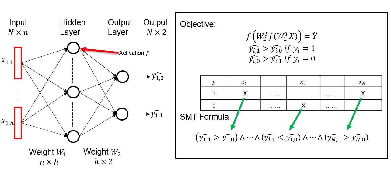
Figure 1: Overall framework. Left: schematic demonstration of a DNN; Right: the equivalent SMT formulation.

Traditionally, parameters are initialized to small random values, and are updated across many iterations by using an optimization algorithm. This algorithm mostly uses gradient computation to find optimal values of parameters minimizing or maximizing an objective function.

If the weights of a NN are initialized to all $0$s, then the activation of each node will be $0$ as well. They will also all compute the same gradients during backpropagation and undergo the exact same parameter updates. In other words, there is no source of asymmetry between neurons if their weights are initialized to have the same values.

Another approach is random initialization (Glorot and Bengio 2010). This way, weights are all random and unique in the beginning, so they compute distinct updates and integrate themselves as diverse parts of the full network. However, the problem is that there is no guarantee that model converges to an optimal weight assignment in a limited time frame. To converge faster, initialization of parameters is important. In this work, we investigate if SMT solvers could achieve a reasonable parameter initialization with a guarantee to better and faster convergence. First, the training process of a NN is reduced into an SMT problem for a binary classification problem. Second, the problem of integrating a non-linear activation function in an SMT solver and scalability of a large training set is investigated. Finally, the training results between randomly initialized weights and weights initialized by the results of an SMT solver are compared.

Reducing Training To SMT problem

NN Training

We are given a dataset composed of $N$ input vectors $\{x_{1},...,x_{N}\}$ of dimension $n$ and their respective labels $\{y_{1},...,y_{N}\}$. $X$ has the dimension of $n\times N$ where each column corresponds to an input $x_{i}$, and similarly, $Y$ is the label matrix of dimension $N\times 2$. Each label is a one-hot encoded vector where $1$ at index zero means the sample is from class $0$ and at index one means the sample is from class $1$.

An NN computes an estimation of a label given an input sample. Inference is done according to the value of the activation output after the final layer of the network. We define $h$ as the network function and $\theta$ as the set of network weights. For the input $x_{i}$, we have the estimated output $h(x_{i},\theta)=\hat{y}_{i}$ and the goal is to have $\hat{y}_{i}=y_{i}$. For a deep network composed of $k$ weights: $\theta=\{W_{1},...,W_{k}\}$ and for an activation function $f$, the output can be expressed as:

$$\hat{y}_{i}=h(x_{i};\theta)=f(W_{k}^{T}f(W_{k-1}^{T}f(...f(W_{1}^{T}x_{i})))$$ (1)

Having the predicted output and the ground truth, the following formula, called binary cross-entropy, is typically used as a loss function for classification tasks:

$$loss=-{(y\log(p)+(1-y)\log(1-p))}$$ (2)

where $p$ is the predicted probability of observed output and $y$ is a binary value indicating if the class label is correct.

Each weight has an arbitrary number of connections which define together the overall architecture of a deep NN. We call $\{h_{1},...,h_{k-1}\}$ the value of these hidden nodes, in definitive: $W_{1}\in\mathbb{R}^{n\times h_{1}}$, $W_{2}\in\mathbb{R}^{h_{1}\times h_{2}}$, …, $W_{k}\in\mathbb{R}^{h_{k-1}\times 1}$. Typically, a non-linear activation function $f$ is used to bring non-linearity in the NN function $h$. One of the most used functions is the ReLU function:

$$f(x)=\max(0,x)$$ (3)

The training is done in mini-batches of a certain size and is parameterized primarily in order to deal with large training datasets. The optimization algorithm is then used over many iterations organized in epochs to update the weights. It mostly consists of finding a local optima in the objective function and uses the backpropagation algorithm to compute the gradient of all parameters composing the network.

SMT Formula

Input of an SMT solver uses a set of variables representing real numbers that are expressed in classical order logic formula with equalities and/or inequalities, and translates it into a traditional $SAT$ formula. We want to express the task of NN with a formula where the input variables are the weights of the network. Since the weights represent the variables input to the SMT solver, we have in total $n\times h_{1}\times...\times h_{k-1}$ variables plus the corresponding bias terms.

To be consistent, we need the same settings given as input such as a training dataset, an architecture and a task. The architecture needs to be defined beforehand and will be integrated in the first-order logic formula. However, since we do not use the same algorithm for training as the classical approach, we do not use some hyper-parameter such as mini-batch size, learning-rate and number of training epochs.

We infer label $0$ if the first dimension of the output activation is higher than the second dimension as illustrated in Figure 1. We then express each clause of the SMT formulation as a part of the objective of the classification problem. The objective for one input $x_{i}$ is to have $\hat{y_{i}}=y_{i}$ which is expressed in as $\hat{y_{i,0}}>\hat{y_{i,1}}$ if $y_{i}=0$ and $\hat{y_{i,1}}>\hat{y_{i,0}}$ if $y_{i}=1$. A simplified version of the entire formula can be written as:

$$(\hat{y_{1}}=y_{1})\wedge...\wedge(\hat{y_{N}}=y_{N})$$ (4)

We notice that the length of the formula depends on the number of inputs provided in the training set. The more input samples are presented, the more constrained are the assignments of weights. This property links directly to the more traditional machine learning approach using gradient descent which highly rely on the number of training data.

We also noticed that putting all weights to zero can yield a satisfiable SMT formula depending if we use strict or loose inequalities. To avoid a dummy assignment of weights, another set of constraints added to enforce the values of the weights to be other than zero. We call $W_{ij}^{(k)}$, the value at the $i$th row and $j$th column of the weight at layer $k$. The formula then becomes:

The additional set of constraints is inspired from the dropout technique (Srivastava et al. 2014) used in NNs, where a layer sets a weight value to zero with a Bernoulli probability. In our case, we use the same method but instead we enforce random weight values to be different than zero.

One of the main components of NNs is the non-linear activation function. With that, it is possible to implement any function using NNs. To address this feature in the SMT formula, we set the activation function to ReLU (3).

References

- Barwise (1977) Barwise, J. 1977. An introduction to first-order logic. In Studies in Logic and the Foundations of Mathematics, volume 90, 5–46. Elsevier.
- Blum and Rivest (1992) Blum, A. L.; and Rivest, R. L. 1992. Training A 3-Node Neural Network Is NP-Complete.
- Glorot and Bengio (2010) Glorot, X.; and Bengio, Y. 2010. Understanding the difficulty of training deep feedforward neural networks. In In Proceedings of the International Conference on Artificial Intelligence and Statistics (AISTATS’10). Society for Artificial Intelligence and Statistics.
- Judd (1990) Judd, J. S. 1990. Neural Network Design and the Complexity of Learning. Cambridge, MA, USA: MIT Press. ISBN 0-262-10045-2.
- Srivastava et al. (2014) Srivastava, N.; Hinton, G.; Krizhevsky, A.; Sutskever, I.; and Salakhutdinov, R. 2014. Dropout: A Simple Way to Prevent Neural Networks from Overfitting. Journal of Machine Learning Research 15: 1929–1958. URL http://jmlr.org/papers/v15/srivastava14a.html.