Exploring the Galaxy’s halo and very metal-weak thick disk with SkyMapper and Gaia DR2

Abstract

In this work we combine spectroscopic information from the SkyMapper survey for Extremely Metal-Poor stars and astrometry from Gaia DR2 to investigate the kinematics of a sample of 475 stars with a metallicity range of $-6.5\leq\rm[Fe/H]\leq-2.05$ dex. Exploiting the action map, we identify 16 and 40 stars dynamically consistent with the Gaia Sausage and Gaia Sequoia accretion events, respectively. The most metal-poor of these candidates have metallicities of $\rm[Fe/H]=-3.31$ and $\rm[Fe/H]=-3.74$, respectively, helping to define the low-metallicity tail of the progenitors involved in the accretion events. We also find, consistent with other studies, that $\sim$21% of the sample have orbits that remain confined to within 3 kpc of the Galactic plane, i.e., |Z_max| $\leq$ 3 kpc. Of particular interest is a sub-sample ($\sim$11% of the total) of low |Z_max| stars with low eccentricities and prograde motions. The lowest metallicity of these stars has [Fe/H] = –4.30 and the sub-sample is best interpreted as the very low-metallicity tail of the metal-weak thick disk population. The low |Z_max|, low eccentricity stars with retrograde orbits are likely accreted, while the low |Z_max|, high eccentricity pro- and retrograde stars are plausibly associated with the Gaia Sausage system. We find that a small fraction of our sample ($\sim$4% of the total) is likely escaping from the Galaxy, and postulate that these stars have gained energy from gravitational interactions that occur when infalling dwarf galaxies are tidally disrupted.

1 Introduction

In the last decade, the astronomical community has experienced a renewal of interest in the properties of low-metallicity stars, particularly those with $\rm[Fe/H]<-2\,dex$. Motivated by the successful surveys of Beers et al. (1992) and Christlieb et al. (2008), in recent years numerous spectroscopic (e.g., SDSS, SEGUE, LAMOST, APOGEE; York et al., 2000; Yanny et al., 2009; Cui et al., 2012; Zhao et al., 2012; Majewski et al., 2017) and photometric (e.g., Pristine, SkyMapper; Starkenburg et al., 2017; Wolf et al., 2018) surveys have been commissioned, scanning extensive sky-areas for these very rare and key objects. We refer to Da Costa et al. (2019, their Section 1) for a more complete list of spectro-photometric surveys targeting low-metallicity stars. Not surprisingly, the underlying scientific motive is the understanding of the formation of our Galaxy, as well as other galaxies in the Universe.

Specifically, the lowest metallicity stars observable at the present-day formed from gas enriched with the nucleosynthetic products from first generation metal-free stars, the so-called Population-III stars. Studies of abundances and abundance ratios in ultra- and extremely metal-poor stars can then yield constraints on the properties of the Pop III stars, such as their masses, and on star formation processes at the earliest times (e.g., Frebel & Norris, 2015). Moreover, the kinematics of these stars can also provide much information on the events that occurred during the formation of the Milky Way (MW), which is believed to include both star formation in-situ and the accretion of lower-mass galaxies. Indeed, together the abundances and kinematics of the lowest metallicity stars offer a distinct perspective on the earliest stages of the formation and evolution of the Milky Way, and by implication, of galaxies in general.

In terms of the formation of the MW, the most common scenario predicts that the most metal-poor stars will be found mainly in the Galactic halo and Bulge, as these components likely formed in the earliest stages of the MW’s evolution (e.g. White & Springel, 2000; Brook et al., 2007; Tumlinson, 2010; El-Badry et al., 2018). In such a scenario relatively few, if any, very metal-poor stars are expected to lie in the MW disk as it formed at a later epoch after the settling into the plane of gas enriched by multiple generations of star formation (e.g. Bland-Hawthorn & Gerhard, 2016). However, recent kinematic results from surveys for the most metal-poor stars have cast doubt on this scenario, altering our understanding of the formation of the Milky Way. For example, the recent studies of Sestito et al. (2019, 2020b), Di Matteo et al. (2020) and Venn et al. (2020) have revealed a new scenario where $\sim\,20\,\%$ of very metal-poor stars have orbits that are confined to within 3 kpc of the MW plane; evidently the majority of these stars are not Galactic halo objects despite their low metallicities.

In particular, Sestito et al. (2019) compiled a catalogue of 42 ultra metal-poor ([Fe/H] $\leq$ –4.0) stars from the literature and analyzed their orbital properties making use of Gaia DR2 proper motions (Gaia Collaboration et al., 2018). They found that 11 out of 42 stars have prograde orbits that are confined to within 3 kpc of the Milky Way disk. Moreover, two of these MW-planar stars are found to be on nearly circular prograde orbits, and one is the star with the lowest overall metal content currently known (Caffau et al., 2011). In the same fashion, Di Matteo et al. (2020) investigated the kinematics of a sample of coincidentally the same number of low-metallicity stars drawn from the ESO Large Program “First stars – First nucleosynthesis” (Cayrel et al., 2004). Their analysis also finds that $\sim 20\%$ of the stars show disk-like kinematics. They went on to consider a larger sample of stars covering a wider metallicity range and found consistent results. Di Matteo et al. (2020) then postulated the existence of an “ultra-metal poor thick disk” that is an extension to low metallicities of the Galaxy’s thick disk population.

Sestito et al. (2020b) carried out a similar kinematic analysis on a substantially larger sample, consisting of 1027 very metal-poor stars with [Fe/H] $\leq$ –2.5 selected from the Pristine (Starkenburg et al., 2017; Aguado et al., 2019) and LAMOST (Cui et al., 2012; Li et al., 2018) surveys. Again they find that almost 1/3rd of the stars in the sample have orbits that do not deviate significantly from the disk plane of the Galaxy. They suggest that this implies that a significant fraction of the MW’s metal-poor stars formed with the Milky Way (thick) disk. Moreover, they note that as a consequence, the history of the disk must have been sufficiently quiescent that (presumably old) metal-poor stars were able to retain their disk-like orbits to the present-day (Sestito et al., 2020b).

Venn et al. (2020) have also investigated the kinematics of metal-poor stars using a sample of 115 objects chosen from the Pristine survey (Starkenburg et al., 2017) that have been observed at high dispersion. They find 16, out of 70, metal-poor stars whose orbits are confined to the vicinity of the Galactic plane, together with small numbers of stars that may have unbound orbits. They also identify stars whose orbital characteristics/actions are consistent with an origin in the Gaia Enceladus (Helmi et al., 2018) accretion event.

These somewhat unexpected results support the idea that the metallicity distribution of the Galaxy’s thick disk does indeed possess a low metallicity tail, as first advocated by Norris et al. (1985) and Morrison et al. (1990). Moreover, the proposed low metallicity tail would extend to lower metallicities than those authors suggested (see also Chiba & Beers, 2000; Beers et al., 2014).

The origin(s) of these metal-poor thick disk stars is, however, still uncertain, though the implications of their existence for the formation and evolution of the MW, and disk galaxies in general, are likely significant. A number of different possibilities have been discussed (e.g. Sestito et al., 2019, 2020b; Di Matteo et al., 2020) including that the stars were accreted from small satellites once the MW disk had already formed, or that they represent low metallicity stars formed in the gas-rich building-blocks that came together to form the main body of the Galaxy’s disk (see also the theoretical simulations presented in Sestito et al., 2020a).

In this work we conduct a similar study to those mentioned above by exploiting the metallicity determinations from the SkyMapper Survey for extremely metal-poor stars (see Da Costa et al., 2019), together with Gaia DR2 astrometry (Gaia Collaboration et al., 2018), to investigate the dynamics of 475 very metal-poor ([Fe/H] $<$ –2) stars in the southern sky. The wide extension in metallicity space, together with the relatively large number of stars, gives us a detailed view of the kinematic properties of these objects. We also consider the potential connection of any of the stars in our sample with the MW accretion events, such as those designated Gaia Enceladus, Gaia Sausage and Gaia Sequoia that have been recently discovered in large scale analyses of Gaia DR2 data (e.g. Helmi et al., 2018; Belokurov et al., 2018; Myeong et al., 2019; Mackereth et al., 2019). Such a connection has also been pursued in Monty et al. (2020).

The paper is organized as follows: in Sections 2 and 3 we present the data set and the orbit determination procedure, respectively, while in § 4 and § 5 we present and discuss our results. Specifically, in § 5.3 we discuss the small number of stars in our sample that appear not to be bound to the Galaxy. The final section (§ 6) summarizes our findings.

2 Data

The data set used in this work consists of 475 stars with metallicities ranging from $\rm[Fe/H]=-2.08$ to $\rm[Fe/H]<-6.5$ dex. It is composed as follows:

• 114 giant stars with $-6.2\leq\rm[Fe/H]_{1D,\,LTE}\leq-2.25$ dex. Of these stars 113 come from Yong et al. (in preparation), while the remaining star is the most-iron poor star for which iron has been detected: SMSS J160540.18–144323.1 with $\rm[Fe/H]_{1D,\,LTE}=-6.2\pm 0.2$ (Nordlander et al., 2019). These stars originate with the extremely metal-poor (EMP) candidates discussed in Da Costa et al. (2019) and all have been observed at high resolution, principally with the MIKE spectrograph (Bernstein et al., 2003) at the 6.5m Magellan (Clay) telescope. We shall refer to these stars as the HiRes data set.

• 45 stars observed with the FEROS high-resolution spectrograph (Kaufer et al., 1999) at the MPG/ESO 2.2-metre telescope at La Silla. Again, these stars originated from the Da Costa et al. (2019) sample. We removed from the analysis all the stars with $\rm[Fe/H]>-2$, and the stars in common with HiRes data set. The final count of stars belonging to this sub-sample is 38 and we label it as the FEROS data set.

• 122 stars from Jacobson et al. (2015) which have $-3.97\leq{\rm[Fe/H]}\leq-1.31$ dex. These stars originated in the SkyMapper commissioning-era survey (see Da Costa et al., 2019), and were also observed at high-dispersion with the MIKE spectrograph at Magellan. As for the FEROS sample, we removed 7 stars with $\rm[Fe/H]_{1D,\,LTE}>-2$ and the single star in common with the HiRes data set. However, as discussed in §3.2, there appears to be an issue with the radial velocities for the stars observed by Jacobson et al. (2015) during one specific Magellan/MIKE run, namely 2013 May 28 – June 01. As a result, we have removed the stars observed in that run that lack a radial velocity from Gaia DR2 and which had not been already discarded. The final sub-sample used here is then composed of 91 stars and we refer to it as the Jacobson+15 sub-sample.

• 17 stars from Marino et al. (2019) with metallicity $-3.26\rm<[Fe/H]_{1D,\,LTE}<-1.71$ dex. The spectra of these stars were obtained with the Keck HIRES high-resolution spectrograph (Vogt et al., 1994). After the removal of 2 stars present in the Jacobson+15 sub-sample, and 2 stars with $\rm[Fe/H]_{1D,\,LTE}>-2$, we retain 13 stars. This sub-sample is referred to as the Marino+19 data set.

• 362 giant star candidates from Da Costa et al. (2019) with either $\rm[Fe/H]_{\rm fitter}$$<-3.0$, or $-3.0\leq\rm[Fe/H]_{\rm fitter}\leq-2.5$ and $g_{\rm SkyMapper}<13.7$ mag. The radial velocities from the low-resolution spectra lack sufficient precision for our analysis, so the list of stars was cross-matched with Gaia DR2 to obtain radial velocities. A total of 195 stars were retained after the cross-match. These stars are referred to as the LowRes data set.

• 24 Ultra Metal-Poor giant stars $({\rm[Fe/H]}\leq-4)$ from Sestito et al. (2019), included to increase the number of UMP stars in the full sample and to provide a consistency check on our procedures. We have specifically selected only known giants from their sample for consistency with the SkyMapper derived samples, which are giant dominated. We refer to Sestito et al. (2019) for a detailed description of the data set but we note it includes the star SMSS J031300.36-670839.3, which has ${\rm[Fe/H]_{3D,NLTE}}<-6.5$ (Keller et al., 2014; Bessell et al., 2015; Nordlander et al., 2017). This data set is referred to as the Sestito+19 sub-sample.

Unless otherwise noted, the uncertainty in [Fe/H] values derived from high dispersion spectroscopy is taken as $\pm$0.10, while for the stars in the LowRes data set, the uncertainty is $\pm$0.3, and the values are quantized at 0.25 dex intervals. Figure 1 then shows the metallicity distribution of each data set, computed using kernel density estimation with a Gaussian kernel and a bandwidth parameter of 0.5; the number of stars belonging to each set is reported in the top-left corner of the panel. Each distribution has been normalized by the number of stars in the sample. Figure 1 also shows the distribution for the total sample formed by summing the individual distributions. As is apparent, the sample spans a wide range in metallicity, with a peak around $\rm[Fe/H]\sim-2.8$, consistent with the observed metallicity distribution function of the full SkyMapper EMP sample discussed in Da Costa et al. (2019).

Figure 1: Metallicity distributions of the data sets analysed in this work. The six different subsamples are marked with red, orange, blue, dark-red, navy and green. The metallicity distribution of the total sample is shown with the grey-black solid line. Each density distribution ($\phi$) has been computed with a Gaussian kernel and renormalized with the total number of stars in the sample for a correct relative visualization.

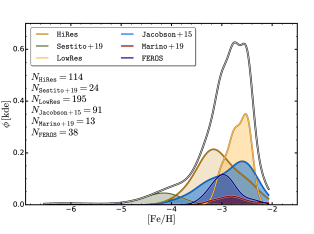
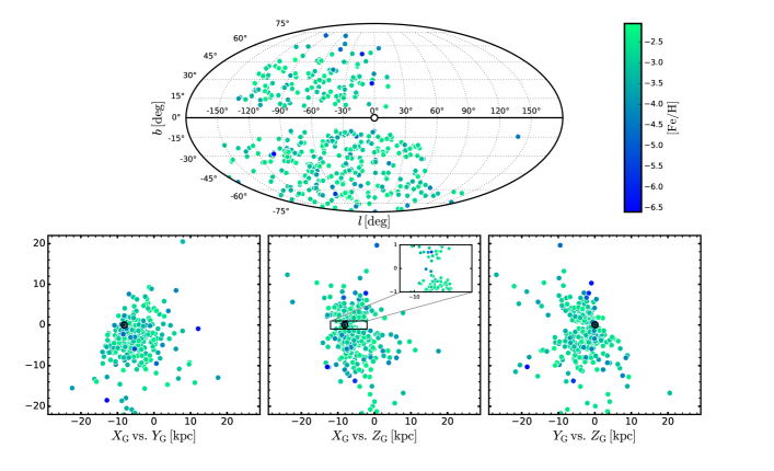
Figure 2 shows the position of the analyzed stars, both in Galactic latitude and longitude and in the Cartesian Galactocentric reference frame, with each star colour-coded according to its metallicity. Since $\sim\,90\%$ of the stars come from the SkyMapper survey, the data set is affected by the same selection biases as discussed in Da Costa et al. (2019). Specifically, the SkyMapper survey avoids regions of the sky with significant stellar crowding, while the selection process for candidates restricts the sample to stars with $E(B-V)<0.25$ mag. The net result is a lack of candidates near the Galactic plane and in the Galactic Bulge (see Figure 4 and Figure 14 in Da Costa et al., 2019) as is evident in the inset in the middle panel of Figure 2. Indeed, the majority of the stars lie inside the solar circle in the ($\rm{X}_{G},\rm{Y}_{G}$) plane, although at a variety of heights above and below the plane; the star nearest the Galactic Centre in the sample has a Galactocentric radius of $1.8\pm 0.8$ kpc.

Figure 2: Top panel. Mollweide projection of the analyzed stars in Galactic coordinates. Each star is colour coded according to its metallicity. Bottom panels. Position of the analyzed stars in the Galactocentric Cartesian reference frame using the derived distances as discussed in section 3.1. The inset in the middle-bottom panel shows a zoom of the Galactic plane region. In each panel the first named quantity is for the x-axis and the second is for the y-axis. The Sun, marked by the black circle, is at (–8.2, 0.0, 0.02) and the Galactic Centre is at the origin in this co-ordinate system.

3 Deriving the kinematics of the sample

To compute the orbit of a star the full 6-dimensional information for the position and velocity is needed. Specifically, we need right ascension ($\alpha$), declination ($\delta$), distance from the Sun (d), proper motions in right ascension and declination ($\mu_{\rm\alpha}\cos\delta,\mu_{\rm\delta}$), and the heliocentric radial velocity $(v_{\rm r}$). Gaia DR2 provides the optimal source for these parameters, noting that strictly Gaia provides a measurement of parallax, not distance, and that $v_{\rm r}$ is only available for the brightest stars. As recently discussed in Bailer-Jones et al. (2018), for example, simply inferring the distance from the parallax measurement alone can lead to unreliable results. To overcome this problem, Bailer-Jones et al. (2018) combined parallax measurements with a realistic prior for the distance as a function of Galactic longitude and latitude, to generate distance estimates.

Sestito et al. (2019) introduced an alternate approach to determining distances that combines the exquisite astrometry and photometry provided by Gaia DR2 with theoretical isochrones in a Bayesian analysis to infer the distance, as well as the physical properties surface gravity $(\log\,g)$ and effective temperature $(T_{\rm eff})$. An advantage of their technique is that it allows the breaking of the potential degeneracy between dwarf and giant star distances at a fixed $T_{\rm eff}$. In our case however, by deliberate choice of the colour-range used to define the underlying sample of low metallicity candidates in the SkyMapper EMP-survey (see Da Costa et al., 2019), our data set consists entirely of giants, so that any dwarf/giant distance ambiguity does not arise. It further allows us to exploit the effective temperatures and metallicities of our stars, which are known from either the high-resolution analyses or from the spectrophotometric fits to the low-resolution spectra, to derive absolute magnitudes via the use of red giant branch (RGB) isochrones, particularly for those stars that lack a reliable parallax determination. This approach has the underlying assumption that all the stars lie on the RGB, whereas the distribution of temperatures and gravities in Da Costa et al. (2019) suggests a small fraction (5–10%) of the total sample are red horizontal branch or early-AGB stars. Such stars are more luminous than RGB stars at the same effective temperature and thus the distance determinations based on the RGB locus will be smaller than the true distances. While this will result in some individually incorrect orbital parameters, the overall results are unaffected given the dominance of RGB stars in the sample.

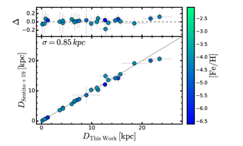
Details of our distance determinations are discussed in the next section, but when we compare our derived distances with those in Sestito et al. (2019) for the stars in common, we find excellent agreement. This is illustrated in Figure 3.

Figure 3: Lower panel: Comparison between the distance estimates in this work and those from Sestito et al. (2019). The solid line represents the 1:1 relation between the two different estimates. Upper panel: the relative differences between our distances and those from Sestito et al. (2019) expressed as $(\Delta=(D_{\rm TW}-D_{\rm S+19})/D_{\rm TW})$. The subscript TW indicates the values from this work. Each star is colour-coded according to its metallicity, as shown by the colour bar.

3.1 Distance determination

Our approach to determining distances for the stars in our sample is twofold. First, for the stars with unreliable Gaia DR2 parallax determinations, which we take here as those with $\sigma_{\rm\pi}/|\pi|\geq 0.15$, we adopted the following approach, which relies on the assumption that the stars in our sample, being very metal-poor, can be safely assumed to be old (age $\geq$ 10 Gyr). With this assumption we can then use the known $T_{\rm eff}$ and [Fe/H] values together with RGB isochrones of different metallicity to infer the absolute magnitudes and thus the distance. Specifically, we have used a set of Yonsei-Yale RGB isochrones ($Y^{2}$, Demarque et al. (2004)) for an age 12 Gyr, $[\alpha/{\rm Fe}]=+0.3$ and metallicities corresponding to [Fe/H] = –3.5, –2.5 and –1.9 to infer the V-band absolute magnitude $(M_{\rm V})$ for each star.

In practice, to find the absolute magnitude corresponding to a given star’s metallicity and $T_{\rm eff}$, we interpolated in $M_{\rm V}$ across the isochrones at the $T_{\rm eff}$ value. Since the isochrones use visual magnitudes, we first calculated the appropriate $V$ magnitude for each star from the Gaia $G$ values using the coefficients provided by the Gaia documentation. Reddening values from Schlegel et al. (1998) were adopted, corrected according to the recipe in Wolf et al. (2018). For stars with metallicities between $-4.5$ and $-3.5$, the $(M_{\rm V})$ value is a linear extrapolation, while for the small number of stars with [Fe/H] $\leq-4.5$, which come primarily from the Sestito et al. (2019) sub-sample, the $M_{\rm V}$ inferred for [Fe/H] = $-4.5$ was used. The uncertainties in the distances were then determined by assuming an uncertainty of $100\,\rm K$ in $T_{\rm eff}$ and $0.1\,\rm dex$ in metallicity ($0.3\,\rm dex$ for stars in LowRes subsample) and then propagating these values into the distance determination.

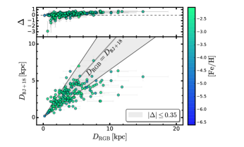
Second, for the stars with nominally reliable Gaia DR2 parallax determinations, i.e., those with $\sigma_{\rm\pi}/|\pi|<0.15$, we compared the Bailer-Jones et al. (2018) distances with the distances inferred from the RGB isochrones. This is shown in Fig. 4. While most stars do scatter about the 1:1 line, there are sizeable differences between the two estimates for $\sim$25% of the stars, most commonly with the RGB-based distance being larger than the Bailer-Jones et al. (2018) value, indicating that the parallax may have been overestimated, or that the RGB-based distance is incorrect.

We have not sought to investigate the origin of the discrepancy for each individual case, noting that we include uncertainties in $T_{\rm eff}$ and [Fe/H] when estimating the uncertainty in the RGB-based distance. There is, however, a potential systematic uncertainty introduced by RGB isochrone based approach. In particular, as discussed by Joyce & Chaboyer (2018), the location of theoretical RGBs in the Hertzsprung-Russell diagram is sensitive to the adopted value of the mixing length parameter $\alpha_{\rm MLT}$. The value of $\alpha_{\rm MLT}$ employed in any particular isochrone set (e.g., $\alpha_{\rm MLT}$ = 1.7 for the $Y^{2}$ isochrones) is usually determined by requiring a fit to the solar values, but, as demonstrated in Joyce & Chaboyer (2018), at low metallicities the location of the RGB computed with a solar-calibrated $\alpha_{\rm MLT}$ is more luminous by $\sim$0.3 mag at a fixed $T_{\rm eff}$ than a comparison with globular cluster RGB observations would suggest: a $\sim$10% smaller value of $\alpha_{\rm MLT}$ is required for consistency with the observations. It is possible therefore that our RGB-based distances are systematically over-estimated, though the comparison shown in Fig. 4 suggests that it is not a major effect.

In practice we have adopted the Bailer-Jones et al. (2018) distance and its uncertainty whenever the absolute value of the relative difference $(\Delta=\frac{D_{\rm RGB}-D_{\rm BJ+18}}{D_{\rm RGB}})$ is smaller than 0.35. This is shown as the grey shaded region in Figure 4. For the remainder, i.e., for the stars outside the shaded area with $|\Delta|>0.35$, we adopted the distance inferred from RGB isochrones. Overall, this results in the use of the RGB isochrone distance for 357 stars, while for the remaining 118 the Bailer-Jones et al. (2018) distance is employed.

The largest (heliocentric) distance of the stars in our sample is the RGB-based distance of $\sim 35$ kpc for the high-luminosity giant ($\log g$ $\approx$ 0.3) SMSS J004037.55–515025.1, which has [Fe/H] = –3.83 and is in the Jacobson+15 sub-sample. The smallest is the Bailer-Jones et al. (2018) distance of 0.21 kpc for the sub-giant BD+44 493 ($\log g$ $\approx$ 3.2 and [Fe/H] = –4.30) from the Sestito+19 sub-sample. Overall, the median heliocentric distance for the entire sample is $\sim 5$ kpc, with a median $\sim 7$ kpc for RGB-based distances, and a median of $\sim 3$ kpc for Bailer-Jones et al. (2018) distances.

Figure 4: Comparison between the distance determined in this work and the distance inferred in Bailer-Jones et al. (2018) for the 195 stars with $\sigma_{\pi}/|\pi|<0.15$. Each star is colour coded according to its metallicity, as shown in the right colour-bar. The grey shaded region within the black solid lines encloses stars with $|\Delta|\leq 0.35$, for which we adopted the Bailer-Jones distances. The top panel shows the relative differences between distances inferred through RGB isochrones and distances from Bailer-Jones et al. (2018) $(\Delta=(D_{\rm RGB}-D_{\rm BJ+18})/D_{\rm RGB})$

3.2 Orbital properties

To compute the orbital parameters we used the full 6-dimensional information on the position and velocity for each star. Gaia DR2 provides coordinates and proper motions, while the distances have been obtained as discussed in the previous section. Radial velocities come from the high-dispersion spectra, when available, and from Gaia DR2 for the LowRes sample.

We note that there are a number of the stars with radial velocities from the high-dispersion spectra that also have radial velocities from Gaia DR2, and this allows us to check for anything unusual or unexpected. As mentioned in §2, in this comparison process we discovered an anomaly in the Jacobson et al. (2015) radial velocities for a particular Magellan/MIKE run. In that run 32 stars were observed of which 8 also have radial velocities from Gaia DR2. The comparison for these 8 stars shows extreme disagreement for 7 stars, with values of the difference V_r(J+15) – V_r(Gaia DR2) ranging from –400 to +415 $\rm km\,s^{-1}$. We are at a loss to explain the origin of the disagreements and have consequently excluded from the analysis the stars from this run that lack Gaia DR2 radial velocities, while using the Gaia DR2 radial velocities in the kinematic calculations for the remaining 7 stars that have [Fe/H] $\leq$ –2.0 dex. We stress that such large disagreements are seen only for this one observing run in the Jacobson+15 sample, the radial velocities from other runs are very consistent with Gaia DR2 values when available. This is also the case for the stars in the HiRes and FEROS samples. Overall, for the 41 stars with radial velocities from our high-dispersion spectra and from Gaia DR2, the velocities agree well with a mean difference, in the sense of our velocities minus Gaia, of 1.7 $\rm km\,s^{-1}$ and a standard deviation of 5.5 $\rm km\,s^{-1}$. This agreement indicates that any systematic uncertainties in the radial velocity determinations are very minor compared to other contributors to uncertainties in the orbit determinations. We have always used the radial velocity and the corresponding uncertainty from the high dispersion spectra when available; the Gaia radial velocities and their uncertainties were utilized only when there was no alternative.

The kinematics of our sample of metal-poor stars have been determined using the GALPY Python package (Bovy, 2015). The orbit of each star was obtained by direct integration backward and forward in time for 2 Gyrs.This choice relies on the assumption that such a timescale is shorter than any significant variation in the Galactic potential

We adopted the potential identified as the best candidate among the ones studied in McMillan (2017). Briefly, it consists of an axisymmetric model with a bulge, thin, thick and gaseous disks, and a Navarro-Frenk-White (Navarro et al., 1996) dark matter halo. The heliocentric distances derived in the previous section have been converted to distances from the Galactic Centre (GC) in the GALPY routine, specifying the galactocentric position of the Sun as $(X,Y,Z)=(-8.21,0,0.0208)\,\rm kpc$, and its circular speed as $v_{0}=232.8\,\rm km\,s^{-1}$. Both quantities are taken from McMillan (2017).

For each star we determined the apogalacticon and perigalacticon $(D_{\rm apo},\,D_{\rm peri})$ of the orbit, the maximum vertical excursion from the Galactic plane $(Z_{\rm max})$, the eccentricity $\left(e=\frac{D_{\rm apo}-D_{\rm peri}}{D_{\rm apo}+D_{\rm peri}}\right)$, the energy $(E)$, the three actions $(J_{\rm R},\,J_{\rm\phi},\,J_{\rm Z})$ and the velocity components $U,\,V,\,W$ in the frame of the local standard of rest (LSR). As have others (e.g. Myeong et al., 2018), we emphasize that action space is the ideal plane in which to evaluate large samples of MW stars to identify and study possible sub-structures and debris from accretion events. The reason is that the actions are nearly conserved under the hypothesis that the potential is smoothly evolving (Binney & Spergel, 1984).

The uncertainties associated with the derived orbital parameters are determined by sampling the Probability Distribution Functions (PDFs) of the observed values. In particular, we drew 500 random realizations of the distance and velocity components and, for each realization, recomputed the orbital parameters assuming Gaussian distributions with means and dispersions equal to the observed values and their uncertainties. In particular, the uncertainties in the two proper motion components $(\mu_{\rm\alpha}\cos\delta,\,\mu_{\rm\delta})$ were drawn from a bivariate Gaussian taking into consideration the full covariance as defined in Equation 1, following the Gaia DR2 documentation.

$$cov=\begin{pmatrix}\sigma^{2}_{\rm\mu_{\rm\alpha}}&\sigma_{\rm\mu_{\rm\alpha}}\cdot\sigma_{\rm\mu_{\rm\delta}}\cdot corr(\mu_{\rm\alpha},\mu_{\rm\alpha})\\ \sigma_{\rm\mu_{\rm\alpha}}\cdot\sigma_{\rm\mu_{\rm\delta}}\cdot corr(\mu_{\rm\alpha},\mu_{\rm\alpha})&\sigma^{2}_{\rm\mu_{\rm\delta}}\end{pmatrix}$$ (1)

The uncertainties on the orbital parameters have then been determined by propagating the $16^{\rm th}$ and $84^{\rm th}$ percentiles of the resulting parameter distributions.

As examples, we consider the two most iron-poor stars known: SMSS J031300.36–670839.3 (Keller et al., 2014; Bessell et al., 2015) and SMSS J160540.18–144323.1 (Nordlander et al., 2019). For the former we find an “outer-halo” orbit with $e=0.70\pm 0.05\,,D_{\rm peri}=6.5\pm 2.0,\,D_{\rm apo}=36.6\pm 9.8$ and $|Z_{\rm max}|=34.2\pm 9.2~{}{\rm kpc}$. These parameters are in good agreement with those listed in Sestito et al. (2019). For the latter star, however, we determine an extreme “outer-halo” orbit that may in fact be unbound as the derived energy $E$ is close to zero. The inferred parameters are $e=0.93,\,D_{\rm peri}=6.5\pm 2.0,D_{\rm apo}\approx 423$ and $|Z_{\rm max}|\approx 327~{}{\rm kpc}$; the latter two quantities are quite uncertain.

As discussed in detail in §5.3, SMSS J160540.18–144323.1 is, in fact, one of a small number of stars (30 out of 475) for which we find apparent apogalacticon distances larger than the Milky Way virial radius, i.e., larger than $\sim$250 kpc. For such stars, a substantial fraction of the 500 random realizations resulted in unbound orbits (i.e., $D_{\rm apo}=\infty$), thus potentially biasing both the medians and the uncertainties derived from the orbital parameter distributions. The uncertainties for these specific stars are considered in more detail in §5.3.

As an independent check on the uncertainties and on the role of the adopted potential, we can compare our orbit parameters with those listed in Sestito et al. (2019, see their Table 4) for the 24 Ultra Metal-Poor stars in common. The agreement is generally excellent. Specifically, defining $\Delta$ as the difference between our values and those of Sestito et al. (2019) normalized by our values, then for the 24 stars we find median $\Delta$ values of 0.04, 0.03, 0.03 and 0.08 for $D_{\rm apo}$, $D_{\rm peri}$, $J_{\rm\phi}$ and $E$, respectively, noting that for the energy comparison we have taken into account the different solar energy used here to that in the Sestito et al. (2019) study.

4 Results

Figure 5: Orbital parameters for the stars with $D_{\rm apo}\leq$ 250 kpc. Panels a) and b): Vertical action $(J_{\rm Z}\,\rm[km\,s^{-1}])$ and energy $(E\,\rm[km^{2}\,s^{-2}])$ as a function of the azimuthal action (i.e. the vertical component of the angular momentum, $J_{\rm\phi}\,\rm[km\,s^{-1}]$). All quantities have been normalized by the solar values. The horizontal dashed-dotted line in panel a) indicates $J_{\rm Z}/J_{\rm Z,\odot}=1.25\times 10^{3}$. Panels c) and d): Maximum altitude from the MW plane $(|Z_{\rm max}|\,\rm[kpc])$ and eccentricity plotted as a function of the apogalactic $(D_{\rm apo}\,\rm[kpc])$ distance. Note that since $|Z_{\rm max}|$ cannot exceed $D_{\rm apo}$, the region above the 1:1 line in panel c) is forbidden. The horizontal dashed-dotted line in panel c) marks $Z_{\rm max}=3\,\rm kpc$. Panels e) and f): as for panels c) and d) but split by $|Z_{\rm max}|$. Panels g) and h): as for panels c) and d) but split by metallicity [Fe/H].

The physical properties and the computed orbital parameters of the first 10 stars are listed in Tables 1 and 2 while the complete tables are available with the online supplementary material. For Table 1 the columns are, respectively, an index number, the Gaia DR2 and SkyMapper or other IDs, the on-sky location in degrees, the parallax and its uncertainty from Gaia DR2, the adopted distance and its uncertainty, a flag indicating whether the distance is from the RGB isochrones (value=0), or from Bailer-Jones et al. (2018) (value=1), the proper motions from Gaia DR2 and their uncertainties, the heliocentric radial velocity and its uncertainty, $\log\,T_{\rm eff}$ and its uncertainty, the abundance [Fe/H], the reddening, and the data set from which the star originates. Similarly for Table 2, the columns are the index number (as for Table 1), the eccentricity and its uncertainty, the apo- and peri-galactic distances, the maximum deviation from the Galactic plane, the actions $(J_{\rm R},\,J_{\rm\phi},\,J_{\rm Z})$, the energy, and the $U$, $V$ and $W$ velocity components in the LSR frame.

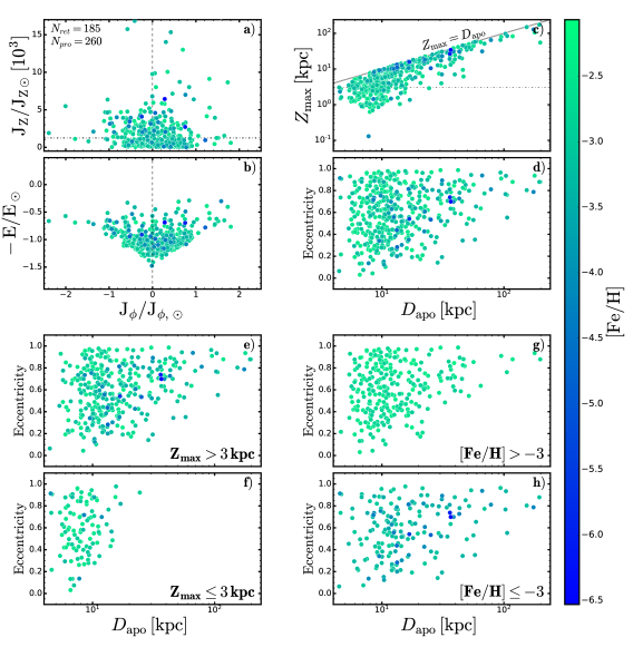
Figure 5 shows the inferred orbital parameters for all the stars with $D_{\rm apo}\leq$ 250 kpc, with each star colour-coded according to its metallicity, as shown in the right colour-bar. In particular, panels a) and b) show the vertical action $(J_{\rm Z}\,[\rm kpc\,\rm km\,s^{-1}])$, indicative of the vertical excursion of the star, and the orbital energy $(E\,\rm[km^{2}\,s^{-2}])$, as a function of the azimuthal action $(J_{\rm\phi}\,\rm[\rm kpc\,\rm km\,s^{-1}])$. The quantities have been normalized by the solar values computed for the McMillan2017 potential employed here: $J_{\rm\phi,\odot}=2014.24\,\rm kpc\,\rm km\,s^{-1}$, $J_{\rm Z,\odot}=0.302\,\rm\rm kpc\,\rm km\,s^{-1}$ and $E_{\rm\odot}=-153507.15\,\rm km^{2}\,s^{-2}$. We note that if we adopt the MWPotential2014 employed by Sestito et al. (2019), and include the increased dark matter halo mass, we obtain solar values similar to those in that work. Retrograde orbits are characterised by a negative value of $J_{\rm\phi}$, while prograde orbits have a positive $J_{\rm\phi}$. We find that overall $\sim 42\%\,(185/445)$ of our stars with $D_{\rm apo}\leq$ 250 kpc exhibit retrograde orbits, and note that the selection of the stars for inclusion in our sample should not have any bias as regards prograde or retrograde orbits.

Regarding the uncertainties in the derived orbital quantities, these are listed for each individual star in Table 2, but as examples, we find that for stars with $D_{\rm apo}\leq$ 20 kpc, the median errors in $D_{\rm apo}$, $D_{\rm peri}$, $|Z_{\rm max}|$ and $e$ are 0.9 kpc, 0.6 kpc, 1.0 kpc and 0.08, respectively. These increase to 11.6 kpc, 1.7 kpc, 7.7 kpc and 0.08 for stars with $20\leq D_{\rm apo}\leq$ 50 kpc, respectively, and to 56.4 kpc, 2.7 kpc, 52.0 kpc and 0.09 for stars with $50\leq D_{\rm apo}\leq$ 250 kpc.

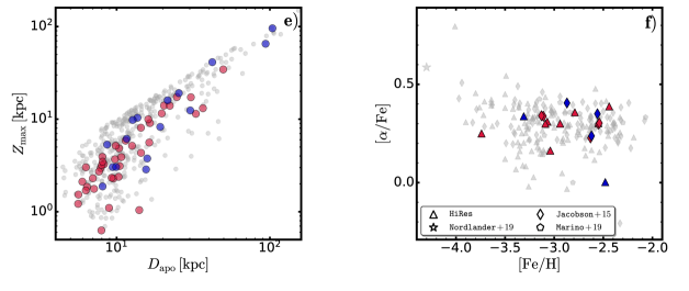
In panels c) and d) we show the maximum height $(|Z_{\rm max}|\,\rm[kpc])$ and eccentricity $e$ as function of the apogalatic distance $(D_{\rm apo}\,\rm[kpc])$. A preliminary inspection of panels a) and c) reveals that, despite the low metallicity of the stars in the sample, we detect a significant number of stars with small vertical excursion, in agreement with Sestito et al. (2019, 2020b) and Di Matteo et al. (2020). In particular, if we follow Sestito et al. (2020b) and adopt $J_{\rm Z}/J_{Zsun}<1.25\times 10^{3}$, shown as the dotted horizontal line in panel a), to characterize orbits that are confined to the disk, then $\sim$50% of our sample meets this definition. Similarly, if we follow Sestito et al. (2019) in using $|Z_{\rm max}|$ = $3\,\rm kpc$ (horizontal dashed-dotted line in panel c) of Figure 5) to discriminate between “disk-like” and “halo-like” orbits, we find that 102, or $\sim$21%, of the stars in our sample meet this criterion, i.e., have orbits that do not deviate far from the Galactic plane. Further, panel d) suggests that, while stars with $D_{\rm apo}\lesssim 25\,\rm kpc$ have an approximately uniform distribution in eccentricity, highly eccentric ($e\gtrsim 0.5$) orbits are favoured for stars with $D_{\rm apo}\gtrsim 25\,\rm kpc$, while panels c) and f) show that there is an apparent dearth of stars with low values of $|Z_{\rm max}|$ beyond $D_{\rm apo}$ $\approx$ 30 kpc. These apparent effects are most probably a consequence of the criteria adopted to select SkyMapper EMP candidates, as stars with low $|Z_{\rm max}|$ and large $D_{\rm apo}$ aren’t likely to meet the apparent magnitude cut that underlies the sample ($g_{\rm skymapper}<16$ for the HiRes stars and $g_{\rm skymapper}<13.7$ for the LowRes stars). In particular, the bottom-middle and bottom-right panels of Figure 2 show that stars with $|Z|$ $\leq$ 3 kpc and Galactocentric distances beyond 10-15 kpc are rare in our sample.

The two bottom left panels again show the eccentricity versus the apogalactic distance, but separately for stars with $|Z_{\rm max}|$ in excess of 3 kpc (panel e) and those with $|Z_{\rm max}|$ less than this value (panel f). Similarly, the two bottom right panels also show eccentricity versus the apogalactic distance but this time the sample is split by metallicity: stars with $\rm[Fe/H]>-3$ are shown in panel g) while the more metal-poor stars are shown in panel h). The similarity of panels g) and h) show that there is no obvious dependence of the kinematics on metallicity, at least for this sample of metal-poor stars.

Figure 6: [Fe/H] vs. $e$ for the stars with $D_{\rm apo}<250\,\rm kpc$. Gaia Sausage and Gaia Sequoia candidates are shown with blue and red circles, respectively. The Keller star (Keller et al., 2014; Nordlander et al., 2017) is shown as a grey star indicating the upper limit on the abundance.

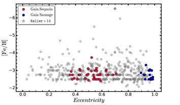
To more clearly illustrate this point, we show in Figure 6 a plot of [Fe/H] against $e$, the orbital eccentricity. Diagrams of this nature have long played an important role in discussions of the formation of the Galaxy. For example, in their classic paper, Eggen et al. (1962) argued on the basis of an apparent correlation between ultra-violet excess (an indicator of [Fe/H]) and orbital eccentricity, that the proto-Galaxy collapsed rapidly to a planar structure with a timescale of only a few $\times 10^{8}$ years. Specifically, in their sample of stars, those with [Fe/H] less than –1.5, approximately, all had $e\geq 0.6$ (Eggen et al., 1962). Norris et al. (1985) challenged the rapid collapse interpretation arguing that the lack of low-$e$ metal-poor stars was a result of a kinematic bias in the selection of the Eggen et al. (1962) sample. Instead, using a sample selected without any kinematic bias, Norris et al. (1985) showed that metal-poor stars with relatively low orbital eccentricities exist, a population they identified as a metal-weak component of the thick-disk. The Norris et al. (1985) result was confirmed and strengthened by Beers et al. (2014, see their Fig. 10) who showed that for stars with [Fe/H] $\leq$ –1.5 there is no correlation between orbital eccentricity and metallicity: stars can be found with $e$ values between $\sim$0.1 and 1. Our results in Figure 6 extend the lack of any correlation to substantially lower metallicities than those in Beers et al. (2014), where there were only a few stars at or below [Fe/H] = –2.5 and none below –3.0 dex. We discuss the implications of the existence of extremely metal-poor stars with low eccentricities (and low $|Z_{\rm max}|$) in §5.2. Figure 6 also shows the location of candidate members of the Gaia Sausage and Gaia Sequoia accretion events. The identification and properties of these stars are discussed in detail in §5.1.

Finally, as noted above, we find that 30 stars from the full sample have apparent $D_{\rm apo}$ values larger than 250 kpc, i.e., larger than the virial radius of the Milky Way. The majority of these stars possess energies that are consistent with, or larger than, zero and they likely have unbound orbits. These stars will be discussed in more detail in §5.3 but we note again that they are not plotted in the panels of Fig. 5 or in Fig. 6.

Table 1: Observed properties of the first ten stars in our sample. The columns are: a numeral index, Gaia DR2 and SkyMapper or other IDs, coordinates, parallax and uncertainty, distance and uncertainty, a flag for distance method (0=RGB interpolation, 1=Bailer-Jones et al. (2018)), proper motions and uncertainties, radial velocity and uncertainty, $\log T_{\rm eff}$ and uncertainty, [Fe/H], E(B-V) and origin data set as discussed in Section 2. The complete table is available electronically.

Index Gaia DR2 SMSS J $\alpha$ $\delta$ $\pi$ $\sigma_{\rm\pi}$ $D$ $\sigma_{\rm D}$ FLAG $\mu_{\rm\alpha}$ $\mu_{\rm\delta}$ $\sigma_{\rm\mu_{\rm\alpha}}$ $\sigma_{\rm\mu_{\rm\delta}}$ $v_{\rm r}$ $\sigma_{\rm v_{\rm r}}$ $log\,T_{\rm eff}$ $\sigma_{\rm log\,T_{\rm eff}}$ $\rm[Fe/H]$ $\rm E(B-V)$ $\rm Dataset_{\rm id}$ $\rm deg$ $\rm deg$ $\rm mas$ $\rm mas$ $\rm kpc$ $\rm kpc$ $\rm mas/yr$ $\rm mas/yr$ $\rm mas/yr$ $\rm mas/yr$ $\rm km\,s^{-1}$ $\rm km\,s^{-1}$ $\rm K$ $\rm K$ $\rm dex$ mag 1 2398202677437168384 230525.31-213807.0 346.3555462 -21.6353089 0.272750 0.049314 2.46 0.65 0 -1.142 -15.056 0.066 0.067 -15.7 0.4 3.708 0.009 -3.26 0.027 HiRes 2 2406023396270909440 232121.57-160505.4 350.3399235 -16.0848819 0.418462 0.036657 1.10 0.20 0 17.161 3.631 0.069 0.054 -39.1 1.0 3.736 0.008 -2.87 0.022 HiRes 3 2541284393302759296 001604.23-024105.0 4.0177235 -2.6848020 0.282214 0.046544 2.98 0.78 0 13.561 -9.876 0.093 0.055 49.3 1.2 3.705 0.009 -3.14 0.031 HiRes 4 2623363791014198656 224145.62-064643.0 340.4401074 -6.7786758 0.030874 0.031151 12.07 3.06 0 1.853 -2.861 0.053 0.048 -201.6 5.0 3.681 0.009 -3.16 0.029 HiRes 5 2666382767566459264 214716.16-081546.9 326.8173947 -8.2630725 0.499372 0.031415 3.48 0.93 0 1.497 -37.651 0.057 0.049 -12.3 0.3 3.708 0.009 -3.17 0.037 HiRes 6 2909324470226028800 053721.56-244251.5 84.3398617 -24.7143189 0.016537 0.027294 9.91 2.69 0 2.367 0.329 0.036 0.047 231.2 5.8 3.710 0.008 -3.50 0.021 HiRes 7 3064362275530429312 081627.99-055913.3 124.1166115 -5.9870501 0.176978 0.028682 7.47 1.92 0 -0.403 -1.921 0.048 0.032 159.8 4.0 3.688 0.009 -3.37 0.063 HiRes 8 3064545859613457536 081112.13-054237.7 122.8005492 -5.7104991 0.098921 0.047035 21.76 5.71 0 0.245 -2.879 0.075 0.066 121.0 3.0 3.686 0.009 -3.74 0.038 HiRes 9 3458991567268745728 120218.07-400934.9 180.5752523 -40.1597114 0.266276 0.035374 3.29 0.39 1 11.765 -2.682 0.040 0.029 -17.6 0.4 3.746 0.008 -2.89 0.090 HiRes 10 3473880535256883328 120638.24-291441.1 181.6593108 -29.2447637 0.257289 0.024364 3.41 0.28 1 -0.576 -2.246 0.031 0.016 58.1 1.5 3.708 0.009 -3.06 0.052 HiRes

Table 2: Derived orbital properties for the first ten stars in our sample. The columns are: numeral index; eccentricity; apo- and peri-perigalacticon distances; maximum height; orbital actions; orbital energy; $U$, $V$, $W$ velocities and orbit type (Halo, Disk, Sequoia, Sausage, Unbound). Each numerical quantity is followed by upper and lower uncertainties. The complete table is available electronically.

index $\rm Eccentricity$ $D_{\rm apo}$ $D_{\rm peri}$ $Z_{\rm max}$ $J_{\rm R}$ $J_{\rm\phi}$ $J_{\rm Z}$ $\rm Energy$ $U$ $V$ $W$ Orbit type $\rm kpc$ $\rm kpc$ $\rm kpc$ $\rm kpc\cdot km\,s^{-1}$ $\rm kpc\cdot km\,s^{-1}$ $\rm kpc\cdot km\,s^{-1}$ $\rm kpc\cdot km^{2}\,s^{-2}$ $\rm km\,s^{-1}$ $\rm km\,s^{-1}$ $\rm km\,s^{-1}$ 1 0.58 ${}_{-0.20}^{+0.17}$ 8.4 ${}_{-0.2}^{+0.3}$ 2.2 ${}_{-0.9}^{+1.4}$ 2.4 ${}_{-0.8}^{+1.0}$ 295.5 ${}_{-138.6}^{+137.9}$ 690.9 ${}_{-287.7}^{+360.1}$ 96.8 ${}_{-45.0}^{+55.2}$ -176530 ${}_{-634}^{+2662}$ 86.7 ${}_{-25.4}^{+22.1}$ -147.8 ${}_{-42.4}^{+48.3}$ 3.9 ${}_{-4.8}^{+5.6}$ Disk 2 0.28 ${}_{-0.06}^{+0.05}$ 10.4 ${}_{-0.6}^{+0.5}$ 5.9 ${}_{-0.3}^{+0.5}$ 1.4 ${}_{-0.3}^{+0.3}$ 104.6 ${}_{-43.7}^{+44.7}$ 1698.7 ${}_{-44.4}^{+51.1}$ 33.6 ${}_{-8.9}^{+9.0}$ -156666 ${}_{-697}^{+938}$ -83.8 ${}_{-15.6}^{+19.3}$ -16.0 ${}_{-2.8}^{+3.4}$ 16.6 ${}_{-4.9}^{+6.0}$ Disk 3 0.71 ${}_{-0.28}^{+0.17}$ 11.2 ${}_{-1.3}^{+1.7}$ 1.9 ${}_{-1.1}^{+2.0}$ 6.3 ${}_{-2.6}^{+2.7}$ 540.3 ${}_{-319.5}^{+227.7}$ 456.2 ${}_{-522.2}^{+582.2}$ 298.2 ${}_{-128.8}^{+127.1}$ -162656 ${}_{-2240}^{+6212}$ -91.6 ${}_{-26.4}^{+30.5}$ -165.6 ${}_{-52.5}^{+62.1}$ -121.1 ${}_{-22.9}^{+25.5}$ Halo 4 0.57 ${}_{-0.08}^{+0.12}$ 12.7 ${}_{-2.0}^{+3.0}$ 3.5 ${}_{-1.1}^{+1.2}$ 10.8 ${}_{-0.5}^{+1.8}$ 460.7 ${}_{-87.2}^{+84.5}$ -494.8 ${}_{-292.1}^{+319.1}$ 715.3 ${}_{-79.9}^{+204.8}$ -154330 ${}_{-7291}^{+10450}$ -63.8 ${}_{-6.4}^{+4.9}$ -253.2 ${}_{-44.3}^{+39.1}$ 58.4 ${}_{-33.3}^{+28.2}$ Halo 5 0.80 ${}_{-0.17}^{+0.14}$ 51.8 ${}_{-23.2}^{+98.8}$ 5.8 ${}_{-2.5}^{+0.4}$ 41.0 ${}_{-18.7}^{+81.7}$ 2937.5 ${}_{-2646.9}^{+19134394.1}$ -1367.7 ${}_{-431.8}^{+748.7}$ 1187.9 ${}_{-563.7}^{+661.6}$ -92378 ${}_{-63565}^{+86287}$ 245.3 ${}_{-75.1}^{+65.1}$ -515.5 ${}_{-141.5}^{+163.7}$ -225.7 ${}_{-66.0}^{+75.8}$ Halo 6 0.64 ${}_{-0.03}^{+0.02}$ 18.8 ${}_{-2.9}^{+3.4}$ 4.1 ${}_{-0.6}^{+1.2}$ 5.8 ${}_{-2.7}^{+6.4}$ 764.6 ${}_{-104.6}^{+72.7}$ 1488.5 ${}_{-186.2}^{+149.5}$ 153.8 ${}_{-78.2}^{+311.1}$ -136232 ${}_{-8547}^{+9007}$ -141.8 ${}_{-5.4}^{+6.1}$ -194.3 ${}_{-16.7}^{+16.4}$ 2.2 ${}_{-28.1}^{+31.7}$ Halo 7 0.57 ${}_{-0.05}^{+0.06}$ 14.3 ${}_{-1.6}^{+1.8}$ 4.0 ${}_{-0.2}^{+0.1}$ 2.1 ${}_{-0.4}^{+0.7}$ 489.9 ${}_{-109.4}^{+151.6}$ 1451.1 ${}_{-42.1}^{+39.9}$ 35.8 ${}_{-4.3}^{+9.8}$ -148391 ${}_{-5055}^{+4764}$ -60.9 ${}_{-8.8}^{+8.3}$ -146.4 ${}_{-12.2}^{+10.6}$ 6.0 ${}_{-12.8}^{+11.8}$ Disk 8 0.52 ${}_{-0.24}^{+0.30}$ 30.5 ${}_{-7.4}^{+13.4}$ 9.6 ${}_{-6.9}^{+14.8}$ 17.2 ${}_{-6.0}^{+6.5}$ 882.5 ${}_{-462.6}^{+568.7}$ -2744.0 ${}_{-3106.5}^{+2195.0}$ 632.8 ${}_{-383.4}^{+453.9}$ -110197 ${}_{-18420}^{+23747}$ 109.1 ${}_{-49.6}^{+50.3}$ -280.2 ${}_{-58.2}^{+56.9}$ -84.2 ${}_{-37.4}^{+33.3}$ Sequoia 9 0.76 ${}_{-0.06}^{+0.06}$ 30.7 ${}_{-4.4}^{+6.1}$ 4.1 ${}_{-0.5}^{+0.4}$ 4.0 ${}_{-1.3}^{+2.1}$ 1649.8 ${}_{-404.9}^{+566.7}$ 1830.3 ${}_{-125.6}^{+96.3}$ 55.5 ${}_{-12.8}^{+17.5}$ -114866 ${}_{-6481}^{+7743}$ 178.5 ${}_{-20.3}^{+22.7}$ 99.1 ${}_{-8.6}^{+9.3}$ -2.5 ${}_{-0.7}^{+0.7}$ Halo 10 0.38 ${}_{-0.02}^{+0.03}$ 9.1 ${}_{-0.1}^{+0.1}$ 4.1 ${}_{-0.2}^{+0.2}$ 2.4 ${}_{-0.2}^{+0.2}$ 159.9 ${}_{-17.4}^{+20.5}$ 1198.2 ${}_{-45.3}^{+38.8}$ 82.4 ${}_{-9.5}^{+11.6}$ -166959 ${}_{-216}^{+229}$ 34.7 ${}_{-0.7}^{+1.0}$ -52.8 ${}_{-2.3}^{+2.1}$ 7.0 ${}_{-3.0}^{+2.9}$ Disk

5 Discussion

In the following sub-sections we discuss in detail the results for the 475 very metal-poor stars analyzed. We will focus specifically on three key aspects. The first is the relation between the stars in our sample and the recently described remnants of the postulated Gaia Sequoia and Gaia Sausage accretion events (Belokurov et al., 2018; Myeong et al., 2019). For the sake of this analysis, following the hypothesis of Belokurov et al. (2018) and Myeong et al. (2019), we assume that these accretion events are distinct, but see Helmi et al. (2018) for an alternative view, particularly of Gaia Enceladus as a single ancient major merger event. The purpose of our work, however, is not to discern between the scenarios proposed to explain these structures in the Galactic halo, but rather to investigate their very low-metallicity content. The second key point is the analysis of low-metallicity stars with disk-like orbital properties that likely have a fundamental role in contributing to the understanding of the formation and evolution the MW’s disk. Finally, we discuss the properties and potential origin of the stars in our sample that are either loosely bound or not bound to the Galaxy.

5.1 Gaia Sausage and Gaia Sequoia candidate members

The exquisite data provided by Gaia DR2 has recently revealed the trace of at least two early major accretion events in the history of our Galaxy, referred to as Gaia Sausage and Gaia Sequoia (Helmi et al., 2018; Belokurov et al., 2018; Mackereth et al., 2019; Myeong et al., 2019; Koppelman et al., 2019). These discoveries are a direct consequence of the development of computational techniques and resources capable of processing very large data sets.

Here we exploit the action-space classification provided in Myeong et al. (2019, their Figure 9) to identify possible members of these accretion features within our sample of low-metallicity stars. Monty et al. (2020) have adopted a similar approach finding possible members of these systems with metallicities as low as $\rm[Fe/H]=-3.6$ dex. The number, abundances and abundance ratios of these stars could provide important information on the early evolution of the progenitors of the two accretion events.

The top-left panel of Figure 7 shows the action map $(J_{\rm Z}-J_{\rm R})/J_{\rm tot}$ vs. $J_{\rm\phi}/J_{\rm tot}$ with $J_{\rm tot}$ being the sum of the absolute value of the three actions $(J_{\rm tot}=J_{\rm R}+J_{\rm Z}+|J_{\rm\phi}|)$. Following the classification in Myeong et al. (2019), we highlight the loci of the Sequoia and Sausage accretion events with red and blue rectangles, respectively.

Figure 7: Panel a) Action map for all the stars in our sample. The red and blue boxes identify the Gaia Sequoia and Gaia Sausage loci, as determined in Myeong et al. (2019). Each star is colour coded according to its eccentricity. Panel b) Energy $(E)$ against azimuthal action $(J_{\rm\phi})$ normalized by the solar values. Red and blue circles represent Sequoia and Sausage candidate members, respectively, while grey small points mark stars outside of the selection boxes in the action map. Panel c) and d) Vertical action $(J_{\rm Z})$ against radial action $(J_{\rm R})$ and Toomre diagram, respectively. The solid lines in panel d) show circular velocities of 100 and 239 $\rm km\,s^{-1}$. Panel e) Maximum altitude $(\rm Z_{\rm max})$ against apogalacticon distance $(D_{\rm apo})$. Panel f) Chemical abundances for all the stars in the HiRes, Jacobson+15 and Marino+19 samples, shown in grey shaded triangles, diamonds and pentagons, respectively. The star SMSS J160540.18–144323.1 (Nordlander et al., 2019), shown with a star-like symbol, is arbitrarily put at [Fe/H]=–4.3 for plotting purposes as it is much more metal-poor than any of the other stars plotted. Gaia Sausage and Gaia Sequoia member candidates are marked with blue and red symbols, respectively. The values of $\rm[\alpha/Fe]$ have been computed as the mean of [Ca/Fe], [Mg/Fe], [TiI/Fe] and [TiII/Fe], whenever available.

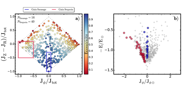
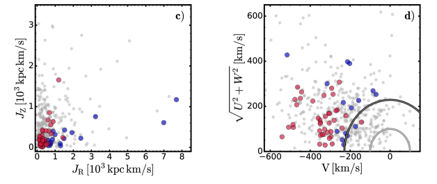
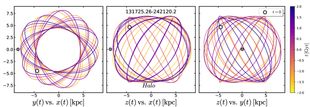
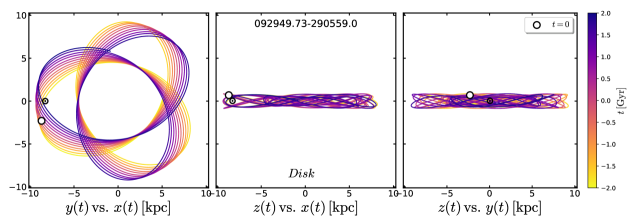
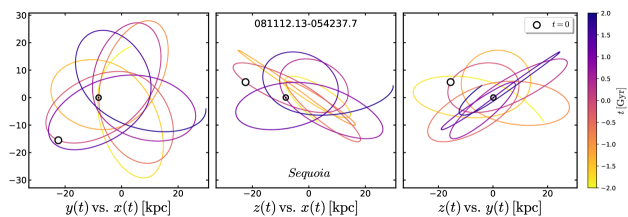
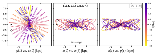
We find that out of the 475 analyzed stars, 16 stars are kinematically coincident with the Sausage accretion event, while 40 stars are candidate Sequoia members. As expected from their definition and the action map (Helmi et al., 2018; Belokurov et al., 2018; Myeong et al., 2019; Yuan et al., 2020), the latter are characterized by mildly eccentric $(e\sim 0.5)$ retrograde orbits, while the former have highly eccentric orbits $(e\sim 0.9)$. Appendix B shows some typical orbits for stars identified as possible Gaia Sequoia and Gaia Sausage members.

We remind the reader that our membership identification follows the criteria introduced in Myeong et al. (2019), and is thus entirely based on the dynamics through the use of the action map. We stress that this approach does not allow for any “background” population that may be present in these regions of the action map. Consequently, we cannot straightforwardly assume that all the stars in our sample that are dynamically coincident with the Sequoia/Sausage accretion events actually belong to such remnants. In Appendix A we have attempted to perform a more accurate analysis through the use of a clustering algorithm approach. Briefly, the clustering analysis of our very metal-poor sample does provide independent evidence for the existence of groupings consistent with the Sequoia (group 6) and Sausage (group 8) dynamical definitions, though there are also indications that our Sequoia and Sausage samples, as defined in Fig. 7, are potentially contaminated by a “background” population that might be as much as $\sim$ 50% and $\sim$35%, respectively. These background estimates are determined by exploiting the clustering analysis groupings discussed in Appendix A, and the numbers of stars within the Gaia Sequoia and Gaia Sausage loci.

Panels b), c), d) and e) of Figure 7 show a detailed analysis of stars identified as candidate Sequoia, shown in red, and Sausage members, shown in blue. In panel c) we note that, by construction, Sausage stars are characterized by more radial orbits, although at low $J_{\rm R}$, some candidate Sequoia stars seem to share the similar values of $J_{\rm R}$ as Sausage stars. The Toomre diagram in panel d) shows that both groups are consistent with halo dynamics, and again we note that there is some degree of overlap between the two groups of stars. As regards panel b), which shows the energy versus azimuthal action, Sausage candidates show the distinctive vertical distribution, indicative of almost null azimuthal angular momentum, while Sequoia stars are clearly highly retrograde, as expected. Comparing panel b) with Koppelman et al. (2019, their Figure 2) we note that our accreted candidates span a wider range in energy. However, we note that the definition of Sequoia and Sausage parameters differs from work to work. Indeed, Yuan et al. (2020) identifies Sausage members that lie well outside the selection box of Myeong et al. (2019) and the energy range of Koppelman et al. (2019). For the sake of our analysis, we choose to be consistent with the Myeong et al. (2019) classification, although we stress again that a number of the candidates may not actually belong to the remnants of the accretion events.

As regards abundances, we find that the most metal-poor star in our sample that is a candidate member of Sequoia (SMSS J081112.13-054237.7) has a metallicity of $\rm[Fe/H]=-3.74$, while the most metal-poor Sausage candidate (SMSS J172604.29-590656.1) has $\rm[Fe/H]=-3.31$ dex. Both stars come from the HiRes sample so that the abundance uncertainty is of order 0.1 (excluding any systematic uncertainties such as those arising from the neglect of 3D/NLTE effects). These values are quite consistent with the results of Monty et al. (2020). In that work, which uses dwarf stars, the lowest metallicity star plausibly associated with Sequoia, G082–023, has $\rm[Fe/H]=-3.59\pm 0.10$ while the most metal-poor star plausibly associated with Sausage, G064–012, has $\rm[Fe/H]=-3.55\pm 0.10$ (Monty et al., 2020).

Finally, for the stars in the HiRes, Jacobson+15 and Marino+19 samples, we are able to investigate the chemical patterns of the likely accreted stars. Panel f) of Figure 7 shows [$\rm\alpha$/Fe] vs. [Fe/H] for the 218 stars for which [$\rm\alpha$/Fe] values are available. Specifically, [$\rm\alpha$/Fe] is computed as the unweighted mean of [Mg/Fe], [Ca/Fe], [TiI/Fe] and [TiII/Fe] where available. The star SMSS J160540.18–144323.1 (Nordlander et al., 2019) has been arbitrarily plotted at a metallicity of [Fe/H]=–4.3 since otherwise it would be the only star with [Fe/H]<–5 in the panel. A visual inspection reveals that, with the single exception of SMSS J111201.72-221207.7, all the Sequoia and Sausage candidates are $\alpha$-enhanced, and no other trend is evident. Specifically, in our sample of very metal-poor Sequoia and Sausage candidates, we see no evidence for a “knee” in the ([$\rm\alpha$/Fe], [Fe/H]) relation. The metallicity of the knee marks the abundance where [$\rm\alpha$/Fe] begins to decrease with increasing [Fe/H] as the nucleosynthetic contributions from SNe Ia become increasingly important. Our result, however, is not inconsistent with the results of Matsuno et al. (2019) and Monty et al. (2020) who find evidence of the presence of a knee at higher abundances than any of the Sequoia and Sausage candidates plotted in Fig. 7. For example, Monty et al. (2020) indicate that the knee in Sequoia is at [Fe/H] $\approx$ –2 while that for Gaia Sausage is at [Fe/H] $\approx$ –1.6, values significantly more metal-rich than any of the candidates in Fig. 7.

5.2 A very metal-weak component in the Thick Disk?

It has recently been shown (Sestito et al., 2019, 2020b; Di Matteo et al., 2020; Venn et al., 2020) that, in contrast to the commonly accepted view, a significant fraction ($\sim 20\%$) of very low-metallicity stars resides in the MW disk rather than in the halo. Here we find a similar result: for the stars in our sample 102 out of 475 ($\sim 21\,\%$) exhibit disk-like dynamics in having orbits that are confined to within 3 kpc of the plane of the Milky Way.

The straightforward conclusion would be to propose these stars as supporting the existence of an extension to yet lower metallicities of the proposed Metal-Weak Thick-Disk (e.g., Chiba & Beers, 2000). However, a detailed analysis is required to discern the origin of these stars. Specifically, it is of key importance to understand if they are indeed disk-like stars, or if they are, for example, halo stars whose orbital plane happens to lie in the MW disk.

We therefore explore a number of orbital parameters to shed light on the nature of these stars. Specifically, Sales et al. (2009, and references therein) have shown how the orbital eccentricity can be used to probe the formation scenario of the Milky Way thick disk. Furthermore, as mentioned in the previous sections, the actions, and in particular the azimuthal action, provide important clues for the origin of a star. Here we couple these two orbital properties to disentangle the origin of the very low-metallicity stars residing in the MW disk.

As noted above, we classify as “disk” stars those with $|Z_{\rm max}|\leq 3\,\rm kpc$. This choice is made on the basis of the following considerations. First, Li & Zhao (2017) find that the (exponential) scale height of the MW thick disk is $z_{\rm 0}=0.9\pm 0.1\,\rm kpc$; it then follows that the vast majority of the thick disk population should be found within $\sim$3 scale heights, i.e., within $|Z_{\rm max}|$ = 3 kpc.

Second, Figure 8 shows the eccentricity distribution for different values of the maximum vertical excursion, from $2\,\rm kpc$ to $8\,\rm kpc$. For each panel, the yellow histogram (designated as “disk”) shows the distribution of stars within $N\,\rm kpc$, with $N=\{2,3,4,5,8\}$, while the grey shaded histogram (designated as “halo”) represents stars with $|Z_{\rm max}|>N\,\rm kpc$. As is evident from the figure, for heights above the plane exceeding 3 kpc, i.e., panels c), d) and e), the eccentricity distributions for the stars above and below the cut-off height become increasingly similar. On the other hand, for a cutoff value of $|Z_{\rm max}|=3\,\rm kpc$, an apparent difference is present in the sense the $e$-distribution for the low $|Z_{\rm max}|$ stars has a possible excess of intermediate eccentricity stars together with a possible narrow surfeit of stars with $e$ $\approx$ 0.85, which is also evident in panel a). However, application of both Kolmogorov-Smirnoff and Anderson-Darling tests (see, e.g. Scholz & Stephens, 1987) to compare the “disk” and “halo” distributions in panel b) revealed that the apparent differences are not statistically significant. Nonetheless, we adopt $|Z_{\rm max}|=3\,\rm kpc$ as the value of $|Z_{\rm max}|$ to discriminate between predominantly disk and predominantly halo populations. For completeness, we also note that if we choose $|Z_{\rm max}|$ cutoff values of 2.5 or 4 $\rm kpc$ and repeat the analysis discussed below, the outcomes are essentially unaltered.

Finally, the third reason for adopting a value of $|Z_{\rm max}|=3\,\rm kpc$ for the disk-like population is that it is consistent with Sestito et al. (2019, 2020b), allowing our results to be directly compared with theirs.

Figure 8: Eccentricity distribution of disk-like stars and halo-like stars for different choice of the cutoff $|Z_{\rm max}|$, from $2\,\rm kpc$, panel a), to $8\,\rm kpc$, panel e). In each panel, the eccentricity distribution for stars within $|Z_{\rm max}|\leq N\,\rm kpc$ is shown with the yellow histogram, while stars with $|Z_{\rm max}|>N\,\rm kpc$ are indicated by the grey shaded histogram. Stars with $D_{\rm apo}>$ 250 kpc are not considered. Panel b) also shows, as blue continuous curves, the outcome of applying Gaussian mixture modeling to the set of $e$-values for the disk-like stars, i.e., without any binning.

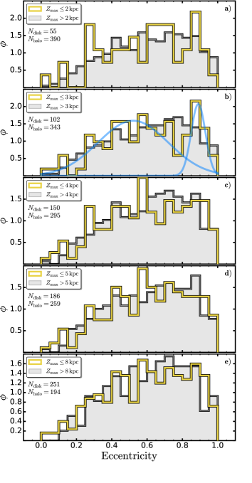
Looking again in detail at panel b) in Figure 8, we can see that the eccentricity distribution of the disk-like stars hints at the presence of two main groups. The first group has a relatively broad distribution peaking at $e\approx 0.55$ while the second population has a narrower distribution centred at $e\approx 0.85$. This interpretation is confirmed by the application of Gaussian Mixture Modeling to the $e$-distribution for the stars with $|Z_{\rm max}|\leq 3\,\rm kpc$, a process that does not require any choice as regards histogram bin size. The best-fit is for two Gaussians, one centred at $e=0.52$ containing 80% of the population and with a standard deviation of 0.14. The second Gaussian is centred at $e=0.89$ with a narrow $\sigma$ of 0.03. The two Gaussians are overplotted with blue thick lines in panel b) of Fig. 8. We shall refer to these two groups as the “low-eccentricity” and “high-eccentricity” populations, respectively, and adopt $e=0.75$ as the eccentricity to separate them.

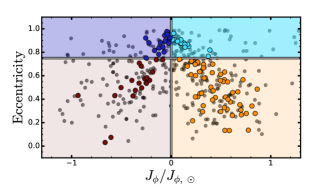
We now employ $J_{\rm\phi}$ to identify the motion of the disk stars as either prograde or retrograde. This is shown in Figure 9, where we mark retrograde high-$e$ and low-$e$ population stars with dark-blue and dark-red points, respectively, while prograde high-$e$ and low-$e$ group stars are indicated by azure and orange circles. Overall we find 72 low-$e$ stars (53 prograde and 19 retrograde) and 30 high-$e$ stars (15 prograde and 15 retrograde).

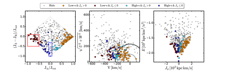
We then analyzed the orbital parameters of each of these sub-groups of disk-star candidates. The results are shown in Figure 10. The distributions shown in panels a) – j) are kernel density distributions computed by adopting a Gaussian kernel with a fixed value of 0.4 for the bandwidth scaling parameter, while the top three panels show the action map, the Toomre diagram, and the $E$ vs. $J_{\rm\phi}$ plot, respectively. The disk candidates are marked with different colours, as defined in Figure 9.

Figure 9: Eccentricity vs. azimuthal actions for all the stars in our sample (grey dots). Coloured filled points are for stars with $Z_{\rm max}\leq 3\,\rm kpc$. Specifically, stars on retrograde orbits with eccentricity greater and lower than $0.75$ are marked with dark-blue and dark-red circles, respectively. Prograde stars with eccentricity greater and lower than $0.75$ are indicated with azure and orange circles.

Figure 10: Top panels. Action map, Toomre diagram and energy vs. angular momentum for the stars with $|Z_{\rm max}|\leq 3\,\rm kpc$. The colours are the same as illustrated in Figure 9. Panels a) - h). Kernel density function of the orbital parameters of the identified four groups of disk stars.

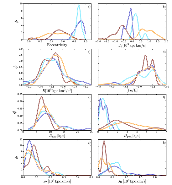
5.2.1 Low-eccentricity stars

In panel a) of Figure 10, it is interesting to see that the eccentricity distributions of the prograde and retrograde high-$e$ groups are almost identical, while, conversely, there are hints of a difference in the corresponding distributions for the low-$e$ stars. Specifically, the prograde low-$e$ stars (orange line) have a broader distribution while the retrograde low-$e$ stars (red line) have a narrower distribution peaking at $e\sim 0.5$-0.6. Together these $e$-distributions are quite consistent with the theoretical results in Sales et al. (2009), particularly as regards the $e$-distributions in the top-left panel of their Figure 3 (Sales et al., 2009). In that context the retrograde low-$e$ stars can be interpreted as an accreted population, while the prograde low-$e$ stars are likely “in-situ”, i.e., born within the thick-disk of the Galaxy.

To support this interpretation we consider again the action map, here shown in the upper-left of Figure 10 with the $|Z_{\rm max}|\leq 3\,\rm kpc$ stars identified. It is evident from this panel that the majority of the retrograde low-$e$ stars fall within the locus defining the Gaia Sequoia accretion event, consistent with these stars having an accretion origin. Comparing the corresponding panels in Figures 7 and 10 for the Toomre diagram and the Energy $(E)$ against azimuthal action $(J_{\rm\phi})$ diagram, respectively, confirms the connection.

Regarding the prograde low-$e$ stars, a substantial number of these fall in the region of the Toomre diagram usually restricted to disk stars; their rotation velocities lag that of the Sun by relatively small amounts, less than 100 $\rm km\,s^{-1}$ in some cases. We therefore conclude that the prograde low-$e$ stars define a very metal-weak component to the Galaxy’s thick disk. This conclusion is supported by the eccentricity distribution of the stars, which agrees well with the eccentricity distributions for (more metal-rich) thick-disk stars shown in Li & Zhao (2017, their Figure 12 and 14).

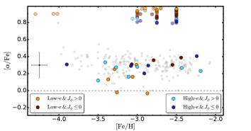
These 53 low-$e$, low $Z_{\rm max}$ prograde stars represent $\sim$ 11% of our total sample. Of these 53, 6 are included in the high-dispersion data sets and the [$\alpha$/Fe] versus [Fe/H] for these stars is shown in Figure 11. Four of the 19 low-$e$, low $Z_{\rm max}$ retrograde stars are also included on the plot along with the remainder of the stars in the high-dispersion data sets. For completeness as regards the [Fe/H] distributions of the samples, we also show in the upper part of the figure the [Fe/H] values for the remainder of the prograde and retrograde low-$e$, low $Z_{\rm max}$ samples. Detailed abundance information, such as [$\alpha$/Fe], is not available for these stars that arise from the LowRes sample. Further, in order to avoid any potential systematic effects, we have chosen not to plot the [$\alpha$/Fe] values for the 3 low-$e$, low $Z_{\rm max}$ Sestito+19 sample stars in Figure 11. The stars are BD+44 493 ([Fe/H] = –4.30), 2MASS J18082002-5104378 ([Fe/H] = –4.07) and LAMOST J125346.09+075343.1 ([Fe/H] = –4.02) and all 3 have prograde orbits. The [Fe/H] values for these stars are taken from Table 1 of Sestito et al. (2019).

It is evident from the figure that, though the sample is very limited, the four retrograde low-e stars show no obvious difference in location in this plane from the remainder of the (halo dominated) sample with high-dispersion abundance analyses. The location of the six prograde low-e stars, however, is intriguing despite the small numbers. It appears that the mean [$\alpha$/Fe] for these stars is lower than that for the full sample by perhaps 0.15, and two of the stars, namely SMSS J230525.31-213807.0 which has [Fe/H] = –3.26 and which is also known as HE 2302-2154a, and SMSS J232121.57-160505.4 ([Fe/H] = –2.87, HE 2318-1621), are among the small number (of order a dozen in total) that have [$\alpha$/Fe] $<$ 0.1 in the high-dispersion samples. Such $\alpha$-poor stars, also referred to as “Fe-enhanced” stars (e.g. Yong et al., 2013; Jacobson et al., 2015), may reflect formation from gas enriched in SNe Ia nucleosynthetic products that, if valid, may have implications for the epoch at which these stars settled into, or formed in, the thick disk (see also Sestito et al., 2019, 2020b; Di Matteo et al., 2020). However, we consider further discussion of the element abundance distributions in these stars beyond the scope of the present paper.

The overall [Fe/H] distribution of the retrograde and prograde stars as inferred from Figure 11 is similar to that for the full sample. The star with the lowest combination of metallicity and eccentricity in our sample of prograde, low $Z_{\rm max}$ stars is SMSS J190836.24–401623.5 that has [Fe/H] = –3.29 $\pm$ 0.10 and for which we find $e$ = 0.29 and a high $V$ velocity of –21 km s^-1. We also note that the orbital parameters derived here for the UMP star 2MASS J1808002–5104378, which is included in our Sestito+19 data set, are very similar to those found in Sestito et al. (2019). Specifically we find for this star $e$ = 0.13 and $V$ = –29 km s^-1, while Sestito et al. (2019) list values of 0.09 and –45 km s^-1, respectively. Moreover, as noted by Sestito et al. (2019), the “Caffau-star” (Caffau et al., 2011), which is an apparently carbon normal (i.e., [C/Fe] $<$ 0.7) dwarf (and therefore not included in our sample) with [Fe/H] $\approx$ –5.0, and which is the star with the lowest total metal abundance known to date, is a further example of an ultra-low metallicity star with a disk-like orbit. Sestito et al. (2019) determine that this star has a prograde orbit with $e$ = 0.12 that is confined to the Galactic plane, and which has a high $V$ velocity of –24 km s^-1. We agree with the suggestion of Sestito et al. (2019) that these stars may have formed in a gas-rich “building-blocks” of the proto-MW disk. The origin of these stars is also discussed within the context of the theoretical simulations presented in Sestito et al. (2020a). The simulations reveal the ubiquitous presence of populations of low-metallicity stars confined to the disk-plane. In particular, the simulations show that the prograde planar population is accreted during the assembly phase of the disk, consistent with our interpretation and that of Sestito et al. (2019).

Panels b)-h) of Figure 10 show the kernel density distributions of the other orbital parameters. These distributions do not exhibit clear differences between prograde and retrograde low-$e$ stars, with the possible exception of $D_{\rm apo}$, in panel e), and $D_{\rm peri}$, in panel f), which mimic the differences in the eccentricity distribution evident in panel a).

We conclude that the low $Z_{\rm max}$ prograde and retrograde low-$e$ stars likely have different origins, with the former possibly being formed in-situ in the Galaxy’s thick disk while the latter are likely accreted from disrupted Milky Way satellites. Whether these latter stars belong to the Sequoia main remnant, or its higher-energy tails (Thamnos 1 and 2, Koppelman et al., 2019) is beyond the scope of the present work, although, as panel a) of Figure 10 shows, most fall within the region defining Sequoia stars.

Figure 11: [$\alpha$/Fe] vs. [Fe/H] for the stars in the HiRes, Jacobson+15 and Marino+19 samples. Low-$e$, low-$Z_{\rm max}$ prograde and retrograde stars are marked with orange and dark-red points, respectively, while high-$e$, low-$Z_{\rm max}$ prograde and retrograde stars are shown with azure and dark-blue colours. Stars from the LowRes sample, for which only [Fe/H] values are available, are arbitrarily placed between [$\alpha$/Fe]=0.79 and [$\alpha$/Fe]=0.95 on the y-axis. This is to allow an assessment of the [Fe/H] distributions of the samples. The (non-physical) range of [$\alpha$/Fe] values is needed to separate the points as the [Fe/H] values in the LowRes sample are generally quantized at 0.25 dex values. This also applies to the 3 orange points with [Fe/H] $\leq$ –4.0 that are from the Sestito+19 dataset. For the stars with high dispersion spectroscopic abundances, the typical uncertainty in [Fe/H] is $\pm$0.1 dex and $\pm$0.15 dex in [$\alpha$/Fe], as indicated by the black point on the left side. For the stars from the LowRes sample the typical uncertainty in [Fe/H] is $\pm$0.3 dex. The dashed line indicates [$\alpha$/Fe] = 0.

5.2.2 High-eccentricity stars

The interpretation of the 30 low $Z_{\rm max}$, high-$e$ stars in our sample is less straightforward, since, as the panels of Figure 10 reveal, nearly all their orbital parameters show similar distributions for the prograde and retrograde stars, with the only exception being the azimuthal action (by construction). We note first that the only mechanism able to explain, at least qualitatively, the occurrence of disk stars with high-eccentricity orbits, is the heating mechanism discussed in Sales et al. (2009, e.g., Figure 3). Some of the stars in this sub-sample could therefore be disk stars heated by accretion events. Alternatively, some could simply be halo stars that happen to have orbital planes that lie close to the Milky Way disk plane.

However, even though these high-$e$ stars do not satisfy the Gaia Sausage Myeong et al. (2019) membership criteria, we find that many qualitatively share its typical orbital properties: high-eccentricity, low or no angular momentum, small Galactic pericenters, Galactic apocenters as great as $\sim 20$-$25\,\rm kpc$ and strong radial motions. We therefore argue that at least some stars could be associated with the Sausage accretion event. In support of this conjecture, we note that they are consistent with the Yuan et al. (2020) classification for Gaia Sausage stars, both in the action map locus, and in the energy regime.

Myeong et al. (2019) suggest that the Sausage accretion event was an almost head-on collision with the Milky Way. Such an event generates orbits with small perigalacticons that are strongly radial, eccentric, and with roughly equal numbers of prograde and retrograde stars. These are the properties that we see for our low $Z_{\rm max}$, high-$e$ stars and it therefore seems reasonable to conclude that many of our low $Z_{\rm max}$, high-$e$ stars have their origin in the Sausage accretion event.

For seven of the 15 prograde high-$e$, low $Z_{\rm max}$ stars, detailed abundances are available from our high-dispersion data sets. The [$\alpha$/Fe] abundance ratios are shown as a function of [Fe/H] in Figure 11. The corresponding data for 5 of the 15 retrograde stars are also shown in the figure. The [Fe/H] values for the remainder of the stars in these groups are shown across the top of the plot. The numbers of stars with high-dispersion analyses in both high-$e$, low $Z_{\rm max}$ sub-samples are small, but there does not appear to be any obvious difference between them and the distribution of the full sample.

5.3 The candidate unbound stars

Figure 12: Panel a). Barplot of the percentage of unbound realizations for the 35 stars with apparent $D_{\rm apo}\geq 250\,{\rm kpc}$. The names of the stars are listed in the panel below panels c) and d). Each bar is colour-coded according to the percentage of $N_{\rm unbound}$, as shown in the top colour bar. Panel b). Energy against apparent apogalacticon distance. Filled circles indicate stars with negative energy, while filled squares mark those with positive energy. The black vertical dashed line marks the Milky Way tidal radius (250  kpc), while the stars with $D_{\rm apo}<250\,\rm kpc$ are shown as grey shaded points. Panel c) and Panel d) show the Energy against the perigalacticon distance $(D_{\rm peri})$ and the Energy against the azimuthal action $(J_{\rm\phi})$. Individual error bars are shown in panels b), c) and d). Panel e). [$\alpha$/Fe] vs. [Fe/H] for the candidate unbound stars that occur in the HiRes, Jacobson+15 and Marino+19 samples. As in Fig. 7, the star SMSS J160540.18–144323.2 (Nordlander et al., 2019) is shown with a star-like symbol placed at [Fe/H]=–4.3. As for the other panels, filled circles indicate stars with negative energy, while filled squares mark those with positive energy. The remainder of the stars in our high-dispersion samples are shown as light-grey circles. The metallicity estimates for the 4 stars not in our high dispersion samples are plotted at the top of the panel.

As introduced in Section 4, we find 30 stars with potentially unbound orbits, defined by having an apparent $D_{\rm apo}\geq 250\,{\rm kpc}$. One star, HE 0020–1741, comes from our subset of the Sestito+19 sample. Sestito et al. (2019) list $D_{\rm apo}\approx 296\,\rm kpc$ for this star, the largest value in their determinations, while in the Mackereth & Bovy (2018) catalogue the star is classified as unbound in accord with our result. The remaining 29 stars are from the SkyMapper samples.

To test the sensitivity of the results to the adopted potential we investigated the orbits of these stars using a different choice of the potential, namely the GALPY MWPotential2014. The calculations reveal that all 30 stars again have $D_{\rm apo}>250\,\rm kpc$. In addition, for this choice of potential, we find that the star SMSS J044419.01–111851.2 may also be unbound; it is on a loosely bound orbit in the McMillan2017 potential with an apogalacticon distance of $\sim 200\,\rm kpc$.

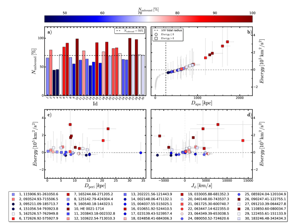
In order to shed light on the nature of these stars we have investigated the distributions of the 500 random realizations of the orbits, together with the corresponding orbital parameters, such as the apparent apo/peri-galacticon distance ratio $(D_{\rm apo}/D_{\rm peri})$, the energy ($E$) and the azimuthal action $(J_{\rm\phi})$. Panels a) – d) of Figure 12 show the information for the 30 potentially unbound stars.

Since the direct orbit integration for the observed positions and velocities resulted in unbound orbits (apparent $D_{\rm apo}>250\,\rm kpc$), it would be incorrect to adopt the uncertainties as defined in Section 3.2 for all parameters. Specifically, for these stars we opt not to give uncertainties for the apparent $D_{\rm apo},\,e,\,Z_{\rm max}$ and $J_{\rm R}$ values since the medians for the 500 realizations and the “observed” values, i.e., the values from the observed properties, differ significantly. On the other hand, for the remaining orbital parameters, namely $D_{\rm peri},\,E,\,J_{\rm\phi},\,J_{\rm Z},$ and the $U,\,V,\,W$ velocities, the median values are consistent with the observed ones, and therefore we compute the uncertainties in these quantities as before, from the difference between the $16^{\rm th}$ and the $84^{\rm th}$ percentile of the PDFs.

Panel a) of Figure 12 shows the fraction of unbound realizations for each star. Each bar is colour-coded according to its percentage, from a minimum of 42.6% for SMSS J095211.09–185713.7 (number 3 in the identification panel in the Figure 12) to a maximum of 100% for SMSS J090247.41–122755.1 (#26). White- and reddish colour tones indicate stars with a fraction of unbound orbits greater than 70%, which we take as a conservative value to identify likely unbound stars. Blueish colours represent stars with a lower unbound fraction. A visual inspection of panel b) reveals that nearly all stars with $N_{\rm unbound}>70\%$ exhibit positive energies, thus confirming that they are likely to be escaping from the Galaxy. Overall, we find that 17 stars have $N_{\rm unbound}>70\%$, and of these 15 have $E>0$ (the two stars with $N_{\rm unbound}>70\%$ but $E\leq 0$ are numbers 22 and 23). Panel b) also shows that four stars (numbers 1, 8, 11, 13) have a positive energy, but with $N_{\rm unbound}$ slightly below 70%. We consider these stars as also likely unbound, bringing the total number of candidate unbound stars to 21, or 4.4% of the total sample. We note in particular that aside from HE 0020–1741 (#10), three further stars in our set of 21 unbound candidates are also classified as unbound in the Mackereth & Bovy (2018) catalogue. These are the bright $r$-process element enhanced star SMSS J203843.18–002332.8 (#11, RAVE J203843.2–002333, Placco et al., 2017), together with SMSS J183246.48–343434.3 (#30) and SMSS J202221.56–121443.9 (#13). On the other hand, one of our stars, SMSS J103622.54-713010.3 (#12), has a bound orbit in the Mackereth & Bovy (2018) catalogue. There are no stars in common with the list of 20 ‘clean’ high-velocity star candidates with unbound probability exceeding 70% in Marchetti et al. (2019).

The remaining nine stars have negative (bound) energies, although the values are consistent with zero within their uncertainties. Their classification is thus uncertain as they could be unbound or on loosely bound orbits. None are found in the Mackereth & Bovy (2018) catalogue.

We now speculate as to the origin of these stars, proposing three possible physical mechanisms that could provide each star with sufficient energy to escape the Galaxy.

• A star in a close binary can be expelled from the Galactic Centre via an interaction with the central black hole. The clearest example of this process is the star S5-HVS1 discussed in Koposov et al. (2020).

• A star can acquire high velocity (of order of the binary’s pre-SNe explosion orbital velocity) from being in a binary when the companion explodes as a supernova (e.g., Eldridge et al., 2011).

• A star can acquire energy as part of a gravitational interaction involving the merger of a dwarf galaxy with the Milky Way (e.g., Abadi et al., 2009).

For the first mechanism to happen, the star has to have an origin close to the Galactic Centre, which means that its $D_{\rm peri}$ should be near zero. However, as panel c) of Figure 12 shows, only one star (SMSS J115906.91–261050.6, #1, $D_{\rm peri}$ = 0.26 kpc) has a perigalacticon distance within 1 kpc of the Galactic Centre, while the remainder of the candidates have $D_{\rm peri}>1\,{\rm kpc}$. This suggests that the first possibility is unlikely, particularly when it is recognised that all the stars in the sample are giants and therefore unlikely to be in a sufficiently compact binary.

The second mechanism also seems unlikely because the unbound stars are all giants with, as a consequence, relatively large stellar radii. As a result, the separation between the components of any pre-SNe binary containing the star is unlikely to be sufficiently small that the orbital velocity, which underlies the “kick velocity” provided when the companion becomes a SNe, would be sufficiently high that the liberated star is no longer bound to the Galaxy. Furthermore, at least for those stars where high dispersion spectra are available, there is no evidence of any “pollution” from the SNe event.

This leaves us with the third possible origin, which is plausible given that it is generally accepted that the formation of the Galactic halo is driven by the accretion and tidal disruption of dwarf galaxies (e.g., the recent discovery of remnants of accretion events: Helmi et al., 2018; Belokurov et al., 2018; Koppelman et al., 2019; Myeong et al., 2019). Specifically, we postulate that our set of unbound stars originated in the outskirts of dwarf galaxies that were accreted by the Milky Way, gaining energy from the gravitational interaction that resulted in the disruption of the dwarfs. Given the relatively low metallicities of the unbound stars, which range from –4 (or less) to –2 in [Fe/H] (see the lowermost panel of Fig. 12), we speculate that the disrupted systems were relatively low-mass, low-metallicity systems.In this context, we note that 16 out of 21 stars have prograde orbits, while 5 have negative $J_{\rm\phi}$ and thus a retrograde orbit. This likely indicates that multiple accretion events may be involved. However, it is necessary to keep in mind that the timescale for an unbound star to reach the virial radius from the inner regions of the Galaxy is $\sim$ 1 Gyr. Consequently, the gravitational interactions that generated the unbound stars in our sample likely occurred relatively recently, which may argue against the proposed “origin in accretion events” scenario. Detailed evaluation of the orbits of the unbound stars, individually and collectively, is required to assess the situation and to investigate their origins(s). The metallicities of other candidate unbound stars, such as those in Marchetti et al. (2019) will also provide important input (e.g., Hawkins & Wyse, 2018).

We note also that there is a fourth possibility, that uncertainties in the analysis lead to incorrect orbital parameters. For example, if the distance to the star used in calculating the orbit were overestimated, this could result in unbound or nearly-bound status. This is the likely explanation for the discrepancy concerning the star SMSS J103622.54–713010.3 (unbound here, bound in the Mackereth & Bovy (2018) catalogue) as our adopted distance is more than a factor of two larger than the Bailer-Jones et al. (2018) distance. The availability of improved parallaxes and stellar parameters from the forthcoming Gaia EDR3 and DR3 releases will help alleviate these discrepancies. As another possibility, we note that the total mass of the Galaxy may in fact be larger than that used in our modeling. If this is the case then, although on high-energy orbits, the stars would remain bound (e.g., Monari et al., 2018; Fritz et al., 2020).

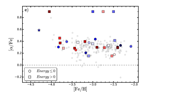
Panel e) of Figure 12 shows the [$\alpha$/Fe] vs. [Fe/H] relation for 26 of the 30 candidate unbound stars that are in our high-dispersion samples, together with the values for the remainder of the stars from the high dispersion samples. The estimates of [Fe/H] for the remaining 4 stars, from the LowRes data set, are shown at the top of the panel. It is evident from this panel that candidate unbound stars are not distinguished from the full sample as regards the overall metallicity distribution or the [$\alpha$/Fe] distribution.

6 Summary and conclusions

In this work we have analyzed a sample of 475 very metal-poor giant stars, most of which have originated from the SkyMapper search for the most metal-poor stars in our Galaxy (Da Costa et al., 2019). The data set covers a metallicity range of almost five dex $(-6.5<{\rm[Fe/H]}\leq-2)$, and together with the relatively large number of stars, makes it ideal to investigate the kinematics, and ultimately the origin, of these very rare and important objects together with the implications for the formation of the Milky Way.

We first exploited the action map for our sample together with the classification criteria of Myeong et al. (2019) to identify candidate members of the Gaia Sausage and Gaia Sequoia accretion events. We find 16 stars dynamically consistent with Gaia Sausage and 40 with Gaia Sequoia. While we cannot be certain all candidates are in fact associated with these entities, the lowest metallicities ([Fe/H] = –3.31 for Gaia Sausage and –3.74 for Gaia Sequoia) are quite consistent with the findings of Monty et al. (2020). With a single exception, all our candidate Gaia Sausage and Gaia Sequoia stars for which we have high-dispersion spectra are $\alpha$-rich, similar to the general halo population. This is again consistent with the results of Monty et al. (2020).

The recent work of Sestito et al. (2019, 2020b), Di Matteo et al. (2020) and Venn et al. (2020) has revealed an unexpected significant population of very low-metallicity stars residing in the plane of the Galaxy. We find a similar result in that $\sim 21\,\%$ of the stars in our sample have orbits that remain confined to within 3 $\rm kpc$ of the Galactic plane. Moreover, these stars show a different eccentricity distribution compared to the stars with larger $|Z_{\rm max}|$ values, pointing towards a different origin and/or evolution compared to the (halo dominated) bulk of the sample.

Our detailed analysis of these low $|Z_{\rm max}|$ stars reveals four sub-populations as regards orbit eccentricity and prograde or retrograde motion. Of particular interest are the stars with relatively low eccentricities ($e<0.75,{\rm median}\approx 0.5)$ and prograde velocities. These stars, which make up $\sim$ 11% of the total sample, have metallicities at least as low as [Fe/H] = –4.3 and are best interpreted as revealing the existence of a very low-metallicity tail to the Galaxy’s metal-weak thick disk population (e.g. Chiba & Beers, 2000). On the other hand, the low-$e$ retrograde stars that have $|Z_{\rm max}|\leq 3\,\rm kpc$ ($\sim$ 4% of the sample) are most likely an accreted population. We also find a population ($\sim$ 6% of the sample) of low $|Z_{\rm max}|$ stars that have high eccentricity orbits (${\rm median}\approx 0.88$) with small pericenters and which are split equally between prograde and retrograde motion. It seems likely that many of these stars might be associated with the Gaia Sausage accretion event (Myeong et al., 2019; Yuan et al., 2020; Koppelman et al., 2019). With the possible exception of the low-$e$, low $|Z_{\rm max}|$ prograde stars that may have a somewhat lower mean [$\alpha$/Fe] abundance ratio, none of the four sub-populations with low $|Z_{\rm max}|$ are distinguished, as regards [$\alpha$/Fe] or [Fe/H], from the full set of stars for which high-dispersion based analyses are available.

Finally, we find that a small fraction of our sample (21 stars, $\sim$ 4.4%) are likely to be escaping from the Galaxy, i.e., are on orbits that are not bound. The [Fe/H] and [$\alpha$/Fe] distributions of these stars are not distinguished from those for the full sample; for example, their metallicities are spread from –4 (or less) to –2 in [Fe/H]. Our preferred interpretation for these stars is that they have acquired sufficient energy to escape from the Galaxy via the gravitational interaction that occurs when infalling dwarf galaxies are tidally disrupted by the Milky Way.

Data availability

The data underlying this article are available in the article and in its online supplementary material.

Appendix A Clustering analysis

As an alternative approach, we analyzed our sample of stars exploiting the scikit-learn Spectral clustering algorithm (Pedregosa et al., 2011). This analysis has the advantage of being almost completely independent from our choices (i.e., limiting $|Z_{\rm max}|$, prograde/retrogade etc.), while on the other hand has the limitations of being a “blind” analysis. Specifically, in order for the result to be trustworthy, we should have knowledge of how the selection biases (e.g., bright stars in the solar neighbourhood, uncrowded stellar environments and the other effects discussed in Da Costa et al. (2019)) propagate into the cluster choices. Unfortunately, it is not possible to quantify these biases.

Nonetheless, we believe that it is worth exploring this fully independent classification approach. The clustering has been performed in the 4-dimensional space with the three actions and the eccentricity ($J_{\rm R},\,J_{\rm\phi},\,J_{\rm Z},\,e$) with the following input parameters: affinity$=$nearest_neighbors and assign_labels$=$discretize.

Figure 13: Top row. Same as the top row Figure 10 except stars are colour-coded by group. The group colours are identified at the top of the panels. Panels a1)-e2). Kernel density distributions of the computed orbital parameters for the groups identified by the clustering algorithm. In the panels with suffix 1 we represent the distributions for groups 2 to 4, while panels with suffix 2 show groups 5-8. The kernel density estimates of the orbital parameters for group 1 (G1) are not shown for scaling reasons.

Figure 14: Panels f1)-j2). Same as panels a1)-e2) of Figure 13.

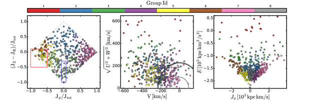
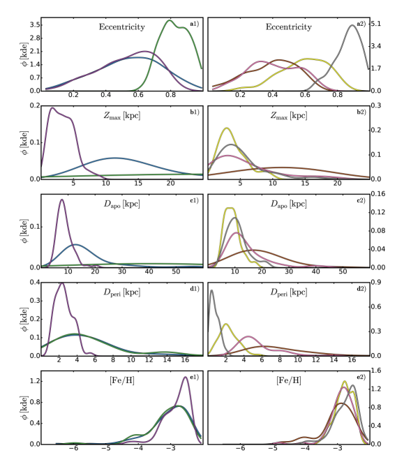
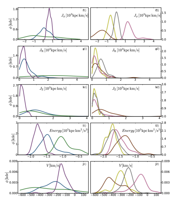
Figure 13 shows the results of the clustering analysis. In the top three panels we show the same top three panels as for Figure 10 but now for the 8 identified clusters. We note that group # 1 (red markers with coordinates $(0,-1)$ in the action map) is the group of unbound stars, and therefore is not investigated further in the lower panels. Panels a1)–e2) in Figure 13 and panels f1) to j2) in Figure 14 then show the kernel density distributions of different orbital parameters for each sub-group, with groups 2–4 in the left panels and groups 5–8 in the right panels. A comparison of Figures 13 and 14 with Figure 10 suggests the following.

• group # 1 (G1, red markers, 28 stars) is composed of stars with energies consistent or greater than 0, visible in the top-right panel of Figure 13. These stars have apparent apogalacticon distances larger than the Milky Way virial radius, i.e., 250 kpc. They are characterized by large values of the radial action, $J_{\rm R}$, which translates in $J_{\rm\phi}/J_{\rm tot}\sim 0$ and $(J_{\rm Z}-J_{\rm R})/J_{\rm tot}\sim-1$. Overall, we find that 28 stars are grouped in G1. All of these stars are in the sub-sample discussed in Section 5.3, although two stars in the Section 5.3 sub-sample, namely SMSS J095211.09–185713.7 and SMSS J002148.06–471132.1, are not classified as G1 stars, despite having apparent $D_{\rm apo}$ larger than 250 kpc. These two stars have negative (bound) energies and are classified by the clustering algorithm in Group #7 (pink points), which is composed of stars on loosely bound orbits. There is therefore essentially no discrepancy between the sub-sample discussed in Section 5.3 and the high-energy G1 stars identified by the clustering algorithm. We do not show the kernel density distributions of these stars in the subsequent panels for scaling reasons.

• group # 2 (G2, blue markers, 93 stars) are a combination of prograde and retrograde halo stars. We note that they span quite a wide energy range, but we find difficult to draw further conclusions. Presumably this group is made up of a mixture of in-situ and accreted halo stars.

• group # 3 (G3, green markers, 54 stars) is a mixture of prograde and retrograde stars on loosely bound orbits, that venture far from the Galactic plane.

• group # 4 (G4, purple markers, 61 stars) partially overlaps with low-$e$ stars in all three of the top-panels of Figure 10. Furthermore, their eccentricity distribution peaks at $e\sim 0.4-0.6$, while most of them remain roughly confined within $5\,\rm kpc$ of the Galactic plane and 20 kpc from the Galactic centre. A possible interpretation would be to consider these stars as thick-disk stars. This hypothesis is also supported by the Toomre diagram in the top center panel of of Figure 13, where purple stars occupy a locus typical of thick-disk stars. By the comparison with Figure 10 we find a partial match of this group with the low-$e$ prograde population (orange points), identified as candidate very metal-weak thick disk stars.

• group # 5 (G5, yellow markers, 53 stars) partially shares the location of the low-$e$ and retrograde population (red dots in Figure 10) as well as partially overlapping with the locus of the Sequoia remnants identified in Myeong et al. (2019). The eccentricity distribution peaks at about $e\sim 0.6$, and they are confined to the inner halo ($D_{\rm apo}\leq 10\,\rm kpc$). Panel b1) of Figure 13 shows that $\sim 80\%$ of these stars are confined within $5\rm\,kpc$ from the Galactic plane. Most of them don’t orbit further than 10 kpc from the Galactic centre. Comparing then the top-right panels of Figure 13 with Koppelman et al. (2019, bottom-right panel of their Figure 2), we see that G5 stars have a higher energy (in absolute values) than Gaia Sequoia stars, while their energy and their angular momentum suggest a possible association with the Thamnos 1/2 groups (Koppelman et al., 2019).

• group # 6 (G6, brown markers, 37 stars) is composed of stars with very retrograde and mildly-eccentric orbits that venture far from the Galactic plane and from the Galactic centre, with $Z_{\rm max}$ and $D_{\rm apo}$ peaking at $\sim$15-20 kpc. These stars have energies that range from $\sim-1$ to $\sim-1.7\;[10^{5}\,\rm kpc\cdot km^{2}\,s^{-2}]$. This group is consistent with the identification of the Gaia Sequoia remnants in Koppelman et al. (2019).

• group # 7 (G7, pink markers, 67 stars) partially overlaps with G4 both in the action map and in the Toomre diagram, while it is well-defined in the Energy vs. $J_{\rm\phi}$-plane. Panel a2) of Figure 13 shows that the eccentrity distribution of these stars is double peaked, with the first peak at $e\sim 0.3$ and a second one at $e\sim 0.6$. Given the distribution of $D_{\rm apo}$ and $Z_{\rm max}$ it would seem that these stars are a mixture of halo and thick-disk stars, with lower binding energies than their G4 counterparts. As for G4, we note that there is a clear overlap between this group and the low-$e$ prograde stars shown in Figure 10.

• group # 8 (G8, grey markers, 82 stars) share roughly the same location of the high-$e$ both retrograde and prograde population (azure and navy dots in Figure 10) in all top three panels of Figure 13. Furthermore, the distribution of their orbital parameters nearly overlaps with those of the combined high-$e$ prograde and retrograde populations. Their energy and angular momentum agrees with the Gaia Sausage definition in Yuan et al. (2020). We find particularly interesting the pericenter/apocenter distributions, whose analysis suggest that most of these stars move back and forth from the Galactic centre to the Galactic outskirts, always remaining within few $\rm kpc$ from the Galactic plane ($\sim$60% these stars are indeed confined within $5\,\rm kpc$ from the plane). Given the observed orbital properties, and in particular the perigalacticon distances as low as $\sim$1 kpc, we speculate that such a remnant can be formed via a “head-on” accretion event, as in the Sausage progenitor (Myeong et al., 2019).

It is clear that the two different analyses (discussed here and in Section 5) reach qualitatively the same conclusions. First, we find solid evidence for the existence of a very metal-weak component in the Galactic thick disk. Further, from the analysis of the orbital actions and by means of the action map, we have identified possible members of the Gaia Sequoia and Gaia Sausage accretion events. The analysis also suggests that the low $|Z_{max}|$, high-$e$ population that is composed of stars with both prograde and retrograde orbits, may also be associated with the Gaia Sausage event. Both analyses also identify a consistent set of candidates that are likely not bound to the Galaxy.

Appendix B Example orbits

In the following we show four typical orbits of Halo, very metal-weak thick disk, Sequoia and Sausage stars within our sample. Each orbit is colour coded according to the integration time, while the white dot represents the current position in the Galactocentric cartesian reference frame. As discussed in Section 3.2, each orbit has been integrated in a McMillan2017 potential (McMillan, 2017) backward and forward in time for 2$\,\rm Gyr$. The actions have been computed with the Stäckel fudge method implemented in GALPY.

Figure 15: From top to bottom: typical orbit in the Galactocentric cartesian frame for examples of Halo, very metal-weak thick disk, Sausage and Sequoia stars, respectively. Each orbit is colour coded according to the integration time, and the white point indicates the current position of the star. The position of the Sun is indicated by the circled dot. Note that the orbit for the Sequoia star shown in the third row is much larger than for the other three stars.

References

- Abadi et al. (2009) Abadi M. G., Navarro J. F., Steinmetz M., 2009, ApJ, 691, L63
- Aguado et al. (2019) Aguado D. S., et al., 2019, MNRAS, 490, 2241
- Bailer-Jones et al. (2018) Bailer-Jones C. A. L., Rybizki J., Fouesneau M., Mantelet G., Andrae R., 2018, AJ, 156, 58
- Beers & Christlieb (2005) Beers T. C., Christlieb N., 2005, ARA&A, 43, 531
- Beers et al. (1992) Beers T. C., Preston G. W., Shectman S. A., 1992, AJ, 103, 1987
- Beers et al. (2014) Beers T. C., Norris J. E., Placco V. M., Lee Y. S., Rossi S., Carollo D., Masseron T., 2014, ApJ, 794, 58
- Belokurov et al. (2018) Belokurov V., Erkal D., Evans N. W., Koposov S. E., Deason A. J., 2018, MNRAS, 478, 611
- Bernstein et al. (2003) Bernstein R., Shectman S. A., Gunnels S. M., Mochnacki S., Athey A. E., 2003, in Iye M., Moorwood A. F. M., eds, Society of Photo-Optical Instrumentation Engineers (SPIE) Conference Series Vol. 4841, Instrument Design and Performance for Optical/Infrared Ground-based Telescopes. pp 1694–1704, doi:10.1117/12.461502
- Bessell et al. (2015) Bessell M. S., et al., 2015, ApJ, 806, L16
- Binney (2012) Binney J., 2012, MNRAS, 426, 1328
- Binney & Spergel (1984) Binney J., Spergel D., 1984, MNRAS, 206, 159
- Bland-Hawthorn & Gerhard (2016) Bland-Hawthorn J., Gerhard O., 2016, ARA&A, 54, 529
- Bovy (2015) Bovy J., 2015, ApJS, 216, 29
- Brook et al. (2007) Brook C. B., Kawata D., Scannapieco E., Martel H., Gibson B. K., 2007, ApJ, 661, 10
- Caffau et al. (2011) Caffau E., et al., 2011, Nature, 477, 67
- Cayrel et al. (2004) Cayrel R., et al., 2004, A&A, 416, 1117
- Chiba & Beers (2000) Chiba M., Beers T. C., 2000, AJ, 119, 2843
- Christlieb et al. (2008) Christlieb N., Schörck T., Frebel A., Beers T. C., Wisotzki L., Reimers D., 2008, A&A, 484, 721
- Cui et al. (2012) Cui X.-Q., et al., 2012, Research in Astronomy and Astrophysics, 12, 1197
- Da Costa et al. (2019) Da Costa G. S., et al., 2019, MNRAS, 489, 5900
- Demarque et al. (2004) Demarque P., Woo J.-H., Kim Y.-C., Yi S. K., 2004, ApJS, 155, 667
- Di Matteo et al. (2020) Di Matteo P., Spite M., Haywood M., Bonifacio P., Gómez A., Spite F., Caffau E., 2020, A&A, 636, A115
- Eggen et al. (1962) Eggen O. J., Lynden-Bell D., Sandage A. R., 1962, ApJ, 136, 748
- El-Badry et al. (2018) El-Badry K., et al., 2018, MNRAS, 480, 652
- Eldridge et al. (2011) Eldridge J. J., Langer N., Tout C. A., 2011, MNRAS, 414, 3501
- Frebel & Norris (2015) Frebel A., Norris J. E., 2015, ARA&A, 53, 631
- Fritz et al. (2020) Fritz T. K., Di Cintio A., Battaglia G., Brook C., Taibi S., 2020, MNRAS, 494, 5178
- Gaia Collaboration et al. (2018) Gaia Collaboration et al., 2018, A&A, 616, A1
- Hawkins & Wyse (2018) Hawkins K., Wyse R. F. G., 2018, MNRAS, 481, 1028
- Helmi et al. (2018) Helmi A., Babusiaux C., Koppelman H. H., Massari D., Veljanoski J., Brown A. G. A., 2018, Nature, 563, 85
- Jacobson et al. (2015) Jacobson H. R., et al., 2015, ApJ, 807, 171
- Joyce & Chaboyer (2018) Joyce M., Chaboyer B., 2018, ApJ, 856, 10
- Kaufer et al. (1999) Kaufer A., Stahl O., Tubbesing S., Nørregaard P., Avila G., Francois P., Pasquini L., Pizzella A., 1999, The Messenger, 95, 8
- Keller et al. (2014) Keller S. C., et al., 2014, Nature, 506, 463
- Koposov et al. (2020) Koposov S. E., et al., 2020, MNRAS, 491, 2465
- Koppelman et al. (2019) Koppelman H. H., Helmi A., Massari D., Price-Whelan A. M., Starkenburg T. K., 2019, A&A, 631, L9
- Li & Zhao (2017) Li C., Zhao G., 2017, ApJ, 850, 25
- Li et al. (2018) Li C., Zhao G., Zhai M., Jia Y., 2018, ApJ, 860, 53
- Mackereth & Bovy (2018) Mackereth J. T., Bovy J., 2018, PASP, 130, 114501
- Mackereth et al. (2019) Mackereth J. T., et al., 2019, MNRAS, 482, 3426
- Majewski et al. (2017) Majewski S. R., et al., 2017, AJ, 154, 94
- Marchetti et al. (2019) Marchetti T., Rossi E. M., Brown A. G. A., 2019, MNRAS, 490, 157
- Marino et al. (2019) Marino A. F., et al., 2019, MNRAS, 485, 5153
- Matsuno et al. (2019) Matsuno T., Aoki W., Suda T., 2019, ApJ, 874, L35
- McMillan (2017) McMillan P. J., 2017, MNRAS, 465, 76
- Monari et al. (2018) Monari G., et al., 2018, A&A, 616, L9
- Monty et al. (2020) Monty S., Venn K. A., Lane J. M. M., Lokhorst D., Yong D., 2020, MNRAS, 497, 1236
- Morrison et al. (1990) Morrison H. L., Flynn C., Freeman K. C., 1990, AJ, 100, 1191
- Myeong et al. (2018) Myeong G. C., Evans N. W., Belokurov V., Sand ers J. L., Koposov S. E., 2018, ApJ, 856, L26
- Myeong et al. (2019) Myeong G. C., Vasiliev E., Iorio G., Evans N. W., Belokurov V., 2019, MNRAS, 488, 1235
- Navarro et al. (1996) Navarro J. F., Frenk C. S., White S. D. M., 1996, ApJ, 462, 563
- Nordlander et al. (2017) Nordlander T., Amarsi A. M., Lind K., Asplund M., Barklem P. S., Casey A. R., Collet R., Leenaarts J., 2017, A&A, 597, A6
- Nordlander et al. (2019) Nordlander T., et al., 2019, MNRAS, 488, L109
- Norris et al. (1985) Norris J., Bessell M. S., Pickles A. J., 1985, ApJS, 58, 463
- Pedregosa et al. (2011) Pedregosa F., et al., 2011, Journal of Machine Learning Research, 12, 2825
- Placco et al. (2017) Placco V. M., et al., 2017, ApJ, 844, 18
- Sales et al. (2009) Sales L. V., et al., 2009, MNRAS, 400, L61
- Schlegel et al. (1998) Schlegel D. J., Finkbeiner D. P., Davis M., 1998, ApJ, 500, 525
- Scholz & Stephens (1987) Scholz F. W., Stephens M. A., 1987, Journal of the American Statistical Association, 82, 918
- Sestito et al. (2019) Sestito F., et al., 2019, MNRAS, 484, 2166
- Sestito et al. (2020a) Sestito F., et al., 2020a, arXiv e-prints, p. 2009.14207
- Sestito et al. (2020b) Sestito F., et al., 2020b, MNRAS, 497, L7
- Starkenburg et al. (2017) Starkenburg E., et al., 2017, MNRAS, 471, 2587
- Tumlinson (2010) Tumlinson J., 2010, ApJ, 708, 1398
- Venn et al. (2020) Venn K. A., et al., 2020, MNRAS, 492, 3241
- Vogt et al. (1994) Vogt S. S., et al., 1994, in Crawford D. L., Craine E. R., eds, Society of Photo-Optical Instrumentation Engineers (SPIE) Conference Series Vol. 2198, Instrumentation in Astronomy VIII. p. 362, doi:10.1117/12.176725
- White & Springel (2000) White S. D. M., Springel V., 2000, in Weiss A., Abel T. G., Hill V., eds, The First Stars. p. 327 (arXiv:astro-ph/9911378), doi:10.1007/10719504_62
- Wolf et al. (2018) Wolf C., Bian F., Onken C. A., Schmidt B. P., Tisserand P., Alonzi N., Hon W. J., Tonry J. L., 2018, Publ. Astron. Soc. Australia, 35, e024
- Yanny et al. (2009) Yanny B., et al., 2009, AJ, 137, 4377
- Yong et al. (2013) Yong D., et al., 2013, ApJ, 762, 26
- York et al. (2000) York D. G., et al., 2000, AJ, 120, 1579
- Yuan et al. (2020) Yuan Z., et al., 2020, ApJ, 891, 39
- Zhao et al. (2012) Zhao G., Zhao Y.-H., Chu Y.-Q., Jing Y.-P., Deng L.-C., 2012, Research in Astronomy and Astrophysics, 12, 723