Abstract

Expectation maximization (EM) is the default algorithm for fitting probabilistic models with missing or latent variables, yet we lack a full understanding of its non-asymptotic convergence properties. Previous works show results along the lines of “EM converges at least as fast as gradient descent” by assuming the conditions for the convergence of gradient descent apply to EM. This approach is not only loose, in that it does not capture that EM can make more progress than a gradient step, but the assumptions fail to hold for textbook examples of EM like Gaussian mixtures. In this work we first show that for the common setting of exponential family distributions, viewing EM as a mirror descent algorithm leads to convergence rates in Kullback-Leibler (KL) divergence. Then, we show how the KL divergence is related to first-order stationarity via Bregman divergences. In contrast to previous works, the analysis is invariant to the choice of parametrization and holds with minimal assumptions. We also show applications of these ideas to local linear (and superlinear) convergence rates, generalized EM, and non-exponential family distributions.

1 INTRODUCTION

Expectation maximization (EM) is the most common approach to fitting probabilistic models with missing data or latent variables. EM was formalized by [20], who discussed a wide variety of earlier works that independently discovered the algorithm and domains where EM is used. They already listed multivariate sampling, normal linear models, finite mixtures, variance components, hyperparameter estimation, iteratively reweighted least squares, and factor analysis. To this day, EM continues to be used for these applications and others, like semi-supervised learning [23], hidden Markov models [46], continuous mixtures [14], mixture of experts [26], image reconstruction [22], and graphical models [30]. The many applications of EM have made the work of [20] one of the most influential in the field.

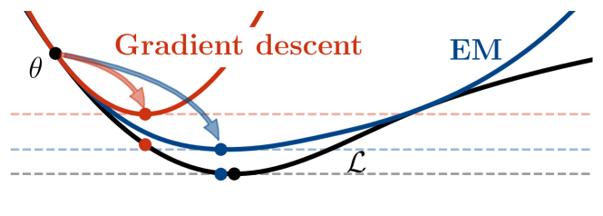
Figure 1: The surrogate optimized by EM is a tighter bound on the objective $\mathcal{L}$ than the quadratic bound implied by smoothness, optimized by gradient descent.

Since the development of EM and subsequent clarifications on the necessary conditions for convergence [11, 56], a large number of works have shown convergence results for EM and its many extensions, leading to a variety of insights about the algorithm, such as the effect of the ratio of missing information [57, 33] and the sample size [55, 59, 18, 5]. However, existing results on the global, non-asymptotic convergence of EM  rely on proof techniques developed for gradient descent on smooth functions, which rely on quadratic upper-bounds on the objective. Informally, this approach argues that the maximization step of the surrogate constructed by EM  does at least as well as gradient descent on a quadratic surrogate with a constant step-size, as illustrated in figure 1.

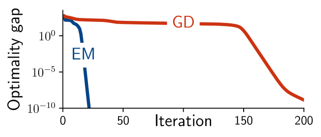
Figure 2: Performance of EM and gradient descent (GD) with constant step-size, selected by grid-search, for a Gaussian mixture model on the Old Faithful dataset. The large gap between the two methods suggests that existing theory for gradient descent is insufficient to explain the performance of EM.

The use of smoothness as a starting assumption leads to results that imply that EM behaves as a gradient method with a constant step-size. If true, there would be no difference between EM  and its gradient-based variants [29, e.g.]. This does not hold, however, and the resulting convergence rates are inevitably loose; EM makes more progress than this worst-case bound even on simple problems, as shown in figure 2.

Another issue is that, similarly to how Newton’s method is invariant to affine reparametrizations, EM is invariant to any homeomorphism [53]; the steps taken by EM are the same for any continuous, invertible reparametrization. This is not reflected by current analyses because the parametrization of the problem influences the smoothness of the function and the resulting convergence rate. For these reasons, the general frameworks proposed in the optimization literature [58, 34, 48, 45] where EM is a special case, do not reflect that EM is faster than typical members of these frameworks and yield loose analyses.

Most importantly, the assumption that the objective function is bounded by a quadratic does not hold in general. Results relying on smoothness do not apply, for example, to the standard textbook illustration of EM: Gaussian mixtures with learned covariance matrices [9, 38]. This is shown in figure 3. The smoothness assumption might be a reasonable simplification for local analyses, as it only needs to hold over a small subspace of the parameter space. In this setting, it does not detract from the main contribution of works investigating statistical properties or large-sample behavior. It does not hold, however, for global convergence analyses with arbitrary initializations. Our focus in this work is analyzing the classic EM algorithm when run for a finite number of iterations on a finite dataset, the setting in which people have been using EM for over 40 years and continue to use today.

We focus on the application of EM to exponential family models, of which Gaussian mixtures are a special case. Exponential families are by far the most common setting and an important special case as the M-step has a closed form solution. Modern stochastic and online extension of EM also rely on the form of exponential families to efficiently summarize past data [39, 51, 19].

The main tool for the analysis is the Kullback-Leibler (KL) divergence to describe distances between parameters. This approach was initially used to derive asymptotic convergence results [17, 16, 52] and to describe extensions of EM or EM-like algorithms [6, 12, 4, e.g.]. But it has not yet been applied to non-asymptotic convergence analyses. By using the KL divergence between the distributions rather than the Euclidean distance between their parameters, the results do not rely on invalid smoothness assumptions and are invariant to the choice of parametrization.

Focusing on convergence to a stationary point, as the EM objective $\mathcal{L}$ is non-convex, an informal summary of the main difference between previous analyses using smoothness and our results is that, after $T$ iterations,

Smoothness:	$\!\!\min_{t\leq T}\mathopen{}\mathclose{{}\left\|\mathop{}\!\nabla\mkern-2.0mu\mathcal{L}(\theta_{t})}\right\|^{2}$	$\!\!\!\!\!\!\leq\!\!\!\!\!\!$	$L\frac{\mathcal{L}(\theta_{1})-\mathcal{L}^{*}}{T}$
KL divergence:	$\!\!\min_{t\leq T}\mathrm{KL}{\mathopen{}\mathclose{{}\left[\mkern 1.0mu\theta_{t+1}\mkern 1.0mu\middle\|\mkern 1.0mu\theta_{t}\mkern 1.0mu}\right]}$	$\!\!\!\!\!\!\leq\!\!\!\!\!\!$	$\hphantom{L}\frac{\mathcal{L}(\theta_{1})-\mathcal{L}^{*}}{T}$

where $\mathcal{L}^{*}$ is the optimal value of the objective, $\mathcal{L}(\theta_{1})-\mathcal{L}^{*}$ is the initial optimality gap and $L$ is the smoothness constant. For non-smooth models, such as Gaussians with learned covariances (Fig. 3), $L=\infty$ and the bound is vacuous, whereas bounds in KL divergence do not depend on problem-specific constants. We show how the KL divergence relates to stationarity conditions for non-degenerate problems in section 5.

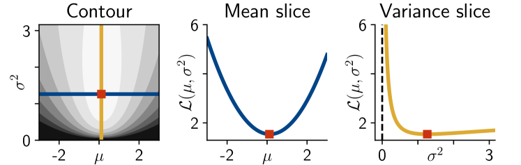
Figure 3: An exponential family distribution that cannot be smooth; fitting a Gaussian $\mathop{\mathcal{N}}\mathopen{}\mathclose{{}\left(\mu,\sigma^{2}}\right)$, including its variance. As the loss diverges to $\infty$, the objective cannot be upper-bounded by a quadratic function.

The key observation for exponential families is that M-step iterations match the moments of the model to the sufficient statistics of the data. We show that in this setting, EM can be interpreted as a mirror descent update, where each iteration minimizes the linearization of the objective and a KL divergence penalization term (rather than the gradient descent update which uses the Euclidean distance between parameters instead). While the connection between EM and exponential families is far from new, as it predates the codification of EM by [20] [10, eg,], the further connection to mirror descent to describe its behavior is, to the best of our knowledge, not acknowledged in the literature. More closely related to general optimization, our work can be seen as an application of the recent perspective of mirror descent as defining smoothness relative to a reference function, as presented by [7, 32].

Our main results are that we:

• Show that EM for the exponential family is a mirror descent algorithm, and that the EM objective is relatively smooth in KL divergence.

• Show the first homeomorphic-invariant non-asymptotic EM convergence rate, and how the KL divergence between iterates is related to stationary points and the natural gradient.

• Show how the ratio of missing information affects the non-asymptotic linear (or superlinear) convergence rate of EM around minimizers.

• Extend the results to generalized EM, where the M-step is only solved approximately.

• Discuss how to handle cases where the M-step is not in the exponential family (and might be non-differentiable) by analyzing the E-step.

2 EXPECTATION-MAXIMIZATION AND EXPONENTIAL FAMILIES

Before stating our results, we introduce the EM algorithm and necessary background on exponential families. For completeness, we provide additional details in appendix A and refer the reader to [54] for a full treatment of the subject.

EM applies when we want to maximize the likelihood $p(x\,|\,\theta)$ of data $x$ given parameters $\theta$, where the likelihood depends on unobserved variables $z$. By marginalizing over $z$, we obtain the negative log-likelihood (NLL), that we want to minimize (to maximize the likelihood), where $p(x,z\,|\,\theta)$ is the complete-data likelihood. The integral here is multi-dimensional if $z$ is, and a summation for discrete values, but we write all cases as a single integral for simplicity. EM is most useful when the complete-data NLL, $-\log p(x,z\,|\,\theta)$, is a convex function of $\theta$ and solvable in closed form if $z$ were known. EM defines the surrogate $Q_{\mkern-0.5mu\theta\mkern-0.5mu}(\phi)$, which estimates $\mathcal{L}(\phi)$ using the expected values for the latent variables at $\theta$,

$$Q_{\mkern-0.5mu\theta\mkern-0.5mu}(\phi)=-\raisebox{1.00006pt}{$\mkern-1.0mu\displaystyle\scaleobj{0.8}{\int}\mkern-1.0mu$}\log p(x,z\,|\,\phi)\,p(z\,|\,x,\theta)\operatorname{d\!}{z},$$

and iteratively updates $\theta_{t+1}\in\operatorname*{arg\,min}_{\phi}Q_{\mkern-0.5mu\theta_{t}\mkern-0.5mu}(\phi)$. The computation of the surrogate $Q_{\mkern-0.5mu\theta\mkern-0.5mu}(\cdot)$ and its minimization are typically referred to as the E-step and M-step.

A useful decomposition of the surrogate, shown by [20], is the equality

$$\begin{aligned} &Q_{\mkern-0.5mu\theta\mkern-0.5mu}(\phi)=\mathcal{L}(\phi)+H_{\mkern-0.5mu\theta\mkern-0.5mu}(\phi),\\ &\text{where }H_{\mkern-0.5mu\theta\mkern-0.5mu}(\phi)=-\raisebox{1.00006pt}{$\mkern-1.0mu\displaystyle\scaleobj{0.8}{\int}\mkern-1.0mu$}\log p(z\,|\,x,\phi)\,p(z\,|\,x,\theta)\operatorname{d\!}{z}\end{aligned}$$ (1)

is an entropy-like term minimized at $\phi=\theta$. That is,

$$H_{\mkern-0.5mu\theta\mkern-0.5mu}(\theta)\leq H_{\mkern-0.5mu\theta\mkern-0.5mu}(\phi) \mathop{}\!\nabla H_{\mkern-0.5mu\theta\mkern-0.5mu}(\theta)=0.$$ and

This gives two fundamental results about EM. Up to a constant, the surrogate is an upper-bound on the objective and improvement on $Q_{\theta}$ translates to improvement on $\mathcal{L}$, and the gradients of the loss and the surrogate match at the point it is formed, $\mathop{}\!\nabla Q_{\mkern-0.5mu\theta\mkern-0.5mu}(\theta)=\mathop{}\!\nabla\mkern-2.0mu\mathcal{L}(\theta)$.

2.1 Exponential families

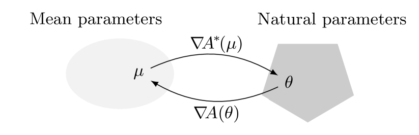
Figure 4: The gradient of the log-partition function and its dual, $(\mathop{}\!\nabla A,\mathop{}\!\nabla\mkern-2.0muA^{\mkern-1.0mu*}\mkern-1.0mu)$, form a bijection between the natural and mean parameters $\theta,\mu$.

Many canonical applications of EM, including mixture of Gaussians, are special cases where the complete-data distribution, given a value for the latent variable $z$, is an exponential family distribution;

$$\begin{aligned} p(x,z\,|\,\theta)&\propto\exp\mathopen{}\mathclose{{}\left(\mathopen{}\mathclose{{}\left\langle S(x,z),\theta}\right\rangle-\mkern-2.0muA(\theta)}\right),\end{aligned}$$ (2)

where $S$, $\theta$, and $\mkern-2.0muA$ are the sufficient statistics, natural parameters, and log-partition function of the distribution. Exponential family models are an important special case as the M-step has a closed form solution, and the update depends on the data only through the sufficient statistics. The solution for the maximum likelihood estimate (MLE) given $x$ and $z$ can be found from the stationary point of the complete log-likelihood,

$$\mathop{}\!\nabla\log p(x,z\,|\,\theta)=S(x,z)-\mathop{}\!\nabla\mkern-2.0muA(\theta)=0.$$ (3)

The gradient $\mathop{}\!\nabla\mkern-2.0muA$ yields the expected sufficient statistics, $\mathop{}\!\nabla\mkern-2.0muA(\theta)=\mathbb{E}\,\raisebox{-1.00006pt}{$\scriptstyle p(x,z\,|\,\theta)$}[S(x,z)]$, also called mean parameters and denoted by $\mu$. The log-partition function defines a bijection between the natural and mean parameters. Its inverse is given by $\mathop{}\!\nabla\mkern-2.0muA^{\mkern-1.0mu*}\mkern-1.0mu$, the gradient of the convex conjugate of $\mkern-2.0muA$, $\mkern-2.0muA^{\mkern-1.0mu*}\mkern-1.0mu(\mu)=\sup_{\theta}\mathopen{}\mathclose{{}\left\{\mathopen{}\mathclose{{}\left\langle\theta,\mu}\right\rangle-\mkern-2.0muA(\theta)}\right\},$ such that $\mu=\mathop{}\!\nabla\mkern-2.0muA(\theta)$ and $\theta=\mathop{}\!\nabla\mkern-2.0muA^{\mkern-1.0mu*}\mkern-1.0mu(\mu)$, as illustrated in figure 4. The solution to equation 3, given by

$$\mathop{}\!\nabla\mkern-2.0muA(\theta)=S(x,z) \implies \theta=\mathop{}\!\nabla\mkern-2.0muA^{\mkern-1.0mu*}\mkern-1.0mu(S(x,z)),$$

is called moment matching as its finds the parameter that, in expectation, generates the observed statistics.

To connect EM and mirror descent, we use the Bregman divergence induced by a convex function $h$; the difference between the function and its linearization,

$$D_{h}(\phi,\theta)=h(\phi)-h(\theta)-\mathopen{}\mathclose{{}\left\langle\mathop{}\!\nabla h(\theta),\phi-\theta}\right\rangle.$$ (4)

For exponential families, the Bregman divergence induced by the log-partition $\mkern-2.0muA$ is the KL divergence

$$D_{\mkern-1.0mu\mkern-2.0muA\mkern-1.0mu}(\phi,\theta)=\mathrm{KL}{\mathopen{}\mathclose{{}\left[\mkern 1.0mup(x,z\,|\,\theta)\mkern 1.0mu\middle\|\mkern 1.0mup(x,z\,|\,\phi)\mkern 1.0mu}\right]}.$$

The Bregman divergences induced by $\mkern-2.0muA$ and its conjugate $\mkern-2.0muA^{\mkern-1.0mu*}\mkern-1.0mu$ have the following relation (note the ordering)

$$D_{\mkern-1.0mu\mkern-2.0muA\mkern-1.0mu}(\phi,\theta)=D_{\mkern-1.0mu\mkern-2.0muA^{\mkern-1.0mu*}\mkern-1.0mu\mkern-1.0mu}(\mathop{}\!\nabla\mkern-2.0muA(\theta),\mathop{}\!\nabla\mkern-2.0muA(\phi)).$$ (5)

Both expressions are the same KL divergence, but differ in the parametrization used to express the distributions.

3 EM AND MIRROR DESCENT

Although EM iterations strictly decrease in the objective function if such decrease is possible locally, this does not directly imply convergence to stationary points, even asymptotically [11, 56]. The progress at each step could decrease faster than the objective. Characterizing the progress to ensure convergence requires additional assumptions.

Local analyses typically assume that the EM update contracts the distance to a local minima $\theta^{*}\!$,

$$\mathopen{}\mathclose{{}\left\|\theta_{t+1}-\theta^{*}}\right\|\leq c\mathopen{}\mathclose{{}\left\|\theta_{t}-\theta^{*}}\right\|,$$

for some $c<1$. On the other hand, global analyses typically assume the surrogate is smooth, meaning that

$$\mathopen{}\mathclose{{}\left\|\mathop{}\!\nabla Q_{\mkern-0.5mu\bm{\cdot}\mkern-0.5mu}(\theta)-\mathop{}\!\nabla Q_{\mkern-0.5mu\bm{\cdot}\mkern-0.5mu}(\phi)}\right\|\leq L\mathopen{}\mathclose{{}\left\|\theta-\phi}\right\|.$$

for all $\theta$ and $\phi$, and some fixed constant $L$. This is equivalent to assuming the following upper bound holds,

$$\mathcal{L}(\phi)\leq\mathcal{L}(\theta)+\mathopen{}\mathclose{{}\left\langle\mathop{}\!\nabla\mkern-2.0mu\mathcal{L}(\theta),\phi-\theta}\right\rangle+\frac{L}{2}\mathopen{}\mathclose{{}\left\|\theta-\phi}\right\|^{2}.$$

While the local analyses assumptions are reasonable, the worst-case value of $L$ for global results can be infinite, as in the simple example of figure 3. Instead, we show that the following upper-bound in KL divergence holds without additional assumptions.

Proposition 1.

For exponential family distributions, the M-step update in Expectation-Maximization is equivalent to the minimization of the following upper-bound;

$$\mathcal{L}(\phi)\leq\mathcal{L}(\theta)+\mathopen{}\mathclose{{}\left\langle\mathop{}\!\nabla\mkern-2.0mu\mathcal{L}(\theta),\phi-\theta}\right\rangle+D_{\mkern-1.0mu\mkern-2.0muA\mkern-1.0mu}(\phi,\theta),$$ (6)

where $\mkern-2.0muA$ is the log-partition of the complete-data distribution, and $D_{\mkern-1.0mu\mkern-2.0muA\mkern-1.0mu}(\phi,\theta)=\mathrm{KL}{\mathopen{}\mathclose{{}\left[\mkern 1.0mup(x,z\,|\,\theta)\mkern 1.0mu\middle\|\mkern 1.0mup(x,z\,|\,\phi)\mkern 1.0mu}\right]}$.

While the upper bound is still expressed in a specific parametrization to describe the distributions, the KL divergence is a property of the distributions, independent of their representation. As this upper-bound is the one minimized by the M-step, it is a direct description of the algorithm rather than an additional surrogate used for convenience, as was illustrated in figure 1.

This gives an interpretation of EM in terms of the mirror descent algorithm [41, 8], the minimization of a first-order Taylor expansion and Bregman divergence as in equation 6, with step-size $\alpha\mkern-1.0mu=\mkern-1.0mu1$. In the recent perspective of mirror descent framed as relative smoothness [7, 32], the objective function is 1-smooth relative to $\mkern-2.0muA$. Existing results [32, e.g.] then directly imply the following local result, up to non-degeneracy assumptions A1–A3 discussed in the next section.

Corollary 1.

For exponential families, if EM is initialized in a locally-convex region with minimum $\theta^{*}\!$,

$$\mathcal{L}(\theta_{T})-\mathcal{L}(\theta^{*})\leq\frac{1}{T}\,\mathrm{KL}{\mathopen{}\mathclose{{}\left[\mkern 1.0mup(x,z\,|\,\theta_{1})\mkern 1.0mu\middle\|\mkern 1.0mup(x,z\,|\,\theta^{*})\mkern 1.0mu}\right]}.$$ (7)

This is the first non-asymptotic convergence rate for EM that does not depend on problem-specific constants.

Proof of proposition 1.

Recall the decomposition of the surrogate in terms of the objective and entropy term, $Q_{\mkern-0.5mu\theta\mkern-0.5mu}(\phi)=\mathcal{L}(\phi)+H_{\mkern-0.5mu\theta\mkern-0.5mu}(\phi)$ in equation 1. It gives

$$\mathcal{L}(\phi)-\mathcal{L}(\theta)=Q_{\mkern-0.5mu\theta\mkern-0.5mu}(\phi)-Q_{\mkern-0.5mu\theta\mkern-0.5mu}(\theta)+H_{\mkern-0.5mu\theta\mkern-0.5mu}(\theta)-H_{\mkern-0.5mu\theta\mkern-0.5mu}(\phi),$$

where $H_{\mkern-0.5mu\theta\mkern-0.5mu}(\theta)-H_{\mkern-0.5mu\theta\mkern-0.5mu}(\phi)\leq 0$ as $H_{\mkern-0.5mu\theta\mkern-0.5mu}(\phi)$ is minimized at $\phi=\theta$. We will show that for exponential families,

$$Q_{\mkern-0.5mu\theta\mkern-0.5mu}(\phi)-Q_{\mkern-0.5mu\theta\mkern-0.5mu}(\theta)=\mathopen{}\mathclose{{}\left\langle\mathop{}\!\nabla\mkern-2.0mu\mathcal{L}(\theta),\phi-\theta}\right\rangle+D_{\mkern-1.0mu\mkern-2.0muA\mkern-1.0mu}(\phi,\theta),$$

which implies the upper-bound in equation 6 and that its minima matches that of $Q_{\mkern-0.5mu\theta\mkern-0.5mu}(\phi)$.

If the complete-data distribution is in the exponential family, the surrogate in natural parameters is

$$\begin{aligned} Q_{\mkern-0.5mu\theta\mkern-0.5mu}(\phi)&=-\raisebox{1.00006pt}{$\mkern-1.0mu\displaystyle\scaleobj{0.8}{\int}\mkern-1.0mu$}\log p(x,z\,|\,\phi)\,p(z\,|\,x,\theta)\operatorname{d\!}{z},\\[-5.0pt] &=-\raisebox{1.00006pt}{$\mkern-1.0mu\displaystyle\scaleobj{0.8}{\int}\mkern-1.0mu$}\mathopen{}\mathclose{{}\left[\mathopen{}\mathclose{{}\left\langle S(x,z),\phi}\right\rangle-\mkern-2.0muA(\phi)}\right]\,p(z\,|\,x,\theta)\operatorname{d\!}{z},\\ &=-\mathopen{}\mathclose{{}\left\langle\textstyle\operatorname*{\mathbb{E}}_{p(z\,|\,x,\theta)}\mathopen{}\mathclose{{}\left[S(x,z)}\right],\phi}\right\rangle+\mkern-2.0muA(\phi).\end{aligned}$$ (8)

Using $s(\theta)=\operatorname*{\mathbb{E}}_{p(z\,|\,x,\theta)}\mathopen{}\mathclose{{}\left[S(x,z)}\right]$ for the expected sufficient statistics and expanding $Q_{\mkern-0.5mu\theta\mkern-0.5mu}(\phi)-Q_{\mkern-0.5mu\theta\mkern-0.5mu}(\theta)$ yields

$$Q_{\mkern-0.5mu\theta\mkern-0.5mu}(\phi)-Q_{\mkern-0.5mu\theta\mkern-0.5mu}(\theta) =-\mathopen{}\mathclose{{}\left\langle s(\theta),\phi-\theta}\right\rangle+\mkern-2.0muA(\phi)-\mkern-2.0muA(\theta),$$

$$\stackrel{{\scriptstyle{(1)}}}{{=}}-\mathopen{}\mathclose{{}\left\langle s(\theta)-\mathop{}\!\nabla\mkern-2.0muA(\theta),\phi-\theta}\right\rangle+D_{\mkern-1.0mu\mkern-2.0muA\mkern-1.0mu}(\phi,\theta),$$

$$\stackrel{{\scriptstyle{(2)}}}{{=}}\mathopen{}\mathclose{{}\left\langle\mathop{}\!\nabla\mkern-2.0mu\mathcal{L}(\theta),\phi-\theta}\right\rangle+D_{\mkern-1.0mu\mkern-2.0muA\mkern-1.0mu}(\phi,\theta),$$

where $\scriptstyle{(1)}$ adds and subtracts $\mathopen{}\mathclose{{}\left\langle\mathop{}\!\nabla\mkern-2.0muA(\theta),\phi-\theta}\right\rangle$ to complete the Bregman divergence and $\scriptstyle{(2)}$ uses that the gradient of the surrogate and the objective match at $\theta$,

$$\mathop{}\!\nabla\mkern-2.0mu\mathcal{L}(\theta)=\mathop{}\!\nabla Q_{\mkern-0.5mu\theta\mkern-0.5mu}(\theta)=\mathop{}\!\nabla\mkern-1.0mu\mkern-2.0muA(\theta)-s(\theta).$$ ∎

This perspective extends to stochastic approximation [49] variants of EM, which are becoming increasingly relevant as they scale to large datasets. Algorithms such as incremental, stochastic and online EM [39, 51, 13] average the observed sufficient statistics to update the parameters. This can be cast as stochastic mirror descent [40] with step-sizes decreasing as $\nicefrac{{1}}{{t}}$. For brevity, we leave the derivation to appendix B.

4 ASSUMPTIONS AND OPEN CONSTRAINTS

Before diving into convergence results, we discuss the assumptions needed for the method to be well defined.

1. The complete-data distribution $p(x,z\,|\,\theta)$ is a steep, minimal exponential family distribution.

A1 implies the continuity and differentiability of $\mathcal{L}$, that the surrogate has a unique solution, and that the natural and mean parameters are well defined. It is the statistical equivalent to the assumption in the mirror descent literature that $\mkern-2.0muA$ essentially smooth, which implies that the mappings $\mathop{}\!\nabla\mkern-2.0muA,\mathop{}\!\nabla\mkern-2.0muA^{\mkern-1.0mu*}\mkern-1.0mu$ are well-defined. A1 is satisfied in the most commons applications of EM in machine learning, including Gaussian mixtures.

The next assumptions deal with a further subtle issue that arises when we attempt to apply results from the optimization literature to EM, like the generic frameworks of [58], [34] or [48]. The parameters of the distributions optimized by EM are typically constrained to a subset $\theta\in\Omega$, like that probabilities sum to one and that covariance matrices are positive-definite. To handle constraints, those analyses assume access to a projection onto the constraint set $\Omega$. However, this does not hold for common settings of EM like mixtures of Gaussians. When the boundaries of the constraint set are open, the projection operator does not exist (there is no “closest positive-definite matrix” to a matrix that is not positive-definite). An additional complication is related to the existence of a lower-bound on the objective. For example, in Gaussian mixtures, we can drive the objective to $\scalebox{0.75}[1.0]{$-$}\infty$ by centering a Gaussian on a single data point and shrinking the variance towards zero. The existence of such degenerate solutions is challenging for non-asymptotic convergence rates, as results typically depend on the optimality gap $\mathcal{L}(\theta)-\mathcal{L}^{*}$ and are vacuous if it is unbounded. To avoid those degenerate cases, we make the following assumptions.

1. The objective function is lower-bounded by some $\mathcal{L}^{*}>\scalebox{0.75}[1.0]{$-$}\infty$ on the constraint set $\Omega$.

1. The sub-level sets $\Omega_{\theta}=\{\phi\in\Omega:Q_{\mkern-0.5mu\theta\mkern-0.5mu}(\phi)\leq Q_{\mkern-0.5mu\theta\mkern-0.5mu}(\theta)\}$ are compact (closed and bounded).

One approach to ensure the EM updates are well-defined is to add regularization, in the form of a proper conjugate prior. If the parameters approach the boundary (or diverge in an unbounded direction), the prior acts as a barrier and diverges to $\infty$ rather than $\scalebox{0.75}[1.0]{$-$}\infty$. The minimum of the surrogate is then finite and in $\Omega$ at every iteration, without the need for projections. This is illustrated in figure 5. For simplicity of presentation, we assume A2 and A3 hold and discuss maximum a posteriori (MAP) estimation in appendix C.

Figure 5: Example of a barrier function with compact sub-level sets on an open set $\Omega$, satisfying A2 and A3. Even if $\Omega$ is open, as $f$ goes to $\infty$ at the boundary and is convex, the minimum is guaranteed to be in $\Omega$.

5 CONVERGENCE OF EM FOR EXPONENTIAL FAMILIES

We now give the main results for the convergence of EM to stationary points for exponential families. This analysis takes advantage of existing tools for the analysis of mirror descent, but in the less-common non-convex setting. Detailed proofs are deferred to appendix D.

Proposition 2.

Under assumptions A1–A3, EM for exponential family distributions converges at the rate

$$\min_{t\leq T}\,\mathrm{KL}{\mathopen{}\mathclose{{}\left[\mkern 1.0mup(x,z\,|\,\theta_{t+1})\mkern 1.0mu\middle\|\mkern 1.0mup(x,z\,|\,\theta_{t})\mkern 1.0mu}\right]}\leq\frac{\mathcal{L}(\theta_{1})-\mathcal{L}^{*}}{T}.$$

While this result implies the distribution fit by EM stops changing, it does not—in itself—guarantee progress toward a stationary point as it is also satisfied by an algorithm that does not move, $\theta_{t+1}\mkern-1.0mu=\theta_{t}$. In the standard setting of gradient descent with constant step-size, proposition 2 is the equivalent of the statement that the distance between iterates $\|\theta_{t+1}-\theta_{t}\|$ converges. As $\|\theta_{t+1}-\theta_{t}\|\mkern-2.0mu\propto\mkern-2.0mu\|\mathop{}\!\nabla\mkern-2.0mu\mathcal{L}(\theta_{t})\|$, it also implies that the gradient norm converges. A similar result holds for EM, where measuring distances between iterates with $D_{\mkern-1.0mu\mkern-2.0muA\mkern-1.0mu}$ leads to stationarity in the dual divergence $D_{\mkern-1.0mu\mkern-2.0muA^{\mkern-1.0mu*}\mkern-1.0mu\mkern-1.0mu}$.

Recall that the M-step finds a stationary point of the upper-bound in equation 6. Setting its derivative to 0, using $\mathop{}\!\nabla_{\mspace{-4.0mu}\phi}\,D_{\mkern-1.0mu\mkern-2.0muA\mkern-1.0mu}(\phi,\theta_{t})=\mathop{}\!\nabla\mkern-2.0muA(\phi)-\mathop{}\!\nabla\mkern-2.0muA(\theta_{t})$ yields

$$\mathop{}\!\nabla\mkern-2.0mu\mathcal{L}(\theta_{t})-\mathop{}\!\nabla\mkern-2.0muA(\theta_{t})+\mathop{}\!\nabla\mkern-2.0muA(\theta_{t+1})=0.$$

Using the expansion of the gradient in terms of the observed statistics $s(\theta_{t})$ and the mean parametrization $\mu_{t}=\mathop{}\!\nabla\mkern-2.0muA(\theta_{t})$, we obtain the moment matching update; finding the mean parameters $\mu_{t+1}$ that generate the observed sufficient statistics $s(\theta_{t})$ in expectation;

$$\mu_{t+1}=s(\theta_{t})=\mu_{t}-\mathop{}\!\nabla\mkern-2.0mu\mathcal{L}(\theta_{t}).$$

Expressing the KL divergence as the dual Bregman divergence $D_{\mkern-1.0mu\mkern-2.0muA^{\mkern-1.0mu*}\mkern-1.0mu\mkern-1.0mu}(\mu_{t+1},\mu_{t})$ (Equation 5) then gives

$$\begin{aligned} \mathrm{KL}{\mathopen{}\mathclose{{}\left[\mkern 1.0mu\theta_{t+1}\mkern 1.0mu\middle\|\mkern 1.0mu\theta_{t}\mkern 1.0mu}\right]}&=D_{\mkern-1.0mu\mkern-2.0muA^{\mkern-1.0mu*}\mkern-1.0mu\mkern-1.0mu}(\mu_{t+1},\mu_{t})=D_{\mkern-1.0mu\mkern-2.0muA^{\mkern-1.0mu*}\mkern-1.0mu\mkern-1.0mu}(s(\theta_{t}),\mu_{t}).\end{aligned}$$

This adds a measure of stationarity to proposition 2;

Corollary 2.

Under assumptions A1–A3,

$$\min_{t\leq T}\,D_{\mkern-1.0mu\mkern-2.0muA^{\mkern-1.0mu*}\mkern-1.0mu\mkern-1.0mu}(s(\theta_{t}),\mu_{t})\leq\frac{\mathcal{L}(\theta_{1})-\mathcal{L}^{*}}{T}.$$

The observed sufficient statistics $s(\theta_{t})$ and mean parameters $\mu_{t}$ are the two parts of the gradient, $\mathop{}\!\nabla\mkern-2.0mu\mathcal{L}(\theta_{t})=\mu_{t}-s(\theta_{t})$, and $D_{\mkern-1.0mu\mkern-2.0muA^{\mkern-1.0mu*}\mkern-1.0mu\mkern-1.0mu}(s(\theta_{t}),\mu_{t})=0$ implies $\mathop{}\!\nabla\mathcal{L}(\theta_{t})=0$.

corollary 2 is the Bregman divergence analog of the standard result for steepest descent in an arbitrary norm $\mathopen{}\mathclose{{}\left\|\cdot}\right\|$, giving convergence in the dual norm $\mathopen{}\mathclose{{}\left\|\mathop{}\!\nabla\mkern-2.0mu\mathcal{L}}\right\|_{*}$. If the smoothness assumption is satisfied with constant $L$, we recover existing results in Euclidean norm,

$$\min_{t\leq T}\,\mathopen{}\mathclose{{}\left\|\mathop{}\!\nabla\mkern-2.0mu\mathcal{L}(\theta_{t})}\right\|^{2}\leq\frac{L}{T}\mathopen{}\mathclose{{}\left(\mathcal{L}(\theta_{1})-\mathcal{L}^{*}}\right),$$

as the $L$-smoothness of $\mkern-2.0muA$ implies the $\nicefrac{{1}}{{L}}$-strong convexity of $\mkern-2.0muA^{\mkern-1.0mu*}\mkern-1.0mu$ and $D_{\mkern-1.0mu\mkern-2.0muA^{\mkern-1.0mu*}\mkern-1.0mu\mkern-1.0mu}(\mu_{t+1},\mu_{t})\geq\nicefrac{{1}}{{L}}\,\|\mathop{}\!\nabla\mkern-2.0mu\mathcal{L}(\theta_{t})\|{}^{2}$.

The convergence in KL divergence, however, does not depend on additional smoothness assumptions and is a stronger guarantee as it implies the probabilistic models being optimized stop changing. This can not be directly guaranteed by small gradient norms, as differences in distributions do not only depend on the difference between parameters. For example, how much a Gaussian distribution changes when changing the mean depends on its variance; if the variance is small, the change will be big, but if the variance is large, the change will be comparatively smaller. This is illustrated in figure 6, and is not captured by gradient norms.

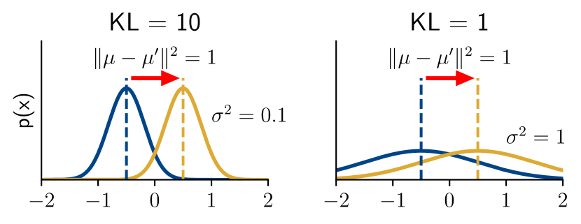
Figure 6: The similarity between two Gaussians depends on their variance, even if it is fixed. The Euclidean distance between parameters, and by extension gradient norms, is a poor measure of stationarity as it ignores unchanged parameters.

5.1 Connection to the Natural Gradient

A useful simplification to interpret the divergence is to consider the norm it is locally equivalent to. By a second-order Taylor expansion, we have that

$$D_{\mkern-1.0mu\mkern-2.0muA^{\mkern-1.0mu*}\mkern-1.0mu\mkern-1.0mu}(\mu+\delta,\mu)\approx\mathopen{}\mathclose{{}\left\|\delta}\right\|_{\mathop{}\!\nabla^{2}\mkern-2.0muA^{\mkern-1.0mu*}\mkern-1.0mu(\mu)}^{2},$$

where $\|\delta\|\raisebox{5.0pt}{$\scriptstyle 2$}\mkern-2.0mu\!\!\raisebox{-2.5pt}{$\scriptstyle\mathop{}\!\nabla^{2}\mkern-2.0muA^{\mkern-1.0mu*}\mkern-1.0mu(\mu)$}=\langle\delta,\mathop{}\!\nabla^{2}\mkern-2.0muA^{\mkern-1.0mu*}\mkern-1.0mu(\mu)\delta\rangle$. For exponential families, $\mathop{}\!\nabla^{2}\mkern-2.0muA^{\mkern-1.0mu*}\mkern-1.0mu$ is the inverse of the Fisher information matrix of the complete-data distribution $p(x,z\,|\,\theta)$,

$$\mathop{}\!\nabla^{2}\mkern-2.0muA^{\mkern-1.0mu*}\mkern-1.0mu(\mu)=I_{x,z}(\theta)^{-1}\mkern-2.0mu=\textstyle\operatorname*{\mathbb{E}}_{x,z\sim p(x,z\,|\,\theta)}\mathopen{}\mathclose{{}\left[\mathop{}\!\nabla^{2}\log p(x,z\,|\,\theta)}\right].$$

The left side of corollary 2 is then, locally,

$$D_{\mkern-1.0mu\mkern-2.0muA^{\mkern-1.0mu*}\mkern-1.0mu\mkern-1.0mu}(\mu_{t}-\mathop{}\!\nabla\mkern-2.0mu\mathcal{L}(\theta_{t}),\mu_{t})\approx\mathopen{}\mathclose{{}\left\|\mathop{}\!\nabla\mkern-2.0mu\mathcal{L}(\theta_{t})}\right\|_{I_{x,z}(\theta_{t})^{-1}}^{2}.$$ (9)

This quantity is the analog of the Newton decrement,

$$\mathopen{}\mathclose{{}\left\|\mathop{}\!\nabla\mkern-2.0mu\mathcal{L}(\theta_{t})}\right\|^{2}_{\mathop{}\!\nabla^{2}\mathcal{L}(\theta_{t})^{-1}},$$

used in the affine-invariant analysis of Newton’s method [43]. But equation 9 is for the natural gradient in information geometry, $I_{x,z}(\theta_{t})^{-1}\mathop{}\!\nabla\mkern-2.0mu\mathcal{L}(\theta_{t})$ [3]. While the Newton decrement is invariant to affine reparametrizations, this “natural decrement” is also invariant to any homeomorphism.

5.2 Invariant Local Linear Rates

It was already established by [20] that, asymptotically, the EM algorithm converges $r$-linearly, meaning that if it is in a convex region,

$$\mathcal{L}(\theta_{t+1})-\mathcal{L}^{*}\leq r(\mathcal{L}(\theta_{t})-\mathcal{L}^{*}) \text{ for }r<1,$$ (10)

near a strict minima $\theta^{*}$, where the rate $r$ is determined by the amount of “missing information”. In this section, we strengthen corollary 1 to show this result extends to local but non-asymptotic rates.

The improvement ratio $r$ is determined by the eigenvalues of the missing information matrix $M$ at $\theta^{*}$, defined as [44]

$$M(\theta^{*})=I_{x,z}(\theta^{*})^{-1}I_{z\,|\,x}(\theta^{*}),$$ (11)

where $I_{x,z}(\theta)$ and $I_{z\,|\,x}(\theta)$ are the Fisher information matrices of the complete-data distribution $p(x,z\,|\,\theta)$ and conditional missing-data distribution $p(z\,|\,x,\theta)$. Intuitively this matrix measures how much information is missing and how much easier the problem would be if we had access to the true values of the latent variables. If $I_{z\,|\,x}(\theta)$ is small, there is little information to be gained from observing the latent variables as most of this information is already contained in $x$. But $I_{z\,|\,x}(\theta)$ is high if the known values of $x$ do not constrain the possible values of $z$ and the problem is more difficult.

The matrix $M(\theta)$ is not a fixed quantity and evolves with the parameters $\theta$. In regions where we have a good model of the data, for example if we found well-separated clusters fit with Gaussian mixtures, there is little uncertainty about the latent variables (the cluster membership) and $M(\theta)$ will be small. However, $M(\theta)$ is often large at the start of the optimization procedure. The linear rate $r$ in equation 10 is then determined by the maximum eigenvalue of the missing information, $r=\lambda_{\max}\mathopen{}\mathclose{{}\left(M(\theta^{*})}\right)$. Linear convergence occurs if the missing information at $\theta^{*}$ is small, $M(\theta^{*})\prec 1$, otherwise $r$ can be larger than $1$.

This result, however, is only asymptotic and existing non-asymptotic linear rates rely on strong-convexity assumptions instead [5, e.g.]. A twice-differentiable function $f$ is $\alpha$-strongly convex if

$$\mathop{}\!\nabla^{2}f(\theta)\succeq\alpha I \text{for }\alpha>0,$$

which means the eigenvalues of $\mathop{}\!\nabla^{2}f(\theta)$ are bounded below by $\alpha$. If $f$ is also $L$-smooth, as defined in section 3, a gradient-EM type of analysis gives that

$$f(\theta_{t+1})-f^{*}\leq\mathopen{}\mathclose{{}\left(1-\frac{\alpha}{L}}\right)\mathopen{}\mathclose{{}\left(f(\theta_{t})-f^{*}}\right).$$

This implies EM converges linearly if it enters a smooth and strongly-convex region. However, in these works, the connection to the ratio of missing information is lost and the rate is not invariant to reparametrization.

We showed in section 3 that, instead of measuring smoothness in Euclidean norms, the EM objective is $1$-smooth relative to its log-partition function $\mkern-2.0muA$. Likewise, we can characterize strong convexity relative to a reference function $h$ [32], requiring that

$$\mathop{}\!\nabla^{2}\mathcal{L}(\theta)\succeq\alpha\mkern-1.0mu\mathop{}\!\nabla^{2}h(\theta) \text{ for }\alpha>0.$$ (12)

For EM, where we care about strong convexity relative to the log-partition $\mkern-2.0muA$, the relative strong-convexity parameter $\alpha$ is directly related to the missing information;

Proposition 3.

For exponential families, the EM objective is $\alpha$-strongly convex relative to $\mkern-2.0muA$ on a region $\Theta$ iff the missing information $M$ (Equation 11) satisfies

$$\lambda_{\max}(M(\theta))\leq(1-\alpha) \text{ for all }\theta\in\Theta.$$

We provide a detailed proof in appendix D and give here the main intuition. For exponential families, the Hessian of the surrogate $Q_{\mkern-0.5mu\theta\mkern-0.5mu}(\theta)$ coincides with the Hessian of $\mkern-2.0muA(\theta)$ (Equation 8), which is the Fisher information matrix of the complete-data distribution, $I_{x,z}(\theta)$. Using the decomposition of equation 1, the Hessian of the objective can be shown to be equal to

$$\mathop{}\!\nabla^{2}\mathcal{L}(\theta)=I_{x,z}(\theta)-I_{z\,|\,x}(\theta).$$

The definition of $\alpha$-strong convexity relative to $\mkern-2.0muA$ (Equation 12) for EM is then equivalent to

$$I_{x,z}(\theta)-I_{z\,|\,x}(\theta)\succeq\alpha I_{x,z}(\theta).$$

Multiplying by $I_{x,z}(\theta)^{-1}$ and rearranging terms yields

$$M(\theta)=I_{x,z}(\theta)^{-1}I_{z\,|\,x}(\theta)\preceq(1-\alpha)I.$$ ∎

Convergence results for mirror descent on relatively $1$-smooth and $\alpha$-strongly convex functions [32] then directly give the following local linear rate.

Corollary 3.

Under A1–A3, if EM is initialized in a locally convex region $\Theta$ with minimum $\mathcal{L}^{*}$ and the ratio of missing information is bounded, $\lambda_{\max}(M(\theta))\leq r$,

$$\mathcal{L}(\theta_{t+1})-\mathcal{L}^{*}\leq r\mathopen{}\mathclose{{}\left(\mathcal{L}(\theta_{t})-\mathcal{L}^{*}}\right).$$

If the ratio of missing information goes to zero, as in the case of well-separated clusters for Gaussian mixtures with suitable initialization, then EM converges superlinearly in the neighborhood of a solution [50, 57, 33].

5.3 Generalized EM

We now consider generalized EM schemes, which do not optimize the surrogate exactly in the M-step but output an approximate (possibly randomized) update. Given $\theta_{t}$, we assume we can solve the surrogate problem with some expected guarantee on the optimality gap, $\operatorname*{\mathbb{E}}\mathopen{}\mathclose{{}\left[Q_{\mkern-0.5mu\theta_{t}\mkern-1.0mu\mkern-0.5mu}(\theta_{t+1})-Q_{\mkern-0.5mu\theta_{t}\mkern-1.0mu\mkern-0.5mu}^{*}}\right]$, where $Q_{\mkern-0.5mu\theta_{t}\mkern-1.0mu\mkern-0.5mu}^{*}$ is the minimum value of the surrogate. The M-step achieve $Q_{\mkern-0.5mu\theta_{t}\mkern-1.0mu\mkern-0.5mu}(\theta_{t+1})=Q_{\mkern-0.5mu\theta_{t}\mkern-1.0mu\mkern-0.5mu}^{*}$, but it might be more efficient to solve the problem only partially, or the M-step might be intractable. We consider two types of guarantees for those two cases, multiplicative and additive errors.

1. Multiplicative error: The approximate solution $\theta_{t+1}$ satisfies the guarantee that, for some $c\mkern-1.0mu\in\mkern-1.0mu(0,1]$,

$$\operatorname*{\mathbb{E}}\mathopen{}\mathclose{{}\left[Q_{\mkern-0.5mu\theta_{t}\mkern-1.0mu\mkern-0.5mu}(\theta_{t+1})-Q_{\mkern-0.5mu\theta_{t}\mkern-1.0mu\mkern-0.5mu}^{*}}\right]\leq(1-c)\mathopen{}\mathclose{{}\left(Q_{\mkern-0.5mu\theta_{t}\mkern-1.0mu\mkern-0.5mu}(\theta_{t})-Q_{\mkern-0.5mu\theta_{t}\mkern-1.0mu\mkern-0.5mu}^{*}}\right).$$

If $c=1$, the algorithm is exact and $\theta_{t+1}$ minimizes the surrogate, while for $c=0$ there is no guarantee of progress. An example of an algorithm satisfying this condition for mixture models would be the exact optimization of only one of the mixture components, chosen at random, like the ECM algorithm of [37]. As the surrogate problem is separable among components, the guarantee is satisfied with $c=\nicefrac{{1}}{{k}}$, where $k$ is the number of clusters.

Theorem 1.

Under assumptions A1–A3, if the M-steps are solved up to $c$-multiplicative error (A4),

$$\min_{t\leq T}\,\operatorname*{\mathbb{E}}\mathopen{}\mathclose{{}\left[D_{\mkern-1.0mu\mkern-2.0muA^{\mkern-1.0mu*}\mkern-1.0mu\mkern-1.0mu}(s(\theta_{t}),\mu_{t})}\right]\leq\frac{1}{c}\frac{\mathcal{L}(\theta_{1})-\mathcal{L}^{*}}{T}.$$

This can give speedup in overall time if some iterations can be made more than than $c$ times faster by leveraging the structure of the problem.

Multiplicative error, however, is a strong assumption if the closed-form solution is intractable. Instead, additive error is almost always satisfied. For example, although suboptimal for the reasons mentioned earlier, running GD with a line-search on the surrogate guarantees additive error if the objective is (locally) smooth.

1. Additive error: The algorithm returns a solution $\theta_{t+1}$ with the guarantee that, in expectation,

$$\operatorname*{\mathbb{E}}\mathopen{}\mathclose{{}\left[Q_{\mkern-0.5mu\theta_{t}\mkern-1.0mu\mkern-0.5mu}(\theta_{t+1})-Q_{\mkern-0.5mu\theta_{t}\mkern-1.0mu\mkern-0.5mu}^{*}}\right]\leq\epsilon_{t}.$$

If $\epsilon_{t}=0$, the optimization is exact. Otherwise, the algorithm might not guarantee progress and the sequence $\epsilon_{t}$ needs to converge to 0 for the iterations to converge.

Theorem 2.

Under assumptions A1–A3, if the M-step at step $t$ is solved up to $\epsilon_{t}$-additive error (A5),

$$\min_{t\leq T}\,\operatorname*{\mathbb{E}}\mathopen{}\mathclose{{}\left[D_{\mkern-1.0mu\mkern-2.0muA^{\mkern-1.0mu*}\mkern-1.0mu\mkern-1.0mu}(s(\theta_{t}),\mu_{t})}\right]\leq\frac{\mathcal{L}(\theta_{1})-\mathcal{L}^{*}}{T}+\frac{1}{T}\sum_{t=1}^{T}\epsilon_{t}.$$

For example, for $\epsilon_{t}=\mathop{\mathcal{O}}(1/t)$, the rate reduces to $\mathop{\mathcal{O}}(\log(T)/T)$, but we recover a $\mathop{\mathcal{O}}(1/T)$ rate if the errors decrease faster, $\epsilon_{t}=\mathop{\mathcal{O}}(1/t^{2})$. As in section 5.2, the results can be extended to give convergence in function values in a locally convex region. The proofs of theorems 1 and 2 are deferred to appendix D.

5.4 EM for General Models

While the exponential family covers many applications of EM, some are not smooth, in Euclidean distance or otherwise. For example, in a mixture of Laplace distributions the gradient of the surrogate is discontinuous (the Laplace distribution is not an exponential family). In this case, the progress of the M-step need not be related to the gradient and results similar to corollary 2 do not hold. To the best of our knowledge, there are no general non-asymptotic convergence results for the general non-differentiable, non-convex setting and all we can guarantee is asymptotic convergence, as in the works of [16, 52].

The tools presented here can still obtain partial answers for the Laplace mixture and similar examples. The analyses in previous sections considered the progress of the M-step, as is common in non-asymptotic literature. We can instead view the E-step as the primary driver of progress, as is more common in the asymptotic literature. Assuming relative smoothness on the conditional distribution $p(z\,|\,x,\theta)$ only, we derive in appendix E an analog of corollary 2 for stationarity on the latent variables, rather than the complete-data distribution. This guarantee is weaker, but the assumption holds more generally. For example, it is satisfied by any finite mixture, even if the mixture components are non-differentiable, as for the Laplace mixture.

6 DISCUSSION

Instead of assuming that the objective is smooth in Euclidean norm and applying the methodology for the convergence of gradient descent, which does not hold even for the standard Gaussian mixture examples found in textbooks, we showed that EM for exponential families always satisfies a notion of smoothness relative to a Bregman divergence. In this setting, EM and its stochastic variants are equivalent to mirror descent updates. This perspective leads to convergence rates that hold without additional assumptions and that are invariant to reparametrization. We also showed how the ratio of missing information can be integrated in non-asymptotic convergence rates, and analyzed the use of approximate M-steps. Although we focused on the MLE, appendix C discusses MAP estimation. We show that results similar to proposition 2 on the convergence to stationary points in KL divergence still hold, with minor changes to incorporate the prior. Viewing EM as a mirror descent procedure also highlights that it is a first-order method. It is thus susceptible to similar issues as classical first-order methods, such as slow progress in “flat” regions. However, flatness is measured in a different geometry (KL divergence) rather than the Euclidean geometry of gradient descent.

Beyond non-asymptotic convergence, smoothness relative to a KL divergence could be applied to extend statistical results, such as that of [18] to settings other than well-separated mixtures of Gaussians. In addition to the EM algorithm, our results could be extended to variational methods, such as the works of [24, 28], due to the similarity between the EM surrogate and the evidence lower-bound.

Stochastic variants of EM are becoming increasingly relevant as they allow the algorithm to scale to large datasets, and recent recent work by [15, 27] combined stochastic EM updates with variance reduction methods like SAG, SVRG, and MISO [31, 25, 35]. But the analysis in those works take the view of EM as a preconditioned gradient step. The resulting worst-case analysis not only depends on the smoothness constant, but the prescribed step-size is proportional to $\nicefrac{{1}}{{L}}$. For Gaussian mixtures with arbitrary initialization, this implies using a step-size of 0. Our results highlights the gap between EM and gradient-EM methods, using a combination of classic and modern tools from a variety of fields, and we hope that the tools developed here may help to fix this and similar practical issues.

Acknowledgements

We thank the anonymous reviewers, whose comments helped improve the clarity of the manuscript. We thank Frank Nielsen for pointing out that A1 needed to require steep exponential families. We thank Si Yi (Cathy) Meng, Aaron Mishkin, and Victor Sanches Portella for providing comments on the manuscript and earlier versions of this work, and for suggesting related material. We are also grateful to Jason Hartford, Jonathan Wilder Lavington, and Yihan (Joey) Zhou for conversations that informed the ideas presented here.

This research was partially supported by the Canada CIFAR AI Chair Program, the Natural Sciences and Engineering Research Council of Canada (NSERC) Discovery Grants RGPIN-2015-06068 and the NSERC Postgraduate Scholarships-Doctoral Fellowship 545847-2020.

References

 Homeomorphic-Invariance of EM: Non-Asymptotic Convergence in KL Divergence for Exponential Families via Mirror Descent Supplementary Materials

 

Organization of the supplementary material

appendix A

Supplementary material for section 2: Expectation-Maximization and Exponential Families

appendix B

Supplementary material for section 3: EM and Mirror Descent

appendix C

Supplementary material for section 4: Assumptions and Open Constraints

appendix D

Supplementary material for section 5: Convergence of EM for Exponential Families

appendix E

Supplementary material for section 5.4: 5.4 EM for General Models

Table 1: Summary of notation and acronyms

Context	Symbol
Data	$x$, $z$	Observed ($x$) and missing $(z)$, or latent, variables.
Parameters	$\theta,\phi\in\Omega$	(Natural) Parameters of the model and set of valid parameters.
	$\mu$	Equivalent mean parameters.
EM	$\mathcal{L}(\theta)$	Objective function, the negative log-likelihood $\scalebox{0.75}[1.0]{$\,-\mkern-2.0mu\mkern-1.0mu$}\log p(x\,|\,\theta)$.
	$Q_{\mkern-0.5mu\theta\mkern-0.5mu}(\phi)$	Surrogate objective optimized by the M-step.
Exponential families	$S(x,z)$	Sufficient statistics.
	$\mkern-2.0muA(\theta)$, $\mkern-2.0muA^{\mkern-1.0mu*}\mkern-1.0mu(\theta)$	Log-partition function and its convex conjugate.
	$D_{\mkern-1.0mu\mkern-2.0muA\mkern-1.0mu}(\phi,\theta)$	Bregman divergence induced by the function $A$.
Fisher information	$I_{x,z}(\theta)$	Fisher information matrix of the distribution $p(x,z\,|\,\theta)$.
	$I_{z\,|\,x}(\theta)$	Fisher information matrix of the distribution $p(z\,|\,x,\theta)$.
Optimization	$t=1,\ldots,T$	Iteration counter and total iterations.

Acronyms:

MLE

maximum likelihood estimate

MAP

maximum a posteriori estimate

NLL

negative log-likelihood

EM

expectation-maximization

GD

gradient descent

FIM

Fisher information matrix

KL

Kullback-Leibler

Appendix A Supplementary material for section 2:
Expectation-Maximization and Exponential Families

This section extends on the background given in section 2 and give additional details and properties on

section A.1

Expectation-Maximization

section A.2

Exponential families

section A.3

Bregman divergences

section A.4

Fisher information matrices

section A.5

Mirror descent, convexity, smoothness and their relative equivalent

A.1 Expectation-Maximization

This section gives additional details on the derivation of the EM surrogate and some of the perspective taken on the algorithm in the literature. [29, 34] view EM as a majorization-minimization algorithm to develop a general analysis and extend it to other problems. [16, 52] view it instead as a proximal point method in Kullback-Leibler divergence to study its asymptotic convergence properties. Finally, [17, 39] take an alternating minimization procedure view of the algorithm. [17] use it to analyze its convergence properties while [39] develop an incremental variant. This last perspective is the one presented by [54], viewed as a variational method.

The form of the algorithm presented in the main text is the one used by [20]. The negative log-likelihood (NLL) $\mathcal{L}(\phi)$, surrogate $Q_{\mkern-0.5mu\theta\mkern-0.5mu}(\phi)$ and entropy term $H_{\mkern-0.5mu\theta\mkern-0.5mu}(\phi)$ are defined as

$$\mathcal{L}(\theta)=-\log p(x\,|\,\theta), Q_{\mkern-0.5mu\theta\mkern-0.5mu}(\phi)=-\raisebox{1.00006pt}{$\mkern-1.0mu\displaystyle\scaleobj{0.8}{\int}\mkern-1.0mu$}\log p(x,z\,|\,\phi)\,p(z\,|\,x,\theta)\operatorname{d\!}{z}, H_{\mkern-0.5mu\theta\mkern-0.5mu}(\phi)=-\raisebox{1.00006pt}{$\mkern-1.0mu\displaystyle\scaleobj{0.8}{\int}\mkern-1.0mu$}\log p(z\,|\,x,\phi)\,p(z\,|\,x,\theta)\operatorname{d\!}{z}.$$

They obey the decomposition $Q_{\mkern-0.5mu\theta\mkern-0.5mu}(\phi)=\mathcal{L}(\phi)+H_{\mkern-0.5mu\theta\mkern-0.5mu}(\phi)$. To show this, we use the fact that $\int p(z\,|\,x,\theta)\operatorname{d\!}{z}=1$, and

$$\mathcal{L}(\phi)=-\log p(x\,|\,\phi)=-\log p(x\,|\,\phi)\cdot\raisebox{1.00006pt}{$\mkern-1.0mu\displaystyle\scaleobj{0.8}{\int}\mkern-1.0mu$}p(z\,|\,x,\theta)\operatorname{d\!}{z}=-\raisebox{1.00006pt}{$\mkern-1.0mu\displaystyle\scaleobj{0.8}{\int}\mkern-1.0mu$}\log p(x\,|\,\phi)\,p(z\,|\,x,\theta)\operatorname{d\!}{z}.$$

Along with the chain rule, $p(x,z\,|\,\phi)=p(z\,|\,x,\phi)\,p(x\,|\,\phi)$, we get

$$\mathcal{L}(\phi) =-\raisebox{1.00006pt}{$\mkern-1.0mu\displaystyle\scaleobj{0.8}{\int}\mkern-1.0mu$}\log p(x\,|\,\phi)\,p(z\,|\,x,\theta)\operatorname{d\!}{z}$$

$$=-\raisebox{1.00006pt}{$\mkern-1.0mu\displaystyle\scaleobj{0.8}{\int}\mkern-1.0mu$}\log\mathopen{}\mathclose{{}\left(\frac{p(x,z\,|\,\phi)}{p(z\,|\,x,\phi)}}\right)\,p(z\,|\,x,\theta)\operatorname{d\!}{z}=\overbrace{-\raisebox{1.00006pt}{$\mkern-1.0mu\displaystyle\scaleobj{0.8}{\int}\mkern-1.0mu$}\log p(x,z\,|\,\phi)\,p(z\,|\,x,\theta)\operatorname{d\!}{z}}^{Q_{\mkern-0.5mu\theta\mkern-0.5mu}(\phi)}+\overbrace{\raisebox{1.00006pt}{$\mkern-1.0mu\displaystyle\scaleobj{0.8}{\int}\mkern-1.0mu$}\log p(z\,|\,x,\phi)\,p(z\,|\,x,\theta)\operatorname{d\!}{z}}^{-H_{\mkern-0.5mu\theta\mkern-0.5mu}(\phi)}$$

From a Majorization-Minimization perspective

A majorization-minimization procedure in the sense of [29] is an iterative procedure to optimize the objective $\mathcal{L}$. Given the current estimate of the parameters $\theta_{t}$, we first find a majorant, an upper bound $f_{t}$ that it is tight at $\theta_{t}$, $\mathcal{L}(\phi)\leq f_{t}(\phi)$ and $\mathcal{L}(\theta_{t})=f_{t}(\theta_{t})$. We then minimize $f_{t}$ to obtain the new estimate $\theta_{t+1}$. As $f_{t}$ is an upper bound on the objective, $\theta_{t+1}$ is guaranteed to be an improvement if it is an improvement on $f_{t}$.

The typical derivation of EM in this setting involves expressing the NLL as the marginal of the complete-data likelihood, multipliying the integrand by $\frac{p(z\,|\,x,\theta)}{p(z\,|\,x,\theta)}$ and using Jensen’s inequality, $\scalebox{0.75}[1.0]{$\,-\mkern-2.0mu\mkern-1.0mu$}\log(\operatorname*{\mathbb{E}}\mathopen{}\mathclose{{}\left[x}\right])\leq\scalebox{0.75}[1.0]{$\,-\mkern-2.0mu\mkern-1.0mu$}\operatorname*{\mathbb{E}}\mathopen{}\mathclose{{}\left[\log(x)}\right]$,

$$\mathcal{L}(\phi) =-\log\raisebox{1.00006pt}{$\mkern-1.0mu\displaystyle\scaleobj{0.8}{\int}\mkern-1.0mu$}p(x,z\,|\,\phi)\operatorname{d\!}{z}$$

$$=-\log\raisebox{1.00006pt}{$\mkern-1.0mu\displaystyle\scaleobj{0.8}{\int}\mkern-1.0mu$}p(z\,|\,x,\theta)\frac{p(x,z\,|\,\phi)}{p(z\,|\,x,\theta)}\operatorname{d\!}{z}$$

$$\leq-\raisebox{1.00006pt}{$\mkern-1.0mu\displaystyle\scaleobj{0.8}{\int}\mkern-1.0mu$}\log\mathopen{}\mathclose{{}\left(\frac{p(x,z\,|\,\phi)}{p(z\,|\,x,\theta)}}\right)\,p(z\,|\,x,\theta)\operatorname{d\!}{z}=\overbrace{-\raisebox{1.00006pt}{$\mkern-1.0mu\displaystyle\scaleobj{0.8}{\int}\mkern-1.0mu$}\log p(x,z\,|\,\phi)\,p(z\,|\,x,\theta)\operatorname{d\!}{z}}^{Q_{\mkern-0.5mu\theta\mkern-0.5mu}(\phi)}+\overbrace{\raisebox{1.00006pt}{$\mkern-1.0mu\displaystyle\scaleobj{0.8}{\int}\mkern-1.0mu$}\log p(z\,|\,x,\theta)\,p(z\,|\,x,\theta)\operatorname{d\!}{z}}^{-H_{\mkern-0.5mu\theta\mkern-0.5mu}(\theta)}.$$

It gives that the surrogate $Q_{\mkern-0.5mu\theta\mkern-0.5mu}(\cdot)$ is an upper bound on the objective, up to a constant, $\mathcal{L}(\phi)\leq Q_{\mkern-0.5mu\theta\mkern-0.5mu}(\phi)+\text{const}$. The surrogate $Q_{\mkern-0.5mu\theta\mkern-0.5mu}(\cdot)$ itself is not a majorant, as $Q_{\mkern-0.5mu\theta\mkern-0.5mu}(\theta)=\mathcal{L}(\theta)+H_{\mkern-0.5mu\theta\mkern-0.5mu}(\theta)$. The difference, however, is not relevant for optimization as it does not depend on $\phi$. If we define instead the surrogate as $Q^{\prime}_{\mkern-0.5mu\theta\mkern-0.5mu}(\phi)=Q_{\mkern-0.5mu\theta\mkern-0.5mu}(\phi)-H_{\mkern-0.5mu\theta\mkern-0.5mu}(\theta)$, we get

$$Q^{\prime}_{\mkern-0.5mu\theta\mkern-0.5mu}(\phi)=\mathcal{L}(\phi)+H_{\mkern-0.5mu\theta\mkern-0.5mu}(\phi)-H_{\mkern-0.5mu\theta\mkern-0.5mu}(\theta). \mathcal{L}(\theta)=Q^{\prime}_{\mkern-0.5mu\theta\mkern-0.5mu}(\theta)$$ and

The two formulations of the surrogate share the same minimizers as they differ by an additive constant.

From a proximal point perspective

The definition of $Q^{\prime}_{\mkern-0.5mu\theta\mkern-0.5mu}(\cdot)$ also gives the proximal point perspective used by [16, 52] to discuss the asymptotic convergence properties of EM. The differences of entropy terms is a KL divergence;

$$H_{\mkern-0.5mu\theta\mkern-0.5mu}(\phi)-H_{\mkern-0.5mu\theta\mkern-0.5mu}(\theta) =-\int\log p(z\,|\,x,\phi)\,p(z\,|\,x,\theta)\operatorname{d\!}{z}+\raisebox{1.00006pt}{$\mkern-1.0mu\displaystyle\scaleobj{0.8}{\int}\mkern-1.0mu$}\log p(z\,|\,x,\theta)\,p(z\,|\,x,\theta)\operatorname{d\!}{z},$$

$$=-\raisebox{1.00006pt}{$\mkern-1.0mu\displaystyle\scaleobj{0.8}{\int}\mkern-1.0mu$}\log\mathopen{}\mathclose{{}\left(\frac{p(z\,|\,x,\phi)}{p(z\,|\,x,\theta)}}\right)\,p(z\,|\,x,\theta)\operatorname{d\!}{z}\quad=\mathrm{KL}{\mathopen{}\mathclose{{}\left[\mkern 1.0mup(z\,|\,x,\theta)\mkern 1.0mu\middle\|\mkern 1.0mup(z\,|\,x,\phi)\mkern 1.0mu}\right]}.$$

The EM iterations can then be expressed as minimizing $\mathcal{L}$ and a KL proximity term,

$$\textstyle\theta_{t+1}=\arg\min_{\theta}Q^{\prime}_{\theta_{t}}(\theta)=\arg\min_{\theta}\mathopen{}\mathclose{{}\left\{\mathcal{L}(\theta)+\mathrm{KL}{\mathopen{}\mathclose{{}\left[\mkern 1.0mup(z\,|\,x,\theta_{t})\mkern 1.0mu\middle\|\mkern 1.0mup(z\,|\,x,\theta)\mkern 1.0mu}\right]}}\right\}.$$

[4] used this view to extend stochastic versions of EM beyond exponential families.

From an alternating minimization perspective

The expression in terms of a KL divergence also gives the alternating minimization approach used by [17] to show asymptotic convergence, and by [39] to justify partial updates. This is the variational approach presented by [54]. For a distribution $q$ on the latent variables, parametrized by $\phi$, the objective function is equivalent to

$$\textstyle\mathcal{L}(\theta)=-\log p(x\,|\,\theta)=-\log p(x\,|\,\theta)+\min_{\phi}\mathrm{KL}{\mathopen{}\mathclose{{}\left[\mkern 1.0muq(z\,|\,\phi)\mkern 1.0mu\middle\|\mkern 1.0mup(z\,|\,x,\theta)\mkern 1.0mu}\right]}$$

if $q$ is sufficiently expressive and we can minimize the KL divergence exactly. The parameters $\phi$ and $\theta$ need not be defined on the same space, as $\phi$ only controls the conditional distribution over the latent variables and $\theta$ controls the complete-data distribution. We can write the EM algorithm as alternating optimization on the augmented objective function

$$\mathcal{L}^{\mkern-2.0mu+}(\theta,\phi)=-\log p(x\,|\,\theta)+\mathrm{KL}{\mathopen{}\mathclose{{}\left[\mkern 1.0mup(z\,|\,x,\phi)\mkern 1.0mu\middle\|\mkern 1.0mup(z\,|\,x,\theta)\mkern 1.0mu}\right]} \textstyle\mathcal{L}(\theta)=\min_{\phi}\mathcal{L}^{\mkern-2.0mu+}(\theta,\phi).$$ such that

The E and M steps then correspond to

E-step: $$\textstyle\phi_{t+1}=\arg\min_{\phi}\mathcal{L}^{\mkern-2.0mu+}(\theta_{t},\phi), \textstyle\theta_{t+1}=\arg\min_{\theta}\mathcal{L}^{\mkern-2.0mu+}(\theta,\phi_{t+1}).$$ M-step:

We will return to this perspective in appendix E to analyse the progress of the E-step.

Gradients and Hessians

From the equivalence between $Q_{\mkern-0.5mu\theta\mkern-0.5mu}(\phi)$ and $Q^{\prime}_{\mkern-0.5mu\theta\mkern-0.5mu}(\phi)$ up to constants, they share the same gradient as the NLL at $\theta$, as

$$\mathop{}\!\nabla Q_{\mkern-0.5mu\theta\mkern-0.5mu}(\phi)\,|\,_{\phi=\theta}=\mathop{}\!\nabla Q^{\prime}_{\mkern-0.5mu\theta\mkern-0.5mu}(\phi)\,|\,_{\phi=\theta}=\mathop{}\!\nabla\mkern-2.0mu\mathcal{L}(\theta)+\underbrace{\mathop{}\!\nabla_{\mspace{-4.0mu}\phi}\mathrm{KL}{\mathopen{}\mathclose{{}\left[\mkern 1.0mup(z\,|\,x,\theta)\mkern 1.0mu\middle\|\mkern 1.0mup(z\,|\,x,\phi)\mkern 1.0mu}\right]}\,|\,_{\phi=\theta}}_{=0},$$

if they are differentiable. Similarly, their Hessian is

$$\mathop{}\!\nabla^{2}Q_{\mkern-0.5mu\theta\mkern-0.5mu}(\phi)\,|\,_{\phi=\theta}=\mathop{}\!\nabla^{2}Q^{\prime}_{\mkern-0.5mu\theta\mkern-0.5mu}(\phi)\,|\,_{\phi=\theta}=\mathop{}\!\nabla^{2}\mathcal{L}(\theta)+\mathop{}\!\nabla_{\mspace{-4.0mu}\phi}^{2}\mathrm{KL}{\mathopen{}\mathclose{{}\left[\mkern 1.0mup(z\,|\,x,\theta)\mkern 1.0mu\middle\|\mkern 1.0mup(z\,|\,x,\phi)\mkern 1.0mu}\right]}\,|\,_{\phi=\theta}.$$

Invariance to homeomorphisms

The invariance of the EM update to homeomorphisms is a direct result of the exactness of the M-step. A homeomorphism between two parametrizations $(\theta,\mu)$ is a continuous bijection $f$ with continous inverse $f^{-1}$, such that $\theta=f(\mu)$ and $\mu=f^{-1}(\theta)$. Although we use the same notation as the mean and natural parameters, $\theta$ and $\mu$ can be any parametrization. Letting $(\theta_{t},\mu_{t})$ be the current iterates, the EM update in parameters $\theta$ or $\mu$ yields

$$\textstyle\theta_{t+1}\in\arg\min_{\theta}Q_{\mkern-0.5mu\theta_{t}\mkern-0.5mu}(\theta) \textstyle\mu_{t+1}\in\arg\min_{\mu}Q_{\mkern-0.5muf(\mu_{t})\mkern-0.5mu}(f(\mu)).$$

If $Q_{\mkern-0.5mu\theta\mkern-0.5mu}(\cdot)$ is strictly convex, it has a unique minimum and $\theta_{t+1}=f(\mu_{t+1})$, $\mu_{t+1}=f^{-1}(\theta_{t+1})$. Otherwise, $(f,f^{-1})$ defines a bijection between the possible updates. While the update in some parametrizations might be easier to implement, the update to the probabilistic model is the same regardless of the parametrization.

A.2 Exponential families

For a detailed introduction on exponential families, we recommend the work of [54].

An distribution $p(x\,|\,\theta)$ is in the exponential family with natural parameters $\theta$ if it has the form

$$p(x\,|\,\theta)=h(x)\exp\mathopen{}\mathclose{{}\left(\mathopen{}\mathclose{{}\left\langle S(x),\theta}\right\rangle-\mkern-2.0muA(\theta)}\right) \scalebox{0.75}[1.0]{$\,-\mkern-2.0mu\mkern-1.0mu$}\log p(x\,|\,\theta)=\mkern-2.0muA(\theta)-\mathopen{}\mathclose{{}\left\langle S(x),\theta}\right\rangle-\log h(x),$$

where $h$ is the base measure, $S$ are the sufficient statistics, and $\mkern-2.0muA$ is the log-parition function. We did not discuss the base measure $h$ in the main text; it is necessary to define the distribution but does not influence the optimization as it does not depend on $\theta$. This can be seen from the gradient and Hessian of the NLL;

$$\mathop{}\!\nabla\scalebox{0.75}[1.0]{$\,-\mkern-2.0mu\mkern-1.0mu$}\log p(x\,|\,\theta)=\mathop{}\!\nabla\mkern-2.0muA(\theta)-S(x) \mathop{}\!\nabla^{2}\scalebox{0.75}[1.0]{$\,-\mkern-2.0mu\mkern-1.0mu$}\log p(x\,|\,\theta)=\mathop{}\!\nabla^{2}\mkern-2.0muA(\theta).$$ and

Examples: Bernoulli and univariate Gaussian

For a binary $x\in\{0,1\}$, the Bernoulli distribution $p(x\,|\,\pi)=\pi^{x}(1-\pi)^{x}$ is an exponential family distribution with

$$h(x)=1 S(x)=x \theta=\log\mathopen{}\mathclose{{}\left(\frac{\pi}{1-\pi}}\right) \mkern-2.0muA(\theta)=\log(1+e^{\theta})=-\log(1-\pi).$$

For $$x\in\mathbb{R} p(x\,|\,\mu,\sigma^{2})=\frac{1}{\sqrt{2\pi\sigma^{2}}}\exp(-(x-\mu)^{2}/2\sigma^{2})$$, the Gaussian is an exponential family distribution with

$$h(x)=\frac{1}{\sqrt{2\pi}} S(x)=\mathopen{}\mathclose{{}\left[x,x^{2}}\right] \theta=\mathopen{}\mathclose{{}\left[\frac{\mu}{\sigma^{2}},-\frac{1}{2\sigma^{2}}}\right] \mkern-2.0muA(\theta)=-\frac{\theta_{1}^{2}}{4\theta_{2}}-\frac{1}{2}\log\mathopen{}\mathclose{{}\left|-\frac{1}{2\theta_{2}}}\right|=\frac{\mu^{2}}{2\sigma^{2}}+\log\sigma.$$

The log-partition function and mean parameters

Given the base measure $h$ and sufficient statistics function $S$, the log-partition function $\mkern-2.0muA$ is defined such that the probability distribution is valid and integrates to 1,

$$\begin{aligned} 1=\raisebox{1.00006pt}{$\mkern-1.0mu\displaystyle\scaleobj{0.8}{\int}\mkern-1.0mu$}p(x\,|\,\theta)\operatorname{d\!}{x}&=\raisebox{1.00006pt}{$\mkern-1.0mu\displaystyle\scaleobj{0.8}{\int}\mkern-1.0mu$}h(x)\exp\mathopen{}\mathclose{{}\left(\mathopen{}\mathclose{{}\left\langle S(x),\theta}\right\rangle-\mkern-2.0muA(\theta)}\right)\operatorname{d\!}{x},\\[-5.0pt] &=\exp\mathopen{}\mathclose{{}\left(-\mkern-2.0muA(\theta)}\right)\raisebox{1.00006pt}{$\mkern-1.0mu\displaystyle\scaleobj{0.8}{\int}\mkern-1.0mu$}h(x)\exp\mathopen{}\mathclose{{}\left(\mathopen{}\mathclose{{}\left\langle S(x),\theta}\right\rangle}\right)\operatorname{d\!}{x}\end{aligned} \implies \mkern-2.0muA(\theta) =\log\raisebox{1.00006pt}{$\mkern-1.0mu\displaystyle\scaleobj{0.8}{\int}\mkern-1.0mu$}h(x)\exp\mathopen{}\mathclose{{}\left(\mathopen{}\mathclose{{}\left\langle S(x),\theta}\right\rangle}\right)\operatorname{d\!}{x}$$

This formulation gives that the log-partition function is convex and its gradient yields the expected sufficient statistics produced by the model, $\mathop{}\!\nabla\mkern-2.0muA(\theta)=\operatorname*{\mathbb{E}}_{p(x\,|\,\theta)}\mathopen{}\mathclose{{}\left[S(x)}\right]$

$$\mathop{}\!\nabla\mkern-2.0muA(\theta) =\mathop{}\!\nabla\log\raisebox{1.00006pt}{$\mkern-1.0mu\displaystyle\scaleobj{0.8}{\int}\mkern-1.0mu$}h(x)\exp\mathopen{}\mathclose{{}\left(\mathopen{}\mathclose{{}\left\langle S(x),\theta}\right\rangle}\right)\operatorname{d\!}{x}=\frac{1}{\int h(x)\exp\mathopen{}\mathclose{{}\left(\mathopen{}\mathclose{{}\left\langle S(x),\theta}\right\rangle}\right)\operatorname{d\!}{x}}\mathop{}\!\nabla\raisebox{1.00006pt}{$\mkern-1.0mu\displaystyle\scaleobj{0.8}{\int}\mkern-1.0mu$}h(x)\exp\mathopen{}\mathclose{{}\left(\mathopen{}\mathclose{{}\left\langle S(x),\theta}\right\rangle}\right)\operatorname{d\!}{x},$$

$$=\exp(-\mkern-2.0muA(\theta))\mathop{}\!\nabla\raisebox{1.00006pt}{$\mkern-1.0mu\displaystyle\scaleobj{0.8}{\int}\mkern-1.0mu$}h(x)\exp\mathopen{}\mathclose{{}\left(\mathopen{}\mathclose{{}\left\langle S(x),\theta}\right\rangle}\right)\operatorname{d\!}{x}=\exp(-\mkern-2.0muA(\theta))\raisebox{1.00006pt}{$\mkern-1.0mu\displaystyle\scaleobj{0.8}{\int}\mkern-1.0mu$}h(x)\exp S(x)\mathopen{}\mathclose{{}\left(\mathopen{}\mathclose{{}\left\langle S(x),\theta}\right\rangle}\right)\operatorname{d\!}{x}=\raisebox{1.00006pt}{$\mkern-1.0mu\displaystyle\scaleobj{0.8}{\int}\mkern-1.0mu$}S(x)\,p(x\,|\,\theta)\operatorname{d\!}{x}.$$

If the log-partition function $\mkern-2.0muA$ is strictly convex, the exponential family is said to be minimal and there is a bijection between $\theta$ and the expected sufficient statistics. The expected sufficient statistics give an equivalent way to parametrize the model, called the mean parameters, which are denoted $\mu$. The gradient $\mathop{}\!\nabla\mkern-2.0muA$ maps the natural to the mean parameters, $\mu=\mathop{}\!\nabla\mkern-2.0muA(\theta)$. The inverse mapping is the gradient of the convex conjugate of $\mkern-2.0muA$,

$$\textstyle\mkern-2.0muA^{\mkern-1.0mu*}\mkern-1.0mu(\mu)=\sup_{\theta}\mathopen{}\mathclose{{}\left\{\mathopen{}\mathclose{{}\left\langle\theta,\mu}\right\rangle-\mkern-2.0muA(\theta)}\right\}.$$

We then get the bijection $\mu=\mathop{}\!\nabla\mkern-2.0muA(\theta)$ and $\theta=\mathop{}\!\nabla\mkern-2.0muA^{\mkern-1.0mu*}\mkern-1.0mu(\mu)$. The Hessians of $\mkern-2.0muA$ and $\mkern-2.0muA^{\mkern-1.0mu*}\mkern-1.0mu$ are also inverses of each other. This can be seen from the fact that the composition $\theta=\mathop{}\!\nabla\mkern-2.0muA^{\mkern-1.0mu*}\mkern-1.0mu(\mathop{}\!\nabla\mkern-2.0muA(\theta))$ is the identity, and

$$\mathop{}\!\nabla\mathopen{}\mathclose{{}\left[\mathop{}\!\nabla\mkern-2.0muA^{\mkern-1.0mu*}\mkern-1.0mu(\mathop{}\!\nabla\mkern-2.0muA(\theta))}\right]=\mathop{}\!\nabla^{2}\mkern-2.0muA^{\mkern-1.0mu*}\mkern-1.0mu(\mu)\mathop{}\!\nabla^{2}\mkern-2.0muA(\theta)=I.$$

The minimality of the exponential family, or the strict convexity of $\mkern-2.0muA$, ensures both $\mathop{}\!\nabla^{2}\mkern-2.0muA$ and $\mathop{}\!\nabla^{2}\mkern-2.0muA^{\mkern-1.0mu*}\mkern-1.0mu$ are invertible.

For Expectation-Maximization

When the complete-data distribution $p(x,z\,|\,\theta)$ is in the exponential family, the M-step has a simple expression as the surrogate $Q_{\mkern-0.5mu\theta\mkern-0.5mu}(\cdot)$ depends on the data only through the expected sufficient statistics at $\theta$,

$$Q_{\mkern-0.5mu\theta\mkern-0.5mu}(\phi)=-\raisebox{1.00006pt}{$\mkern-1.0mu\displaystyle\scaleobj{0.8}{\int}\mkern-1.0mu$}\log p(x,z\,|\,\phi)\,p(z\,|\,x,\theta)\operatorname{d\!}{z}=-\mathopen{}\mathclose{{}\left\langle\textstyle\operatorname*{\mathbb{E}}_{p(z\,|\,x,\theta)}\mathopen{}\mathclose{{}\left[S(x,z)}\right],\phi}\right\rangle+\mkern-2.0muA(\phi).$$

Writing the expected sufficient statistics as $s(\theta)=\operatorname*{\mathbb{E}}_{p(z\,|\,x,\theta)}\mathopen{}\mathclose{{}\left[S(x,z)}\right]$, the gradients of the surrogate and NLL are

$$\mathop{}\!\nabla Q_{\mkern-0.5mu\theta\mkern-0.5mu}(\phi)=-s(\theta)+\mathop{}\!\nabla\mkern-2.0muA(\phi) \mathop{}\!\nabla\mkern-2.0mu\mathcal{L}(\theta)=\mathop{}\!\nabla Q_{\mkern-0.5mu\theta\mkern-0.5mu}(\theta)=-s(\theta)+\mathop{}\!\nabla\mkern-2.0muA(\theta).$$ and

A.3 Bregman divergences

For an overview of Bregman divergences in clustering algorithms and their relation with exponential families, we recommend the work of [6].

Bregman divergence are a generalization of squared Euclidean distance based on convex functions. For a function $h$, $D_{h}(\theta,\phi)$ is the difference between the function at $\theta$ and its linearization constructed at $\phi$,

$$D_{h}(\theta,\phi)=h(\theta)-h(\phi)-\mathopen{}\mathclose{{}\left\langle\mathop{}\!\nabla h(\phi),\theta-\phi}\right\rangle.$$

This is illustrated in figure 7. The simplest example of a Bregman divergence is the Euclidean distance, which is generated by setting $h(\theta)=\frac{1}{2}\mathopen{}\mathclose{{}\left\|\theta}\right\|^{2}$, such that

Figure 7: Illustration of the Bregman divergence of a convex function $h$ as the difference between the linearization of the function and its value.

$$D_{h}(\theta,\phi) =h(\theta)\,\,\,\,\,-h(\phi)\,\,\,\,\,-\mathopen{}\mathclose{{}\left\langle\mathop{}\!\nabla h(\phi),\theta-\phi}\right\rangle,$$

$$=\frac{1}{2}\mathopen{}\mathclose{{}\left\|\theta}\right\|^{2}-\frac{1}{2}\mathopen{}\mathclose{{}\left\|\phi}\right\|^{2}-\mathopen{}\mathclose{{}\left\langle\phi,\theta-\phi}\right\rangle\quad\quad\quad=\frac{1}{2}\mathopen{}\mathclose{{}\left\|\theta}\right\|^{2}-\mathopen{}\mathclose{{}\left\langle\phi,\theta}\right\rangle+\frac{1}{2}\mathopen{}\mathclose{{}\left\|\phi}\right\|^{2}\quad=\frac{1}{2}\mathopen{}\mathclose{{}\left\|\theta-\phi}\right\|^{2}.$$

Other examples of Bregman divergences include

Weighted Euclidean/Mahalanobis distance: $$x\in\mathbb{R}^{d} \textstyle h(x)=\frac{1}{2}\mathopen{}\mathclose{{}\left\langle x,Ax}\right\rangle \textstyle D_{h}(x,y)=\frac{1}{2}\mathopen{}\mathclose{{}\left\|x-y}\right\|_{A}^{2}$$

Kullback-Leibler divergence on the simplex: $$\pi\in\Delta^{\mkern-2.0mud} \textstyle h(\pi)=\sum_{i=1}^{d}\pi_{i}\log\pi_{i} \textstyle D_{h}(\tau,\pi)=\sum_{i=1}^{d}\pi_{i}\log\mathopen{}\mathclose{{}\left(\frac{\pi_{i}}{\tau_{i}}}\right)$$

General properties

The Euclidean example is not representative of general Bregman divergences, as they lack some properties of metrics. They are not necessarily symmetric (in general, $D_{h}(\theta,\phi)\neq D_{h}(\phi,\theta)$) and do not satisfy the triangle inequality. The Bregman divergence is convex in its first argument, as it reduces to $h(\theta)$ and a linear term, but needs not be convex in its second argument. The gradients and Hessian with respect to the first argument are

$$\begin{aligned} \mathop{}\!\nabla_{\mspace{-4.0mu}\theta}D_{h}(\theta,\phi)=\mathop{}\!\nabla_{\mspace{-4.0mu}\theta}\mathopen{}\mathclose{{}\left[h(\theta)-h(\phi)-\mathopen{}\mathclose{{}\left\langle\mathop{}\!\nabla h(\phi),\theta-\phi}\right\rangle}\right]=\mathop{}\!\nabla h(\theta)-\mathop{}\!\nabla h(\phi)\end{aligned} \mathop{}\!\nabla_{\mspace{-4.0mu}\theta}^{2}D_{h}(\theta,\phi) =\mathop{}\!\nabla^{2}h(\theta).$$ and

Bregman divergences statisfy a generalization of the Euclidean decomposition, called the three point-property;

Euclidean: $$\mathopen{}\mathclose{{}\left\|a-c}\right\|^{2}=\mathopen{}\mathclose{{}\left\|a-b+b-c}\right\|^{2} =\mathopen{}\mathclose{{}\left\|a-b}\right\|^{2}+2\mathopen{}\mathclose{{}\left\langle a-b,b-c}\right\rangle+\mathopen{}\mathclose{{}\left\|b-c}\right\|^{2},$$

Bregman divergence: $$D_{h}(a,c) =D_{h}(a,b)+\mathopen{}\mathclose{{}\left\langle a-b,\mathop{}\!\nabla h(b)-\mathop{}\!\nabla h(c)}\right\rangle+D_{h}(b,c).$$

This property can be directly verified by expanding $D_{h}(a,b)=h(a)-h(b)-\mathopen{}\mathclose{{}\left\langle\mathop{}\!\nabla h(b),a-b}\right\rangle$,

$$\begin{array}[]{llcccllllllllllllllllllll}&D_{h}(a,b)&\!\!\!\!\!\!\!\!+\!\!\!\!\!\!\!\!&\mathopen{}\mathclose{{}\left\langle a-b,\mathop{}\!\nabla h(b)-\mathop{}\!\nabla h(c)}\right\rangle&\!\!\!\!\!\!\!\!+\!\!\!\!\!\!\!\!&D_{h}(b,c)\\ =&h(a)-h(b)-\mathopen{}\mathclose{{}\left\langle\mathop{}\!\nabla h(b),a-b}\right\rangle&\!\!\!\!\!\!\!\!+\!\!\!\!\!\!\!\!&\mathopen{}\mathclose{{}\left\langle\mathop{}\!\nabla h(b),a-b}\right\rangle-\mathopen{}\mathclose{{}\left\langle\mathop{}\!\nabla h(c),a-b}\right\rangle&\!\!\!\!\!\!\!\!+\!\!\!\!\!\!\!\!&h(b)-h(c)-\mathopen{}\mathclose{{}\left\langle\mathop{}\!\nabla h(c),b-c}\right\rangle\\ =&h(a)&&&&\hphantom{h(b)}-h(c)-\mathopen{}\mathclose{{}\left\langle\mathop{}\!\nabla h(c),a-c}\right\rangle=D_{h}(a,c)\end{array}$$

The Bregman divergence induced by $h$ and its convex conjugate $h^{*}$ satisfy the following relation,

$$D_{h}(x,y)=D_{h^{*}}(\mathop{}\!\nabla h(y),\mathop{}\!\nabla h(x)).$$

The convex conjugate of a function $h$ is $h^{*}(\mu)=\sup_{\theta}\mathopen{}\mathclose{{}\left\{\mathopen{}\mathclose{{}\left\langle\theta,\mu}\right\rangle-h(\theta)}\right\}$, and if $h$ is strictly convex and differentiable, the supremum is attained at $\mu=\mathop{}\!\nabla h(\theta)$, creating a mapping from the domain of $h$ to the range of its gradient. The inverse mapping can be found by taking the bi-conjugate (the conjugate of the conjugate), which recovers $h=(h^{*})^{*}$; $h(\theta)=\sup_{\mu}\mathopen{}\mathclose{{}\left\{\mathopen{}\mathclose{{}\left\langle\mu,\theta}\right\rangle-h^{*}(\mu)}\right\}$, and the supremum is attained at $\theta=\mathop{}\!\nabla h^{*}(\mu)$.

For exponential families

For an exponential family $p(x\,|\,\theta)$, the Bregman divergence induced by the log-partition function $\mkern-2.0muA$ is the Kullback-Leibler divergence between the distributions given by the parameters

$$\mathrm{KL}{\mathopen{}\mathclose{{}\left[\mkern 1.0mup(x\,|\,\phi)\mkern 1.0mu\middle\|\mkern 1.0mup(x\,|\,\theta)\mkern 1.0mu}\right]}=\raisebox{1.00006pt}{$\mkern-1.0mu\displaystyle\scaleobj{0.8}{\int}\mkern-1.0mu$}\log\mathopen{}\mathclose{{}\left(\frac{p(x\,|\,\phi)}{p(x\,|\,\theta)}}\right)\,p(x\,|\,\phi)\operatorname{d\!}{z} =\raisebox{1.00006pt}{$\mkern-1.0mu\displaystyle\scaleobj{0.8}{\int}\mkern-1.0mu$}\mathopen{}\mathclose{{}\left(\mathopen{}\mathclose{{}\left\langle S(x),\phi}\right\rangle-\mkern-2.0muA(\phi)-\mathopen{}\mathclose{{}\left\langle S(x),\theta}\right\rangle+\mkern-2.0muA(\theta)}\right)p(x\,|\,\phi)\operatorname{d\!}{z},$$

$$=\textstyle\mkern-2.0muA(\theta)-\mkern-2.0muA(\phi)+\mathopen{}\mathclose{{}\left\langle\operatorname*{\mathbb{E}}_{p(x\,|\,\phi)}\mathopen{}\mathclose{{}\left[S(x)}\right],\phi-\theta}\right\rangle,$$

$$=\mkern-2.0muA(\theta)-\mkern-2.0muA(\phi)+\mathopen{}\mathclose{{}\left\langle\mathop{}\!\nabla\mkern-2.0muA(\phi),\phi-\theta}\right\rangle\quad=D_{\mkern-1.0mu\mkern-2.0muA\mkern-1.0mu}(\theta,\phi).$$

A.4 Fisher information matrices

For an introduction to Fisher information in the context of the EM algorithm and its connection to the ratio of missing information, we recommend the work of [36, §3.8–3.9 ].

For a probability distribution parametrized by $\theta$, $p(x\,|\,\theta)$, the Fisher information is a measure of the information that observing some data $x$ would provide about the parameter $\theta$. The Fisher information matrix (FIM) is

$$\textstyle I(\theta)\;=\;\mathop{}\!\nabla_{\mspace{-4.0mu}\phi}^{2}\mathrm{KL}{\mathopen{}\mathclose{{}\left[\mkern 1.0mup(x\,|\,\theta)\mkern 1.0mu\middle\|\mkern 1.0mup(x\,|\,\phi)\mkern 1.0mu}\right]}\,|\,_{\phi=\theta}\;=\;\operatorname*{\mathbb{E}}_{p(x\,|\,\theta)}\mathopen{}\mathclose{{}\left[\mathop{}\!\nabla^{2}\scalebox{0.75}[1.0]{$\,-\mkern-2.0mu\mkern-1.0mu$}\log p(x\,|\,\theta)}\right]\;=\;\operatorname*{\mathbb{E}}_{p(x\,|\,\theta)}\mathopen{}\mathclose{{}\left[\mathop{}\!\nabla\log p(x\,|\,\theta)\mathop{}\!\nabla\log p(x\,|\,\theta)^{\top}}\right],$$

where all expressions are equivalent. As we will have to distinguish between the information of different distributions, we define the following notation for the distributions $p(x\,|\,\theta)$, $p(x,z\,|\,\theta)$, and $p(z\,|\,x,\theta)$;

$$I_{x}(\theta)\mkern-2.0mu=\!\!\!\operatorname*{\mathbb{E}}_{p(x\,|\,\theta)}\mathopen{}\mathclose{{}\left[\mathop{}\!\nabla^{2}\scalebox{0.75}[1.0]{$\,-\mkern-2.0mu\mkern-1.0mu$}\log p(x\,|\,\theta)}\right], I_{x,z}(\theta)\mkern-2.0mu=\!\!\!\operatorname*{\mathbb{E}}_{p(x,z\,|\,\theta)}\mathopen{}\mathclose{{}\left[\mathop{}\!\nabla^{2}\scalebox{0.75}[1.0]{$\,-\mkern-2.0mu\mkern-1.0mu$}\log p(x,z\,|\,\theta)}\right], I_{z\,|\,x}(\theta)\mkern-2.0mu=\!\!\!\operatorname*{\mathbb{E}}_{p(z\,|\,x,\theta)}\mathopen{}\mathclose{{}\left[\mathop{}\!\nabla^{2}\scalebox{0.75}[1.0]{$\,-\mkern-2.0mu\mkern-1.0mu$}\log p(z\,|\,x,\theta)}\right].$$

The first two do not depend on data as $x$ and $z$ are sampled from the probabilistic model. The conditional FIM $I_{z\,|\,x}(\theta)$ depends on the observed data $x$ as the expectation is with respect to $p(z\,|\,x,\theta)$.

The Fisher information depends on the parametrization of the distribution. Let us write $I_{x\,|\,\theta}$ and $I_{x\,|\,\mu}$ for the Fisher information of two equivalent parametrizations, $(\theta,\mu)$, and $(f,f^{-1})$ be the homeomorphism such that $\theta=f(\mu)$ and $\mu=f^{-1}(\theta)$. The information matrices obey

$$I_{x\,|\,\mu}(\mu)=\operatorname{J\!}f(\mu)^{\top}\,I_{x\,|\,\theta}(\theta)\,\operatorname{J\!}f(\mu),$$

where $\operatorname{J\!}f$ is the Jacobian of $f$. Although we use $\theta$ and $\mu$, those parametrizations need not be the natural and mean parametrization for this property to hold. This is shown most easily by using the outer-product form;

$$I_{x\,|\,\mu}(\mu) =\textstyle\operatorname*{\mathbb{E}}_{p(x\,|\,f(\mu))}\mathopen{}\mathclose{{}\left[\mathop{}\!\nabla_{\mspace{-4.0mu}\mu}\log p(x\,|\,f(\mu))\mathop{}\!\nabla_{\mspace{-4.0mu}\mu}\log p(x\,|\,f(\mu))^{\top}}\right],$$

$$=\textstyle\operatorname*{\mathbb{E}}_{p(x\,|\,f(\mu))}\mathopen{}\mathclose{{}\left[\operatorname{J\!}f(\mu)^{\top}\mathop{}\!\nabla_{\mspace{-4.0mu}\theta}\log p(x\,|\,\theta)\mathop{}\!\nabla_{\mspace{-4.0mu}\theta}\log p(x\,|\,\theta)^{\top}\operatorname{J\!}f(\mu)}\right],$$

$$=\textstyle\operatorname{J\!}f(\mu)^{\top}\operatorname*{\mathbb{E}}_{p(x\,|\,\theta)}\mathopen{}\mathclose{{}\left[\mathop{}\!\nabla\log p(x\,|\,\theta)\mathop{}\!\nabla\log p(x\,|\,\theta)^{\top}}\right]\operatorname{J\!}f(\mu)=\operatorname{J\!}f(\mu)^{\top}\,I_{x\,|\,\theta}(\theta)\,\operatorname{J\!}f(\mu).$$

For an exponential family distribution $p(x\,|\,\theta)$, the FIM is also equal to the Hessian of the NLL, as

$$\textstyle I(\theta)\;=\;\operatorname*{\mathbb{E}}_{p(x\,|\,\theta)}\mathopen{}\mathclose{{}\left[\mathop{}\!\nabla^{2}\scalebox{0.75}[1.0]{$\,-\mkern-2.0mu\mkern-1.0mu$}\log p(x\,|\,\theta)}\right]\;=\;\operatorname*{\mathbb{E}}_{p(x\,|\,\theta)}\mathopen{}\mathclose{{}\left[\mathop{}\!\nabla^{2}\mkern-2.0muA(\theta)}\right]\;=\;\mathop{}\!\nabla^{2}\mkern-2.0muA(\theta).$$

For the natural and mean parameters $(\theta,\mu)$, applying the reparametrization property to $(\mathop{}\!\nabla\mkern-2.0muA,\mathop{}\!\nabla\mkern-2.0muA^{\mkern-1.0mu*}\mkern-1.0mu)$ along with the fact that $I(\theta)=\mathop{}\!\nabla^{2}\mkern-2.0muA(\theta)$ and $\mathop{}\!\nabla\mkern-2.0muA(\theta)=[\mathop{}\!\nabla\mkern-2.0muA^{\mkern-1.0mu*}\mkern-1.0mu(\mu)]^{-1}$ gives that $I_{x\,|\,\mu}(\mu)=I_{x\,|\,\theta}(\theta)^{-1}$, as

$$I_{x\,|\,\mu}(\mu)=\mathop{}\!\nabla^{2}\mkern-2.0muA^{\mkern-1.0mu*}\mkern-1.0mu(\mu)I_{x\,|\,\theta}(\theta)\mathop{}\!\nabla^{2}\mkern-2.0muA^{\mkern-1.0mu*}\mkern-1.0mu(\mu)=\mathop{}\!\nabla^{2}\mkern-2.0muA^{\mkern-1.0mu*}\mkern-1.0mu(\mu)\mathop{}\!\nabla^{2}\mkern-2.0muA(\theta)\mathop{}\!\nabla^{2}\mkern-2.0muA^{\mkern-1.0mu*}\mkern-1.0mu(\mu)=\mathop{}\!\nabla^{2}\mkern-2.0muA^{\mkern-1.0mu*}\mkern-1.0mu(\mu).$$

For Expectation-Maximization, if the complete-data distribution $p(x,z\,|\,\theta)$ is in the exponential family, the Hessian of the surrogate and objective are

$$\mathop{}\!\nabla^{2}Q_{\mkern-0.5mu\theta\mkern-0.5mu}(\theta)=\mathop{}\!\nabla^{2}\mkern-2.0muA(\theta)=I_{x,z}(\theta), \begin{aligned} \mathop{}\!\nabla^{2}\mathcal{L}(\theta)&=\mathop{}\!\nabla^{2}Q_{\mkern-0.5mu\theta\mkern-0.5mu}(\theta)-\mathop{}\!\nabla_{\mspace{-4.0mu}\phi}^{2}\mathrm{KL}{\mathopen{}\mathclose{{}\left[\mkern 1.0mup(z\,|\,x,\theta)\mkern 1.0mu\middle\|\mkern 1.0mup(z\,|\,x,\phi)\mkern 1.0mu}\right]}\,|\,_{\phi=\theta}\\ &=I_{x,z}(\theta)-I_{z\,|\,x}(\theta).\end{aligned}$$

This follows from the definition of $Q_{\mkern-0.5mu\theta\mkern-0.5mu}(\cdot)$ (section A.1) and the properties of exponential families (section A.2).

Natural gradients

The gradient is a measure of the direction of steepest increase, where steepest is defined with respect to the Euclidean distance between the parameters. When the parameters of a function also define a probability distribution, the natural gradient [3] is the direction of steepest increase, where steepest is instead measured by the KL divergence between the induced distributions. The natural gradient is obtained by preconditioning the gradient with the inverse of the FIM of the relevant distribution, $I(\theta)^{-1}\mathop{}\!\nabla\mkern-2.0mu\mathcal{L}(\theta)$.

For exponential families, the gradient with respect to the natural parameters $\theta$ is the natural gradient with respect to the mean parameters $\mu$. Letting $\mathcal{L}_{d}(\mu)=\mathcal{L}(\mathop{}\!\nabla\mkern-2.0muA^{\mkern-1.0mu*}\mkern-1.0mu(\mu))$ be the objective express in mean parameters, we have

$$\mathop{}\!\nabla\mkern-2.0mu\mathcal{L}_{d}(\mu)=\mathop{}\!\nabla^{2}\mkern-2.0muA^{\mkern-1.0mu*}\mkern-1.0mu(\mu)\mathop{}\!\nabla\mkern-2.0mu\mathcal{L}(\theta)=[\mathop{}\!\nabla^{2}\mkern-2.0muA(\theta)]^{-1}\mathop{}\!\nabla\mkern-2.0mu\mathcal{L}(\theta) \mathop{}\!\nabla\mathcal{L}(\theta)=\mathop{}\!\nabla^{2}\mkern-2.0muA(\theta)\mathop{}\!\nabla\mkern-2.0mu\mathcal{L}_{d}(\mu)=[\mathop{}\!\nabla^{2}\mkern-2.0muA^{\mkern-1.0mu*}\mkern-1.0mu(\mu)]^{-1}\mathop{}\!\nabla\mkern-2.0mu\mathcal{L}_{d}(\mu)$$

This implies the mirror descent update $\mu_{t+1}=\mu_{t}-\mathop{}\!\nabla\mkern-2.0mu\mathcal{L}(\theta_{t})$ is a natural gradient descent step in mean parameters when the mirror map $\mkern-2.0muA$ is the log-partition function of an exponential family [47]. The view of EM as a natural gradient update was already used by [51] to justify a stochastic variant.

A.5 Mirror descent, convexity, smoothness and their relative equivalent

For a more thorough coverage of mirror descent, we recommend the works of [41, 8]. For an introduction on convexity, smoothness and strong convexity, we recommend the work of [42]. For their relative equivalent, see [7, 32].

The traditional gradient descent algorithm to optimize a function $f$ can be expressed as the minimization of the linearization of $f$ at the current iterates $\theta_{t}$ and a Euclidean distance proximity term depending on the step-size $\gamma$,

$$\textstyle\theta_{t+1}=\arg\min_{\theta}\mathopen{}\mathclose{{}\left\{f(\theta_{t})+\mathopen{}\mathclose{{}\left\langle\mathop{}\!\nabla f(\theta_{t}),\theta-\theta_{t}}\right\rangle+\frac{1}{2\gamma}\mathopen{}\mathclose{{}\left\|\theta-\theta_{t+1}}\right\|^{2}}\right\}.$$

As the surrogate objective is convex, the update is found by taking the derivative and setting it to zero;

$$\textstyle\mathop{}\!\nabla f(\theta_{t})+\frac{1}{\gamma}(\theta_{t+1}-\theta_{t})=0 \implies \theta_{t+1}=\theta_{t}-\gamma\mathop{}\!\nabla f(\theta_{t}).$$

The mirror descent algorithm is an extension where the Euclidean distance is replaced by a Bregman divergence,

$$\textstyle\theta^{\prime}=\arg\min_{\phi}\mathopen{}\mathclose{{}\left\{f(\theta)+\mathopen{}\mathclose{{}\left\langle\mathop{}\!\nabla f(\theta),\phi-\theta}\right\rangle+\frac{1}{\gamma}D_{h}(\phi,\theta)}\right\}.$$

Setting $h(\theta)=\frac{1}{2}\mathopen{}\mathclose{{}\left\|\theta}\right\|^{2}$ recovers the gradient descent surrogate. The stationarity condition gives the update

$$\textstyle\mathop{}\!\nabla f(\theta_{t})+\frac{1}{\gamma}\mathopen{}\mathclose{{}\left(\mathop{}\!\nabla h(\theta_{t+1})-\mathop{}\!\nabla h(\theta_{t})}\right)=0 \implies \mathop{}\!\nabla h(\theta_{t+1})=\mathop{}\!\nabla h(\theta_{t})-\gamma\mathop{}\!\nabla f(\theta_{t}).$$

Or, equivalently, the update can be written in the dual parametrization $\mu=\mathop{}\!\nabla h(\theta)$,

$$\mu_{t+1}=\mu_{t}-\gamma\mathop{}\!\nabla f(\theta_{t}).$$

The mirror descent update applies the gradient step to the dual parameters instead of the primal parameters $\theta$. In the mirror descent literature, the reference function $h$ is called the mirror function or mirror map.

Smoothness and strong convexity

The gradient descent update with an arbitrary constant step-size $\gamma$ is not guaranteed to make progress on the original function $f$, at least not without additional assumptions. A common assumption is that the function $f$ is smooth, meaning that its gradient is Lipschitz with constant $L$,

$$\mathopen{}\mathclose{{}\left\|\mathop{}\!\nabla f(\theta)-\mathop{}\!\nabla f(\phi)}\right\|\leq L\mathopen{}\mathclose{{}\left\|\theta-\phi}\right\|,\quad\text{ for any }\theta,\phi.$$

The $L$-smoothness of $f$ implies the following upper bound holds,

$$f(\phi)\leq f(\theta)+\mathopen{}\mathclose{{}\left\langle\mathop{}\!\nabla f(\theta),\phi-\theta)}\right\rangle+\frac{L}{2}\mathopen{}\mathclose{{}\left\|\theta-\phi}\right\|^{2}\quad\text{ for any }\theta,\phi.$$

Setting $\gamma\leq\frac{1}{L}$ ensures the surrogate optimized by gradient descent is an upper bound on $f$ and leads to progress. If the objective function is also $\alpha$-strongly convex, meaning the following lower bound holds,

$$f(\theta)+\mathopen{}\mathclose{{}\left\langle\mathop{}\!\nabla f(\theta),\phi-\theta}\right\rangle-\frac{\alpha}{2}\mathopen{}\mathclose{{}\left\|\theta-\phi}\right\|^{2}\leq f(\phi)\quad\text{ for }\alpha>0\text{ and any }\theta,\phi,$$

gradient descent converges at a faster, linear rate. This definition recovers convexity in the case $\alpha=0$ and is otherwise stronger. If $f$ is twice differentiable, $\alpha$-strong convexity and $L$-smoothness are equivalent to

$$\alpha I\preceq\mathop{}\!\nabla^{2}f(\theta)\preceq LI\quad\text{ for all }\theta.$$

Here, $\preceq$ is the Loewner ordering on matrices, where $A\preceq B$ if $B-A$ is positive semi-definite, meaning the minimum eigenvalue of $B-A$ is larger than or equal to zero.

Relative smoothness and strong convexity

Relative $L$-smoothness and $\alpha$-strong convexity provide an analog of smoothness and strong-convexity for mirror descent. They are defined relative to a reference function $h$, such that the following lower and upper bound hold

$$f(\theta)+\mathopen{}\mathclose{{}\left\langle\mathop{}\!\nabla f(\theta),\phi-\theta)}\right\rangle-\alpha D_{h}(\phi,\theta)\leq f(\phi)\leq f(\theta)+\mathopen{}\mathclose{{}\left\langle\mathop{}\!\nabla f(\theta),\phi-\theta)}\right\rangle+LD_{h}(\phi,\theta)\quad\text{ for }0<\alpha\leq L\text{ and any }\theta,\phi.$$

Alternatively, if $f$ and $h$ are twice differentiable, those conditions are equivalent to

$$\alpha\mathop{}\!\nabla^{2}h(\theta)\preceq\mathop{}\!\nabla^{2}f(\theta)\preceq L\mathop{}\!\nabla^{2}h(\theta)\quad\text{ for all }\theta.$$

In the case $h(\theta)=\frac{1}{2}\mathopen{}\mathclose{{}\left\|\theta}\right\|^{2}$, we recover the standard definition of Euclidean smoothness and strong-convexity.

Appendix B Supplementary material for section 3:
EM and Mirror Descent

The connection between EM and mirror descent presented in the main paper, and in more details here, is similar to the insights of previous works that describe EM using exponential families or Bregman divergences.

This sufficient statistics update of EM predates the work of [20] and was used in a variety of scenarios such as online [51, 13], incremental [39] and variance reduced [15, 27] variants of EM. The view of EM as minimizing divergences was developped by [17, 2]. This apprach was used by [16, 52] to derive asymptotic convergence results for EM, while [4] provide a divergence-based description of online EM, beyond exponential families. Closest to our work is the generalization of clustering algorithms of [6], based on minimizing Bregman divergences.

Although a result of the same ideas, the equivalence between mirror descent and EM does not seem to have been formally stated. The key distinction from previous work is our focus on non-asymptotic convergence rates, where current proofs use the machinery of gradient descent (Euclidean smoothness) to describe EM. Our contribution is to show that, viewed as mirror descent, the relative smoothness framework of [7, 32] yields non-asymptotic convergence rates for EM without additional, unrealistic assumptions.

The connection between the progress of EM in KL divergence and the “natural decrement” (Eq. 9) builds on the connection between mirror and natural gradient descent in natural and mean parameterization, noted by [51] and [47] in the context of EM and mirror descent, respectively.

This section gives additional details on the relationship between EM and mirror descent and the 1-relative smoothness of EM. We restate in longer form the proof of proposition 1; See 1

Proof of proposition 1.

Recall the decomposition of the surrogate in terms of the objective and entropy term, $Q_{\mkern-0.5mu\theta\mkern-0.5mu}(\phi)=\mathcal{L}(\phi)+H_{\mkern-0.5mu\theta\mkern-0.5mu}(\phi)$ in equation 1. It gives

$$\mathcal{L}(\phi)-\mathcal{L}(\theta)=Q_{\mkern-0.5mu\theta\mkern-0.5mu}(\phi)-Q_{\mkern-0.5mu\theta\mkern-0.5mu}(\theta)+H_{\mkern-0.5mu\theta\mkern-0.5mu}(\theta)-H_{\mkern-0.5mu\theta\mkern-0.5mu}(\phi),$$

where $H_{\mkern-0.5mu\theta\mkern-0.5mu}(\theta)-H_{\mkern-0.5mu\theta\mkern-0.5mu}(\phi)\leq 0$ as $H_{\mkern-0.5mu\theta\mkern-0.5mu}(\phi)$ is minimized at $\phi=\theta$. We will show that for exponential families,

$$Q_{\mkern-0.5mu\theta\mkern-0.5mu}(\phi)-Q_{\mkern-0.5mu\theta\mkern-0.5mu}(\theta)=\mathopen{}\mathclose{{}\left\langle\mathop{}\!\nabla\mkern-2.0mu\mathcal{L}(\theta),\phi-\theta}\right\rangle+D_{\mkern-1.0mu\mkern-2.0muA\mkern-1.0mu}(\phi,\theta),$$

which implies the upper-bound in equation 6 and that its minimum matches that of $Q_{\mkern-0.5mu\theta\mkern-0.5mu}(\phi)$.

If the complete-data distribution is in the exponential family, the surrogate in natural parameters is

$$Q_{\mkern-0.5mu\theta\mkern-0.5mu}(\phi) =-\raisebox{1.00006pt}{$\mkern-1.0mu\displaystyle\scaleobj{0.8}{\int}\mkern-1.0mu$}\log p(x,z\,|\,\phi)\,p(z\,|\,x,\theta)\operatorname{d\!}{z},$$

$$=-\raisebox{1.00006pt}{$\mkern-1.0mu\displaystyle\scaleobj{0.8}{\int}\mkern-1.0mu$}\mathopen{}\mathclose{{}\left[\mathopen{}\mathclose{{}\left\langle S(x,z),\phi}\right\rangle-\mkern-2.0muA(\phi)}\right]\,p(z\,|\,x,\theta)\operatorname{d\!}{z}=-\mathopen{}\mathclose{{}\left\langle\textstyle\operatorname*{\mathbb{E}}_{p(z\,|\,x,\theta)}\mathopen{}\mathclose{{}\left[S(x,z)}\right],\phi}\right\rangle+\mkern-2.0muA(\phi).$$

For simplicity of notation, we write $s(\theta)$ for the expected sufficient statistics $\operatorname*{\mathbb{E}}_{p(z\,|\,x,\theta)}\mathopen{}\mathclose{{}\left[S(x,z)}\right]$ (while the $s(\theta)$ depends on $x$ and we could write $s(\theta,x)$, we ignore it as the same $x$ is always given to $s$). We will use the definition of the Bregman divergence and the fact that the gradient of the surrogate matches the gradient of the objective,

$$D_{\mkern-1.0mu\mkern-2.0muA\mkern-1.0mu}(\phi,\theta)=\mkern-2.0muA(\phi)-\mkern-2.0muA(\theta)-\mathopen{}\mathclose{{}\left\langle\mathop{}\!\nabla\mkern-2.0muA(\theta),\phi-\theta}\right\rangle, \mathop{}\!\nabla\mkern-2.0mu\mathcal{L}(\theta)=\mathop{}\!\nabla Q_{\mkern-0.5mu\theta\mkern-0.5mu}(\theta)=\mathop{}\!\nabla\mkern-2.0muA(\theta)-s(\theta).$$ and

Expanding $Q_{\mkern-0.5mu\theta\mkern-0.5mu}(\phi)-Q_{\mkern-0.5mu\theta\mkern-0.5mu}(\theta)$, we have

$$\hskip 20.00003ptQ_{\mkern-0.5mu\theta\mkern-0.5mu}(\phi)-Q_{\mkern-0.5mu\theta\mkern-0.5mu}(\theta) =-\mathopen{}\mathclose{{}\left\langle s(\theta),\phi-\theta}\right\rangle+\mkern-2.0muA(\phi)-\mkern-2.0muA(\theta),$$

$$=-\mathopen{}\mathclose{{}\left\langle s(\theta),\phi-\theta}\right\rangle+\mathopen{}\mathclose{{}\left\langle\mathop{}\!\nabla\mkern-2.0muA(\theta),\phi-\theta}\right\rangle+\mkern-2.0muA(\phi)-\mkern-2.0muA(\theta)-\mathopen{}\mathclose{{}\left\langle\mathop{}\!\nabla\mkern-2.0muA(\theta),\phi-\theta}\right\rangle, \pm\mathopen{}\mathclose{{}\left\langle\mathop{}\!\nabla\mkern-2.0muA(\theta),\phi-\theta}\right\rangle$$ ()

$$=-\mathopen{}\mathclose{{}\left\langle s(\theta)-\mathop{}\!\nabla\mkern-2.0muA(\theta),\phi-\theta}\right\rangle+D_{\mkern-1.0mu\mkern-2.0muA\mkern-1.0mu}(\phi,\theta), D_{\mkern-1.0mu\mkern-2.0muA\mkern-1.0mu}(\phi,\theta)=\mkern-2.0muA(\phi)-\mkern-2.0muA(\theta)-\mathopen{}\mathclose{{}\left\langle\mathop{}\!\nabla\mkern-2.0muA(\theta),\phi-\theta}\right\rangle$$ ()

$$=\mathopen{}\mathclose{{}\left\langle\mathop{}\!\nabla\mkern-2.0mu\mathcal{L}(\theta),\phi-\theta}\right\rangle+D_{\mkern-1.0mu\mkern-2.0muA\mkern-1.0mu}(\phi,\theta).$$ ∎

For completeness, we present an alternative derivation that relies on additional material in Appendices A.1–A.5. That the M-step is a mirror descent step can be seen from the stationary point of $Q_{\mkern-0.5mu\theta\mkern-0.5mu}(\phi)$ and equation 6,

$$\mkern-2.0muA(\phi)=s(\theta) \mkern-2.0muA(\phi)=\mkern-2.0muA(\theta)-\mathop{}\!\nabla\mkern-2.0mu\mathcal{L}(\theta)=s(\theta).$$ and

To show the upper bound holds, we can use the expansion of the objective as $\mathcal{L}(\phi)=Q_{\mkern-0.5mu\theta\mkern-0.5mu}(\phi)-H_{\mkern-0.5mu\theta\mkern-0.5mu}(\phi)$ to get

$$\mathop{}\!\nabla^{2}\mathcal{L}(\theta)=\mathop{}\!\nabla^{2}Q_{\mkern-0.5mu\theta\mkern-0.5mu}(\phi)\mathop{}\!\nabla^{2}\mathrm{KL}{\mathopen{}\mathclose{{}\left[\mkern 1.0mup(z\,|\,\theta)\mkern 1.0mu\middle\|\mkern 1.0mup(z\,|\,\phi)\mkern 1.0mu}\right]}=\mathop{}\!\nabla^{2}\mkern-2.0muA(\phi)-I_{z\,|\,x}(\phi),$$

where $I_{z\,|\,x}(\phi)$ is the FIM of $p(z\,|\,x,\phi)$. As Fisher information matrices are positive semi-definite, we get that $\mathop{}\!\nabla^{2}\mathcal{L}(\theta)\preceq\mathop{}\!\nabla^{2}\mkern-2.0muA(\theta)$, establishing the 1-smoothness of EM relative to $\mkern-2.0muA$ and the upper bound in equation 6.

Equivalence between stochastic EM and stochastic mirror descent

We now look at variants of EM based on stochastic approximation and show they can be cast as stochastic mirror descent. We focus on the online EM of [13], but it also applies to the incremental and stochastic versions of [39, 51, 19]. As in the deterministic case, this result is limited to exponential families and does not extend to the divergence-based description of online EM of [4].

The stochastic version of the EM update uses only a subset of samples per iteration to compute the E-step and applies the M-step to the average of the sufficient statistics observed so far. We assume we have $n$ independent samples for the observed variables, $x_{1},\ldots,x_{n}$, such that the objective factorizes as

$$\mathcal{L}(\theta)=\sum_{i=1}^{n}\mathcal{L}_{i}(\theta)=\sum_{i=1}^{n}\log p(x_{i}\,|\,\theta)$$

Defining the individual expected sufficient statistics as $s_{i}(\theta_{t})={\textstyle\operatorname*{\mathbb{E}}_{p(z\,|\,x_{i},\theta_{t})}\mathopen{}\mathclose{{}\left[S(x_{i},z)}\right]}$, the online EM algorithm updates a running average of sufficient statistics using a step-size $\gamma_{t}$

$$\mu_{t+1}=(1-\gamma_{t})\mu_{t}+\gamma_{t}s_{i_{t}}(\theta_{t}), \text{ where }i_{t}\sim U[n].$$ (13)

With step-sizes $\gamma_{t}=\nicefrac{{1}}{{t}}$, the mean parameters at step $t$ are the average of the observed sufficient statistics,

$$\mu_{T}=(1-\gamma_{T})\mu_{T-1}+\gamma_{T}s_{i_{T}}(\theta_{T})=\frac{T-1}{T}\mu_{T-1}+\frac{1}{T}s_{i_{T}}(\theta_{T})=\frac{1}{T}\sum_{t=1}^{T}s_{i_{t}}(\theta_{t}).$$

The natural parameters are then updated with $\theta_{t}=\mathop{}\!\nabla\mkern-2.0muA^{\mkern-1.0mu*}\mkern-1.0mu(\mu_{t})$.

Proposition 4.

The online EM algorithm (Eq. 13) is equivalent to the stochastic mirror descent update

$$\theta_{t+1} =\arg\min_{\phi}\mathopen{}\mathclose{{}\left\{\mathopen{}\mathclose{{}\left\langle\mathop{}\!\nabla\mkern-2.0mu\mathcal{L}_{i_{t}}(\theta_{t}),\phi-\theta_{t}}\right\rangle+\frac{1}{\gamma_{t}}D_{\mkern-1.0mu\mkern-2.0muA\mkern-1.0mu}(\phi,\theta_{t})}\right\}, \text{ with }i_{t}\sim U[n].$$ (14)

Proof of proposition 4.

We show the equivalence of one step, assuming they select the same index $i_{t}$. The online EM update (Eq. 13) guarantees the natural and mean parameters match, $\theta_{t}=\mathop{}\!\nabla\mkern-2.0muA^{\mkern-1.0mu*}\mkern-1.0mu(\mu_{t})$, and the update to $\theta_{t+1}$ is

$$\theta_{t+1}=\mathop{}\!\nabla\mkern-2.0muA^{\mkern-1.0mu*}\mkern-1.0mu\big{(}(1-\gamma_{t})\mu_{t}+\gamma_{t}s_{i_{t}}(\theta_{t})\big{)}.$$

where $s_{i}(\theta)=\operatorname*{\mathbb{E}}_{p(z\,|\,x_{i},\theta)}\mathopen{}\mathclose{{}\left[S(x_{i},z)}\right]$. The stationary point of equation 14, on the other hand, ensures

$$\begin{aligned} 0=\mathop{}\!\nabla\mkern-2.0mu\mathcal{L}_{i_{t}}(\theta_{t})+\frac{1}{\gamma_{t}}\mathopen{}\mathclose{{}\left(\mathop{}\!\nabla\mkern-2.0muA(\theta_{t+1})-\mathop{}\!\nabla\mkern-2.0muA(\theta_{t})}\right)&&\implies&&\theta_{t+1}=\mathop{}\!\nabla\mkern-2.0muA^{\mkern-1.0mu*}\mkern-1.0mu(\mathop{}\!\nabla\mkern-2.0muA(\theta_{t})-\gamma_{t}\mathop{}\!\nabla\mkern-2.0mu\mathcal{L}_{i_{t}}(\theta_{t})).\end{aligned}$$

As in the proof of proposition 1 (appendix B), using that the gradient of the loss and the surrogate match,

$$\mathop{}\!\nabla\mkern-2.0mu\mathcal{L}_{i_{t}}(\theta_{t})=-s_{i_{t}}(\theta_{t})+\mathop{}\!\nabla\mkern-2.0muA(\theta_{t}),$$

we get that both update match,

$$\mathop{}\!\nabla\mkern-2.0muA(\theta_{t})-\gamma_{t}\mathop{}\!\nabla\mkern-2.0mu\mathcal{L}_{i_{t}}(\theta_{t})(1-\gamma_{t})\mathop{}\!\nabla\mkern-2.0muA(\theta_{t})+\gamma_{t}s_{i_{t}}(\theta_{t}) \implies \mu_{t+1}=(1-\gamma_{t})\mu_{t}+\gamma_{t}s_{i_{t}}(\theta_{t}).$$ ∎

Appendix C Supplementary material for section 4:
Assumptions and Open Constraints

This section gives additional details on the assumptions discussed in section 4 and shows the derivation for maximum a posteriori (MAP) estimation with EM under a conjugate prior. We first mention how A3 implies that the EM iterates are well-defined and introduce notation to discuss proper conjugate priors for exponential families. We then show that a proper prior implies that the surrogate optimized by EM leads to well-defined solutions and satisfies A3, and end with showing how an equivalent of proposition 2 holds for MAP.

A3 guarantees that the update are well defined.

Consider fitting the variance $\sigma^{2}>0$ of a Gaussian. The update is ill-defined if it goes to the boundary ($\sigma^{2}\mkern-2.0mu=\mkern-2.0mu0$), or diverges ($\sigma^{2}\mkern-2.0mu\to\mkern-2.0mu\infty$). Here is how A3 avoids those cases.

The exponential family assumptions imply that the surrogate $Q_{\mkern-0.5mu\theta_{t}\mkern-0.5mu}(\cdot)$ optimized during the M-step is convex. Its domain, $\Omega$, is an open set. A3 constrains the sub-level sets $\Omega_{\theta_{t}}=\{\phi\in\Omega:Q_{\mkern-0.5mu\theta_{t}\mkern-0.5mu}(\phi)\leq Q_{\mkern-0.5mu\theta_{t}\mkern-0.5mu}(\theta)\}$ to be compact (closed and bounded). As the minimum of the surrogate is contained in any sub-level set, it must be finite (as the sub-level sets are bounded) and contained strictly in $\Omega$ (as the sub-level sets are closed).

Proper conjugate priors.

We first discuss exponential families, without the added complexity of EM. In the main text, we used $x$ to denote the entire dataset. To discuss priors, it is useful to consider the dataset as $n$ i.i.d. observations $x_{1},\ldots,x_{n}$ from a (minimal, regular) exponential family, with negative log-likelihood (NLL)

$$p(x_{i}\,|\,\theta)\propto\exp(\mathopen{}\mathclose{{}\left\langle T(x_{i}),\theta}\right\rangle-A(\theta)), \text{{NLL}}(\theta)=-\sum_{i=1}^{n}\log p(x_{i}\,|\,\theta)=\sum_{i=1}^{n}A(\theta)-\mathopen{}\mathclose{{}\left\langle T(x_{i}),\theta}\right\rangle.$$

For exponential families, parametrizing the prior by a strength $n_{0}>0$ and the sufficient statistics $m_{0}$ we expect to observe a priori, the conjugate prior that leads to the same form for the posterior is

$$p(\theta\,|\,m_{0},n_{0})\propto\exp\mathopen{}\mathclose{{}\left(\mathopen{}\mathclose{{}\left\langle m_{0},\theta}\right\rangle-n_{0}A(\theta)}\right).$$

The regularized objective of adding the NLL and the prior is then, up to a multiplicative constant of $n+n_{0}$,

$$\mathcal{L}(\theta)=\frac{1}{n+n_{0}}\mathopen{}\mathclose{{}\left(-\sum_{i=1}^{n}\log p(x_{i}\,|\,\theta)-\log p(\theta\,|\,m_{0},n_{0})}\right)=A(\theta)-\mathopen{}\mathclose{{}\left\langle\bar{m},\theta}\right\rangle, \text{with }\bar{m}=\frac{m_{0}+\sum_{i=1}^{n}T(x_{i})}{n+n_{0}}.$$ (15)

To discuss proper priors, we need to discuss the constraint set $\Omega$ in more details. For a $d$-dimensional, regular, minimal exponential family, the set of valid natural parameters is defined from the log-partition function as $\Omega=\{\theta\in\mathbb{R}^{d}\,|\,A(\theta)<\infty\}$. The equivalent set of mean parameters, through the bijection $(\mathop{}\!\nabla\mkern-2.0muA,\mathop{}\!\nabla\mkern-2.0muA^{\mkern-1.0mu*}\mkern-1.0mu)$, is

$$\textstyle{\mathcal{M}}=\{\mu\in\mathbb{R}^{d}\,|\,\exists\theta\in\Omega:\operatorname*{\mathbb{E}}_{p(x\,|\,\theta)}\mathopen{}\mathclose{{}\left[T(x)}\right]=\mu\}\quad(\text{or }{\mathcal{M}}=\mathop{}\!\nabla\mkern-2.0muA(\Omega)),$$

the image of $\Omega$ through $\mathop{}\!\nabla\mkern-2.0muA$ [54]. For the prior to be proper, the expected sufficient statistics under the prior $m_{0}$ need to be in the interior of ${\mathcal{M}}$ [21].

MAP solutions are well defined.

The sufficient statistics $T(x_{i})$ could lie on the boundary of ${\mathcal{M}}$, which is why the MLE is sometimes ill-defined. For example, estimating the covariance of a Gaussian from one sample leads to $\sigma^{2}=0$. However, if the prior is proper, $m_{0}\in{\mathcal{M}}$ then the average $\bar{m}=\frac{1}{n+n_{0}}(\sum_{i=1}^{n}T(x_{i})+m_{0})$ will also be in ${\mathcal{M}}$. By convexity, the MAP is at the stationary point of equation 15, $\mathop{}\!\nabla\mkern-2.0muA(\bar{\theta})=\bar{m}$ and $\bar{\theta}=\mathop{}\!\nabla\mkern-2.0muA^{\mkern-1.0mu*}\mkern-1.0mu(\bar{m})$ will be in $\Omega$.

For completeness, let us show that this also implies A3. As $\Omega$ is convex, it is sufficient to show that $\mathcal{L}(\theta)\to\infty$ from any direction $v\in\mathbb{R}^{d}$ starting from $\bar{\theta}$, leading to the sequence $\theta(t)=\bar{\theta}+tv$ for $t>0$.

• If $\theta(t)$ crosses the boundary of $\Omega$, $\mathcal{L}(\theta(t))\to\infty$ due to the log-partition function.

  Let $t_{b}$ be the finite crossing point. The parameters $\theta(t_{b})$ and the inner product $\mathopen{}\mathclose{{}\left\langle\bar{m},\theta(t_{b})}\right\rangle$ are also finite. But since the boundary of $\Omega$ is defined by $A(\theta)<\infty$, by (lower-semi-)continuity of $A$, $\lim_{t\to t_{b}^{-}}A(\theta(t))=\infty$.

• If $\theta(t)$ does not cross a boundary, $\mathcal{L}(\theta(t))\to\infty$ by strict convexity.

  Consider the restriction of $\mathcal{L}$ to the line spanned by $v$, $f(t)=\mathcal{L}(\theta(t))$ for $t>0$. By the properties of $\mathcal{L}$, $f(t)$ is strictly convex and minimized at $t=0$. Let $t_{0}>0$ be an arbitrary point. By strict convexity,

  $$f(t)>f(t_{0})+f^{\prime}(t_{0})(t-t_{0}) f^{\prime}(t_{0})>0$$ and

  for some finite $f(t_{0})$ and $f^{\prime}(t_{0})$. Taking the limit of the lower bound as $t\to\infty$ gives that $\lim_{t\to\infty}\mathcal{L}(\theta(t))=\infty$.

For background on the constraint sets of parameters exponential families, we recommend [54]. For a geometric view on priors in Bregman divergences, see [1].

EM with a prior.

We now consider the analysis of EM with a proper conjugate prior if the full-data distribution $p(x,z\,|\,\theta)$ is in the exponential family. Assuming that the observed and latent variables can be partitioned into i.i.d. pairs $(x_{i},z_{i})$, as is the case for example with Gaussian mixture models, the likelihood for a full observation is

$$p(x_{i},z_{i}\,|\,\theta)\propto\exp(\mathopen{}\mathclose{{}\left\langle T(x_{i},z_{i}),\theta}\right\rangle-A(\theta)).$$

A conjugate prior on $\theta$ will have the same form as above,

$$p(\theta\,|\,m_{0},n_{0})\propto\exp(\mathopen{}\mathclose{{}\left\langle m_{0},\theta}\right\rangle-n_{0}A(\theta)),$$

and the MAP–EM objective will have the form (up to the normalization constant $n+n_{0}$)

$$\mathcal{L}_{\scriptscriptstyle\mathrm{MAP}}(\theta) =-\frac{1}{n+n_{0}}\mathopen{}\mathclose{{}\left(\sum_{i=1}^{n}\log p(x\,|\,\theta)-\log p(\theta\,|\,m_{0},n_{0})}\right).$$

Applying the same upper bounds as in the MLE case, we can define the MAP–EM surrogate as

$$\tilde{Q}_{\theta}(\phi) =\frac{1}{n+n_{0}}\mathopen{}\mathclose{{}\left(\sum_{i=1}^{n}\int\log p(x_{i}\,|\,z_{i},\phi)p(z_{i}\,|\,x_{i},\theta)\operatorname{d\!}{z}+n_{0}A(\theta)-\mathopen{}\mathclose{{}\left\langle m_{0},\theta}\right\rangle}\right),$$

$$=\frac{1}{n+n_{0}}\mathopen{}\mathclose{{}\left(\textstyle\sum_{i=1}^{n}A(\phi)-\mathopen{}\mathclose{{}\left\langle\operatorname*{\mathbb{E}}_{p(z_{i}\,|\,x_{i},\theta)}\mathopen{}\mathclose{{}\left[T(x_{i},z_{i})}\right],\theta}\right\rangle+n_{0}A(\phi)-\mathopen{}\mathclose{{}\left\langle m_{0},\phi}\right\rangle}\right).$$

Writing $$\bar{s}(\theta)=\sum_{i=1}^{n}\operatorname*{\mathbb{E}}_{p(z_{i}\,|\,x_{i},\theta)}\mathopen{}\mathclose{{}\left[T(x_{i},z_{i})}\right]$$ for the sum of sufficient statistics, the surrogate is

$$=A(\phi)-\mathopen{}\mathclose{{}\left\langle\bar{m}(\theta),\phi}\right\rangle,\quad\text{ where }\bar{m}(\theta)=\frac{\bar{s}(\theta)+m_{0}}{n+n_{0}}.$$

Ignoring the rescaling by $n+n_{0}$, this only changes the original surrogate by adding a linear term. The rescaled objective is still $1$-smooth relative to $A$, and the results derived for MLE still hold for MAP, up to minor variations. Writing $\mathcal{L}$ and $\mathcal{L}_{\scriptscriptstyle\mathrm{MAP}}$ for the non-regularized MLE and regularized MAP objectives, the equivalent of proposition 2 includes the prior in the optimality gap;

Proposition 5.

Under assumptions A1–A3, EM for exponential family distributions with a proper conjugate prior $p(\theta\,|\,m_{0},n_{0})\propto\exp(\mathopen{}\mathclose{{}\left\langle m_{0},\theta}\right\rangle-n_{0}A(\theta))$ converges at the rate

$$\min_{t\leq T}\,\mathrm{KL}{\mathopen{}\mathclose{{}\left[\mkern 1.0mup(x,z\,|\,\theta_{t+1})\mkern 1.0mu\middle\|\mkern 1.0mup(x,z\,|\,\theta_{t})\mkern 1.0mu}\right]} \leq\frac{\mathcal{L}_{\scriptscriptstyle\mathrm{MAP}}(\theta_{1})-\mathcal{L}_{\scriptscriptstyle\mathrm{MAP}}(\theta^{*})}{T} \theta^{*} \mathcal{L}_{\scriptscriptstyle\mathrm{MAP}}$$ (where is a minimum of )

$$=\frac{\mathcal{L}(\theta_{1})-\mathcal{L}(\theta^{*})}{T}+\frac{\log p(\theta^{*}\,|\,m_{0},n_{0})-\log p(\theta_{1}\,|\,m_{0},n_{0})}{T}.$$

The proof follows the same steps as proposition 2, and similar variants hold for the locally convex (corollary 1) and strongly-convex (corollary 3) cases. To relate the convergence of the successive iterates of proposition 5 to stationarity, a similar development as for corollary 2 with the notation introduced above gives

Corollary 4.

Under assumptions A1–A3, with a proper conjugate prior $p(\theta\,|\,m_{0},n_{0})\propto\exp(\mathopen{}\mathclose{{}\left\langle m_{0},\theta}\right\rangle-n_{0}A(\theta))$,

$$\min_{t\leq T}\,D_{\mkern-1.0mu\mkern-2.0muA^{\mkern-1.0mu*}\mkern-1.0mu\mkern-1.0mu}\mathopen{}\mathclose{{}\left(\frac{\bar{s}(\theta_{t})+m_{0}}{n+n_{0}},\mu_{t}}\right)\leq\frac{\mathcal{L}_{\scriptscriptstyle\mathrm{MAP}}(\theta_{1})-\mathcal{L}_{\scriptscriptstyle\mathrm{MAP}}(\theta^{*})}{T}.$$

The average of the prior and observed sufficient statistics $\frac{\bar{s}(\theta_{t})+m_{0}}{n+n_{0}}$ and the mean parameters $\mu_{t}$ are the two parts of the regularized gradient, $\mathop{}\!\nabla\mkern-2.0mu\mathcal{L}_{\scriptscriptstyle\mathrm{MAP}}(\theta_{t})=\mathop{}\!\nabla\mkern-2.0muA(\theta_{t})-\frac{\bar{s}(\theta_{t})+m_{0}}{n+n_{0}}$, and $D_{\mkern-1.0mu\mkern-2.0muA^{\mkern-1.0mu*}\mkern-1.0mu\mkern-1.0mu}\mathopen{}\mathclose{{}\left(\frac{\bar{s}(\theta_{t})+m_{0}}{n+n_{0}},\mu_{t}}\right)=0$ implies $\mathop{}\!\nabla\mkern-2.0mu\mathcal{L}_{\scriptscriptstyle\mathrm{MAP}}(\theta_{t})=0$.

Appendix D Supplementary material for section 5:
Convergence of EM for Exponential Families

This section presents additional details and proofs for the results in section 5;

section D.1

Convergence of EM to stationary points (propositions 2 and 2)

section D.2

Natural decrement (section 5.1)

section D.3

Generalized EM schemes (theorems 1 and 2)

section D.4

Relative strong-convexity and the ratio of missing information

section D.5

Local convergence of EM (corollaries 1 and 3)

D.1 Convergence of EM to stationary points (propositions 2 and 2)

See 2

Proof of proposition 2.

Assumptions A1–A3 ensure that the updates are well defined. A1 ensures the mapping $(\mathop{}\!\nabla\mkern-2.0muA,\mathop{}\!\nabla\mkern-2.0muA^{\mkern-1.0mu*}\mkern-1.0mu)$ is well defined and the update $\theta_{t}\to\theta_{t+1}$ is unique. A2 ensures the objective is lower-bounded by some value $\mathcal{L}^{*}$ and A3 ensures that, if the parameters are restricted to an open set $\Omega$, the updates remain in $\Omega$ as long as $\theta_{1}\in\Omega$. proposition 1 then gives that a step from $\theta_{t}$ to $\theta_{t+1}$ satisfies

$$\mathcal{L}(\theta_{t+1})\leq\mathcal{L}(\theta_{t})+\mathopen{}\mathclose{{}\left\langle\mathop{}\!\nabla\mkern-2.0mu\mathcal{L}(\theta_{t}),\theta_{t+1}-\theta_{t}}\right\rangle+D_{\mkern-1.0mu\mkern-2.0muA\mkern-1.0mu}(\theta_{t+1},\theta_{t}).$$

As $\theta_{t+1}$ is selected to minimize the upper bound, it is at a stationary point. Using that $\mathop{}\!\nabla D_{\mkern-1.0mu\mkern-2.0muA\mkern-1.0mu}(\theta,\theta_{t})=\mathop{}\!\nabla\mkern-2.0muA(\theta)-\mathop{}\!\nabla\mkern-2.0muA(\theta_{t})$,

$$\begin{aligned} \mathop{}\!\nabla_{\mspace{-4.0mu}\theta_{t+1}}\{\mathopen{}\mathclose{{}\left\langle\mathop{}\!\nabla\mkern-2.0mu\mathcal{L}(\theta_{t}),\theta_{t+1}-\theta_{t}}\right\rangle+D_{\mkern-1.0mu\mkern-2.0muA\mkern-1.0mu}(\theta_{t+1},\theta_{t})\}=0&&\implies&&\mathop{}\!\nabla\mkern-2.0mu\mathcal{L}(\theta_{t})+\mathop{}\!\nabla\mkern-2.0muA(\theta_{t+1})-\mathop{}\!\nabla\mkern-2.0muA(\theta_{t})=0.\end{aligned}$$

Substituting $\mathop{}\!\nabla\mkern-2.0mu\mathcal{L}(\theta_{t})$ for $\mathop{}\!\nabla\mkern-2.0muA(\theta_{t})-\mathop{}\!\nabla\mkern-2.0muA(\theta_{t+1})$ in the upper bound and using the definition of Bregman divergences

$$D_{\mkern-1.0mu\mkern-2.0muA\mkern-1.0mu}(\theta_{t+1},\theta_{t})=\mkern-2.0muA(\theta_{t+1})-\mkern-2.0muA(\theta_{t})-\mathopen{}\mathclose{{}\left\langle\mathop{}\!\nabla\mkern-2.0muA(\theta_{t}),\theta_{t+1}-\theta_{t}}\right\rangle,$$

gives the simplification

$$\mathcal{L}(\theta_{t+1}) \leq\mathcal{L}(\theta_{t})+\mathopen{}\mathclose{{}\left\langle\mathop{}\!\nabla\mkern-2.0mu\mathcal{L}(\theta_{t}),\theta_{t+1}-\theta_{t}}\right\rangle+D_{\mkern-1.0mu\mkern-2.0muA\mkern-1.0mu}(\theta_{t+1},\theta_{t})$$

$$=\mathcal{L}(\theta_{t})+\mathopen{}\mathclose{{}\left\langle\mathop{}\!\nabla\mkern-2.0muA(\theta_{t})-\mathop{}\!\nabla\mkern-2.0muA(\theta_{t+1}),\theta_{t+1}-\theta_{t}}\right\rangle+D_{\mkern-1.0mu\mkern-2.0muA\mkern-1.0mu}(\theta_{t+1},\theta_{t}),$$

$$=\mathcal{L}(\theta_{t})-\mathopen{}\mathclose{{}\left\langle\mathop{}\!\nabla\mkern-2.0muA(\theta_{t+1}),\theta_{t+1}-\theta_{t}}\right\rangle+\mkern-2.0muA(\theta_{t+1})-\mkern-2.0muA(\theta_{t})\quad=\mathcal{L}(\theta_{t})-D_{\mkern-1.0mu\mkern-2.0muA\mkern-1.0mu}(\theta_{t},\theta_{t+1}).$$

Reorganizing the inequality, we have that

$$D_{\mkern-1.0mu\mkern-2.0muA\mkern-1.0mu}(\theta_{t},\theta_{t+1})\leq\mathcal{L}(\theta_{t})-\mathcal{L}(\theta_{t+1}).$$

Summing over all iterations $t=1,\ldots,T$ and dividing by $T$ gives the result,

$$\min_{t\leq T}D_{\mkern-1.0mu\mkern-2.0muA\mkern-1.0mu}(\theta_{t},\theta_{t+1})\leq\frac{1}{T}\sum_{t=1}^{T}D_{\mkern-1.0mu\mkern-2.0muA\mkern-1.0mu}(\theta_{t},\theta_{t+1})\leq\frac{1}{T}\sum_{t=1}^{T}\mathcal{L}(\theta_{t})-\mathcal{L}(\theta_{t+1})=\frac{\mathcal{L}(\theta_{1})-\mathcal{L}(\theta_{T})}{T}.$$

Using the lower-bound on the objective function, $\mathcal{L}(\theta_{T})\geq\mathcal{L}^{*}$, finishes the proof. ∎

See 2

Proof of corollary 2.

The proof follows from proposition 2 and the form of the update. We have that

the update ensures $$\mathop{}\!\nabla\mkern-2.0mu\mathcal{L}(\theta_{t}) =\mathop{}\!\nabla\mkern-2.0muA(\theta_{t})-\mathop{}\!\nabla\mkern-2.0muA(\theta_{t+1}),$$

the gradient is $$\mathop{}\!\nabla\mkern-2.0mu\mathcal{L}(\theta_{t}) =\mathop{}\!\nabla\mkern-2.0muA(\theta_{t})-s(\theta_{t}),$$

the Bregman divergence satisfies $$D_{\mkern-1.0mu\mkern-2.0muA\mkern-1.0mu}(\theta_{t},\theta_{t+1}) =D_{\mkern-1.0mu\mkern-2.0muA^{\mkern-1.0mu*}\mkern-1.0mu\mkern-1.0mu}(\mathop{}\!\nabla\mkern-2.0muA(\theta_{t+1}),\mathop{}\!\nabla\mkern-2.0muA(\theta_{t})).$$

Using the mapping between natural and mean parameters, we get

$$D_{\mkern-1.0mu\mkern-2.0muA\mkern-1.0mu}(\theta_{t},\theta_{t+1})=D_{\mkern-1.0mu\mkern-2.0muA^{\mkern-1.0mu*}\mkern-1.0mu\mkern-1.0mu}(\mu_{t+1},\mu_{t})=D_{\mkern-1.0mu\mkern-2.0muA^{\mkern-1.0mu*}\mkern-1.0mu\mkern-1.0mu}(\mu_{t}-\mathop{}\!\nabla\mkern-2.0mu\mathcal{L}(\theta_{t}),\mu_{t})=D_{\mkern-1.0mu\mkern-2.0muA^{\mkern-1.0mu*}\mkern-1.0mu\mkern-1.0mu}(s(\theta_{t}),\mu_{t}).$$ ∎

D.2 Natural decrement (section 5.1)

For a small perturbation $\delta$, the Bregman divergence is well approximated by its second-order Taylor expansion

$$D_{\mkern-1.0mu\mkern-2.0muA^{\mkern-1.0mu*}\mkern-1.0mu\mkern-1.0mu}(\mu+\delta,\mu)=\underbrace{D_{\mkern-1.0mu\mkern-2.0muA^{\mkern-1.0mu*}\mkern-1.0mu\mkern-1.0mu}(\mu,\mu)}_{=0}+\,\langle\underbrace{\mathop{}\!\nabla_{\mspace{-4.0mu}\mu^{\prime}}D_{\mkern-1.0mu\mkern-2.0muA^{\mkern-1.0mu*}\mkern-1.0mu\mkern-1.0mu}(\mu^{\prime},\mu)\,|\,_{\mu^{\prime}=\mu}}_{=0},\delta\rangle+\frac{1}{2}\langle\delta,\underbrace{\mathop{}\!\nabla_{\mspace{-4.0mu}\mu^{\prime}}^{2}D_{\mkern-1.0mu\mkern-2.0muA^{\mkern-1.0mu*}\mkern-1.0mu\mkern-1.0mu}(\mu^{\prime},\mu)\,|\,_{\mu^{\prime}=\mu}}_{\mathop{}\!\nabla^{2}\mkern-2.0muA^{\mkern-1.0mu*}\mkern-1.0mu(\mu)}\delta\rangle+o(\mathopen{}\mathclose{{}\left\|\delta}\right\|^{3})\approx\frac{1}{2}\mathopen{}\mathclose{{}\left\|\delta}\right\|_{\mathop{}\!\nabla^{2}\mkern-2.0muA^{\mkern-1.0mu*}\mkern-1.0mu(\mu)}^{2}.$$

Using that $\mathop{}\!\nabla^{2}\mkern-2.0muA^{\mkern-1.0mu*}\mkern-1.0mu(\mu)=[\mathop{}\!\nabla^{2}\mkern-2.0muA(\theta)]^{-1}=I_{x,z}(\theta)^{-1}$ (see section A.4) and $\delta=\mathop{}\!\nabla\mkern-2.0mu\mathcal{L}(\theta)$, we get an Euclidean approximation of what the divergence measures, which we call the “natural decrement” as a reference to the Newton decrement used in the affine-invariant analysis of Newton’s method [43]

natural decrement: $$\frac{1}{2}\mathopen{}\mathclose{{}\left\|\mathop{}\!\nabla\mkern-2.0mu\mathcal{L}(\theta)}\right\|_{I_{x,z}(\theta)^{-1}}^{2} \frac{1}{2}\mathopen{}\mathclose{{}\left\|\mathop{}\!\nabla\mkern-2.0mu\mathcal{L}(\theta)}\right\|_{\mathop{}\!\nabla^{2}\mathcal{L}(\theta)^{-1}}^{2}$$ Newton decrement:

The invariance to homeomorphisms can be shown as follow. Consider an alternative parametrization of the objective, $\mathcal{L}_{\text{alt}}(\psi)=\mathcal{L}(f(\psi))$ where $(f,f^{-1})$ is the mapping between the parametrizations, $\theta=f(\psi)$ and $\psi=f^{-1}(\theta)$. We use $I_{x,z\,|\,\theta}$ and $I_{x,z\,|\,\psi}$ to differentiate between the FIM of the two parametrizations. We have

$$\mathop{}\!\nabla\mathcal{L}_{\text{alt}}(\psi)=\mathop{}\!\nabla\mathcal{L}(f(\psi))=\operatorname{J\!}f(\psi)\mathop{}\!\nabla\mkern-2.0mu\mathcal{L}(\theta) I_{x,z\,|\,\psi}(\psi)=\operatorname{J\!}f(\psi)^{\top}\,I_{x,z\,|\,\theta}(\theta)\,\operatorname{J\!}f(\psi),$$ and

where the second equality is a property of the Fisher information, shown in section A.4. The two parametrizations then give the same natural decrement,

$$\mathopen{}\mathclose{{}\left\|\mathop{}\!\nabla\mkern-2.0mu\mathcal{L}_{\text{alt}}(\psi)}\right\|_{I_{x,z\,|\,\psi}(\psi)^{-1}}^{2} =\mathopen{}\mathclose{{}\left\langle\mathop{}\!\nabla\mkern-2.0mu\mathcal{L}_{\text{alt}}(\psi),I_{x,z\,|\,\psi}(\psi)^{-1}\mathop{}\!\nabla\mkern-2.0mu\mathcal{L}_{\text{alt}}(\psi)}\right\rangle$$

$$=\mathopen{}\mathclose{{}\left\langle\operatorname{J\!}f(\psi)\mathop{}\!\nabla\mkern-2.0mu\mathcal{L}(\theta),\operatorname{J\!}f(\psi)^{-1}\,I_{x,z\,|\,\theta}(\theta)^{-1}\,\operatorname{J\!}f(\psi)^{-\top}\operatorname{J\!}f(\psi)\mathop{}\!\nabla\mkern-2.0mu\mathcal{L}(\theta)}\right\rangle$$

$$=\mathopen{}\mathclose{{}\left\langle\mathop{}\!\nabla\mkern-2.0mu\mathcal{L}(\theta),I_{x,z\,|\,\theta}(\theta)^{-1}\mathop{}\!\nabla\mkern-2.0mu\mathcal{L}(\theta)}\right\rangle\quad=\mathopen{}\mathclose{{}\left\|\mathop{}\!\nabla\mkern-2.0mu\mathcal{L}(\theta)}\right\|_{I_{x,z\,|\,\theta}(\theta)^{-1}}^{2}.$$

D.3 Generalized EM schemes (theorems 1 and 2)

See 1

Proof of theorem 1.

Recall the definition of the multiplicative error in A4,

$$\operatorname*{\mathbb{E}}\mathopen{}\mathclose{{}\left[Q_{\mkern-0.5mu\theta_{t}\mkern-0.5mu}(\theta_{t+1})-Q_{\mkern-0.5mu\theta_{t}\mkern-0.5mu}(\theta_{t}^{*})\,|\,\theta_{t}}\right]\leq(1-c)\mathopen{}\mathclose{{}\left(Q_{\mkern-0.5mu\theta_{t}\mkern-0.5mu}(\theta_{t})-Q_{\mkern-0.5mu\theta_{t}\mkern-0.5mu}(\theta_{t}^{*})}\right).$$

By adding $Q_{\mkern-0.5mu\theta_{t}\mkern-0.5mu}(\theta_{t}^{*})-Q_{\mkern-0.5mu\theta_{t}\mkern-0.5mu}(\theta_{t})$ to both sides, we get the following guarantee,

$$\operatorname*{\mathbb{E}}\mathopen{}\mathclose{{}\left[Q_{\mkern-0.5mu\theta_{t}\mkern-0.5mu}(\theta_{t+1})-Q_{\mkern-0.5mu\theta_{t}\mkern-0.5mu}(\theta_{t})\,|\,\theta_{t}}\right]\leq-c\mathopen{}\mathclose{{}\left(Q_{\mkern-0.5mu\theta_{t}\mkern-0.5mu}(\theta_{t})-Q_{\mkern-0.5mu\theta_{t}\mkern-0.5mu}(\theta_{t}^{*})}\right).$$

Plugging this inequality in the decomposition of the objective function (Equation 1),

$$\textstyle\operatorname*{\mathbb{E}}\mathopen{}\mathclose{{}\left[\mathcal{L}(\theta_{t+1})-\mathcal{L}(\theta_{t})\,|\,\theta_{t}}\right]=\operatorname*{\mathbb{E}}[Q_{\mkern-0.5mu\theta_{t}\mkern-0.5mu}(\theta_{t+1})-Q_{\mkern-0.5mu\theta_{t}\mkern-0.5mu}(\theta_{t})+\underbrace{H_{\mkern-0.5mu\theta_{t}\mkern-0.5mu}(\theta_{t})-H_{\mkern-0.5mu\theta_{t}\mkern-0.5mu}(\theta_{t+1})}_{\leq 0}\,|\,\theta_{t}]\leq-c\,\mathopen{}\mathclose{{}\left(Q_{\mkern-0.5mu\theta_{t}\mkern-0.5mu}(\theta_{t})-Q_{\mkern-0.5mu\theta_{t}\mkern-0.5mu}(\theta_{t}^{*})}\right).$$

Using the same development as in proposition 2, $Q_{\mkern-0.5mu\theta_{t}\mkern-0.5mu}(\theta_{t})-Q_{\mkern-0.5mu\theta_{t}\mkern-0.5mu}(\theta_{t}^{*})=D_{\mkern-2.0muA^{\mkern-1.0mu*}\mkern-1.0mu}(s(\theta_{t}),\mu_{t})$, and reorganizing gives

$$\begin{aligned} D_{\mkern-2.0muA^{\mkern-1.0mu*}\mkern-1.0mu}(s(\theta_{t}),\mu_{t})\leq\frac{1}{c}\operatorname*{\mathbb{E}}\mathopen{}\mathclose{{}\left[\mathcal{L}(\theta_{t})-\mathcal{L}(\theta_{t+1})\,|\,\theta_{t}}\right].\end{aligned}$$

Taking full expectation, averaging over all iterations and bounding $\operatorname*{\mathbb{E}}\mathopen{}\mathclose{{}\left[\mathcal{L}(\theta_{T})}\right]>\mathcal{L}^{*}$ finishes the proof. ∎

See 2

Proof of theorem 2.

Recall the definition of the additive error in A5,

$$\operatorname*{\mathbb{E}}\mathopen{}\mathclose{{}\left[Q_{\mkern-0.5mu\theta_{t}\mkern-0.5mu}(\theta_{t+1})-Q_{\mkern-0.5mu\theta_{t}\mkern-0.5mu}(\theta_{t}^{*})\,|\,\theta_{t}}\right]\leq\epsilon_{t}.$$

Plugging this inequality in the decomposition of the objective function (Equation 1),

$$\textstyle\operatorname*{\mathbb{E}}\mathopen{}\mathclose{{}\left[\mathcal{L}(\theta_{t+1})-\mathcal{L}(\theta_{t})\,|\,\theta_{t}}\right] =\operatorname*{\mathbb{E}}[Q_{\mkern-0.5mu\theta_{t}\mkern-0.5mu}(\theta_{t+1})-Q_{\mkern-0.5mu\theta_{t}\mkern-0.5mu}(\theta_{t})+\underbrace{H_{\mkern-0.5mu\theta_{t}\mkern-0.5mu}(\theta_{t})-H_{\mkern-0.5mu\theta_{t}\mkern-0.5mu}(\theta_{t+1})}_{\leq 0}\,|\,\theta_{t}],$$

$$\leq\operatorname*{\mathbb{E}}\mathopen{}\mathclose{{}\left[Q_{\mkern-0.5mu\theta_{t}\mkern-0.5mu}(\theta_{t+1})-Q_{\mkern-0.5mu\theta_{t}\mkern-0.5mu}(\theta_{t})\,|\,\theta_{t}}\right],$$

$$=\operatorname*{\mathbb{E}}\mathopen{}\mathclose{{}\left[Q_{\mkern-0.5mu\theta_{t}\mkern-0.5mu}(\theta_{t+1})-Q_{\mkern-0.5mu\theta_{t}\mkern-0.5mu}(\theta_{t}^{*})\,|\,\theta_{t}}\right]+Q_{\mkern-0.5mu\theta_{t}\mkern-0.5mu}(\theta_{t}^{*})-Q_{\mkern-0.5mu\theta_{t}\mkern-0.5mu}(\theta_{t})\leq\epsilon_{t}+Q_{\mkern-0.5mu\theta_{t}\mkern-0.5mu}(\theta_{t}^{*})-Q_{\mkern-0.5mu\theta_{t}\mkern-0.5mu}(\theta_{t}).$$

Using the same developments as propositions 2 and 2, we have $Q_{\mkern-0.5mu\theta_{t}\mkern-0.5mu}(\theta_{t})-Q_{\mkern-0.5mu\theta_{t}\mkern-0.5mu}(\theta_{t}^{*})=D_{\mkern-2.0muA^{\mkern-1.0mu*}\mkern-1.0mu}(s(\theta_{t}),\mu_{t})$, and

$$\begin{aligned} D_{\mkern-2.0muA^{\mkern-1.0mu*}\mkern-1.0mu}(s(\theta_{t}),\mu_{t})\leq\operatorname*{\mathbb{E}}\mathopen{}\mathclose{{}\left[\mathcal{L}(\theta_{t})-\mathcal{L}(\theta_{t+1})\,|\,\theta_{t}}\right]+\epsilon_{t}.\end{aligned}$$

Taking full expectations and averaging over all iterations and bounding $\operatorname*{\mathbb{E}}\mathopen{}\mathclose{{}\left[\mathcal{L}(\theta_{T})}\right]>\mathcal{L}^{*}$ finishes the proof. ∎

D.4 Relative strong-convexity and the ratio of missing information

See 3

Proof of proposition 3.

That the objective is $\alpha$-strong convexity relative to $\mkern-2.0muA$ is equivalent to

$$\mathop{}\!\nabla^{2}\mathcal{L}(\theta)\succeq\alpha\mathop{}\!\nabla^{2}\mkern-2.0muA(\theta).$$

By the decomposition of the objective (Equation 1),

$$\mathop{}\!\nabla^{2}\mathcal{L}(\theta)=\mathop{}\!\nabla^{2}Q_{\mkern-0.5mu\theta\mkern-0.5mu}(\theta)-\mathop{}\!\nabla^{2}H_{\mkern-0.5mu\theta\mkern-0.5mu}(\theta).$$

If the complete-data distribution is in the exponential family, the Hessian of the surrogate is

$$\mathop{}\!\nabla^{2}Q_{\mkern-0.5mu\theta\mkern-0.5mu}(\theta) =\raisebox{1.00006pt}{$\mkern-1.0mu\displaystyle\scaleobj{0.8}{\int}\mkern-1.0mu$}\scalebox{0.75}[1.0]{$\,-\mkern-2.0mu\mkern-1.0mu$}\mathop{}\!\nabla^{2}\log p(x,z\,|\,\theta)\,p(z\,|\,x,\theta)\operatorname{d\!}{z}$$

$$=\raisebox{1.00006pt}{$\mkern-1.0mu\displaystyle\scaleobj{0.8}{\int}\mkern-1.0mu$}\mathop{}\!\nabla^{2}\mathopen{}\mathclose{{}\left[\mkern-2.0muA(\theta)-\mathopen{}\mathclose{{}\left\langle S(x,z),\theta}\right\rangle}\right]\,p(z\,|\,x,\theta)\operatorname{d\!}{z}=\mathop{}\!\nabla^{2}\mkern-2.0muA(\theta),$$

where $\mathop{}\!\nabla^{2}\mkern-2.0muA(\theta)$ is the FIM of the complete-data distribution, $I_{x,z}(\theta)$. The Hessian of the entropy term is the Fisher of the conditional distribution, $I_{z\,|\,x}(\theta)$,

$$\mathop{}\!\nabla^{2}H_{\mkern-0.5mu\theta\mkern-0.5mu}(\theta)=\raisebox{1.00006pt}{$\mkern-1.0mu\displaystyle\scaleobj{0.8}{\int}\mkern-1.0mu$}\scalebox{0.75}[1.0]{$\,-\mkern-2.0mu\mkern-1.0mu$}\mathop{}\!\nabla^{2}p(z\,|\,x,\theta)\,p(z\,|\,x,\theta)\operatorname{d\!}{z}=I_{z\,|\,x}(\theta).$$

This gives that the relative $\alpha$-strong convexity of $\mathcal{L}$ is equivalent to

$$I_{x,z}(\theta)-I_{z\,|\,x}(\theta)\succeq\alpha I_{x,z}(\theta).$$

Multiplying by the inverse of $I_{x,z}(\theta)$, which always exist if the exponential family is minimal (A1),

$$I-I_{x,z}(\theta)^{-1}I_{z\,|\,x}(\theta)\succeq\alpha I \iff (1-\alpha)I\succeq I_{x,z}(\theta)^{-1}I_{z\,|\,x}(\theta)=M(\theta),$$

where $I$ is the identity matrix. This gives that $\mathcal{L}$ is $\alpha$-strongly convex relative to $\mkern-2.0muA$ on a subset $\Theta$ if and only if the largest eigenvalue of the missing information is bounded by $1-\alpha$. ∎

D.5 Local convergence of EM (corollaries 1 and 3)

We now present proofs for the locally convex and relatively strongly-convex settings in corollaries 1 and 3, restated below for convenience.

See 1

See 3

Both corollaries are direct consequences of Theorem 3.1 in [32] with $L=1$ if initialized in a convex or relatively $(1-r)$-strongly convex region. We present here an alternative proof.

Theorem 3 (Simplified version of Theorem 3.1 [32]).

Let A1–A3 hold and $\mathcal{L}$ be a convex and $1$-smooth function relative to $\mkern-2.0muA$, with minimum at $\theta^{*}$. Mirror descent with step-size $\gamma=1$, leading to the update satisfying $\mathop{}\!\nabla\mkern-2.0muA(\theta_{t+1})=\mathop{}\!\nabla\mkern-2.0muA(\theta_{t})-\mathop{}\!\nabla\mkern-2.0mu\mathcal{L}(\theta_{t})$, converges at the rate

$$\mathcal{L}(\theta_{T})-\mathcal{L}(\theta^{*})\leq\frac{1}{T}D_{\mkern-1.0mu\mkern-2.0muA\mkern-1.0mu}(\theta^{*},\theta_{1}).$$

If, in addition, $\mathcal{L}$ is $\alpha$-strongly convex relative to $\mkern-2.0muA$, then

$$\mathcal{L}(\theta_{T})-\mathcal{L}(\theta^{*})\leq(1-\alpha)^{T}D_{\mkern-1.0mu\mkern-2.0muA\mkern-1.0mu}(\theta^{*},\theta_{1}).$$

Proof.

Recall that by definition of the update, $\mathop{}\!\nabla\mkern-2.0muA(\theta_{t+1})=\mathop{}\!\nabla\mkern-2.0muA(\theta_{t})-\mathop{}\!\nabla\mkern-2.0mu\mathcal{L}(\theta_{t})$. By relative smoothness, we have

$$\mathcal{L}(\theta_{t+1})\leq\mathcal{L}(\theta_{t})\,+ \,\mathopen{}\mathclose{{}\left\langle\mathop{}\!\nabla\mathcal{L}(\theta_{t}),\theta_{t+1}-\theta_{t}}\right\rangle+D_{\mkern-1.0mu\mkern-2.0muA\mkern-1.0mu}(\theta_{t+1},\theta_{t}).$$

We first show that the algorithm makes progress at each step, $$\mathcal{L}(\theta_{t+1})\leq\mathcal{L}(\theta_{t})$$, by showing that

$$\mathcal{L}(\theta_{t+1})-\mathcal{L}(\theta_{t})\leq\, \,\mathopen{}\mathclose{{}\left\langle\mathop{}\!\nabla\mathcal{L}(\theta_{t}),\theta_{t+1}-\theta_{t}}\right\rangle+D_{\mkern-1.0mu\mkern-2.0muA\mkern-1.0mu}(\theta_{t+1},\theta_{t})\leq-D_{\mkern-1.0mu\mkern-2.0muA\mkern-1.0mu}(\theta_{t},\theta_{t+1}).$$

Substituting the gradient by $\mathop{}\!\nabla\mkern-2.0muA(\theta_{t})-\mathop{}\!\nabla\mkern-2.0muA(\theta_{t+1})$ we have that

$$\mathopen{}\mathclose{{}\left\langle\mathop{}\!\nabla\mathcal{L}(\theta_{t}),\theta_{t+1}-\theta_{t}}\right\rangle+D_{\mkern-1.0mu\mkern-2.0muA\mkern-1.0mu}(\theta_{t+1},\theta_{t}) =\mathopen{}\mathclose{{}\left\langle\mathop{}\!\nabla\mkern-2.0muA(\theta_{t})-\mathop{}\!\nabla\mkern-2.0muA(\theta_{t+1}),\theta_{t+1}-\theta_{t}}\right\rangle+D_{\mkern-1.0mu\mkern-2.0muA\mkern-1.0mu}(\theta_{t+1},\theta_{t}).$$

Expanding the Bregman divergence as $$D_{\mkern-1.0mu\mkern-2.0muA\mkern-1.0mu}(\theta_{t+1},\theta_{t})=\mkern-2.0muA(\theta_{t+1})-\mkern-2.0muA(\theta_{t})-\mathopen{}\mathclose{{}\left\langle\mathop{}\!\nabla\mkern-2.0muA(\theta_{t}),\theta_{t+1}-\theta_{t}}\right\rangle$$, we get the simplification

$$=\mathopen{}\mathclose{{}\left\langle\mathop{}\!\nabla\mkern-2.0muA(\theta_{t})-\mathop{}\!\nabla\mkern-2.0muA(\theta_{t+1}),\theta_{t+1}-\theta_{t}}\right\rangle+\mkern-2.0muA(\theta_{t+1})-\mkern-2.0muA(\theta_{t})-\mathopen{}\mathclose{{}\left\langle\mathop{}\!\nabla\mkern-2.0muA(\theta_{t}),\theta_{t+1}-\theta_{t}}\right\rangle,$$

$$=-\mathopen{}\mathclose{{}\left\langle\mathop{}\!\nabla\mkern-2.0muA(\theta_{t+1}),\theta_{t+1}-\theta_{t}}\right\rangle+\mkern-2.0muA(\theta_{t+1})-\mkern-2.0muA(\theta_{t})$$

$$=-D_{\mkern-1.0mu\mkern-2.0muA\mkern-1.0mu}(\theta_{t},\theta_{t+1})\leq 0.$$

We now relate the progress to the Bregman divergence to the minimum. We will show that

$$\mathcal{L}(\theta_{t+1})-\mathcal{L}(\theta^{*})\leq D_{\mkern-1.0mu\mkern-2.0muA\mkern-1.0mu}(\theta^{*},\theta_{t})-D_{\mkern-1.0mu\mkern-2.0muA\mkern-1.0mu}(\theta^{*},\theta_{t+1}).$$

Starting from relative smoothness,

$$\mathcal{L}(\theta_{t+1}) \leq\mathcal{L}(\theta_{t})+\mathopen{}\mathclose{{}\left\langle\mathop{}\!\nabla\mathcal{L}(\theta_{t}),\theta_{t+1}-\theta_{t}}\right\rangle+D_{\mkern-1.0mu\mkern-2.0muA\mkern-1.0mu}(\theta_{t+1},\theta_{t}),$$

$$=\mathcal{L}(\theta_{t})+\mathopen{}\mathclose{{}\left\langle\mathop{}\!\nabla\mathcal{L}(\theta_{t}),\theta_{t+1}-\theta^{*}+\theta^{*}-\theta_{t}}\right\rangle+D_{\mkern-1.0mu\mkern-2.0muA\mkern-1.0mu}(\theta_{t+1},\theta_{t}), \pm\mathopen{}\mathclose{{}\left\langle\mathop{}\!\nabla\mathcal{L}(\theta_{t}),\theta^{*}}\right\rangle$$ ()

$$=\mathcal{L}(\theta_{t})+\mathopen{}\mathclose{{}\left\langle\mathop{}\!\nabla\mathcal{L}(\theta_{t}),\theta^{*}-\theta_{t}}\right\rangle+\mathopen{}\mathclose{{}\left\langle\mathop{}\!\nabla\mathcal{L}(\theta_{t}),\theta_{t+1}-\theta^{*}}\right\rangle+D_{\mkern-1.0mu\mkern-2.0muA\mkern-1.0mu}(\theta_{t+1},\theta_{t}).$$

By convexity, we have that $$\mathcal{L}(\theta^{*})\geq\mathcal{L}(\theta_{t})+\mathopen{}\mathclose{{}\left\langle\mathop{}\!\nabla\mathcal{L}(\theta_{t}),\theta^{*}-\theta_{t}}\right\rangle$$ and

$$\leq\mathcal{L}(\theta^{*})+\mathopen{}\mathclose{{}\left\langle\mathop{}\!\nabla\mathcal{L}(\theta_{t}),\theta_{t+1}-\theta^{*}}\right\rangle+D_{\mkern-1.0mu\mkern-2.0muA\mkern-1.0mu}(\theta_{t+1},\theta_{t}).$$

Using that the update satisfies $$\mathop{}\!\nabla\mkern-2.0muA(\theta_{t+1})=\mathop{}\!\nabla\mkern-2.0muA(\theta_{t})-\mathop{}\!\nabla\mkern-2.0mu\mathcal{L}(\theta_{t})$$, we can rewrite the gradient as

$$=\mathcal{L}(\theta^{*})+\mathopen{}\mathclose{{}\left\langle\mathop{}\!\nabla\mkern-2.0muA(\theta_{t})-\mathop{}\!\nabla\mkern-2.0muA(\theta_{t+1}),\theta_{t+1}-\theta^{*}}\right\rangle+D_{\mkern-1.0mu\mkern-2.0muA\mkern-1.0mu}(\theta_{t+1},\theta_{t}),$$

$$=\mathcal{L}(\theta^{*})+\mathopen{}\mathclose{{}\left\langle\theta^{*}-\theta_{t+1},\mathop{}\!\nabla\mkern-2.0muA(\theta_{t+1})-\mathop{}\!\nabla\mkern-2.0muA(\theta_{t})}\right\rangle+D_{\mkern-1.0mu\mkern-2.0muA\mkern-1.0mu}(\theta_{t+1},\theta_{t}).$$

Using the three point property, $$D_{\mkern-1.0mu\mkern-2.0muA\mkern-1.0mu}(\theta^{*},\theta_{t})=D_{\mkern-1.0mu\mkern-2.0muA\mkern-1.0mu}(\theta^{*},\theta_{t+1})+\mathopen{}\mathclose{{}\left\langle\theta^{*}-\theta_{t+1},\mathop{}\!\nabla\mkern-2.0muA(\theta_{t+1})-\mathop{}\!\nabla\mkern-2.0muA(\theta_{t})}\right\rangle+D_{\mkern-1.0mu\mkern-2.0muA\mkern-1.0mu}(\theta_{t+1},\theta_{t})$$ and

$$=\mathcal{L}(\theta^{*})+D_{\mkern-1.0mu\mkern-2.0muA\mkern-1.0mu}(\theta^{*},\theta_{t})-D_{\mkern-1.0mu\mkern-2.0muA\mkern-1.0mu}(\theta^{*},\theta_{t+1}).$$

Reorganizing the terms yields the inequality $\mathcal{L}(\theta_{t+1})-\mathcal{L}(\theta^{*})\leq D_{\mkern-1.0mu\mkern-2.0muA\mkern-1.0mu}(\theta^{*},\theta_{t})-D_{\mkern-1.0mu\mkern-2.0muA\mkern-1.0mu}(\theta^{*},\theta_{t+1})$.

Using that the algorithm makes progress and summing all iterations yields

$$T\mathopen{}\mathclose{{}\left(\mathcal{L}(\theta_{T})-\mathcal{L}(\theta^{*})}\right)\leq\sum_{t=1}^{T}\mathcal{L}(\theta_{t+1})-\mathcal{L}(\theta^{*})\leq\sum_{t=1}^{T}D_{\mkern-1.0mu\mkern-2.0muA\mkern-1.0mu}(\theta^{*},\theta_{t})-D_{\mkern-1.0mu\mkern-2.0muA\mkern-1.0mu}(\theta^{*},\theta_{t+1})\leq D_{\mkern-1.0mu\mkern-2.0muA\mkern-1.0mu}(\theta^{*},\theta_{1}).$$

Dividing by $T$ finishes the proof for the convex case.

For the relatively strongly-convex case, we will show that the Bregman divergence also converges linearly,

$$D_{\mkern-1.0mu\mkern-2.0muA\mkern-1.0mu}(\theta^{*},\theta_{t+1})\leq(1-\alpha)^{t}D_{\mkern-1.0mu\mkern-2.0muA\mkern-1.0mu}(\theta^{*},\theta_{1}).$$

Combining this contraction with earlier result that $\mathcal{L}(\theta_{t+1})-\mathcal{L}(\theta^{*})\leq D_{\mkern-1.0mu\mkern-2.0muA\mkern-1.0mu}(\theta^{*},\theta_{t})-D_{\mkern-1.0mu\mkern-2.0muA\mkern-1.0mu}(\theta^{*},\theta_{t+1})$ implies

$$\mathcal{L}(\theta_{t+1})-\mathcal{L}(\theta^{*})\leq D_{\mkern-1.0mu\mkern-2.0muA\mkern-1.0mu}(\theta^{*},\theta_{t})-D_{\mkern-1.0mu\mkern-2.0muA\mkern-1.0mu}(\theta^{*},\theta_{t+1})\leq D_{\mkern-1.0mu\mkern-2.0muA\mkern-1.0mu}(\theta^{*},\theta_{t})\leq(1-\alpha)^{t}D_{\mkern-1.0mu\mkern-2.0muA\mkern-1.0mu}(\theta^{*},\theta_{1}).$$

In addition to the three point property, we will use the following two results to show the linear rate of convergence. By the relative $\alpha$-strong convexity of $\mathcal{L}$,

$$\mathcal{L}(\theta^{*})\geq\mathcal{L}(\theta_{t})+\mathopen{}\mathclose{{}\left\langle\mathop{}\!\nabla\mkern-2.0mu\mathcal{L}(\theta_{t}),\theta^{*}-\theta_{t}}\right\rangle+\alpha D_{\mkern-1.0mu\mkern-2.0muA\mkern-1.0mu}(\theta^{*},\theta_{t}) \implies \mathopen{}\mathclose{{}\left\langle\mathop{}\!\nabla\mkern-2.0mu\mathcal{L}(\theta_{t}),\theta^{*}-\theta_{t}}\right\rangle\leq\mathcal{L}(\theta^{*})-\mathcal{L}(\theta_{t})-\alpha D_{\mkern-1.0mu\mkern-2.0muA\mkern-1.0mu}(\theta^{*},\theta_{t}),$$ (A)

And by the first result we showed, the algorithm makes progress proportional to $$D_{\mkern-1.0mu\mkern-2.0muA\mkern-1.0mu}(\theta_{t},\theta_{t+1})$$,

$$\mathcal{L}(\theta_{t+1})-\mathcal{L}(\theta_{t})\leq-D_{\mkern-1.0mu\mkern-2.0muA\mkern-1.0mu}(\theta_{t},\theta_{t+1}) \implies D_{\mkern-1.0mu\mkern-2.0muA\mkern-1.0mu}(\theta_{t},\theta_{t+1})\leq\mathcal{L}(\theta_{t})-\mathcal{L}(\theta_{t+1})$$ (B)

Using the three point property, we can expand the divergence as

$$D_{\mkern-1.0mu\mkern-2.0muA\mkern-1.0mu}(\theta^{*},\theta_{t+1}) =D_{\mkern-1.0mu\mkern-2.0muA\mkern-1.0mu}(\theta^{*},\theta_{t})+\mathopen{}\mathclose{{}\left\langle\theta^{*}-\theta_{t},\mathop{}\!\nabla\mkern-2.0muA(\theta_{t})-\mathop{}\!\nabla\mkern-2.0muA(\theta_{t+1})}\right\rangle+D_{\mkern-1.0mu\mkern-2.0muA\mkern-1.0mu}(\theta_{t},\theta_{t+1}).$$

Replacing $$\mathop{}\!\nabla\mkern-2.0muA(\theta_{t})-\mathop{}\!\nabla\mkern-2.0muA(\theta_{t+1}) \theta_{t}$$ by the gradient at , we have

$$=D_{\mkern-1.0mu\mkern-2.0muA\mkern-1.0mu}(\theta^{*},\theta_{t})+\mathopen{}\mathclose{{}\left\langle\mathop{}\!\nabla\mkern-2.0mu\mathcal{L}(\theta_{t}),\theta^{*}-\theta_{t}}\right\rangle+D_{\mkern-1.0mu\mkern-2.0muA\mkern-1.0mu}(\theta_{t},\theta_{t+1}).$$

Using the relative $$\alpha \mathcal{L}$$-strong convexity of (A),

$$\leq(1-\alpha)D_{\mkern-1.0mu\mkern-2.0muA\mkern-1.0mu}(\theta^{*},\theta_{t})+\mathopen{}\mathclose{{}\left(\mathcal{L}(\theta^{*})-\mathcal{L}(\theta_{t})}\right)+D_{\mkern-1.0mu\mkern-2.0muA\mkern-1.0mu}(\theta_{t},\theta_{t+1}).$$

Using the progress bound (B),

$$\leq(1-\alpha)D_{\mkern-1.0mu\mkern-2.0muA\mkern-1.0mu}(\theta^{*},\theta_{t})+\mathopen{}\mathclose{{}\left(\mathcal{L}(\theta^{*})-\mathcal{L}(\theta_{t})}\right)+\mathopen{}\mathclose{{}\left(\mathcal{L}(\theta_{t})-\mathcal{L}(\theta_{t+1})}\right),$$

$$=(1-\alpha)D_{\mkern-1.0mu\mkern-2.0muA\mkern-1.0mu}(\theta^{*},\theta_{t})+\mathopen{}\mathclose{{}\left(\mathcal{L}(\theta^{*})-\mathcal{L}(\theta_{t+1})}\right).$$

As $\mathcal{L}(\theta^{*})\leq\mathcal{L}(\theta_{t+1})$, we get that $D_{\mkern-1.0mu\mkern-2.0muA\mkern-1.0mu}(\theta^{*},\theta_{t+1})\leq(1-\alpha)D_{\mkern-1.0mu\mkern-2.0muA\mkern-1.0mu}(\theta^{*},\theta_{t})$. Recursing finishes the proof,

$$D_{\mkern-1.0mu\mkern-2.0muA\mkern-1.0mu}(\theta^{*},\theta_{t+1})\leq(1-\alpha)^{t}D_{\mkern-1.0mu\mkern-2.0muA\mkern-1.0mu}(\theta^{*},\theta_{1}).$$ ∎

Appendix E Supplementary material for section 5.4:
EM for General Models

This sections extends the results on stationarity in section 5 to handle cases where the objective and the surrogate can be non-differentiable. A simple example of this setting is a mixture of Laplace distributions. It is still possible to optimize the M-step, but the theory does not apply as the Laplace is not in the exponential family. The main problem for the analysis of non-differentiable, non-convex objectives is that the progress at each step need not be related to the gradient (if it is even defined at the current point). Asymptotic convergence can still be shown [16, 52], but non-asymptotic results are not available without stronger assumptions, such as the Kurdyka-Łojasiewicz inequality or weak convexity.

Instead of focusing on the progress of the M-step, we look here at the progress of the E-step under the assumption that the conditional distribution over the latent variables $p(z\,|\,x,\theta)$ is in the exponential family. This is a strictly weaker assumption, as it is implied if the complete-data distribution $p(x,z\,|\,\theta)$ is an exponential family distribution, but holds more generally. For example, it is satisfied by any finite mixture, even if the mixture components are non-differentiable, as for the mixture of Laplace distributions. As a tradeoff, however, the resulting convergence results only describe the stationarity of the parameters controlling the latent variables.

To analyse the E-step, we use the formulation of EM as a block-coordinate optimization problem. Let $q(z\,|\,\phi)$ be an exponential family distribution in the same family as $p(z\,|\,x,\theta)$, such that $\min_{\phi}\mathrm{KL}{\mathopen{}\mathclose{{}\left[\mkern 1.0muq(z\,|\,\phi)\mkern 1.0mu\middle\|\mkern 1.0mup(z\,|\,x,\theta)\mkern 1.0mu}\right]}=0$. We can write the E-step and M-step as an alternating optimization procedure on the augmented objective $\mathcal{L}^{\mkern-2.0mu+}$,

$$\mathcal{L}^{\mkern-2.0mu+}(\theta,\phi)=-\raisebox{1.00006pt}{$\mkern-1.0mu\displaystyle\scaleobj{0.8}{\int}\mkern-1.0mu$}\log\mathopen{}\mathclose{{}\left(\frac{p(x,z\,|\,\theta)}{q(z\,|\,\phi)}}\right)\,q(z\,|\,\phi)\operatorname{d\!}{z} \mathcal{L}(\theta)=\min_{\phi}\mathcal{L}^{\mkern-2.0mu+}(\theta,\phi),$$ such that

The parameters $\phi$ and $\theta$ need not be defined on the same space, as $\phi$ only controls the conditional distribution over the latent variables and $\theta$ controls the complete-data distribution. The E and M steps then correspond to

E-step: $$\textstyle\phi_{t+1}=\arg\min_{\phi}\mathcal{L}^{\mkern-2.0mu+}(\theta_{t},\phi), \textstyle\theta_{t+1}=\arg\min_{\theta}\mathcal{L}^{\mkern-2.0mu+}(\theta,\phi_{t+1}).$$ M-step:

Two gradients now describe stationarity; the gradient of the M-step, $\mathop{}\!\nabla_{\mspace{-4.0mu}\theta}\mathcal{L}^{\mkern-2.0mu+}(\theta_{t},\phi_{t+1})$, which we studied before, and the gradient of the E-step, $\mathop{}\!\nabla_{\mspace{-4.0mu}\phi}\mathcal{L}^{\mkern-2.0mu+}(\theta_{t},\phi_{t})$. Let $S$ and $\mkern-2.0muA$ be the sufficient statistics and log-partition function of $q(z\,|\,\phi)$, and the natural and equivalent mean parameters be denoted by $(\phi_{t},\mu_{t})$. We show the following, which is the analog of corollary 2 for the conditional distribution over the latent variables $q(z\,|\,\phi)$.

Theorem 4.

Let Assumption A2 and A3 hold, and let $\theta$ be the parameters of the complete-data distribution $p(x,z\,|\,\theta)$. If the conditional distribution over the latent variables $q(z\,|\,\phi)$ is a minimal exponential family distribution with natural and mean parameters $(\phi,\mu)$,

$$\SwapAboveDisplaySkip\min_{t\leq T}D_{\mkern-1.0mu\mkern-2.0muA\mkern-1.0mu}(\phi_{t+1},\phi_{t})\leq\frac{\mathcal{L}(\theta_{1})-\mathcal{L}^{*}}{T}.$$

This implies convergence of the gradient in KL divergence as the (natural) gradient is $\mathop{}\!\nabla_{\mspace{-4.0mu}\mu}\mathcal{L}^{\mkern-2.0mu+}(\theta_{t},\phi_{t})=\phi_{t}-\phi_{t+1}$.

Proof of theorem 4.

Let us start by bounding the progress on the overall objective by the progress of the E-step;

$$\mathcal{L}(\theta_{t})-\mathcal{L}(\theta_{t-1}) =\overbrace{\mathcal{L}^{\mkern-2.0mu+}(\theta_{t},\phi_{t+1})-\mathcal{L}^{\mkern-2.0mu+}(\theta_{t-1},\phi_{t})}^{\text{Progress of the joint {EM} step}},$$

$$=\underbrace{\mathcal{L}^{\mkern-2.0mu+}(\theta_{t},\phi_{t+1})-\mathcal{L}^{\mkern-2.0mu+}(\theta_{t},\phi_{t})}_{\text{Progress of the {E}-step}}+\underbrace{\mathcal{L}^{\mkern-2.0mu+}(\theta_{t},\phi_{t})-\mathcal{L}^{\mkern-2.0mu+}(\theta_{t-1},\phi_{t})}_{\text{Progress of the {M}-step}}\leq\mathcal{L}^{\mkern-2.0mu+}(\theta_{t},\phi_{t+1})-\mathcal{L}^{\mkern-2.0mu+}(\theta_{t},\phi_{t}).$$

The last inequality holds as the M-step is guarantee to make progress. To show that the progress of the E-step is the KL divergence between $q(z\,|\,\phi)$ and $p(z\,|\,x,\theta_{t})$ we use the following substitution,

$$\mathcal{L}^{\mkern-2.0mu+}(\theta,\phi)=-\raisebox{1.00006pt}{$\mkern-1.0mu\displaystyle\scaleobj{0.8}{\int}\mkern-1.0mu$}\log\frac{p(x,z\,|\,\theta)}{q(z\,|\,\phi)}\,q(z\,|\,\phi)\operatorname{d\!}{z} =-\raisebox{1.00006pt}{$\mkern-1.0mu\displaystyle\scaleobj{0.8}{\int}\mkern-1.0mu$}\log\frac{p(z\,|\,x,\theta)}{q(z\,|\,\phi)}\,q(z\,|\,\phi)\operatorname{d\!}{z}-\raisebox{1.00006pt}{$\mkern-1.0mu\displaystyle\scaleobj{0.8}{\int}\mkern-1.0mu$}\log p(x\,|\,\theta)q(z\,|\,\phi)\operatorname{d\!}{z}$$

$$=\mathrm{KL}{\mathopen{}\mathclose{{}\left[\mkern 1.0muq(z\,|\,\phi)\mkern 1.0mu\middle\|\mkern 1.0mup(z\,|\,x,\theta)\mkern 1.0mu}\right]}-\log p(x\,|\,\theta).$$

Plugging the substitution in $\mathcal{L}^{\mkern-2.0mu+}(\theta_{t},\phi_{t+1})-\mathcal{L}^{\mkern-2.0mu+}(\theta_{t},\phi_{t})$ yields

$$\mathcal{L}^{\mkern-2.0mu+}(\theta_{t},\phi_{t+1})-\mathcal{L}^{\mkern-2.0mu+}(\theta_{t},\phi_{t}) =\underbrace{\mathrm{KL}{\mathopen{}\mathclose{{}\left[\mkern 1.0muq(z\,|\,\phi_{t+1})\mkern 1.0mu\middle\|\mkern 1.0mup(z\,|\,x,\theta_{t})\mkern 1.0mu}\right]}}_{=0}-\mathrm{KL}{\mathopen{}\mathclose{{}\left[\mkern 1.0muq(z\,|\,\phi_{t})\mkern 1.0mu\middle\|\mkern 1.0mup(z\,|\,x,\theta_{t})\mkern 1.0mu}\right]},$$

where the first term is 0 if $p(z\,|\,x,\theta)$ and $q(z\,|\,\phi)$ are in the same exponential family and $\phi_{t+1}$ is the exact solution

$$\textstyle s(\theta_{t})=\operatorname*{\mathbb{E}}_{p(z\,|\,x,\theta_{t})}\mathopen{}\mathclose{{}\left[S(z)}\right], \phi_{t+1}=\mathop{}\!\nabla\mkern-2.0muA^{\mkern-1.0mu*}\mkern-1.0mu(s(\theta_{t})).$$

Combining the bounds so far, we have that

$$\mathcal{L}(\theta_{t})-\mathcal{L}(\theta_{t-1}) \leq\mathcal{L}^{\mkern-2.0mu+}(\theta_{t},\phi_{t+1})-\mathcal{L}^{\mkern-2.0mu+}(\theta_{t},\phi_{t})\leq-\mathrm{KL}{\mathopen{}\mathclose{{}\left[\mkern 1.0muq(z\,|\,\phi_{t})\mkern 1.0mu\middle\|\mkern 1.0mup(z\,|\,x,\theta_{t})\mkern 1.0mu}\right]}.$$

To relate the progress to the gradient, we express the KL divergence as a Bregman divergence in mean parameters,

$$\mathrm{KL}{\mathopen{}\mathclose{{}\left[\mkern 1.0muq(z\,|\,\phi_{t})\mkern 1.0mu\middle\|\mkern 1.0mup(z\,|\,x,\theta_{t})\mkern 1.0mu}\right]}=D_{\mkern-1.0mu\mkern-2.0muA^{\mkern-1.0mu*}\mkern-1.0mu\mkern-1.0mu}(\mu_{t},s(\theta_{t})).$$

The gradient with respect to the mean parameters at $(\phi_{t},\mu_{t})$ is then

$$\mathop{}\!\nabla_{\mspace{-4.0mu}\mu}\mathcal{L}^{\mkern-2.0mu+}(\theta_{t},\mathop{}\!\nabla\mkern-2.0muA^{\mkern-1.0mu*}\mkern-1.0mu(\mu))\,|\,_{\mu=\mu_{t}} =\mathop{}\!\nabla_{\mspace{-4.0mu}\mu}\mathrm{KL}{\mathopen{}\mathclose{{}\left[\mkern 1.0muq(z\,|\,\mathop{}\!\nabla\mkern-2.0muA^{\mkern-1.0mu*}\mkern-1.0mu(\mu))\mkern 1.0mu\middle\|\mkern 1.0mup(z\,|\,x,\theta_{t})\mkern 1.0mu}\right]}\,|\,_{\mu=\mu_{t}},$$

$$=\mathop{}\!\nabla_{\mspace{-4.0mu}\mu}D_{\mkern-2.0muA^{\mkern-1.0mu*}\mkern-1.0mu}(\mu,s(\theta_{t}))\,|\,_{\mu=\mu_{t}},$$

$$=\mathop{}\!\nabla_{\mspace{-4.0mu}\mu}\mathopen{}\mathclose{{}\left[\,\mkern-2.0muA^{\mkern-1.0mu*}\mkern-1.0mu(\mu)-\mkern-2.0muA^{\mkern-1.0mu*}\mkern-1.0mu(s(\theta_{t}))-\mathopen{}\mathclose{{}\left\langle\mathop{}\!\nabla\mkern-2.0muA^{\mkern-1.0mu*}\mkern-1.0mu(s(\theta_{t})),\mu-s(\theta_{t})}\right\rangle\,}\right]\,|\,_{\mu=\mu_{t}},$$

$$=\mathop{}\!\nabla\mkern-2.0muA^{\mkern-1.0mu*}\mkern-1.0mu(\mu_{t})-\mathop{}\!\nabla\mkern-2.0muA^{\mkern-1.0mu*}\mkern-1.0mu(s(\theta_{t}))=\phi_{t}-\phi_{t+1}.$$

We can then express the update of the E-step from $\phi_{t}$ to $\phi_{t+1}$ as a mirror descent step, updating the natural parameters using the gradient with respect to the natural parameters,

$$\phi_{t+1} =\phi_{t}-\mathop{}\!\nabla_{\mspace{-4.0mu}\mu}\mathcal{L}^{\mkern-2.0mu+}(\theta_{t},\mathop{}\!\nabla\mkern-2.0muA^{\mkern-1.0mu*}\mkern-1.0mu(\mu_{t})).$$

To express this update in natural parameters only, recall from sections A.2 and A.4 that $\mathop{}\!\nabla^{2}\mkern-2.0muA^{\mkern-1.0mu*}\mkern-1.0mu(\mu_{t})=[\mathop{}\!\nabla^{2}\mkern-2.0muA(\phi_{t})]^{-1}$ and that $\mathop{}\!\nabla^{2}\mkern-2.0muA(\phi_{t})$ is the Fisher information matrix of the distribution $q(z\,|\,\phi)$, $I_{z\,|\,\phi}(\phi_{t})$. The update is then equivalent to a natural gradient update in natural parameters, as

$$\mathop{}\!\nabla_{\mspace{-4.0mu}\mu}\mathcal{L}^{\mkern-2.0mu+}(\theta_{t},\mathop{}\!\nabla\mkern-2.0muA^{\mkern-1.0mu*}\mkern-1.0mu(\mu_{t}))=\mathop{}\!\nabla^{2}\mkern-2.0muA^{\mkern-1.0mu*}\mkern-1.0mu(\mu_{t})\mathop{}\!\nabla_{\mspace{-4.0mu}\phi}\mathcal{L}^{\mkern-2.0mu+}(\theta_{t},\phi_{t})=[I_{z\,|\,\phi}(\phi_{t})]^{-1}\mathop{}\!\nabla_{\mspace{-4.0mu}\phi}\mathcal{L}^{\mkern-2.0mu+}(\theta_{t},\phi_{t}).$$

Using those expression for the KL divergence and parameter updates yields the bound

$$\mathcal{L}(\theta_{t})-\mathcal{L}(\theta_{t-1})\leq-\mathrm{KL}{\mathopen{}\mathclose{{}\left[\mkern 1.0muq(z\,|\,\phi_{t})\mkern 1.0mu\middle\|\mkern 1.0mup(z\,|\,x,\theta_{t})\mkern 1.0mu}\right]}=-D_{\mkern-1.0mu\mkern-2.0muA\mkern-1.0mu}(\phi_{t}-\mathop{}\!\nabla_{\mspace{-4.0mu}\mu}\mathcal{L}^{\mkern-2.0mu+}(\theta_{t+1},\mathop{}\!\nabla\mkern-2.0muA^{\mkern-1.0mu*}\mkern-1.0mu(\mu_{t})),\phi_{t}).$$

Reorganizing terms gives

$$D_{\mkern-1.0mu\mkern-2.0muA\mkern-1.0mu}(\phi_{t}-\mathop{}\!\nabla_{\mspace{-4.0mu}\mu}\mathcal{L}^{\mkern-2.0mu+}(\theta_{t},\mathop{}\!\nabla\mkern-2.0muA^{\mkern-1.0mu*}\mkern-1.0mu(\mu_{t})),\phi_{t})\leq\mathcal{L}(\theta_{t-1})-\mathcal{L}(\theta_{t}).$$

And averaging over all iterations and bounding $\mathcal{L}(\theta_{T})>\mathcal{L}^{*}$ finishes the proof. ∎

References

- [1] Arvind Agarwal and Hal Daumé III “A geometric view of conjugate priors” In Machine Learning 81.1, 2010, pp. 99–113
- [2] Shun-ichi Amari “Information geometry of EM and em algorithms for neural networks”, 1995, pp. 1379–1408
- [3] Shun-ichi Amari and Hiroshi Nagaoka “Methods of Information Geometry”, Translations of Mathematical Monographs Oxford University Press, 2000
- [4] Ehsan Amid and Manfred K. Warmuth “Divergence-Based Motivation for Online EM and Combining Hidden Variable Models” In Uncertainty in Artificial Intelligence (UAI) 124 PMLR, 2020, pp. 81–90
- [5] Sivaraman Balakrishnan, Martin J. Wainwright and Bin Yu “Statistical guarantees for the EM algorithm: From population to sample-based analysis” In Annals of Statistics 45.1 Institute of Mathematical Statistics, 2017, pp. 77–120
- [6] Arindam Banerjee, Srujana Merugu, Inderjit S. Dhillon and Joydeep Ghosh “Clustering with Bregman Divergences” In Journal of Machine Learning Research 6, 2005, pp. 1705–1749
- [7] Heinz H. Bauschke, Jérôme Bolte and Marc Teboulle “A descent Lemma beyond Lipschitz gradient continuity: First-order methods revisited and applications” In Mathematics of Operations Research 42.2, 2017, pp. 330–348
- [8] Amir Beck and Marc Teboulle “Mirror descent and nonlinear projected subgradient methods for convex optimization” In Operations Research Letters 31.3, 2003, pp. 167–175
- [9] Christopher M. Bishop “Pattern recognition and machine learning, 5th Edition”, Information science and statistics Springer, 2007
- [10] B… Blight “Estimation from a Censored Sample for the Exponential Family” In Biometrika 57.2 Oxford University Press, Biometrika, 1970, pp. 389–395
- [11] Russell A. Boyles “On the Convergence of the EM Algorithm” In Journal of the Royal Statistical Society: Series B (Statistical Methodology) 45.1, 1983, pp. 47–50
- [12] David H. Brookes, Akosua Busia, Clara Fannjiang, Kevin Murphy and Jennifer Listgarten “A view of estimation of distribution algorithms through the lens of expectation-maximization” In Genetic and Evolutionary Computation Conference 2020 ACM, 2020, pp. 189–190 DOI: 10.1145/3377929.3389938
- [13] Olivier Cappé and Eric Moulines “On-line expectation–maximization algorithm for latent data models” In Journal of the Royal Statistical Society: Series B (Statistical Methodology) 71.3, 2009, pp. 593–613
- [14] François Caron and Arnaud Doucet “Sparse Bayesian nonparametric regression” In International Conference on Machine Learning, 2008, pp. 88–95
- [15] Jianfei Chen, Jun Zhu, Yee Whye Teh and Tong Zhang “Stochastic expectation maximization with variance reduction” In Advances in Neural Information Processing Systems, 2018, pp. 7978–7988
- [16] Stéphane Chrétien and Alfred O. Hero “Kullback proximal algorithms for maximum likelihood estimation” In IEEE Transactions on Information Theory 46.5 IEEE, 2000, pp. 1800–1810
- [17] Imre Csiszár and Gábor Tusnády “Information geometry and alternating minimization procedures” In Statistics & Decisions, Supplemental Issue 1, 1984, pp. 205–237
- [18] Constantinos Daskalakis, Christos Tzamos and Manolis Zampetakis “Ten Steps of EM Suffice for Mixtures of Two Gaussians” In Conference on Learning Theory 65 PMLR, 2017, pp. 704–710
- [19] Bernard Delyon, Marc Lavielle and Eric Moulines “Convergence of a Stochastic Approximation Version of the EM Algorithm” In Annals of Statistics 27.1 Institute of Mathematical Statistics, 1999, pp. 94–128
- [20] Arthur P. Dempster, Nan M. Laird and Donald B. Rubin “Maximum likelihood from incomplete data via the EM algorithm” In Journal of the Royal Statistical Society: Series B (Statistical Methodology) 39.1, 1977, pp. 1–38
- [21] Persi Diaconis and Donald Ylvisaker “Conjugate Priors for Exponential Families” In The Annals of Statistics 7.2 Institute of Mathematical Statistics, 1979, pp. 269–281
- [22] Mário A.. Figueiredo and Robert D. Nowak “An EM algorithm for wavelet-based image restoration” In IEEE Transactions on Image Processing 12.8, 2003, pp. 906–916
- [23] Zoubin Ghahramani and Michael I. Jordan “Supervised learning from incomplete data via an EM approach” In Advances in Neural Information Processing Systems, 1994, pp. 120–127
- [24] Matthew D. Hoffman, David M. Blei, Chong Wang and John W. Paisley “Stochastic variational inference” In Journal of Machine Learning Research 14.1, 2013, pp. 1303–1347
- [25] Rie Johnson and Tong Zhang “Accelerating stochastic gradient descent using predictive variance reduction” In Neural Information Processing Systems, 2013, pp. 315–323
- [26] Michael I. Jordan and Lei Xu “Convergence results for the EM approach to mixtures of experts architectures” In Neural Networks 8.9 Elsevier, 1995, pp. 1409–1431
- [27] Belhal Karimi, Hoi-To Wai, Eric Moulines and Marc Lavielle “On the global convergence of (fast) incremental expectation maximization methods” In Advances in Neural Information Processing Systems, 2019, pp. 2837–2847
- [28] Mohammad Emtiyaz Khan, Reza Babanezhad, Wu Lin, Mark Schmidt and Masashi Sugiyama “Faster Stochastic Variational Inference using Proximal-Gradient Methods with General Divergence Functions” In Conference on Uncertainty in Artificial Intelligence (UAI) AUAI Press, 2016
- [29] Kenneth Lange, David R. Hunter and Ilsoon Yang “Optimization transfer using surrogate objective functions” In Journal of Computational and Graphical Statistics 9.1, 2000, pp. 1–20
- [30] Steffen L. Lauritzen “The EM algorithm for graphical association models with missing data” In Computational Statistics & Data Analysis 19.2 Elsevier, 1995, pp. 191–201
- [31] Nicolas Le Roux, Mark Schmidt and Francis Bach “A stochastic gradient method with an exponential convergence rate for finite training sets” In Advances in Neural Information Processing Systems, 2012, pp. 2672–2680
- [32] Haihao Lu, Robert M. Freund and Yurii Nesterov “Relatively smooth convex optimization by first-order methods, and applications” In SIAM Journal on Optimization 28.1, 2018, pp. 333–354
- [33] Jinwen Ma, Lei Xu and Michael I. Jordan “Asymptotic convergence rate of the EM algorithm for Gaussian mixtures” In Neural Computation 12.12 MIT Press, 2000, pp. 2881–2907
- [34] Julien Mairal “Optimization with first-order surrogate functions” In International Conference on Machine Learning, 2013, pp. 783–791
- [35] Julien Mairal “Incremental majorization-minimization optimization with application to large-scale machine learning” In SIAM Journal on Optimization 25.2, 2015, pp. 829–855
- [36] Geoffrey McLachlan and Thriyambakam Krishnan “The EM algorithm and extensions” Wiley, 2007
- [37] Xiao-Li Meng and Donald B. Rubin “Maximum likelihood estimation via the ECM algorithm: A general framework” In Biometrika 80.2, 1993, pp. 267–278
- [38] Kevin P. Murphy “Machine learning: A probabilistic perspective”, Adaptive computation and machine learning series MIT Press, 2012
- [39] Radford M. Neal and Geoffrey E. Hinton “A view of the EM algorithm that justifies incremental, sparse, and other variants” In Learning in graphical models Springer, 1998, pp. 355–368
- [40] Arkadi Nemirovski, Anatoli Juditsky, Guanghui Lan and Alexander Shapiro “Robust Stochastic Approximation Approach to Stochastic Programming” In SIAM Journal on Optimization 19.4, 2009, pp. 1574–1609
- [41] Arkadi Semenovich Nemirovski and David Borisovich Yudin “Problem complexity and method efficiency in optimization” translated by E.R. Dawson. Original title: Slozhnost’ zadach i ėffektivnost’ metodov optimizatsii NY: Wiley, 1983
- [42] Yurii Nesterov “Introductory lectures on convex optimization: A basic course” Springer Science & Business Media, 2013
- [43] Yurii Nesterov and Arkadi Nemirovski “Interior-Point Polynomial Algorithms in Convex Programming” Society for IndustrialApplied Mathematics, 1994
- [44] Terence Orchard and Max A. Woodbury “A missing information principle: theory and applications” In Sixth Berkeley Symposium on Mathematical Statistics and Probability, Volume 1: Theory of Statistics Berkeley, Califfornia: University of California Press, 1972, pp. 697–715
- [45] Courtney Paquette, Hongzhou Lin, Dmitriy Drusvyatskiy, Julien Mairal and Zaid Harchaoui “Catalyst for gradient-based nonconvex optimization” In International Conference on Artificial Intelligence and Statistics, 2018, pp. 613–622
- [46] Lawrence R. Rabiner “A tutorial on hidden Markov models and selected applications in speech recognition” In Proceedings of the IEEE 77.2, 1989, pp. 257–286
- [47] Garvesh Raskutti and Sayan Mukherjee “The Information Geometry of Mirror Descent” In IEEE Transactions on Information Theory 61.3, 2015, pp. 1451–1457
- [48] Meisam Razaviyayn “Successive convex approximation: Analysis and applications”, 2014
- [49] Herbert Robbins and Sutton Monro “A stochastic approximation method” In Annals of Mathematical Statistics 22.3 The Institute of Mathematical Statistics, 1951, pp. 400–407
- [50] Ruslan Salakhutdinov, Sam T. Roweis and Zoubin Ghahramani “Optimization with EM and Expectation-Conjugate-Gradient” In International Conference on Machine Learning, 2003, pp. 672–679
- [51] Masa-aki Sato “Fast learning of on-line EM algorithm”, 1999
- [52] Paul Tseng “An analysis of the EM algorithm and entropy-like proximal point methods” In Mathematics of Operations Research 29.1 INFORMS, 2004, pp. 27–44
- [53] Ravi Varadhan and Christophe Roland “Squared Extrapolation Methods (SQUAREM): A New Class of Simple and Efficient Numerical Schemes for Accelerating the Convergence of the EM Algorithm”, 2004
- [54] Martin J. Wainwright and Michael I. Jordan “Graphical models, exponential families, and variational inference” In Foundations and Trends in Machine Learning 1.1-2, 2008, pp. 1–305
- [55] Zhaoran Wang, Quanquan Gu, Yang Ning and Han Liu “High dimensional EM algorithm: Statistical optimization and asymptotic normality” In Advances in Neural Information Processing Systems, 2015, pp. 2521–2529
- [56] C.. Wu “On the convergence properties of the EM algorithm” In Annals of statistics 11.1, 1983, pp. 95–103
- [57] Lei Xu and Michael I. Jordan “On convergence properties of the EM algorithm for Gaussian mixtures” In Neural Computation 8.1, 1996, pp. 129–151
- [58] Yangyang Xu and Wotao Yin “A block coordinate descent method for regularized multiconvex optimization with applications to nonnegative tensor factorization and completion” In SIAM Journal on Imaging Sciences 6.3 SIAM, 2013, pp. 1758–1789
- [59] Xinyang Yi and Constantine Caramanis “Regularized EM algorithms: A unified framework and statistical guarantees” In Advances in Neural Information Processing Systems, 2015, pp. 1567–1575