The VLA/ALMA Nascent Disk and Multiplicity (VANDAM) Survey of Orion Protostars IV. Unveiling the Embedded Intermediate-Mass Protostar and Disk within OMC2-FIR3/HOPS-370

Abstract

We present ALMA (0.87 mm and 1.3 mm) and VLA (9 mm) observations toward the candidate intermediate-mass protostar OMC2-FIR3 (HOPS-370; L_bol$\sim$314 L_☉) at $\sim$0$\farcs$1 (40 au) resolution for the continuum emission and $\sim$0$\farcs$25 (100 au) resolution of nine molecular lines. The dust continuum observed with ALMA at 0.87 mm and 1.3 mm resolve a near edge-on disk toward HOPS-370 with an apparent radius of $\sim$100 au. The VLA observations detect both the disk in dust continuum and free-free emission extended along the jet direction. The ALMA observations of molecular lines (H₂CO, SO, CH₃OH, ¹³CO, C¹⁸O, NS, and H¹³CN) reveal rotation of the apparent disk surrounding HOPS-370 orthogonal to the jet/outflow direction. We fit radiative transfer models to both the dust continuum structure of the disk and molecular line kinematics of the inner envelope and disk for the H₂CO, CH₃OH, NS, and SO lines. The central protostar mass is determined to be $\sim$2.5 M_☉ with a disk radius of $\sim$94 au, when fit using combinations of the H₂CO, CH₃OH, NS, and SO lines, consistent with an intermediate-mass protostar. Modeling of the dust continuum and spectral energy distribution (SED) yields a disk mass of 0.035 M_☉ (inferred dust+gas) and a dust disk radius of 62 au, thus the dust disk may have a smaller radius than the gas disk, similar to Class II disks. In order to explain the observed luminosity with the measured protostar mass, HOPS-370 must be accreting at a rate between 1.7 and 3.2$\times$10^-5 M_☉ yr^-1.

1 Introduction

The formation of stars and planets is governed by the collapse of dense clouds of gas and dust under the force of gravity and conservation of angular momentum. A rotating disk of gas and dust forms around a nascent protostar due to the conservation of angular momentum, and material is accreted through the disk onto the protostar. However, there are major uncertainties in our understanding of disk formation and the processes that set their mass and radii. For example, during the collapse process, magnetic fields must not be strong enough or strongly coupled to the gas on $\lesssim$ 1000 au scales; otherwise, they could prevent the spin-up of infalling material (Allen et al., 2003; Mellon & Li, 2008). Non-ideal magneto-hydrodynamic (MHD) effects can also dissipate the magnetic flux and enable the formation of disks to proceed during the star formation process (e.g., Dapp & Basu, 2010; Li et al., 2014; Masson et al., 2016). Additionally, turbulence of the infalling material and misaligned magnetic fields have also been shown to enable disk formation (Seifried et al., 2013; Joos et al., 2012).

The evolutionary state of a protostar system is typically classified by the properties of their spectral energy distributions (SEDs), which approximately (but not directly) relate to the physical evolution (e.g., Robitaille et al., 2006; Offner et al., 2012). Observationally, the youngest protostars identified are those in the Class 0 phase, which is characterized by a dense infalling envelope of gas and dust surrounding the protostar(s) (André et al., 1993). Following the Class 0 phase is the Class I phase, in which the protostar is less deeply embedded, but still surrounded by an infalling envelope, and by the end of the Class I phase the envelope will be largely dissipated. The bolometric temperature (T_bol) is a diagnostic of the evolutionary state utilizing the SED of a protostar (e.g., Chen et al., 1995), and T_bol=70 K is the a canonical dividing line between Class 0 and Class I protostars (Dunham et al., 2014b). This border is an observational distinction in what is otherwise considered to be a gradual evolution in envelope properties. However, the measured T_bol can vary depending on viewing inclination angle and sampling of the SED at wavelengths longer than $\sim$70 µm (Furlan et al., 2016; Tobin et al., 2008); thus, protostars with T_bol near 70 K could belong to either class.

One such borderline protostar is HOPS-370, also known as OMC2-FIR3 (Chini et al., 1997) and VLA 11 (Reipurth et al., 1999), located in the northern part of the integral-shaped filament within the Orion A molecular cloud. Recent measurements from the Herschel Orion Protostar Survey (HOPS; Furlan et al., 2016) found that HOPS-370 has a T_bol of 71.5 K and a bolometric luminosity (L_bol) of 314 L_☉. Model fitting to its spectral energy distribution (SED) in the aforementioned paper indicate an internal luminosity of 511 L_☉ (values are adjusted to account for the adopted distance of 392 pc versus the previously adopted 420 pc). Thus, HOPS-370 is one of the most luminous protostars forming north of the Orion Nebula in the OMC2 and OMC3 regions (e.g., Tobin et al., 2019).

HOPS-370 is also driving a strong jet and outflow that is seen in radio continuum (Osorio et al., 2017), [OI] 63 µm, far-infrared CO, and H₂O lines (González-García et al., 2016), and low-J CO (Williams et al., 2003; Shimajiri et al., 2008; Takahashi et al., 2008; Tobin et al., 2019). Furthermore, observations by the NSF’s Karl G. Jansky Very Large Array (VLA) and the Atacama Large Millimeter/submillimeter Array (ALMA) have observed the region with $\sim$0$\farcs$1 resolution, resolving an apparent disk in the dust continuum and indications of rotation in methanol, H¹³CN, and NS (Tobin et al., 2019). The combination of observational results toward this region from Tobin et al. (2019), Furlan et al. (2014), and Osorio et al. (2017) indicate that HOPS-370 is a candidate intermediate-mass protostar with similar spectral properties to hot corinos (Taquet et al., 2015; Ceccarelli, 2004; Jacobsen et al., 2018; Drozdovskaya et al., 2016; Lee et al., 2018).

The aforementioned work has resulted in HOPS-370 being regarded as a potential prototype intermediate-mass protostar given its well-organized nature. We present new data and further analyze the ALMA and VLA molecular line and continuum observations toward this source at a resolution of $\sim$0$\farcs$1 (40 au) in the continuum and in molecular lines observed at $\sim$0$\farcs$25 (100 au) resolution. Using these data probing $<$500 au scales, we examine the structure of the forming disk and its gas kinematics. We use these molecular line data to measure the mass of the central protostar and confirm its intermediate-mass status. Finally, we also present near-infrared spectroscopy toward the protostar. The paper is structured as follows. Section 2 describes the observations and data reduction, Section 3 provides and overview of the region around HOPS-370, Section 4 describes the dust continuum and molecular line kinematics, Section 4 presents the radiative transfer modeling results. We discuss our results in Section 6 and present our conclusions in Section 7.

2 Observations and Data Reduction

We make use of data from two ALMA bands, a single band of VLA data, and near-infrared spectroscopy in our study of HOPS-370. The ALMA 0.87 mm observations and the VLA 9 mm observations have already been detailed in Tobin et al. (2019) and Tobin et al. (2020); we only briefly describe those observations. The new ALMA 1.3 mm observations and near-infrared spectroscopic observations are described in more detail, along with their reduction procedures.

2.1 ALMA 1.3 mm Observations

The ALMA observatory is located on the Chajnantor plateau in northern Chile at an elevation of $\sim$5000 m. HOPS-370 was observed with ALMA at 1.3 mm (Band 6) on 2018 January 07 with 43 antennas operating and sampling baselines from 15 m to 2500 m. The observations were executed within an 87 minute observation block, and HOPS-370 was observed along with 19 other Orion protostars. The total time spent on HOPS-370 was $\sim$2.42 minutes and the precipitable water vapor was $\sim$2.3 mm. The complex gain, bandpass, and absolute flux calibrator was J0510+1800. The absolute flux calibration accuracy is expected to be better than 10%. The correlator was configured with the first baseband containing a 1.875 GHz continuum band centered at 232.5 GHz and observed in time Division Mode (TDM) with 128 channels; the remaining three basebands were configured in Frequency Division Mode (FDM). The second baseband was split into two 58.6 MHz spectral windows with 1960 channels each (0.083 km s^-1 velocity resolution) and centered on ¹³CO ($J=2\rightarrow 1$) and C¹⁸O ($J=2\rightarrow 1$). The third baseband was split into four 58.6 MHz spectral windows with 980 channels each (0.168 km s^-1 velocity resolution) and centered on SO ($J_{N}=6_{5}\rightarrow 5_{4}$), H₂CO ($J=3_{0,3}\rightarrow 2_{0,2}$), and H₂CO ($J=3_{2,2}\rightarrow 2_{2,1}$); the final window was centered between H₂CO ($J=3_{2,1}\rightarrow 2_{2,0}$) and CH₃OH ($J=4_{2,2}\rightarrow 3_{1,2}$), enabling both lines to be observed. Finally, the fourth baseband was configured with two 234 MHz spectral windows (980 channels, 0.367 km s^-1 resolution) and one centered on ¹²CO ($J=2\rightarrow 1$) and the other centered between N₂D⁺ ($J=3\rightarrow 2$) and ¹³CS ($J=5\rightarrow 4$).

The data were reduced using the ALMA calibration pipeline within CASA version 4.7.2. In order to increase the signal-to-noise ratio of the continuum and spectral lines, we performed self-calibration on the continuum. We performed 3 rounds of phase-only self-calibration, the first round used solution intervals that encompassed the length of an entire on-source scan, then the second round utilized 12.1 s solution intervals, and the third round used at 6.05 s solution interval, corresponding to a single integration. The phase solutions from the continuum self-calibration were also applied to the spectral line bands. The resultant RMS noise in the 1.3 mm continuum was $\sim$0.22 mJy/beam and $\sim$12 mJy/beam in 0.33 km s^-1 channels for the spectral line observations. The continuum and spectral line data were imaged using the clean task within CASA version 4.7.2. The continuum image was deconvolved using Briggs weighting and a robust parameter of 0.5, while the spectral line observations were deconvolved using Natural weighting. The continuum image only uses uv-points $>$25 k$\lambda$ to mitigate striping resulting from bright large-scale emission that is not well sampled. The typical beam sizes of the continuum and molecular line images are 0$\farcs$23$\times$0$\farcs$13 (90 au $\times$51 au) and 0$\farcs$32$\times$0$\farcs$18 (125 au $\times$ 71 au), respectively. The observational setups are also detailed in Table 1 and the reduced data are available from the Harvard Dataverse (Tobin, 2020).

2.2 ALMA 0.87 mm Observations

The ALMA 0.87 mm observations were taken as three executions of the scheduling block with two executions on 2016 September 6 and the third on 2017 July 19. The time on-source during each execution was $\sim$0.3 minutes for a total of $\sim$0.9 minutes on HOPS-370 at 0.87 mm. The correlator was setup with two basebands observed in TDM mode, each with 1.875 GHz of bandwidth and 128 channels, centered at 333 GHz and 344 GHz. The other two basebands were observed in FDM mode, centered on ¹²CO ($J=3\rightarrow 2$) at 345.79599 GHz and ¹³CO ($J=3\rightarrow 2$) at 330.58797 GHz. The bandwidth and spectral resolution of the spectral windows were 937.5 MHz with 0.489 km s^-1 channels and 234.375 MHz with 0.128 km s^-1 channels. Additional detail of the data reduction and imaging is provided in Tobin et al. (2019) and Tobin et al. (2020). The data are available from the Harvard Dataverse (Tobin, 2019a).

In addition to the continuum data, in this paper we make use of integrated intensity maps from the ¹²CO ($J=3\rightarrow 2$) data cubes observed as part of this work toward HOPS-370 and HOPS-66. The ¹²CO data cubes were generated with 1 km s^-1channels using the CASA 4.7.2 clean task with robust=2 weighting, uv-distances $>$50 k$\lambda$ to avoid artifacts from large-scale emission, and tapering at 500 k$\lambda$ to increase sensitivity to extended emission. Masks were created manually through interactive execution of the clean task. The integrated intensity maps were generated using the CASA task immoments selecting the channel ranges where ¹²CO emission was detected. The reduced data cubes are also available from the Harvard Dataverse (Tobin, 2019b).

2.3 VLA 9 mm Observations

The VLA is located on the Plains of San Agustin in New Mexico, USA at an elevation of 2100 m. The VLA observations of HOPS-370 were conducted on 2016 October 26 while the VLA was in A configuration with 26 antennas operating. The entire observation lasted 2.5 hours with $\sim$1 hour on-source. We used the Ka-band receivers with 3-bit samplers, providing a 4 GHz baseband centered at 36.9 GHz (8.1 mm) and the other baseband centered at 29 GHz (1.05 cm). Additional details of the data reduction and imaging are provided in Tobin et al. (2019) and Tobin et al. (2020); the reduced data are also available for download through the Harvard Dataverse (Tobin, 2019c).

2.4 Near infrared Spectroscopy

Near-infrared spectroscopy was obtained from the Astrophysics Research Corporation (ARC) 3.5 m telescope at Apache Point Observatory in New Mexico, USA. HOPS-370 was observed on 2017 October 13 using the the TripleSpec spectrograph (Wilson et al., 2004). TripleSpec simultaneously records spectra from $\sim$0.9 µm to 2.5 µm with a resolution of R$\sim$3000 with a 1$\farcs$1$\times$45″ slit.

The slit was centered on the base of the near-infrared scattered light nebula associated with HOPS-370, oriented in the East-West direction. This slit orientation minimized contamination from a near-infrared point source (MIR 22) located $\sim$3″ to the south. HOPS-370 was observed in an ABBA pattern, and the integration time was 2.5 minutes at each nod position, with a total on-source time of 30 minutes. Nodding was done along the slit and the separation of nod positions was $\sim$20″. The average airmass during the observation was 1.5. The telluric standard used was the A0 star HD 37887 with a magnitude of 7.74 in Ks-band, and it was observed in an ABBA pattern with 30 seconds in each nod position with a total time on source of 4 minutes.

The data were reduced using the IDL package Tspectool, which is a modified version of Spextool (Vacca et al., 2003; Cushing et al., 2004). Wavelength calibration was performed using OH sky emission lines. Flat fielding was done using exposures of quartz lamps on the telescope truss. The flat field was constructed by subtracting exposures with the lamps on from exposures with the lamps off. Flux calibration of the spectrum was performed using the telluric standard with its cataloged magnitude relative to Vega. The reduced spectrum is available from the Harvard Dataverse (Tobin, 2020).

3 Overview of HOPS-370/OMC2-FIR3 Region

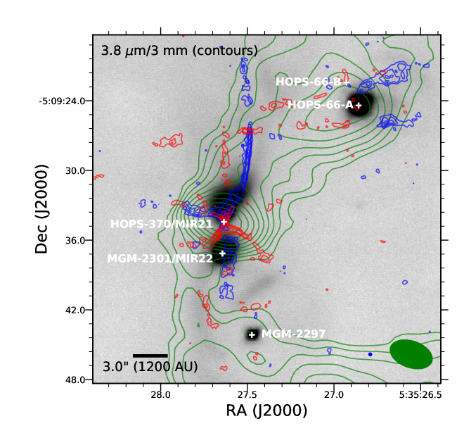
Figure 1: Overview of the HOPS-370/OMC2-FIR3 region. The grayscale image is a 3.8 µm image (L^′-band) from Kounkel et al. (2016), the green contours are ALMA 3 mm combined 12m and ALMA Compact Array data from Kainulainen et al. (2017). The red and blue contours are the low-velocity ¹²CO ($J=3\rightarrow 2$) integrated intensity toward HOPS-370 (blue: -26 to 3 km s^-1, red: 14 to 23 km s^-1) from Tobin et al. (2019) and HOPS-66 (blue: -9 to 7 km s^-1, red: 14 to 28 km s^-1). The positions shown for HOPS-370 and HOPS-66 are from Tobin et al. (2020) and MIR 22/MGM 2301 and MGM 2297 are from Megeath et al. (2012). The ALMA 3 mm contours start at 3$\sigma$ and increase on logarithmically spaced intervals to 100$\sigma$, where $\sigma$=0.0024 mJy beam^-1. The blue contours toward HOPS-370 (HOPS-66) start at 6$\sigma$ (3$\sigma$) and increase on 3$\sigma$ (3$\sigma$) intervals where $\sigma$=0.12 Jy beam^-1 ($\sigma$=0.18 Jy beam^-1). The red contours toward HOPS-370 (HOPS-66) start at 5$\sigma$ (3$\sigma$) and increase on 3$\sigma$ (3$\sigma$) intervals where $\sigma$=0.12 Jy beam^-1 ($\sigma$=0.15 Jy beam^-1). The 3 mm beam is 3.75″$\times$2.27″ and is shown as the green ellipse the lower right corner, while the beam for the ¹²CO moment maps is 0.25″$\times$0.24″ and is the small blue ellipse left of the green ellipse.

We show an overview of HOPS-370/OMC2-FIR3 and its surroundings at 3.8 µm and 3 mm in Figure 1; the 3.8 µm data originally appeared in Kounkel et al. (2016) and the 3 mm data are from Kainulainen et al. (2017). HOPS-370 and HOPS-66 are the protostars present within the 30″ region shown, and two additional sources are also detected: MGM 2297 and MIR 22 (MGM 2301), both of which appear to be more-evolved young stellar objects (YSOs) (Megeath et al., 2012; Nielbock et al., 2003). HOPS-370 was also detected by Nielbock et al. (2003) as MIR 21 in close proximity to MIR 22. Unlike the other sources identified in the image, HOPS-370/MIR 21 does not have a corresponding point source at 3.8 µm due to its deeply embedded nature. The emission north of HOPS-370 is, however, scattered light with its outflow cavities illuminated by the central protostar and disk (e.g., Habel et al. 2020). The ¹²CO ($J=3\rightarrow 2$) integrated intensity maps shown in Figure 1 illustrate the correspondence of the scattered light emission with the low-velocity outflow emission from HOPS-370. HOPS-66 also has some scattered light to the west of its position and ¹²CO emission along its edges.

At first glance it appears that HOPS-370 could be a multiple system given the proximity of the other YSOs detected in the infrared; MIR 22 has a projected separation of just $\sim$3″ ($\sim$1200 au). However, it was argued in Tobin et al. (2019) that MGM 2297 and MIR 22 are likely foreground YSOs and not embedded within an envelope like HOPS-370. The lack of 3 mm emission at their positions is further evidence for lacking an envelope; only HOPS-370 and HOPS-66 have strong 3 mm emission toward their positions. MIR 22 is detected and resolved from HOPS-370 (MIR 21) at 1 to 18 µm, and its SED is consistent with a Class II YSO (Nielbock et al., 2003). Longer-wavelength emission in the mid- to far-infrared is centered on HOPS-370, which is also brighter than MIR 22 beyond 12 µm (Furlan et al., 2014), and MIR 22 is not detected at 870 micron nor at 3 mm (Tobin et al., 2019; Kainulainen et al., 2017). MIR 22 was, however, detected at centimeter wavelengths as a thermal free-free source, $\sim$100$\times$ weaker than HOPS-370/MIR 21 (Osorio et al., 2017). Finally, the ¹²CO maps show no evidence of an outflow associated with MIR 22. Taken together, the evidence indicates that MIR 22 is not likely to be embedded within the envelope of HOPS-370 and is most likely a foreground YSO and not a true companion. Thus, the nearest protostar that is likely to be physically associated with HOPS-370 is HOPS-66 at a projected separation of 6600 au; no additional candidate companions were detected down to 30 au separations (Tobin et al., 2020).

4 Results

The ALMA and VLA observations of HOPS-370 (OMC2-FIR3) offer an unprecedented view of this protostar and its immediate environment in terms of resolution, sensitivity, and breadth of molecular lines/continuum wavelengths observed at $\lesssim$0$\farcs$25 (100 au) resolution. The dust continuum at 0.87 mm and 1.3 mm probes the column density structure toward HOPS-370, and the kinematics are traced by multiple molecular lines that probe complementary physical conditions. The 9 mm continuum on the other hand traces a combination of dust and free-free emission as described in more detail in the following section.

4.1 Continuum Emission

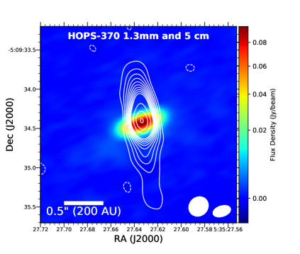
Figure 3: ALMA 1.3 mm continuum images of HOPS-370 with the VLA 5 cm data from Osorio et al. (2017) overlaid showing the relation of the jet traced by 5 cm emission to the disk traced by 1.3 mm emission. The contours start at and increase on $\pm$3$\sigma$ intervals until 30$\sigma$where contours begin to increase on 15$\sigma$ intervals; $\sigma$=7.2 $\mu$Jy. The beam of the 1.3 mm image is 0$\farcs$23$\times$0$\farcs$13 (90 au $\times$51 au) (white ellipse in lower right) and the beam of the 5 cm image is 0$\farcs$26$\times$0$\farcs$23 (101 au $\times$ 90 au) (white ellipse located left of the 1.3 mm beam).

The ALMA and VLA continuum images of HOPS-370 at 0.87 mm, 1.3 mm, and 9 mm are shown in Figure 1. The 0.87 mm and 9 mm images were previously presented in Tobin et al. (2019) and they are reproduced here to emphasize the clear disk emission. The 0.87 mm and 1.3 mm images clearly show the presence of a disk-like structure in the dust continuum emission that we will simply refer to as a disk. This disk is orthogonal to the outflow and jet directions traced both by Herschel (González-García et al., 2016) and the continuum between 5 cm and 9 mm (Osorio et al., 2017). The 5 cm contours from Osorio et al. (2017) are overlaid on the 1.3 mm map in Figure 3, further demonstrating the orthogonal relationship between the disk and the jet.

To measure the geometric parameters of the continuum emission and the integrated flux densities, we fitted Gaussians to the images using the imfit task of CASA 4.7.2. The single-component Gaussians are not perfect fits to the data, but the integrated flux densities agree reasonably well with comparison to the flux density measured within a a polygon surrounding the source.

The results from the Gaussian fits to the continuum emission at 0.87 mm find a deconvolved full width at half maximum (FWHM) of 0$\farcs$34 $\times$ 0$\farcs$11 with a position angle of 109° (Table 2). Adopting the 2$\sigma$ value of the Gaussian fit as the disk radius (Tobin et al., 2020), we find a disk radius of $\sim$113 au, and the inclination of HOPS-370 can be estimated to be $\sim$71° by assuming that it is a geometrically thin disk and then calculating the inverse cosine of the deconvolved minor axis divided by the deconvolved major axis.

The VLA 9 mm continuum image in Figure 1 shows a distinctly different morphology with respect to the ALMA images. Rather than a simple disk feature, the VLA 9 mm image shows a cross-like morphology. The extension in the northeast to southwest direction is longer and more prominent than the extension in the southeast to northwest direction. The longer axis is orthogonal to the major axis of the disk and in the presumed direction of the jet/outflow from HOPS-370. We also show the spectral index map determined from the VLA 9 mm data alone. The spectral index of the emission ($S_{\nu}~{}\propto~{}\nu^{\alpha}$) indicates that the presumed-jet is emitting via the free-free emission process, with values between -0.1 and $\sim$1 (e.g., Anglada et al., 1998). The spectral index in the direction of the disk is close to 2 at the edges of the spectral index map and more consistent with dust emission than free-free emission. Towards the central region, the spectral index is $\sim$1, too low to be dust, and suggesting a significant free-free contribution. Therefore, at 9 mm we trace both the jet and disk emission. The direction of the jet emission at 9 mm is consistent with the resolved jet reported by Osorio et al. (2017) at longer wavelengths (see Figure 3) and the molecular outflow in ¹²CO reported by Tobin et al. (2019).

We fit the VLA data with four Gaussian components simultaneously to describe the cross-like structure observed at 9 mm. The first component is a point-like component to match the peak intensity, the 2nd and 3rd components model the surface brightness distribution of the extended jet, and the 4th component fits the emission along the position angle of the disk. We add parameter estimates to help imfit arrive at a solution that can fit the disk component. The two components are needed for the emission along the jet axis because it cannot be well-described with a single Gaussian. The parameters of each component are given in Table 3; note that the optimization of the 4 components yield one component with a negative flux. When this negative component is combined with the brighter positive component the surface brightness distribution is best reproduced.

The extent of the emission from the disk at 9 mm is estimated to be 0$\farcs$27$\times$0$\farcs$09 and a position angle of 112°, and the flux density of the disk is $\sim$0.73 mJy. The position angle of the disk is consistent with the fit at 0.87 mm, and the angular size at 9 mm is modestly smaller than at 0.87 mm, which is typical when comparing such short and long wavelength data (e.g., Segura-Cox et al., 2016; Tobin et al., 2020).

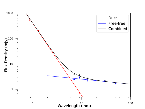
Figure 4: Radio spectrum of HOPS-370. The 0.87 mm, 1.3 mm, and 9.1 mm flux density measurements are from this work; the other measurements are from Osorio et al. (2017) and are listed in Table 2. The red points are assumed to trace only dust emission; a power-law fit is performed finding that the flux density from dust emission scales $\propto$ $\nu^{2.84\pm 0.08}$. The blue points are expected to only trace free-free emission, having their estimated dust emission contribution removed using the power-law fit to the dust emission. A power-law slope is fit to the free-free emission (blue points) finding a dependence $\propto$ $\nu^{0.19\pm 0.08}$. The combined spectrum is drawn as a black line and agrees well with the total flux densities of the points between 7 mm and 20 mm where both emission mechanisms are contributing. The uncertainties on the points at 0.87 mm, 1.3 mm, and 9.1 mm do not include the absolute flux calibration uncertainty of $\sim$10%. The other points from (Osorio et al., 2017) do include the additional absolute flux calibration uncertainty.

We plot the radio spectrum of HOPS-370 in Figure 4, including the flux densities reported in this work and those from Osorio et al. (2017) at longer wavelengths. We fit power-laws to the dust emission between 0.87 mm and 9 mm and remove this estimated contribution from the longer wavelength data points. Then the longer wavelength data points are assumed to only trace the free-free emission from HOPS-370. The flux density of the dust emission scales $\propto$ $\nu^{2.84\pm 0.08}$ and the flux density of the free-free emission scales $\propto$ $\nu^{0.19\pm 0.08}$. The spectral index of the free-free emission indicates partially optically-thick emission since flux density of optically thin free-free emission is expected to scale $\propto$ $\nu^{-0.1}$. This is consistent with the spectral index derived at the position of HOPS-370 by Osorio et al. (2017), while at larger distances from the protostar they found that the jet exhibits non-thermal spectral indices.

4.2 Estimated Disk Mass

The mass of the disk traced by dust continuum emission can be estimated under the assumption of isothermal and optically thin emission using the equation

$$M_{dust}=\frac{D^{2}F_{\nu}}{\kappa_{\nu}B_{\nu}(T_{dust})}.$$ (1)

$D$ is the distance ($\sim$392 pc), $F_{\nu}$ is the observed flux density, $B_{\nu}(T_{dust})$ is the Planck function, $T_{dust}$ is the dust temperature, and $\kappa_{\nu}$ is the dust opacity at the observed wavelength. We adopt $\kappa_{1.3mm}$ = 0.899 cm² g^-1 and $\kappa_{0.87mm}$ = 1.81 cm² g^-1 (Ossenkopf & Henning, 1994), appropriate for protostellar envelopes. We adopt $\kappa_{9.1mm}$ = 0.13 cm² g^-1 by using $\kappa_{1.3mm}$ as a reference point and extrapolating it to 9 mm assuming a dust opacity power-law index of 1.0. This adhoc extrapolation from 1.3 mm to 9 mm is necessary because the Ossenkopf & Henning (1994) models predict an opacity that is too low at 9 mm to yield consistent dust masses with shorter wavelength observations (Tobin et al., 2016a; Segura-Cox et al., 2016; Tychoniec et al., 2018a). $T_{dust}$ is often assumed to be 20 or 30 K (Jørgensen et al., 2009; Tobin et al., 2015; Tychoniec et al., 2018b) for solar-luminosity protostars, consistent with temperature estimates on $\sim$100 au scales (Whitney et al., 2003b). However, as part of the VANDAM Orion survey (Tobin et al., 2020) we used radiative transfer models to estimate the average dust temperature dependence on radius and luminosity. Using those results, we estimate a dust average temperature for a 100 au embedded protostellar disk of $\sim$31 K around a 1 L_☉ protostar. Assuming that T_dust scales as (L/L_☉)^0.25, the expected average temperature for the HOPS-370 disk is $\sim$131 K, with L_bol = 314 L_☉ (Furlan et al., 2016). We finally multiply the resulting value of M_dust by 100, assuming the typical dust to gas mass ratio of 1:100 (Bohlin et al., 1978) to arrive at an estimate of the total disk mass.

The continuum flux density at 1.3 mm is 0.207 Jy, corresponding to a disk mass of 0.084 M_☉. At 0.87 mm, the continuum flux density is 0.533 Jy, corresponding to a disk mass of 0.048 M_☉. Lastly, at 9 mm the continuum flux density from the disk is 0.732 mJy, corresponding to a disk mass of 0.098 M_☉. The modest discrepancy between 0.87 mm and 1.3 mm could result from the dust continuum at 0.87 mm being more opaque and/or uncertainty in the relative dust opacity between 0.87 mm and 1.3 mm. Also, the larger beam at 1.3 mm may enable more emission to be recovered due to more short baselines being included in those observations. The 9 mm measurement agrees well with the others considering the uncertainty in dust opacity and the separation of its emission from the jet using multi-component Gaussian fitting.

4.3 Molecular line Emission

The continuum imaging from both ALMA and the VLA strongly indicate the presence of a disk surrounding HOPS-370. However, the nature of the disk structure can be analyzed further using the kinematics of molecular line emission. To this end, a suite of molecular lines were observed toward HOPS-370 with ALMA at 0.87 mm and 1.3 mm. However, the longer integration of the 1.3 mm data and shorter baseline coverage leads to those data being more sensitive to molecular line emission than the few lines covered in the 0.87 mm observations. The C¹⁸O, ¹³CO, H₂CO, SO, NS, and CH₃OH molecular lines all trace a signature of rotation from the disk revealed by the dust continuum. NS and H¹³CN are the only lines highlighted here from the 0.87 mm observations, but other complex organic molecules are also detected toward the disk at lower S/N (Tobin et al., 2019). Of the other targeted molecular lines, the ¹³CS line was only weakly detected, N₂D⁺ was not detected, and ¹²CO traces the outflow. The non-detection of N₂D⁺ is expected because of the warm temperature of the warm temperature of the disk and inner envelope resulting from the high luminosity of the protostar (e.g., Emprechtinger et al., 2009; Tobin et al., 2013).

We show the integrated intensity maps of the blue- and red-shifted emission of each molecular line (except ¹²CO, N₂D⁺, and ¹³CS) in Figure 5. The integrated intensity maps were created using selected channel ranges where there is spectral line emission using the CASA task immoments. We selected the channels corresponding to blue and redshifted emission using the system velocity of $\sim$11.0 km s^-1 (Tobin et al., 2019); the blueshifted maps are integrated between 4 and 11 km s^-1and the redshifted maps are integrated between 11 and 18 km s^-1. These blue and redshifted integrated intensity images are used to assess the kinematics traced by the particular molecular lines. We do not show the ¹²CO moment maps because they were presented Tobin et al. (2019). We also do not show N₂D⁺ because it is not detected and ¹³CS is not shown because it is only marginally detected.

The consistency of the velocity gradient in all well-detected molecular lines indicates that the disk around HOPS-370 is clearly rotating and may be rotationally supported. We note that the peaks of the line emission can be northeast and/or southwest with respect to the center of the continuum position, and these peaks tend to avoid the midplane traced in dust continuum. Continuum opacity and/or line opacity are likely to cause this feature; molecular freeze-out is not likely because of the warm disk temperatures due to the high luminosity of the protostar.

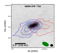
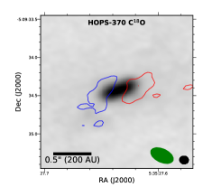
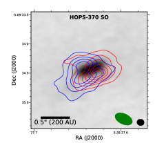
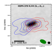
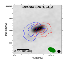
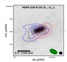
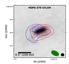
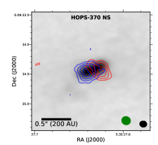
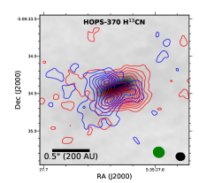
Figure 6: Position-velocity (PV) diagrams of the molecular line emission taken across the major axis of the disk, summed within a 0$\farcs$6 strip. The rotation signature of the disk is evident on scales less than $\pm$1″ at blue- and red-shifted velocities. The emission on scales $>$1″ between velocities of $\sim$9.5 and 13 km s^-1 corresponds to emission from the cloud/envelope that is not well-recovered in these observations. The C¹⁸O emission, however, is dominated by an extended, low-velocity component and the higher-velocity disk emission is only marginally-detected. The white dashed line shows the source velocity at $\sim$11 km s^-1, and the white dotted line is the Keplerian velocity curve for a 2.5 M_☉ protostar drawn for comparison. The contours drawn start at and increase on 5$\sigma$ intervals, where $\sigma$ is $\sim$4$\times$ the image RMS from Table 1.

The integrated intensity maps only show limited spectral information; therefore we also show position-velocity (PV) diagrams for each molecular line in Figure 6. The PV diagrams were extracted from the molecular line data cubes using a custom Python code to obtain a complementary view of the kinematic structure. The PV diagrams are extracted along a 0$\farcs$6 wide strip (15 pixels) along the major axis of the disk, at a position angle 100° East of North. The emission is summed within the 0$\farcs$6 strip to produce a two dimensional spectrum. The PV diagrams bear strong resemblance to other protostellar disks that have been detected and characterized (Tobin et al., 2012; Sakai et al., 2014; Oya et al., 2015; Aso et al., 2017). The PV diagrams bear the signature of a rotating Keplerian disk with a finite radius: a linear velocity gradient transitioning from blue to red-shifted on opposite sides of the protostar and higher-velocity emission from spatial scales closer to the central protostar following a Keplerian velocity profile.

These features are produced because the outer radius of the disk causes the emission from the largest radii of the disk to have a similar velocity profile to a rotating ring; in this case the ring is the outer disk. The finite radius of the outer disk means that Keplerian rotation will not continue to spatial scales that extend beyond the disk. Then radii closer to the protostar rotate more quickly, producing the higher-velocity emission that is typically associated with Keplerian rotation toward embedded protostars. The linear transition from blue to red is most easily seen in the PV diagrams for NS and SO molecules. However, the transition is not always easily detectable toward protostellar disks (e.g., Tobin et al., 2012; Ohashi et al., 2014; Murillo & Lai, 2013) due to spatial filtering and blending with the infalling envelope and the molecular cloud near the system velocity. But, certain molecular transitions that specifically trace the disk and not the surrounding cloud/envelope show the low-velocity emission of the disk with higher fidelity. This is due to a variety of possible reasons, but mainly critical density, chemistry, excitation temperature. The lines SO, CH₃OH, NS, and H₂CO ($J=3_{2,2}\rightarrow 2_{2,1}$), ($J=3_{2,1}\rightarrow 2_{2,0}$) with T_ex $\sim$60 K best trace the disk of HOPS-370.

Previous studies have been able to use point-like line emission in velocity channels away from the system velocity toward disks around lower-mass Class 0 and Class I protostars to fit the emission centroids from PV diagrams, data cubes, and/or the uv-data themselves to map the rotation curves in one dimension. In these cases, the emission centroids systematically changed with each velocity channel, high velocities near the continuum source and lower velocities centered farther from the continuum source (Yen et al., 2013; Tobin et al., 2012; Ohashi et al., 2014). However, the clear non-Gaussian emission in the images prevents such analyses from being viable for HOPS-370. Thus, the rotation curve must be examined using modeling of the molecular line emission which will be discussed in Section 5.

4.4 Near Infrared Spectrum

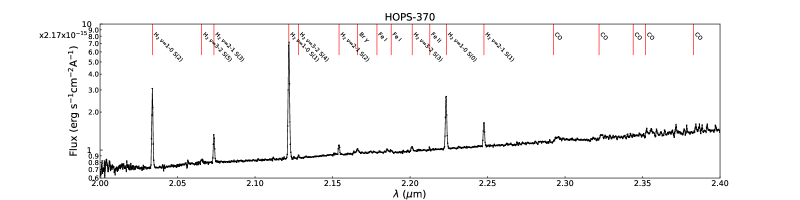
Figure 7: Near-infrared spectrum of HOPS-370 from 2 to 2.4 µm. The prominent spectral features are molecular hydrogen emission lines that are presumably due to shock-heated H₂ in the outflow from HOPS-370. Emission in Br $\gamma$ and CO band heads are also well-detected, though less prominent. Absorption lines are absent in the spectrum of HOPS-370, indicating that the spectrum is highly veiled.

The near-infrared spectrum of HOPS-370 is shown in Figure 7 from 2 to 2.4 µm. HOPS-370 is also detected shortward of 2 µm  but with lower S/N and is not shown. The main spectral features are the prominent H₂ emission lines detected throughout the band. We also detect weaker emission from the Brackett $\gamma$ (Br $\gamma$) atomic hydrogen recombination line and CO band head emission. Continuum emission is detected, but there are no obvious photospheric absorption features detected in this medium resolution spectrum. The H₂ emission lines are likely associated with shocks in the outflow from HOPS-370 given that most of the near-infrared emission detected in this spectrum is from the outflow cavity due to the central protostar being too highly extincted. The properties of the Br $\gamma$ emission are of the greatest interest to extract due to their frequent association with accretion processes in young stars (e.g., Muzerolle et al., 1998; Connelley et al., 2009). The equivalent width of the Br $\gamma$ line is -1.42 Å, with an integrated flux of 2.9$\times$10^-15 erg s^-1 cm^-2. This line flux translates to a Br $\gamma$ luminosity of 5.6$\times$10²⁸ erg s^-1 or 1.5$\times$10^-5 L_☉. The equivalent width and line luminosity of the Br $\gamma$ line are within the ranges typically observed toward Class I protostars by Connelley & Greene (2010). However, these values are on the low end for a protostar that is expected to be accreting rapidly. The interpretation of the line emission will be further discussed in Section 6.3.

5 Radiative Transfer Modeling

In order to further interpret our dust continuum and molecular line observations, radiative transfer modeling is necessary. We use molecular line radiative transfer modeling to fit the kinematics of the system, primarily constraining the protostar mass and rotating disk radius. The continuum radiative transfer modeling on the other hand enables more detailed constraints on the disk structure to be derived. We make use of the software packages pdspy (Sheehan & Eisner, 2017; Sheehan et al., 2019) and RADMC-3D (Dullemond et al., 2012) for our modeling efforts.

5.1 Molecular Line Modeling

The molecular line images and PV diagrams show strong rotation signatures (Figures 5 and 6). To quantitatively determine if the rotation is tracing a Keplerian disk and, if so, to measure the protostar mass we must make use of radiative transfer modeling to fully utilize the constraints offered by the channel maps for multiple molecular lines. The pdspy package has distinct modes for fitting molecular line kinematic data and continuum data. The basis for both models is an analytic physical model for a protostellar system with a surrounding disk embedded within an infalling envelope.

5.1.1 Physical Model

The disk structure for the molecular line models uses an exponentially-tapered disk density profile (Lynden-Bell & Pringle, 1974). The exponentially-tapered density profile is described by

$$\Sigma(r)=\,\Sigma_{0}\left(\frac{r}{r_{c}}\right)^{-\gamma}\,\exp\left[-\left(\frac{r}{r_{c}}\right)^{(2-\gamma)}\right],$$ (2)

where $r$ is the disk radius defined in cylindrical coordinates. The power-law index of the surface density profile is defined by $\gamma$. The normalization constant, $\Sigma_{0}$ is given by

$$\Sigma_{0}=\frac{(2-\gamma)M_{d}}{2\pi r_{c}^{2}},$$ (3)

where $M_{d}$ is the disk mass and the other parameters are as defined above. The vertical structure of the disk is set by hydrostatic equilibrium, assuming that the disk is vertically isothermal such that

$$h(r)=\left(\frac{k_{b}\,r^{3}\,T_{g}(r)}{G\,M_{*}\,\mu_{m}\,m_{H}}\right)^{1/2},$$ (4)

where $k_{b}$ is the Boltzmann constant, $G$ is the gravitation constant, $M_{*}$ is the central stellar mass, $\mu_{m}$ is the mean molecular weight of 2.37 (Lodders, 2003), $m_{H}$ is the mass of a hydrogen atom, and $T_{g}(r)$ is the temperature profile defined as

$$T_{g}(r)=T_{0}\,\left(\frac{r}{1\,\mathrm{au}}\right)^{-q}$$ (5)

where both $T_{0}$ and $q$ can be free-parameters.

The rotating, infalling envelope is described by the density profile of a rotating collapse model (Ulrich, 1976; Cassen & Moosman, 1981; Terebey et al., 1984). The envelope density profile is defined as

$$\footnotesize\rho=\frac{\dot{M_{env}}}{4\pi}\left(GM_{*}r^{3}\right)^{-\frac{1}{2}}\left(1+\frac{\mu}{\mu_{0}}\right)^{-\frac{1}{2}}\left(\frac{\mu}{\mu_{0}}+2\mu_{0}^{2}\frac{R_{c}}{r}\right)^{-1}$$ (6)

where $\dot{M}_{env}$ is the mass infall rate of the envelope onto the disk, $R_{c}$ is the centrifugal radius where the infalling material has enough angular momentum to orbit the star, $\mu$ = cos $\theta$, and $\mu_{0}$ is the cosine polar angle of a streamline out to r $\rightarrow$ $\infty$. The density profile inside of $R_{c}$ will be $\rho_{env}\propto r^{-1/2}$, and outside $R_{c}$, it will be $\rho_{env}\propto r^{-3/2}$. For the sake of our modeling, we consider $R_{c}$ to be equivalent to the outer disk radius for a truncated disk model and the critical radius for an exponentially-tapered disk. Thus, $R_{c}$ = $r_{c}$ from Equations 2, 3, and 4.

The envelope model includes outflow cavities with reduced envelope density. The width of the outflow cavities are parameterized as

$$z~{}>~{}1~{}au+r^{\xi},$$ (7)

and the envelope density is reduced by a factor of $f_{cav}$. The outflow cavity opening angle will be less than 45° for $\xi$ $<$ 1 and greater than 45° for $\xi$ $>$ 1. The outflow cavity opening angle, $\psi$, can be directly calculated from

$$\psi=2tan^{-1}(\xi).$$ (8)

The velocity profile of the infalling envelope is also adopted from the rotating collapse model (Ulrich, 1976) where

$$\scriptsize v_{r}(r,\theta)=-\left(\frac{GM_{*}}{r}\right)^{1/2}\,\left(1+\frac{\cos\theta}{\cos\theta_{0}}\right)^{1/2},$$ (9)

$$\scriptsize v_{\theta}(r,\theta)=-\left(\frac{GM_{*}}{r}\right)^{1/2}\,(\cos\theta_{0}-\cos\theta)\,\left(\frac{\cos\theta_{0}+\cos\theta}{\cos\theta_{0}\sin^{2}\theta}\right)^{1/2},$$ (10)

$$\scriptsize v_{\phi}(r,\theta)=-\left(\frac{GM_{*}}{r}\right)^{1/2}\,\left(\frac{\sin\theta_{0}}{\sin\theta}\right)\,\left(1-\frac{\cos\theta}{\cos\theta_{0}}\right)^{1/2}.$$ (11)

The velocity profile of this equation results in rotational velocity in the equatorial plane of the envelope that is equivalent to the Keplerian orbital velocity at a radius of $R_{c}$. As such, material located within the disk at radii smaller than $R_{c}$, have velocities described by Keplerian rotation with

$$v_{\phi}(r)=\left(\frac{GM_{*}}{r}\right)^{1/2}.$$ (12)

The $v_{r}$ and $v_{\theta}$ components are expected to cancel out upon incorporation into the disk.

5.1.2 Parameters

We are principally interested in fitting the protostar mass and disk radius with the molecular line models. However, we also fit disk mass, the system velocity, position angle, central position, power law index of the surface density profile $\gamma$, and temperature at 1 au. In addition to these parameters, we computed a second set of models that also fit the envelope mass and radius that are presented in the Appendix. We do not regard $\gamma$ with high confidence given that it may not truly reflect the underlying surface density profile, rather a convolution of the radial abundance profile, surface density profile, and dust continuum opacity. Furthermore, the envelope mass and radius will also not be robust because we do not include uv-data from scales $<$50 k$\lambda$ (4″) in our fitting, and the extended emission from the envelope is weak for the molecular lines shown in Figures 5 and 6. Also, we do not account for a radial variation in the abundance profile of molecules in our modeling. Moreover, the disk and envelope masses are degenerate with the assumed molecular abundances (which are uncertain). The full range of parameters fixed and varied in the line modeling are provided in Table 4.

To limit the parameter space, we fix several parameters that do not strongly impact the modeling results or have constraints from other data. The inclination is fixed at 72.2°, as determined from an earlier model fit to the continuum data (Section 5.2); the small ($\sim$2°) difference has an insignificant effect on the fit. Finally, we fix the power-law index of the temperature profile, $q$, to be 0.35, appropriate for protostellar disks (van ’t Hoff et al., 2018). We adopt gas phase abundances as follows: H₂CO abundance of 1.0$\times$10^-9 per H₂, SO abundance of 3.14$\times$10^-9, CH₃OH abundance of 1.0$\times$10^-8, and NS abundance of 3.14$\times$10^-9. The CH₃OH abundance is adopted from the estimate made toward HOPS-370 and HOPS-108 in Tobin et al. (2019), while the SO and H₂CO abundances are adopted to be consistent with the range of abundances reported in Schöier et al. (2002); Gerner et al. (2014); Feng et al. (2016), and the NS abundance is within the ranges found by Crockett et al. (2014) and Xu & Wang (2013). When two different molecules are modeled simultaneously, the abundance of one molecule is allow to vary such that a single disk mass can fit the data well.

5.1.3 Model Fitting

To fit models with the underlying physical structure described in the previous section, we employ a Markov-Chain Monte Carlo (MCMC) modeling framework to sample the parameter space and fit radiative transfer models. We use the software package pdspy (Sheehan & Eisner, 2017; Sheehan et al., 2019), which uses emcee (Foreman-Mackey et al., 2013) to conduct the MCMC and sample the parameter space, RADMC-3D (Dullemond et al., 2012) is used to compute the molecular line radiative transfer in the limit of local thermodynamic equilibrium (LTE) for each sample of the parameter space, and finally the GPU Accelerated Library for Analysing Radio Interferometer Observations (GALARIO; Tazzari et al., 2018) is used to Fourier transform the synthetic datacubes output by RADMC-3D for comparison with the visibility data. Our molecular line modeling is based on the implementation presented in Sheehan et al. (2019) to fit the protostar mass and disk radius. We restrict fitting to uv-data at baselines longer than 50 k$\lambda$ to limit the contribution of emission more extended than 4″, which is not recovered in our observations.

We calculate the goodness of fit for each model using the visibility data from the observations and model at each velocity channel between 0 and 19.8 km s^-1 with 0.33 km s^-1 channels. The MCMC uses 200 walkers to explore the multi-dimensional parameter space. During a single iteration, all walkers are advanced by running a model and the goodness of fit is calculated for each model. After the completion of a single iteration, each walker takes its next step by comparing its likelihood with the likelihood of the other walkers, and moving towards or away from them based on the comparison.

We used the model to fit the molecular line emission, in the uv-plane, toward HOPS-370 that best traces the disk without significant contamination from the molecular cloud/envelope. Thus, the molecular lines fit are SO, CH₃OH, NS, and H₂CO ($J=3_{0,3}\rightarrow 2_{0,2}$), ($J=3_{2,2}\rightarrow 2_{2,1}$), and ($J=3_{2,1}\rightarrow 2_{2,0}$). We excluded ¹³CO and C¹⁸O from the fitting due to their low S/N. The modeling includes the dust continuum emission produced by the disk parameters of a particular model run during the course of the MCMC fitting. The continuum emission is generated using dust grains with $a_{min}$=0.005 µm, $a_{max}$=1 µm and $p$=3.5 with optical properties from Pollack et al. (1994); this dust grain size distribution and composition reproduces the features of a typical protostellar SED well (Sheehan & Eisner, 2014, 2017) and provides opacities as a function of wavelength similar to Ossenkopf & Henning (1994). The continuum emission is included in the radiative transfer calculation to approximate an attenuation of the line emission by the continuum opacity. Then, the continuum is subtracted from the model to to approximate the continuum subtraction that has been applied to the observed data. Note that the continuum emission that is calculated and subtracted corresponds to the continuum from the molecular line model setup and not from the fit to the dust continuum data described in Section 5.2.

In addition to fitting individual spectral lines, we also performed simultaneous fits to those species that had multiple transitions. The capability exists in pdspy to fit both two species simultaneously and multiple transitions of the same molecular species. We computed the following simultaneous fits: all three observed H₂CO lines, only the H₂CO ($J=3_{2,2}\rightarrow 2_{2,1}$) and ($J=3_{2,1}\rightarrow 2_{2,0}$) lines, SO and H₂CO, SO and CH₃OH, SO and NS, NS and CH₃OH, and NS and H₂CO. In the case of fitting two different molecules, we allowed the abundance of one molecule to vary in order to enable fitting to converge with a single disk mass.

5.1.4 Modeling Results

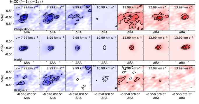
Figure 8: Comparison of molecular line data to the kinematic model fits. The top row shows the data, the middle row shows the model, and the bottom row shows the residuals. We show H₂CO ($J=3_{0,3}\rightarrow 2_{0,2}$) in Figure 7a, H₂CO ($J=3_{2,2}\rightarrow 2_{2,1}$) in Figure 7b, H₂CO ($J=3_{2,1}\rightarrow 2_{2,0}$) in Figure 7c, and SO ($J_{N}=6_{5}\rightarrow 5_{4}$) in Figure 7d, CH₃OH in Figure 7e, and NS in Figure 7f; the RMS noise in each panel is 0.017, 0.013, 0.013, 0.016, 0.011 and, 0.021 mJy beam^-1, respectively. The contours in all panels start at and increase on 3$\sigma$ intervals, using the same measurement of the RMS noise for the data, model, and residual. The color stretch is also identical for the data, model, and residual for each molecule.

We present the results from the model fitting without including the envelope in Figure 8. The disk-only models find similar protostar mass and disk radii as the models that include an envelope; the model results that include an envelope are presented in the Appendix. Figure 8 shows the results from fitting three H₂CO lines and the SO line; we also show the results from CH₃OH and NS when simultaneously fit with H₂CO. The fit parameters for each line or combination of lines are given in Table 5. The best fitting values are determined from the median of the posterior distribution for each parameter and the uncertainties reflect the standard deviation of the posterior distribution. In calculating the best fitting values and their uncertainties, we filtered outliers from the posterior distributions by rejecting walkers that did not conform to a $\xi^{2}$ distribution. These outliers were typically walkers that never converged to the best fitting values and typically represent less than 5% of the 200 walkers used. To avoid filtering too aggressively, we relaxed the filtering criteria such that we included at least 95% of the walkers in the final statistics.

As can be seen in Table 5, there is variation in the best fitting protostar mass and disk radius, depending on the molecule(s) being fit. We note that the uncertainties listed in Table 5 are smaller than the differences between best-fit values for the different molecules fit; 1$\sigma$ uncertainties are shown, but differences are even in excess of 3$\sigma$ uncertainties. The variation of best fit parameters can reflect both the adopted model not being fully representative of the prototstellar disk and envelope, as well as the molecular line emission from the various molecules tracing different spatial extents. Differences in the spatial distribution of molecular line emission have been found toward several protostars on comparable spatial scales (Sakai et al., 2014; Yen et al., 2014). The models assume a constant molecular abundance with radius and if this is not true, systematic differences between modeling of different molecules can arise.

Averaging the 12 independent fits we find an average protostar mass of 2.5$\pm$0.15 M_☉. The full range of best fitting protostar masses is between 1.8 and 3.6 M_☉, with the two highest and lowest masses being quite different from the other 10 fits, which are much closer to the average value. The best fitting disk radii are between 70 and 121 au. Averaging the 12 independent fits we find an average radius of $\sim$94$\pm$13 au. The uncertainties of the average are calculated using the median absolute deviation (MAD) from the collection of 12 model fits, scaled such that the MAD would correspond to one standard deviation of a Normal distribution. Other average fitting parameters are V_lsr = 11.1$\pm$0.04 km s^-1, PA = 352.7$\pm$1.4°, $\gamma$ = 0.92$\pm$0.14, and the position offsets are also very small, typically $\sim$0$\farcs$01. We discuss the other fitted parameters and the possible ramifications of various assumptions for the modeling in the Appendix.

We compare our best fitting protostar mass of $\sim$2.5 M_☉ to the PV diagrams in Figure 6. We overlaid a Keplerian rotation curve for a mass of 2.5 M_☉ at an inclination of 72.2°(see Section 5.2). The Keplerian rotation curves encompass the high-velocity emission, indicating that the average fitted mass of 2.5 M_☉ is quite consistent with the observed data. Thus, the measured protostar mass clearly confirms that HOPS-370 is an intermediate-mass protostar.

5.2 Dust Continuum Modeling

To determine the physical structure of the disk around HOPS-370, the dust continuum emission must also be modeled using radiative transfer, but using a more realistic treatment of the disk and envelope temperature structure than the molecular line modeling employed. We model the disk and envelope around HOPS-370, also with pdspy and RADMC-3D, but taking advantage of the radiative equilibrium mode where the photons are propagated from a central luminosity source and the temperature structure of the disk and envelope are calculated self-consistently. This mode is much more computationally intensive that using prescribed temperature profiles, as such we could not make use of this mode for the molecular line modeling. We follow the methodology employed by Sheehan & Eisner (2017), which utilizes the pdspy package, employing the same underlying MCMC sampling of the parameter space as the molecular line fitting, using 200 walkers.

The dust continuum and SED modeling within pdspy adopts the same envelope physical model as the molecular line modeling. The principal differences, however, are in the temperature and density structure of the disk. The volume density structure of the disk is defined as

$$\rho(r)=\left(\frac{r}{r_{c}}\right)^{-\alpha}\frac{\Sigma(r)}{\sqrt{2\pi}\ h(r)}\,\exp\left(-\frac{1}{2}\left[\frac{z}{h(r)}\right]^{2}\right),$$ (13)

where $\Sigma(r)$ is defined in Equation 3, $\alpha$ is the power-law index of the disk volume density profile, $z$ is the height above the disk midplane in cylindrical coordinates, and $h(r)$. The vertical density structure for the disk in the continuum model is not defined by hydrostatic equilibrium, but parameterized as

$$h(r)=h_{0}\left(\frac{r}{1\text{AU}}\right)^{\beta}.$$ (14)

Here $\beta$ refers to the power-law index that defines how the vertical scale height of the disk varies with radius in the disk, not the power law index of the dust opacity curve. The power-law index of the disk surface density profile is equivalent to $\gamma$ = $\alpha$ - $\beta$, resulting from the multiplication of the volume density profile and the vertical density profile. The temperature structure for the continuum model is not prescribed as it is for the molecular line model. The temperature of the dust is set by the radiative equilibrium calculation performed by the RADMC-3D code. The disk dust properties are taken from Woitke et al. (2016) where the maximum size of the dust grains is parameterized as $a_{max}$ and the power-law index of the dust grain size distribution, $p$, ($n(a)~{}\propto~{}n^{-p}$), both of which are free parameters; $a_{min}$ is fixed to be 0.05 µm. The envelope dust properties are taken from Pollack et al. (1994) with $a_{min}$=0.005 µm, $a_{max}$=1 µm and $p$=3.5.

We simultaneously fit the 0.87 mm continuum emission in the uv-plane and the SED from the near-infrared to the millimeter. The parameter space explored for the dust continuum is significantly larger than that of the molecular line kinematic modeling because now we fit the emission of the envelope, disk, and the overall SED of the system. Our goodness of fit metric is a weighted $\chi$² where

$$\chi^{2}=\omega_{0.87mm,vis}\chi_{0.87mm,vis}^{2}+\omega_{SED}\chi_{vis}^{2}.$$ (15)

The terms $\omega_{0.87mm,vis}$ and $\omega_{SED}$ are determined empirically to be 0.2 and 1.0. The $\chi$_vis are calculated by directly comparing the real and imaginary visibility components between the data and the model; the comparison is done with the two dimensional visibility data and not using azimuthally averaged one dimensional profiles, such profiles are only used for visual comparison of the models and data.

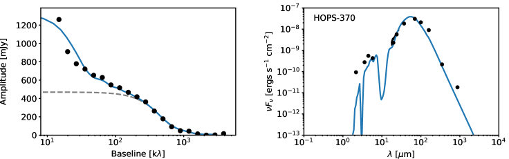
Figure 14: Model fit visibilities and SED of HOPS-370. The circularly averaged visibility amplitudes at 0.87 mm is shown in the left panel and the SED is shown in the right panel. Note that the model fitting was performed using the two dimensional visibility data and not the azimuthally-averaged plots shown here. In all panels, the black points show the data and the model fit is shown as the thick blue line; statistical uncertainties are smaller than the points shown. The left panel also shows the contribution to the visibility amplitudes from only the protostellar disk (gray dashed line), while the thick blue line shows the total contribution from both the disk and envelope to the visibility amplitudes. The SED includes photometry from Spitzer, Herschel, APEX (350 and 870 µm) from Furlan et al. (2016), 19 and 37 µm flux densities from SOFIA (Adams et al., 2012), and the SOFIA FORCAST spectrum (Karnath et al. in prep.).

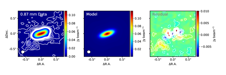
Figure 15: Image comparison of the model fits to HOPS-370. The data are shown in the left panel, the model is shown in the middle panel, and the residuals are shown in the right panel. The residual image is generated from imaging the residual visibility amplitudes and does not reflect an image-plane subtraction. The contours in the data and residual image start at and increase on $\pm$3$\sigma$ intervals; negative residuals are plotted as dashed contours, $\sigma$=0.31 mJy beam^-1. The contours are shown on the data to highlight the emission that is not shown due to the color scaling.

The best-fitting models compared to the data are shown in Figures 14 and 15. The circularly averaged visibility amplitude profile at 0.87 mm demonstrates that the model fits the 0.87 mm visibility data quite well at uv-distances greater than $\sim$50 $k\lambda$. Also plotted in Figure 14 is the estimated contribution of just the disk alone to the visibility amplitude profile, this shows that the envelope contributes significantly to the emission at uv-distances less than 300 k$\lambda$. The fit to the SED, also shown in Figure 14, is not perfect, but is a close approximation to the the shape and flux densities of the SED. Some flux density points are over or under predicted, but the relatively low angular resolution of Spitzer and Herschel at wavelengths longer than 10 µm makes it difficult to construct a SED that only includes emission from HOPS-370. However, the fact that it is the most luminous protostar within an arcminute means that contributions from other sources will not have an extremely negative impact on the SED. But, extended emission at wavelengths longer than 100 µmcan cause the luminosity to be over estimated at those wavelengths.

We show an image-plane comparison of the data, model, and residuals in Figure 15. The residual images are generated from the residual visibility amplitudes and not an image-plane subtraction. The main disk feature in the continuum is well-modeled and removed from the residual image, but the 0.87 mm residual image does show structure around the protostar that is not captured in the model. There are clear over-subtractions in the outer disk and center, while there are under-subtractions within the disk as well. This residual emission may represent complexities in the disk and inner envelope density structure that are not reflected in our physical model. We note that in the 0.87 mm residual map there is compact emission southeast of the protostar (-0$\farcs$4, -0$\farcs$3), but its nature is unclear and could stem from heating along the outflow cavity wall.

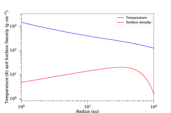
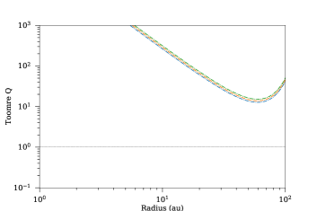
Figure 16: The left panel shows the radial temperature and surface density profiles of the disk of HOPS-370, derived from the best fitting radiative transfer model. The right panel shows the inferred Toomre Q parameter calculated using Equation 19. The three lines correspond to three different assumptions of protostar mass: 2.1, 2.5, and 2.7 M_☉ in order from the lowest to highest lines. These results indicate that gravitational instability is not significant within the disk of HOPS-370.

We list the parameters and their best fitting values for the disk of HOPS-370 in Table 6, but discuss the most relevant parameters here, which are the disk radius, disk mass, surface density power-law index, and luminosity. The best fitting disk mass is 0.035 M_☉, which is somewhat lower than the mass calculated under the assumption of optically thin emission and an average temperature of 131 K. However, the maximum dust grain size fit by the modeling is 440 µm, so the dust of the model will emit much more efficiently at 0.87 mm due to its opacity than the Ossenkopf & Henning (1994) dust adopted for the simple mass estimate. We do note that the temperature of the disk in the model fit at a radius of 100 au is $\sim$122 K (Figure 16), which implies that the disk average temperature is comparable to the value estimated from the bolometric luminosity. The luminosity of the protostar is fit to be 276 L_☉, which is a bit less than L_bol of 314 L_☉. The more extended emission at wavelengths longer than 100 µm, which is not fit well by the model SED, could result from warm dust surrounding the protostar and may cause the bolometric luminosity to be over-estimated.

The best fitting envelope mass is 0.12 M_☉ with a radius of $\sim$1900 AU. However, the poor sampling of short uv-distances will limit the robustness of the envelope model fit to the ALMA visibility data, despite the additional constraints from the SED. This is because the SED shortward of 100 µm is most sensitive to the inner envelope density and not the overall mass or radius. The overall mass and radius can affect the longer wavelength data more, but there is a degeneracy between dust temperature and mass. Thus, it is possible that the total mass and radius of the envelope is not accounted for in our model fit. The full outflow cavity opening angle is fit to be $\sim$98°, as computed from the value of $\xi$ in Table 6. While this may seem large at first glance, it appears comparable to the width of the outflow cavities near the protostar viewed in low-velocity ¹²CO emission and shown in Tobin et al. (2019). However, the shape of the full outflow cavity extent may be more parabolic, meaning that the apparent opening angle at larger radii will appear smaller.

The disk radius from the continuum fit, 62.1 au, is smaller than our estimate of the radius from Gaussian fitting; however, Figure 16 does show that the fitted disk surface density is $\sim$1.3 g cm^-2 at 100 au because the exponentially-tapered disk extends beyond the critical radius $r_{c}$. The continuum disk radius is also comparable to the range of exponentially-tapered disk radii fit with the molecular line modeling. However, it is known that the gas disk tends to be larger than the dust disk from Class II disks (Ansdell et al., 2018). This is thought to be caused by radial drift of dust particles due to gas drag experienced because the gas orbits the star at slightly sub-Keplerian velocities (Weidenschilling, 1977). Thus, the dust in protostellar disks may also experience radial drift (Birnstiel et al., 2010), which would cause a disagreement between the dust and gas disk radii.

While the disk outer radius is reasonable, there are some peculiarities with the disk structure. The surface density profile increases with radius as $\Sigma$ $\propto$ $r^{0.47}$. However, this may result from the high opacity of the disk and its high inclination, leading to a sub-optimal model fit. Moreover, given that the steepness of the exponential cutoff depends on $\gamma$, the smaller $\gamma$ leads to the disk surface density to fall off more quickly. Thus, the best fitting $\gamma$ may tell us more about the sharpness of the disk’s ‘edge’ than the surface density profile. The negative residuals from over-subtraction in Figure 14 could indicate that the disk needs a sharper cutoff than the exponential taper provides. In addition to $\Sigma$ increasing with radius, the inner disk radius is fit to be 0.51 au. This radius slightly smaller than the radius at which dust is expected to be destroyed, where T$\sim$1400 K which occurs at $\sim$1 au in our model.

The disk vertical height is also not highly flared, the best fitting in disk scale height with radius is $h(r)$ $\propto$ $r^{0.66}$, normalized to 0.131 au at 1 au, which indicates that the disk height increases slowly with radius. This fit likely reflects the large grain population of the disk and may not accurately reflect the disk properties of the smaller grains and/or gas disk.

6 Discussion

The ALMA and VLA continuum and molecular line emission are reshaping our understanding of HOPS-370/OMC2-FIR3 by providing a detailed view of the disk and jet toward this candidate intermediate-mass protostar. While the T_bol of 71 K measured from the SED suggests that this is a Class I protostar (Furlan et al., 2016), its location near the canonical border of 70 K between Class 0 and I indicates that HOPS-370 is very much a young, embedded protostar.

The continuum images indicate that there are no resolved companions within 1000 AU, and the nearby infrared sources mentioned in Section 3 do not appear to be embedded within the envelope of HOPS-370. Thus, HOPS-370 may have been the result of a single core collapsing within the OMC2 region, and its seemingly well-ordered disk and outflow morphology makes it an ideal system for characterizing the early evolution of an intermediate-mass protostar.

HOPS-370 also appears to have a profound influence on the environment of the surrounding protostars. For instance, there is strong evidence that its outflow is interacting with the ambient cloud and the OMC2-FIR4 clump, which is associated with HOPS-108 and at least six other protostars (Shimajiri et al., 2008; López-Sepulcre et al., 2013; Furlan et al., 2014; González-García et al., 2016; Osorio et al., 2017; Tobin et al., 2019). The shocks associated with the interaction are strong enough to emit non-thermal synchrotron emission (Osorio et al., 2017), and it is the brightest known far-infrared line emitter in Orion outside of the Orion Nebula itself (Manoj et al., 2013).

The dust continuum emission toward HOPS-370 indicates a large disk around the protostar. The inferred disk radius from a Gaussian fit to the dust continuum of 113 au is in excess of the disk radii around most Class 0 and I protostars (Harsono et al., 2014; Yen et al., 2017; Tobin et al., 2020). Even if one only considers the 62 au radius from modeling, it is still larger than the mean disk radii for protostars in Orion; the mean disk radii for Class 0 and I protostars in Orion are $\sim$45 au and $\sim$37 au, respectively (Tobin et al., 2020). However, it is not clear if intermediate-mass protostars typically have larger disks given that Tobin et al. (2020) observed no correlation between disk radius and bolometric luminosity.

6.1 Protostellar Mass and Accretion Rate

Stellar mass is the most fundamental property of a stellar system, given that the entire evolution of a star is determined by its mass. Thus, the protostar mass measurement of $\sim$2.5 M_☉ for HOPS-370 solidifies its status as an intermediate-mass protostar still in the early stages of formation. While there is some uncertainty in the mass when fitting the molecular line emission for kinematics of different molecules, the differences are most likely systematic because SO, CH₃OH, NS, and H₂CO do not trace the same material in the disk and inner envelope, meaning that their abundance profiles in the radial and vertical directions are not equivalent.

We can see this particularly in the SO and NS line emission, which are more compact than the H₂CO ($J=3_{0,3}\rightarrow 2_{0,2}$) line emission (Figures 5 and 6), with H₂CO ($J=3_{0,3}\rightarrow 2_{0,2}$) emission extending to slightly higher velocities on the blue-shifted side. The masses from fitting are between 1.8 to 3.6 M_☉; however, considering the full range of masses fit the mean is $\sim$2.5 M_☉ with a fractional uncertainty of $\sim$7%.

To determine the mass accretion rate, we use the equation for accretion luminosity

$$L_{acc}~{}=~{}\frac{GM_{ps}\dot{M}}{R_{ps}},$$ (16)

where $G$ is the gravitational constant, $M_{ps}$ is the protostar mass, $\dot{M}$ is the mass accretion rate from the disk to the protostar, and $R_{ps}$ is the protostar radius. Thus, $M_{ps}$ is now the most highly constrained of the parameters needed to determine $\dot{M}$. Palla & Stahler (1993) calculated pre-main sequence evolution of intermediate-mass stars, indicating that the luminosity of the protostellar object itself ($L_{*}$) will be less than $\sim$10 L_☉  meaning that the vast majority of the L_bol = 314 L_☉ will be dominated by luminosity from mass accretion. We assume simplistically that

$$L_{acc}~{}\approx~{}L_{tot}-L_{*}.$$ (17)

Palla & Stahler (1993) also calculated that the likely stellar radius for a protostar like HOPS-370 is $\sim$5 R_⊙. We note that these protostellar stellar birthline models require assumptions that are still subject to debate, the effect of accretion in particular, so there is uncertainty in the most appropriate stellar radius to assume for a given mass (Baraffe et al., 2009; Hosokawa et al., 2010).

If assume L_bol $\approx$ $L_{tot}$, then the mass accretion rate from the disk to the protostar is likely 2.25$\times$10^-5 M_☉ yr^-1. This value compares well to the outflow rate of $\sim$2.3$\times$10^-6 M_☉ yr^-1 calculated from the [OI] jet emission by González-García et al. (2016) if one assumes that the outflow rate is $\sim$10% of the accretion rate (Shu et al., 1994; Frank et al., 2014). Due to beaming of the luminosity and foreground extinction, the actual $L_{tot}$ may differ from L_bol (Whitney et al., 2003b; Offner et al., 2012). Our model fit to the continuum visibilities and SED provides a luminosity of 276 L_☉, which is slightly lower than L_bol, implying an accretion rate of $\sim$1.7$\times$10^-5 M_☉ yr^-1. The SED fit by Furlan et al. (2016) provides a much higher estimate of the luminosity at 511 L_☉, implying an accretion rate of $\sim$3.2$\times$10^-5 M_☉ yr^-1. Another SED modeling effort by Adams et al. (2012) inferred a luminosity of 300 L_☉, which would imply that the accretion luminosity is comparable to the bolometric luminosity. In summary, the mass accretion rate appears to be well constrained to be between 1.7$\times$10^-5 M_☉ yr^-1 and 3.2$\times$10^-5 M_☉ yr^-1; for comparison, these accretion rates are $\sim$1000$\times$ the typical accretion rates found in low-mass T Tauri stars (e.g., Ingleby et al., 2013; Alcalá et al., 2017).

The inferred infall rate from the envelope to the disk is 3.2$\times$$10^{-5}$ M_☉ yr^-1 from our best fitting model. This is very comparable to previous estimates derived from SED fitting of 2.2$\times$10^-5 M_☉ yr^-1 (Furlan et al., 2016) and 4.4$\times$10^-5 M_☉ yr^-1 (Adams et al., 2012), both of which are scaled to reflect the protostar mass of 2.5 M_☉. The inferred range of accretion rates from the disk to the protostar are comparable to the envelope to disk infall rates derived from SED fitting and our best-fitting model. This indicates that the envelope is supplying the disk with mass at a comparable or higher rate as compared to how rapidly the disk material drains onto the protostar.

All of the aforementioned analytic models, however, assume simplified geometries for the envelope, disk, and outflow cavity. The differences in the parameters from different models suggests that the underlying physical models may not accurately describe the true structure of the protostellar system. But, the analytic models ignore the potential effects of turbulence and magnetic pressure support, which may also play a role in regulating the infall from the envelope to disk (e.g., Li et al., 2014; Seifried et al., 2013). For this reason, the mismatches in the infall and accretion rates from different model fits could arise from physical model inadequacies, and degeneracies due to only fitting the SED in some cases. Finally, while we are quoting the infall rates derived from these models, the precise numbers should be regarded with caution for the reasons outlined in this paragraph.

6.2 Importance of Disk Self-gravity

Based on our knowledge of the disk mass and protostar mass from modeling, we can estimate how important self-gravity is to the HOPS-370 disk using Toomre’s $Q$ and its relationship to the disk and protostar mass

$$Q\approx 2\frac{M_{ps}}{M_{d}}\frac{H}{r}.$$ (18)

Note that this is not the conventional representation for Q, but is rewritten for a rotationally supported disk around a central gravitating body, in our case a protostar (Kratter & Lodato, 2016; Tobin et al., 2016b). The disk scale height is $H$ (equivalent to $c_{s}/\Omega$ where $c_{s}$ the disk sound speed and $\Omega$ the Keplerian angular velocity), $M_{ps}$ is the protostar mass, and $M_{d}$ is the disk mass. We calculate $Q$ at a radius of 50 AU and find that $Q$$\sim$6, assuming the inferred disk gas mass from modeling (0.035 M_☉), protostar mass ($\sim$2.5 M_☉), and a typical disk temperature of $131$ K ($c_{s}$ = 0.56 km s^-1) at a radius of 50 AU ($\Omega$ $\sim$ 8.9$\times$10^-10 for M_∗=2.5 M_☉). Thus, the disk around HOPS-370 is not expected to be highly self-gravitating. We note that Q could be lower if the disk mass was higher, but the disk mass would have to be significantly underestimated for Q to approach 1.

We also calculated $Q$ using the temperature and density structure derived from the best fitting radiative transfer model to the continuum data. We extracted the disk surface density and midplane temperature profile from the best fitting radiative transfer model (plotted in Figure 16). Then using the surface density and temperature, we calculated $Q$ as a function of radius using

$$Q=\frac{\Omega(r)c_{s}(r)}{\pi G\Sigma(r)}.$$ (19)

where $\Sigma$ is the radial surface density profile and $G$ is the gravitation constant. Figure 16 shows $Q$ as a function of radius. The radial distribution of Q shows that the disk does not approach instability at any radius and the minimum value of $Q$ is $\sim$14, even larger than the approximate calculation from Equation 18. This further demonstrates that self-gravity is not likely important in the disk of HOPS-370 at the present time.

6.3 Constraints from the Near-infrared Spectrum

The near-infrared spectral features were presented in Section 4.4, where the principal features of importance with respect to the accretion rate and luminosity of the protostar are the Br $\gamma$ line emission and CO band head emission. Connelley & Greene (2010) found a strong correlation between Br $\gamma$ emission, veiling, and CO band head emission. The authors inferred that when Br $\gamma$, CO band heads are in emission, and veiling is high, that mass accretion is also high. Modeling of the CO band head spectra for different stellar types and accretion rates by Calvet et al. (1991) predicted when CO band head emission should appear in absorption or emission for a given mass accretion rate and stellar effective temperature. For example, very high accretion rate systems, like FU Ori systems, have CO band head absorption due to the hot accreting disk midplane and cooler disk atmosphere.

For the accretion rate needed to produce the observed bolometric luminosity with the expected stellar temperature of $\sim$4500 K (Palla & Stahler, 1993) for HOPS-370, the models of Calvet et al. (1991) indicate that CO band head absorption should be expected rather than the observed emission. On the other hand, Najita et al. (1996) suggested that high accretion rates could still lead to CO band head emission because accretion through the disk could cause a temperature inversion in the inner disk, making the surface hotter than the midplane, leading to emission. In addition, disk accretion is not the only possible mechanism for producing CO band head emission; other studies suggest that winds could also produce the emission (e.g., Chandler et al., 1995), but higher spectral resolution and S/N is required to differentiate between a wind and disk origin.

While the exact origin of the CO band head emission in HOPS-370 is uncertain, the CO band head and Br $\gamma$ emission demonstrate that despite the high inferred accretion rate from the luminosity, the spectrum of HOPS-370 is decidedly not FU Ori-like since FU Ori-type spectra have no detectable Br $\gamma$ emission and the CO band heads are in absorption (Connelley & Greene, 2010; Fischer et al., 2012). Br $\gamma$ line luminosity has been used to infer the accretion luminosity of young stars, including protostars with relationships defined by Muzerolle et al. (1998, log₁₀($L_{acc}$) = 1.26 log₁₀($L_{Br\gamma}$) + 4.43). Applying this relationship, our inferred $L_{acc}$ for HOPS-370 from Br $\gamma$ emission is 2.2$\times$10^-2 L_☉, which is at odds with the accretion luminosity inferred in section 6.1 by a factor of 10000. The Br $\gamma$ line luminosity has not been corrected for attenuation by dust extinction, and correction will only lead to higher accretion luminosities. Furthermore, the Br $\gamma$ emission we detect is from scattered light, and radiative transfer models from Whitney et al. (2003a) indicate that the amount of emergent flux at 2 µm in the outflow cavities can be between 2 to 4 orders of magnitude lower than the input stellar spectrum. Therefore, it is plausible that the Br $\gamma$ emission we observe is originating from accretion, but it is difficult to accurately infer an accretion rate from the line emission due to the combined effects of extinction and observing the spectrum in scattered light.

6.4 Comparison to Other Protostars with Measured Masses

The most current compilation of protostar masses is found in Yen et al. (2017), which contains protostar masses measured by ALMA, the Plateau de Bure Interferometer, and the Submillimeter Array. HOPS-370 is one of the most massive protostars to have a kinematic mass measurement. Comparable protostars are HH111 MMS (1.8 M_☉), Elias 29 (2.5 M_☉), R CrA IRS7B (2.3 M_☉), Oph IRS 43 (1.9 M_☉), and L1489 IRS (1.6 M_☉). However, these are all Class I protostars, except for R CrA IRS7B, which is a borderline Class 0/I protostar, and HOPS-370 is the only one with L_bol $>$ 100 L_☉. Of these protostars with comparable masses, the highest luminosity system is HH111 MMS at 17.4 L_☉. Thus, HOPS-370 is unique and requires a very high accretion luminosity to explain its L_bol. The accretion rate for HOPS-370 inferred from the luminosity is greater than an order of magnitude larger than the other protostars with a similar mass, and it has a higher inferred accretion rate that all other protostars listed in Yen et al. (2017).

6.5 The Nature of Accretion in HOPS-370

The high rate of accretion in HOPS-370 begs the question, is this an outbursting source or a higher-mass star being formed through sustained infall from the envelope to disk? Outbursts and variability seem to be common among protostars (e.g., Hartmann et al., 1996; Safron et al., 2015; Fischer et al., 2017; Dunham et al., 2010; Audard et al., 2014) which are thought to reflect higher accretion rates than average for short intervals of time (100s to 1000s of years). However, the study of intermediate-mass star formation has been complicated by multiplicity for systems other than HOPS-370. We will discuss the merits of the two possible accretion scenarios for HOPS-370.

6.5.1 An Outbursting Protostar in a High Accretion State?

The mass accretion rate from the disk to the protostar needs to be sustained by some mechanism that transports angular momentum. At different radii in the disk, different processes may be required to transport angular momentum, which will dictate how rapidly the disk can transport mass inward. If the disk is sufficiently massive, gravitational instability can transport angular momentum (e.g., Adams et al., 1989; Zhu et al., 2012), and when the disk mass is low, disk winds could transport angular momentum (Pudritz & Norman, 1983; Konigl & Pudritz, 2000) or turbulent viscosity (Shakura & Syunyaev, 1973). Thus, mass accretion may require two mechanisms to be active in different regions of the disk at different times to produce the estimated high accretion rate from the disk to protostar. Such a scenario has been proposed by Zhu et al. (2009) to explain FU Ori outbursts where gravitational instability transports mass to the inner disk and mass builds up until the Magneto-Rotational Instability (MRI, Balbus & Hawley, 1991; Gammie, 1996) is triggered causing rapid accretion from the inner disk to the star. In this context, the mass accretion rate of HOPS-370 does not need to be constant at its current rate.

While the disk is currently gravitationally stable, under the assumption that HOPS-370 is in a high-luminosity state, it could have previously had a much lower luminosity. Since $Q$ scales $\propto$ $c_{s}$, which is $\propto$ T^0.5 and T $\propto$L^0.25, $Q$ is thus $\propto$ L^1/8. Therefore, if HOPS-370 in a low accretion state had a luminosity 100$\times$ lower, $Q$ would be reduced by a factor of 1.77, reducing the $Q$ in the outer disk from $\sim$14 to $\sim$9. Thus, even with a lower temperature, the disk around HOPS-370 does not have enough mass for gravitational instability to be important. Thus, unless the disk mass is severely underestimated or the mass was much higher in the past, the scenario of an outburst triggered by clump accretion resulting from disk fragmentation (Vorobyov & Basu, 2006; Dunham et al., 2014a) is not highly compelling.

6.5.2 Sustained Accretion?

The alternative is that we are not witnessing an outburst, but sustained high accretion rates that could be typical for the formation of an intermediate-mass protostar. Models of intermediate to high mass star formation (e.g., Wuchterl & Tscharnuter, 2003; McKee & Tan, 2003) predict the luminosities over time during the formation of such systems. While these analytic models do not assume accretion through a disk, rather direct infall from the envelope on to the protostar, they demonstrate a scenario in which a protostar system that will ultimately form a high-mass star will have a significantly higher overall luminosity during its formation, as compared to the stellar luminosity of the central protostar due to a sustained high accretion accretion rate. Moreover, competitive accretion models for protostars forming within clustered environments, not unlike the OMC2 region, also predict that the protostars that ultimately have higher final masses will accrete at higher rates (Bonnell et al., 2001; Hsu et al., 2010; Bate, 2012).

The estimates of the accretion rate from the disk to the protostar, based on the bolometric luminosity and protostar mass, range from 1.7$\times$10^-5 M_☉ yr^-1 to 3.2$\times$10^-5 M_☉ yr^-1. Then the estimates of the infall rate from the envelope to the disk range between 2.2$\times$10^-5 M_☉ yr^-1 to 4.4$\times$10^-5 M_☉ yr^-1. Thus, the disk is being fed with material rapidly enough that accretion could be sustained at its high rate, regardless of the spread in the estimates. However, the infall rates are model-dependent and their accuracy is more questionable than the disk to star accretion rates.

These high accretion rates for HOPS-370 indicate that it could gain another solar mass of material within $\sim$3$\times$10⁴ yr to $\sim$9$\times$10⁴ yr. But, the envelope surrounding HOPS-370 may not have sufficient mass to sustain high accretion indefinitely. The envelope in our model fit only had $\sim$0.12 M_☉ of material out to $\sim$1900 au. However, our modeling does not account for the total mass available in the envelope; other observational measurements find $\sim$2.5 M_☉ from 3 mm continuum data (Kainulainen et al., 2017). Even if the immediate surroundings of HOPS-370 have limited mass, it is embedded within the dense molecular environment of the northern integral-shaped filament. This means that the total reservoir that HOPS-370 could accrete from is larger than what is larger that the envelope mass fit from modeling.

Even though we expect the disk to be gravitationally stable, material must still accrete through the disk with a sustained high accretion rate that keeps the luminosity around the present value $\sim$300 L_☉. If the disk self-gravity is negligible, then gravitational instability cannot efficiently transport angular momentum anywhere in the disk (e.g., Rice et al., 2010). Even if disk self-gravity is not large enough to drive accretion, there are alternative ways to promote the accretion of material through the disk toward the protostar. One such way is the excitation of spiral density waves in the disk due to infalling material (Lesur et al., 2015). In this scenario, the infalling material has lower specific angular momentum than the disk at the point where material arrives to the disk. This creates an unstable accretion shock that promotes the formation of spiral arms and outward angular momentum transport, enabling efficient accretion from the outer disk to the inner disk.

While the MRI or some other viscous process may be responsible for accretion between the inner and outer disk, the exact mechanism remains debated. However, the challenge for MRI is to have enough ionization such that the magnetic field is coupled strongly enough to the gas to transport angular momentum. Work by Offner et al. (2019) has shown that cosmic rays produced by accretion could increase the ionization enough to enable MRI in the inner $\sim$10 au of the disk. Assuming that accretion proceeds due to turbulent viscosity, we can use the observationally inferred accretion rate to constrain the necessary inner disk properties using the equation

$$\dot{M}\sim 3\pi\alpha c_{s}H\Sigma,$$ (20)

following Hartmann (2008). The term $\alpha$ refers to the $\alpha$-viscosity of the disk (Shakura & Syunyaev, 1973), $\Sigma$ is the surface density of the disk a the radius in question, and the other parameters are as defined previously. Rearranging these terms to solve for $\Sigma$ at 1 au with $\dot{M}_{acc}$ = 1$\times$10^-5 M_☉ yr^-1, we adopt $\alpha$=0.1 which is typical for a high accretion rate (Zhu et al., 2009), $c_{s}$ = 1.86$\times$10⁵ cm s^-1 (from T = 2000 K), $H$=8.98$\times$10¹¹ cm (from the continuum model, Table 6). With these values, we find that $\Sigma$ at 1 au should be $\sim$3700 g cm^-2 for the disk to accrete at 1$\times$10^-5 M_☉ yr^-1. Our best fitting pdspy continuum model only has a surface density at 1 au of $\sim$4.6 cm² g^-1, which is inconsistent with the need for a high surface density in the inner disk to facilitate accretion. Even if we extrapolate the maximum disk surface density of 19 g cm^-2 at 40 au to 1 au assuming $\gamma$=1, we would find a surface density of $\sim$760 g cm^-2, several times lower than the value needed to sustain accretion at $\sim$1$\times$10^-5 M_☉ yr^-1. Thus, this can be taken as further evidence that the surface density profile of our best-fit disk model is inconsistent with other characteristics of the system and is likely not well-constrained from the current model. Furthermore, the disk surface density depends on the dust grain size distribution and if the dust opacities are too high (the best fitting a_max $\sim$440.4 µm) then the surface density will be too low. With only a single wavelength, a_max can have a degeneracy with disk mass. Despite the uncertainties in the underlying density structure of the disk model and dust opacity, the surface density would need to be an order of magnitude larger than currently observed for self-gravity to be important in the disk of HOPS-370. It is unlikely that the true surface density could be so large and fit the observed data.

Disk winds have been promoted as an alternative mechanism to promote accretion in the inner disks of young stars (e.g., Pudritz et al., 2007; Bai & Stone, 2013). However, it is unclear if disk winds can promote accretion at rates as high as $\sim$10^-5 M_☉ yr^-1. This is because disk winds can only be active in a thin, ionized layer in the disk and the overall surface density of this layer is significantly lower than the overall disk surface density.

The peculiarities of the inner disk fit aside, it seems plausible that HOPS-370 could be forming an intermediate-mass star from steady accretion supplied from the envelope to disk and the disk to the star, without an outburst being necessary.

6.6 Prospects for Planet Formation in the Context of Disks Around Herbig Ae/Be Stars

The current protostar mass of HOPS-370 is comparable to that of disk-hosting Herbig Ae/Be stars, which are intermediate-mass pre-main sequence stars, with masses between $\sim$1 to $\sim$4 M_☉. Herbig Ae/Be systems typically have disk radii that are comparable to or larger than that of the HOPS-370 disk. Thus, HOPS-370 could be a progenitor of these Herbig Ae/Be systems if the protostar does not grow significantly larger in mass and a reasonably massive disk remains for $\sim$few Myr once infall from the envelope has stopped.

Kama et al. (2020) examined the disk masses of Herbig Ae/Be 15 systems, which have stellar masses ranging between $\sim$ 1.5 to 3.0 M_☉using the gas mass upper limits provided by HD ($J=1\rightarrow 0$) observations from the Herschel Space Observatory. The upper limits from HD were then interpreted in the context of dust disk masses measured from continuum emission and gas masses measured using CO molecular line mission. Many of these disks show ring or asymmetric structures in their dust continuum emission that have been interpreted as signatures of giant planet formation (e.g., Isella & Turner, 2018; Teague et al., 2018; Pinte et al., 2018; Keppler et al., 2018). However, the upper limits of the gas masses of these disks indicate that they are most likely gravitationally stable at present. The projected planet masses require conversion of disk mass to planet masses at efficiencies $>$10%, and these efficiencies are high enough that the presence of these putative giant proto-planets are easier to explain if the formed earlier during the embedded protostar phase, possibly enabled by gravitational instability (Tychoniec et al., 2020). But, HOPS-370 in its current state with a high bolometric luminosity is gravitationally stable and is expected to still be stable even if its luminosity was 10$\times$ lower.

Between the two possible mechanisms for giant planet formation, core accretion and gravitational instability, core accretion seems to be the most favorable in HOPS-370. Gravitational instability in the disk of HOPS-370 is unlikely because the disk would have to remain massive, while the system luminosity decreased significantly, presumably due to lower accretion. Giant planet formation via core accretion is also plausible; the cores could form during the protostar phase, and they would be able to begin gas accretion while the disk is still being fed with infalling material. Constant replenishment of the disk with gas and dust would enable proto-planets to grow to Jupiter masses. The efficiency of disk mass to planet mass is not required to be high because there will be a large mass flux onto and through the disk.

Furthermore, the current disk mass of $\sim$0.035 M_☉ and the current accretion rate from the disk to the star of $\sim$10${}^{-5}~{}$M_☉ yr^-1 indicate that the entire gas disk could be accreted in less than 10⁴ yr. However, the properties of the current disk are still relevant for the further evolution of solid material because the gas disk may be accreted, but the solid material with in the disk may not be completely accreted with the gas. This is because pressure bumps in the disk can trap large dust particles, promoting further dust growth (e.g., Pinilla et al., 2012). It has been demonstrated that infalling material to the disk can trigger Rossby Wave Instabilities and provide a mechanism for particle trapping (Bae et al., 2015). Thus, while the disk will continue to evolve through the protostellar phase, its current properties are not completely removed from the initial conditions of planet formation.

On the other hand, HOPS-370 may continue to gain mass and become a higher mass star, which could render it significantly different from the Herbig Ae/Be systems discussed here. Moreover, HOPS-370 is currently within a relatively dense cluster of protostars, while the Herbig Ae/Be systems studied by Kama et al. (2020) are much more isolated. Thus, it is unclear if a long-lived disk around HOPS-370 would be able to survive a few Myr in a clustered environment.

7 Conclusions

We have conducted ALMA, VLA, and near-infrared observations toward HOPS-370 (OMC2-FIR3), obtaining an unprecedented view of the dusty and molecular disk structure surrounding this intermediate-mass protostar in the Orion A molecular cloud. The lack of close multiplicity, the clear disk in continuum and molecular line emission, and well-developed outflow establish HOPS-370 as a prototype intermediate-mass protostar. Our specific results are detailed as follows.

• We resolved a clear disk in the dust continuum at 0.87 mm, 1.3 mm, and 9 mm toward HOPS-370. From the 870 µm continuum, where the disk is best resolved, the disk radius is measured to be $\sim$113 AU using Gaussian fitting, and we estimate the mass of the disk to be between 0.048 and 0.098 M_☉ using the dust continuum flux density at 0.87, 1.3, and 9.1 mm, assuming a gas-to-dust ratio of 100, and an average dust temperature of 131 K as indicated by its bolometric luminosity.

• Rotation is detected in the disk around HOPS-370 in the C¹⁸O, ¹³CO, H₂CO, SO, NS, and CH₃OH molecular lines. Fitting the H₂CO, CH₃OH and SO channel maps using pdspy enabled us to measure a protostellar mass of $\sim$2.5 M_☉ and a rotationally-supported gas disk radius of $\sim$94 AU. The protostar mass likely has a systematic uncertainty of $\sim$6%, and the disk radius likely has a systematic uncertainty of $\sim$14%. The range of gas disk radii fit are comparable to the best fitting disk radius from dust continuum modeling, it is typical for the gas disk to extend to larger radii than the dust disk.

• We also used pdspy and RADMC3D to fit the 0.87 mm dust continuum emission from the disk and envelope to constrain their physical properties. We find a disk mass 0.035 M_☉ (assuming a dust to gas mass ratio of 1:100). The critical radius of the dust disk is fit to be 62 AU; this is the radius at which the exponential decrease in density begins. Since the disk extends beyond this radius, it is approximately consistent with the radius derived from Gaussian fitting.

• The best fitting protostar mass ($\sim$2.5 M_☉) and bolometric luminosity of 314 L_☉ are used to infer a current disk to protostar accretion rate of $\sim$2.25$\times$10^-5 M_☉ yr^-1. The luminosity of HOPS-370 and its accretion rate are higher than other protostars with comparable masses by an order of magnitude, indicating that HOPS-370 is in a phase of rapid build-up.

• The near infrared spectrum from 2 to 2.4 µm shows no photospheric absorption in the medium resolution spectrum. However, we do detect several H₂ emission lines, Br $\gamma$ emission, and the CO band heads in emission. The Br $\gamma$ line emission appears to be highly attenuated given that the accretion luminosity inferred from the line luminosity is orders of magnitude lower than that inferred from the bolometric luminosity and estimated stellar luminosity.

The authors thanks the anonymous referee for useful comments that improved the quality of th manuscript. The authors also wish to acknowledge useful discussions with L. Hartmann and J. Bae about the results. JJT acknowledges support from grant AST-1814762 from the National Science Foundation and past support from the Homer L. Dodge Endowed Chair at the University of Oklahoma. GA, MO, and AKD-R acknowledge financial support from the State Agency for Research of the Spanish MCIU through the AYA2017-84390-C2-1-R grant (co-funded by FEDER) and through the “Center of Excellence Severo Ochoa” award for the Instituto de Astrofísica de Andalucía (SEV-2017-0709). ZYL is supported in part by NASA 80NSSC18K1095 and NSF AST-1716259. MK gratefully acknowledges funding by the University of Tartu ASTRA project 2014-2020.4.01.16-0029 KOMEET ”Benefits for Estonian Society from Space Research and Application”, financed by the EU European Regional Development Fund. MLRH acknowledges support from the Michigan Society of Fellows. This paper makes use of the following ALMA data: ADS/JAO.ALMA#2015.1.00041.S and ADS/JAO.ALMA#2017.1.00419.S. ALMA is a partnership of ESO (representing its member states), NSF (USA) and NINS (Japan), together with NRC (Canada), NSC and ASIAA (Taiwan), and KASI (Republic of Korea), in cooperation with the Republic of Chile. The Joint ALMA Observatory is operated by ESO, AUI/NRAO and NAOJ. The National Radio Astronomy Observatory is a facility of the National Science Foundation operated under cooperative agreement by Associated Universities, Inc. These results are based on observations obtained with the Apache Point Observatory 3.5-meter telescope which is owned and operated by the Astrophysical Research Consortium (ARC). We wish to thank the APO 3.5m telescope operators in their assistance in obtaining these data. Access to the APO 3.5m telescope is funded by the University of Oklahoma and the Homer L. Dodge Endowed Chair. This research made use of APLpy, an open-source plotting package for Python hosted at http://aplpy.github.com. This research made use of Astropy, a community-developed core Python package for Astronomy (Astropy Collaboration, 2013) http://www.astropy.org.

ALMA, VLA, TripleSpec/ARC 3.5m

Appendix A Additional Modeling Results

Here we report the results from a second set of models that include the envelope in fitting the molecular line emission, in addition to further discussion on the reliability of the fitted parameters for both sets of models.

A.1 Model Fits Including an Envelope Component

We also fitted the molecular line emission including an envelope component whose mass and radius were free parameters in the fitting. The best fitting parameters from these model fits are presented in Table 7.

The range of protostar masses fit is comparable to the disk only fits. The average mass from the 12 independent fits is 2.6$\pm$0.2 M_☉, only larger than the disk-only fit by 0.1 M_☉. The best-fitting protostar mass values range between 1.85 and 3.83 M_☉. Like the disk-only fits, the largest outliers are driven by the NS-only fit (3.83 M_☉) and the NS and SO fit (1.85 M_☉).

The best fitting disk radii are between 14 and 114 au. The average disk radius is $\sim$68$\pm$21 au; smaller than the average from the disk-only fits by 26 au. The smallest disk radius comes from the NS and SO fit, which also has the smallest protostar mass. Other average fitting parameters are V_lsr = 11.2$\pm$0.07 km s^-1, PA = 352.6$\pm$1.3°, $\gamma$ = 1.08$\pm$0.12, and the position offsets are also very small, typically $\sim$0$\farcs$01.

The protostar masses derived from fitting with an envelope component appear robust and agree well with the disk-only component. Indeed, the averages are consistent within their associated uncertainties. However, the range of disk radii fit points to degeneracy when attempting to fit both an envelope component and a disk simultaneously. This is likely due to the fact that the spatial scales of both structures are not well-sampled in the observations and the molecular abundance is a constant for both the envelope and disk. For these reasons, we regard the range of disk radii derived from the disk-only fits with greater confidence. It is important to point out that some of the combinations of molecular lines fitted with both a disk and envelope component do fit disk radii that are consistent with the disk-only fits. The line fits with the 3 H₂CO transitions and another line in particular performed well.

A.2 Impact of Assumptions and Unreliable Fitted Parameters

Several other parameters that were fit during modeling most likely do not reflect the actual physical parameters that they correspond to due to model limitations and limitations of the data themselves. This applies to both the disk-only fits and the disk plus envelope fits. The disk masses are unreliable in an absolute sense because they depend on the assumed abundance of the molecule, which we assume is constant throughout the disk. The envelope masses and radii are considered unreliable because of the limited sensitivity to spatial scales beyond $\sim$4″ and the fixed molecular abundances. The temperature normalization of the disk ($T$(1 au)) is also likely unreliable because the fitted molecules have little temperature sensitivity leading to a degeneracy between mass and temperature. Finally, the molecular abundance fit for the cases where we fit more than one species are also unreliable since these were only varied to improve fitting with a constant disk mass.

While we fixed the power-law index of the temperature profile $q$ for all the models, we did examine the impact of this assumption. We ran another fit to all H₂CO transitions because their different excitation energies can enable their line ratios to provide constraints on temperature. Allowing $q$ to vary resulted in a best fitting protostar mass that was 0.29 M_☉ lower than when $q$ was fixed at 0.35. However, this fit is likely unrealistic because $q$ was fit to be consistent with 0, indicating no temperature change with radius, and this was also the lower limit for the parameter. Thus, the overall impact of fixing $q$ results in $\sim$10% higher masses, but the best-fitting value for $q$ was not realistic indicating that our choice of a fixed $q$ is more reasonable; this particular model is not included in the average protostar mass and radius.

With regard to the protostar mass and disk radius, the model fits with the most discrepant fitting parameters were NS alone, NS and SO. The fit to NS alone resulted in the highest protostar mass of all the fits for both the disk-only and disk plus envelope models. Then the lowest protostar masses fit were from the NS and SO fits. Furthermore, the NS and SO fit with an envelope component resulted in a model fit with a very small disk radius. The reason for these discrepant fits could be because both NS and SO had the smallest spatial extent of line emission in our data. This potentially explains the small disk radii. The more concentrated emission from NS likely resulted in a discrepant protostar mass determination because there was less of a rotation curve to model. Thus, we regard the fits to multiple molecular lines as the most robust, particularly when the majority of lines sample the full range of radii in the disk.

A.3 Special Analysis Required to Fit CH₃OH

To perform the fit for CH₃OH, we had to first subtract its extended, off-center emission from the visibilities. This is because the brightest CH₃OH emission is not centered on HOPS-370, but comes from a spot on the edge of the outflow cavity wall several arcseconds south of the disk. This is outside the field of view in Figure 5 and not shown because it is not relevant for this analysis. This emission was preventing model convergence because it dominated the imaginary component of the visibility amplitude data. To remove this emission, we interactively cleaned the CH₃OH emission, only cleaning the emission that was not associated with the disk. This created a model for the CH₃OH emission not associated with the disk. We used clean to save the model to the measurement set, and we subtracted it from the data using the CASA task uvsub. This made it possible to reliably model the CH₃OH emission only coming from the vicinity of the disk.

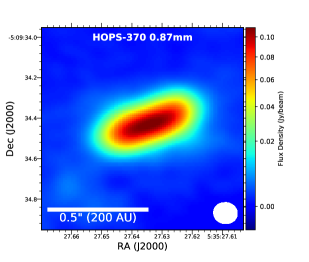
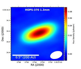
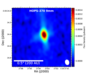
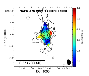
Figure 2: ALMA 0.87 mm, 1.3 mm, and VLA 9 mm continuum images of HOPS-370 and the VLA 9 mm in-band spectral index map produced by the CASA task clean. The 0.87 mm and 1.3 mm continuum emission traces an obvious disk-like structure. The 9 mm emission has extensions in the direction of the disk as well as the outflow tracing both the jet and disk emission. The contours on the 9 mm spectral index map are the VLA 9 mm continuum and are logarithmically spaced between $\pm$3$\sigma$ and 300$\sigma$, where $\sigma$=7.2 $\mu$Jy. The beam size is indicated in the lower right of each panel and is 0$\farcs$11$\times$0$\farcs$10 (43 au $\times$ 39 au), 0$\farcs$23$\times$0$\farcs$13 (90 au $\times$51 au), and 0$\farcs$08$\times$0$\farcs$07 (32 au $\times$ 28 au) at 0.87 mm, 1.3 mm, and 9 mm, respectively.

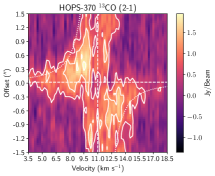
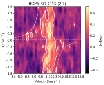
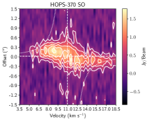
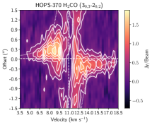
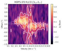
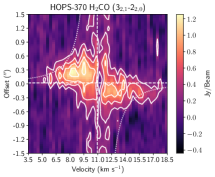
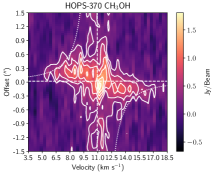
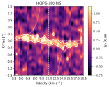
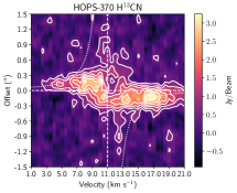
Figure 5: ALMA integrated intensity images of the molecular lines at blue- and red-shifted velocities overlaid with their corresponding contour colors and overlaid on the 0.87 mm continuum (grayscale). The red- and blue-shifted emission show a clear rotation pattern in the disk that is consistent for all molecules. The integrated intensity maps for many molecules have their emission peaks spatially located above and below the continuum emission which could be related to continuum or line opacity. The NS molecule in contrast does not seem to avoid the disk midplane. The blue-shifted images are typically integrated between 4 and 11 km s^-1, while the red-shifted images are typically integrated between 11 and 18 km s^-1. The contours plotted start at and increase on 5$\sigma$ intervals for the three H₂CO transitions, SO, and CH₃OH where $\sigma$=24 mJy beam^-1. The contour levels for the other transitions are as follows: NS starts at 3$\sigma$ and increases on 2$\sigma$ intervals and $\sigma$=38 mJy beam^-1, ¹³CO starts at 3$\sigma$ and increases on 2$\sigma$ intervals and $\sigma$=61 mJy beam^-1, C¹⁸O starts at 2$\sigma$ and increases on 1$\sigma$ intervals $\sigma$=36 mJy beam^-1, and H¹³CN starts at 4$\sigma$ and increases on 4$\sigma$ intervals and $\sigma$=33 mJy beam^-1. The green ellipse denotes the beam for the molecular line data which is $\sim$0$\farcs$23$\times$$\sim$0$\farcs$13 (90 au $\times$51 au) for all but NS and H¹³CN whose beams are 0$\farcs$15$\times$0$\farcs$14 (59 au $\times$ 55 au). The black ellipse denotes the beam for the 0.87 mm continuum data 0$\farcs$11$\times$0$\farcs$10 (43 au $\times$ 39 au).

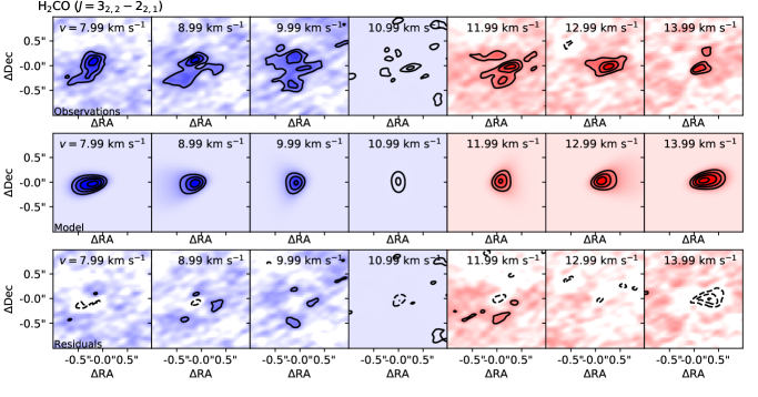
Figure 9: Figure 7b.

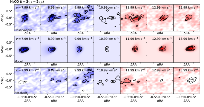
Figure 10: Figure 7c.

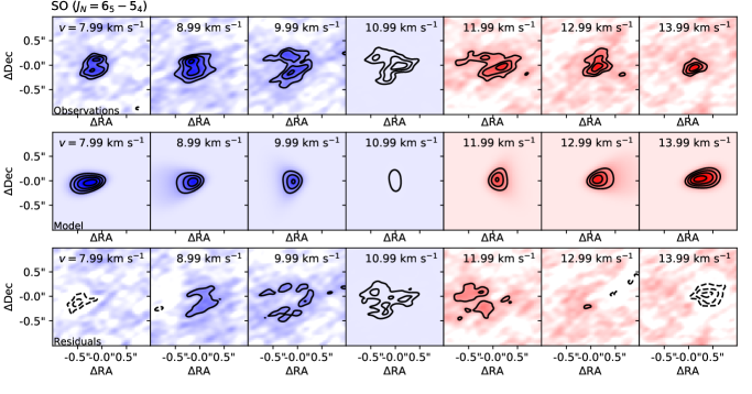
Figure 11: Figure 7d.

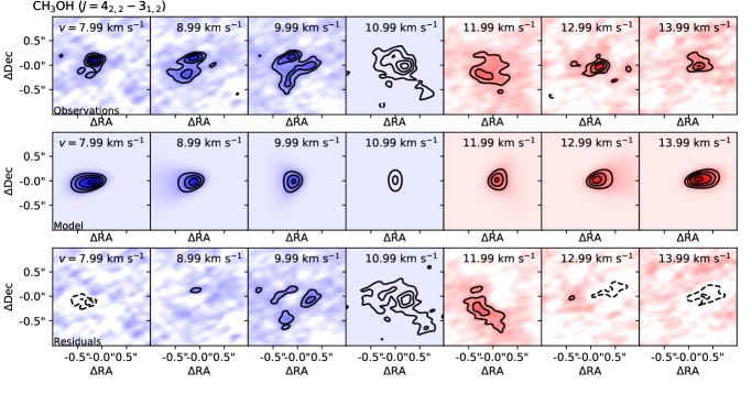
Figure 12: Figure 7e.

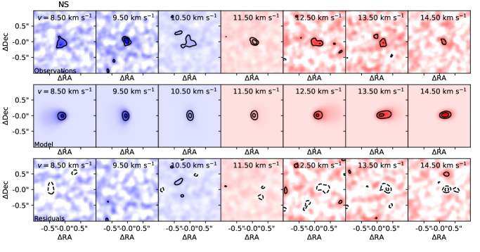
Figure 13: Figure 7f.

Figure 17: Same as Figure 7, but for models that include an envelope in the fit.

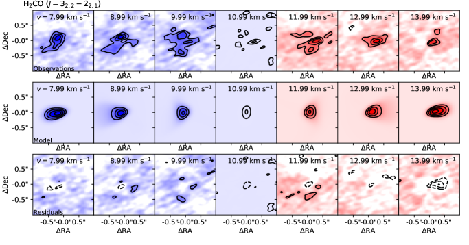
Figure 18: Figure 11b.

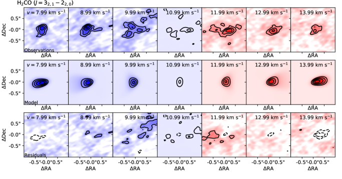
Figure 19: Figure 11c.

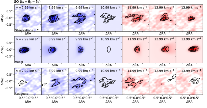
Figure 20: Figure 11d.

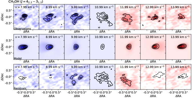
Figure 21: Figure 11e.

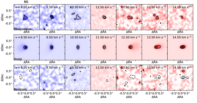
Figure 22: Figure 11f.

Table 1: Observational Setups

Telescope	Tracer	Frequency	Raw Channels	Map Channels	Image RMS	Beam	Detected?
		(GHz)	(kHz, km s-1)	(km s-1)	(mJy beam-1)	(″)
VLA	Continuum	29.0, 36.9	2000	$\cdots$	0.0072	0.08$\times$0.07	Y
ALMA Band 6	C18O ($J=2\rightarrow 1$)	219.560354	61.035, 0.083	0.5	11	0.32$\times$0.18	Y
	13CO ($J=2\rightarrow 1$)	220.398684	61.035, 0.083	0.25	23	0.32$\times$0.18	Y
	H2CO ($J=3_{0,3}\rightarrow 2_{0,2}$)	218.222192	122.07, 0.167	0.33	12	0.32$\times$0.18	Y
	H2CO ($J=3_{2,2}\rightarrow 2_{2,1}$)	218.475632	122.07, 0.167	0.33	12	0.32$\times$0.18	Y
	CH3OH ($J=4_{2,2}\rightarrow 3_{1,2}$)	218.440050	122.07, 0.167	0.33	12	0.32$\times$0.18	Y
	H2CO ($J=3_{2,1}\rightarrow 2_{2,0}$)	218.760066	122.07, 0.167	0.33	12	0.32$\times$0.18	Y
	SO ($J_{N}=6_{5}\rightarrow 5_{4}$)	219.949442	122.07, 0.167	0.33	14	0.32$\times$0.18	Y
	12CO ($J=2\rightarrow 1$)	230.538	282.23, 0.367	1.0	9.2	0.31$\times$0.17	Y
	N2D+ ($J=3\rightarrow 2$)	231.321828	282.23, 0.367	0.367	13	0.30$\times$0.17	N
	13CS ($J=5\rightarrow 4$)	231.220685	282.23, 0.367	0.366	11	0.30$\times$0.17	Y
	Continuum	232.5	31250	$\cdots$	0.22	0.23$\times$0.13	Y
ALMA Band 7	Continuum	333, 344	31250	$\cdots$	0.31	0.11$\times$0.1	Y
	NS ($J=15/2\rightarrow 13/2$, $F=17/2\rightarrow 15/2$)	346.220137	564.45, 0.489	0.5	20	0.20$\times$0.20	Y
	NS ($J=15/2\rightarrow 13/2$, $F=15/2\rightarrow 13/2$)	346.221163	564.45, 0.489	0.5	20	0.20$\times$0.20	Y
	H13CN ($J=4\rightarrow 3$)	345.3397693	564.45, 0.489	0.5	19	0.18$\times$0.17	Y
	SO2 ($J=13_{2,12}\rightarrow 12_{1,11}$)	345.3385391	564.45, 0.489	0.5	19	0.18$\times$0.17	Y

Note. — The lines contained in the ALMA Band 7 data were detected within a spectral window centered on the ¹²CO ($J=3\rightarrow 2$) transition. The spectral resolutions listed for the ALMA continuum bands are for a single channel while the full bandwidths were $\sim$1.875 GHz, also the full bandwidth for the VLA observations was 8 GHz, spilt into 2, 4 GHz bands centered at the listed frequencies. The the raw channels columns refers to the spectral resolution of the data itself, while the image channels refers to the spectral resolution after averaging during the imaging process.

Table 2: HOPS-370 Continuum Flux density

Wavelength	Flux Density	Peak Iν	RMS	Decon. Size	Decon. PA	Reference
(mm)	(mJy)	(mJy beam-1)	(mJy beam-1)	(″)	(°)
0.87	533.2$\pm$10.0	109.89	0.39	0.34$\times$0.11	109.7	1
1.3	207.4$\pm$3.0	95.7	0.22	0.32$\times$0.10	109.7	1
7.0	4.0$\pm$0.4	$\cdots$	0.015	0.24$\times$0.22	108	2
9.1	3.65$\pm$0.36	$\cdots$	$\cdots$	0.0069	$\cdots$	1
9.1 (disk-only)	0.732$\pm$0.075	0.122	0.0069	0.27$\times$0.09	112.4	1
13.0	2.6$\pm$0.3	$\cdots$	0.010	0.52$\times$0.21	7.2	2
30.0	2.16$\pm$0.22	$\cdots$	0.009	2.8$\times$1.8	30	2
50.0	1.76$\pm$0.18	$\cdots$	0.011	4.8$\times$2.6	42	2

Note. — Integrated flux densities measured toward HOPS-370. The flux densities and peak intensities from this work are derived from image-plane Gaussian fitting of HOPS-370. The 9.1 mm (disk dust-only) measurement is derived from the multi-component Gaussian fitting and this is the component that fits the disk. The other 9.1 mm flux density reflects the total integrated flux from the four component fit. Uncertainties reflect statistical uncertainties and do not include the uncertainty in the absolute flux calibration for the 0.87 mm, 1.3 mm, and 9.1 mm flux densities. The other measurements include a 10% absolute calibration uncertainty. References: (1) this work, and (2) (Osorio et al., 2017).

Table 3: VLA 9 mm Gaussian Fit

Component	RA	Dec.	Int. Flux	Peak Intensity	Deconvolved Size	PA
	(ICRS)	(ICRS)	(mJy)	(mJy beam-1)	″	(°)
Component 1 (Central Peak)	05:35:27.63360	-05:09:34.408	1.44$\pm$0.013	1.41$\pm$0.012	0.016$\times$0.007	15.9
Component 2 (Jet)	05:35:27.63422	-05.09.34.302	7.54$\pm$0.046	2.11$\pm$0.01	0.285$\times$0.021	7.0
Component 3 (Jet)	05:35:27.63438	-05.09.34.282	-6.06$\pm$0.043	-1.93$\pm$0.01	0.250$\times$0.019	7.2
Component 4 (disk)	05:35:27.63473	-05.09.34.416	0.732$\pm$0.075	0.122$\pm$0.01	0.270$\times$0.090	112.4

Note. — The individual components were fit non-interactively using the CASA task imfit. We only provided initial guesses for each component. Component 1 was constrained to have an angular size equivalent to the beam, while Components 2 and 3 had initial parameter estimates elogated in their fitted directions, but without restrictions on their angular size or position angle. Then Component 4 was provided with an initial position angle and angular size consistent with the expected disk, but the Gaussian parameters were also not fixed for Component 4. Component 4 is thus taken to provide an estimate of the flux density from the dust emission from the disk at 9 mm. The fact that Component 2 has a large positive flux density and Component 3 has a large negative flux density is not important, the combination of these two components fits the jet morphology well. The sum of the flux densites from all componets agrees well the the total flux density measured within a polygon and the flux density from Osorio et al. (2017).

Table 4: Molecular Line Modeling Parameters

Parameter Description	Parameter	Parameter Range
Stellar Mass	$M_{*}$ (M☉)	0.1 - 10.0
Disk Mass	$M_{disk}$ (M☉)	0.01 - 1.0
Disk Outer Radius	$r_{c}$ (au)	1.0 - 10000.0
Disk Inner Radius	$R_{in,disk}$ (au)	0.1
Surface Density Power-law Index	$\gamma$	0.0 - 2.0
Disk Vertical Density Profile	$h(r)$	HSEQ
Temperature at 1 au	$T_{0}$ (K)	10.0 - 1000.0
Temperature Profile Power-law Index	$q$	0.35 (0.0 - 1.0)
Envelope Mass	$M_{env}$ (M☉)	0 - 10.0
Envelope Outer Radius	$R_{env}$ (au)	1000.0 - 10000.0
Envelope Inner Radius	$R_{in,env}$ (au)	0.1
Centrifugal Radius	$R_{c}$ (au)	=$R_{disk}$
Turbulent velocity Width	$a$ (km s-1)	0.001 - 0.13
Inclination	$i$ (°)	72.2
Density Scaling in Outflow Cavity	$f_{cav}$	0.5
Outflow Cavity Shape power-law index	$\xi$	1.0
Right Ascension Offset	$\Delta$x (″)	-0.2 - 0.2
Declination Offset	$\Delta$y (″)	-0.2 - 0.2
Distance	d (pc)	400.0
Position Angle East of North	$pa$ (°)	310 - 380
System Velocity	$v_{sys}$ (km s-1)	7.0 - 15.0
H2CO Abundnace	(per H2)	1.0$\times$10-9
SO Abundance	(per H2)	3.14$\times$10-9 (1.0$\times$10-8 - 1.0$\times$10-10)
CH3OH Abundance	(per H2)	1.0$\times$10-8 (1.0$\times$10-7 - 1.0$\times$10-10)
NS Abundance	(per H2)	13.14$\times$10-9 (1.0$\times$10-8 - 1.0$\times$10-10)

Note. — The disk and envelope parameters were varied (range) and fixed (single value) for the molecular line modeling. For $q$ and the SO abundance, we explored the effects of having these parameters fixed for most runs, but allowed them to vary in a few specific instances that are described in the text: hence the single value and range of values in parentheses. More explanation of the parameters and the model setup is provided in Section 4.1. The parameter f_cav is the reduction of envelope density within the outflow cavity, and the outflow cavity shape and opening angle are defined by the parameter $\xi$, translating to opening angle can be done by calculating 2tan^-1($\xi$).

Table 5: HOPS-370 Molecular Line Models - Exponentially Tapered Disks without Envelope

Transition(s)	Mass	Disk Radius	Disk Mass	Vlsr	Pos. Angle	$\Delta$x	$\Delta$y	$\gamma$	T(1 au)	q	$log_{10}$(Mol./H2)
	(M☉)	(AU)	(M☉)	(km s-1)	°	(″)	(″)		(K)
H2CO ($J=3_{0,3}\rightarrow 2_{0,2}$)	2.72$\pm$0.03	82.28$\pm$0.7	0.31$\pm$0.004	11.07$\pm$0.02	353.86$\pm$0.34	0.004$\pm$0.002	0.022$\pm$0.002	1.08$\pm$0.01	995.92$\pm$5.59	0.35	$\cdots$
H2CO (2 lines)	2.33$\pm$0.03	82.79$\pm$0.8	0.43$\pm$0.007	11.08$\pm$0.01	352.69$\pm$0.39	0.011$\pm$0.002	0.012$\pm$0.002	1.16$\pm$0.02	998.06$\pm$1.72	0.35	$\cdots$
H2CO (3 lines)	2.52$\pm$0.02	82.99$\pm$1.5	0.54$\pm$0.012	11.09$\pm$0.01	352.64$\pm$0.25	0.006$\pm$0.001	0.014$\pm$0.001	1.10$\pm$0.02	998.82$\pm$1.63	0.35	$\cdots$
CH3OH ($J=4_{2,2}\rightarrow 3_{1,2}$)	2.37$\pm$0.03	109.29$\pm$1.3	0.39$\pm$0.007	10.99$\pm$0.02	358.02$\pm$0.58	0.010$\pm$0.002	0.004$\pm$0.002	0.89$\pm$0.02	998.70$\pm$1.89	0.35	$\cdots$
CH3OH, H2CO (3 lines)	2.50$\pm$0.02	90.36$\pm$1.0	0.49$\pm$0.007	11.06$\pm$0.01	353.45$\pm$0.24	0.007$\pm$0.001	0.013$\pm$0.001	1.05$\pm$0.01	998.38$\pm$1.09	0.35	-0.88$\pm$0.013
SO ($J_{N}=6_{5}\rightarrow 5_{4}$)	2.51$\pm$0.05	104.78$\pm$2.1	0.19$\pm$0.005	11.42$\pm$0.03	345.10$\pm$0.74	0.023$\pm$0.002	0.041$\pm$0.002	0.80$\pm$0.03	999.21$\pm$1.11	0.35	$\cdots$
SO and CH3OH	2.37$\pm$0.04	120.53$\pm$0.9	0.29$\pm$0.005	11.03$\pm$0.03	353.00$\pm$0.58	0.011$\pm$0.002	0.029$\pm$0.002	0.67$\pm$0.02	998.44$\pm$1.85	0.35	-0.88$\pm$0.005
SO, H2CO (3 lines)	2.55$\pm$0.02	99.29$\pm$0.3	0.42$\pm$0.003	11.12$\pm$0.01	351.46$\pm$0.24	0.009$\pm$0.001	0.018$\pm$0.001	0.93$\pm$0.01	999.63$\pm$0.47	0.35	-2.84$\pm$0.203
NS	3.63$\pm$0.16	79.77$\pm$20.8	0.01$\pm$0.006	11.05$\pm$0.09	350.56$\pm$1.69	-0.007$\pm$0.004	0.014$\pm$0.004	0.31$\pm$0.24	776.35$\pm$246.00	0.35	$\cdots$
NS, SO	1.83$\pm$0.03	82.87$\pm$1.3	0.02$\pm$0.001	10.98$\pm$0.03	352.76$\pm$0.54	0.016$\pm$0.002	0.062$\pm$0.001	1.06$\pm$0.02	998.44$\pm$1.23	0.35	-0.88$\pm$0.011
NS, CH3OH	2.44$\pm$0.03	109.43$\pm$1.7	0.38$\pm$0.008	11.00$\pm$0.02	356.56$\pm$0.56	0.008$\pm$0.002	0.006$\pm$0.002	0.89$\pm$0.02	996.65$\pm$3.85	0.35	-0.88$\pm$0.018
NS, H2CO (3 lines)	2.56$\pm$0.02	88.86$\pm$1.1	0.50$\pm$0.008	11.09$\pm$0.01	352.46$\pm$0.27	0.007$\pm$0.001	0.014$\pm$0.001	1.06$\pm$0.01	998.87$\pm$1.23	0.35	-0.88$\pm$0.012
H2CO (3 lines, q fit)	2.37$\pm$0.02	69.69$\pm$0.6	1.00$\pm$0.003	11.13$\pm$0.01	353.76$\pm$0.31	0.001$\pm$0.001	0.009$\pm$0.001	1.39$\pm$0.01	997.92$\pm$2.28	0.001$\pm$0.001	$\cdots$

Note. — The results from each model lists the molecular line(s) fit with the pdspy models. For H₂CO, ‘3 lines’, refers to all three ($J=3_{n,n}\rightarrow 2_{n,n}$) transitions, while ‘2 lines’ refers to the higher excitation ($J=3_{2,2}\rightarrow 2_{2,1}$) and ($J=3_{2,1}\rightarrow 2_{2,0}$) transitions (see Table 1). The parameter $q$, the power-law index of the disk temperature profile is fixed for all models except when ‘q fit’ is listed in the description. The Mass column refers to the protostar mass, $\Delta x$ and $\Delta y$ refer to the offset of the model center of mass with respect to the image phase center, $\gamma$ is the power-law index of the disk surface density profile, and SO Abund. refers to the SO abundance adopted or fit by the models.

Table 6: HOPS-370 Continuum Modeling Results

Parameter Description	Parameter	Fit Value
System Luminosity	$L_{*}$ (L☉)	$279.9^{+14.1}_{-13.1}$
Disk Mass	$M_{disk}$ (M☉)	$0.035^{+0.005}_{-0.003}$
Disk Outer Radius	$R_{disk}$ (au)	$61.9^{+0.7}_{-1.2}$
Disk Inner Radius	$R_{in,disk}$ (au)	$0.54^{+0.27}_{-0.09}$
Envelope Mass	$M_{env}$ (M☉)	$0.12^{+0.01}_{-0.01}$
Envelope Radius	$R_{env}$ (au)	$1881^{+78}_{-137}$
Envelope Inner Radius	$R_{in,env}$ (au)	=$R_{in,disk}$
Envelope Centrifugal Radius	$R_{c}$ (au)	=$R_{disk}$
Surface Density Power-law Index	$\gamma$	$-0.47^{+0.02}_{-0.01}$
Flaring Power-law Index	$\beta$	$0.66^{+0.02}_{-0.03}$
Scale Height at 1 au	$h_{0}$ (au)	$0.132^{+0.009}_{-0.008}$
Inclination	$i$	$74.0^{+0.2}_{-0.2}$
Density Scaling in Outflow Cavity	$f_{cav}$	$0.33^{+0.01}_{-0.02}$
Outflow Cavity Shape power-law index	$\xi$	$1.12^{+0.06}_{-0.05}$
Maximum dust grain size	$a_{max}$ (µm)	$432^{+31}_{-47}$
Dust grain size distribution power-law index	$p$	$2.63^{+0.04}_{-0.06}$
Position Angle East of North	$pa$ (°)	$109.7^{+0.1}_{-0.2}$
Distance	d (pc)	400.0

Note. — The disk and envelope parameters derived from continuum modeling are reported here. More explanation of the parameters is provided in Sections 4.1 and 4.2. However, we explain a few that are less intuitive. The parameter f_cav is the reduction of envelope density within the outflow cavity, and the outflow cavity shape and opening angle are defined by the parameter $\xi$, translating to opening angle can be done by calculating 2tan^-1($\xi$), corresponding to a full opening angle of $\sim$98°. The maximum dust size and grain size distribution are defined by a_max and p, where the dust grain size distribution follows a power-law n(a)^-p. Absolute flux calibration uncertainty was not taken into account in the modeling.

Table 7: HOPS-370 Molecular Line Models - Exponentially Tapered Disks with Envelope

Transition(s)	Mass	Disk Radius	Disk Mass	Envelope Radius	Envelope Mass	Vlsr	Pos. Angle	$\Delta$x	$\Delta$y	$\gamma$	T(1 au)	q	$log_{10}$(Mol./H2)
	(M☉)	(AU)	(M☉)	(AU)	(M☉)	(km s-1)	°	(″)	(″)		(K)
H2CO ($J=3_{0,3}\rightarrow 2_{0,2}$)	2.81$\pm$0.03	32.97$\pm$3.3	0.77$\pm$0.070	8345.89$\pm$8536.0	0.548$\pm$0.660	11.19$\pm$0.02	353.35$\pm$0.34	-0.000$\pm$0.002	0.015$\pm$0.001	1.32$\pm$0.02	997.43$\pm$3.76	0.35	$\cdots$
H2CO (2 lines)	2.46$\pm$0.03	36.07$\pm$4.1	0.85$\pm$0.075	1081.80$\pm$182.1	0.049$\pm$0.010	11.21$\pm$0.02	352.00$\pm$0.44	0.011$\pm$0.002	0.004$\pm$0.002	1.37$\pm$0.03	998.69$\pm$1.66	0.35	$\cdots$
H2CO (3 lines)	2.66$\pm$0.02	62.99$\pm$3.1	0.69$\pm$0.034	1076.49$\pm$21.0	0.071$\pm$0.004	11.20$\pm$0.01	352.39$\pm$0.28	0.006$\pm$0.001	0.009$\pm$0.001	1.16$\pm$0.02	999.52$\pm$0.66	0.35	$\cdots$
CH3OH ($J=4_{2,2}\rightarrow 3_{1,2}$)	2.46$\pm$0.03	81.51$\pm$5.6	0.51$\pm$0.035	1009.67$\pm$20.1	0.037$\pm$0.004	11.07$\pm$0.02	357.55$\pm$0.54	0.012$\pm$0.002	-0.001$\pm$0.002	1.08$\pm$0.04	998.72$\pm$1.91	0.35	$\cdots$
CH3OH, H2CO (3 lines)	2.60$\pm$0.02	74.65$\pm$2.5	0.57$\pm$0.019	1013.96$\pm$29.7	0.054$\pm$0.002	11.14$\pm$0.01	353.58$\pm$0.22	0.007$\pm$0.001	0.008$\pm$0.001	1.09$\pm$0.02	999.09$\pm$0.85	0.35	-7.99$\pm$0.005
SO ($J_{N}=6_{5}\rightarrow 5_{4}$)	2.63$\pm$0.04	90.16$\pm$4.1	0.23$\pm$0.011	1013.35$\pm$15.2	0.013$\pm$0.001	11.53$\pm$0.02	344.85$\pm$0.61	0.024$\pm$0.002	0.036$\pm$0.002	1.00$\pm$0.05	999.36$\pm$0.73	0.35	$\cdots$
SO and CH3OH	2.35$\pm$0.04	113.69$\pm$2.9	0.30$\pm$0.012	1067.64$\pm$35.0	0.023$\pm$0.003	11.12$\pm$0.03	352.97$\pm$0.65	0.013$\pm$0.001	0.026$\pm$0.002	0.65$\pm$0.04	993.91$\pm$3.08	0.35	-8.70$\pm$0.007
SO, H2CO (3 lines)	2.63$\pm$0.02	85.17$\pm$2.4	0.50$\pm$0.015	5466.58$\pm$202.3	0.320$\pm$0.026	11.19$\pm$0.01	351.38$\pm$0.23	0.009$\pm$0.001	0.015$\pm$0.001	1.02$\pm$0.02	999.23$\pm$0.88	0.35	-8.76$\pm$0.005
NS	3.83$\pm$0.15	55.96$\pm$26.9	0.03$\pm$0.018	5889.31$\pm$3114.6	0.046$\pm$0.067	11.01$\pm$0.07	350.24$\pm$1.52	-0.010$\pm$0.004	0.013$\pm$0.003	0.55$\pm$0.35	424.31$\pm$38.63	0.35	$\cdots$
NS, SO	1.85$\pm$0.03	14.17$\pm$2.2	0.06$\pm$0.004	4671.31$\pm$117.8	0.006$\pm$0.002	11.10$\pm$0.03	353.53$\pm$0.55	0.018$\pm$0.002	0.060$\pm$0.002	1.57$\pm$0.02	998.54$\pm$1.37	0.35	-7.50$\pm$0.002
NS, CH3OH	2.52$\pm$0.04	88.72$\pm$6.8	0.46$\pm$0.035	1074.55$\pm$180.6	0.029$\pm$0.007	11.07$\pm$0.03	356.83$\pm$0.66	0.009$\pm$0.003	0.004$\pm$0.002	1.04$\pm$0.05	991.41$\pm$4.22	0.35	-9.77$\pm$0.018
NS, H2CO (3 lines)	2.67$\pm$0.02	78.74$\pm$2.7	0.55$\pm$0.021	5475.02$\pm$481.8	0.532$\pm$0.066	11.17$\pm$0.01	352.43$\pm$0.31	0.006$\pm$0.001	0.010$\pm$0.001	1.07$\pm$0.02	998.17$\pm$1.80	0.35	-9.82$\pm$0.018
H2CO (3 lines, q fit)	2.57$\pm$0.02	52.98$\pm$0.9	0.99$\pm$0.011	1054.51$\pm$15.0	0.18$\pm$0.005	11.33$\pm$0.01	352.71$\pm$0.26	0.004$\pm$0.001	0.003$\pm$0.001	1.27$\pm$0.01	998.85$\pm$1.46	0.0003$\pm$0.0005	$\cdots$

Note. — The results from each model lists the molecular line(s) fit with the pdspy models. For H₂CO, ‘3 lines’, refers to all three ($J=3_{n,n}\rightarrow 2_{n,n}$) transitions, while ‘2 lines’ refers to the higher excitation ($J=3_{2,2}\rightarrow 2_{2,1}$) and ($J=3_{2,1}\rightarrow 2_{2,0}$) transitions (see Table 1). The parameter $q$, the power-law index of the disk temperature profile is fixed for all models except when ‘q fit’ is listed in the description. The Mass column refers to the protostar mass, $\Delta x$ and $\Delta y$ refer to the offset of the model center of mass with respect to the image phase center, $\gamma$ is the power-law index of the disk surface density profile, and SO Abund. refers to the SO abundance adopted or fit by the models.

References

- Adams et al. (1989) Adams, F. C., Ruden, S. P., & Shu, F. H. 1989, ApJ, 347, 959, doi: 10.1086/168187
- Adams et al. (2012) Adams, J. D., Herter, T. L., Osorio, M., et al. 2012, ApJ, 749, L24, doi: 10.1088/2041-8205/749/2/L24
- Alcalá et al. (2017) Alcalá, J. M., Manara, C. F., Natta, A., et al. 2017, A&A, 600, A20, doi: 10.1051/0004-6361/201629929
- Allen et al. (2003) Allen, A., Li, Z., & Shu, F. H. 2003, ApJ, 599, 363, doi: 10.1086/379243
- André et al. (1993) André, P., Ward-Thompson, D., & Barsony, M. 1993, ApJ, 406, 122, doi: 10.1086/172425
- Anglada et al. (1998) Anglada, G., Villuendas, E., Estalella, R., et al. 1998, AJ, 116, 2953, doi: 10.1086/300637
- Ansdell et al. (2018) Ansdell, M., Williams, J. P., Trapman, L., et al. 2018, ArXiv e-prints. https://arxiv.org/abs/1803.05923
- Aso et al. (2017) Aso, Y., Ohashi, N., Aikawa, Y., et al. 2017, ArXiv e-prints. https://arxiv.org/abs/1707.08697
- Astropy Collaboration et al. (2018) Astropy Collaboration, Price-Whelan, A. M., Sipőcz, B. M., et al. 2018, The Astropy Project: Building an Open-science Project and Status of the v2.0 Core Package, doi: 10.3847/1538-3881/aabc4f
- Audard et al. (2014) Audard, M., Ábrahám, P., Dunham, M. M., et al. 2014, in Protostars and Planets VI, ed. H. Beuther, R. S. Klessen, C. P. Dullemond, & T. Henning, 387
- Bae et al. (2015) Bae, J., Hartmann, L., & Zhu, Z. 2015, ArXiv e-prints. https://arxiv.org/abs/1503.02694
- Bai & Stone (2013) Bai, X.-N., & Stone, J. M. 2013, ApJ, 769, 76, doi: 10.1088/0004-637X/769/1/76
- Balbus & Hawley (1991) Balbus, S. A., & Hawley, J. F. 1991, ApJ, 376, 214, doi: 10.1086/170270
- Baraffe et al. (2009) Baraffe, I., Chabrier, G., & Gallardo, J. 2009, ApJ, 702, L27, doi: 10.1088/0004-637X/702/1/L27
- Bate (2012) Bate, M. R. 2012, MNRAS, 419, 3115, doi: 10.1111/j.1365-2966.2011.19955.x
- Birnstiel et al. (2010) Birnstiel, T., Dullemond, C. P., & Brauer, F. 2010, A&A, 513, A79, doi: 10.1051/0004-6361/200913731
- Bohlin et al. (1978) Bohlin, R. C., Savage, B. D., & Drake, J. F. 1978, ApJ, 224, 132, doi: 10.1086/156357
- Bonnell et al. (2001) Bonnell, I. A., Bate, M. R., Clarke, C. J., & Pringle, J. E. 2001, MNRAS, 323, 785, doi: 10.1046/j.1365-8711.2001.04270.x
- Calvet et al. (1991) Calvet, N., Patino, A., Magris, G. C., & D’Alessio, P. 1991, ApJ, 380, 617, doi: 10.1086/170618
- Cassen & Moosman (1981) Cassen, P., & Moosman, A. 1981, Icarus, 48, 353, doi: 10.1016/0019-1035(81)90051-8
- Ceccarelli (2004) Ceccarelli, C. 2004, in Astronomical Society of the Pacific Conference Series, Vol. 323, Star Formation in the Interstellar Medium: In Honor of David Hollenbach, ed. D. Johnstone, F. C. Adams, D. N. C. Lin, D. A. Neufeeld, & E. C. Ostriker, 195
- Chandler et al. (1995) Chandler, C. J., Carlstrom, J. E., & Scoville, N. Z. 1995, ApJ, 446, 793, doi: 10.1086/175836
- Chen et al. (1995) Chen, H., Myers, P. C., Ladd, E. F., & Wood, D. O. S. 1995, ApJ, 445, 377, doi: 10.1086/175703
- Chini et al. (1997) Chini, R., Reipurth, B., Sievers, A., et al. 1997, A&A, 325, 542
- Connelley & Greene (2010) Connelley, M. S., & Greene, T. P. 2010, AJ, 140, 1214, doi: 10.1088/0004-6256/140/5/1214
- Connelley et al. (2009) Connelley, M. S., Reipurth, B., & Tokunaga, A. T. 2009, AJ, 138, 1193, doi: 10.1088/0004-6256/138/5/1193
- Crockett et al. (2014) Crockett, N. R., Bergin, E. A., Neill, J. L., et al. 2014, ApJ, 787, 112, doi: 10.1088/0004-637X/787/2/112
- Cushing et al. (2004) Cushing, M. C., Vacca, W. D., & Rayner, J. T. 2004, PASP, 116, 362, doi: 10.1086/382907
- Dapp & Basu (2010) Dapp, W. B., & Basu, S. 2010, A&A, 521, L56+, doi: 10.1051/0004-6361/201015700
- Drozdovskaya et al. (2016) Drozdovskaya, M. N., Walsh, C., van Dishoeck, E. F., et al. 2016, MNRAS, 462, 977, doi: 10.1093/mnras/stw1632
- Dullemond et al. (2012) Dullemond, C. P., Juhasz, A., Pohl, A., et al. 2012, RADMC-3D: A multi-purpose radiative transfer tool. http://ascl.net/1202.015
- Dunham et al. (2010) Dunham, M. M., Evans, N. J., Terebey, S., Dullemond, C. P., & Young, C. H. 2010, ApJ, 710, 470, doi: 10.1088/0004-637X/710/1/470
- Dunham et al. (2014a) Dunham, M. M., Vorobyov, E. I., & Arce, H. G. 2014a, MNRAS, 444, 887, doi: 10.1093/mnras/stu1511
- Dunham et al. (2014b) Dunham, M. M., Stutz, A. M., Allen, L. E., et al. 2014b, Protostars and Planets VI, 195, doi: 10.2458/azu_uapress_9780816531240-ch009
- Emprechtinger et al. (2009) Emprechtinger, M., Caselli, P., Volgenau, N. H., Stutzki, J., & Wiedner, M. C. 2009, A&A, 493, 89, doi: 10.1051/0004-6361:200810324
- Feng et al. (2016) Feng, S., Beuther, H., Semenov, D., et al. 2016, A&A, 593, A46, doi: 10.1051/0004-6361/201424912
- Fischer et al. (2012) Fischer, W. J., Megeath, S. T., Tobin, J. J., et al. 2012, ApJ, 756, 99, doi: 10.1088/0004-637X/756/1/99
- Fischer et al. (2017) Fischer, W. J., Megeath, S. T., Furlan, E., et al. 2017, ApJ, 840, 69, doi: 10.3847/1538-4357/aa6d69
- Foreman-Mackey et al. (2013) Foreman-Mackey, D., Hogg, D. W., Lang, D., & Goodman, J. 2013, PASP, 125, 306, doi: 10.1086/670067
- Frank et al. (2014) Frank, A., Ray, T. P., Cabrit, S., et al. 2014, ArXiv e-prints. https://arxiv.org/abs/1402.3553
- Furlan et al. (2014) Furlan, E., Megeath, S. T., Osorio, M., et al. 2014, ApJ, 786, 26, doi: 10.1088/0004-637X/786/1/26
- Furlan et al. (2016) Furlan, E., Fischer, W. J., Ali, B., et al. 2016, ApJS, 224, 5, doi: 10.3847/0067-0049/224/1/5
- Gammie (1996) Gammie, C. F. 1996, ApJ, 457, 355, doi: 10.1086/176735
- Gerner et al. (2014) Gerner, T., Beuther, H., Semenov, D., et al. 2014, A&A, 563, A97, doi: 10.1051/0004-6361/201322541
- González-García et al. (2016) González-García, B., Manoj, P., Watson, D. M., et al. 2016, A&A, 596, A26, doi: 10.1051/0004-6361/201527186
- Greenfield et al. (2013) Greenfield, P., Robitaille, T., Tollerud, E., et al. 2013. http://ascl.net/1304.002
- Harsono et al. (2014) Harsono, D., Jørgensen, J. K., van Dishoeck, E. F., et al. 2014, A&A, 562, A77, doi: 10.1051/0004-6361/201322646
- Hartmann (2008) Hartmann, L. 2008, Physica Scripta Volume T, 130, 014012, doi: 10.1088/0031-8949/2008/T130/014012
- Hartmann et al. (1996) Hartmann, L., Calvet, N., & Boss, A. 1996, ApJ, 464, 387, doi: 10.1086/177330
- Hosokawa et al. (2010) Hosokawa, T., Yorke, H. W., & Omukai, K. 2010, ApJ, 721, 478, doi: 10.1088/0004-637X/721/1/478
- Hsu et al. (2010) Hsu, W., Hartmann, L., Heitsch, F., & Gómez, G. C. 2010, ApJ, 721, 1531, doi: 10.1088/0004-637X/721/2/1531
- Ingleby et al. (2013) Ingleby, L., Calvet, N., Herczeg, G., et al. 2013, ApJ, 767, 112, doi: 10.1088/0004-637X/767/2/112
- Isella & Turner (2018) Isella, A., & Turner, N. J. 2018, ApJ, 860, 27, doi: 10.3847/1538-4357/aabb07
- Jacobsen et al. (2018) Jacobsen, S. K., Jørgensen, J. K., Di Francesco, J., et al. 2018, arXiv e-prints, arXiv:1809.00390. https://arxiv.org/abs/1809.00390
- Joos et al. (2012) Joos, M., Hennebelle, P., & Ciardi, A. 2012, A&A, 543, A128, doi: 10.1051/0004-6361/201118730
- Jørgensen et al. (2009) Jørgensen, J. K., van Dishoeck, E. F., Visser, R., et al. 2009, A&A, 507, 861, doi: 10.1051/0004-6361/200912325
- Kainulainen et al. (2017) Kainulainen, J., Stutz, A. M., Stanke, T., et al. 2017, A&A, 600, A141, doi: 10.1051/0004-6361/201628481
- Kama et al. (2020) Kama, M., Trapman, L., Fedele, D., et al. 2020, A&A, 634, A88, doi: 10.1051/0004-6361/201937124
- Keppler et al. (2018) Keppler, M., Benisty, M., Müller, A., et al. 2018, A&A, 617, A44, doi: 10.1051/0004-6361/201832957
- Konigl & Pudritz (2000) Konigl, A., & Pudritz, R. E. 2000, Protostars and Planets IV, 759
- Kounkel et al. (2016) Kounkel, M., Megeath, S. T., Poteet, C. A., Fischer, W. J., & Hartmann, L. 2016, ApJ, 821, 52, doi: 10.3847/0004-637X/821/1/52
- Kounkel et al. (2018) Kounkel, M., Covey, K., Suárez, G., et al. 2018, AJ, 156, 84, doi: 10.3847/1538-3881/aad1f1
- Kratter & Lodato (2016) Kratter, K., & Lodato, G. 2016, ARA&A, 54, 271, doi: 10.1146/annurev-astro-081915-023307
- Lee et al. (2018) Lee, C.-F., Li, Z.-Y., Codella, C., et al. 2018, ApJ, 856, 14, doi: 10.3847/1538-4357/aaae6d
- Lesur et al. (2015) Lesur, G., Hennebelle, P., & Fromang, S. 2015, A&A, 582, L9, doi: 10.1051/0004-6361/201526734
- Li et al. (2014) Li, Z.-Y., Banerjee, R., Pudritz, R. E., et al. 2014, Protostars and Planets VI, 173, doi: 10.2458/azu_uapress_9780816531240-ch008
- Lodders (2003) Lodders, K. 2003, ApJ, 591, 1220, doi: 10.1086/375492
- López-Sepulcre et al. (2013) López-Sepulcre, A., Taquet, V., Sánchez-Monge, Á., et al. 2013, A&A, 556, A62, doi: 10.1051/0004-6361/201220905
- Lynden-Bell & Pringle (1974) Lynden-Bell, D., & Pringle, J. E. 1974, MNRAS, 168, 603, doi: 10.1093/mnras/168.3.603
- Manoj et al. (2013) Manoj, P., Watson, D. M., Neufeld, D. A., et al. 2013, ApJ, 763, 83, doi: 10.1088/0004-637X/763/2/83
- Masson et al. (2016) Masson, J., Chabrier, G., Hennebelle, P., Vaytet, N., & Commerçon, B. 2016, A&A, 587, A32, doi: 10.1051/0004-6361/201526371
- McKee & Tan (2003) McKee, C. F., & Tan, J. C. 2003, ApJ, 585, 850, doi: 10.1086/346149
- McMullin et al. (2007) McMullin, J. P., Waters, B., Schiebel, D., Young, W., & Golap, K. 2007, in Astronomical Society of the Pacific Conference Series, Vol. 376, Astronomical Data Analysis Software and Systems XVI, ed. R. A. Shaw, F. Hill, & D. J. Bell, 127
- Megeath et al. (2012) Megeath, S. T., Gutermuth, R., Muzerolle, J., et al. 2012, AJ, 144, 192, doi: 10.1088/0004-6256/144/6/192
- Mellon & Li (2008) Mellon, R. R., & Li, Z.-Y. 2008, ApJ, 681, 1356, doi: 10.1086/587542
- Murillo & Lai (2013) Murillo, N. M., & Lai, S.-P. 2013, ApJ, 764, L15, doi: 10.1088/2041-8205/764/1/L15
- Muzerolle et al. (1998) Muzerolle, J., Hartmann, L., & Calvet, N. 1998, AJ, 116, 2965, doi: 10.1086/300636
- Najita et al. (1996) Najita, J., Carr, J. S., Glassgold, A. E., Shu, F. H., & Tokunaga, A. T. 1996, ApJ, 462, 919, doi: 10.1086/177205
- Nielbock et al. (2003) Nielbock, M., Chini, R., & Müller, S. A. H. 2003, A&A, 408, 245, doi: 10.1051/0004-6361:20030961
- Offner et al. (2019) Offner, S. S. R., Gaches, B. A. L., & Holdship, J. R. 2019, ApJ, 883, 121, doi: 10.3847/1538-4357/ab3e02
- Offner et al. (2012) Offner, S. S. R., Robitaille, T. P., Hansen, C. E., McKee, C. F., & Klein, R. I. 2012, ApJ, 753, 98, doi: 10.1088/0004-637X/753/2/98
- Ohashi et al. (2014) Ohashi, N., Saigo, K., Aso, Y., et al. 2014, ApJ, 796, 131, doi: 10.1088/0004-637X/796/2/131
- Osorio et al. (2017) Osorio, M., Díaz-Rodríguez, A. K., Anglada, G., et al. 2017, ApJ, 840, 36, doi: 10.3847/1538-4357/aa6975
- Ossenkopf & Henning (1994) Ossenkopf, V., & Henning, T. 1994, A&A, 291, 943
- Oya et al. (2015) Oya, Y., Sakai, N., Lefloch, B., et al. 2015, ApJ, 812, 59, doi: 10.1088/0004-637X/812/1/59
- Palla & Stahler (1993) Palla, F., & Stahler, S. W. 1993, ApJ, 418, 414, doi: 10.1086/173402
- Pinilla et al. (2012) Pinilla, P., Birnstiel, T., Ricci, L., et al. 2012, A&A, 538, A114, doi: 10.1051/0004-6361/201118204
- Pinte et al. (2018) Pinte, C., Price, D. J., Ménard, F., et al. 2018, ApJ, 860, L13, doi: 10.3847/2041-8213/aac6dc
- Pollack et al. (1994) Pollack, J. B., Hollenbach, D., Beckwith, S., et al. 1994, ApJ, 421, 615, doi: 10.1086/173677
- Pudritz & Norman (1983) Pudritz, R. E., & Norman, C. A. 1983, ApJ, 274, 677, doi: 10.1086/161481
- Pudritz et al. (2007) Pudritz, R. E., Ouyed, R., Fendt, C., & Brandenburg, A. 2007, in Protostars and Planets V, ed. B. Reipurth, D. Jewitt, & K. Keil, 277
- Reipurth et al. (1999) Reipurth, B., Rodríguez, L. F., & Chini, R. 1999, AJ, 118, 983, doi: 10.1086/300958
- Rice et al. (2010) Rice, W. K. M., Mayo, J. H., & Armitage, P. J. 2010, MNRAS, 402, 1740, doi: 10.1111/j.1365-2966.2009.15992.x
- Robitaille & Bressert (2012) Robitaille, T., & Bressert, E. 2012, APLpy: Astronomical Plotting Library in Python, Astrophysics Source Code Library. http://ascl.net/1208.017
- Robitaille et al. (2006) Robitaille, T. P., Whitney, B. A., Indebetouw, R., Wood, K., & Denzmore, P. 2006, ApJS, 167, 256, doi: 10.1086/508424
- Safron et al. (2015) Safron, E. J., Fischer, W. J., Megeath, S. T., et al. 2015, ApJ, 800, L5, doi: 10.1088/2041-8205/800/1/L5
- Sakai et al. (2014) Sakai, N., Oya, Y., Sakai, T., et al. 2014, ApJ, 791, L38, doi: 10.1088/2041-8205/791/2/L38
- Schöier et al. (2002) Schöier, F. L., Jørgensen, J. K., van Dishoeck, E. F., & Blake, G. A. 2002, A&A, 390, 1001, doi: 10.1051/0004-6361:20020756
- Segura-Cox et al. (2016) Segura-Cox, D. M., Harris, R. J., Tobin, J. J., et al. 2016, ApJ, 817, L14, doi: 10.3847/2041-8205/817/2/L14
- Seifried et al. (2013) Seifried, D., Banerjee, R., Pudritz, R. E., & Klessen, R. S. 2013, MNRAS, 432, 3320, doi: 10.1093/mnras/stt682
- Shakura & Syunyaev (1973) Shakura, N. I., & Syunyaev, R. A. 1973, A&A, 24, 337
- Sheehan & Eisner (2014) Sheehan, P. D., & Eisner, J. A. 2014, ApJ, 791, 19, doi: 10.1088/0004-637X/791/1/19
- Sheehan & Eisner (2017) —. 2017, ApJ, 851, 45, doi: 10.3847/1538-4357/aa9990
- Sheehan et al. (2019) Sheehan, P. D., Wu, Y.-L., Eisner, J. A., & Tobin, J. J. 2019, ApJ, 874, 136, doi: 10.3847/1538-4357/ab09f9
- Shimajiri et al. (2008) Shimajiri, Y., Takahashi, S., Takakuwa, S., Saito, M., & Kawabe, R. 2008, ApJ, 683, 255, doi: 10.1086/588629
- Shu et al. (1994) Shu, F., Najita, J., Ostriker, E., et al. 1994, ApJ, 429, 781, doi: 10.1086/174363
- Takahashi et al. (2008) Takahashi, S., Saito, M., Ohashi, N., et al. 2008, ApJ, 688, 344, doi: 10.1086/592212
- Taquet et al. (2015) Taquet, V., López-Sepulcre, A., Ceccarelli, C., et al. 2015, ApJ, 804, 81, doi: 10.1088/0004-637X/804/2/81
- Tazzari et al. (2018) Tazzari, M., Beaujean, F., & Testi, L. 2018, MNRAS, 476, 4527, doi: 10.1093/mnras/sty409
- Teague et al. (2018) Teague, R., Bae, J., Bergin, E. A., Birnstiel, T., & Foreman-Mackey, D. 2018, ApJ, 860, L12, doi: 10.3847/2041-8213/aac6d7
- Terebey et al. (1984) Terebey, S., Shu, F. H., & Cassen, P. 1984, ApJ, 286, 529, doi: 10.1086/162628
- Tobin (2019a) Tobin, J. 2019a, ALMA 870 micron Continuum Images, V1, Harvard Dataverse, doi: 10.7910/DVN/JETGZC. https://doi.org/10.7910/DVN/JETGZC
- Tobin (2019b) —. 2019b, ALMA 12CO 3-2 Datacubes, V2, Harvard Dataverse, doi: 10.7910/DVN/CWTUCI. https://doi.org/10.7910/DVN/CWTUCI
- Tobin (2019c) —. 2019c, VLA Ka-band (9 mm) Continuum - A-configuration (0.08 arcsec), V1, Harvard Dataverse, doi: 10.7910/DVN/ICKYX0. https://doi.org/10.7910/DVN/ICKYX0
- Tobin (2020) —. 2020, HOPS-370 spectral line data, V1, Harvard Dataverse, doi: 10.7910/DVN/XJW58V. https://doi.org/10.7910/DVN/XJW58V
- Tobin et al. (2008) Tobin, J. J., Hartmann, L., Calvet, N., & D’Alessio, P. 2008, ApJ, 679, 1364, doi: 10.1086/587683
- Tobin et al. (2012) Tobin, J. J., Hartmann, L., Chiang, H.-F., et al. 2012, Nature, 492, 83, doi: 10.1038/nature11610
- Tobin et al. (2013) Tobin, J. J., Bergin, E. A., Hartmann, L., et al. 2013, ApJ, 765, 18, doi: 10.1088/0004-637X/765/1/18
- Tobin et al. (2015) Tobin, J. J., Looney, L. W., Wilner, D. J., et al. 2015, ApJ, 805, 125, doi: 10.1088/0004-637X/805/2/125
- Tobin et al. (2016a) Tobin, J. J., Looney, L. W., Li, Z.-Y., et al. 2016a, ApJ, 818, 73, doi: 10.3847/0004-637X/818/1/73
- Tobin et al. (2016b) Tobin, J. J., Kratter, K. M., Persson, M. V., et al. 2016b, Nature, 538, 483, doi: 10.1038/nature20094
- Tobin et al. (2019) Tobin, J. J., Megeath, S. T., van’t Hoff, M., et al. 2019, ApJ, 886, 6, doi: 10.3847/1538-4357/ab498f
- Tobin et al. (2020) Tobin, J. J., Sheehan, P. D., Megeath, S. T., et al. 2020, ApJ, 890, 130, doi: 10.3847/1538-4357/ab6f64
- Tychoniec et al. (2018a) Tychoniec, Ł., Tobin, J. J., Karska, A., et al. 2018a, ApJS, 238, 19, doi: 10.3847/1538-4365/aaceae
- Tychoniec et al. (2018b) —. 2018b, ApJ, 852, 18, doi: 10.3847/1538-4357/aa9980
- Tychoniec et al. (2020) Tychoniec, Ł., Manara, C. F., Rosotti, G. P., et al. 2020, arXiv e-prints, arXiv:2006.02812. https://arxiv.org/abs/2006.02812
- Ulrich (1976) Ulrich, R. K. 1976, ApJ, 210, 377, doi: 10.1086/154840
- Vacca et al. (2003) Vacca, W. D., Cushing, M. C., & Rayner, J. T. 2003, PASP, 115, 389, doi: 10.1086/346193
- van ’t Hoff et al. (2018) van ’t Hoff, M. L. R., Tobin, J. J., Harsono, D., & van Dishoeck, E. F. 2018, A&A, 615, A83, doi: 10.1051/0004-6361/201732313
- Vorobyov & Basu (2006) Vorobyov, E. I., & Basu, S. 2006, ApJ, 650, 956, doi: 10.1086/507320
- Weidenschilling (1977) Weidenschilling, S. J. 1977, MNRAS, 180, 57, doi: 10.1093/mnras/180.1.57
- Whitney et al. (2003a) Whitney, B. A., Wood, K., Bjorkman, J. E., & Cohen, M. 2003a, ApJ, 598, 1079, doi: 10.1086/379068
- Whitney et al. (2003b) Whitney, B. A., Wood, K., Bjorkman, J. E., & Wolff, M. J. 2003b, ApJ, 591, 1049, doi: 10.1086/375415
- Williams et al. (2003) Williams, J. P., Plambeck, R. L., & Heyer, M. H. 2003, ApJ, 591, 1025, doi: 10.1086/375396
- Wilson et al. (2004) Wilson, J. C., Henderson, C. P., Herter, T. L., et al. 2004, in Society of Photo-Optical Instrumentation Engineers (SPIE) Conference Series, Vol. 5492, Proc. SPIE, ed. A. F. M. Moorwood & M. Iye, 1295–1305
- Woitke et al. (2016) Woitke, P., Min, M., Pinte, C., et al. 2016, A&A, 586, A103, doi: 10.1051/0004-6361/201526538
- Wuchterl & Tscharnuter (2003) Wuchterl, G., & Tscharnuter, W. M. 2003, A&A, 398, 1081, doi: 10.1051/0004-6361:20021707
- Xu & Wang (2013) Xu, J.-L., & Wang, J.-J. 2013, MNRAS, 431, 2385, doi: 10.1093/mnras/stt331
- Yen et al. (2017) Yen, H.-W., Koch, P. M., Takakuwa, S., et al. 2017, ApJ, 834, 178, doi: 10.3847/1538-4357/834/2/178
- Yen et al. (2013) Yen, H.-W., Takakuwa, S., Ohashi, N., & Ho, P. T. P. 2013, ApJ, 772, 22, doi: 10.1088/0004-637X/772/1/22
- Yen et al. (2014) Yen, H.-W., Takakuwa, S., Ohashi, N., et al. 2014, ApJ, 793, 1, doi: 10.1088/0004-637X/793/1/1
- Zhu et al. (2009) Zhu, Z., Hartmann, L., & Gammie, C. 2009, ApJ, 694, 1045, doi: 10.1088/0004-637X/694/2/1045
- Zhu et al. (2012) Zhu, Z., Hartmann, L., Nelson, R. P., & Gammie, C. F. 2012, ApJ, 746, 110, doi: 10.1088/0004-637X/746/1/110