$SU(4)$ Valley + Spin Fluctuation Interference Mechanism for Nematic Order in Magic Angle Twisted Bilayer Graphene: Impact of Vertex Corrections

Abstract

In the magic angle twisted bilayer graphene (MATBG), one of the most remarkable observations is the $C_{3}$-symmetry-breaking nematic state. We identify that the nematicity in MATBG is the $E$-symmetry ferro bond order, which is the modulation of correlated hopping integrals owing to the $E$-symmetry particle-hole pairing condensation The nematicity in MATBG originates from prominent quantum interference among $SU(4)$ valley+spin composite fluctuations. This novel “valley + spin fluctuation interference mechanism” is revealed by the density wave equation analysis for realistic multiorbital Hubbard model for MATBG. We find that the nematic state is robust once three van Hove singularity points exist in each valley. This interference mechanism also causes novel time-reversal-symmetry-broken valley polarization accompanied by a charge loop current. We discuss interesting similarities and differences between MATBG and Fe-based superconductors.

The emergence of the exotic electronic states in the magic angle ($\sim 1.1^{\circ}$) twisted bilayer graphene (MATBG) opens a novel platform of strongly correlated electron systems [1, 2, 3, 4]. Since the moiré pattern in MATBG makes superlattice, nearly flat band due to the multi band folding appears around the charge neutrality. The nearly flat band provides the strong correlation system with many van Hove singularity (VHS) points. The superconducting phase broadly appears near the VHS filling $n\sim\pm 2$, where $n$ denotes number of electrons in the moiré superlattice unit cell, and $n=0$ corresponds to the charge neutrality. A lot of important theoretical studies have been performed in the last few years [5, 7, 8, 6, 9, 10, 12, 13, 14, 15, 16, 17, 11, 18, 19].

Recently, the ferro $({{\bm{q}}}={{\bm{0}}})$ $C_{3}$-symmetry-breaking nematic state has been observed by STM and resistivity anisotropy measurements in MATBG [20, 21, 22, 23]. In the vicinity of the VHS filling, the electronic nematic state appears in the metallic phase [20, 23]. To explain the nematicity in MATBG, the acoustic phonon mechanism[24] have been proposed by restricting to the ferro order $({{\bm{q}}}={{\bm{0}}})$. Also, the electron correlation mechanism has been studied using the mean field theory [25]. It is well-known that the instability in the mean-field theory [= the random-phase-approximation (RPA)] occurs at the nesting vector ${{\bm{q}}}\neq\bm{0}$. Thus, the ${{\bm{q}}}=\bm{0}$ nematic order requires beyond the RPA. The following fundamental questions remain open problems: What types of electron correlations drive the nematicity? Why the nematic order is selected over rich degrees of freedom in MATBG? These questions on the nematicity of MATBG have been still open even after the pioneering beyond-RPA analyses using the renormalization group (RG) methods [8, 26].

The nematic orders are also realized in Fe-based and cuprate superconductors [27, 28, 29]. The intertwined-order[30, 31], spin-nematic/vestigial-order [32, 33, 34, 35, 36, 37, 38], and orbital/bond-order [39, 40, 41, 42, 43, 44, 45, 46, 47, 48, 49, 50, 51] scenarios have been applied to solve this issue. In the latter scenario, the nematic orbital/bond orders are generated by the paramagnon interference shown in Fig. 1(a) [43, 44, 45, 46, 51]. Its significance has been confirmed by the functional RG studies [49, 50, 51, 52]. This mechanism may also be applicable to MATBG. On the other hand, MATBG has two significant characteristics distinct from usual transition metal compounds; (i) presence of the valley degree of freedom $\xi$, and (ii) absence of on-site Hund’s coupling $J=0$ [53, 54]. By focusing on both (i) and (ii), we explain why rich unconventional density waves appear in MATBG.

In this paper, we study the origin of the nematic state in MATBG based on microscopic analysis. Thanks to the two significant features, (i) the presence of the valley and (ii) the absence of $J$, it is driven by interferences among $SU(4)$ valley+spin composite fluctuations. This interference mechanism also causes the time-reversal-symmetry-broken valley polarization accompanied by a novel charge loop current. This study reveals similarities and differences between MATBG and Fe-based superconductors.

As for the character (i), the Wannier orbitals 1 and 2 (3 and 4) in Fig. 1(b) are labeled as the valley $\xi=+1$ $(-1)$. The Fermi surfaces (FSs) are also labeled by the valley $\xi$ since inter-valley hopping integrals are absent. The valley $\xi$ changes its sign under the time reversal operation. As for the character (ii), the intra- and inter-valley on-site Coulomb repulsions are exactly the same $(U=U^{\prime})$ and the Hund’s coupling is zero. Both (i) and (ii) are key ingredients in the rich unconventional density waves obtained in the present study.

We analyze the following two-dimensional four-orbital Hubbard model [44]:

$$H=H^{0}+H^{\prime},\ \ \$$ (1)

where $H^{0}$ is the first-principles model for MATBG in Ref. [53] with minimum additional terms to make $n_{\rm VHS}\sim 2$, as we explain in Supplementary Material (SM) A [55]. Figure 1(b) shows Moiré superlattice spanned by the AA spots. We define the distance between the nearest AA spots as 1. At the AB (BA) spots, the A (B) sublattice in upper layer just locates above B (A) sublattice in lower one. The centers of Wannier orbitals $1$, $3$ and $2$, $4$ locate at the BA and AB spots, respectively. The orbitals $1$ and $2$ $(\xi=+1)$ are transformed to the orbitals $3$ and $4$ $(\xi=-1)$ by the time-reversal operation, respectively. Each valley is independent in $H^{0}$: $H^{0}=H^{0}_{\xi=+1}+H^{0}_{\xi=-1}$. $H^{\prime}$ is the Coulomb interaction. We consider the intra-valley local Coulomb interaction $U$ and inter-valley one $U^{\prime}$ on the same site. The relation $U^{\prime}=U$ $(J=0)$ is satisfied in the Wannier orbitals of MATBG [53, 54]. Details of model and interaction are presented in SM A [55].

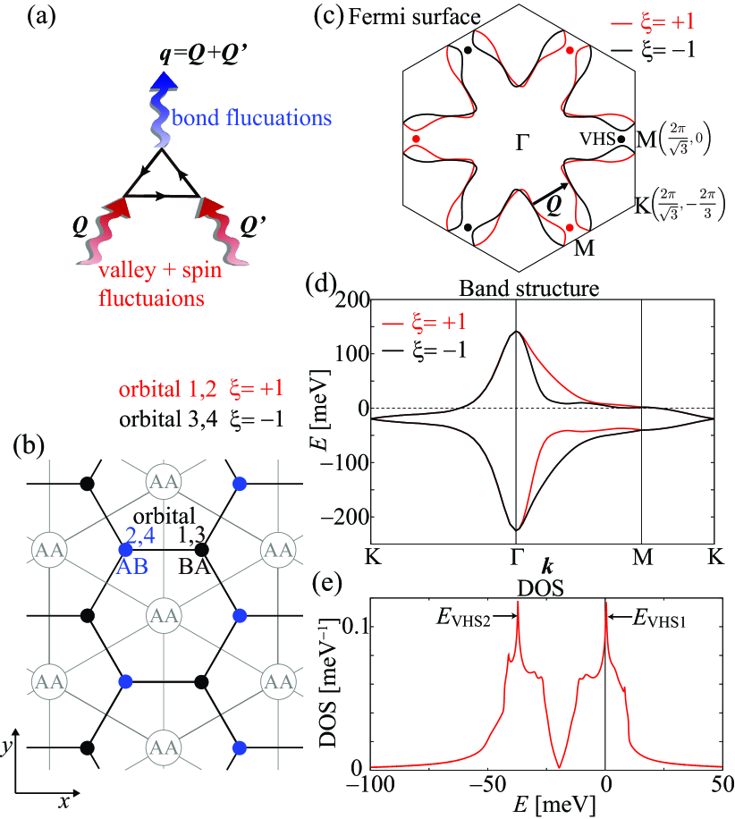
Figure 1: (a) Quantum interference between valley+spin fluctuations with the wavevector ${{\bm{Q}}}$ and ${{\bm{Q}}}^{\prime}$, which induces the bond fluctuations with $\bm{q}={{\bm{Q}}}+{{\bm{Q}}}^{\prime}$. (b) Moiré superlattice spanned by the AA spots. Wannier orbitals 1, 3 and 2, 4 are centered at the BA (black dots) and AB (blue dots) spots, respectively. (c) FSs of MATBG for $n=2.0$, where red (black) lines and dots denote the valley and the VHS points for $\xi=+1$ $(-1)$, respectively. The vector $\bm{Q}$ is the nesting vector. (d) Band structure and (e) DOS for $n=2.0$, which has peaks at the two VHS energies $E_{\rm VHS1}$ and $E_{\rm VHS2}$.

Here, we study the electronic states at $n=2.0$, which is close to the VHS filling $(n_{\rm VHS}=2.07)$. Figure 1(c) shows the FSs of MATBG for $\xi=\pm 1$. The weights of two same-valley orbitals on each FS are almost the same. For each valley, there are three VHS points at $E_{\rm VHS1}\sim 0.5$ meV, which locate near the FS around the M points, as shown in Fig. 1(c). Figures 1(d) and (e) show the band structure with $\xi=\pm 1$ and the total DOS, respectively. Split of the two VHS energies $E_{\rm VHS1}-E_{\rm VHS2}\sim 50$meV corresponds to the effective bandwidth, which is consistent with the STM measurement [20].

We calculate the spin (charge) susceptibilities ${\hat{\chi}}^{s(c)}(q)$ for $q=({{\bm{q}}},{\omega}_{m}=2m\pi T)$ based on the RPA. Details of formulation are presented in SM A [55]. ${\hat{\chi}}^{s(c)}(q)\propto(1-{\alpha}_{s(c)})^{-1}$ is given by the spin (charge) Stoner factor ${\alpha}_{s(c)}$. ${\alpha}_{s(c)}=1$ corresponds to spin (charge)-ordered state. In the present study, ${\alpha}_{s}={\alpha}_{c}={\alpha}$ is satisfied due to the relation $U^{\prime}=U$ $(J=0)$ [42]. Hereafter, we set $T=1.5$ meV. We fix ${\alpha}=0.83$, which corresponds to moderately correlated region, by setting the solo model parameter $U=39$ $(42)$ meV for $n=2.0$ $(2.4)$.

Figure 2(a) shows the obtained spin susceptibility $\chi^{s}_{1,1;1,1}({{\bm{q}}},0)$, which shows broad maximum peak at the intra-orbital nesting ${{\bm{Q}}}$ around the VHS points. We stress that the valley susceptibility $\chi^{c}_{\rm valley}\equiv\chi^{c}_{1,1;1,1}-\chi^{c}_{1,1;3,3}$ is exactly the same as $\chi^{s}_{1,1;1,1}$, as the consequence of the (approximate) $SU(4)$ symmetry of the MATBG model, as we explain in SM B [55].

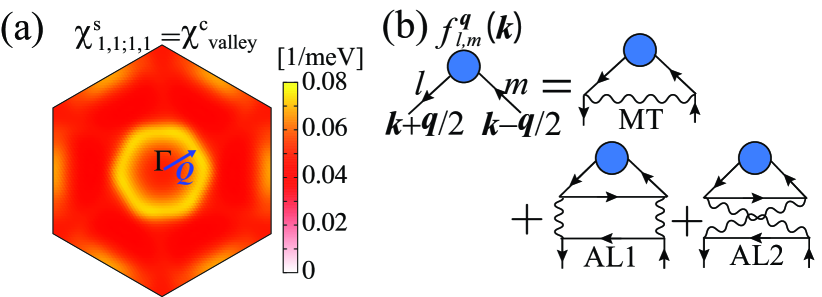
Figure 2: (a) ${{\bm{q}}}$ dependences of $\chi^{s}_{1,1;1,1}({{\bm{q}}},0)=\chi^{c}_{\rm valley}({{\bm{q}}},0)$ given by the RPA for $n=2.0$. (b) Feynman diagrams of the DW equation. Each wavy line represents valley+spin fluctuation-mediated interaction.

Hereafter, we derive the most strongest charge-channel density-wave (DW) instability, without assuming the order parameter and its wave vector. For this purpose, we use the DW equation method developed in Refs. [44, 46, 56]. The linearized DW equation is given as

$$\!\!\!\!\lambda_{{\bm{q}}}f^{{\bm{q}}}_{l,l^{\prime}}(k) = \frac{T}{N}\!\!\sum_{k^{\prime},m,m^{\prime}}{K}^{c,\bm{q}}_{l,l^{\prime};m,m^{\prime}}(k,k^{\prime})f^{{\bm{q}}}_{m,m^{\prime}}(k^{\prime}),$$ (2)

where the kernel function is $K^{c,\bm{q}}_{l,l^{\prime};m,m^{\prime}}(k,k^{\prime})=-\sum_{m_{1},m_{2}}\!I^{c,\bm{q}}_{l,l^{\prime};m_{1},m_{2}}(k,k^{\prime})G_{m_{1},m}\left(k^{\prime}+\frac{\bm{q}}{2}\right)\!G_{m^{\prime},m_{2}}(k^{\prime}-\frac{{{\bm{q}}}}{2})$. $\hat{I}^{c,\bm{q}}(k,k^{\prime})$ is the charge-channel irreducible interaction. $\lambda_{{\bm{q}}}$ is the eigenvalue of the form factor $\hat{f}^{{\bm{q}}}$, which represents the symmetry breaking in the self-energy, or equivalently, symmetry-breaking particle-hole pairing condensation. To satisfy the conservation laws [57, 58], one has to set $\hat{I}^{c,{{\bm{q}}}=\bm{0}}(k,k^{\prime})={\delta^{2}\Phi}/{\delta\hat{G}(k)\delta\hat{G}(k^{\prime})}$, where $\Phi$ is the Luttinger-Ward function. Here, we apply the one-loop approximation for $\Phi$, and the derived $\hat{I}^{c,\bm{q}}(k,k^{\prime})$ is given in SM A [55]. The charge-channel DW with wavevector ${{\bm{q}}}$ is established when the largest $\lambda_{{\bm{q}}}=1$. The charge-channel DW susceptibility is proportional to $(1-\lambda_{{\bm{q}}})^{-1}$. Therefore, $\lambda_{{\bm{q}}}$ represents the strength of the DW instability. The Maki–Thompson (MT) terms and Aslamazov–Larkin (AL) terms shown in Fig. 2(b) are included in the kernel function. The AL term is magnified by the convolution of spin/charge susceptibilities. In a simple single-orbital model, for example, the charge- and spin-channel AL terms are proportional to $C^{c}(q)\sim 3C^{s,s}(q)+C^{c,c}(q)$ and $C^{s}(q)\sim 2C^{s,c}(q)$, respectively, where $C^{a,b}(q)=\sum_{p}\chi^{a}(p)\chi^{b}(-p+q)$ and $a,b=c$ or $s$. Apparently, $C^{c(s)}(q)$ takes the largest value at ${{\bm{q}}}=\bm{0}$. (i.e., ${{\bm{Q}}}=-{{\bm{Q}}}^{\prime}$ in Fig. 1(a).) Therefore, the quantum interference mechanism by the AL terms causes novel DW orders at ${{\bm{q}}}=\bm{0}$ in various Hubbard models [43, 44, 45, 46, 51], and this mechanism will be significant for MATBG.

Figure 3(a) shows the ${{\bm{q}}}$ dependences of the obtained $\lambda_{{\bm{q}}}$ for the $C_{3}$ symmetry breaking $E$-symmetry and $C_{3}$ $A$-symmetry. Importantly, the ferro-nematic order is realized $(\lambda_{\bm{0}}=1)$ even when the SDW/CDW susceptibilities are small $(\alpha\ll 1)$ in the present theory. Figure 3(b) shows the dominant static form factor $f^{\bm{0}}_{1,1}({{\bm{k}}})$, which is derived from the analytic continuation of $\hat{f}^{{{\bm{q}}}}(k)$. The obtained form factor has no inter-valley component, and satisfies the time-reversal invariance. The obtained $\hat{f}^{\bm{0}}({{\bm{k}}})$ belongs to the two-dimensional $E$ representation, and its partner $\hat{f}^{\prime\bm{0}}({{\bm{k}}})$ is shown in SM C [55]. Thus, the direction of nematicity can be rotated by making the linear combination of $\hat{f}^{\bm{0}}({{\bm{k}}})$ and $\hat{f}^{\prime\bm{0}}({{\bm{k}}})$, it will be fixed by the anharmonic phonons and/or the fourth-order terms in the Ginzburg-Landau free energy.

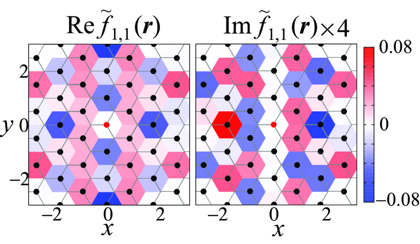
Figure S3: Re$\tilde{f}_{1,1}(\bm{r})$ and Im$\tilde{f}_{1,1}(\bm{r})$ of the form factor. Centers of orbital 1 (BA sites) are represented by black dots, and origins of $\bm{r}$ are shown by the red dots. Color maps show value at the black dots.

The obtained nematic state is mainly even parity as recognized in Fig. 3(b). However, sizable odd-parity component is mixed due to absence of the inversion symmetry. To show this, we examine the form factors in real space $\tilde{f}_{l,m}({{\bm{r}}})=\frac{1}{N}\sum_{{{\bm{k}}}}f^{\bm{0}}_{l,m}({{\bm{k}}})e^{i{{\bm{k}}}\cdot{{\bm{r}}}}$ shown in Fig. S3 in SM C [55]. Its real part Re$\tilde{f}_{1,1}({{\bm{r}}})$ has even parity, which gives the bond order ($=$ modulation of the correlated hopping integrals). On the other hand, its imaginary part Im$\tilde{f}_{1,1}({{\bm{r}}})$ has odd parity, which gives the valley current due to the time-reversal invariance [56, 59]. In the valley current state, the charge current in one valley is canceled by that in the opposite valley.

The ${{\bm{q}}}={{\bm{0}}}$ nematic order originates from the AL type quantum interference between the valley+spin fluctuations with ${{\bm{Q}}}\approx-{{\bm{Q}}}^{\prime}$ shown in Fig. 1(a). As we explain in SM B [55], the fifteen-channel valley+spin susceptibilities $\chi_{l}({{\bm{q}}})$ ($l=1\sim 15$) are equally enhanced, by reflecting the approximate $SU(4)$ symmetry of the model. Here, $l=1\sim 3$ for valley, $l=4\sim 6$ for spin, $l=7\sim 15$ for valley+spin composite channels. The interference among these $SU(4)$ valley+spin fluctuations [60] causes strong nematic criticality efficiently. In contrast, only spin fluctuations contribute in Fe-based superconductors with $J\gtrsim 0.1$ [43, 44, 45, 46, 47, 48, 49, 50] and cuprate superconductors with single orbital [51]. For this reason, the nematic order is more easily realized in MATBG.

The mechanism of the $E$-symmetry nematic order is clearly explained by focusing on the three VHS points on each valley as follows. The importance of the VHS in MATBG has been clarified in the RG studies [8, 26]. Figure 3(c) shows the intra-VHS attractive interaction $I>0$ and inter-VHS repulsive interaction $I^{\prime}<0$ driven mainly by the AL terms, as we describe in SM D 1 [55]. When the interaction is restricted for orbital 1, solved eigenvalues in the simple three VHS model are doubly degenerate $\lambda_{E}\propto I-I^{\prime}$ and non-degenerate $\lambda_{A}\propto I+2I^{\prime}$. The former $\lambda_{E}$ has degenerate form factors $(f_{A},f_{B},f_{C})\propto(1,1,-2)/\sqrt{6}$, $(1,-1,0)/\sqrt{2}$, where $f_{X}$ denotes the form factor at the VHS $X(=A,B,C)$ point. These form factors correspond to $E$-symmetry $f^{\bm{0}}_{1,1}$ in Fig. 3(b) and $f^{\prime\bm{0}}_{1,1}$ in SM C [55]. The latter $\lambda_{A}$ has $(f_{A},f_{B},f_{C})\propto(1,1,1)/\sqrt{3}$, which corresponds to the $A$-symmetry. Thus, dominant nematic $E$-symmetry with $\lambda_{E}(>\lambda_{A})$ is explained by the relations $I>0$ and $I^{\prime}<0$ derived by the valley+spin interference. This nematic state is robust independently of the shape of FSs once three VHS points exist in each valley.

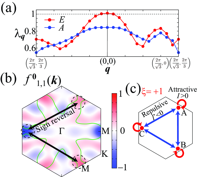
Figure 3: (a) Obtained ${{\bm{q}}}$ dependences of $\lambda_{{{\bm{q}}}}$ for the $E$ and $A$ symmetries for $n=2.0$. Maximum peak of $E$-symmetry at ${{\bm{q}}}={{\bm{0}}}$ means the emergence of the ferro nematic order. (b) Dominant form factor $f_{1,1}^{\bm{0}}({{\bm{k}}})$ in the Brillouin zone. The green lines indicate FSs for $\xi=+1$. The intra- (inter-) valley relation $f^{\bm{0}}_{1,1}({{\bm{k}}})=f^{\bm{0}}_{2,2}({{\bm{k}}})$ $(f^{\bm{0}}_{1,1}({{\bm{k}}})=f^{\bm{0}}_{3,3}(-{{\bm{k}}}))$ is satisfied. Black arrows show the sign-reversal between the VHS points. (c) Schematic picture of intra-VHS attractive $I_{\rm intra}>0$ and inter-VHS repulsive $I_{\rm inter}<0$ interactions for orbital $1$ in the simple three VHS model.

One of the main merit of the present bond-order theory is that the ferro (${{\bm{q}}}={{\bm{0}}}$) order is naturally obtained. Moreover, the present bond-order theory can cooperate with the phonon mechanism proposed in Ref. [24], as discussed in Ref. [61], while the phonon mechanism alone may give the bond order at ${{\bm{q}}}\approx{{\bm{Q}}}$. The nematic state was also discussed from the side of electron correlation by using the RG theory focusing on the VHS points [26]. The AL-type vertex correction (VC) are included in this theory [49, 50]. Therefore, the difference between the results of the present theory and those in Ref. [26] may originate from the difference of the theoretical models.

The present interference mechanism predicts that the nematic order in MATBG is established under very weak spin fluctuations, which is reminiscent of the nematicity without magnetism in FeSe [44, 45]. This result is very different from the vestigial nematic scenario under sufficiently long spin correlation length [32].

Here, we explain the robustness of the obtained nematic bond order, which is uniquely obtained near the VHS filling $(-0.3\lesssim n-n_{\rm VHS}\lesssim 0)$ in the present MATBG model. The nematic bond order also uniquely appears in the original MATBG model for $n\sim n_{\rm VHS}=0.7$ [53], as we demonstrate in SM D 2 [55]. Thus, the nematic bond order is robust in the case of $n\sim n_{\rm VHS}$, insensitively to the FS topology and position of the VHS points. This robustness is consistent with the intuitive explanation in Fig. 3(c) by focusing on the VHS points. Furthermore, the nematicity is stabilized by the relation $U=U^{\prime}$ $(J\ll U)$ in MATBG due to the contribution of the valley fluctuation interference; see SM E [55].

In the following, we explain the nematic ordered state. We denote $\Delta f$ as the maximum value of $|\hat{f}^{\bm{0}}({{\bm{k}}})|$. Figure 4 (a) shows FSs under the nematic order. We confirm that the $C_{3}$ symmetry is broken, and strong anisotropy appears along the $x$ axis, which is consistent with experiments [20, 21, 22, 23]. The DOS under the nematic order $\Delta f=5$ meV is shown in Fig. 4 (b). The energy of the VHS splits into $E_{\rm VHS1}^{\pm}\sim\pm\Delta f$ due to the ${{\bm{k}}}$ dependence of $\hat{f}^{\bm{0}}({{\bm{k}}})$. The dip structure in the DOS near the Fermi energy $E=0$ is consistent with STM measurement [20].

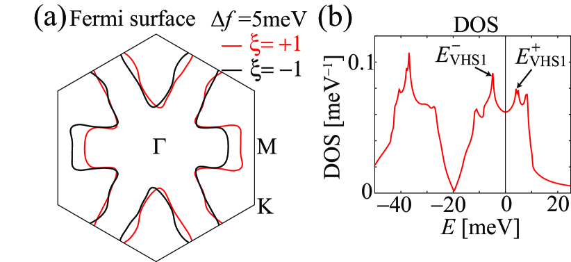
Figure 4: (a) FSs under the nematic order $\Delta f=5$ meV, where red (black) lines denote $\xi=+1(-1)$. (b) DOS for $\Delta f=5$ meV, where the VHS energy $E_{\rm VHS1}$ splits into $E_{\rm VHS1}^{\pm}\sim\pm\Delta f$.

Finally, we discuss the time-reversal-symmetry-broken order in the present theory at $n=2.4$. Figures 5(a) and (b) show the FSs and obtained form factor Re$f_{1,1}^{{{\bm{Q}}}_{1}}({{\bm{k}}})$, respectively. Here, the relation ${{\bm{Q}}}_{1}\sim 2{{\bm{Q}}}$ holds. The obtained $\hat{f}^{{{\bm{Q}}}_{1}}({{\bm{k}}})$ violates time-reversal-symmetry relation $f^{{{\bm{Q}}}_{1}}_{1,1}({{\bm{k}}})=f^{-{{\bm{Q}}}_{1}*}_{3,3}(-{{\bm{k}}})$, and brings the valley polarization. This state is caused by the cooperation among the inter-valley Hartree term and the AL type quantum interference with ${{\bm{Q}}}={{\bm{Q}}}^{\prime}$ in Fig. 1(a). ${{\bm{q}}}$ dependence of $\lambda_{{{\bm{q}}}}$ is shown in SM F [55]. The relation $U^{\prime}=U$ $(J=0)$ is important to realized the valley polarization.

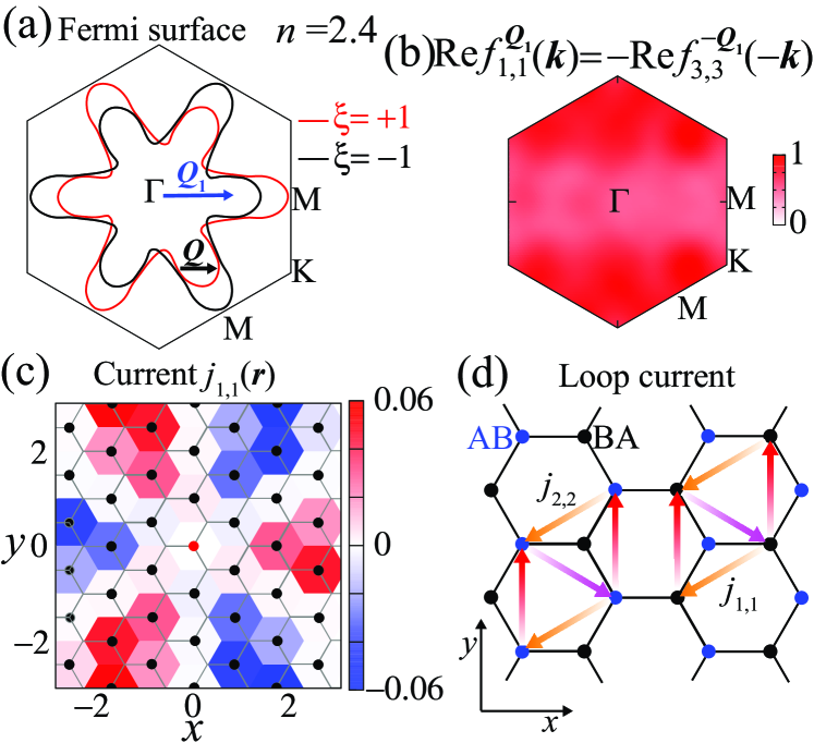
Figure 5: (a) FSs for $n=2.4$. (b) Obtained form factor $f_{1,1}^{\bm{Q}_{1}}({{\bm{k}}})$, which breaks the time reversal symmetry. The intra- (inter-) valley relation Re$f_{1,1}^{{{\bm{Q}}}_{1}}({{\bm{k}}})$ $={\rm Re}f_{2,2}^{{{\bm{Q}}}_{1}}({{\bm{k}}})$ (Re$f_{1,1}^{{{\bm{Q}}}_{1}}({{\bm{k}}})$ $=-{\rm Re}f_{3,3}^{-{{\bm{Q}}}_{1}}(-{{\bm{k}}})$) is satisfied. (c) $C_{3}$-symmetry current $j_{1,1}({{\bm{r}}})$ in the unit of $1$ meV/$\hbar$ without the form factor, where value at the BA spots (black dots) are depicted. Origin of ${{\bm{r}}}$ is represented by red dot. $j_{2,2}({{\bm{r}}})$ for the AB spots is the same as $j_{1,1}({{\bm{r}}})$ for the BA spots. (d) Schematic picture of the loop current $j_{1,1}$ and $j_{2,2}$ between the nearest intra-orbital sites. In the valley polarized state, the charge loop current emerges.

We stress that interesting charge loop current emerges in the valley polarized phase. In the absence of valley polarization, the current from the orbital $m$ at ${{\bm{r}}}^{\prime}$ to the orbital $l$ at ${{\bm{r}}}$ is given as $j_{l,m}({{\bm{r}}},{{\bm{r}}}^{\prime})=2{\rm Im}\langle\tilde{h}^{0}_{l,m}({{\bm{r}}},{{\bm{r}}}^{\prime})c^{\dagger}_{l}({{\bm{r}}})c_{m}({{\bm{r}}}^{\prime})\rangle_{0}$, where $\tilde{h}^{0}_{l,m}({{\bm{r}}},{{\bm{r}}}^{\prime})$ is the original hopping integral [56]. Figure 5(c) shows the current from the center site, $j_{1,1}({{\bm{r}}})\equiv j_{1,1}({{\bm{r}}},\bm{0})$ due to the imaginary hopping integrals in $\tilde{h}^{0}$. Figure 5 (d) shows a schematic intra-orbital current pattern. The direction of rotation in loop current $j_{1,1}$ is opposite to that in $j_{2,2}$. Because of the relation $j_{1,1}({{\bm{r}}})=-j_{3,3}({{\bm{r}}})$, the charge loop current is canceled, while pure valley loop current appears. In the presence of the valley polarization, the valley current is converted to the net charge loop current. The magnetic flux emerges in proportion to the valley polarization, and it will be measurable by several experimental methods.

In summary, we studied the origin of the nematic state in MATBG. We found that the ${{\bm{q}}}={{\bm{0}}}$ $C_{3}$-symmetry-breaking nematic state near the VHS filling is identified as the nematic bond order. This order originates from prominent quantum interference among moderate fluctuations of $SU(4)$ valley+spin composite operators. This nematicity is robust once three VHS points exist in each valley, insensitively to the shape of the FS. We also found the emergence of the time-reversal-symmetry-broken valley polarization, which accompanies the novel charge loop current. The present study revealed unexpected interesting similarities and differences between MATBG and Fe-based superconductors.

In SM G [55], we analyze the spin-channel DW equation [56], and it is verified that the spin-channel instability is not magnified by the spin-channel VCs. Thus, the charge-channel nematic bond order due to the charge-channel VCs is realized robustly. In addition, in SM H [55], we analyze the effect of the off-site Coulomb interactions $V_{n}$ included in the Kang-Vafek model [9]. It is verified that the nematic bond order driven by the valley + spin interference mechanism (in $U$-only model) is stabilized in the presence of $V_{n}$.

[Supplementary Material]
$SU(4)$ Valley + Spin Fluctuation Interference Mechanism for Nematic Order in Magic Angle Twisted Bilayer Graphene: Impact of Vertex Corrections

Seiichiro Onari and Hiroshi Kontani

Department of Physics, Nagoya University, Nagoya 464-8602, Japan

I.1 A: Model Hamiltonian of MATBG, formalism of the RPA and the DW equation

First, we introduce model for MATBG by referring the first-principles tight-binding model in Ref. [1]. However, in this original model, the VHS appears near $n\sim 0.7$, which is different from the experimentally observed $n_{\rm VHS}\sim 2$ [2]. Figure S1(a) shows the band structure of the original model for $n=0.5$, where all the hopping integrals are magnified $50$ times in order to fit the bandwidth observed by the STM measurement [2]. To shift the VHS filling to the experimental one, we reduce the magnitude of the imaginary part of second-nearest intra-orbital hopping 0.097 meV to 0.03 meV, while the real part is fixed. Also, we reduce the magnitude of the imaginary part of fourth-nearest intra-orbital hopping 0.039 meV to 0.02 meV. Finally, we magnify all the hopping integrals $50$ times. Figures S1(b), (c), and (d) show the band structure, the DOS, and $\chi^{c}_{1,1;1,1}({{\bm{q}}},0)$ in the obtained model, respectively. At $n=2.4$, the Fermi energy $(E=0)$ is above the energy of VHS. Although the band structure in the present model is similar to that in the original model, the energy difference between the valleys near the Fermi energy along $\Gamma$-M line increases in the present model.

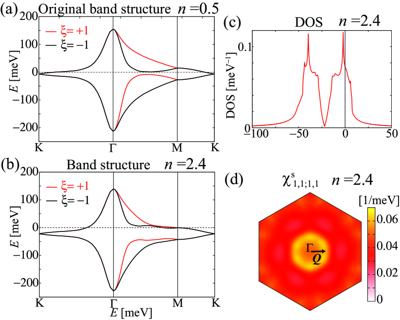
Figure S1: (a) Band structure in the original first-principles model for $n=0.5$, where red (black) lines denote valley $\xi=+1(-1)$. (b) Band structure in the present model for $n=2.4$. (c) DOS and (d) $\chi^{c}_{1,1;1,1}({{\bm{q}}},0)$ for $n=2.4$. Arrow $\bm{Q}$ denotes the nesting vector.

Here, we explain the Coulomb interaction in the orbital basis introduced in the present study. Only the Coulomb interactions between the orbitals with the same center position are taken into account. The Coulomb interactions for the spin and charge channels in the main text are generally given as

$$(\Gamma^{\mathrm{s}})_{l_{1},l_{2};l_{3},l_{4}}=\begin{cases}U,&l_{1}=l_{2}=l_{3}=l_{4}\\ U^{\prime},&l_{1}=l_{3}=l_{2}\pm 2=l_{4}\pm 2\\ J,&l_{1}=l_{2}=l_{3}\pm 2=l_{4}\pm 2\\ J,&l_{1}=l_{4}=l_{2}\pm 2=l_{3}\pm 2\\ 0,&\mathrm{otherwise},\end{cases}$$ (S1)

$$({\hat{\Gamma}}^{\mathrm{c}})_{l_{1},l_{2};l_{3},l_{4}}=\begin{cases}-U,&l_{1}=l_{2}=l_{3}=l_{4}\\ U^{\prime}-2J,&l_{1}=l_{3}=l_{2}\pm 2=l_{4}\pm 2\\ -2U^{\prime}+J,&l_{1}=l_{2}=l_{3}\pm 2=l_{4}\pm 2\\ -J,&l_{1}=l_{4}=l_{2}\pm 2=l_{3}\pm 2\\ 0.&\mathrm{otherwise}.\end{cases}$$ (S2)

Hamiltonian of the Coulomb interaction is given as

$$H^{\prime}=-\!\!\!\!\sum_{{{\bm{k}}}\bm{k^{\prime}}{{\bm{q}}},\sigma\sigma^{\prime}}\sum_{l_{1}l_{2}l_{3}l_{4}} \left(\frac{\Gamma^{c}+\Gamma^{s}\sigma\sigma^{\prime}}{4}\right)_{l_{1},l_{2};l_{3},l_{4}}$$ (S3)

$$\times c^{l_{1}\dagger}_{{{\bm{k}}}+{{\bm{q}}},\sigma}c^{l_{2}}_{{{\bm{k}}},\sigma}c^{l_{3}\dagger}_{\bm{k^{\prime}}-{{\bm{q}}},\sigma^{\prime}}c^{l_{4}}_{\bm{k^{\prime}},\sigma^{\prime}},$$

where $\sigma,\sigma^{\prime}=\pm 1$ denote spin.

We set $U^{\prime}=U$ and $J=0$ in the present study, since these relations are verified when only the Coulomb interactions between the orbitals with the same center position are taken into account[1, 3]. First, the relation $U^{\prime}=U$ is verified by the fact that the density of orbital 1(2) is the same as that of orbital 3(4) since the wave function of orbital 1(2) is identical to the complex conjugate wave function of orbital 3(4). Next, the inter-valley exchange interaction $J/U\ll 1$ has been explained in Ref. [1], where the integration in the calculation of the exchange interaction becomes very small due to the strongly oscillating phase. Moreover, the relation $J/U<10^{-3}$ has been confirmed in Ref. [3]. The effect of the inter-site Coulomb interaction is discussed in SM H.

By using the multiorbital Coulomb interaction, the spin (charge) susceptibility in the RPA is given by

$${\hat{\chi}}^{s(c)}(q)={\hat{\chi}^{0}}(q)[1-{\hat{\Gamma}}^{s(c)}{\hat{\chi}^{0}(q)}]^{-1},$$ (S4)

where the irreducible susceptibility is

$$\chi^{0}_{l,l^{\prime};m,m^{\prime}}(q)=-\frac{T}{N}\sum_{k}G_{l,m}(k+q)G_{m^{\prime},l^{\prime}}(k).$$ (S5)

${\hat{G}}(k)$ is the multiorbital Green function without self-energy ${\hat{G}}(k)=[(i{\epsilon}_{n}+\mu){\hat{1}}-{\hat{h}}^{0}({{\bm{k}}})]^{-1}$ for $k=[{{\bm{k}}},{\epsilon}_{n}=(2n+1)\pi T]$. Here, ${\hat{h}}^{0}({{\bm{k}}})$ is the matrix expression of $H^{0}$ and $\mu$ is the chemical potential.

The spin (charge) Stoner factor $\alpha_{s(c)}$ is defined as the maximum eigenvalue of $\hat{\Gamma}^{s(c)}\hat{\chi}^{0}(\bm{q},0)$. ${\alpha}_{c}={\alpha}_{s}={\alpha}$ is satisfied due to the relation $U^{\prime}=U$ $(J=0)$. In the present study, we fix ${\alpha}=0.83$ and $T=1.5$ meV, by setting $U=39$ $(42)$ meV for $n=2.0$ $(2.4)$. ($U$ is the solo parameter in the present study.) We use $N=72\times 72$ ${{\bm{k}}}$ meshes and $512$ Matsubara frequencies.

The charge-channel irreducible interaction $\hat{I}^{c,\bm{q}}(k,k^{\prime})$ in the DW equation (2) [4, 5] is given by

$$I^{c,\bm{q}}_{l,l^{\prime};m,m^{\prime}}(k,k^{\prime})=\sum_{b=s,c}\left[-\frac{a^{b}}{2}V^{b}_{l,m;l^{\prime},m^{\prime}}(k-k^{\prime})\right.$$

$$+\frac{T}{N}\!\!\sum_{p,l_{1},l_{2},m_{1},m_{2}}\!\!\!\!\!\!\!\!\!\!\frac{a^{b}}{2}V^{b}_{l,l_{1};m,m_{2}}\left(p+\frac{{{\bm{q}}}}{2}\right)V^{b}_{m_{1},l^{\prime};l_{2},m^{\prime}}\left(-p+\frac{{{\bm{q}}}}{2}\right)$$

$$\qquad\qquad\times G_{l_{1},m_{1}}(k-p)G_{l_{2},m_{2}}(k^{\prime}-p)$$

$$+\frac{T}{N}\!\!\!\!\sum_{p,l_{1},l_{2},m_{1},m_{2}}\!\!\!\!\!\!\!\!\!\!\frac{a^{b}}{2}V^{b}_{l,l_{1};l_{2},m^{\prime}}\left(p+\frac{{{\bm{q}}}}{2}\right)V^{b}_{m_{1},l^{\prime};m,m_{2}}\left(-p+\frac{{{\bm{q}}}}{2}\right)$$

$$\qquad\qquad\left.\times G_{l_{1},m_{1}}(k-p)G_{l_{2},m_{2}}(k^{\prime}+p)\right],$$ (S6)

where $a^{s}=3$, $a^{c}=1$, $p=({{\bm{p}}},{\omega}_{l})$, and $\hat{V}^{s(c)}(q)=\hat{\Gamma}^{s(c)}+\hat{\Gamma}^{s(c)}\hat{\chi}^{s(c)}(q)\hat{\Gamma}^{s(c)}$. In the conserving approximation scheme[6, 7], $\hat{I}^{c,{{\bm{q}}}=\bm{0}}(k,k^{\prime})\equiv{\hat{I}}^{\uparrow\uparrow,{{\bm{q}}}=\bm{0}}+{\hat{I}}^{\uparrow\downarrow,{{\bm{q}}}=\bm{0}}$ is given by

$$I^{\sigma\sigma^{\prime},{{\bm{q}}}=\bm{0}}_{l,l^{\prime};m,m^{\prime}}(k,k^{\prime})=\frac{\delta^{2}\Phi}{\delta G^{\sigma}_{l^{\prime},l}(k)\delta G^{\sigma^{\prime}}_{m,m^{\prime}}(k^{\prime})},$$ (S7)

where $\Phi$ is the Luttinger-Ward function within the one-loop approximation, and $\sigma$ denotes spin. In Eq. (S6), the first line corresponds to the Maki-Thompson (MT) term, and the second and third lines give the AL1 and AL2 terms, respectively. The AL terms are enhanced by the fluctuation interference $\hat{\chi}^{s(c)}({{\bm{Q}}})\times\hat{\chi}^{s(c)}(\bm{Q^{\prime}})$ shown in Fig 1(a). Thus, ${{\bm{q}}}={{\bm{Q}}}+\bm{Q^{\prime}}=\bm{0}$ nematic bond order is due to fluctuation interference with $\bm{Q^{\prime}}=-{{\bm{Q}}}$. In the MT term, the first-order term with respect to ${\hat{\Gamma}}^{s,c}$ gives the Hartree–Fock (HF) term in the mean-field theory.

I.2 B: Fifteen-channel valley+spin fluctuations in the MATBG model

In the main text, we explained that the nematic bond order in MATBG originates from the valley+spin fluctuation interference mechanism. Here, we explain why the present mechanism gives rise to remarkable nematic instability in MATBG, even stronger than Fe-based and cuprate superconductors.

We introduce the Pauli matrices for the spin-channel ($\rho=\pm 1$) and the valley-channel ($\xi=\pm 1$), ${\hat{\sigma}}_{m}$ and ${\hat{\tau}}_{n}$, respectively. Here, $m,n=1,2,3$. Then, the on-site Coulomb interaction is expressed as [8]

$$H^{\prime} = \frac{U}{16}\sum_{i}\left[-\sum_{\mu,\nu}({\hat{O}}^{i}_{\mu,\nu})^{2}+4({\hat{O}}^{i}_{0,0})^{2}\right],$$ (S8)

$${\hat{O}}^{i}_{\mu,\nu} = \sum_{\rho,\xi}({\hat{\sigma}}_{\mu}{\hat{\tau}}_{\nu})_{\rho\xi,\rho^{\prime}\xi^{\prime}}c_{i\rho\xi}^{\dagger}c_{i\rho^{\prime}\xi^{\prime}},$$ (S9)

where $\mu,\nu=0\sim 3$, $i$ is site index, and ${\hat{\sigma}}_{0}$ (${\hat{\tau}}_{0}$) is the identity matrix for spin (valley) sector. The Coulomb interaction $H^{\prime}$ in Eq. (S8) apparently possesses $SU(4)$ symmetry.

Next, we study the susceptibility with respect to the spin-valley operator ${\hat{O}}_{\mu,\nu}$ in Eq. (S9):

$$\chi_{\mu,\nu}({{\bm{q}}})=\frac{1}{2}\int_{0}^{\beta}du\langle T_{u}{\hat{O}}_{\mu,\nu}({{\bm{q}}},u){\hat{O}}_{\mu,\nu}(-{{\bm{q}}},0)\rangle,$$ (S10)

$${\hat{O}}_{\mu,\nu}({{\bm{q}}})=\sum_{{{\bm{k}}},a}({\hat{\sigma}}_{\mu}{\hat{\tau}}_{\nu})_{\rho\xi,\rho^{\prime}\xi^{\prime}}c_{{{\bm{k}}},a\rho\xi}^{\dagger}c_{{{\bm{k}}}+{{\bm{q}}},a^{\prime}\rho^{\prime}\xi^{\prime}}.$$ (S11)

Here, $a=$AB or BA in Fig. 1 (b), and $u$ is the imaginary time. Here, $\chi_{m,0}$ and $\chi_{0,n}$ are the spin and valley susceptibilities, respectively. Also, $\chi_{m,n}$ represent the susceptibility of the “spin-valley quadrupole order”, composed of the products of spin and pseudospin (= valley) operators.

Figure S2 represents the fifteen susceptibilities $\chi_{\mu,\nu}({{\bm{q}}})$ ($(\mu,\nu)\neq(0,0)$) given by the RPA in the MATBG model. By reflecting the $SU(4)$ symmetric Coulomb interaction in Eq. (S8), all $\chi_{\mu,\nu}({{\bm{q}}})$ take very similar values: Seven components with $(\mu,\nu)=(m,0),(\mu,3)$ are equivalent, and eight components with $(\mu,\nu)=(\mu,1),(\mu,2)$ are also equivalent. Thus, following relations are exact,

$$\chi_{m,0}({{\bm{q}}}) = \chi_{\mu,3}({{\bm{q}}})=\chi^{(1)}({{\bm{q}}})\quad{\rm for\,\,any}\,m\,{\rm and}\,\mu,$$

$$\chi_{\mu,1}({{\bm{q}}}) = \chi_{\nu,2}({{\bm{q}}})=\chi^{(2)}({{\bm{q}}})\quad{\rm for\,\,any}\,\mu\,{\rm and}\,\nu,$$ (S12)

where $\chi^{(1)}({{\bm{q}}})\sim\chi^{(2)}({{\bm{q}}})$ in the present MATBG model are shown in Fig. S2. These approximate fifteen-fold eigenstates with the form factors $f_{\mu\nu}\approx{\hat{\sigma}}_{\mu}{\hat{\tau}}_{\nu}$ are also obtained by the DW equation analysis. However, they do not correspond to the largest eigenvalue. The largest eigenvalue in the DW equation is the charge-channel bond-order state with $E$-symmetry, ${\bm{f}}_{\rm bond}\approx{\hat{\sigma}}_{0}{\hat{\tau}}_{0}(f^{\bm{0}}({{\bm{k}}}),f^{\prime\bm{0}}({{\bm{k}}}))$, as we derived in the main text. The eigenvalue of this bond-order state is strongly magnified by the AL-type VCs in the DW equation.

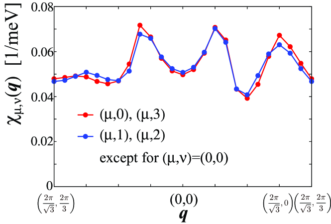
Figure S2: $\chi_{\mu,\nu}({{\bm{q}}})$ in the present MATBG model given by the RPA.

Now, we consider the main driving force of the nematic order. The AL terms in Fig. 2 (b) are composed of the convolutions of $\chi_{\mu,\nu}({{\bm{q}}})$. Because fifteen susceptibilities in Fig. S2 exhibit similar ${{\bm{q}}}$-dependences, the ratio of the contributions from the spin ($\chi_{m,0}({{\bm{q}}})$), the valley ($\chi_{0,n}({{\bm{q}}})$), and the quadrupole ($\chi_{m,n}({{\bm{q}}})$) susceptibilities to the AL terms are approximately $\frac{3}{15}$ : $\frac{3}{15}$ : $\frac{9}{15}$. Therefore, the AL interference process is caused by not only independent spin and valley fluctuations, but also spin+valley composite (quadrupole) fluctuations.

I.3 C: Parity mixing in form factor

Here, we explain the real-space structure of the obtained ${{\bm{q}}}={{\bm{0}}}$ form factor in MATBG. Figure S4 shows real part of Fourier transformed form factor Re$\tilde{f}_{1,1}({{\bm{r}}})$ and imaginary part of that Im$\tilde{f}_{1,1}({{\bm{r}}})$. Re$\tilde{f}_{1,1}({{\bm{r}}})$ is even parity, and it gives the bond order between the position ${{\bm{0}}}$ and ${{\bm{r}}}$. On the other hand, Im$\tilde{f}_{1,1}({{\bm{r}}})$ has odd parity. Thus, parity mixing in the form factor is confirmed in MATBG, and it gives the time-reversal-invariant valley current order [9]. Thus, both even-parity and odd-parity components coexist in the present order parameter. This “parity mixing order” is a natural consequence of the violation of the inversion symmetry in MATBG: The primary even-parity component in $f$ induces sizable secondary odd-parity one through the imaginary intra-orbital hopping integrals due to the inversion symmetry breaking.

Figure S4 shows the off-diagonal form factor $f^{{\bm{0}}}_{1,2}({{\bm{k}}})$, which is slightly smaller than the diagonal form factor. This form factor is invariant under the time reversal operation $f^{{\bm{0}}}_{1,2}({{\bm{k}}})=f^{{{\bm{0}}}*}_{3,4}(-{{\bm{k}}})$. Even parity Re$\tilde{f}_{1,2}({{\bm{r}}})(=$Re$\tilde{f}_{2,1}(-{{\bm{r}}}))$ is also mixed by odd parity Im$\tilde{f}_{1,2}({{\bm{r}}})(=-$Im$\tilde{f}_{2,1}(-{{\bm{r}}}))$.

Since the obtained form factors belong to the two-dimensional $E$ representation, the other form factors $\hat{f}^{\prime{{\bm{0}}}}$ shown in Fig. S5 has the same eigenvalue $\lambda_{{\bm{0}}}$. The direction of anisotropy of $f^{\prime\bm{0}}$ is different from that of $f^{\bm{0}}$ shown in the main text. Thus, we can rotate the direction of anisotropy by making the linear combination of $\hat{f}^{{{\bm{0}}}}$ and $\hat{f}^{\prime{{\bm{0}}}}$. In real systems, the direction of nematicity will be fixed by the anharmonic phonons and/or the fourth-order terms in the Ginzburg-Landau free energy.

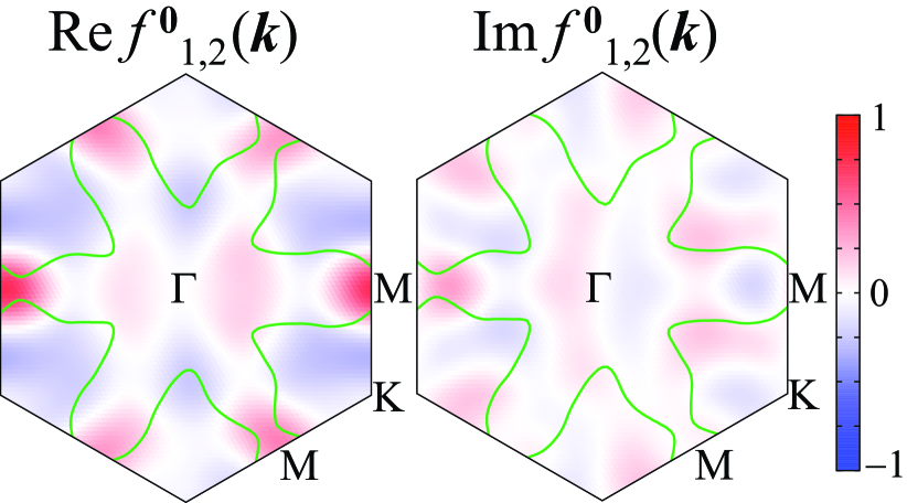
Figure S4: Off-diagonal form factor explained in the main text for $n=2.0$ The green lines indicate FSs for $\xi=+1$.

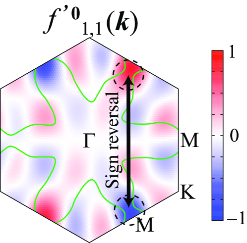
Figure S5: Degenerate form factor $f^{\prime{{\bm{0}}}}({{\bm{k}}})$ for $n=2.0$. The green lines and black arrow indicates FSs for $\xi=+1$ and sign-reversal between the VHS points.

I.4 D: Robustness of nematic order and impact of three VHS points

I.4.1 1. Analytic discussion on a simple three VHS model

First, we explain an origin of strong intra- and inter-VHS interactions due to the VCs in the DW Eq. (2) in MATBG. The derived interaction originates from the fluctuation interference mechanism, and it naturally promotes the nematicity in $E$-symmetry.

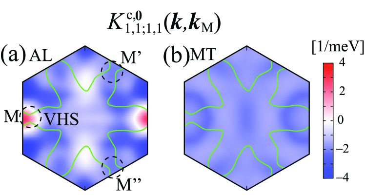
Figure S6: (a) $\bm{k}$ dependences of kernel $K^{c,\bm{0}}_{1,1;1,1}({{\bm{k}}},{{\bm{k}}}_{M})$ for the AL terms and (b) that for the MT term, composed of orbital $1$. Here, ${{\bm{k}}}_{M}=(-\frac{2\pi}{\sqrt{3}},0)$, ${{\bm{k}}}_{M^{\prime}}=(\frac{\pi}{\sqrt{3}},\pi)$, and ${{\bm{k}}}_{M^{\prime\prime}}=(\frac{\pi}{\sqrt{3}},-\pi)$.

Figures S6(a) and (b) show $\bm{k}$ dependences of kernel $K^{c,\bm{0}}_{1,1;1,1}({{\bm{k}}},\bm{k}_{M})$ for the AL and MT terms composed of the orbital 1 in valley $\xi=+1$, where ${{\bm{k}}}_{M}=(-\frac{2\pi}{\sqrt{3}},0)$ at the M point. The obtained kernel takes sizable positive value at ${{\bm{k}}}\sim{{\bm{k}}}_{M}$, while it exhibits negative values at ${{\bm{k}}}\sim{{\bm{k}}}_{M^{\prime}}$ and ${{\bm{k}}}_{M^{\prime\prime}}$. The ${{\bm{k}}}$ dependence of $K^{c,\bm{0}}_{1,1;1,1}({{\bm{k}}},\bm{k}_{M})$ favors the $E$-symmetry nematicity. In the following, we explain that $\bm{k}$ dependence of $K^{c,\bm{0}}_{1,1;1,1}({{\bm{k}}},\bm{k}_{M})$ is mainly caused by the AL1 term. We note that $K^{c,\bm{0}}({{\bm{k}}},\bm{k^{\prime}})$ is proportional to $I^{c,\bm{0}}({{\bm{k}}},\bm{k^{\prime}})$.

As we discussed in Ref. [5], the $k$, $k^{\prime}$ dependence of AL1 term is mainly determined by the momentum dependence of the particle-hole (p-h) propagator, rather than $q$ dependence of $\chi^{s(c)}(q)$. The p-h propagator is given as

$$\phi_{\mbox{p-h}}({{\bm{q}}},{\omega}_{m})\equiv$$

$$\frac{T}{N}\displaystyle\sum_{{{\bm{p}}},{\omega}_{l}}G_{1,1}({{\bm{q}}}+{{\bm{p}}},{\omega}_{m}+{\omega}_{l})G_{1,1}({{\bm{p}}},{\omega}_{l})$$

$$\times\theta({\omega}_{c}-|{\omega}_{m}+{\omega}_{l}|)\theta({\omega}_{c}-|{\omega}_{l}|),$$ (S13)

and the AL1 term in $I^{c,\bm{0}}(k,k^{\prime})$ in Eq. (S6) is proportional to $\phi_{\mbox{p-h}}(k-k^{\prime})$ since ${{\bm{q}}}$ dependence of $\chi^{s(c)}(q)$ is moderate in MATBG. The cutoff energy ${\omega}_{c}\ll E_{\rm F}$ is related to energy-scale of spin (valley) fluctuations ${\hat{\chi}}^{s(c)}$ in $\hat{V}^{s(c)}$ in AL1 term. Feynman diagram of $\phi_{\mbox{p-h}}(q)$ is shown in Fig. S7(a).

Since the energy scale ${\omega}_{s}$ of ${\hat{\chi}}^{s(c)}(q)$ satisfies ${\omega}_{s}\lesssim 2\pi T$ in the moderately correlated MATBG, the relation $\pi T<{\omega}_{c}<3\pi T$ in Eq. (S13) is reasonable. For simplicity, we apply the lowest Matsubara approximation for the kernel function as $I^{c,\bm{0}}({{\bm{k}}},\pi T,\bm{k^{\prime}},\pi T)+I^{c,\bm{0}}({{\bm{k}}},\pi T,\bm{k^{\prime}},-\pi T)$, which is proportional to

$$\tilde{\phi}_{\mbox{p-h}}({{\bm{q}}})\equiv{\phi}_{\mbox{p-h}}({{\bm{q}}},0)+{\phi}_{\mbox{p-h}}({{\bm{q}}},2\pi T).$$ (S14)

Figure S7(b) shows the obtained $\tilde{\phi}_{\mbox{p-h}}({{\bm{k}}}-{{\bm{k}}}_{M})$ as a function of ${{\bm{k}}}$. We see that $\tilde{\phi}_{\mbox{p-h}}({{\bm{k}}}-{{\bm{k}}}_{M})$ well reproduces the result for the AL terms in Fig. S6(a).

Hereafter, we explain an origin of the ${{\bm{q}}}$ dependence of $\tilde{\phi}_{\mbox{p-h}}({{\bm{q}}})$. It is approximately given as

$$\!\!\!\!\tilde{\phi}_{\mbox{p-h}}({{\bm{q}}}) \sim \frac{T}{N}\sum_{\bm{p}}\frac{2\varepsilon_{{{\bm{q}}}+\bm{p}}\varepsilon_{{{\bm{p}}}}}{[(\pi T)^{2}+\varepsilon_{{{\bm{q}}}+\bm{p}}^{2}][(\pi T)^{2}+\varepsilon_{\bm{p}}^{2}]},$$ (S15)

where $\varepsilon_{{{\bm{k}}}}=h^{0}_{1,1}({{\bm{k}}})-\mu$. Thus, $\tilde{\phi}_{\mbox{p-h}}({{\bm{q}}})$ exhibits sizable positive value for ${{\bm{q}}}=\bm{0}$, while it becomes small in magnitude and can be negative for finite $|{{\bm{q}}}|$ due to the cancellation of $\varepsilon_{{{\bm{q}}}+\bm{p}}\varepsilon_{{{\bm{p}}}}$ in the numerator of Eq. (S15).

The AL1 term $I^{c,\bm{0}}(k,k^{\prime})$ is proportional to $\tilde{\phi}_{\mbox{p-h}}({{\bm{k}}}-\bm{k^{\prime}})$, and it is enhanced by the convolution of valley+spin susceptibilities at low temperatures [5]. In addition, as shown in Fig. S6(b), the MT term $(\propto-V^{s}_{1,1;1,1}(k-k^{\prime}))$ gives negative interaction.

We stress that $\tilde{\phi}_{\mbox{p-h}}({{\bm{q}}})$ becomes always negative if we set ${\omega}_{c}\sim E_{F}$. In fact, $\tilde{\phi}_{\mbox{p-h}}(q)=-\chi^{0}({{\bm{q}}},0)-\chi^{0}({{\bm{q}}},2\pi T)$ for ${\omega}_{c}=\infty$. Therefore, the relation ${\omega}_{c}\ll E_{F}$ is important to obtain the nematic order.

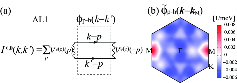
Figure S7: (a)Feynman diagram of $\phi_{\mbox{p-h}}(k-k^{\prime})$ in $I^{c,\bm{0}}(k,k^{\prime})$ of the AL1 term. (b)$\bm{k}$ dependence of $\tilde{\phi}_{\mbox{p-h}}({{\bm{k}}}-\bm{k}_{M})$ for cutoff $\pi T<{\omega}_{c}<3\pi T$. Positive peak appears at ${{\bm{k}}}=\bm{k}_{M}$.

Next, we clarify that the $E$-symmetry nematicity is caused by the intra-VHS interaction $I>0$ and inter-VHS one $I^{\prime}<0$ on the simple three VHS model in the main text. In this model, ${{\bm{k}}}$ and $\bm{k^{\prime}}$ point are limited to the three VHS points $A$, $B$, and $C$ in Fig. 3(c). Thus, $I^{c,\bm{0}}_{1,1;1,1}({{\bm{k}}},\bm{k^{\prime}})$ in the DW Eq. is given by the following $3\times 3$ matrix,

$$\hat{I}^{c,\bm{0}}_{1,1;1,1}=\left(\begin{array}[]{ccc}I&I^{\prime}&I^{\prime}\\ I^{\prime}&I&I^{\prime}\\ I^{\prime}&I^{\prime}&I\end{array}\right).$$ (S16)

By using the DOS of orbital 1 at the Fermi energy $N_{0}$ and the form factors $\vec{f}=^{t}\!\!(f_{A},f_{B},f_{C})$, where $f_{X}$ denotes the form factor for orbital 1 at the VHS $X(=A,B,C)$ point, the DW equation in Eq. (2) is given as

$$\lambda_{\bm{0}}\vec{f}=N_{0}\hat{I}^{c,\bm{0}}_{1,1;1,1}\vec{f}.$$ (S17)

The solved eigenvalues are doubly degenerate $\lambda_{E}\propto I-I^{\prime}$ and non-degenerate $\lambda_{A}\propto I+2I^{\prime}$. The former $\lambda_{E}$ has degenerate form factor (eigenvector) $(f_{A},f_{B},f_{C})\propto(1,1,-2)/\sqrt{6}$, $(1,-1,0)/\sqrt{2}$. These form factors correspond to $E$-symmetry $f^{\bm{0}}_{1,1}$ in Fig. 3(b) and $f^{\prime\bm{0}}_{1,1}$ in SM C. The latter $\lambda_{A}$ has $(f_{A},f_{B},f_{C})\propto(1,1,1)/\sqrt{3}$, which corresponds to the $A$-symmetry order. Thus, the nematic $E$-symmetry with $\lambda_{E}(>\lambda_{A})$ is explained by the three VHS model due to the relations $I>0$ and $I^{\prime}<0$. The relation $I^{\prime}<0$ induces sign-reversal in form factors between the VHS points. The nematic order due to the valley+spin fluctuation interference is robust independently of the shape of FS and position of VHS point once three VHS points exist in each valley.

To summarize, we studied the charge-channel interaction in the DW Eq. (2), $I^{c,\bm{0}}$, beyond the mean-field approximation. Strong attractive intra-VHS interaction emerges due to the valley+spin fluctuation interference described by the AL processes. In addition, repulsive inter-VHS interaction originates from the AL + MT processes. These intra- and inter-VHS interactions naturally induce the $E$-symmetry nematicity in MATBG. The nematic order is robust once three VHS points exist in each valley.

I.4.2 2. Numerical study on the original first-principles MATBG model

In order to verify the robustness of the nematic bond order, we investigate the original first-principles model[1], by multiplying all the hopping integrals by $50$ in order to fit the bandwidth obtained by the STM measurement [2]. The FSs and band structure are shown in Figs. S8(a) and S1(a). We stress that the band structure is similar to Fig. 1(d) in the main text. In contrast, the FS structure is very different from Fig. 1(c) in the main text, and the VHS filling $n_{\rm VHS}=0.7$ is also very different from $n_{\rm VHS}=2.07$ in the main text. Moreover, the positions of the VHS points are different. These differences mainly come from the reduction of the imaginary intra-orbital hoppings.

Nonetheless of the large difference between two models, the nematic state is also obtained in the original first-principles model when the filling is slightly lower than $n_{\rm VHS}$. Figure S8(b) shows ${{\bm{q}}}$ dependences of the DW equation eigenvalue $\lambda_{{{\bm{q}}}}$ for the $E$-symmetry and $A$-symmetry for $n=0.5$ and ${\alpha}=0.91$ ($U=28.7$ meV) at $T=1.5$ meV. The obtained $\lambda_{{{\bm{q}}}}$ for $E$-symmetry is dominant and has peak at ${{\bm{q}}}={{\bm{0}}}$, which corresponds to the emergence of the ${{\bm{q}}}={{\bm{0}}}$ nematic order. The obtained doubly degenerate $E$-symmetry form factors $f^{\bm{0}}_{1,1}({{\bm{k}}})$ and $f^{\prime\bm{0}}_{1,1}({{\bm{k}}})$ shown in Fig. S8(c) are similar to those in Fig. 3(b) in the main text and Fig. S5. The real part Re$\tilde{f}_{1,1}({{\bm{r}}})$ gives the bond order, and the imaginary part Im$\tilde{f}_{1,1}({{\bm{r}}})$ gives the spontaneous current. Thus, the nematic state near the VHS filling is also identified as the nematic bond order based on the original model. The $E$-symmetry solution is doubly degenerate similarly to the results in the model in main text.

In summary, although the value of $n_{\rm VHS}$ and the FS structure are very different between the original first-principles model and the present model in the main text, both models lead to essentially the same nematic bond order solution. Thus, ${{\bm{q}}}={{\bm{0}}}$ nematic bond order is stably obtained near the VHS filling irrespective of huge difference in the FS structure. This result is verified by the analysis of the simple three VHS model in Fig 3(c) and SM D 1.

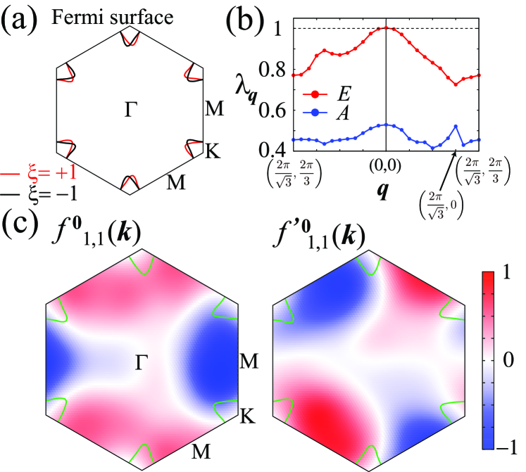
Figure S8: (a) FSs for $n=0.5$ in the original first-principles model, where red (black) lines denote the valley $\xi=+1$ $(-1)$. (b) Obtained ${{\bm{q}}}$ dependences of $\lambda_{{{\bm{q}}}}$ for the $E$-symmetry and $A$-symmetry for $n=0.5$ in the original model. (c) Doubly degenerate form factors $f_{1,1}^{\bm{0}}({{\bm{k}}})$ and $f^{\prime\bm{0}}_{1,1}({{\bm{k}}})$ in the Brillouin zone. The green lines indicate FSs for $\xi=+1$.

I.5 E: Numerical study for $J\neq 0$

Here, we show results for $J\neq 0$ and $U=U^{\prime}+2J$, which is satisfied in the rotationally invariant systems. In the case $J\neq 0$, $\alpha_{s}=\alpha_{c}$ is violated and $\alpha_{s}$ becomes larger than $\alpha_{c}$. Figure S9 shows $J/U$ dependences of the DW eigenvalue $\lambda_{\bm{0}}$ for the $E$ and $A$ symmetries for $n=2.0$ by fixing ${\alpha}_{s}=0.90$. It is robust for $J/U<0.1$ that the $E$-symmetry nematic bond ordered state dominates over the $A$-symmetry ordered state.

However, the value of $\lambda_{\bm{0}}$ is strongly suppressed for $J/U\gtrsim 0.03$ as shown by arrow in Fig. S9. This suppression is caused by the decreased valley fluctuation due to ${\alpha}_{s}>{\alpha}_{c}$ in finite $J$. Thus, $J=0$ and $U=U^{\prime}$ are important features in MATBG to realize the nematic bond ordered state.

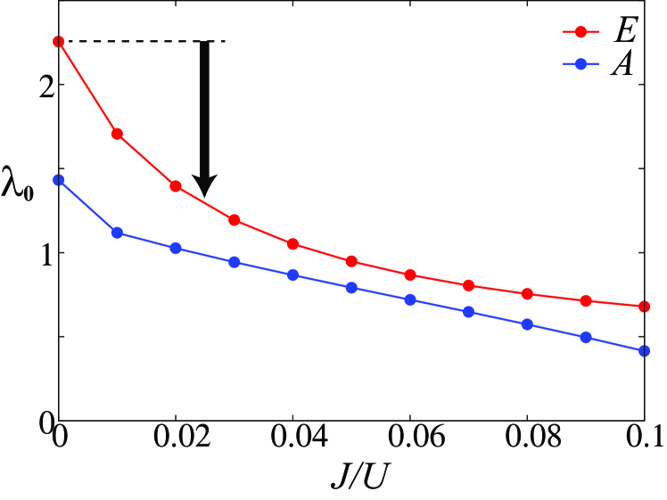
Figure S9: $J/U$ dependences of the DW eigenvalue $\lambda_{\bm{0}}$ for the $E$ and $A$ symmetries for $n=2.0$ and ${\alpha}_{s}=0.9$ at $T=1.5$meV. Black arrow shows strong suppression of $\lambda_{\bm{0}}$ for finite $J$.

I.6 F: ${{\bm{q}}}$ dependence of $\lambda_{{{\bm{q}}}}$ for $n=2.4$

We discuss the ${{\bm{q}}}$ dependence of $\lambda_{{{\bm{q}}}}$ for $n=2.4$. Figure S10 shows $\lambda_{{{\bm{q}}}}$ obtained by the model in the main text. The $\lambda_{{{\bm{q}}}}$ has peak at ${{\bm{q}}}={{\bm{Q}}}_{1}\sim 2{{\bm{Q}}}$ due to the quantum interference mechanism in Fig 1(a). The obtained form factor $\hat{f}^{{{\bm{q}}}}({{\bm{k}}})$ violates time-reversal-symmetry. $\hat{f}^{{{\bm{q}}}}({{\bm{k}}})$ satisfies relations Re$f_{1,1}^{{{\bm{q}}}}({{\bm{k}}})$ $={\rm Re}f_{2,2}^{{{\bm{q}}}}({{\bm{k}}})$ and Re$f_{1,1}^{{{\bm{q}}}}({{\bm{k}}})$ $=-{\rm Re}f_{3,3}^{-{{\bm{q}}}}(-{{\bm{k}}})$. ${{\bm{k}}}$ dependence of $\hat{f}^{{{\bm{q}}}}({{\bm{k}}})$ is small as shown in Fig. 5(b).

We confirm that $\lambda_{{{\bm{Q}}}_{1}}$ is enlarged by the Hartree term in the MT terms and the AL type quantum interference between the valley + spin fluctuations with ${{\bm{Q}}}={{\bm{Q}}}^{\prime}$.

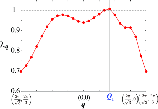
Figure S10: ${{\bm{q}}}$ dependence of $\lambda_{{{\bm{q}}}}$ for $n=2.4$.

I.7 G: Smallness of spin-channel DW instabilities in MATBG

In order to discuss the effect of the VCs for the spin-channel density waves, we analyze the spin-channel DW equation with spin-channel irreducible interaction, ${\hat{I}}^{s,{{\bm{q}}}=\bm{0}}\equiv{\hat{I}}^{\uparrow\uparrow,{{\bm{q}}}=\bm{0}}-{\hat{I}}^{\uparrow\downarrow,{{\bm{q}}}=\bm{0}}$, where ${\hat{I}}^{{\sigma}{\sigma}^{\prime},{{\bm{q}}}=\bm{0}}(k,k^{\prime})=\delta\Phi/\delta{\hat{G}}^{\sigma}(k)\delta{\hat{G}}^{{\sigma}^{\prime}}(k^{\prime})$. The DW equation is given as [9]

$$\eta_{{\bm{q}}}g^{{{\bm{q}}}}_{l,l^{\prime}}(k)=\frac{T}{N} \!\!\sum_{k^{\prime},m,m^{\prime}}{K}^{s,\bm{q}}_{l,l^{\prime};m,m^{\prime}}(k,k^{\prime})g^{{{\bm{q}}}}_{m,m^{\prime}}(k^{\prime}),$$ (S18)

$$K^{s,\bm{q}}_{l,l^{\prime};m,m^{\prime}}(k,k^{\prime})= -\sum_{m_{1},m_{2}}\!\!\!\!I^{s,\bm{q}}_{l,l^{\prime};m_{1},m_{2}}(k,k^{\prime})G_{m_{1},m}\left(k^{\prime}+\frac{\bm{q}}{2}\right)$$ (S19)

$$\times G_{m^{\prime},m_{2}}(k^{\prime}-\frac{{{\bm{q}}}}{2}),$$

where $\eta_{{{\bm{q}}}}$ and $\hat{g}^{{{\bm{q}}}}$ are the eigenvalue and the form factor of the spin-channel DW equation, respectively. The spin-channel $\hat{I}^{s,{{\bm{q}}}}$ is given as

$$\!\!\!I^{s,\bm{q}}_{l,l^{\prime};m,m^{\prime}}(k,k^{\prime})=\frac{1}{2}V^{s}_{l,m;l^{\prime},m^{\prime}}(k-k^{\prime})-\frac{1}{2}V^{c}_{l,m;l^{\prime},m^{\prime}}(k-k^{\prime})$$

$$+\frac{T}{N}\!\!\sum_{p,l_{1},l_{2},m_{1},m_{2}}\!\!\!\!\!\!\!\!\!\!\left[V^{s}_{l,l_{1};m,m_{2}}\left(p+\frac{{{\bm{q}}}}{2}\right)V^{s}_{m_{1},l^{\prime};l_{2},m^{\prime}}\left(-p+\frac{{{\bm{q}}}}{2}\right)\right.$$

$$\left.+\frac{1}{2}V^{s}_{l,l_{1};m,m_{2}}\left(p+\frac{{{\bm{q}}}}{2}\right)V^{c}_{m_{1},l^{\prime};l_{2},m^{\prime}}\left(-p+\frac{{{\bm{q}}}}{2}\right)\right.$$

$$\left.+\frac{1}{2}V^{c}_{l,l_{1};m,m_{2}}\left(p+\frac{{{\bm{q}}}}{2}\right)V^{s}_{m_{1},l^{\prime};l_{2},m^{\prime}}\left(-p+\frac{{{\bm{q}}}}{2}\right)\right]$$

$$\times G_{l_{1},m_{1}}(k-p)G_{l_{2},m_{2}}(k^{\prime}-p)$$

$$+\frac{T}{N}\!\!\sum_{p,l_{1},l_{2},m_{1},m_{2}}\!\!\!\!\!\!\!\!\!\!\left[-V^{s}_{l,l_{1};l_{2},m^{\prime}}\left(p+\frac{{{\bm{q}}}}{2}\right)V^{s}_{m_{1},l^{\prime};m,m_{2}}\left(-p+\frac{{{\bm{q}}}}{2}\right)\right.$$

$$+\frac{1}{2}V^{s}_{l,l_{1};l_{2},m^{\prime}}\left(p+\frac{{{\bm{q}}}}{2}\right)V^{c}_{m_{1},l^{\prime};m,m_{2}}\left(-p+\frac{{{\bm{q}}}}{2}\right)$$

$$\left.+\frac{1}{2}V^{c}_{l,l_{1};l_{2},m^{\prime}}\left(p+\frac{{{\bm{q}}}}{2}\right)V^{s}_{m_{1},l^{\prime};m,m_{2}}\left(-p+\frac{{{\bm{q}}}}{2}\right)\right]$$

$$\times G_{l_{1},m_{1}}(k-p)G_{l_{2},m_{2}}(k^{\prime}+p).$$ (S20)

Figure S11(a) displays ${{\bm{q}}}$ dependence of the obtained spin-channel eigenvalue $\eta_{{{\bm{q}}}}$, together with $\alpha({{\bm{q}}})$ and the charge-channel eigenvalue $\lambda_{{{\bm{q}}}}$ for $E$-symmetry shown in Fig. 3(a). Here, $\alpha({{\bm{q}}})$ is the RPA Stoner factor at fixed ${{\bm{q}}}$. Note that $\alpha=\max_{{\bm{q}}}\alpha({{\bm{q}}})$. We find the relation $\eta_{{{\bm{q}}}}\sim{\alpha}({{\bm{q}}})\sim 0.8$, and the obtained spin-channel form factor $g^{{{\bm{q}}}={\bm{0}}}_{l,m}(k)$ is nearly $k$-independent. Because $\chi^{s}({{\bm{q}}})\propto 1/(1-\eta_{{{\bm{q}}}})$ is very similar to $\chi^{{\rm RPA},s}({{\bm{q}}})\propto 1/(1-{\alpha}({{\bm{q}}}))$, the VCs for the spin-channel density-waves are unimportant. Therefore, the obtained nematic bond order is robust even when both charge-channel and spin-channel VCs are taken into account.

Now, we explain the reason why the AL terms induce strong $O_{0,0}$-channel instability, based on the $O_{\mu,\nu}$-channel decomposition of the Coulomb interaction in Eq. (S8) by following Ref. [8]. The three-point vertex in the AL term $\Lambda^{({\alpha},{\beta})}_{(\mu,\nu),(\mu^{\prime},\nu^{\prime})}$ is shown in Fig. S11(b), where $f(k)O_{{\alpha},{\beta}}$ is the DW form factor and $UO_{\mu,\nu}$ ($UO_{\mu^{\prime},\nu^{\prime}}$) represents the decomposed Coulomb interaction in Eq. (S8). $O_{\mu,\nu}$ is converted to the $SU(4)$ valley + spin susceptibility $\chi_{\mu,\nu}$ after taking the average. The three-point vertex represent the coupling constant between the DW form factor and the $SU(4)$ valley + spin susceptibilities in the interference mechanism. The relation $\Lambda^{({\alpha},{\beta})}_{(\mu,\nu),(\mu^{\prime},\nu^{\prime})}\propto{\rm Tr}[O_{{\alpha},{\beta}}O_{\mu,\nu}O_{\mu^{\prime},\nu^{\prime}}]$ holds because of the following relation in the Green function: ${\hat{G}}=G^{a}{\hat{\sigma}}_{0}{\hat{\tau}}_{0}$ ($a=AB$ or $BA$) and $G^{AB}\approx G^{BA}$. In the present mechanism, the interference between the same-channel fluctuations [$(\mu,\nu)=(\mu^{\prime},\nu^{\prime})\neq(0,0)$] is particularly significant, and $\Lambda^{({\alpha},{\beta})}_{(\mu,\nu),(\mu,\nu)}$ becomes nonzero only for $({\alpha},{\beta})=(0,0)$. For this reason, the AL process induces the $O_{0,0}$-channel order selectively, and the optimized form factor belongs to the $E$-symmetry owning to the strong ${{\bm{k}}}$-dependence in the VCs, as we explained in the main text.

We note that the second largest charge-channel eigenvalue, $\lambda^{(2)}_{{{\bm{q}}}={\bm{0}}}$, is equal to $\eta_{{{\bm{q}}}={\bm{0}}}$, and the corresponding eigenstates are fifteen-fold degenerated. As we discuss in SM B, this interesting result is closely related to the approximate $SU(4)$ symmetry in MATBG [10, 11].

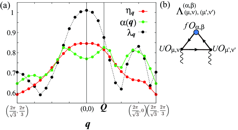
Figure S11: (a) ${{\bm{q}}}$ dependences of spin-channel eigenvalue $\eta_{{\bm{q}}}$ and the charge-channel one $\lambda_{{\bm{q}}}$ obtained by the DW equations. The RPA Stoner factor at ${{\bm{q}}}$, ${\alpha}({{\bm{q}}})$, is also shown. Model parameters are $n=2.0$ and $\alpha=0.83$. (b) Three-point vertex in AL term, where $O_{{\alpha},{\beta}}$, $O_{\mu,\nu}$, and $O_{\mu^{\prime},\nu^{\prime}}$ are the spin-valley operators.

I.8 H: Effects of off-site Coulomb interaction on the nematic order

In the main text, we studied the MATBG Hubbard model with on-site Coulomb interaction $U$. However, off-site Coulomb interactions are not small because of the large size of the Wannier function in MATBG; its size exceeds the AB-BA distance in Fig. 1 (b) [1, 10]. The Coulomb interaction term is given as

$$H^{\prime}=U\sum_{i}n_{i\uparrow}n_{i\downarrow}+\frac{1}{2}\sum_{i\neq j}V_{i,j}n_{i}n_{j},$$ (S21)

where $n_{i{\sigma}}$ is the ${\sigma}$-spin electron number operator at site $i$, $n_{i}=n_{i\uparrow}+n_{i\downarrow}$, and $V_{i,j}$ is the off-site Coulomb interaction. (We drop the inter-site density terms.) Authors in Ref. [10] derived the Coulomb interaction by considering the screening due to the metallic gate. Then, approximately, the ratio between the nearest, the next nearest, and the third nearest Coulomb potential is $V_{1}:V_{2}:V_{3}=2:1:1$, and the ratio $r\equiv V_{1}/U$ is $2/3$.

In the main text, we studied the case of $r=0$. Now, we discuss the effect of the off-site Coulomb interaction ($r\neq 0$) on the nematicity. Here, we study the case of $r\ll 2/3$ because the effective $r$ will be reduced by the Thomas-Fermi screening due to the conduction electrons of MATBG.

Hereafter, we consider $r$ as a parameter and fix the ratio $V_{1}:V_{2}:V_{3}=2:1:1$ for simplicity. The bare interaction by $V_{n}$ is expressed as

$$I^{V,{{\bm{q}}}}_{ll^{\prime},mm^{\prime}}(k,k^{\prime}) = -2V_{l,m}({{\bm{q}}})\delta_{l,l^{\prime}}\delta_{m,m^{\prime}}$$

$$+V_{l,l^{\prime}}({{\bm{k}}}-{{\bm{k}}}^{\prime})\delta_{l,m}\delta_{l^{\prime},m^{\prime}},$$

where $V_{l,m}({{\bm{k}}})$ is the Fourier transformation of $V_{i,j}$, and $l,m=1\sim 4$. The first and the second terms in Eq. (LABEL:eqn:IV) correspond to the Hartree and the Fock terms, respectively.

Here, we introduce ${\hat{I}}^{V,{{\bm{q}}}}$ in Eq. (LABEL:eqn:IV) into the irreducible interaction ${\hat{I}}^{c,{{\bm{q}}}}$ in Eq. (S6) to discuss the effect of $V_{n}$ on the nematicity. (Unfortunately, serious diagrammatic calculation of the MT and AL terms in the $U+\{V_{n}\}$ Hubbard model is very difficult.) Figure S12 exhibits the eigenvalue of charge-channel DW equaiton with the irreducible interaction ${\hat{I}}^{c,{{\bm{q}}}}(k,k^{\prime})+{\hat{I}}^{V,{{\bm{q}}}}(k,k^{\prime})$. We see that the nematic order eigenvalue at ${{\bm{q}}}={\bm{0}}$ linearly increases with $r\equiv V_{1}/U$. Thus, the nematic order due to the AL process is stabilized by finite $V_{n}$, due to the Fock term in Eq. (LABEL:eqn:IV). (In contrast, the Stoner factor ${\alpha}$ is independent of $V$ for $r<0.3$.)

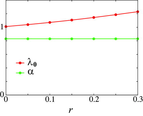
Figure S12: Obtained charge-channel eigenvalue $\lambda_{{{\bm{q}}}={\bm{0}}}$ and Stoner factor ${\alpha}$ as functions of $r=V_{1}/U$. $\lambda_{\bm{0}}$ linearly increases with $r$, while ${\alpha}$ is independent of $r$.

Thus, we conclude that the driving force of the ferro-nematic order in MATBG is the valley + spin fluctuation interference mechanism, and finite off-site Coulomb potential will stabilize the nematic order. We stress that the Hartree-Fock term alone in Eq. (LABEL:eqn:IV) yields the density-wave order with ${{\bm{q}}}\neq\bm{0}$. Note that ${\alpha}_{c}=1$ is satisfied when $r=0.75$ in the RPA Therefore, the present $SU(4)$ interference mechanism is essential for the ${{\bm{q}}}=\bm{0}$ nematic order.

References

[1]
Y. Cao, V. Fatemi, S. Fang, K. Watanabe, T. Taniguchi, E. Kaxiras, and
P. Jarillo-Herrero, Nature 556, 43 (2018).
[2]
Y. Cao, V. Fatemi, A. Demir, S. Fang, S. L. Tomarken, J. Y. Luo,
J. D. Sanchez-Yamagishi, K. Watanabe, T. Taniguchi, E. Kaxiras,
R. C. Ashoori, and
P. Jarillo-Herrero, Nature 556, 80 (2018).
[3]
M. Yankowitz, S. Chen, H. Polshyn, Y. Zhang, K. Watanabe, T. Taniguchi,
D. Graf, A. F. Young, and C. R. Dean, Science 363, 1059
(2019).
[4]
X. Lu, P. Stepanov, W. Yang, M. Xie, M. A. Aamir, I. Das,
C. Urgell, K. Watanabe, T. Taniguchi, G. Zhang, A. Bachtold,
A. H. MacDonald, and D. K. Efetov, Nature 574, 653 (2019).
[5]
C. Xu and L. Balents, Phys. Rev. Lett. 121, 087001 (2018).
[6]
J. F. Dodaro, S. A. Kivelson, Y. Schattner, X. Q. Sun, and C. Wang,
Phys. Rev. B 98, 075154 (2018).
[7]
J. W. F. Venderbos and R. M. Fernandes, Phys. Rev. B 98, 245103 (2018).
[8]
H. Isobe, N. F. Q. Yuan, and L. Fu, Phys. Rev. X 8, 041041 (2018).
[9]
J. Kang and O. Vafek, Phys. Rev. Lett. 122, 246401 (2019).
[10]
K. Seo, V. N. Kotov, and B. Uchoa, Phys. Rev. Lett. 122, 246402
(2019).
[11]
Y.-P. Lin and R. M. Nandkishore,
Phys. Rev. B 100, 085136 (2019).
[12]
B. Roy and V. Juricic, Phys. Rev. B 99, 121407(R) (2019).
[13]
S. Ray, J. Jung, and T. Das, Phys. Rev. B 99, 134515 (2019).
[14]
Y.-Z. You and A. Vishvanath, npj Quantum Mater. 4, 16 (2019).
[15]
Y.-H. Zhang, D. Mao, and T. Senthil, Phys. Rev. Research 1, 033126 (2019).
[16]
D. V. Chichinadze, L. Classen, and A. V. Chubukov, Phys. Rev. B 101, 224513 (2020).
[17]
Y. Wang, J. Kang, and R. M. Fernandes, Phys. Rev. B 103, 024506 (2021).
[18]
M. Xie and A. H. MacDonald, Phys. Rev. Lett. 124, 097601 (2020).
[19]
N. Bultinck, S. Chatterjee and M. P. Zaletel, Phys. Rev. Lett. 124, 166601 (2020).
[20]
A. Kerelsky, L. McGilly, D. M. Kennes, L. Xian, M.
Yankowitz, S. Chen, K. Watanabe, T. Taniguchi, J. Hone,
C. Dean, A. Rubio, and A. N. Pasupathy,
Nature 572, 95 (2019).
[21]
Y. Choi, J. Kemmer, Y. Peng, A. Thomson, H. Arora,
R. Polski, Y. Zhang, H. Ren, J. Alicea, G. Refael, F. von Oppen,
K. Watanabe, T. Taniguchi, and S. Nadj-Perge,
Nat. Phys. 15, 1174 (2019).
[22]
Y. Jiang, X. Lai, K. Watanabe, T. Taniguchi,
K. Haule, J. Mao, and E. Y. Andrei,
Nature 573, 91 (2019).
[23]
Y. Cao, D. R. Legrain, J. M. Park, F. N. Yuan, K.
Watanabe, T. Taniguchi, R. M. Fernandes, L. Fu,
P. J. Herrero, Science 372, 264 (2021).
[24]
R. M. Fernandes and J. W. F. Venderbos, Sci. Adv. 6 eaba8834 (2020).
[25]
J. W. F. Venderbos and R. M. Fernandes,
Phys. Rev. B 98, 245103 (2018).
[26]
D. V. Chichinadze, L. Classen, and A. V. Chubukov, Phys. Rev. B 102, 125120 (2020).
[27]
D. C. Johnston, Adv. Phys. 59, 803 (2010)
[28] Y. Mizuguchi and Y. Takano,
J. Phys. Soc. Jpn. 79, 102001 (2010).
[29]
Y. Sato S. Kasahara, H. Murayama, Y. Kasahara, E.-G. Moon,
T. Nishizaki, T. Loew, J. Porras, B. Keimer, T. Shibauchi, and
Y. Matsuda, Nat. Phys. 13, 1074 (2017).
[30]
E. Fradkin, S. A. Kivelson, and J. M. Tranquada, Rev. Mod. Phys. 87, 457 (2015).
[31]
J. C. S. Davis and D.-H. Lee, Proc. Natl. Acad. Sci. USA 110,
17623 (2013).
[32]
R. M. Fernandes, L. H. VanBebber, S. Bhattacharya, P. Chandra,
V. Keppens, D. Mandrus, M. A. McGuire, B. C. Sales, A. S. Sefat,
and J. Schmalian,
Phys. Rev. Lett. 105, 157003 (2010).
[33]
R. M. Fernandes, E. Abrahams, and J. Schmalian,
Phys. Rev. Lett. 107, 217002 (2011).
[34]
F. Wang, S. A. Kivelson, and D.-H. Lee,
Nat. Phys. 11, 959 (2015).
[35]
R. Yu, and Q. Si,
Phys. Rev. Lett. 115, 116401 (2015).
[36]
J. K. Glasbrenner, I. I. Mazin, H. O. Jeschke, P. J. Hirschfeld, and R. Valenti,
Nat. Phys. 11, 953 (2015).
[37]
C. Fang, H. Yao,W.-F. Tsai, J. P. Hu, and S. A. Kivelson,
Phys. Rev. B 77, 224509 (2008).
[38]
R. M. Fernandes and A. V. Chubukov, Rep. Prog. Phys. 80, 014503 (2017).
[39]
F. Krüger, S. Kumar, J. Zaanen, J. van den Brink, Phys. Rev. B 79, 054504 (2009).
[40]
W. Lv, J. Wu, and P. Phillips,
Phys. Rev. B 80, 224506 (2009).
[41]
C.-C. Lee, W.-G. Yin, and W. Ku,
Phys. Rev. Lett. 103, 267001 (2009).
[42]
H. Kontani and S. Onari,
Phys. Rev. Lett. 104, 157001 (2010).
[43]
S. Onari and H. Kontani,
Phys. Rev. Lett. 109, 137001 (2012).
[44]
S. Onari, Y. Yamakawa, and H. Kontani,
Phys. Rev. Lett. 116, 227001 (2016).
[45]
Y. Yamakawa, S. Onari and H. Kontani, Phys. Rev. X 6, 021032
(2016).
[46]
S. Onari and H. Kontani, Phys. Rev. B 100, 020507(R) (2019).
[47]
K. Jiang, J. Hu, H. Ding, and Z. Wang,
Phys. Rev. B 93, 115138 (2016).
[48]
L. Fanfarillo, G. Giovannetti, M. Capone, and E. Bascones,
Phys. Rev. B 95, 144511 (2017).
[49]
R. Q. Xing, L. Classen, A. V. Chubukov, Phys. Rev. B 98, 041108(R) (2018).
[50]
A. V. Chubukov, M. Khodas, and R. M. Fernandes,
Phys. Rev. X 6, 041045 (2016).
[51]
M. Tsuchiizu, K. Kawaguchi, Y. Yamakawa, and H. Kontani, Phys. Rev. B
97, 165131 (2018).
[52]
M. Tsuchiizu, Y. Ohno, S. Onari, and H. Kontani,
Phys. Rev. Lett. 111, 057003 (2013).
[53]
M. Koshino, N. F. Q. Yuan, T. Koretsune, M. Ochi, K. Kuroki, and L. Fu,
Phys. Rev. X 8, 031087 (2018).
[54]
M. J. Klug, New J. Phys. 22, 073016 (2020).
[55]
Supplemental Material
[56]
H. Kontani, Y. Yamakawa, R. Tazai, and S. Onari, Phys. Rev. Research
3, 013127 (2021).
[57]
J. M. Luttinger and J. C. Ward, Phys. Rev. 118, 1417
(1960).
[58]
G. Baym and L. P. Kadanoff, Phys. Rev. 124, 287
(1961).
[59]
R. Tazai, Y. Yamakawa, and H. Kontani, Phys. Rev. B 103, L161112
(2021).
[60]
R. Tazai and H. Kontani, Phys. Rev. B 100, 241103(R) (2019).
[61]
H. Kontani, T. Saito, and S. Onari,
Phys. Rev. B 84, 024528 (2011).

References

[1]
M. Koshino, N. F. Q. Yuan, T. Koretsune, M. Ochi, K. Kuroki, and L. Fu,
Phys. Rev. X 8, 031087 (2018).
[2]
A. Kerelsky, L. McGilly, D. M. Kennes, L. Xian, M.
Yankowitz, S. Chen, K. Watanabe, T. Taniguchi, J. Hone,
C. Dean, A. Rubio, and A. N. Pasupathy,
Nature 572, 95 (2019).
[3]
M. J. Klug, New J. Phys. 22, 073016 (2020).
[4]
S. Onari, Y. Yamakawa, and H. Kontani,
Phys. Rev. Lett. 116, 227001 (2016).
[5]
S. Onari and H. Kontani, Phys. Rev. B 100, 020507(R) (2019).
[6]
J. M. Luttinger and J. C. Ward, Phys. Rev. 118, 1417
(1960).
[7]
G. Baym and L. P. Kadanoff, Phys. Rev. 124, 287 (1961).
[8]
R. Tazai and H. Kontani, Phys. Rev. B 100, 241103(R) (2019).
[9]
H. Kontani, Y. Yamakawa, R. Tazai, and S. Onari, Phys. Rev. Research
3, 013127 (2021).
[10]
J. Kang and O. Vafek, Phys. Rev. Lett. 122, 246401 (2019).
[11]
Y. Wang, J. Kang, and R. M. Fernandes, Phys. Rev. B 103, 024506 (2021).