Risk-Aware Submodular Optimization for
Stochastic Travelling Salesperson Problem

Abstract

We introduce a risk-aware variant of the Traveling Salesperson Problem (TSP), where the robot tour cost and reward have to be optimized simultaneously, while being subjected to uncertainty in both. We study the case where the rewards and the costs exhibit diminishing marginal gains, i.e., are submodular. Since the costs and the rewards are stochastic, we seek to maximize a risk metric known as Conditional-Value-at-Risk (CVaR) of the submodular function. We propose a Risk-Aware Greedy Algorithm (RAGA) to find an approximate solution for this problem. The approximation algorithm runs in polynomial time and is within a constant factor of the optimal and an additive term that depends on the value of optimal solution. We use the submodular function’s curvature to improve approximation results further and verify the algorithm’s performance through simulations.

I Introduction

Determining an optimal tour to visit all the locations in a given set while minimizing/maximizing a metric is the classical Travelling Salesperson Problem (TSP) that finds applications in robotics, logistics, etc. However, there are several applications where the environment is dynamic and uncertain, as a result of which classical approaches to solving the TSP are insufficient. Examples include determining routes to visit active volcanic regions (where the activity has temporal variability) for obtaining scientific information (as shown in Fig. 1); determining routes for a logistic delivery vehicle in dense urban regions with uncertain traffic, etc. In such scenarios, the risk due to uncertainty in the travel times and/or the rewards collected along the path needs to be considered while determining the tour.

Several approaches to stochastic TSP have been presented in the literature. In [perboli2017progressive], a two-step process to convert the TSP to a multi-integer linear programming problem and then introduce a meta-heuristic based on the probabilistic hedging method proposed in [rockafellar1991scenarios] is carried out. Paulin [paulin2014convex] uses an extension of Stein’s method for exchangeable pairs to approach the stochastic salesperson problem. In [maity2015modified], [maity2016imprecise] and [mukherjee2019constrained], the authors develop a genetic algorithm to approach the uncertainty in TSP. In [itani2007stochastic], a constant factor approximation algorithm is developed for a Dubin’s vehicle visiting all the points, with cost minimization being the main objective. In [adler2016stochastic], again an approximation algorithm is presented to minimize the time taken to visit the targets that are appearing stochastically in the environment. In all the above articles, the risk is not considered directly.

We argue that a different approach is necessary in many risk-sensitive applications. Specifically, instead of optimizing the expected cost, optimizing a risk-sensitive measure may be more appropriate. In this paper, we focus on this case and present a risk-aware TSP formulation. To do so, we develop an approximation to the stochastic TSP with the optimization objective represented as a submodular function. The resulting algorithm takes as input a risk tolerance parameter, $\alpha$, and produces a tour that maximizes the expected behavior in the worst $\alpha$ percentile cases. Thus, the user can choose tours ranging from risk-neutral ($\alpha=1$) to very conservative ($\alpha\approx 0$).

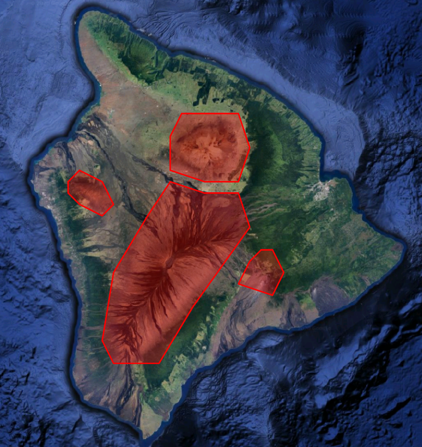
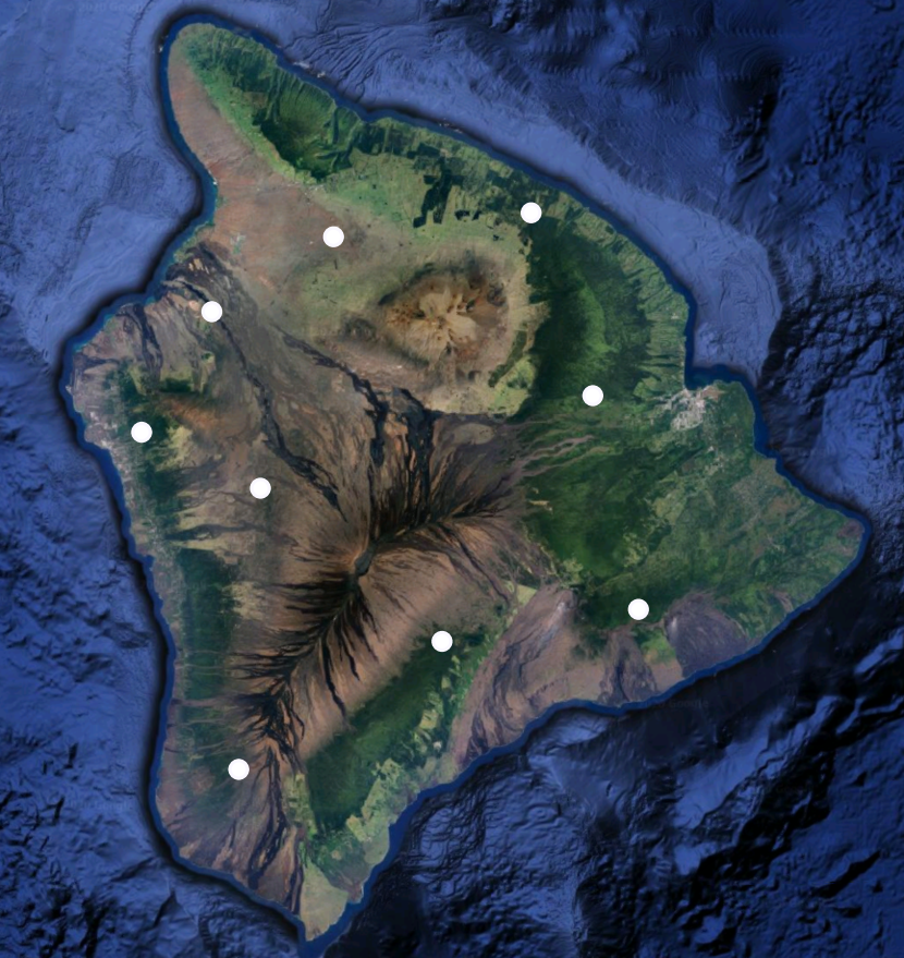
(a) An image of an island, with the locations of active volcanoes highlighted in red

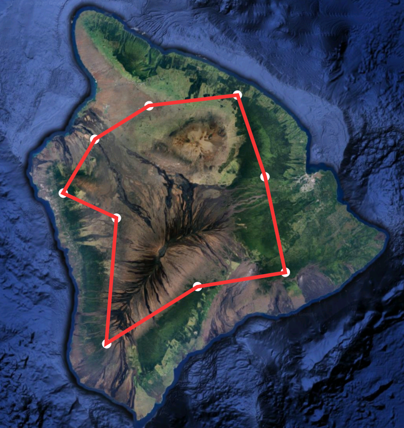
(b) Key sites of surveillance surrounding the volcanic sites

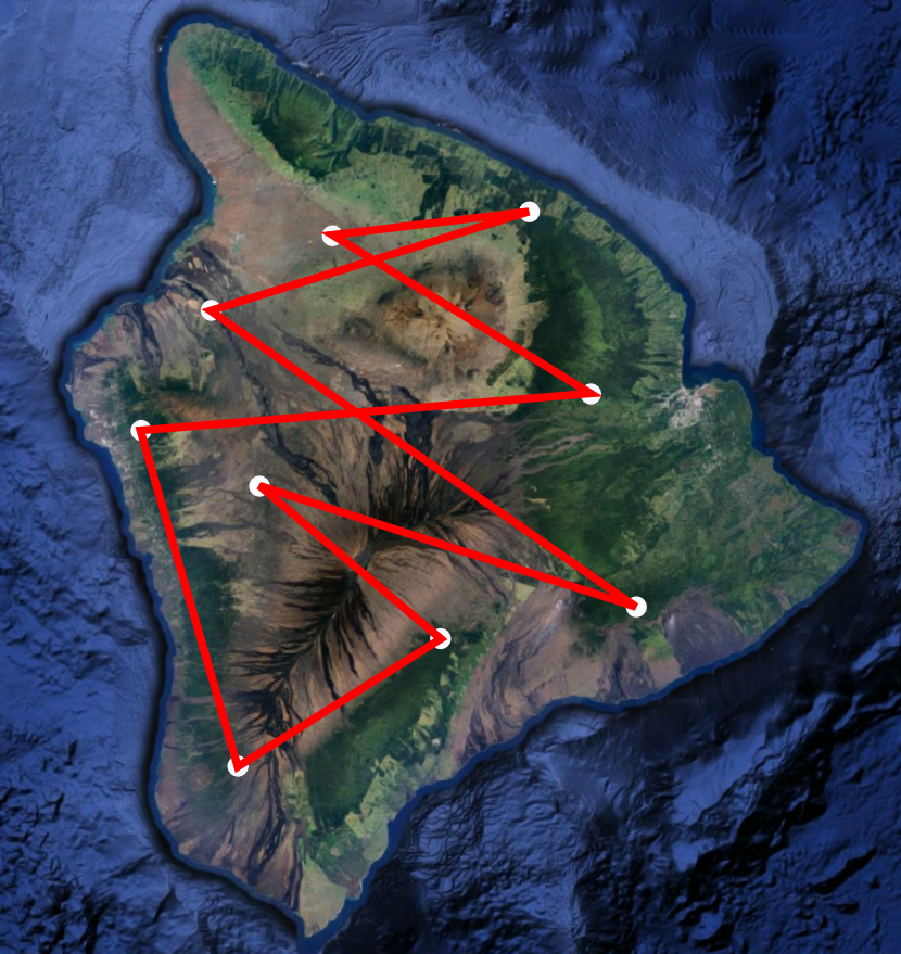
(c) Tour with low cost and low reward

(d) Tour with high cost and high reward

Figure 1: An example of risk-aware tour selection for volcano monitoring in an island. A low-risk, low-reward monitoring tour avoids the more interesting region in the middle which the high-risk, high-reward tour covers.

An important property of submodular functions are their diminishing marginal values. The use of submodular functions is wide-spread: from information gathering [krause2011submodularity] and image segmentation [boykov2001interactive] to document summarization [lin2011class]. Rockafellar and Uryasev [rockafellar2000optimization] introduce a relationship between a submodular function and the Conditional-Value-at-Risk (CVaR). CVaR is a risk metric that is commonly employed in stochastic optimization in finance and stock portfolio optimization. Another popular measure of risk is the Value-at-Risk (VaR) [morgan1997creditmetrics], which is commonly used to formulate the chance-constrained optimization problems. In [yang2017algorithm], and [yang2018algorithm], the authors study the chance-constrained optimization problem while also considering risk in the multi-robot assignment, and then extend it to a knapsack formulation. In a comparison between the VaR and CVaR, Majumdar and Pavone [majumdar2020should] propose that the CVaR is a better measure of risk for robotics, especially when the risk can cause a huge loss. In [zhou2018approximation] and [zhou2020risk], a greedy algorithm for maximizing the CVaR is proposed.

Building on the work by [zhou2018approximation, zhou2020risk], in this paper, we develop a polynomial-time algorithm for approximating a solution to the stochastic TSP. Our method differs from the previous approaches due to the presence of uncertainty in the tour cost, making traditional path-planning algorithms fail. The framework presented in [zhou2018approximation, zhou2020risk] is effective only for one-stage planning (selecting a path amongst a set of candidate paths). In this paper, we present a multi-stage planner that finds a route taking the stochastic aspect into account. To achieve this, we propose an objective function that balances risk and reward for a tour and prove that this function is submodular. The method in [jawaid2013maximum] addresses the deterministic TSP with a reward-cost trade-off, while our work is focused on a stochastic version where the uncertainty in reward and cost is considered. The algorithm from [jawaid2013maximum] can be viewed as a special case of our algorithm, with $\alpha=1$ and the subsequent risk ignored.

Contributions: The main contributions of this paper are:

• We present a risk-aware TSP with a stochastic objective that balances risk and reward for planing a TSP tour (Problem 1).

• We show the objective is submodular (Lemma 3) and propose a greedy algorithm (RAGA) to find tours that maximize the CVaR of a stochastic objective (Algorithm 1).

• We prove that the solution obtained by RAGA is within a constant approximation factor of the optimal and an additive term proportional to the optimal solution (Theorem 1) and prove that RAGA has a polynomial run-time (Theorem LABEL:thm:complexity).

• We evaluate the performance of the algorithm through extensive simulations (Section LABEL:sec:_results).

II Preliminaries

We first introduce the conventions and notations used in this paper. Calligraphic capital letters denote sets (e.g. $\mathcal{A}$). $2^{\mathcal{A}}$ denotes the power set of $\mathcal{A}$ and $|\mathcal{A}|$ represents its cardinality. Given a set $\mathcal{B}$, $\mathcal{A\setminus B}$ denotes set difference. Let $x$ be a random variable, then $\mathbb{E}[x]$ represents the expectation of the random variable $x$, and $\mathbb{P[\cdot]}$ denotes its probability.

II-A Set and Function Properties

Optimization problems generally work over a set system $(\mathcal{X,Y})$ where $\mathcal{X}$ is the base set and $\mathcal{Y}\subseteq 2^{\mathcal{X}}$. A reward/cost function $f:\mathcal{Y}\rightarrow\mathbb{R}$ is then either maximized or minimized.

Definition 1

(Monotonically Increasing): A set function $f:\mathcal{Y}\rightarrow\mathbb{R}$ is said to be monotonically increasing if and only if for any set $\mathcal{S^{\prime}}\subseteq\mathcal{S}\in 2^{\mathcal{X}},\leavevmode\nobreak\ f(\mathcal{S^{\prime}})<f(\mathcal{S})$.

Definition 2

(Submodularity): A function $f:2^{\mathcal{X}}\rightarrow\mathbb{R}$ is submodular if and only if
$f(\mathcal{S})+f(\mathcal{T})\geq f(\mathcal{S}\cup\mathcal{T})+f(\mathcal{S}\cap\mathcal{T}),\leavevmode\nobreak\ \forall\mathcal{S},\mathcal{T}\in 2^{\mathcal{X}}$.

Definition 3

(Matroid): An independence set system $\mathcal{(X,Y)}$ is called a matroid if for any sets $\mathcal{S,P}\in 2^{\mathcal{X}}$ and $|\mathcal{P}|\leq|\mathcal{S}|$, it must hold that there exists an element $s\in\mathcal{S}\setminus\mathcal{P}$ such that $\mathcal{P}\cup\{s\}\in\mathcal{Y}$.

Definition 4

(Curvature): Curvature is used as a measure of the degree of submodularity of a function $f$. Consider the matroid pair $(\mathcal{X,Y})$, and a function $f:2^{\mathcal{X}}\rightarrow\mathbb{R}$, such that for any element $s\in\mathcal{X},f(\{s\})\neq 0$. The curvature $k,0\leq k\leq 1$ is then defined as:

$$k=1-\min_{s\in\mathcal{S},\mathcal{S}\in\mathcal{Y}}\>\frac{f(\mathcal{S})-f(\mathcal{S}\setminus\{s\})}{f(\{s\})}.$$ (1)

II-B Travelling Salesperson Problem

Definition 5

(TSP): Given a complete graph $G(\mathcal{V,E})$, the objective of the TSP is to find a minimum cost (maximum reward) Hamiltonian cycle.

In this paper, we consider the symmetric undirected TSP, where each edge has a reward and cost associated with it.

II-C Measure of Risk

Let $f(\mathcal{S},y)$ denote a utility function with solution set $\mathcal{S}$ and noise $y$. As a result of $y$, the value of $f(\mathcal{S},y)$ is a random variable for every $\mathcal{S}$.

Definition 6

(Value at Risk): The Value at Risk (VaR) is defined as:

$$\emph{VaR}_{\alpha}(\mathcal{S})=\min_{\tau\in\mathbb{R}}\;\{\mathbb{P}[f(\mathcal{S},y)\leq\tau]\geq\alpha\},\;\alpha\in(0,1],$$ (2)

where $\alpha$ is the user-defined risk-level. A higher value of $\alpha$ corresponds to the choice of a higher risk level.

Definition 7

(Conditional Value at Risk): The Conditional-Value-at-Risk (CVaR) is defined as

$$\emph{CVaR}_{\alpha}(\mathcal{S})=\mathbb{E}_{y}[f(\mathcal{S},y)\>|\>f(\mathcal{S},y)\leq\emph{VaR}_{\alpha}(\mathcal{S})].$$ (3)

Maximizing the value of $\text{CVaR}_{\alpha}(\mathcal{S})$ is equivalent to maximizing the auxiliary function $H(\mathcal{S},\tau)$ (Theorem 2, [rockafellar2000optimization]):

$$H(\mathcal{S},\tau)=\tau-\frac{1}{\alpha}\mathbb{E}_{y}[\>(\tau-f(\mathcal{S},y))^{+}\>],$$ (4)

where $[t]^{+}=t,\leavevmode\nobreak\ \forall t\geq 0$ and $0$ when $t<0$.

Lemma 1

(Lemma 1, [zhou2018approximation]) If $f(\mathcal{S},y)$ is monotone increasing, submodular and normalized in set $\mathcal{S}$ for any realization of $y$, then the auxiliary function $H(\mathcal{S},\tau)$ is monotone increasing and submodular but not necessarily normalized in set $\mathcal{S}$ for any given $\tau$.

Lemma 2

(Lemma 2, [zhou2018approximation]) The auxiliary function $H(\mathcal{S},\tau)$ is concave in $\tau,\forall\>\mathcal{S}$.

III Problem Formulation

In this section, we first discuss a risk-aware TSP and then formulate the problem as a stochastic optimization problem by using CVaR.

III-A Risk-Aware TSP

In order to motivate our formulation, consider the scenario of monitoring active volcanoes using a robot (say aerial robot) on an island as shown in Fig. 1, where the red-colored patches represent active volcanic regions. The important sites ($\mathcal{V}$) that the robot needs to visit are shown in Fig. 1. These sites are strategic positions from which it is possible to observe the volcanic situation from a safe distance. The robot travels between these monitoring sites and receives a reward based on the information gathered while traversing this tour. In this work, we do not constrain vehicle motion in terms of distance or time. While traveling directly above the volcano, the robot faces a higher chance of failure (due to volcanic activity) but can gather more information (a higher reward), while traveling along a shorter path (less cost). On the other hand, while traveling around the volcano, the robot has a lower risk but must travel a longer distance (more cost) while also receiving a lower reward. Fig. 1 and Fig. 1 show the paths that could be adopted based on the risk level specified for the robot. Our objective is to find a suitable tour for a single robot while considering the risk threshold and the trade-off between path cost and reward required.

The monitoring task is modeled as a risk-aware TSP on a graph $G(\mathcal{V},\mathcal{E})$ of an environment ${E}$ with $|\mathcal{V}|$ sites of interest. The notation $\mathcal{E}$ represents the set of edges connecting the vertices. A representative information density map ${M}$ of the environment ${E}$ is shown in Fig. 2. The robot has sensors with a sensing range $R$. As it travels along the tour, the robot receives a reward based on the amount of information it collects and a penalty proportional to the tour’s cost. We assume that both the reward and cost are random variables, with the reward being positive, and the cost of every edge having an upper-bound of $C$. We use $r(\mathcal{S},y_{r})$ and $c(\mathcal{S},y_{c})$ to denote the reward and cost for a set of edges $\mathcal{S}$, where $r(\mathcal{S})$ and $c(\mathcal{S})$ are the sum of rewards of all points observed and the costs incurred when travelling along the edges in set $\mathcal{S}$ respectively, and $y_{r}$ and $y_{c}$ are the respective noises induced.

As we want to minimize cost and maximize reward simultaneously, our utility function $f(\mathcal{S},y)$ is a combination of these two terms, with a weighting factor deciding the priority we place on the cost over the reward. We define $f(\mathcal{S},y)$ as

$$f(\mathcal{S},y)=(1-\beta)\>r(\mathcal{S},y_{r})+\beta\>(|\mathcal{S}|C-c(\mathcal{S},y_{c})),$$ (5)

where $\beta\in[0,1]$ is the weighting parameter. When $\beta=0$, we ignore the cost incurred and consider the rewards received only. When $\beta=1$, we ignore the rewards and are wary of only the cost penalized (classical TSP). Note that we directly incorporate the cost-reward trade-off into the utility function.

Let us define $r(\mathcal{S},y_{r})$ as $f_{r}(\mathcal{S},y_{r})$ and $|\mathcal{S}|C-c(\mathcal{S},y_{c})$ as $f_{c}(\mathcal{S},y_{c})$.

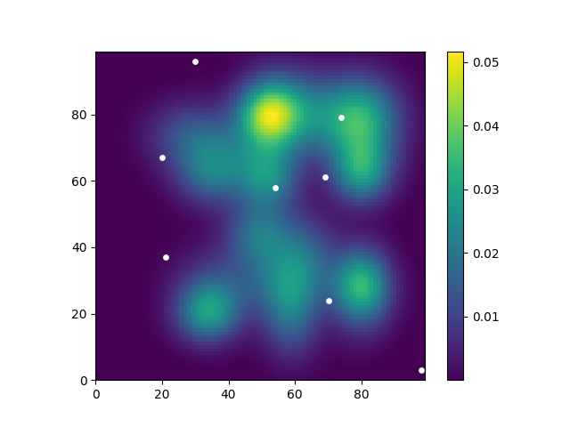
Figure 2: Map $M$ shows the information distribution in the environment $E$. The right bar shows the density degree of the information.

Lemma 3

The utility function $f(\mathcal{S},y)$ is both submodular and monotone increasing in $\mathcal{S}$.

Proof:

Let $e$ be the edge to be added to the tour, where $e\in\mathcal{E}\setminus\mathcal{S}$ and $\mathcal{S}$ is set of edges selected so far. Let us consider the two parts of $f(\mathcal{S},y)$ separately.

$f_{r}(\mathcal{S},y)$

• As the rewards are sampled from a truncated Gaussian, with a lower bound of 0, they are thus always positive. Therefore, $f_{r}(\mathcal{S},y)$ is always monotone increasing in $\mathcal{S}$,

  $$f_{r}(\mathcal{S})\leq f_{r}(\mathcal{S}\cup\{e\}).$$ (6)

• While calculating the total reward, we add the rewards obtained from all distinct points observed while traversing this tour. Consider the current set of edges $\mathcal{S}$ and a new edge $e$. If the new edge $e$ and the edges $\mathcal{S}$ have any overlap in the sensed regions, the total reward received from traversing $\mathcal{S}$ and $e$ successively will be less than the sum of rewards of traversing $\mathcal{S}$ and $e$ individually. Therefore,

  $$f_{r}(\mathcal{S}\cup\{e\})\leq f_{r}(\mathcal{S})+f_{r}(\{e\}).$$

  Also, since $e\in\mathcal{E}\setminus\mathcal{S}$, $f_{r}(\mathcal{S}\cap\{e\})=0$. Then we have,

  $$f_{r}(\mathcal{S}\cup\{e\})+f_{r}(\mathcal{S}\cap\{e\})\leq f_{r}(\mathcal{S})+f_{r}(\{e\}),$$ (7)

  and thus $f_{r}(\mathcal{S},y)$ is submodular in $\mathcal{S}$.

$f_{c}(\mathcal{S},y)$

• The cost of each edge is defined as a truncated Gaussian with a upper bound of $M_{c}$. For any set of edges in $\mathcal{S}$, the sum of costs will always be less than $|\mathcal{S}|M_{c}$, which means any sample (realization) of $f_{c}(\mathcal{S},y)$ is positive. Therefore, $f_{c}(\mathcal{S},y)$ is always monotone increasing in $\mathcal{S}$, i.e.,

  $$f_{c}(\mathcal{S})\leq f_{c}(\mathcal{S}\cup\{e\}).$$ (8)

• Consider again, the current set of edges $\mathcal{S}$ and the new edge $e$. The total cost of traversing $\mathcal{S}$ and $e$ is equal to the sum of costs of traversing $\mathcal{S}$ and $e$ individually. Therefore,

  $$f_{c}(\mathcal{S}\cup\{e\})=f_{c}(\mathcal{S})+f_{c}(\{e\}),$$ (9)

  and thus $f_{c}(\mathcal{S},y)$ is modular in $\mathcal{S}$.

$f(\mathcal{S},y)$

Since both $f_{r}(\mathcal{S},y_{r})$ and $f_{c}(\mathcal{S},y_{c})$ are monotone increasing in $\mathcal{S}$, $f(\mathcal{S},y)$ as the summation of these two, is also monotone increasing in $\mathcal{S}$. Similarly, since $f_{r}(\mathcal{S},y_{r})$ is submodular in $\mathcal{S}$ and $f_{c}(\mathcal{S},y_{c})$ is modular in $\mathcal{S}$, $f(\mathcal{S},y)$ as the summation of these two, is submodular in $\mathcal{S}$. $\Box$

III-B Risk-Aware Submodular Maximization

Consider the set system $\mathcal{(E,I)}$, where $\mathcal{E}$ is the set of all edges in the graph $G(\mathcal{V,E})$. If $\mathcal{A}_{1},\mathcal{A}_{2}\ldots\mathcal{A}_{n}$ each contains the edges forming $n$ Hamiltonian tours, then $\mathcal{I}:=2^{\mathcal{A}_{1}}\cup 2^{\mathcal{A}_{2}}\ldots\cup 2^{\mathcal{A}_{n}}$. We define our risk-aware TSP by maximizing $\text{CVaR}_{\alpha}(\mathcal{S})$, where $\mathcal{S}\in\mathcal{I}$. We know that maximizing the $\text{CVaR}_{\alpha}(\mathcal{S})$ is equivalent to maximizing the auxiliary function ${H(\mathcal{S},\tau)}$. Thus, we formally define the problem as:

Problem 1 (Risk-aware TSP)

$$\max_{\mathcal{S}\in\mathcal{I},\leavevmode\nobreak\ \tau\in[0,\Gamma]}\tau-\frac{1}{\alpha}\mathbb{E}_{y}[(\tau-f(\mathcal{S},y))^{+}],$$ (10)

where $\Gamma$ is the upper bound on the value of $\tau$.

IV Algorithm And Analysis

Input:

  Graph $G(\mathcal{V,E})$; Risk level $\alpha\in(0,1]$; Weighing factor $\beta\in[0,1]$; Upper bound $\Gamma\in\mathbb{R}^{+}$ on $\tau$; Searching factor $\gamma\in(0,\Gamma]$; Oracle function $\mathbb{O}$ that approximates $H(\mathcal{S},\tau)$ as $\hat{H}(\mathcal{S},\tau)$.

Output:

  A Hamiltonian tour $S^{G}$ and its respective $\tau^{G}$.

1 for i = {0, 1, 2, . . ., $\left\lceil\frac{\Gamma}{\gamma}\right\rceil$} do

2       $\mathcal{S}=\emptyset$; $D=\mathbf{0}_{1\times|\mathcal{V}|}$; $\hat{H}_{\text{max}}=0$; $\hat{H}_{\text{cur}}=0$

3       $\tau_{i}=i\,\gamma$

4       while  $\mathcal{E}\neq\emptyset$ and $\mathcal{|S|}\leq|\mathcal{V}|$ do

5             $e^{\star}=\text{argmax}_{{\forall e\in\mathcal{E}\setminus\mathcal{S}}}\;\hat{H}(\mathcal{S}\cup\{e\},\tau_{i})-\hat{H}(\mathcal{S},\tau_{i})$

6             $(u,v)\leftarrow\mathcal{V}(e^{\star})$

7             $\text{flag}=\texttt{False}$

8             if $D[u]<2$ and $D[v]<2$ then

9                   check subtour existence in $\mathcal{S}\cup\{e^{\star}\}$ by running DFS

10                   if no subtour present then

11                         $\text{flag}=\texttt{True}$

12                   end if

13                  

14             end if

15             if $\text{flag}==\texttt{True}$ then

16                   $\mathcal{S}\leftarrow\mathcal{S}\cup\{e^{\star}\}$

17                   $D[u]+=1$; $D[v]+=1$

18                   $\hat{H}_{\text{cur}}=\hat{H}(\mathcal{S}\cup\{e^{\star}\},\tau_{i})$

19             end if

20             $\mathcal{E}\leftarrow\mathcal{E}\setminus\{e^{\star}\}$

21       end while

22       if $\hat{H}_{\text{cur}}\geq\hat{H}_{\text{max}}$ then

23             $\hat{H}_{\text{max}}=\hat{H}_{\text{cur}}$; $(\mathcal{S}^{G},\tau^{G})=(\mathcal{S},\tau_{i})$

24       end if

25       if $\hat{H}_{\text{cur}}<0$ then

26             break

27       end if

28      

29 end for

Algorithm 1 Risk-aware greedy algorithm (RAGA)

In this section, we present a risk-aware greedy algorithm (RAGA) that extends the deterministic algorithm in [jawaid2013maximum] for solving Problem 1. We first explicitly introduce RAGA, then analyze its performance in terms of approximation bound and running efficiency.

(a) $\beta=0$

(b) $\beta=0.4$

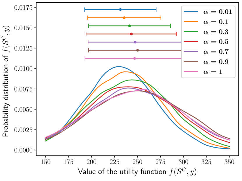
(c) $\beta=0.7$

(d) $\beta=1$

Figure 3: Probability density function of $f(\mathcal{S},y)$ at different values of $\alpha$, keeping $\beta$ fixed.

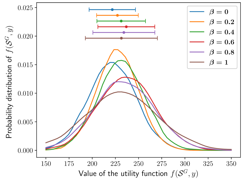
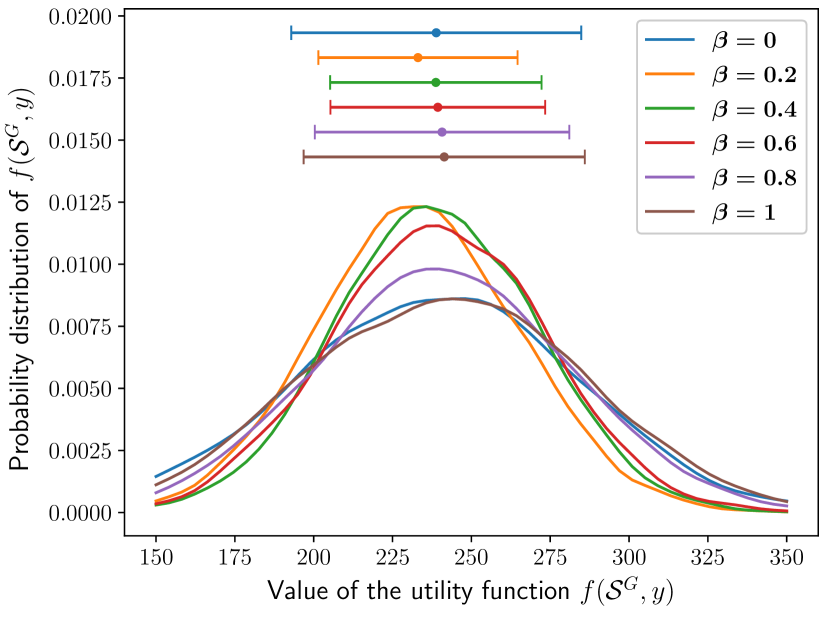
(a) $\alpha=0.1$

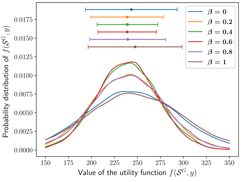
(b) $\alpha=0.4$

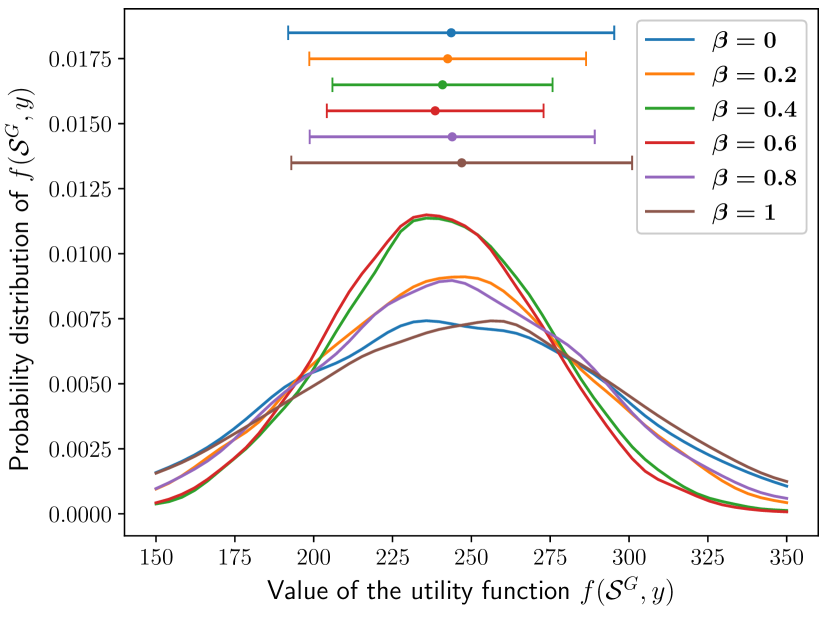
(c) $\alpha=0.7$

(d) $\alpha=1$

Figure 4: Probability density function of $f(\mathcal{S},y)$ at different values of $\beta$, keeping $\alpha$ fixed.

IV-A Algorithm

RAGA has three main stages:
(i) Initialization (lines 1 - 1) The decision set $\mathcal{S}$ (Hamiltonian cycle) is initialized as an empty set. A degree vector $D$ is set as $\mathbf{0}_{1\times|\mathcal{V}|}$, which contains vertices’ degrees in order. We use variables $\hat{H}_{\text{max}}=0$ and $\hat{H}_{\text{cur}}=0$ store the maximal and the current values of $\hat{H}(\mathcal{S},\tau)$ (line 1).
(ii) Search for valid tour for every $\tau$ (lines 1 - 1): For a specific value of $\tau$, we continue to add edges greedily until we have a complete tour or the edge set $\mathcal{E}$ is empty. For every edge $e\in\mathcal{E}\setminus\mathcal{S}$, we calculate the marginal gain of the auxiliary function, $\hat{H}(\mathcal{S}\cup\{e\})-\hat{H}(\mathcal{S})$ using the oracle function $\mathbb{O}$, and choose the edge $e^{*}$ which maximizes the marginal gain (line 1). We then check if the selected edge $e^{*}$ forms (or could form) a valid tour with the elements in $\mathcal{S}$ (i.e., if $\mathcal{S}\cup\{e^{*}\}\in\mathcal{I}$) (lines 1 - 1). Here, we first validate the degree constraint for each edge in $\mathcal{S}\cup\{e\}$, and then use the depth-first search (DFS) algorithm to iterate through the selected edges to check for subtours. If the new edge does not break the above constraints, we add the edge in $\mathcal{S}$ and update $D$ and $\hat{H}_{cur}$ (lines 1 - 1). Finally, we remove $e^{*}$ from $\mathcal{E}$ in line 1.
(iii) Selecting best tour set ($\mathcal{S}^{G},\tau^{G}$) (lines 1 - 1): For every tour we store the value of the auxiliary function $\hat{H}$ in $\hat{H}_{\text{cur}}$, and compare it to the best value $\hat{H}_{\text{max}}$. We store the pair $(\mathcal{S},\tau)$ whenever $\hat{H}_{\text{cur}}>\hat{H}_{\text{max}}$, and update $\hat{H}_{\text{max}}$.

Lines 1 - 1 show the condition of exiting the loop. As $H(\mathcal{S},\tau)$ is concave in $\tau$, and we start from a non-negative value (as seen in Fig. LABEL:fig:H_vs_tau), it is certain that if $H(\mathcal{S},\tau)$ becomes negative, it will continue to further decrease. This improves the runtime of RAGA.

Designing the oracle function $\mathbb{O}$: We use a sampling based oracle function to approximate $H(\mathcal{S},\tau)$ as $\hat{H}(\mathcal{S},\tau)$. The authors of [ohsaka2017portfolio] have proved that if the number of samples $n_{s}=O(\frac{\Gamma^{2}}{\epsilon^{2}}\log\frac{1}{\delta})$, $\delta,\epsilon\in(0,1)$, the approximation for the value of CVaR (or equivalently, the auxiliary function $\hat{H}(\mathcal{S},\tau)$) gives an error less than $\epsilon$ with a probability of at least $1-\delta$.

IV-B Performance Analysis

Theorem 1

Let $\mathcal{S}^{G}$ and $\tau^{G}$ be the tour and the searching scalar selected by RAGA and let $\mathcal{S}^{\star}$ and $\tau^{\star}$ be the tour and the searching scalar selected the optimal solution. Then,

$$H(\mathcal{S}^{G},\tau^{G})\geq\frac{1}{2+\mathit{k}}(H(\mathcal{S}^{\star},\tau^{\star})-\gamma)+\frac{1+\mathit{k}}{2+\mathit{k}}\Gamma(1-\frac{1}{\alpha})-\epsilon$$ (11)

with a probability of at least $1-\delta$, when the number of samples $n_{s}=O(\frac{\Gamma^{2}}{\epsilon^{2}}\log\frac{1}{\delta}),\;\delta,\epsilon\in(0,1)$. $k$ is the curvature of $H(\mathcal{S},\tau)$ with respect to $\mathcal{S}$.